Capital Deepening and Non-Balanced Economic Growth�

Daron AcemogluMIT

Veronica GuerrieriUniversity of Chicago

First Version: May 2004.This Version: March 2008.

Abstract

We present a model of non-balanced growth based on di¤erences in factor proportionsand capital deepening. Capital deepening increases the relative output of the more capital-intensive sector, but simultaneously induces a reallocation of capital and labor away fromthat sector. Using a two-sector general equilibrium model, we show that non-balancedgrowth is consistent with an asymptotic equilibrium with constant interest rate and capitalshare in national income. For plausible parameter values, the model generates dynamicsconsistent with US data, in particular, faster growth of employment and slower growth ofoutput in less capital-intensive sectors, and aggregate behavior consistent with the Kaldorfacts.

Keywords: capital deepening, multi-sector growth, non-balanced economic growth.JEL Classi�cation: O40, O41, O30.

�We thank John Laitner, Guido Lorenzoni, Iván Werning, three anonymous referees and especially the editorNancy Stokey for very helpful suggestions. We also thank seminar participants at Chicago, Federal ReserveBank of Richmond, IZA, MIT, NBER Economic Growth Group, 2005, Society of Economic Dynamics, Florence2004 and Vancouver 2006, Universitat of Pompeu Fabra for useful comments and Ariel Burstein for help withthe simulations. Acemoglu acknowledges �nancial support from the Russell Sage Foundation and the NSF.

1 Introduction

Most models of economic growth strive to be consistent with the �Kaldor facts�, i.e., the rela-

tive constancy of the growth rate, the capital-output ratio, the share of capital income in GDP

and the real interest rate (see Kaldor, 1963, and also Denison, 1974, Homer and Sylla, 1991,

Barro and Sala-i-Martin, 2004). Beneath this balanced picture, however, there are systematic

changes in the relative importance of various sectors (see Kuznets, 1957, 1973, Chenery, 1960,

Kongsamut, Rebelo and Xie, 2001). A recent literature develops models of economic growth

and development that are consistent with such structural changes, while still remaining ap-

proximately consistent with the Kaldor facts.1 This literature typically starts by positing

non-homothetic preferences consistent with Engel�s law and thus emphasizes the demand-side

reasons for non-balanced growth; the marginal rate of substitution between di¤erent goods

changes as an economy grows, directly leading to a pattern of uneven growth between sectors.

An alternative thesis, �rst proposed by Baumol (1967), emphasizes the potential non-balanced

nature of economic growth resulting from di¤erential productivity growth across sectors, but

has received less attention in the literature.2

In this paper, we present a two-sector model that highlights a natural supply-side reason for

non-balanced growth related to Baumol�s (1967) thesis. Di¤erences in factor proportions across

sectors (i.e., di¤erent shares of capital) combined with capital deepening lead to non-balanced

growth because an increase in capital-labor ratio raises output more in sectors with greater

capital intensity. We illustrate this economic mechanism using an economy with a constant

elasticity of substitution between two sectors and Cobb-Douglas production functions within

each sector. We show that the equilibrium (and the Pareto optimal) allocations feature non-

balanced growth at the sectoral level but are consistent with the Kaldor facts in the long run.

1See, for example, Matsuyama (1992), Echevarria (1997), Laitner (2000), Kongsamut, Rebelo and Xie (2001),Caselli and Coleman (2001), Gollin, Parente and Rogerson (2002). See also the interesting papers by Stokey(1988), Matsuyama (2002), Foellmi and Zweimuller (2002), and Buera and Kaboski (2006), which derive non-homothetiticites from the presence of a �hierarchy of needs� or �hierarchy of qualities�. Finally, Hall andJones (2006) point out that there are natural reasons for health care to be a superior good (because expectedlife expectancy multiplies utility) and show how this can account for the increase in health care spending.Matsuyama (2005) presents an excellent overview of this literature.

2Two exceptions are the recent independent papers by Ngai and Pissarides (2006) and Zuleta and Young(2006). Ngai and Pissarides (2006) construct a model of multi-sector economic growth inspired by Baumol. InNgai and Pissarides�s model, there are exogenous Total Factor Productivity di¤erences across sectors, but allsectors have identical Cobb-Douglas production functions. While both of these papers are potentially consistentwith the Kuznets and Kaldor facts, they do not contain the main contribution of our paper: non-balancedgrowth resulting from factor proportion di¤erences and capital deepening.

1

In the empirically relevant case where the elasticity of substitution between the two sectors is

less than one, one of the sectors (typically the more capital-intensive one) grows faster than

the rest of the economy, but because the relative prices move against this sector, its (price-

weighted) value grows at a slower rate than the rest of the economy. Moreover, we show that

capital and labor are continuously reallocated away from the more rapidly growing sector.3

Figure 1 shows that the distinctive qualitative implications of our model are consistent with

the broad patterns in the US data over the past 60 years. Motivated by our theory, this �gure

divides US industries into two groups according to their capital intensity and shows that there

is more rapid growth of �xed-price quantity indices (corresponding to real output) in the more

capital-intensive sectors, while (price-weighted) value of output and employment grow more

in the less capital-intensive sectors. The opposite movements of quantity and employment

(or value) between sectors with high and low capital intensities is a distinctive feature of our

approach (for the theoretically and empirically relevant case of the elasticity of substitution

less than one).4

Finally, we present a simple calibration of our model to investigate whether its quantita-

tive as well as its qualitative predictions are broadly consistent with US data. Even though

the model does not feature the demand-side factors that are undoubtedly important for non-

balanced growth, it generates relative growth rates of capital-intensive sectors that are consis-

tent with the US data over the past 60 years. For example, our calibration generates increases

in the relative output of the more capital-intensive industries that are consistent with the

changes in US data between 1948 and 2004 and accounts for one sixth to one third of the in-

crease in the relative employment of the less capital-intensive industries. Our calibration also

shows that convergence to the asymptotic (equilibrium) allocation is very slow, and consistent

with the Kaldor facts, along this transition path the share of capital in national income and

3As we will see below, in our economy the elasticity of substitution between products will be less than one ifand only if the (short-run) elasticity of substitution between labor and capital is less than one. The time-seriesand cross-industry evidence suggests that the short-run elasticity of substitution between labor and capitalis indeed less than one. See, for example, the surveys by Hamermesh (1993) and Nadiri (1970), which showthat the great majority of the estimates are less than one. Recent works by Krusell, Ohanian, Rios-Rull, andViolante (2000) and Antras (2001) also report estimates of the elasticity that are less than 1. Finally, estimatesimplied by the response of investment to the user cost of capital also typically imply an elasticity of substitutionbetween capital and labor signi�cantly less than 1 (see, e.g., Chirinko, 1993, Chirinko, Fazzari and Mayer, 1999,Mairesse, Hall and Mulkay, 1999).

4 It should be noted that the di¤erential evolutions of high and low capital intensity sectors shown in Figure 1is distinct from the major structural changes associated with changes in the share of agriculture, manufacturingand services. Our model does not attempt to account for these structural changes.

2

the interest rate are approximately constant.

The rest of the paper is organized as follows. Section 2 presents our model of non-balanced

growth, characterizes the full dynamic equilibrium of this economy, and shows how the model

generates non-balanced sectoral growth while remaining consistent with the Kaldor facts. Sec-

tion 3 undertakes a simple calibration of our benchmark economy to investigate whether the

dynamics generated by the model are consistent with the changes in the relative output and

employment of capital-intensive sectors and the Kaldor facts. Section 4 concludes. Appendix

A contains additional theoretical results, while Appendix B, which is available on the Web,

provides further details on the NIPA data and the sectoral classi�cations used in Figure 1 and

in Section 3, and additional evidence consistent with the patterns shown in Figure 1.

2 A Model of Non-Balanced Growth

In this section, we present the environment, which is a two-sector model with exogenous

technological change. The working paper version, Acemoglu and Guerrieri (2006), presents

results on non-balanced growth in a more general setting as well as an extension of the model

that incorporates endogenous technological change.

2.1 Demographics, Preferences and Technology

The economy admits a representative household with the standard preferencesZ 1

0exp (� (�� n) t) ~c(t)

1�� � 11� � dt; (1)

where ~c (t) is consumption per capita at time t, � is the rate of time preferences and � � 0

is the inverse of the intertemporal elasticity of substitution (or the coe¢ cient of relative risk

aversion). Labor is supplied inelastically and is equal to population L (t) at time t, which

grows at the exponential rate n 2 [0; �), so that

L (t) = exp (nt)L (0) : (2)

The unique �nal good is produced competitively by combining the output (intermediate

goods) of two sectors with an elasticity of substitution " 2 [0;1):

Y (t) = F [Y1 (t) ; Y2 (t)] (3)

=h Y1 (t)

"�1" + (1� )Y2 (t)

"�1"

i ""�1

;

3

where 2 (0; 1). Both sectors use labor, L, and capital, K. Capital depreciates at the rate

� � 0.

The aggregate resource constraint, which is equivalent to be the budget constraint of the

representative household, requires consumption and investment to be less than the output of

the �nal good,

_K (t) + �K (t) + C (t) � Y (t) ; (4)

where C (t) � ~c (t)L (t) is total consumption and investment consists of new capital, _K (t),

and replenishment of depreciated capital, �K (t).

The two goods Y1 and Y2 are produced competitively with production functions

Y1 (t) =M1 (t)L1 (t)�1 K1 (t)

1��1 and Y2 (t) =M2 (t)L2 (t)�2 K2 (t)

1��2 ; (5)

where K1; L1;K2 and L2 are the levels of capital and labor used in the two sectors.

If �1 = �2, the production function of the �nal good takes the standard Cobb-Douglas

form. Hence, we restrict attention to the case where �1 6= �2. Without loss of generality, we

assume that sector 1 is more labor intensive (or less capital intensive), that is,

� � �1 � �2 > 0: (A1)

Technological progress in both sectors is exogenous and takes the form

_M1 (t)

M1 (t)= m1 > 0 and

_M2 (t)

M2 (t)= m2 > 0: (6)

Capital and labor market clearing require that at each date

K1 (t) +K2 (t) � K (t) ; (7)

and

L1 (t) + L2 (t) � L (t) ; (8)

where K denotes the aggregate capital stock and L is total population. The restriction that

each of L1, L2, K1, and K2 has to be nonnegative is left implicit throughout.

2.2 The Competitive Equilibrium and the Social Planner�s Problem

Let us denote the rental price of capital and the wage rate by R and w and the interest rate

by r. Also let p1 and p2 be the prices of the Y1 and Y2 goods. We normalize the price of the

4

�nal good, P , to one at all points, so that

1 � P (t) =h "p1 (t)

1�" + (1� )" p2 (t)1�"i 11�"

: (9)

A competitive equilibrium is de�ned in the usual way as paths for factor and intermediate

goods prices [r (t) ; w (t) ; p1 (t) ; p2 (t)]t�0, employment and capital allocations

[L1 (t) ; L2 (t) ;K1 (t) ;K2 (t)]t�0 such that �rms maximize pro�ts, and markets clear, and con-

sumption and savings decisions [c (t) , _K (t)]t�0 which maximize the utility of the representative

household.

Since markets are complete and competitive, we can appeal to the Second Welfare Theo-

rem and characterize the competitive equilibrium by solving the social planner�s problem of

maximizing the utility of the representative household.5 This problem takes the form:

max[L1(t);L2(t);K1(t);K2(t);K(t);~c(t)]t�0

Z 1

0exp (� (�� n) t) ~c(t)

1�� � 11� � dt (SP)

subject to (2), (6), (7), (8), and the resource constraint

_K (t) + �K (t) + ~c (t)L (t) � Y (t) (10)

= FhM1 (t)L1 (t)

�1 K1 (t)1��1 ;M2 (t)L2 (t)

�2 K2 (t)1��2

i;

together with the initial conditions K (0) > 0, L (0) > 0, M1 (0) > 0 and M2 (0) > 0. The

objective function in this program is continuous and strictly concave, while the constraint

set forms a convex-valued continuous correspondence, thus the social planner�s problem has a

unique solution, and this solution corresponds to the unique competitive equilibrium.

Once this solution is characterized, the appropriate multipliers give the competitive prices.

For example, given the normalization in (9), which is equivalent to the multiplier on (10) being

normalized to one, the multipliers associated with (7) and (8) at time t give the rental rate,

R (t) � r (t) + �, and the wage rate, w (t), at time t. The prices of the intermediate goods are

then obtained as

p1 (t) =

�Y1 (t)

Y (t)

�� 1"

and p2 (t) = (1� )�Y2 (t)

Y (t)

�� 1"

: (11)

2.3 The Static Equilibrium

Inspection of (SP) shows that the maximization problem can be broken into two parts. First,

given the state variables, K (t), L (t),M1 (t) andM2 (t), the allocation of factors across sectors,5See Acemoglu and Guerrieri (2006) for an explicit characterization of the equilibrium.

5

L1 (t) ; L2 (t) ;K1 (t) and K2 (t), is chosen to maximize output Y (t) = F [Y1 (t) ; Y2 (t)] so as

to achieve the largest possible set of allocations that satisfy the constraint set. Second, given

this choice of factor allocations at each date, the time path of K (t) and ~c (t) can be chosen

to maximize the value of the objective function. These two parts correspond to the character-

ization of the static and dynamic optimal allocations, which are equivalent to the static and

dynamic equilibrium allocations. We �rst characterize the static equilibrium and the implied

competitive prices p1 (t), p2 (t), r (t) and w (t), and then turn to equilibrium dynamics.

Let us de�ne the maximized value of current output given capital stock K (t) at time t as

� (K (t) ; t) = maxL1(t);L2(t);K1(t);K2(t)

F [Y1 (t) ; Y2 (t)] (12)

subject to (5), (6), (7), (8);

and given K (t) > 0, L (t) > 0, M1 (t) > 0, M2 (t) > 0:

It is straightforward to see that this will involve the equalization of the marginal products of

capital and labor in the two sectors, which can be written as

�1

�Y (t)

Y1 (t)

� 1" Y1 (t)

L1 (t)= (1� )�2

�Y (t)

Y2 (t)

� 1" Y2 (t)

L2 (t); (13)

and

(1� �1)�Y (t)

Y1 (t)

� 1" Y1 (t)

K1 (t)= (1� ) (1� �2)

�Y (t)

Y2 (t)

� 1" Y2 (t)

K2 (t): (14)

Since the key static decision involves the allocation of labor and capital between the two sectors,

we de�ne the shares of capital and labor allocated to the labor-intensive sector (sector 1) as

� (t) � K1 (t)

K (t)and � (t) � L1 (t)

L (t):

Clearly, we also have 1 � � (t) � K2 (t) =K (t) and 1 � � (t) � L2 (t) =L (t). Combining (13)

and (14), we obtain

� (t) =

"1 +

�1� �21� �1

��1�

��Y1 (t)

Y2 (t)

� 1�""

#�1(15)

and

� (t) =

�1 +

�1� �11� �2

���2�1

��1� � (t)� (t)

���1: (16)

Equation (16) shows that, at each time t, the share of labor in sector 1, � (t), is (strictly)

increasing in � (t). We next determine how these two shares change with capital accumulation

and technological change.

6

Proposition 1 In the competitive equilibrium,

d ln� (t)

d lnK (t)= � d ln� (t)

d lnL (t)=

(1� ")� (1� � (t))1 + (1� ")� (� (t)� � (t)) > 0, �(1� ") > 0; and (17)

d ln� (t)

d lnM2 (t)= � d ln� (t)

d lnM1 (t)=

(1� ") (1� � (t))1 + (1� ")� (� (t)� � (t)) > 0, " < 1: (18)

Proof. To derive these expressions, rewrite (15) as

� (�; L;K;M1;M2) � ��"1 +

�1� �21� �1

��1�

��Y1Y2

� 1�""

#�1= 0;

where, from (5),

Y1Y2= ��1 (1� �)��2 �1��1 (1� �)�(1��2)

�L

K

�� M1

M2;

with � given as in (16). Applying the Implicit Function Theorem to � (�; L;K;M1;M2) and

using the expression for Y1=Y2 given here, we obtain (17) and (18).

Equation (17) states that the fraction of capital allocated to the labor-intensive sector

increases with the stock of capital if " < 1 and it increases if " > 1. To obtain the intuition for

this comparative static, which is useful for understanding many of the results that will follow,

note that if K increased and � remained constant, then the capital-intensive sector, sector 2,

would grow by more than sector 1� because an equi-proportionate increase in capital raises the

output of the more capital-intensive sector by more. The prices of intermediate goods given in

(11) then imply that when " < 1, the relative price of the capital-intensive sector will fall more

than proportionately, inducing a greater fraction of capital to be allocated to the less capital-

intensive sector 1. The intuition for the converse result when " > 1 is straightforward. An

important implication of this proposition is that as long as " 6= 1 and there is capital deepening

(i.e., as long as K=L is increasing over time), growth will be non-balanced and capital will

be allocated unequally between the two sectors. This is the basis of non-balanced growth in

our model.6 The rest of our analysis will show that non-balanced growth in this model is

consistent with the Kaldor facts asymptotically and can approximate the Kaldor facts even

along transitional dynamics.

Equation (18) also implies that when the elasticity of substitution, ", is less than one, an

improvement in the technology of a sector causes the share of capital allocated to that sector6As a corollary, note that with " = 1, output levels in the two sectors could grow at di¤erent rates, but there

would be no reallocation of capital and labor between the two sectors, and � and � would remain constant.

7

to fall. The intuition is again the same: when " < 1, increased production in a sector causes

a more than proportional decline in its relative price, inducing a reallocation of capital away

from it towards the other sector (again the converse results and intuition apply when " > 1).

In view of equation (16), the results in Proposition 1 also apply to �. In particular, we

have that d ln� (t) =d lnK (t) = �d ln� (t) =d lnL (t) > 0 if and only if �(1� ") > 0.

Next, since equilibrium factor prices, R and w, correspond to the multipliers on the con-

straints (7) and (8), we also obtain

w (t) = �1

�Y (t)

Y1 (t)

� 1" Y1 (t)

L1 (t); (19)

and

R (t) = �K (K (t) ; t) = (1� �1)�Y (t)

Y1 (t)

� 1" Y1 (t)

K1 (t); (20)

where �K (K (t) ; t) is the derivative of the maximized output function, � (K (t) ; t), with re-

spect to capital. Equilibrium factor prices take the familiar forms and are equal to the (values

of) marginal products from the derived production function in (10). To obtain an intuition for

the economic forces, we next analyze how changes in the state variables, L, K, M1 and M2,

impact on these factor prices. Combining (19) and (20), relative factor prices are obtained as

w (t)

R (t)=

�11� �1

�� (t)K (t)

� (t)L (t)

�; (21)

and the capital share in aggregate income is

�K (t) �R (t)K (t)

Y (t)= (1� �1)

�Y (t)

Y1 (t)

� 1�""

� (t)�1 : (22)

Proposition 2 In the competitive equilibrium,

d ln (w (t) =R (t))

d lnK (t)= �d ln (w (t) =R (t))

d lnL (t)=

1

1 + (1� ")� (� (t)� � (t)) > 0;

d ln (w (t) =R (t))

d lnM2 (t)= �d ln (w (t) =R (t))

d lnM1 (t)

= � (1� ") (� (t)� � (t))1 + (1� ")� (� (t)� � (t)) < 0, �(1� ") > 0;

d ln�K (t)

d lnK (t)= � (1� ")�2 (1� � (t))� (t)

[1� �1 +�� (t)] [1 + (1� ")� (� (t)� � (t))]< 0, " < 1; and (23)

8

d ln�K (t)

d lnM2 (t)= �d ln�K (t)

d lnM1 (t)(24)

=�(1� ") (1� � (t))� (t)

[1� �1 +�� (t)] [1 + (1� ")� (� (t)� � (t))]< 0

, �(1� ") > 0:

Proof. The �rst two expressions follow from di¤erentiating equation (21) and Proposition

1. To prove (23) and (24), note that from (3) and (15), we have�Y1Y

� "�1"

= �1�1 +

�1� �11� �2

��1� ��

���1:

Then, (23) and (24) follow by di¤erentiating �K as given in (22) with respect to L, K, M1 and

M2, and using the results in Proposition 1.

The most important result in this proposition is (23), which links the impact of the capital

stock on the capital share in national income to the elasticity of substitution between the

two sectors, ". Since a negative relationship between the share of capital in national income

and the capital stock is equivalent to an elasticity of substitution between aggregate labor

and capital that is less than one, this result also implies that, as claimed in footnote 3, the

elasticity of substitution between capital and labor is less than one if and only if " is less

than one. Intuitively, an increase in the capital stock of the economy causes the output of the

more capital-intensive sector, sector 2, to increase relative to the output in the less capital-

intensive sector (despite the fact that the share of capital allocated to the less-capital intensive

sector increases as shown in equation (17)). This then increases the production of the more

capital-intensive sector, and when " < 1, it reduces the relative price of capital more than

proportionately; consequently, the share of capital in national income declines. The converse

result applies when " > 1.

Moreover, when " < 1, (24) implies that an increase in M1 is �capital biased� and an

increase in M2 is �labor biased�. The intuition for why an increase in the productivity of the

sector that is intensive in capital is biased toward labor (and vice versa) is once again similar:

when the elasticity of substitution between the two sectors, ", is less than one, an increase in

the output of a sector (this time driven by a change in technology) decreases its price more than

proportionately, thus reducing the relative compensation of the factor used more intensively in

that sector (see Acemoglu, 2002). When " > 1, we have the converse pattern, and an increase

in M1 is �labor biased,�while an increase in M2 is �capital biased�.

9

2.4 Equilibrium Dynamics

We now characterize the dynamic competitive equilibrium allocations. We again use the social

planner�s problem (SP) introduced above. The previous subsection characterized the static

optimal (equilibrium) allocation of resources and the resulting maximized value of output

� (K (t) ; t) for given values of K (t), L (t), M1 (t), and M2 (t). Given � (K (t) ; t), problem

(SP) can be written as

max[K(t);~c(t)]t�0

Z 1

0exp (� (�� n) t) ~c (t)

1�� � 11� � dt (SP0)

subject to

_K (t) = � (K (t) ; t)� �K (t)� exp (nt)L (0) ~c (t) ; (25)

and the initial condition K (0) > 0. The constraint (25) is written as an equality since it

cannot hold as a strict inequality in an optimal allocation (otherwise, consumption would be

raised, yielding a higher objective value). The other initial conditions of the original problem

(SP) are incorporated into the maximized value of output � (K (t) ; t) in constraint (25). This

maximization problem is simpler than (SP), though it is still not equivalent to the standard

problems encountered in growth models because constraint (25) is not an autonomous di¤er-

ential equation. To further simplify the characterization of equilibrium dynamics, we will work

with transformed variables. For this purpose, we �rst assume:

either (i) m1=�1 < m2=�2 and " < 1; or (ii) m1=�1 > m2=�2 and " > 1; (A2)

which ensures that the asymptotically dominant sector will be the labor-intensive sector, sector

1. The asymptotically dominant sector is the sector that determines the long-run growth rate

of the economy. Observe that this condition compares not the exogenous rates of technological

progress, m1 and m2, but m1=�1 and m2=�2, which we refer to as the augmented rates of

technological progress. This is because the two sectors di¤er in terms of their capital intensities,

and technological change will be augmented by the di¤erential rates of capital accumulation

in the two sectors. For example, with equal rates of Hicks-neutral technological progress in

the two sectors, the adjustment of the capital stock to technological change implies that the

labor-intensive sector 1 will have a lower augmented rate of technological progress than sector

2.

Notice that when " < 1, the sector with the lower rate of augmented technological progress

will be the asymptotically dominant sector. This is because, when " < 1, the output of the two

10

sectors are highly complementary and the slower growing sector will determine the asymptotic

growth rate of the economy. When " > 1, the converse happens and the more rapidly grow-

ing sector determines the asymptotic growth rate of the economy and is the asymptotically

dominant sector. In this light, Assumption (A2) implies that sector 1 is the asymptotically

dominant sector. Appendix A shows that parallel results apply when the converse of (A2)

holds and sector 2 is asymptotically dominant. The empirically relevant case is part (i) of

Assumption (A2); as already argued, " < 1 provides a good approximation to the data, and

�1 > �2 from (A1). Therefore, as long as m1 and m2 are close to each other, the economy will

be in case (i) of (A2).

Let us next introduce the following normalized variables,

c (t) � ~c (t)

M1 (t)1=�1

and � (t) � K (t)

L (t)M1 (t)1=�1

; (26)

which represent consumption and capital per capita normalized by the augmented technology

of the asymptotically dominant sector, which, in view of Assumption (A2), is sector 1 (and

thus the corresponding augmented technology is M1 (t)1=�1). Next proposition shows that

the solution to (SP)� and thus the dynamic equilibrium� can be expressed in terms of three

autonomous di¤erential equations in c, � and �.

Proposition 3 Suppose that (A1) and (A2) hold. Then, a competitive equilibrium satis�es

the following three di¤erential equations

_c (t)

c (t)=

1

�

h(1� �1) � (t)1=" � (t)�1 � (t)��1 � (t)��1 � � � �

i� m1

�1; (27)

_� (t)

� (t)= � (t)�1 � (t)1��1 � (t)��1 � (t)� � (t)�1 c (t)� � � n� m1

�1;

_� (t)

� (t)=

(1� � (t))h� _�(t)�(t) +m2 � �2

�1m1

i(1� ")�1 +�(� (t)� � (t))

;

where

� (t) � "

"�1

�1 +

�1� �11� �2

��1� � (t)� (t)

�� ""�1

; (28)

with initial conditions � (0) and � (0), and also satis�es the transversality condition

limt!1

exp

����� (1� �)m1

�1� n

�t

�� (t) = 0: (29)

Moreover, any allocation that satis�es (27)-(29) is a competitive equilibrium.

11

Proof. See Appendix A.

The �rst equation in (27) is the standard Euler equation, written in terms of the normalized

variables. The �rst term in square brackets, (1� �1) � (t)1=" � (t)�1 � (t)��1 � (t)��1 , is the

marginal product of capital. The second equation in (27) is the law of motion of the normalized

capital stock, � (t). The third equation, in turn, speci�es the evolution of the share of capital

between the two sectors. We also impose the following parameter condition, which ensures

that the transversality condition (29) holds:

�� n � (1� �) m1

�1: (A3)

Our next task is to use Proposition 3 to provide a tighter characterization of the dynamic

equilibrium allocation. For this purpose, let us �rst de�ne a Constant Growth Path (CGP)

as a dynamic competitive equilibrium that features constant aggregate consumption growth.7

The next theorem will show that there exists a unique CGP that is a solution to the social

planner�s problem (SP) and will provide closed-form solutions for the growth rates of di¤erent

aggregates in this equilibrium. The notable feature of the CGP will be that despite the constant

growth rate of aggregate consumption, growth will be non-balanced because output, capital

and employment in the two sectors will grow at di¤erent rates. Let us de�ne:

_Ls (t)

Ls (t)� ns (t) ;

_Ks (t)

Ks (t)� zs (t) ;

_Ys (t)

Ys (t)� gs (t) for s = 1; 2, and

_K (t)

K (t)� z (t) ;

_Y (t)

Y (t)� g (t) ;

so that ns and zs denote the growth rates of labor and capital stock, ms denotes the growth

rate of technology, and gs denotes the growth rate of output in sector s. Moreover, when-

ever they exist, we denote the corresponding asymptotic growth rates by asterisks, so that

n�s = limt!1 ns (t), z�s = limt!1 zs (t), and g�s = limt!1 gs (t). Similarly, let us denote the

asymptotic capital and labor allocation decisions by asterisks, that is,

�� = limt!1

� (t) and �� = limt!1

� (t) :

Then we have the following characterization of the unique CGP.

Theorem 1 Suppose that (A1)-(A3) hold. Then, there exists a unique CGP where consump-

tion per capita grows at the rate g�c = m1=�1, and �� = 1,

�� =

"(�m1=�1 + �+ �)

"

"�1 (1� �1)

#� 1�1

; (30)

7Kongsamut, Rebelo and Xie (2001) refer to this as a �Generalized Balanced Growth Path�.

12

and

c� = "

"�1 (��)1��1 � ���� + n+

m1

�1

�: (31)

Moreover, the growth rates of output, capital and employment in the two sectors are

g� = g�1 = z� = z�1 = n+

m1

�1; (32)

z�2 = g� � (1� ")!; (33)

g�2 = g� + "!; (34)

n�1 = n and n�2 = n� (1� ")!; (35)

where

! � m2 ��2�1m1:

Proof. From Proposition 3, a competitive equilibrium satis�es (27)-(29). A CGP requires

that limt!1 _c (t) =c (t) is constant, thus from the �rst equation of (27),

� (t)1=" � (t)�1 � (t)��1 � (t)��1 must be constant as t!1. Consequently, as t!1,

1

"

_� (t)

� (t)+ �1

_� (t)

� (t)� �1

_� (t)

� (t)� �1

_� (t)

� (t)= 0: (36)

Di¤erentiating (16) and (28) with respect to time and using the third equation of the system

(27), we obtain expressions for _� (t) =� (t), _� (t) =� (t), and _� (t) =� (t) in terms of _� (t) =� (t).

Substituting these into (36) and rearranging, we can express (36) as an autonomous �rst-order

di¤erential equation in � (t) as

_� (t)

� (t)= G (� (t))�1�2 (1� ")

�m2

�2� m1

�1

�; (37)

where

G (� (t)) =[�� (t) + (1� �1)] (1� � (t))

�� (t) + �2 (1� �1):

Clearly, G (0) = 1=�2, G (1) = 0 and G0 (�) < 0 for any �. These observations together with

Assumption (A2) imply that (37) has a unique solution with � (t)! �� = 1. Next, _� (t) =� (t) =

0 combined with (16) and (28) implies that _� (t) =� (t) = _� (t) =� (t) = 0. Moreover, given

� (t) ! �� = 1, (16) implies � (t) ! �� = 1 and (28) implies � (t) ! �� = "=("�1). Equation

(36) then implies that limt!1 � (t) = �� 2 (0;1) must also exist, thus _� (t) =� (t) ! 0. Now

setting the �rst two equations in (27) equal to zero and using the fact that �� = �� = 1 and

13

�� = "=("�1), we obtain (30) and (31). By construction, there are no other allocations with

constant _c (t) =c (t).

To derive equations (32)-(35), combine (26) with the result that _� (t) =� (t) ! 0, which

implies z� = n+m1=�1. Moreover, �� = �� = 1 together with the market clearing conditions

(7) and (8)� holding as equalities� give z�1 = z� and n�1 = n. Finally, di¤erentiating (3), (5),

(13) and (14), and using the preceding results, we obtain (32)-(35) as unique solutions.

To complete the proof that this allocation is the unique CGP we need to establish that

it satis�es the transversality condition (29). This follows immediately from the fact that

limt!1 � (t) = �� exists and is �nite combined with Assumption (A3), which implies that

limt!1 exp (� (�� (1� �)m1=�1 � n) t) = 0.

There are a number of important implications of this theorem. First, growth is non-

balanced, in the sense that the two sectors grow at di¤erent asymptotic rates (i.e., at di¤erent

rates even as t ! 1). The intuition for this result is more general than the speci�c para-

metrization of the model and is driven by the juxtaposition of factor proportion di¤erences

between sectors and capital deepening. In particular, suppose that there is capital deepening

(which here is due to technological progress). Now, if both capital and labor were allocated to

the two sectors in constant proportions, the more capital-intensive sector, sector 2, would grow

faster than sector 1. The faster growth in sector 2 would reduce the price of sector 2, leading to

a reallocation of capital and labor towards sector 1. However, this reallocation cannot entirely

o¤set the greater increase in the output of sector 2, since, if it did, the change in prices that

stimulated the reallocation would not take place. Therefore, growth must be non-balanced. In

particular, if " < 1, capital and labor will be reallocated away from the more rapidly growing

sector towards the more slowly growing sector. In this case, the more slowly growing sector,

sector 1, becomes the asymptotically dominant sector and determines the growth rate of ag-

gregate output as shown in equation (32). Note that sector 1 is the one growing more slowly

because Assumption (A2), together with " < 1, implies m1=�1 < m2=�2. Hence, Y1=Y2 ! 0.

Appendix A shows that similar results apply when the converse of (A2) holds.

Second, the theorem shows that in the CGP the shares of capital and labor allocated to

sector 1 tend to one (i.e., �� = �� = 1). Nevertheless, at all points in time both sectors produce

positive amounts and both sectors grow at rates greater than the rate of population growth (so

this limit point is never reached). Moreover, in the more interesting case where " < 1, equation

(34) implies g�2 > g� = g�1, so that the sector that is shedding capital and labor (sector 2) is

14

growing faster than the rest of the economy, even asymptotically. Therefore, the rate at which

capital and labor are allocated away from this sector is determined in equilibrium to be exactly

such that this sector still grows faster than the rest of the economy. This is the sense in which

non-balanced growth is not a trivial outcome in this economy (with one of the sectors shutting

down), but results from the positive and di¤erential growth of the two sectors.

Finally, it can be veri�ed that the share of capital in national income and the interest rate

are constant in the CGP. For example, under (A2), we have ��K = 1 � �1. This implies that

the asymptotic capital share in national income will re�ect the capital share of the dominant

sector. Also, again under (A2), the asymptotic interest rate is

r� = (1� �1) "

"�1 (��)��1 � �:

These results are the basis of the claim in the Introduction that this economy features both non-

balanced growth at the sectoral level and aggregate growth consistent with the Kaldor facts.

In particular, the CGP matches both the Kaldor facts and generates unequal growth between

the two sectors. However, at the CGP one of the sectors has already become (vanishingly)

small relative to the other. Therefore, this theorem does not answer the question of whether we

can have a situation in which both sectors have non-trivial employment levels and the capital

share in national income and the interest rate are approximately constant. This question is

investigated quantitatively in the next section. Before doing so, we establish the stability of

the CGP.

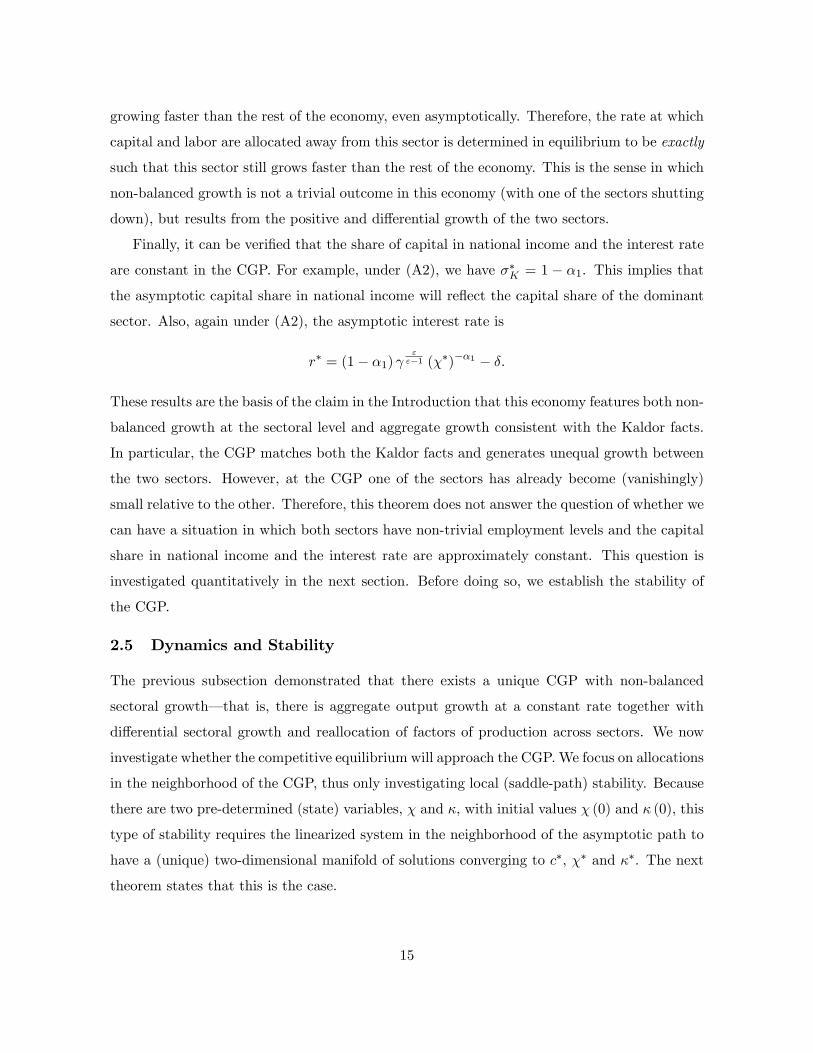
2.5 Dynamics and Stability

The previous subsection demonstrated that there exists a unique CGP with non-balanced

sectoral growth� that is, there is aggregate output growth at a constant rate together with

di¤erential sectoral growth and reallocation of factors of production across sectors. We now

investigate whether the competitive equilibrium will approach the CGP. We focus on allocations

in the neighborhood of the CGP, thus only investigating local (saddle-path) stability. Because

there are two pre-determined (state) variables, � and �, with initial values � (0) and � (0), this

type of stability requires the linearized system in the neighborhood of the asymptotic path to

have a (unique) two-dimensional manifold of solutions converging to c�, �� and ��. The next

theorem states that this is the case.

15

Theorem 2 Suppose that (A1)-(A3) hold. Then, the competitive equilibrium, given by (27),

is locally (saddle-path) stable, in the sense that in the neighborhood of c�, �� and ��; there is

a unique two-dimensional manifold of solutions that converge to c�, �� and ��.

Proof. Let us rewrite the system (27) in a more compact form as

_x = f (x) ; (38)

where x � ( c � � )0 is the transpose of the row vector ( c � � ). To investigate the

dynamics of the system (38) in the neighborhood of the steady state, consider the linear

system

_z = J (x�) z;

where z � x�x� and x� is such that f (x�) = 0, where J (x�) is the Jacobian of f (x) evaluated

at x�. Di¤erentiation and some algebra enable us to write this Jacobian matrix as

J (x�) =

0@ 0 ac� ac��1 a�� a��0 0 a��

1A :Hence, the determinant of the Jacobian is det J (x�) = �a��ac�, where

a�� = � (1� ")�m2 �

�2�1m1

�;

ac� = � "

"�1 (��)��1�1 �1 (1� �1)

�:

The above expressions show that both a�� and ac� are (strictly) negative, since, in view of

(A2), " 7 1 , m2=�2 ? m1=�1. This establishes that det J (x�) > 0, so the steady state

corresponding to the CGP is hyperbolic (that is, all eigenvalues of the Jacobian evaluated at

x� have nonzero real parts) and thus the dynamics of the linearized system represent the local

dynamics of the nonlinear system (see, e.g., Acemoglu, 2008, Theorem B.7). Moreover, either

all the eigenvalues are positive or two of them are negative and one is positive. To determine

which one of these two possibilities is the case, we look at the characteristic equation given

by det (J (x�)� vI) = 0, where v denotes the vector of the eigenvalues. This equation can be

expressed as the following cubic in v, with roots corresponding to the eigenvalues:

(a�� � v) [v (a�� � v) + a�cac�] = 0:

16

This expression implies that one of the eigenvalue is equal to a�� and thus negative, so there

must be two negative eigenvalues. This establishes the existence of a unique two-dimensional

manifold of solutions in the neighborhood of this CGP, converging to it.

This theorem establishes that the CGP is locally (saddle-path) stable, and when the initial

values of capital, labor and technology are not too far from the constant growth path, the

competitive equilibrium converges to this CGP, with non-balanced growth at the sectoral level

and constant capital share and interest rate at the aggregate.

3 A Simple Calibration

We now undertake an illustrative calibration to investigate whether the equilibrium dynamics

generated by our model economy are broadly consistent with the patterns in the US data. For

this exercise, we use data from the National Income and Product Accounts (NIPA) between

1948 and 2005. Industries are classi�ed according to North American Industrial Classi�cation

System (NAICS) at the 22-industry level of detail.8 We use industry-level data for current-price

value added (which we refer to as value), chain-type �xed-price quantity indices for value added

(which we refer to as quantity), total number of employees,9 total employee compensation, and

�xed assets. To map our model to data, we classify industries into low and high capital intensity

�sectors�, each comprising approximately 50% of total employment. Table 1 below shows the

average capital share for each industry and the sector classi�cation.10

Figure 1 in the introduction depicts the evolution of relative quantity, value, and employ-

ment in these sectors and shows the more rapid growth of quantity in the capital-intensive

sectors and the more rapid growth of value and employment in the less capital-intensive sec-

tors.11

For our calibration, we take the initial year, t = 0, to correspond to the �rst year for

8Throughout, we exclude the Government and Private household sectors and Agriculture, forestry, �shing,and hunting and Real estate and rental.

9 In particular, we use full-time and part-time employees, since this is the only measure for which we haveconsistent NAICS data going back to 1948. The alternative classi�cation system, SIC, does not enable us toextend data to 2005 and also reports the quantity indices for value added only back to 1977.10NAICS data on compensation of employees are only available between 1987 and 2005 (all the other variables

are available between 1948 and 2005). We therefore compute the capital share of each industry as the averagecapital share between 1987 and 2005. The average capital shares in the two sectors are relatively stable overtime. In particular, the average capital share of sector 1 is 0:288 in 1987 and 0:290 in 2005, while the averagecapital share of sector 2 is 0:466 in 1987 and 0:499 in 2005.11Appendix B provides more details on data sources and constructions. It also shows that the general patterns

in the US data, in particular those plotted in Figure 1, are robust to changing in the cuto¤ between high andlow capital-intensity industries.

17

which we have NIPA data for our sectors, 1948. In our model, L (t) corresponds to total

employment at time t, K (t) to �xed assets, Yj (t) to the quantity of output in sector j, and

Y Nj (t) � pj (t)Yj (t) to the value of output in sector j.

Our model economy is fully characterized by ten parameters �, �, �, , ", �1, �2, n, m1 and

m2, and �ve initial values, L (0), K (0), M1 (0), M2 (0) and � (0). We choose these parameters

and initial values as follows. First, we adopt the standard parameter values for the annual

discount rate, � = 0:02, the annual depreciation rate, � = 0:05, and the annual (asymptotic)

interest rate, r� = 0:08.12 We take the annual population growth rate n = 0:018 from the

NIPA data on employment growth for 1948-2005 and choose the asymptotic growth rate to

ensure that our calibration matches total output growth between 1948 and 2005 in the NIPA,

which is 3:4%. This implies an asymptotic growth rate of g� = 0:033. The initial values

L (0) = 40; 3360; 000 and K (0) = 244; 900 (in millions of dollars) are also directly from the

NIPA data for 1948. Next, our classi�cation of industries leads to two �aggregate sectors�with

average shares of labor in value added of 0:72 and 0:52. In terms of our model this implies

�1 = 0:72 and �2 = 0:52.

An important parameter for our calibration is the elasticity of substitution between the

two sectors. Although we do not have independent information on this variable, our model

suggests a way of evaluating this elasticity. In particular, equation (11) implies the following

relationship between value and quantity ratios in the two sectors:

log

�Y N1 (t)

Y N2 (t)

�= log

�

1�

�+"� 1"

log

�Y1 (t)

Y2 (t)

�. (39)

We can therefore estimate ("� 1) =" by regressing the log of the ratio of the nominal value

added between the two sectors on the log of the ratio of the real value added. Since our focus is

on medium-run frequencies (rather than business cycle �uctuations), we use the Hodrick and

Prescott �lter to smooth both the dependent and the independent variables (with smoothing

weight 1600) and use the smoothed variables to estimate (39). This simple regression yields an

estimate of " ' 0:76 (and a two standard error con�dence interval of [0:73; 0:79]). We therefore

choose " = 0:76 for our benchmark calibration. We also choose the parameter to ensure that

equation (39) holds at t = 0.

Throughout, motivated by our estimate of " reported in the previous paragraph, the existing

evidence discussed in footnote 3, and the pattern shown in Figure 1 indicating that employment12These numbers are the same as those used by Barro and Sala-i-Martin (2004) in their calibration of the

baseline neoclassical model.

18

and value grow more in the less capital-intensive sector, we focus on the case in which " < 1 and

m1=�1 < m2=�2 (case (i) of Assumption (A2)). In particular, for our benchmark calibration

we set m1 = m2 (even though, as we will see below, higher values of m2 improve the �t of

the model to US data). Since in this case sector 1 is the asymptotically dominant sector, the

asymptotic growth rate of output is g� = n + m1=�1. The above-mentioned values of g�, n

and �1 imply m1 = m2 = 0:0108. The growth rate of output also pins down the intertemporal

elasticity of substitution. In particular, the Euler equation (27) together with (26) yields

g� = (r� � �) =�+n, which implies � = 4 and results in a reasonable elasticity of intertemporal

substitution of 0:25.

This leaves us with the initial values for �, M1 and M2. First, notice that equation (15) at

time 0 can be rewritten as:

� (0) =

�1 +

�1� �21� �1

�Y N2 (0)

Y N1 (0)

��1: (40)

This equation together with the 1948 levels of values in the two sectors from the NIPA data,

Y N1 (0) and Y N2 (0), gives � (0) = 0:32. Equation (16) then gives the initial value of relative

employment as � (0) = 0:52.13 It is also worth noting that in addition to the parameters and the

initial values necessary for our calibration, the numbers we are using also pin down the initial

interest rate and the capital share in national income as r (0) = 0:095 and �K (0) = 0:39.14

Moreover, since sector 1 is the asymptotically dominant sector, the asymptotic capital share in

national income and the interest rate are determined as ��K = 1��1 = 0:28 and r� = 0:08. This

implies that, by construction, both the interest rate and the capital share must decline at some

point along the transition path. A key question concerns the speed of these declines. If this

happened at the same frequency as the change in the composition of employment and capital

across the two sectors, then the model would not generate a pattern that is simultaneously

consistent with non-balanced sectoral growth and the aggregate Kaldor facts. We will see that

this is not the case and that the model�s implications are broadly consistent with both sets of

facts.13We can also compute the empirical counterparts of � (0) and � (0) from the NIPA data using employment

and capital in the two sector aggregates. These give the values of 0:49 and 0:50, which are similar, thoughclearly not identical, to the implied values we use. The fact that the theoretically-implied values of � (0) and� (0) di¤er from their empirical counterparts is not surprising, since we are assuming that the US economy canbe represented by two sectors with Cobb-Douglas production functions and with their output being combinedwith a constant elasticity of substitution. Naturally, this is at best an approximation, and in the data, sectoralfactor intensities are not constant over time.14This is because the capital share and interest rate are functions of � only (just combine (20) and (22) with

(3) and (15)).

19

Finally, given � (0) = 0:32 and � (0) = 0:52, the NIPA data imply values for L1 (0), L2 (0),

K1 (0) and K2 (0), and we also have the values for Y1 (0) and Y2 (0) directly from the NIPA. We

then obtain the remaining initial values, M1 (0) andM2 (0), from equation (5). This completes

the determination of all the parameters and initial conditions of our model. We then compute

the time path of all the variables in our model using two di¤erent numerical procedures (both

giving equivalent results).15

Figure 2 shows the results of our benchmark calibration with the parameter values described

above. In particular, in this benchmark we have " = 0:76 and m1 = m2 = 0:0108. The four

panels depict relative employment in sector 1 (�), relative capital in sector 1 (�), the interest

rate (r) and the capital share in national income (�K) for the �rst 150 years (in terms of data,

corresponding to 1948 to 2098).

A number of features are worth noting. First, for the �rst 150 years, there is signi�cant

reallocation of capital and labor away from the more capital-intensive sector towards the less

capital-intensive sector, sector 1, and the economy is far from the asymptotic equilibrium

with � = � = 1. In fact, the economy takes a very long time, over 5000 years, to reach the

asymptotic equilibrium. This illustrates that our model economy generates interesting and

relatively slow dynamics, with a signi�cant amount of structural change. Second, while there

is non-balanced growth at the sectoral level, the interest rate and the capital share remain

approximately constant. The interest rate shows an early decline from about 9.5% to 9%,

which largely re�ects the initial consumption dynamics. It then remains around 9%. The

capital share shows a very slight decline over the 150 years. This relative constancy of the

interest-rate and the capital share is particularly interesting, since as noted above, we know

that both variables have to decline at some point to achieve their asymptotic values of r� = 0:08

and ��K = 0:28. Nevertheless, our model calibration implies more rapid structural change than

15 In particular, we �rst return to the two-dimensional non-autonomous system of equations in c and � (ratherthan the three-dimensional representation used for theoretical analysis in Proposition 3). This two dimensionalsystem has one state and one control variable. Following Judd (1998, Chapter 10), we discretize these di¤erentialequations using the Euler method to obtain a system of �rst-order di¤erence equations in c (t) and � (t). Thissystem can in turn be transformed into a second-order non-autonomous system in � (t), which is easier towork with. We then compute the numerical solution to this second-order di¤erence equation using either ashooting algorithm or by minimizing the squared residuals. Our main numerical method is to use a basicshooting algorithm starting with initial value of � (0), and then guess and adjust the value for � (1) to ensureconvergence to the asymptotic CGP. The second numerical procedure is to choose a polynomial form for thenormalized capital stock as � (t) = � (t;�), where � represents the parameters of the polynomial. We estimate� by minimizing the squared residuals of the di¤erence equations using nonlinear least squares (see, e.g., Judd,1998, Chapter 4) and then compute c (t) and � (t). The two procedures give almost identical results, andthroughout we report the results from the shooting algorithm.

20

the speed of these aggregate changes, and thus over the horizon of about 150 years, there is

little change in the interest rate and the capital share, while there is signi�cant reallocation of

labor and capital across sectors.

These patterns are further illustrated in Table 2, which shows the US data and the numbers

implied by our benchmark calibration between 1948 and 2005 for the relative quantity and

relative employment of the high versus low capital intensity sectors as well as the aggregate

capital share in national income (in terms of the model, t = 0 is taken to correspond to

1948, thus t = 57 gives the values for 2005). The �rst two columns of this table con�rm the

patterns shown in Figure 1 in the Introduction� quantity grows faster in high capital intensity

industries, while employment grows faster in low capital intensity industries. The next two

columns show that the benchmark calibration is broadly consistent with this pattern. In

particular, while in the data, Y2=Y1 increases by about 19% between 1948 and 2004, the model

leads to an increase of about 17%. In the data, L2=L1 declines by about 33%.16 In the model,

the implied decline is in the same direction, but considerably smaller, about 5%.17 However,

the evolutions of the capital share in the data and in the model are very similar. In the data,

the capital share declines from 0:398 to 0:396, whereas in the model it declines from 0:392 to

0:389.18

Table 3 and Table 4 show alternative calibrations of our model economy. In Table 3,

we consider di¤erent values for the elasticity of substitution, ", while Table 4 considers the

implications of di¤erent growth rates of the capital-intensive sector, m2.

The results for di¤erent values of " in Table 3 are generally similar to the benchmark model.

The most notable feature is that when " is smaller, for example, " = 0:56 or " = 0:66 instead

of the benchmark value of " = 0:76, there are greater changes in relative employments. With

" = 0:56, the decline in the relative employment of the capital-intensive sector is approximately

9% instead of 5% in the benchmark. The opposite happens when " is larger and there is even

less change in relative employment. This is not surprising in view of the fact that, as noted in

16Equivalently, in the data the share of sector 1 in total employment, L1=L increases from 0:49 in 1948 to0:56 in 2005. The corresponding increase in our benchmark calibration is from 0:52 to 0:54.17Note that the initial values of L2=L1 is not the same in the data and in the benchmark model, since, as

remarked above, we chose the sectoral allocation of labor implied by the model given the relative values ofoutput in the two sectors (recall equation (40)).18One reason why our model accounts only for a fraction of the structural change in the US economy may

be that it focuses on a speci�c dimension of structural change: the reallocation of output between sectors withdi¤erent capital intensities. In practice, a signi�cant component of structural change is associated with thereallocation of output across agriculture, manufacturing and services. In addition, our model does not allow forchanges in sectoral factor intensities over time.

21

footnote 6, with " = 1 there would be no reallocation of capital and labor.

The broad patterns implied by di¤erent values of m2 in Table 4 are also similar to the

results of the benchmark calibration. It is noteworthy, however, that if m2 is taken to be

greater, for example, m2 = 0:0128, the �t of the model to the data is improved. For example,

in this case, there is a somewhat larger change in relative employment levels and also a larger

decline in the relative quantity of the capital-intensive sector. In contrast, when m2 is smaller

than the benchmark, the changes in Y2=Y1 and L2=L1 are somewhat less pronounced.

Overall, our calibration exercises indicate that the mechanism proposed in this paper can

generate changes in the sectoral composition of output that are broadly comparable with the

changes we observe in the US data and changes in relative employment levels that are in the

same direction as in the data, though quantitatively smaller. Notably, during this process of

structural change the capital share in national income remains approximately constant.

4 Conclusion

We proposed a model in which the combination of factor proportion di¤erences across sectors

and capital deepening leads to a non-balanced pattern of economic growth. We illustrated the

main economic forces using a tractable two-sector growth model, where there is a constant

elasticity of substitution between the two sectors and Cobb-Douglas production technologies

in each sector. We characterized the constant growth path and equilibrium (Pareto optimal)

dynamics in the neighborhood of this growth path. We showed that even though sectoral

growth is non-balanced, the behavior of the interest rate and the capital share in national

income are consistent with the Kaldor facts. In particular, asymptotically the two sectors still

grow at di¤erent rates, while the interest rate and the capital share are constant.

The main contribution of the paper is theoretical, demonstrating that the interaction

between capital deepening and factor proportion di¤erences across sectors will lead to non-

balanced growth, while being still consistent with the aggregate Kaldor facts. We also pre-

sented a simple calibration of our baseline model, which showed that the equilibrium path

exhibits sectoral employment and output shares changing signi�cantly, while the aggregate

capital share and the interest rate remain approximately constant. Moreover, the magnitudes

implied by this simple calibration are comparable to, though somewhat smaller than, the sec-

toral changes observed in the postwar US data. A full investigation of whether the mechanism

22

suggested in this paper plays a �rst-order role in non-balanced growth in practice is an empiri-

cal question left for future research. It would be particularly useful to combine the mechanism

proposed in this paper with non-homothetic preferences and estimate a structural version of

the model with multiple sectors using US or OECD data.

23

Appendix A

Proof of Proposition 3

The equivalence of the solutions to (SP) and (SP0) follows from the discussion in the text, while

the equivalence between (SP) and competitive equilibria follows from the First and Second

Welfare Theorems. Next, consider the maximization (SP0). This corresponds to a standard

optimal control problem. Moreover, the objective function is strictly concave, the constraint set

is convex and the state variable, K (t), is non-negative, so that the Arrow Su¢ ciency Theorem

(e.g., Acemoglu, 2008, Theorem 7.14) implies that an allocation that satis�es the Pontryagin

Maximum Principle and the transversality condition (29) uniquely achieves the maximum of

(SP0). Thus we only need to show that equations (27)-(29) are equivalent to the Maximum

Principle and the transversality condition. The Hamiltonian for (SP0) takes the form

H (~c;K; �) = exp (� (�� n) t) ~c (t)1�� � 11� � + � (t) [� (K (t) ; t)� �K (t)� exp (nt)L (0) ~c (t)] ;

with � (t) denoting the co-state variable. Inspection of (SP0) shows that paths that reach zero

consumption or zero capital stock at any �nite t cannot be optimal, thus we can focus on

interior solutions and write the Maximum Principle as

H~c (~c;K; �) = exp (� (�� n) t) ~c (t)�� � � (t) exp (nt)L (0) = 0 (41)

HK (~c;K; �) = � (t) (�K (K (t) ; t)� �) = � _� (t) ;

whenever the optimal control ~c (t) is continuous. Combining these two equations, we obtain

the Euler equation for consumption growth as

d~c (t) =dt

~c (t)=1

�[�K (K (t) ; t)� � � �] : (42)

Moreover, equations (13) and (14) imply

� (K (t) ; t) = � (t)1="M1 (t)L (t)�1 � (t)�1 K (t)1��1 � (t)1��1 ; and (43)

�K (K (t) ; t) = (1� �1) � (t)1="M1 (t)L (t)�1 � (t)�1 K (t)��1 � (t)��1 : (44)

The law of motion of technology in (6) together with the normalization in (26) implies _c (t) =c (t) =

(d~c (t) =dt) =~c (t) �m1=�1. Also from (26), we have � (t)��1 � M1 (t)L (t)�1 K (t)��1 . Using

24

the previous two expressions and substituting (44) into (42), we obtain the �rst equation in

(27). Next, again using (26) to write

_� (t)

� (t)=

_K (t)

K (t)� n� m1

�1

and substituting for _K (t) from (25) and for � (K (t) ; t) from (43), we obtain the second

equation in (27). Notice also that both of these equations depend on � (t). To obtain the law

of motion of � (t), di¤erentiate (15) and then use (5) and (16). Here � (0) is also taken as given

because for given K (0), (15) uniquely pins down � (0).

Finally, the transversality condition of (SP0) requires

limt!1

[exp (� (�� n) t)� (t)K (t)] = 0:

Combining (26) with (41) shows that this condition is equivalent to (29).

Results with the Converse of Assumption (A2)

In the text, we stated and proved Proposition 3, Theorems 1 and 2 under Assumption (A2).

This assumption was imposed only to reduce notation. When it is relaxed (and its converse

holds), sector 1 is no longer the asymptotically dominant sector and a di¤erent type of nor-

malization than that in (26) is necessary. In particular, the converse of Assumption (A2)

is

either (i) m1=�1 > m2=�2 and " < 1; or (ii) m1=�1 < m2=�2 and " > 1: (A20)

It is straightforward to see that in this case sector 2 will be the asymptotically dominant sector.

We therefore adopt a parallel normalization with

c (t) � ~c (t)

M2 (t)1=�2

and � (t) � K (t)

L (t)M2 (t)1=�2

: (45)

Given this normalization, it is straightforward to generalize Proposition 3, Theorems 1 and 2.

Proposition 4 Suppose that (A1) and (A20) hold. Then, a competitive equilibrium satis�es

the following three di¤erential equations

_c (t)

c (t)=

1

�

h(1� �2) � (t)1=" � (t)�2 � (t)��2 � (t)��2 � � � �

i� m2

�2; (46)

_� (t)

� (t)= � (t)�2 � (t)1��2 � (t)��2 � (t)� � (t)�1 c (t)� � � n� m2

�2;

_� (t)

� (t)=

(1� � (t))h�� _�(t)

�(t) +m1 � �1�2m2

i(1� ")�1 ��(� (t)� � (t))

; where

25

� (t) � "

"�1

�1 +

�1� �21� �1

��1� � (t)� (t)

�� ""�1

; (47)

with initial conditions � (0) and � (0), and also satis�es the transversality condition

limt!1

exp

����� (1� �)m2

�2� n

�t

�� (t) = 0: (48)

Moreover, any allocation that satis�es these conditions is a competitive equilibrium.

Proof. The proof is analog to that of Proposition 3 and is omitted.

Theorem 3 Suppose that (A1), (A20) and (A3) hold. Then, there exists a unique CGP where

consumption per capita grows at the rate g�c = m2=�2, and �� = 0,

�� =

"(�m2=�2 + �+ �)

(1� )"

"�1 (1� �2)

#� 1�2

;

and c� = (1� )"

"�1 (��)1��2����� + n+ m2

�2

�. Moreover, the growth rates of output, capital

and employment in the di¤erent sectors are given by

g� = g�2 = z�2 = n+

m2

�2, z�1 = g

� � (1� ") ~!

g�1 = g� + "~!, n�2 = n, and n�1 = n� (1� ") ~!;

where

~! � m1 � �1m2

�2> 0:

Proof. The proof is analog to that of Theorem 1 and is omitted.

It can also be easily veri�ed that in this case ��K = 1��2 and r� = (1� �2) "

"�1 (��)��2��.

Theorem 4 Suppose that (A1), (A20) and (A3) hold. Then, the non-linear system (27) is

locally (saddle-path) stable, in the sense that in the neighborhood of c�, �� and ��; there is a

unique two-dimensional manifold of solutions that converge to c�, �� and ��.

Proof. The proof follows that of Theorem 2. Once again linearizing the dynamics around

the CGP, we obtain _z = J (x�) z, with z � x � x� and x� such that f (x�) = 0, where

26

J (x�) is the Jacobian of f (x) evaluated at x�. The determinant of the Jacobian is again

det J (x�) = �a��ac�, where

a�� = � (1� ")�m1 � �1

m2

�2

�ac� = � (1� )

""�1 (��)

��2�1 �2 (1� �2)�

:

Once again a�� and ac� are strictly negative, since, under Assumption (A20), " ? 1, m2=�2 ?m1=�1. Therefore, as in the proof of Theorem 2, det J (x�) > 0 and the steady state is

hyperbolic. The same argument as in that proof shows that there must be two negative

eigenvalues and establishes the result.

27

References

Acemoglu, Daron, �Directed Technical Change,� Review of Economic Studies, LXIX

(2002), 781-810.

Acemoglu, Daron, Introduction to Modern Economic Growth, book manuscript, forthcom-

ing Princeton University Press (2008).

Acemoglu, Daron and Veronica Guerrieri, �Capital Deepening and Non-Balanced Economic

Growth,�NBER Working Paper #12475, 2006.

Antras, Pol, �Is the U.S. Aggregate Production Function Cobb-Douglas? New Estimates

of the Elasticity of Substitution,�MIT mimeo (2001).

Barro, Robert and Xavier Sala-i-Martin, Economic Growth, MIT Press, Cambridge (2004).

Baumol, William J., �Macroeconomics of Unbalanced Growth: The Anatomy of Urban

Crisis,�American Economic Review, LVII (1967), 415-426.

Buera, Francisco and Joseph Kaboski, �The Rise of the Service Economy�Northwestern

mimeo, 2006.

Caselli, Francesco and John Coleman, �The U. S. Structural Transformation and Regional

Convergence: a Reinterpretation,�Journal of Political Economy CIX (2001) 584-617.

Chenery, Hollis, �Patterns of Industrial Growth,�American Economic Review, V (1960),

624-654.

Chirinko, Robert S., �Business Fixed Investment: a Critical Survey of Modeling Strategies,

Empirical Results and Policy Implications� Journal of Economic Literature, XXXI, (1993),

1875-1911.

Chirinko, Robert S., Steven M. Fazzari and Andrew P. Mayer, �How Responsive Is Business

Capital Formation to Its User Cost?�Journal of Public Economics, LXXV, (1999), 53-80.

Denison, Edward F, �Accounting for United States Economic Growth, 1929-1969�Wash-

ington, DC: Brookings Institution (1974).

Echevarria, Cristina, �Changes in Sectoral Composition Associated with Economic Growth,�

International Economic Review, XXXVIII (1997), 431-452.

Foellmi, Reto and Josef Zweimuller, �Structural Change and the Kaldor Facts of Economic

Growth,�CEPR Discussion Paper, No. 3300, 2002.

Gollin, Douglas, Stephen Parente and Richard Rogerson, �The Role of Agriculture in De-

velopment,�American Economic Review Papers and Proceedings XCII (2002) 160-164.

28

Hall, Robert E. and Charles I. Jones, �The Value of Life and the Rise in Health Spending,�

Quarterly Journal of Economics, (2006).

Hamermesh, David S., Labor Demand, Princeton University Press, Princeton 1993.

Homer, Sydney and Richard Sylla, A History of Interest Rates, Rutgers University Press,

New Brunswick, 1991.

Judd, Kenneth, Numerical Methods in Economics, MIT Press, Cambridge, 1998.

Kaldor, Nicholas , �Capital Accumulation and Economic Growth,� in Friedrich Lutz and

Douglas Hague, Proceedings of Conference of International Economics Association, 1963.

Kongsamut, Piyabha, Sergio Rebelo and Danyang Xie, �Beyond Balanced Growth,�Review

of Economic Studies, LXVIII (2001), 869-882.

Krusell, Per, Lee Ohanian and Victor Rios-Rull and Giovanni Violante, �Capital Skill

Complementary and Inequality,�Econometrica, LXIIX (2000), 1029-1053.

Kuznets, Simon, �Quantitative Aspects of the Economic Growth of Nations: II, Industrial

Distribution of National Product and Labour Forcce,�Economic Development and Cultural

Change, V Supplement (1957).

Kuznets, Simon, �Modern Economic Growth: Findings and Re�ections,�American Eco-

nomic Review, LXIII (1973), 829-846.

Laitner, John, �Structural Change and Economic Growth,�Review of Economic Studies,

LXVII (2000), 545-561.

Matsuyama, Kiminori, �Agricultural Productivity, Comparative Advantage and Economic

Growth,�Journal of Economic Theory LVIII (1992), 317-334.

Matsuyama, Kiminori, �The Rise of Mass Consumption Societies,� Journal of Political

Economy, CX (2002), 1093-1120.

Matsuyama, Kiminori, �Structural Change,�New Pelgrave Dictionary of Economics (2005).

Mairesse, Jacques, Bronwyn H. Hall and Benoit Mulkay, �Firm-Level Investment in France

and the United States: An Exploration over What We Have Returned in Twenty Years,�

Annales d�Economie et Statistiques, LV (1999), 27-67.

Nadiri, M. I., �Some Approaches to Theory and Measurement of Total Factor Productivity:

A Survey,�Journal of Economic Literature, VIII, (1970), 1117-77.

Ngai Rachel and Christopher Pissarides, �Structural Change in a Multi-Sector Model of

Growth,�London School of Economics, mimeo, 2006.

Stokey, Nancy, �Learning by Doing in the Introduction of New Goods,�Journal of Political

29

Economy, XCVI (1988), 701-717.

Zuleta, Hernando and Andrew Young, �Labor�s Shares� Aggregate and Industry: Account-

ing for Both in a Model with Induced Innovation,�University of Mississippi, mimeo, 2006.

30

Table 1: Industry Capital SharesINDUSTRY SECTOR CAPITAL SHARE

Educational services 1 0:10Management of companies and enterprises 1 0:20Health care and social assistance 1 0:22Durable goods 1 0:27Administrative and waste management services 1 0:28Construction 1 0:32Other services, except government 1 0:33Professional, scienti�c, and technical services 1 0:34Transportation and warehousing 1 0:35

Accommodation and food services 2 0:36Retail trade 2 0:42Arts, entertainment, and recreation 2 0:42Finance and insurance 2 0:45Wholesale trade 2 0:46Nondurable goods 2 0:47Information 2 0:53Mining 2 0:66Utilities 2 0:77

Note: US data from NIPA. Sector 1 comprises the low capital-intensity industries, while sector 2

comprises the high capital-intensity industries. The capital intensity of each industry is the average

capital share between 1987 and 2005, where capital share is computed as value added minus total

compensation divided by value added.

31

Table 2: Data and Model Calibration, 1948-2005

US DataBenchmark Calibration" = 0:76 , m2 = 0:0108

1948 2005 1948 2005

Y2=Y1 0:85 1:01 0:85 1:00L2=L1 1:03 0:80 0:91 0:87�k 0:40 0:40 0:39 0:39

Note: US data from NIPA. Classi�cations and calibration described in the text.

32

Table 3: Data and Model Calibration, 1948-2005 (Robustness I)

US DataModel

" = 0:56; m2 = 0:0108Model

" = 0:66, m2 = 0:0108Model

" = 0:86, m2 = 0:0108

1948 2005 1948 2004 1948 2004 1948 2004

Y2=Y1 0:85 1:01 0:85 0:96 0:85 0:98 0:85 1:02L2=L1 1:03 0:80 0:91 0:83 0:91 0:85 0:91 0:89�k 0:40 0:40 0:39 0:39 0:39 0:39 0:39 0:39

Note: US data from NIPA. Classi�cations and calibration described in the text.

33

Table 4: Data and Model Calibration, 1948-2005 (Robustness II)

US DataModel

" = 0:76; m2 = 0:0098Model

" = 0:76, m2 = 0:0118Model

" = 0:76, m2 = 0:0128

1948 2005 1948 2004 1948 2004 1948 2004

Y2=Y1 0:85 1:01 0:85 0:96 0:85 1:05 0:85 1:09L2=L1 1:03 0:80 0:91 0:88 0:91 0:86 0:91 0:85�k 0:40 0:40 0:39 0:39 0:39 0:39 0:39 0:39

Note: US data from NIPA. Classi�cations and calibration described in the text.

34

0.6

0.7

0.8

0.9

1

1.1

1.2

1.3

labor ratio high relative to low capital intensity sectors value ratio high relative to low capital intensity sectors

quantity ratio high relative to low capital intensity sectors

Figure 1: Employment, price-weighted value of output, and �xed-price quantity indices in highcapital intensity sectors relative to low capital intensity sectors, 1948-2005. See Section 3 forindustry classi�cations. Data from the National Income and Product Accounts (NIPA).

35

0 50 100 1500.52

0.53

0.54

0.55

0.56

0.57lambda

0 50 100 150

0.32

0.33

0.34

0.35

0.36kappa

0 50 100 1500.085

0.09

0.095

0.1

interest rate

0 50 100 1500.37

0.38

0.39

0.4

0.41

0.42capital share

Figure 2: Behavior of �, �, r and �K in the benchmark calibration with " = 0:76 and m2 =0:0108. See text for further details.

36

Appendix B for Acemoglu-Guerrieri �Capital Deepening andNon-Balanced Economic Growth�(Not for Publication)

National Income Product Accounts Data

All the data used in the paper refer to US data and are from the Gross Domestic Product by

Industry Data of the National Income and Product Accounts (NIPA). Industries are classi�ed

according to the North American Industrial Classi�cation System (NAICS). Throughout, we

use the 22-industry level of detail data. This level of aggregation enables us to extend the

sample back to 1948. We exclude the Government and Private household sectors as well as

Agriculture, forestry, �shing, and hunting and Real estate and rental. Real estate is excluded

since it has a very high capital share due to the value of assets in this sector, which does not

re�ect the share of capital in the production function of the sector.

Employment is total full-time and part-time employment (FTPT), in thousands of employ-

ees, in the indicated industries. We use this measure of employment because it is the only

one for which the Bureau of Economic Analysis (BEA) released estimates based on NAICS

classi�cation going back to 1948. All other employment measures are calculated using SIC up

to 1997. The quantity in a sector is equal to the expenditure-weighted sum of industry-level

quantities. More speci�cally, let S denote a subset of the industries. Then quantity in this

subset of sectors at time t is calculated as:

QSt =

Pj2S Ej;t �Qj;tP

j2S Ej;t;

where Qj;t is �xed-price quantity index in sector j at time t in 2000 dollars, calculated as the

product of the chain-type quantity index for value added (VAQI), with 2000 as base year, and

the year 2000 current-dollar value added of the corresponding series (VA) divided by 100, and

Ej;t is expenditure on sector j at time t, approximated by value added.

The share of capital in national income is computed as value added minus total compen-

sation to employees over value added, i.e.,

capital sharet =Et �Wt

Et; (B1)

where Et is total value added (VA) at time t and Wt is total compensation to employees

(COMP) at time t.

B-1

The value of the initial capital stock is the initial value of private �xed assets in current

dollars.

As discussed in the text, in Figure 1, and in Section 3, sectors are classi�ed according to

their capital intensity. Capital intensity in each sector is calculated as:

capital sharej;t =Ej;t �Wj;t

Ej;t; (B2)

where Ej;t is value added in sector j at time t and Wj;t is compensation to employees in sector

j at time t. Because of the change in the classi�cation of industries before and after 1987,

we compute the capital share of each industry as the average between 1987 and 2005, which

enables us to use the consistent NAICS classi�cation for the compensation series (before 1987

this variable is only available with the SIC classi�cation). Industries are then ranked according

to their average capital intensity as shown in Table 1 in the text, and the capital share cuto¤

level for separating industries into high and low capital intensity industries is chosen to create

two groups of industries with approximately 50% of employment each. According to this

ranking, low capital intensity industries are: Construction; Durable goods; Transportation

and Warehousing; Professional, scienti�c, and technical services; Management of companies

and enterprises; Administrative and waste management services; Educational services; Health

care and social assistance; Other services, except government. High capital-intensive industries

are: Mining; Utilities; Non-durable goods; Wholesale; Retail trade; Information; Finance and

Insurance; Arts, Entertainment, and Recreation; Accommodation and food services.

One might worry that the capital intensity of di¤erent industries may change over our

sample period because of technological reasons or because of changes in relative factor prices.

The next two tables show that the classi�cation of industries according to capital industry is

highly stable over time. These two tables show the Spearman�s rank correlation matrix among

alternative rankings of industries based on average capital share in di¤erent time periods and

using di¤erent industry classi�cations in order to document this point. In these two tables, we

denote the ranking based on average capital share between dates t and t0 by �t;t0 . As noted

in the text, the NAICS classi�cation starts in 1987, so we can only compare the stability of

capital intensity ranking between 1987 and 2005 using the NAICS data. To supplement this, we

compute capital shares choosing data for SIC industries matched to the NAICS classi�cation

(using the correspondence tables constructed by the US Census Bureau). This enables us both

to show the similarity of the ranking according to NAICS and SIC classi�cations and also to

B-2

extend the comparison of the classi�cations to 1948 (though ending in the year 2000, since this

is the last available year for the SIC classi�cation). We denote the rankings between dates t

and t0 that use data based on SIC by �̂t;t0 .

Table B1 reports the Spearman�s rank correlation matrix among our benchmark ranking,

�87;05, that averages capital share over all the years for which the NAICS data are available,

rankings that use the same data for 5 year subperiods (in particular, between 1987 and 1991;

1992 and 1997; and so on), and the ranking using the SIC data for the period 1948-2000.

This table shows a high degree of correlation between the NAICS rankings across di¤erent

subperiods. In particular, all of the correlation indices are greater than 0.94. The last row of

the table also shows that there is a signi�cant correlation between the ranking based on SIC

classi�cation using data between 1948 and 2000 and the one based on NAICS classi�cation,

though now the correlation is somewhat lower, around 0.75.

Table B1: Spearman Correlation Matrix for Capital-Intensity Rankings (NAICS)�87;05 �87;91 �92;96 �97;01 �02;05 �̂48;00

�87;05 1:00�87;91 0:96 1:00�92;96 0:99 0:98 1:00�97;01 1:00 0:95 0:98 1:00�02;05 0:99 0:94 0:97 0:99 1:00�̂48;00 0:73 0:75 0:72 0:76 0:74 1:00

Note: This table reports the Spearman correlation matrix for di¤erent capital intensity rankingsof the NAICS at the 22-industry level of detail, measuring each industry�s capital intensity as theaverage value over the whole sample available with the NAICS data, 1987-2005 (�87;05), and over 5 yearsubperiods, 1987-1991 (�87;91), 1992-1996 (�92;96), and so on. The last row (�̂48;00) is obtained usingSIC data for the whole sample available with SIC data, 1948-2000, and matching the industries basedon the SIC classi�cation to the NAICS classi�cation using the correspondence tables constructed bythe US Census Bureau. See text for details.

Table B2 reports the Spearman�s rank correlation matrix among rankings that use SIC data

only, again averaging capital shares over 5 years periods. This table also shows a considerable

amount of stability in rankings based on capital intensity. Most correlation coe¢ cients are

above 0.8, though when we compare the rankings in the late 1990s to those in the early 1950s,

the correlation becomes as low as 0.50.

B-3

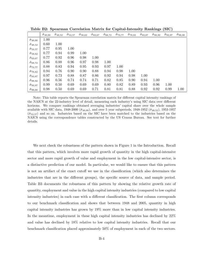
Table B2: Spearman Correlation Matrix for Capital-Intensity Rankings (SIC)�̂48;00 �̂48;52 �̂53;57 �̂58;62 �̂63;67 �̂68;72 �̂73;77 �̂78;82 �̂83;87 �̂88;92 �̂93;97 �̂98;00

�̂48;00 1:00�̂48;52 0:60 1:00�̂53;57 0:77 0:95 1:00�̂58;62 0:77 0:94 0:99 1:00�̂63;67 0:77 0:92 0:96 0:98 1:00�̂68;72 0:86 0:88 0:96 0:97 0:98 1:00�̂73;77 0:88 0:83 0:94 0:95 0:93 0:97 1:00�̂78;82 0:94 0:76 0:90 0:90 0:88 0:94 0:98 1:00�̂83;87 0:97 0:73 0:88 0:87 0:86 0:92 0:94 0:98 1:00�̂88;92 0:96 0:56 0:74 0:74 0:71 0:82 0:85 0:90 0:94 1:00�̂93;97 0:99 0:50 0:69 0:69 0:69 0:80 0:82 0:89 0:93 0:96 1:00�̂98;00 0:98 0:50 0:69 0:69 0:71 0:81 0:81 0:88 0:92 0:92 0:99 1:00

Note: This table reports the Spearman correlation matrix for di¤erent capital intensity rankings ofthe NAICS at the 22-industry level of detail, measuring each industry�s using SIC data over di¤erenthorizons. We compare rankings obtained averaging industries� capital share over the whole sampleavailable with SIC data, 1948-2000 (�̂48;00), and over 5 year subperiods, 1948-1952 (�̂48;52), 1953-1957(�̂53;57) and so on. Industries based on the SIC have been matched to the industries based on theNAICS using the correspondence tables constructed by the US Census Bureau. See text for furtherdetails.

We next check the robustness of the pattern shown in Figure 1 in the Introduction. Recall

that this pattern, which involves more rapid growth of quantity in the high capital-intensive

sector and more rapid growth of value and employment in the low capital-intensive sector, is

a distinctive prediction of our model. In particular, we would like to ensure that this pattern

is not an artifact of the exact cuto¤ we use in the classi�cation (which also determines the

industries that are in the di¤erent groups), the speci�c source of data, and sample period.

Table B3 documents the robustness of this pattern by showing the relative growth rate of

quantity, employment and value in the high capital intensity industries (compared to low capital

intensity industries) in each case with a di¤erent classi�cation. The �rst column corresponds

to our benchmark classi�cation and shows that between 1948 and 2005, quantity in high

capital intensity industries has grown by 19% more than in low capital intensity industries.

In the meantime, employment in these high capital intensity industries has declined by 22%

and value has declined by 18% relative to low capital intensity industries. Recall that our

benchmark classi�cation placed approximately 50% of employment in each of the two sectors.

B-4

The second and third columns report the same statistics, but using alternative cuto¤s so that

60% (column 2) and 40% (column 3) of total employment is in the industry grouping with

low capital intensity. In the former case, Accommodation and food services move into the low

capital intensity group. In the latter, Transport and warehousing move into the high capital

intensity group. In both cases, the general patterns remain very similar to the benchmark. For

example, with the 60% cuto¤, there is a 21% increase in the relative quantity of high capital

intensity industries, a 36% decline in their relative employment, and a 19% decline in their

value. With the 40% cuto¤, the relative increase in quantity is 44%, the relative decline in

employment is 19%, and the relative decline in value is 9%. Columns 4 and 5 show similar

results with the SIC data for the periods 1948-2000 and 1977-2000. We do not have quantity

data before 1977 with the SIC classi�cation, so the �rst row is missing in the fourth column.

The remaining rows in these columns are again similar to the benchmark, though when focusing

on the narrower sample of 1977-2000, the relative increase in quantity is only 2%. Finally, in

column 6 we report the results for the longer horizon 1929-2000. The only measure of value

added by industry available starting in 1929 is data on income by industry from the Historical

Statistics of the United States (the original source for these data is the BEA). The series of

full-time and part-time employees by industry in the NIPA tables also extends back to 1929. As

in column 4, we do not have quantity data, so that the �rst row of this column is missing. The

other two rows show a pattern consistent with the rest of the table, with a more rapid growth

of employment and value in the less capital-intensive industries than in more capital-intensive

industries.

B-5

Table B3: US Data robustness checks(1)

Benchmark(1948-2005)

(2)Cuto¤ 60%(1948-2005)

(3)Cuto¤ 40%(1948-2005)

(4)SIC Data(1948-2000)

(5)SIC Data(1977-2000)

(6)SIC Data(1929-2000)

growth %Y2=Y1

19% 21% 44% n:a: 2% n:a

growth %L2=L1

�22% �36% �19% �27% �20% �39%

growth %Y N2 =Y

N1

�18% �19% �9% �24% �9% �37%

Note: Column 1 in Table B4 reports the growth rate of quantity (quantity index for value added),employment (full-time and part-time employees) and value (value added) in the high capital intensitysector relative to the low capital intensity sector, constructed according to our benchmark classi�cationshown in Table B1. Columns 2 and 3 report the same statistics using alternative sectoral classi�cations,where the capital share cuto¤ for dividing industries into high and low capital intensity sectors ischosen to create a group of high-capital intensity industries including approximately 60% and 40%of total employment, instead of 50% as in the benchmark. The last three columns report the samestatistics for the benchmark sectoral classi�cation using the SIC data for di¤erent sample periods. Seetext for further details.

Finally, we have also looked for other sources of data to go back further than 1929. The

Historical Statistics of the United States provides a number of employment series, though in

most cases data are only available at a higher level of aggregation than the NIPA and the related

data we have used so far. The series with the �nest industry classi�cation in the Historical

Statistics of the United States is based on Sobek (2001) and covers only the time period 1910-

1990, which is only slightly earlier than the data we have reported in Table B3. These data are

available in 10 year intervals and use the 1950 Census industry classi�cation. Matching these to

the NAICS classi�cation, we computed employment growth in the high and low capital intensity

sectors.19 The results from this exercise are consistent with those in Table B3 and show that

employment in high capital intensity industries declines by about 10% relative to employment

in low capital intensity industries between 1910 and 1990. The remaining sources of data on

employment by industry have higher levels of aggregation, making the type of exercise we are

performing here more di¢ cult. One source of data on employment by industry is the Bureau

of Labor Statistics, which covers the period 1919-1999. However, a signi�cant fraction of the

industries are missing before 1939. We matched the industry classi�cation of this dataset to

the NAICS classi�cation,20 and computed employment growth in high and low capital intensity19For this exercise we dropped one of the 1950 census industry groups, �Transportation and Communication,�

because it combines two industries that are separated according to the NAICS classi�cation.20With this classi�cation, for the same reason as with the Sobek data, we had to drop the composite industry

�Transportation, Communication and Utilities�.

B-6

industries. The results show that employment in high capital intensity industries declines by

about 70% relative to employment in low capital intensity industries between 1939 and 1999.

The Historical Statistics of the United States also provides two other series, one from Lebergott

(1964) and Weiss (1992) covering the period 1800-1960, and the other from Lebergott (1984)

for 1900-1940. Unfortunately, given the more crude industry classi�cations, we were not able to

create a consistent match with to the NAICS classi�cations, especially with the former dataset.

It is also possible that the ranking of industries according to capital share, which appears to

be fairly stable in the postwar era, may be quite di¤erent when we go back before 1900. In any

case, using these data we were not able to obtain consistent patterns on relative employment

growth across high and low capital intensity industries. We believe that this re�ects the less

�ne industry aggregation in these data and the possible changes in the ranking according to

capital intensity, though it may also be due to data quality or because the patterns we have

documented for the past 80 years do not apply to the period before.

Additional References for Appendix B

The Historical Statistics of the United States (Millennial Edition Online), Editors: Carter

Susan B., Scott Sigmund Gartner, Michael R. Haines, Alan L. Olmstead, Richard Sutch, Gavin

Wright, New York : Cambridge University Press, c2006.

Sobek, Matthew �New Statistics on the U.S. Labor Force, 1850�1990,�Historical Methods

34 (2001): 71�87.

Lebergott, Stanley, Manpower in Economic Growth: The American Record since 1800,

McGraw-Hill, 1964.

Lebergott, Stanley, The Americans: An Economic Record, Norton, 1984.

Weiss, Thomas, U.S. Labor Force Estimates and Economic Growth, in Robert E. Gallman

and John Joseph Wallis, editors, American Economic Growth and Standards of Living before

the Civil War, University of Chicago Press, 1992.

B-7