Capacity Rights and Full Cost Transfer Pricing

Sunil Dutta

Haas School of Business

University of California, Berkeley

and

Stefan Reichelstein∗

Graduate School of Business

Stanford University

November 2017

Preliminary and Incomplete. Caveat Emptor

∗

Abstract: Capacity Rights and Full Cost Transfer Pricing

...........

1 Introduction

The transfer of intermediate products and services across divisions of a firm is fre-

quently valued at full cost. Surveys and textbooks consistently reported that, aside

from a market-based approach, cost-based transfer pricing is the most prevalent

method for both internal managerial and tax reporting purposes.1 One advantage

of full cost transfer pricing is that such a valuation approach is consistent with a

profit center organization that holds the individual divisions accountable for their

own profits.

Numerous case studies and managerial accounting textbooks have pointed out

that one drawback of full cost transfer pricing is that it may lead to sub-optimal

resource allocations. Double marginalization is one commonly articulated concern.

Accordingly, the buying division will internalize too high a charge for the product

in question because the measure of full cost includes fixed cost components that are

usually considered exogenous and sunk.2 In the HBS case study “Polysar Limited”

(Simons, 2000), the main issue with full cost transfer pricing is that the buying

division tends to reserve too much production capacity because it faces uncertain

demand for its own product, yet the full cost charges are only applied to capacity

that is actually utilized.

The objective of this paper is to delineate environments in which full cost transfer

pricing “works”, that is, it is part of an effective divisional performance measurement

system. In the setting of our model, managers decide on both the initial acquisition of

productive capacity and its utilization in subsequent periods, once operational uncer-

tainty has been resolved.3 For simplicity, our model considers two divisions that are

each selling a product in separate markets. Due to technical expertise, the upstream

1See, for instance, Ernst & Young (1993)Tang (2002), Feinschreiber and Kent (2012), Pfeiffer etal. (2009), and Zimmerman (2016)

2For instance, the issue of double marginalization features prominently in Baldenius et al. (1997),Datar and Rajan (2014) and Zimmerman (2016).

3In effect, the acquisition of capacity creates a real option that may subsequently be put toefficient use.

1

division installs and maintains all productive capacity. It also produces the output

sold by the downstream division. For performance evaluation purposes, the upstream

division is therefore viewed as an investment center, while the downstream division,

having no operating assets, is merely a profit center. The periodic transfer payments

from the upstream to the downstream division depend on the initial capacity choices

and the current production levels. We refer to a transfer pricing rule as a full cost

rule if the present value of all transfer payments is equal to the present value of all

cash outflows associated with the capacity assigned to the downstream division and

all subsequent output services rendered to that division.4 That balancing constraint

must not necessarily hold as an identity but only on the equilibrium path.

Our criterion for incentive compatibility follows earlier work on goal congruent

performance measures such as Rogerson (1997), Dutta and Reichelstein (2002), Balde-

nius et al.(2007) and Nezlobin et al.(2015). Accordingly the divisional performance

measures must in any specific time period be congruent with the objective of maxi-

mizing firm value. Put differently, regardless of the weight that a manager attaches to

his/her divisional performance measures in any given period, it must provide an in-

centive to choose the upfront capacity level efficiently and to maximize the attainable

contribution margin in subsequent periods.

We distinguish the two alternative scenarios of dedicated and fungible capacity,

depending on whether the divisions’ products can share the same capacity assets.

In the dedicated capacity setting, each division is given unilateral capacity rights.

As a consequence, there is no strategic interaction between the divisions and the

upstream division merely becomes a service provider for the downstream division.

Under certain conditions, the naive full cost transfer pricing rule, as featured for

instance in the Polysar case, can be modified to obtain a goal congruent solution.

Essential to this finding is that the buying division now also faces excess capacity

4In particular, a two-part pricing rule that charges in a lump sum fashion for capacity in eachperiod in addition to variable charges, based on actual production volumes, will be considered afull-cost transfer price.

2

charges.5 While such excess capacity charges will not be imposed in equilibrium, the

potential threat is sufficient to correct for the bias inherent in naive full cost transfer

pricing.

In the dedicated capacity scenario, we identify a class of production and informa-

tion environments where a suitable variant of full cost transfer pricing induces efficient

outcomes. We find the preferred transfer pricing rule varies depending on whether

the value of capacity is expected to change over time and whether, given an efficient

capacity choice in the first place, there is a significant probability that capacity will

remain partly idle.6 Common to these pricing rules is that the fixed cost charges for

capacity must be equal to what earlier literature has referred to as the “user cost of

capital” or the “marginal cost of capacity.” 7

When the two products in question can share the same capacity installation, it

suggests itself to allow the divisions to negotiate ex-post an efficient utilization of the

available capacity. such an an arrangement still still leaves the issue of coordinating

the initial capacity acquisition. If that decision were to be delegated to the upstream

division, in its role as an investment center, the resulting outcome would generally

entail underinvestment. The reason is that the upstream division would anticipate

not earning the full expected return on its investment because gains from the opti-

mized total contribution margin would be shared in the negotiation between the two

divisions, while the initial acquisition cost would be considered sunk.8 Our findings

5Our solution here is consistent with prescriptions in the managerial accounting literature on howto allocate the overhead costs associated with excess capacity, e.g., Kaplan (2006) and Martinez-Jerez(2007).

6We refer to this condition as the “limited volatility condition.” It plays a central role in Re-ichelstein and Rohlfing-Bastian (2015) in characterizing the relevant cost to be imputed for capacityexpansion decisions.

7In contrast to our framework here, the derivation of the user cost of capital has been derivedin models with overlapping investments in an infinite horizon setting, e.g., Arrow (1964), Rogerson(2008), Rajan and Reichelstein (2009) and Reichelstein and Sahoo (2017).

8Even though investments are verifiable in our model, the hold-up problem that arises when onlythe upstream division makes capacity investments is essentially the same as in earlier incompletecontracting literature. One branch of that literature has explored how transfer pricing can alleviatehold-up problems when investments are “soft” (unverifiable); see, for example, Baldenius et al.(1999),Edlin and Reichelstein (1996), Sahay (2000) and Pfeiffer et al. (2009).

3

show that under certain conditions the coordination problem associated with the ini-

tial capacity choice can be resolved by giving both divisions the the unilateral right

to reserve capacity and charging the downstream division for its reservation through

full cost transfer prices.

An alternative, and more robust, coordination mechanism is obtained in the fungi-

ble capacity scenario if the downstream division must obtain approval for any capacity

it wants to reserve for its own use. The upstream division then becomes essentially

a “gatekeeper” that will agree to let the downstream division reserve capacity for

itself in exchange for a steam of lump-sum payments determined through initial ne-

gotiation. The upstream division will then have an incentive to invest in additional

capacity on its own up to the efficient level. The resulting mechanism can be viewed

as a hybrid cost-based/negotiated transfer pricing rule such that the gatekeeper is

charged the full cost of the total capacity acquired and total output produced.

This paper is most closely related to three earlier studies. Dutta and Reichelstein

(2010) also examine full cost transfer pricing in a model where capacity choices are

endogenous. An crucial restriction of their framework, though, is that the firm does

not incur any variable operating costs. As a consequence, capacity will always be

fully utilized regardless of the investment levels. The issue of potential excess ca-

pacity arises in the more recent studies of Reichelstein and Rohlfing- Bastian (20150

and Baldenius, Nezlobin and Vaysman (2016). However, incentive issues are absent

in the work of Reichelstein and Rohlfing-Bastian (2015) examining capacity decisions

entirely from a planning perspective. Baldenius et al. (2016) study managerial per-

formance evaluation for a single manager in a setting where capacity may remain idle

in unfavorable states of the world.

The remainder of the paper proceeds as follows. The basic model is described

in Section 2. Section 3 examines a setting in which the divisions’ products require

different production facilities and therefore capacity is dedicated. Propositions 1 - 4

delineate environments in which full cost transfer pricing can induce the divisions to

choose initial capacity levels and subsequent production levels that are efficient from

4

the overall firm perspective. Section 4 considers the alternative arrangement in which

capacity is fungible and can be traded across across divisions. Propositions 5 and 6

demonstrate the need for allowing the downstream division to secure capacity rights

for itself initially, even if the entire available capacity can be reallocated through

subsequent negotiations in subsequent periods. We conclude in Section 5.

2 Model Description

Consider a vertically integrated firm comprised of two divisions and a central office.

Both divisions sell a marketable product (possibly a service) in separate and unrelated

markets. In order for either division to deliver its product in subsequent periods, the

firm needs to make upfront capacity investments. Because of technical expertise,

only the upstream division (Division 1) is in a position to install and maintain the

productive capacity for both divisions. That division is also assumed to carry out the

production of both products and therefore incurs all periodic production costs.9 Our

analysis considers an organizational structure which views the upstream division as an

investment center whose balance sheet reflects the historical cost of the initial capacity

investments. In that sense, the upstream division acquires economic “ownership” of

the capacity related assets.

Capacity could be measured either in hours or the amount of output produced.

New capacity is acquired at time t = 0. Our analysis considers the two distinct

scenarios of dedicated and fungible capacity. In the former scenario, the two products

are sufficiently different so as to require separate production facilities. With fungible

capacity, in contrast, both products can share the same capacity infrastructure. The

upfront cash expenditure for one unit of capacity for Division i is vi in the dedicated

capacity setting. If division i acquires ki units of capacity, it has the option to produce

up to ki units of output in each of the next T periods.10 In case of fungible capacity,

9It is readily verified that our findings would be unchanged if the upstream division were totransfer an intermediate product which is then completed and turned into a final marketable productby the downstream division.

10We thus assume that physical capacity does not diminish over time, but instead follows the

5

the unit cost of acquiring capacity is v, allowing either division to produce one unit

of its product in any of the next T periods.

The actual production levels for Division i in period t are denoted by qit. Aside

from requisite capacity resources, the delivery of one unit of output for Division i

requires a unit variable cost of wit in period t. These unit variable costs are anticipated

upfront by the divisional managers with certainty, though they may become known

and verifiable to the firm’s accounting system only when incurred in a particular

period. The corresponding contribution margins are given by:

CMit(qit, εit) = xit ·Ri(qit, εit)− wit · qit.

The first term above, xit·Ri(qit, εit), denotes division i’s revenues in period t with xit ≥0 representing intertemporal parameters that allow for the possibility of declining, or

possibly growing, revenues over time.

In addition to varying with the production quantities qit, the periodic revenues

are also subject to (one-dimensional) transitory shocks εit. These random shocks

are realized at the beginning of period t before the divisions choose their output

levels for the current period, and prior to any capacity trades in the fungible capacity

setting. The εit are realized according to density functions fi(·) with support on the

interval [εi, εi]. Unless stated otherwise, the transitory shocks {εit} are independently

distributed across time; i.e., Cov(εit, εiτ ) = 0 for each t 6= τ , though in any given

period these shocks may be correlated across the two divisions; i.e., it is possible to

have Cov(ε1t, ε2t) to be non-zero.

The exact shape of the revenue revenue functions, Ri(qit, εit), is private information

of the divisional managers. These revenue functions are assumed to be increasing and

concave in qit for each i and each t. At the same time, the marginal revenue functions:

R′

i(q, εit) ≡∂Ri(q, εit)

∂q

are assumed to be increasing in εit.

“one-hoss shay” pattern, commonly used in the capital accumulation and regulation literature. See,for example, Rogerson (2008) or Nezlobin, Rajan and Reichelstein (2012).

6

In any given period, the actual production quantity for a division may differ

from its initial capacity rights for two reasons. First, for an unfavorable realization

of the revenue shock εit, a division may decide not to exhaust the entire available

capacity because otherwise marginal revenues would not cover the incremental cost

wit. Second, in the case of fungible capacity, a division may want to yield some of its

capacity rights to the other division if that division has a higher contribution margin.

Our model is in the tradition of the earlier goal congruence literature which does

not explicitly address issues of moral hazard and managerial compensation. Instead

the focus is on the choice of goal congruent performance measures for the divisions.

Following this literature, we assume that each divisional manager is evaluated accord-

ing to a performance measures πit in each of the T time periods.. The downstream di-

vision, which has only operational responsibilities for procuring and selling output, is

treated as a profit center whose performance measure is measured by operating profit.

In contrast, the upstream division also has control over capacity assets. Hence, it is

viewed as an investment center with residual income as its performance measure.11

The remaining design variables of the internal managerial accounting system then

consist of divisional capacity rights, depreciation schedules, and the transfer pricing

rule.

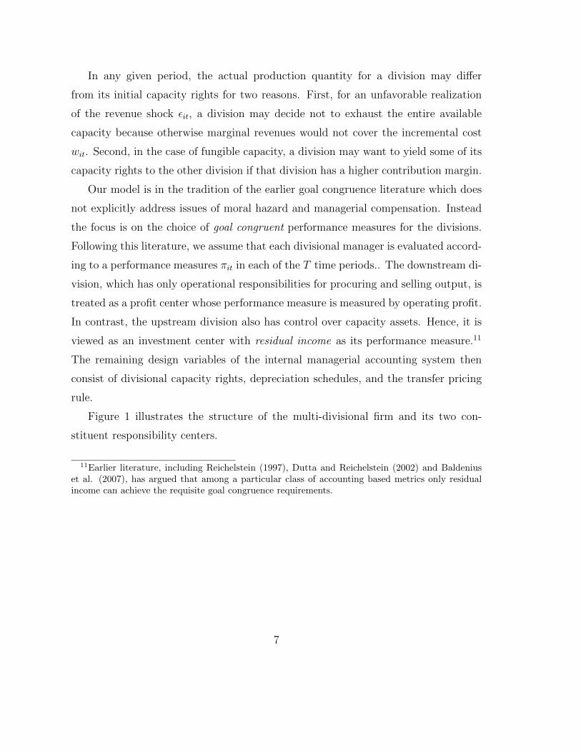
Figure 1 illustrates the structure of the multi-divisional firm and its two con-

stituent responsibility centers.

11Earlier literature, including Reichelstein (1997), Dutta and Reichelstein (2002) and Baldeniuset al. (2007), has argued that among a particular class of accounting based metrics only residualincome can achieve the requisite goal congruence requirements.

7

Income StatementExternal Revenue

- TPIncome

Upstream Division

Downstream Division

2tq

TP

Income StatementExternal Revenue

- Operating Costs- Depreciation- Capital Charge+ TP

Income

Balance Sheet

Capacity Assets

Multi-Divisional Firm

Figure 1: Divisional Structure of the Firm

The downstream division’s performance measure (i.e., its operating income) in

period t is given by

π2t = Inc2t = x2t ·R2(q2t, ε2t)− TPt(k2, q2t),

where TPt(k2, q2t) denotes the transfer payment to the upstream division in period t

for securing k2 units of capacity and obtaining q2t units of output in period t. The

residual income measure for the upstream division is represented as:

π1t = Inc1t − r ·BVt−1, (1)

where BVt denotes book value of capacity assets at the end of period t, and r denotes

the firm’s cost of capital. The corresponding discount factor is denoted by γ ≡(1 + r)−1. The residual income measure in (1) depends on two accruals: the transfer

8

price received from the downstream division and the current depreciation charges

corresponding to the initial capacity investments. Specifically,

Inc1t = x1t ·R1(q1, ε1t)− w1t · q1t − w2t · q2t −Dt + TPt(k2, q2t),

where Dt is the total depreciation expense in period t. Let dit represent the depre-

ciation charge in period t per dollar of initial capacity investment undertaken for

Division i. Thus:

Dt = d1t · v1 · k1 + d2t · v2 · k2.

The depreciation schedules satisfy the usual tidiness requirement that∑T

τ=1 diτ = 1;

i.e, the depreciation charges sum up to an asset’s historical acquisition cost over its

useful life. Book values evolve according to the simple iterative dynamic: BVt =

BVt−1 −Dt, with BV0 = v1 · k1 + v2 · k2 and BVT = 0.

Under the residual income measure, the overall capital charge imposed on the

upstream division is the sum of depreciation charges plus imputed interest charges.

Given the depreciation schedules {dit}Tt=1, the overall capital charge becomes:

Dt + r ·BVt−1 = z1t · v1 · k1 + z2t · v2 · k2, (2)

where zit ≡ dit + r · (1 −∑t−1

τ=1 diτ ). It is well known from the general properties of

the residual income metric that regardless of the depreciation schedule, the present

value of the zit is equal to one; that is,∑T

t=1 zit · γt = 1 (Hotelling, 1925).

The manager of Division i is assumed to attach non-negative weights {uit}Ti=1 to

her performance measure in different time periods. The weights ui = (ui1, ..., uiT )

reflect both the manager’s discount factor as well as the bonus coefficients attached

to the periodic performance measures. Manager i’s objective function can thus be

written as∑T

t=1 uit · E[πit]. A performance measure is said to be goal congruent if

it induces equilibrium decisions that maximize the present value of firm-wide cash

flows. Consistent with the earlier goal congruence literature, we impose the criterion

9

of strong goal congruence, which requires that managers have incentives to make

efficient production and investment decisions for any combination of the coefficients

uit ≥ 0. Strong goal congruence requires that desirable managerial incentives must

hold not only over the entire planning horizon, but also on a period-by-period basis.

That is, each manager must have incentives to make efficient production and capacity

decisions even if that manager were only focused on maximizing her performance

measure πiτ in any given single period τ .

The criterion of strong goal congruence may be combined with alternative notions

of a non-cooperative equilibrium between the two divisions, e.g., dominant strate-

gies or Nash equilibrium. An additional property that we highlight in some of our

subsequent results is the notion of autonomous performance measures. We refer to

a performance measurement system as autonomous if it has the property that each

manager’s performance measure is unaffected by the decisions made by the other

manager. Clearly, this criterion of autonomy implies that the divisions must have a

dominant strategy.

3 Dedicated Capacity

When capacity cannot be traded periodically across the two divisions because the

products in question require different capacity infrastructures, there is effectively no

intra-firm coordination problem. The analysis of this section focuses on identifying

the depreciation schedules and transfer pricing rules that provide incentives for the

divisional managers to choose efficient levels of capacity upfront and make optimal

production decisions in subsequent periods. The following time-line illustrates the

sequence of events at the initial investment date and in a generic period t.

10

Figure 2: Sequence of Events in the Dedicated Capacity Scenario

If a central planner had full information regarding future revenues, the optimal

investment decisions (k1, k2) would be chosen so as to maximize the net present value

of the firm’s expected future cash flows

Γ(k1, k2) = Γ1(k1) + Γ2(k2), (3)

where

Γi(ki) =T∑t=1

Eεi [CMit(ki|xit, wit, εit)] · γt − vi · ki, (4)

and CMit(·) denotes the maximized value of the expected future contribution margin

in period t:

CMit(ki|xit, wit, εit) ≡ xit ·Ri(qoit(ki, ·), εit)− wit · qoit(ki, ·),

with

qoit(ki, ·) = argmaxqit≤ki

{xit ·Ri(qi, εit)− wit · qi}.

The notation qoit(ki, ·) above is short-hand for the sequentially optimal quantity

qoit(ki, εit, xit, wit) that maximizes the divisional contribution margin in period t, given

the initial capacity choice, current revenues and variable costs and the realization

of the current shock εit. To avoid laborious checking of boundary cases, we assume

throughout our analysis that the marginal revenue at zero always exceeds the unit

variable cost of production. Formally,

R′i(0, εit)− wi > 0

11

for all realizations of εit.

3.1 Stationary Environments

One significant simplification for the resource allocation problem we study obtains if

firms anticipate that the economic fundamentals are, at least in expectation, identical

over the next T periods. Formally, an environment is said to be stationary if xit = 1,

wit = wi and the {εit} are i.i.d. for each i. For the setting of stationary environments,

we drop subscript t from CMit(·) and qoit(·). The result below characterizes the efficient

capacity levels, koi , for this setting.

Lemma 1 Suppose capacity is dedicated and the divisional environments are station-

ary. If the optimal capacity level, koi , is greater than zero, it is given by the unique

solution to the equation:

Eεi

[R

′

i(qoi (k

oi , wi, εit), εit)

]= ci + wi, (5)

where

ci =vi∑Tt=1 γ

t. (6)

Proof: All proofs are in the Appendix.

Reichelstein and Rohlfing-Bastian (2015) refer to ci as the unit cost of capacity.

It takes the initial acquisition expenditure for one unit of capacity and “levelizes”

this expenditure by dividing it through the annuity factor of $1 paid over T periods;

i.e.,∑T

t=1 γt. It is readily verified that ci is the price that a hypothetical supplier

would charge for renting out capacity for one period of time if the rental business

were constrained to break even. Lemma 1 says that the optimal capacity level, koi ,

is such that the expected marginal revenue at the sequentially optimal production

levels, qoi (koi , ·) is equal to the sum of the unit cost of capacity c and the variable

12

cost wi. We shall subsequently refer to this sum, ci + wi, as the full cost per unit of

output.12

It is readily verified that a necessary and sufficient condition for koi to be positive

is:

Eεi [R′i(0, εit)] > ci + wi. (7)

For future reference, we also note that the result in Lemma 1 can be restated as

follows: the optimal capacity level, koi > 0 is such that the marginal expected con-

tribution margin in all subsequent periods must be equal to the unit cost of capacity

ci:

Eεi

[CM

′

i (koi , |wi, εit)

]= ci,

where CM′i (k

oi , wi, εit) ≡ R

′i(q

oi (k

oi , ·), εit)− wi.

In the context of our model, one representation of full cost transfer pricing is

that the downstream division is charged in the following manner for intra-company

transfers:

1. Division 2 has the unilateral right to reserve capacity at the initial date.

2. Division 2 can choose the quantity, q2t, to be transferred in each period subject

to the initial capacity limit.

3. In period t, Division 2 is charged the full cost of output delivered, that is:

TPt(k2, q2) = (w2 + c2) · q2t.

This variant of full cost transfer pricing is exactly the one featured in the Harvard

case study “Polysar” (Simons, 2000). The downstream division is effectively charged

12As observed in Reichelstein and Rohlfing-Bastian (2015), ci+wi will generally exceed the tradi-tional measure of full cost as conceptualized in managerial accounting. The reason is that the lattermeasure does not include the imputed interest charges for capital. For instance, if the depreciationcharges are uniform, the traditional measure of full cost is given by vi

T + wi, which is clearly lessthan vi∑T

t=1 γt + wi ≡ ci + wi.

13

for the reserved capacity only if it actually utilizes that capacity. The upshot of that

case study is that the buying division has an incentive to reserve too much capacity

upfront, since such a strategy preserves the buying division’s option to meet market

demand if it turns out to be strong. On the other hand, the buying division incurs no

penalty for idling capacity if the ex-post market conditions turn out to be unfavorable.

In contrast to the conclusion from the Polysar case study, Dutta and Reichelstein

(2010) show that the above form of full cost transfer pricing generates efficient ca-

pacity investment incentives and achieve goal congruence in the dedicated capacity

setting. We note, however, that their result critically relies on their assumption of

no variable production costs (i.e., w2 = 0), and hence the issue of capacity under-

utilization never arises in their setting. In the analysis of Dutta and Reichelstein

(2010), divisions are thus effectively charged for the amount of capacity they reserve

and this choice ex-post always coincides with the actual production levels.

Another issue with the variant of cost-based transfer pricing described above is

that unless q2t = k2 in each period, the discounted value of the transfer pricing

charges is not equal to the total discounted cost comprising capacity investment and

subsequent operating costs. While this is arguably not a major issue for an internal

accounting rule, it is nonetheless a desirable balancing constraint. Accordingly, we

introduce the following criterion:

Definition A transfer pricing rule is said to be a full cost pricing rule if, in equilib-

rium:T∑t=1

TPt(k2, q2t) · γt = v2 · k2 +T∑t=1

w2t · q2t · γt

The qualifier “in equilibrium” in the preceding definition refers to the notion that

the transfer payments needs to be balanced only for the equilibrium investment and

operating decisions. The specific notion of equilibrium will vary with the particular

setting considered, specifically whether capacity is dedicated or fungible.

To deter divisional managers from reserving “excessive” amounts of capacity, one

possibility is to impose excess capacity charges. In addition to the full cost of units

14

delivered, the buying decision will then be charged in proportion to the amount of

capacity not utilized at some rate µ. A full cost transfer pricing rule subject to the

excess capacity charges will entail the following transfer payments:

TPt(k2, q2t) = (w2 + c2) · q2t + µ · (k2 − q2t). (8)

In any given period, the available capacity will generally be fully utilized in good

states of the world with high marginal revenues (high realizations of εit). On the other

hand, capacity may be left idle under unfavorable market conditions (low realizations

of εit). To state our first formal result, we introduce a notion of limited volatility in

the revenue shocks εit such that capacity will be fully utilized on the equilibrium path.

Following Reichelstein and Rohlfing-Bastian (2015), we say that the limited volatility

condition holds if qoi (koi , ·) = koi for all realizations of εit where koi again denotes the

efficient capacity level. We note that the limited volatility condition will be met if

and only if, the inequality:

R′

i(koi , εit)− wi ≥ 0

holds for all realizations of εit. Intuitively, the available capacity will always be

exhausted in environments with relatively low volatility in terms of the range and

impact of the εit, or alternatively, if the unit variable cost, wi, is small relative to the

full cost, wi+ci. The limited volatility condition is thus a joint condition on the range

of ex-post uncertainty and the relative magnitude of the unit variable cost relative to

the full cost.13

Proposition 1 Suppose capacity is dedicated, the environment is stationary, and the

limited volatility condition holds. Full cost transfer pricing subject to excess capacity

charges, as given in (8), then achieves strong goal congruence provided µ ≥ c2 and

capacity assets are depreciated according to the annuity rule.

13The jointness of this condition is apparent in the setting of Reichelstein and Rohlfing-Bastian(2015) who impose the separability condition Ri(qi, εit) = εit · Ri(qi) with E(εit) = 1. It is readilyverified that with multiplicative separability, the limited volatility conditions holds if and only ifεit ≥ wi

wi+ci.

15

Excess capacity charges restore the efficiency of full cost transfers for three reasons.

First, the classic double marginalization problem does not arise as the downstream

division will internalize an incremental production cost of w2 + c2 − µ < w2. Second,

the buying division will not have a short-run incentive to overproduce because the

limited volatility condition ensures that the division would have exhausted the efficient

capacity level, koi for all realizations of εit if it had imputed an incremental cost of wi

per unit of output. The downstream division will therefore also exhaust the available

capacity in all states of the world if it imputes a marginal cost less than w2. Finally, in

making its initial capacity choice, the buying division will only internalize the actual

unit cost of capacity, c2, because, given the limited volatility condition, there will be

no excess capacity charges in equilibrium. We note parenthetically that there would

have been no need for excess excess capacity charges if either there is no periodic

volatility in divisional revenues (the εit are always equal to their average values) or

there are no incremental costs to producing output (w2 = 0).

Full cost transfer pricing subject to suitably chosen excess capacity charges pro-

vides the divisional managers with dominant strategy choices with regard to both

their initial capacity and subsequent production decisions. The annuity deprecia-

tion schedule ensures that the downstream division’s choices are merely pass-through

from the perspective of the upstream division’s performance measure because, in

equilibrium, the transfer payment from Division 2 is precisely equal to the sum of

depreciation charges, imputed capital charges, and variable production costs incurred

by Division 1. Therefore, the performance evaluation system satisfies our criterion of

autonomy.

We note that for the above goal congruence result it is essential that the excess

capacity charge, µ, be at least as large as the unit cost of capacity c2. Otherwise,

the issues observed in connection with the transfer pricing policy in the Polysar case

(where µ = 0) would resurface. Specifically, there would be a double marginalization

problem in each period, since the downstream division would impute a marginal cost

higher than w2. In addition, this division would have incentives to procure excessive

16

capacity because it is charged for the capacity only when actually utilized.

If the limited volatility condition for the buying division is not met, it will be

essential to precisely calibrate the excess capacity charges. The obvious choice here

is µ = c2, which results in the two-part full cost transfer pricing rule:

TPt(k2, q2t) = c2 · k2 + w2 · q2t (9)

Clearly, this pricing rule satisfies our criterion of a full cost transfer pricing rule

insofar as the sum of the discounted transfer payments are identically equal to the

initial capacity acquisition cost plus the discounted sum of the subsequent variable

production costs. The transfer pricing rule in (9) also ensures that each division

manager’s performance measure is autonomous.

Proposition 2 With dedicated capacity and a stationary environment, the two-part

full cost transfer pricing rule in (9) achieves strong strong congruence, provided ca-

pacity assets are depreciated according to the annuity rule.

With significant volatility, any excess capacity charge µ exceeding c2 would induce

the downstream division to (i) use too much of the available capacity and (ii) secure

an inefficient amount of capacity upfront. In fact, we conjecture that, absent any

restrictions on the amount of volatility, the two-part transfer pricing mechanism in

(9) is unique among the class of linear transfer pricing rules of the form TPt(k2, q2t) =

a1 · k2 + a2 · q2t; that is a1 = c2 and a2 = w2 are not only sufficient but also necessary

for strong goal congruence.

3.2 Non-Stationary Environments

We have thus far restricted our analysis to stationary environments in which each

division’s costs and expected revenues are identical across periods. In this subsec-

tion, we investigate depreciation and transfer pricing rules that can achieve strong

17

goal congruence for certain non-stationary environments. The following result char-

acterizes the efficient capacity choices by generalizing Lemma 1 for non-stationary

environments:

Lemma 2 If capacity is dedicated and the optimal capacity level, koi , in (5) is greater

than zero, it is given by the unique solution to the equation:

T∑t=1

Eεit

[xit ·R

′

i(qoit(k

oi , εit, xit, wit), εit)

]· γt = vi + wi (10)

where

wi =T∑t=1

wit · γt.

It is readily seen that the claim in Lemma 2 reduces to that in Lemma 1 whenever

xit = 1, wit = wi and {εit} are i.i.d. Beginning with the work of Rogerson (1997),

earlier work on goal congruent performance measures has shown that if the revenues

attained vary across time periods, proper intertemporal cost allocation of the initial

investment expenditure requires that depreciation be calculated according to the rel-

ative benefit rule rather than the simple annuity rule. This insight extends to the

setting of our model provided the variable costs of production change in a coordi-

nated fashion over time. Formally, the relative benefit depreciation charges are the

ones defined by the requirement that the overall capital charge in period t (i.e., the

sum of depreciation and imputed interest charges), as introduced in equation (2), be

given by:14

zit ≡xit∑T

τ=1 xiτ · γτ

14As pointed out by earlier studies, the corresponding relative benefit depreciation charges willcoincide with straight-line depreciation if the xit decline linearly over time at a particular rate(Nezlobin et al. 2015).

18

Corollary to Proposition 2: If capacity is dedicated and wit = xit · wi, a two-part

full cost transfer pricing rule of the form

TPt(k2, q2t) = z2t · v2 · k2 + w2t · q2t

achieves strong strong congruence, provided capacity assets are depreciated according

to the relative benefit depreciation rule.

The preceding result generalizes the result in Proposition 2 to a class of non-

stationary environments in which expected revenues and variable costs are different

across periods. However, the settings to which the above result applies appear rather

restrictive. Specifically, the result requires that intertemporal variations in periodic

revenues and variable production costs follow identical patterns (i.e., wit = xit · wi).With limited volatility, the following result below shows that the finding of Propo-

sition 2 can be extended to a broader class of non-stationary environments.

Proposition 3 Suppose capacity is dedicated, the limited volatility condition holds,

and the {εit} are i.i.d. The full cost transfer pricing rule

TPt(k2) = z2t · (v2 + w2) · k2

achieves strong goal congruence, provided the anticipated variable production costs of

each division, wi · ki, are capitalized and the divisional capacity assets, (vi + wi) · kiare depreciated according to the respective relative benefit rule.

The above transfer pricing rule does not charge the downstream division for actual

variable costs incurred in connection with the actual production volume. Instead, the

buying division is charged for the “budgeted” variable costs that will be incurred in

future time periods assuming that the initially chosen capacity chosen will be fully

exhausted in all future periods. Such a policy is indeed efficient if (i) the limited

volatility condition holds, and (ii) the downstream division has an incentive to choose

the efficient capacity level in the first place. For the above transfer pricing rule, the

divisional profit of the downstream division in any period τ is proportional to:

19

T∑t=1

Eε2 [x2t ·Ri(k2, εi)] · γt − (v2 + w2) · k2,

which coincides with the firm’s overall objective function for any k2 ≤ ko2.

We note that TPt(k2) = z2t · (v2 + w2) · k2 is a full-cost transfer pricing rule

because in equilibrium, Division 2 initially procures ko2 and subsequently exhausts

the available capacity. However, this transfer pricing rule clearly no longer satisfies

the criterion of being autonomous because the upstream division’s variable costs of

production are balanced by the transfer payments received from the buying division

only over the entire T period horizon, but not on a period-by-period basis.

To extend the preceding result to environments where the limited volatility con-

dition may not be satisfied, we adopt the simplified decision structure in Baldenius,

Nezlobin and Vaysman (2016, Proposition 1), where the set of possible investment

levels is binary. Specifically, suppose that each division chooses whether to install a

specific amount of capacity ki or not; i.e., ki ∈ {0, ki}. Suppose further that each divi-

sion’s revenue function Ri(·, εit) is publicly known. Each divisional manager’s private

information is a one-dimensional parameter θi which affects the probability distribu-

tions of εit. Specifically, θi is assumed to shift the conditional densities f(εit|θi) in the

sense of first-order stochastic dominance.

The simplification with a binary choice set is that the accrual accounting rules,

i.e., depreciation schedule and transfer pricing rule, only need to separate the types of

θi for whom capacity investment is in the firm’s interest from those types for whom it

is not. Accordingly, consider the threshold type, θ∗i , where the firm is just indifferent

between investing and not investing:

Γi(ki|θ∗i ) =T∑t=1

Eεi[CMit(ki, xit, wit, εit)|θ∗i )

]· γt − vi · ki = 0. (11)

As before, CMit(·) denotes the maximized value of the expected future contribution

margin in period t:

20

CMit(ki, xit, wit, εit) ≡ xit ·Ri(qoit(ki, ·), εit)− wit · qoit(ki, ·).

Following the terminology in Baldenius, Nezlobin and Vaysman (2016), we refer

to the Relative Expected Optimized Benefit (REOB) cost allocation rule as:

zit =Eεi[CMit(ki, xit, wit, εit)|θ∗i

]∑Tτ=1 Eεi

[CMit(ki, xiτ , wiτ , εiτ )|θ∗i

]· γτ .

The REOB rule is effectively the relative benefit rule for the pivotal type, θ∗i .15

Proposition 4 Suppose the set of feasible capacity investment choices is binary and

the future realizations of εit are drawn according to conditional densities f(εit|θi) such

that θi shifts f(εit|θi) in the sense of first-order stochastic dominance. The full-cost

transfer pricing rule

TPt(k2, q2t) = z2t · v2 · k2 + w2t · q2t

then achieves strong goal congruence, provided capacity assets are depreciated accord-

ing to the REOB rule.

Like the two-part tariff in Proposition 2, the transfer pricing rule identified in the

above finding is a full-cost transfer pricing rule which satisfies the criterion of being

autonomous. To see that it achieves goal congruence, we note that by definition of

the threshold type, the overall NPV of capacity investment is zero at θi = θ∗i :

T∑τ=1

Eεi[CMit(ki, xiτ , wiτ , εiτ )|θ∗i

]· γτ = vi · ki.

If θi moves the probability distributions of εit in the sense of first-order stochastic

dominance, the NPV corresponding to any εit will be greater than zero if and only if

θi > θ∗i , because CMit(·) is increasing in εit. Consider now the downstream division’s

incentive to invest. If that division were to focus exclusively on its profit measure in

period t, 1 ≤ t ≤ T , it would be seek to maximize:

15Clearly, this rule reduces to annuity depreciation in a stationary environment.

21

Eε2 [π2(θ2)] ≡ Eε2[CM2t(k2, x2t, w2t, ε2t)|θ2

]− z2t · v2 · k2.

By construction of the REOB rule, Eε2 [π2(θ2)] ≥ 0 if and only if

Eε2[CM2t(k2, x2t, w2t, ε2t)|θ2

]≥ Eε2

[CM2t(k2, x2t, w2t, ε2t)|θ∗2

],

which will be the case if and only if θ2 ≥ θ∗2. Goal congruence for the upstream

division follows from a parallel argument.

4 Fungible Capacity

In contrast to the scenario considered thus far, where the products or services provided

by the two divisions required different production assets, we now consider the plausible

alternative of fungible capacity. Accordingly, the production processes of the two

divisions have enough commonalities and the demand shocks εt are realized sufficiently

early in each period, so that the initial capacity choices can be reallocated across the

two divisions. The following time-line illustrates the sequence of events at the initial

investment date and in a generic period.

Figure 3: Sequence of Events in the Fungible Capacity Scenario

The following analysis focuses at first on stationary environments. We use the

vector notation: w ≡ (w1, w2), and εt ≡ (ε1t, ε2t). With fungible capacity, the optimal

investment from a firm-wide perspective is the one maximizing total expected future

cash flows:

22

Γ(k) =T∑t=1

Eεt [CM(k|θ, w, εt)] · γt − v · k (12)

where CM(·) denotes the maximized value of the aggregate contribution margin in

period t. That is,

CM(k|w, εt) ≡2∑i=1

[Ri(q∗i (k, ·), εit)− w · q∗i (k, ·)],

where

(q∗1(k, ·), q∗2(k, ·)) = argmaxq1+q2≤k

{2∑i=1

[Ri(qi, εit))− wi · qi]}.

As before, the notation q∗i (k, ·) is short-hand for q∗i (k, w, εt).

Provided the optimal quantities q∗i (k, ·) are both positive, the first-order condition:

R′

1(q∗1(k, ·), ε1t)− w1 = R′

2(q∗2(k, ·), ε2t)− w2 (13)

must hold. Allowing for corner solutions, we define the shadow price of capacity in

period t, given the available capacity k, as follows:

S(k|w, εt) ≡ max{R′

1(q∗1(k, ·), ε1t)− w1, R′

2(q∗2(k, ·), ε2t)− w2}. (14)

Thus, the shadow price of capacity identifies the maximal change in periodic contri-

bution margin that the firm can obtain from an extra unit of capacity.16 We note

that S(·) is increasing in εit, but decreasing in wi and k.

Lemma 3 Suppose capacity is fungible and the divisional environments are station-

ary. The optimal capacity level, k∗, is given by the unique solution to the equation:

Eε [S(k∗|w, εit)] = c, (15)

16The assumption that R′

i(0, εit) ≥ wi for all εit ensures that the shadow price of capacity is alwaysnon-negative.

23

where

c =v∑Tt=1 γ

t. (16)

We next examine the divisions’ capacity investment choices in the decentralized

setting. Given the finding in Proposition 2, it is natural to consider whether the two-

part full cost transfer pricing rule in (9) can induce goal congruence if the divisions are

allowed to renegotiate the initial capacity rights after realization of revenue shocks εt

in each period. To examine this, suppose that the downstream division has procured

initial rights for k2 units of capacity, the upstream division has installed k1 units

of capacity for its own use, and hence k = k1 + k2 is the corresponding amount of

firm-wide capacity.

The arguments below follow the structure used in the fungible capacity setting of

Dutta and Reichelstein (2010). Since the two divisions have symmetric information

about each other’s revenues and costs, they can increase the firm-wide contribution

margin by reallocating the available capacity k1 + k2 at the beginning of each period

after the relevant shock εt is realized. The resulting “trading surplus” of

Φ ≡ CM(k|w, εt)−2∑i=1

CMi(ki|wi, εit) (17)

can then be shared by the two divisions. Let δ ∈ [0, 1] denote the fraction of the

total surplus that accrues to Division 1. Thus, the parameter δ measures the relative

bargaining power of Division 1, with the case of δ = 12

corresponding to the familiar

Nash bargaining outcome. The negotiated adjustment in the transfer payment, ∆TPt,

that implements the above sharing rule is given by

R1(q∗1(k, ·), ε1t)− w1 · q∗1(k, ·) + ∆TPt = CM1(k1|w1, ε1t) + δ · Φ,

where we recall that q∗1(k, ·) and q∗2(k, ·) are the divisional production choices that

maximize the aggregate contribution margin. At the same time, Division 2 obtains:

R2(q∗2(k, ·), ε2t)− w2 · q∗2(k, ·)−∆TPt = CM2(k2|w, ε2t) + (1− δ) · Φ.

24

These payoffs ignore the transfer payment c · k2 that Division 2 makes at the

beginning of the period, since this payment is viewed as sunk at the renegotiation

stage. The total transfer payment made by Division 2 in return for the ex-post

efficient quantity q∗2(k, ·) is then given c · k2 + w2 · q∗2(k, ·) + ∆TPt.

After substituting for Φ from (17), the effective contribution margin to Division i

can be expressed as follows:

CM∗1 (k1, k2|εt) = (1− δ) · CM1(k1|w, ε1t) + δ · [CM(k|w, εt)− CM2(k2|w, ε2t)]

and

CM∗2 (k1, k2|εt) = δ · CM2(k2|w, ε2t) + (1− δ) · [CM(k|w, εt)− CM2(k2|w, ε2t)] .

We note that the expected value of the effective contribution margin, Eε [CM∗i (ki, kj|εt)],

is identical across periods for stationary environments. Combined with the annuity

depreciation rule for capacity assets, this implies that division i will choose ki to

maximize:

Eε [CM∗i (ki, kj|εt)]− c · ki (18)

taking division j’s capacity request kj as given.

It is useful to observe that in the extreme case where Division 1 has all the

bargaining power (δ = 1), Division 1 would fully internalize the firm’s objective and

choose the efficient capacity level k∗. Similarly, in the other corner case of δ = 0,

Division 2 would internalize the firm’s objective and choose k2 such that Division 1

responds with the efficient capacity level k∗.

If (k1, k2) constitutes a Nash equilibrium of the divisional capacity choice game

with ki > 0 for each i, then, by the Envelope Theorem, the following first-order

conditions are met:

Eε

[(1− δ) · CM ′

1(k1|w, ε1t) + δ · S(k1 + k2|w, εt)]

= c (19)

25

and

Eε

[δ · CM ′

2 (k2|w, ε2t) + (1− δ) · S(k1 + k2|w, εt)]

= c. (20)

It can be verified from the proofs of Lemma 1 and Lemma 3 that CM′i (·) and S(·)

are decreasing functions of ki, and hence each division’s objective function is globally

concave.

Similar to the finding of Dutta and Reichelstein (2010), the above first-order

conditions show that each division’s incentives to acquire capacity stem both from

the unilateral “stand-alone” use of capacity as well as the prospect of trading capacity

with the other division. The second term on the left-hand side of both (19) and (20)

represents the firm’s aggregate and optimized marginal contribution margin, given by

the (expected) shadow price of capacity. Since the divisions individually only receive

a share of the aggregate return (given by δ and 1 − δ, respectively), this part of the

investment return entails a “classical” holdup problem.17 Yet, the divisions also derive

autonomous value from the capacity available to them, even if the overall capacity

were not to be reallocated ex-post. The corresponding marginal revenues are given

by the first terms on the left-hand side of equations (19) and (20), respectively.18

Equations (19) and (20) also highlight the importance of allowing both divisions to

secure capacity rights. The firm would generally face an underinvestment problem if

only one division were allowed to secure capacity. For instance, if only the upstream

division were to acquire capacity, its marginal contribution margin at the efficient

capacity level k∗ would be:

17Earlier papers on transfer pricing that have examined this hold-up effect include Edlin andReichelstein (1995), Baldenius et al. (1999), Anctil and Dutta (1999), Wielenberg (2000) and Pfeifferet al. (2009).

18A similar convex combination of investment returns arises in the analysis of Edlin and Reichel-stein (1995), where the parties sign a fixed quantity contract to trade some good at a later date.While the initial contract will almost always be renegotiated, its significance is to provide the di-visions with a return on their relationship-specific investments, even if the status quo were to beimplemented.

26

Eε

[(1− δ) · CM ′

1(k∗|w1, ε1t) + δ · S(k∗|w, εt)].

This marginal revenue is, however, less than Eε [S(k∗|w, εt)] = c because

Eε [CM ′1(k∗|w1, ε1t)] = Eε

[R

′

1(qo(k∗), ·), ε1t)− w1

]≤ Eε

[R

′

1(q∗1(k∗, ·), ε1t)− w1

]≤ Eε [S(k∗|w, εt)] .

Thus the upstream division would have insufficient incentives to secure the firm-wide

optimal capacity level on its own, since it would anticipate a classic hold-up on its

investment in the subsequent negotiations.

The result below identifies a class of problems for which the two-part full cost

transfer pricing rule achieves strong goal congruence provided that the divisions are

allowed to renegotiate the initial capacity rights in each period and capacity assets

are depreciated according to the annuity depreciation rule. To that end, it will be

useful to make the following assumption regarding the divisional revenue functions:

Ri(q, θi, εit) = εit · θi · q − hit · q2. (21)

While the quadratic functional form in (21) is commonly known, the headquarters

does not have complete information about the divisional revenue functions because the

parameters θi are assumed to be the private information of the divisional managers.

Proposition 5 Suppose the divisional revenue functions take the quadratic form in

(21) and the limited volatility condition is satisfied in the dedicated capacity setting.

A system of decentralized initial capacity choices combined with the full cost transfer

pricing rule

TPt(k2, q2t) = c · k2 + w2 · q2t

achieves strong goal congruence, provided the divisions are free to renegotiate the

initial capacity rights and capacity assets are depreciated according to the annuity

rule.

27

The proof of Proposition 5 shows that the quadratic form of divisional revenues in

(21) has the property that the resulting shadow price function S(k|θ, w, εt) is linear

in εt. Combined with the limited volatility condition, linearity of the shadow price

S(·) in εt implies that the efficient capacity in the fungible capacity scenario is the

same as in the dedicated capacity setting; i.e., k∗ = ko1 + ko2. Furthermore, when

the limited volatility condition holds, the stand-alone capacity levels (ko1, ko2) are the

unique solution to the divisional first-order conditions in (19) and (20).

The result in Proposition 5 can be extended to environments in which the revenue

factors xit and variable costs wit differ across periods. Generalizing the result in

Lemma 3, it can be shown that the optimal capacity k∗ is given by:

Eε

[T∑t=1

γt · St(k∗|wt, εt)

]= v

where

St(k|wt, εt) ≡ max{R′1(q∗1t(k, ·), ε1t)− w1t, R′2(q∗2t(k, ·), ε2t)− w2t}

is the shadow price of capacity in period t. With quadratic revenue functions and the

limited volatility condition in place, it can again be verified that the efficient capacity

in the fungible setting is the same as in the dedicated setting; i.e., k∗ = ko1 + ko2.

Adapting the transfer pricing rule in Proposition 3, suppose that the anticipated

variable costs of production are capitalized and the divisional assets are depreciated

according to the relative benefit rule. Based on the same arguments as used in the

proof of Proposition 5, it can then be shown that the corresponding full cost transfer

pricing rule:

TPt(k2) = z2t · (v + w2) · k2,

with z2t and w2 as defined in Section 3.2, will induce strong goal congruence provided

the divisions are allowed to renegotiate the initial capacity rights.

The transfer pricing mechanism in Proposition 5 will generally fail to induce goal

congruence for general divisional revenue functions, or when the limited volatility

28

condition does not hold.19 The earlier work in Dutta and Reichelstein (2010, Propo-

sition 5) suggests that the resulting Nash equilibrium in capacity levels will result in

under-or overinvestment depending on the third derivative of the revenue functions.

For general environments, we investigate whether the coordination problem re-

garding the divisional capacity investments can be solved by a sequential mechanism

that gives the upstream additional supervisory authority. In effect, the upstream

division is then appointed a “gatekeeper” whose approval is required for any capacity

the other division wants to reserve for itself. Specifically, suppose the downstream

division can only acquire unilateral capacity rights if it receives approval from the

upstream division in exchange for a stream of future capacity transfer payments.20. If

the two divisions reach an upfront agreement, it specifies Division 2’s capacity rights

k2 and a corresponding transfer payment p that it must make to Division 1 for ob-

taining these rights in each period. The parties report the outcome of this agreement

(k2, p) to the central office, which commits to enforce this outcome unless the parties

renegotiate it.

The upstream division is free to install additional capacity for its own needs in

addition to what has been secured by the downstream division. As before, capacity

assets are depreciated according to the annuity depreciation rule, and thus the up-

stream division is charged c for each unit of capacity that it acquires. If the parties

fail to reach a mutually acceptable agreement, the downstream division would have no

ex-ante claim on capacity, though it may, of course, obtain capacity ex-post through

negotiation with the other division. We summarize this negotiated gatekeeper transfer

pricing arrangement as follows:

19In that sense, Proposition 5 should be interpreted as applying to environments where the divi-sional revenue functions can be approximated by quadratic functions.

20We focus on the upstream division as a gatekeeper because this division was assumed to haveunique technological expertise in installing and maintaining production capacity. Yet, the followinganalysis makes clear that the role of the two divisions could be switched.

29

• The two divisions negotiate an ex-ante contract (k2, p) which gives Division 2

unilateral rights to k2 units of capacity in return for a fixed payment of pt in

each period.

• Subsequently, Division 1 installs k ≥ k2 units of capacity,

• If Division 2 procures q2t units of output in period t, the corresponding transfer

payments is calculated as TPt(k2, q2t) = p+ w2 · q2t.

• After observing the realization of revenue shocks εt in each period, the divisions

can renegotiate the initial capacity rights.

For the result below, we assume that the inequality in (7) holds so that the optimal

dedicated capacity level koi is non-zero for each i.

Proposition 6 Suppose the divisional environments are stationary and the down-

stream division’s unilateral capacity rights are determined through negotiation. The

transfer pricing rule

TPt(k2, q2t) = p+ w2 · q2t

achieves strong goal congruence, provided the divisions are free to renegotiate the

initial capacity rights in each period and capacity assets are depreciated according to

the annuity depreciation rule.

A gatekeeper arrangement will attain strong goal congruence if it induces the

two divisions to acquire collectively the efficient capacity level, k∗. The proof of

Proposition 6 demonstrates that in order to maximize their joint expected surplus,

the divisions will agree on a particular amount of capacity level k∗2 ∈ [0, k∗) that

the downstream can claim for itself in any subsequent renegotiation. Thereafter, the

upstream division has an incentive to acquire the optimal amount of capacity k∗.

To understand the intuition, suppose the two divisions have negotiated an ex-ante

contract that gives the downstream division rights to k2 units of capacity in each

30

period. In response to this choice of k2, the upstream division chooses r1(k2) units of

capacity for its own use, and thus installs r1(k2)+k2 units of aggregate capacity. The

upstream division’s reaction function, r1(k2), will satisfy the first-order condition in

(19); i.e.,

Eε

[(1− δ) · CM ′

1(r1(k2)|w1, ε1t) + δ · S(r(k2) + k2|w, εt)]

= c.

As illustrated in Figure 4 below, the reaction function r1(k2) is downward-slopping

because both CM ′1(k1|·) and S(k|·) are decreasing functions. Furthermore, the proof

of Proposition 6 shows that r1(0) ≤ k∗ and r1(k∗) > 0. Therefore, as shown in Figure

4, there exists a unique k∗2 ∈ [0, k∗) such that the upstream division responds with

r1(k∗2) = k∗ − k∗2, and hence installs the optimal amount of aggregate capacity k∗1 on

its own.

Figure 4: Division 1’s Reaction Function

The ex-ante agreement (k∗2, p) must be such that it is preferred by both divisions

to the default point of no agreement. If the two divisions fail to reach an ex-ante

31

agreement, the upstream division will choose its capacity level unilaterally, and the

downstream division will receive no initial capacity rights. By agreeing to transfer k∗2

units of capacity rights to the downstream division, the two divisions can generate

additional surplus. The fixed transfer payment p is chosen such that this additional

surplus is split between the two divisions in proportion to their relative bargaining

powers.

We note that relative to the preceding setting where the two divisions have sym-

metric capacity rights ( in Proposition 5), the downstream division is worse of under

the gatekeeper arrangement. The upstream division will in effect extract some of the

expected surplus contributed by the other division. At the same time, the specifi-

cation of the default outcome in case the parties were not to reach an agreement at

the initial stage is of no particular importance for the efficiency result in Proposition

6. The same outcome, albeit with a different transfer payment, would result if the

mechanism were to specify that in the absence of an agreement the downstream di-

vision could claim any part of the capacity subsequently procured by the upstream

division at the transfer price:

TP (q2t) = (c+ w2) · q2t.

The mechanism in Proposition 6 can be interpreted as a hybrid transfer pricing

rule in which the upstream division is charged for the full cost of the total capacity

and total output produced by both divisions. Those charges are split between the two

divisions through a two-stage negotiation. The latter feature is consistent with the

fixed quantity contracts examined in Edlin and Reichelstein (1995). In their setting,

a properly set default quantity of a good to be traded provides the parties with incen-

tives to make efficient relationship-specific (unverifiable) investments. In the context

of our model, an agreement on the unilateral capacity rights of the downstream di-

vision provides the investment center with an incentive to acquire residual capacity

rights for itself such that the overall capacity procured is efficient from a firm-wide

perspective.

32

5 Conclusion

.......

33

Appendix

Proof of Lemma 1:

With dedicated capacity, the firm’s objective function is additively separable

across the two divisions. For a stationary environment, the firm seeks a capacity

level k0i that maximize total expected cash flows:

Γi(ki) =T∑t=1

Eεi [Ri(qoi (ki, ·), εit]− wi · qoi (·)]γt − vi · ki, (22)

where qoi (ki, ·) ≡ qoi (ki, wi, εit) is given by:

qoi (·) = argmaxqi≤ki

{Ri(qi, εit)− wi · qi}.

Dividing the objective function in (22) by the annuity factor∑T

t=1 γt, the firm

seeks a capacity level, koi for Division i that maximizes:

Eεi [CMi(ki|wi, εit)]− c · ki.

Here, we have omitted subscripts t from CMit(·) to reflect that the expected contri-

bution margins are identical across periods for stationary environments.

Claim: CMi(ki|wi, εit) ≡ Ri(qoi (ki, ·), εit)−w · qoi (ki, ·) is differentiable in ki for all εit

and∂

∂kCMi(ki|wi, εit) = R′i(q

oi (ki, ·), εit)− wi.

Proof of Claim: We first note that:

CMi(ki + ∆|wi, εit)− CMi(ki|wi, εit)∆

≥ Ri(qoi (ki, ·) + ∆, εi)−Ri(q

oi (ki, ·), εit)

∆− wi. (23)

34

This inequality follows directly by observing that:

CMi(ki + ∆|wi, εit) ≥ Ri(qoi (ki, ·) + ∆, εit)− wi · [qoi (ki, ·) + ∆].

At the same time, we find that:

CMi(ki + ∆|wi, εit)− CMi(ki|wiεit)∆

≤ Ri(qoi (ki + ∆, ·), εit)−Ri(q

oi (ki + ∆, ·)−∆, εit)

∆− wi. (24)

To see this, we note that:

CMi(ki + ∆|wi, εit)− CMi(ki|wi, εit)

≤ Ri(qoi (ki + ∆, wi, εit), εit)− wi · qoi (ki + ∆, wi, εit)

− [Ri(qoi (ki + ∆, wi, εit)−∆, εit)− wi · (qoi (ki + ∆, w, ε)−∆)].

because qoi (ki+∆, wi, εit)−∆ ≤ ki if the division invested ki+∆ units of capacity. We

also note that for ∆ sufficiently small, qoi (ki+∆, wi, εit)−∆ ≥ 0 because qoi (ki, wi, εit) >

0 by the assumption that R′i(0, εit)− wi > 0.

By the Intermediate Value Theorem, the right-hand side of (24) is equal to:

R′i(qi(∆), wi, εi) ·∆∆

− wi,

for some intermediate value qi(∆) such that qoi (ki + ∆, ·)−∆ ≤ qi(∆) ≤ qoi (ki + ∆, ·).As ∆→ 0, the right-hand side in both (26) and (24) converge to:

R′i(qoi (k, wi, εit), εit)− wi,

proving the claim.

35

If koi > 0 is the optimal capacity level, then

∂

∂k[Eε[CMi(k

oi |wi, εi)]− ci · koi ] = Eεi

[∂

∂kiCMi(k

oi |wi, εi)

]− ci

= Eεi [R′i(q

oi (ki, ·), εi)]− (ci + wi)

= 0.

Thus koi satisfies equation (5) in the statement of Lemma 1.

To verify uniqueness, suppose that both koi and koi + ∆ satisfy equation (5). Since

by definition qoi (koi + ∆, ·) ≥ qoi (k

o, ·) for all εit, it would follow that in fact

qoi (koi + ∆, ·) = qoi (k

oi , ·)

for all εit. That in turn would imply that the optimal production quantity in the

absence of a capacity constraint, i.e., qi(εit, ·), is less than koi and therefore

Eεi [R′i(qi(εit, ·), εit)] = Eεi [R

′i(q

oi (k

oi , εit, wi), εit)] = wi,

which would contradict that koi satisfies equation (5) in the first place. 2

Proof of Proposition 1:

Contingent on (k1, k2) and (q1t, q2t) ≤ (k1, k2), Division 1’s residual income per-

formance measure in period t becomes:

π1t = R1(q1t, ε1t)− w1 · q1t − w2 · q2t + TP (q2t, k2)− z1t · v1 · k1 − z2t · v2 · k2.

Regardless of the decisions made by Division 2, Division 1 will therefore choose

the production quantity qo1(k1, ·) that maximizes its contribution margin in period t.

It is well known that if capacity assets are depreciated according to the annuity rate,

then

z1t · v1 =1∑t γ

t· v1 = c1.

In order to maximize Eε1 [π1t] in any particular time period t, the initial capacity level

k1 should be chosen so as to maximize:

36

Eε1 [R1(qo1(k1, ·)|ε1t)− w1 · qo1(k1, ·)]− c1 · k1.

This objective function is proportional to the objective function of the central office,

Γ1(k1), and the maximizing capacity level is ko1, as identified in Lemma 1.

For Division 2, the ex-post performance measure in period t is:

π2t(k2, ε2t, w2|µ) = R2(q2t, ε2t)− TP (k2, q2t|µ),

where

TP (k2, q2t|µ) = (w2 + c2) · q2t + µ · (k2 − q2t).

We denote by q2t(k2, ε2t, w2|µ) the maximizer of π2t(k2, ε2t, w2|µ). Suppose Division

2 seeks an initial capacity level k2 so as to maximize its expected performance measure

in any particular period t:

π2t(k2, ·|µ) ≡ Eε2 [R2(q2t(k2, ε2t, w2|µ), ε2t|]− TP (k2, q2t(k2, ε2t, w2|µ)|µ)].

Clearly, π2t(k2, ·|µ) ≤ π2t(k2, ·|c2) for all k2, since µ ≥ c2. As shown in the proof of

Lemma 1,

π2t(k2, ·|c) =1∑t γ

t· Γ2(k2) ≡ Eε2 [R2(qo2(k2, ·)|ε2t)− w2 · qo2(k2, ·)]− c2 · k2.

By definition, Γ2(k2) is maximized at ko2, and by the limited volatility condition:

1∑t γ

t· Γ2(ko2) = Eε2 [R2(ko2, ε2t)]− (w2 + c2) · ko2.

For any µ ≥ c2, q2t(k2, ε2t, w2|µ) ≥ qo2(k2, ·). Thus,

π2t(k2|µ) ≤ π2t(k2|c2) =1∑t γ

t· Γ2(k2) ≤ 1∑

t γt· Γ2(ko2) = π2t(k

o2|µ),

37

proving that for any µ ≥ c2, Division 2 will choose k2 = ko2 regardless of the weights

it attaches to its performance measure in different periods. 2

Proof of Proposition 2:

Given a two-part full cost transfer pricing mechanism of the form: TPt(k2, q2t) =

c2 · k2 + w2 · q2t, the proof follows directly from the arguments given in the proof

of Proposition 1. Specifically, the arguments for goal congruence for Division 2 now

exactly parallels the one given for Division 1 in the previous result. 2

Proof of Lemma 2: The proof proceeds along the lines of the proof of Lemma 1.

In particular

CMit(ki|wit, εit) = maxqit≤ki

{xit ·Ri(qit, εit)− wit · qit}

is differentiable in ki and

CM′

it(ki|wit, εit) = xit ·R′

i(qoit(ki, ·), εit)− wit.

We can interchange the order of differentiation and integration to conclude that the

firm’s objective function Γi(ki) is differentiable with derivative:

Γ′

i(ki) =T∑t=1

Eεit [xit ·R′

i(qoit(ki, ·), εit)− wit] · γt − vi.

Given the definition of wi ≡∑T

t=1wit ·γt in the statement of Lemma 2, the first order

condition in the statement of Lemma 2 now follows immediately.

Proof of Corollary to Proposition 2:

The firm’s objective function for Division 2 is to maximize

T∑t=1

Eε2 [CM2(k2|ε2t)] · γt − v2 · k2,

where

38

CM2(k2|ε2t, w2t) = maxq2≤k2{R2(q2, ε2t)− w2t · q2} = R2(qo2t(k2, ·), ε2t)− w2t · qo2t(k2)

If w2t = x2t · w2, the above objective function reduces to:

T∑t=1

Eε2 [x2t · CM2(k2|ε2t)] · γt − v2 · k2

Given the transfer pricing rule

TPt(k2, q2t) = z2t · v2 · k2 + w2t · q2t,

the expected profit for Division 2 in period t becomes:

Eε2 [x2t ·R2(qo2t(k2, ·), ε2t)− x2t · w2 · qo2t(k2, ·)]− z2t · v2 · k2.

Since z2t = x2t∑Tτ=1 x2τ ·γτ

, Division 2’s objective function in period t is proportional

to the firm’s overall objective function, Γ2(k2), and thus Division 2 will choose the

optimal capacity level ko2 at the initial stage.

Proof of Proposition 3:

Given the limited volatility condition, the optimal koi is such that:

Γi(koi ) = Eεi

[T∑τ=1

γτ · xiτ ·Ri(koi , εiτ )

]− (vi + wi) · koi

≥ Γi(ki)

= Eεi

[T∑τ=1

γτ · xiτ ·Ri(ki, εiτ )

]− (vi + wi) · ki

(25)

for all ki.

We next show that in order to maximize its expected profit in period t the down-

stream division would choose ko2. To see this, we recall that because TP (k2) =

z2t · (v2 + w2) · k2, the expected profit for Division 2 in period t becomes:

39

Eε2 [π2t(k2)] = Eε2 [x2t ·R2(qo2t(k2, ·), ε2t)]− z2t · (v2 + w2) · k2.

Clearly qo2t(k2, ·) = k2 as Division 2 is not charged any variable costs. We recall that

z2t = x2t∑Tτ=1 x2t·γτ

, and therefore:

Eε2 [π2t(k2)] = z2t ·

[T∑t=1

x2τ · γτ · Eε2 [R2(k2, ε2t)]− (v2 + w2) · k2

],

which, according to (25), is maximized at ko2.

The argument for Division 1 is the same since under relative benefit depreciation

rule the capital charge to Division 1 in period t is z1t(v1 +w1) ·k1 if Division 1 invested

in k1 units of capacity. 2

Proof of Lemma 3:

The maximized contribution margin is given by:

CM(k|w, εt) =2∑i=1

[Ri(q∗i (k, ·), εit)− wi · q∗i (ki, ·)]

where q∗i (k, ·) ≡ q∗i (k, w, εt)

Claim: CM(k|w, εt) is differentiable in k for any εt and w, such that:

∂

∂kCM(k|w, εt) = S(k|w, εt),

where

S(k|w, εt) = max{R′

1(q∗1(k, ·), ε1t)− w1, R′

2(q∗2(k, ·), ε2t)− w2}.

We distinguish three cases:

Case 1: 0 < q∗1(k, ·) < k

40

It follows that q∗2(k, ·) > 0 and

S(k|w, εt) = R′

1(q∗1(k1, ·), ε1t)− w1 = R′

2(q∗2(k, ·), ε2t)− w2.

We then claim that for ∆ ≥ 0 sufficiently small:

CM(k + ∆|w, εt)− CM(k|w, εt)∆

≥ S(k|w, εt). (26)

Like in the proof of Lemma 1, this inequality is derived from observing that

CM(k+∆|w, εt) ≥ R1(q∗1(k, ·)+∆, ε1t)−w1(q∗1(k, ·)+∆)+R2(q∗2(k, ·), ε2t)−w2 ·q∗2(k, ·).

Therefore, the left-hand side of (26) is at least as large as:

R1(q∗1(k, ·) + ∆, ε1t)−R1(q∗1(k, ·), ε1t)∆

− w.

As ∆→ 0, this expression converges to

R′

1(q∗1(k, ·), ε1t)− w1 = S(k|w, εt).

Following the same line of arguments as in the proof of Lemma 1, we also find that

CM(k + ∆|w, εt)− CM(k|w, εt)∆

≤ S(k|w, εt)

for ∆ sufficiently small and thus

∂

∂kCM(k|w, εt) = S(k|w, εt).

Case 2: q∗1(k, ·) = k.

In this case q∗2(k, ·) = 0 and S(k|w, εt) = R′1(q∗1(k, ·), ε1t)− w1. Using the same argu-

ments as in Case 1, it can then be shown that ∂∂kCM(k|w, εt) = S(k|w, εt).

Case 3: q∗2(k, ·) = k.

In this case, q∗1(k, ·) = 0 and S(k|w, εt) = R′2(q∗2(k, ·), ε1t) − w2. For ∆ ≥ 0 suffi-

ciently small, it can again be shown that:

41

CM(k + ∆|w, ε)− CM(k|w, ε)∆

≥ S(k|w, εt).

To show this, we note that

CM(k+∆|w, ε) ≥ R1(q∗1(k, ·)+∆, ε1t)−w1·q∗1(k, ·)+R2(q∗2(k, ·)+∆, ε2t)−w2·[q∗2(k, ·)+∆].

Therefore, CM(k+∆|w,ε)−CM(k|w,ε)∆

is at least as large as:

R2(q∗2(k, ·) + ∆, ε2t)−R2(q∗2(k, ·), ε2t)∆

− w.

As ∆→ 0, this expression converges to

R′

2(q∗2(k, ·), ε2t)− w2 = S(k|w, εt).

Following the same line of arguments as used in the proof of Lemma 1, it can also be

verified thatCM(k + ∆|w, εt)− CM(k|w, εt)

∆≤ S(k|w, εt)

for ∆ sufficiently small, and thus

∂

∂kCM(k|w, εt) = S(k|w, εt).

2

Proof of Proposition 5:

We first show that with with quadratic revenue functions of the form Ri(q, θi, εit) =

θi · εit · q − hi · q2 and limited volatility, the efficient capacity level in the fungible

scenario is equal to the sum of the efficient capacity levels in the dedicated capacity

scenario; that is

k∗ = ko1 + ko2.

From Lemma 1, we know that in the dedicated capacity setting the efficient capacity

levels satisfy:

Eεi [R′

i(qo1(koi , εit), θi, εit)]− wi = c.

42

The limited volatility condition implies that for all εit

qoi (koi , εit) = koi .

Furthermore, with quadratic revenue functions, we find that

Eεi [R′

i(qoi (k

oi , εit), θi, εit)]− wi = Eεi [R

′

i(koi , θi, εit)]− wi

= R′

i(koi , θi, εit)]− wi

= c, (27)

where εit ≡ E(εit). In the fungible capacity scenarios, Lemma 3 has shown that at

the efficient k∗

Eε[R′

i(q∗i (k∗, ·), θi, εit)]− wi = c.

It is readily seen that in the quadratic revenue scenario, q∗i (k∗, θ, w, ε1t, ε2t) is linear

in (ε1t, ε2t) provided that q∗i (·) > 0 for all (ε1t, ε2t). Thus,

Eε[S(k∗|θ, w, εt)] = Eε[R′

i(q∗i (k∗, ·), θi, εit)]− wi

= Eε[θi · εit − 2hi · q∗i (k∗, θ, w, ε1t, ε2t)]− wi

= θi · εit − 2hi · q∗i (k∗, θ, w, ε1t, ε2t)− wi

= R′

i(q∗i (k∗, θ, w, ε1t, ε2t), θi, εit)− wi

= c. (28)

It follows from (27) and (28) that

q∗i (k∗, θ, wi, ε1t, ε2t) = koi ,

and thus k∗ = ko1 + ko2.

It remains to show that (ko1, ko2) is a Nash equilibrium at the initial date. Given

the full cost transfer pricing rule TPt(k2, q2t) = c · k2 +w2 · q2t, the divisional profit of

Division 2 in period t, contingent on εt and ko1 is:

Π2t(k2, εt|ko1) = δ·CM2(k2|θ2, w2, ε2t)+(1−δ)[CM(ko1+k2|θ, w, εt)−CM1(ko1|θ1, w1, εt)]−c·k2,

43

where, as before,

CMi(ki|θi, wi, εit) = maxqi≤ki{Ri(qi, θi, εit)− wi · qi}.

We note that in a stationary environment the expected value of Division 2’s profit,

Eε[Π2t(k2, εt|ko1)], is the same in each period. By definition, ko2 is the unique maximizer

of Eε2 [δ ·CM(k2|θ2, w2, ε2t)]−δ ·c ·k2. By Lemma 3, ko2 maximizes Eε[(1−δ) ·CM(ko1 +

k2|θ, w, εt)]− (1− δ) · c · k2. It thus follows that ko2 is also a maximizer of Division 2’s

expected profit in each period, Eε[Π2t(k2, εt|ko1)].

A symmetric argument can be used to show that in order to maximize its expected

residual income in any period, Division 1 will choose ko1 if it conjectures that the

downstream division chooses ko2. 2

Proof of Proposition 6:

Suppose that the two divisions has agreed to an ex-ante contract under which the

downstream division has initial rights for k2 units of capacity for a transfer payment

of pt+w2 ·q2t in each period. Further, suppose that Division 1 has installed a capacity

of k1 units over which it has unilateral rights.

After observing εt, the two divisions will renegotiate the initial capacity rights to

maximize the joint surplus in each period. Following the same arguments as used in

deriving (18), it can be checked that Division 1’s effective contribution margin after

reallocation of capacity rights is given by

CM∗1 (k1+k2|w, εt) = (1−δ)·CM1(k1|w1, ε1t)+δ·[CM(k1 + k2|w, εt)− CM2(k2|w2, ε2t)] .

For stationary environments, the expected value of effective contribution margin,

Eε [CM∗1 (k|w, εt)], is the same in each period. Since capacity assets are depreciated

according to the annuity rule, this implies that taking k2 as given, Division 1 will

choose k1 to maximize

Eε [CM∗1 (k1 + k2|w, εt)]− c · k.

44

As a function of k2, let r1(k2) denote Division 1’s optimal response; i.e., k1 =

r(k2) maximizes the above objective function. Let r(k2) ≡ r1(k2) + k2 denote the

corresponding aggregate amount of capacity. Division 1’s reaction function, r1(k2),

will satisfy the following first-order condition:

Eε

[(1− δ) · CM ′

1(r1(k2)|w1, ε1t) + δ · S(r(k2)|w, εt)]≤ c, (29)

which must hold as an equality whenever r1(k2) > 0. We note from (29) that r1(k2) is

downward slopping because CM ′1(k1|·) and S(k|·) are decreasing functions of k1 and

k, respectively.

We now investigate the values of r1(k2) at k2 = 0 and k2 = k∗. We first claim

that r1(0) ≤ k∗. Suppose to the contrary, r1(0) > k∗. This implies that r(0) > k∗,

and hence

Eε[S(r(0)|w, εt)] < Eε[S(k∗|w, εt)] = c. (30)

Furthermore,

Eε1 [CM ′1(r1(0)|w1, ε1t)] < Eε1 [CM ′

1(k∗|w1, ε1t)]

= Eε1 [R′1(qo1(k∗, ε1t, ·), ε1t)− w1]

≤ Eε [R′1(q∗1(k∗, εt, ·), ε1t)− w1]

≤ Eε[S(k∗|w, εt)]

= c, (31)

where we have used the result that qo1(k∗, ε1t, ·) ≥ q∗1(k∗, εt, ·) for all εt to derive the first

inequality above. Inequalities in (30) and (31) imply that the first-order condition in

(29) cannot hold as an equality, which contradicts the assumption that r1(0) > k∗ is

optimal.

We next claim that r1(k∗) > 0, and hence r(k∗) > k∗. Suppose to the contrary

r1(k∗) = 0. This implies that r(k∗) = k∗, and hence

Eε[S(r(k∗)|w, εt)] = c.

45

Furthermore,

Eε1 [CM′1(r1(k∗)|w1, ε1t] = Eε1 [CM

′1(0|w1, ε1t] > c,

because of the assumption in (7). It thus follows that the left hand side of (29) is

strictly greater than c, which contradicts the assumption that r(k2) = 0 is the optimal

response to k2 = k∗.

We have thus proven that r(0) ≤ k∗ and r(k∗) > k∗. The Intermediate Value

Theorem then implies that there exists a unique k∗2 ∈ [0, k∗) such that r(k∗2) = k∗.

We have thus shown that if the two divisions sign an ex-ante contract that provides

the downstream division with initial capacity rights of k∗2 units, Division 1 will choose

the efficient amount of aggregate capacity k∗.

To complete the proof, we need to show that there exist fixed transfer payments

p such that the ex-ante contract (k∗2, p) will be preferred by both divisions to the

default point of no agreement. If the two divisions fail to reach an ex-ante agreement,

Division 1 will choose its capacity level unilaterally, and Division 2 will receive no

capacity rights (i.e., k2 = 0). Let k denote Division 1’s optimal choice of capacity

under the “default” scenario. Division 1’s expected periodic payoff under the default

scenario is then given by

π1 = Eε

[(1− δ) · CM1(k|w1, ε1t) + δ · CM(k|w, εt)

]− c · k

while Division 2’s default payoff is

π2 = (1− δ) · Eε[CM(k|w, εt) − CM1(k|w1, ε1t)

].

By agreeing to transfer k∗2 units of capacity rights to Division 2, the two divisions can

increase their periodic joint surplus by

∆π ≡ Eε [CM(k∗|w, εt)− c · k∗]− Eε[CM(k|w, εt)− c · k

].

The two divisions can then split this additional surplus between them in proportion

to their relative bargaining power. The periodic transfer price p that implements this

allocation is given by

46

Eε [(1− δ) · CM1(k∗ − k∗2|w1, ε1t) + δ · CM(k∗|w, εt)]− c · k∗ + p = π1 + δ ·∆π.

Division 2’s expected periodic payoff with this choice of transfer payment will be

equal to π2 + (1− δ) ·∆π. Therefore, both divisions will prefer the ex-ante contract

(k∗2, p) to the default scenario of no contract (0, 0).

47

References

Anctil, R. and S. Dutta (1999). Negotiated Transfer Pricing and Divisional vs. Firm-

Wide Performance Evaluation. The Accounting Review 74(1), 87-104.

Arrow, K. (1964). Optimal Capital Policy, The Cost of Capital and Myopic Decision

Rules. Annals of the Institute of Statistical Mathematics 1-2, 21-30.

Balakrishnan, R. and S. Sivaramakrishnan (2002). A Critical Overview of Full-Cost

Data for Planning and Pricing. Journal of Management Accounting Research 3-31.

Baldenius, T., Dutta, S. and S. Reichelstein (2007). Cost Allocations for Capital

Budgeting Decisions. The Accounting Review 82(4), 837-867.

Baldenius, T., Nezlobin, A., and I. Vaysman (2016). Managerial Performance Evalu-

ation and Real Options.The Accounting Review 91(3), 741-766.

Baldenius, T. and S. Reichelstein, and S. Sahay (1999). Negotiated versus Cost-Based

Transfer Pricing. The Review of Accounting Studies 4(2), 67-91.

Banker, R. and J.Hughes (1994). Product Costing and Pricing,” The Accounting

Review 69(3), 479-494.

Bastian, N. and S. Reichelstein (2004). Transfer Pricing at Timken. Stanford GSB,

Case # A-190.

Bouwens, J and B. Steens (2008). The Economics of Full-Cost Transfer Pricing.

Working Paper, Tilburg University.

Carlton, S., & Perloff, J. (2005). Advanced Industrial Organization. 4th ed. New

York, NY: Pearson/Addison Wesley.

Datar, S. and M. Rajan. (2014). Managerial Accounting: Making Decisions and

Motivating Performance. Pearson, NY: Pearson/Addison Wesley.

Dutta, S., and S. Reichelstein (2002). Controlling Investment Decisions: Depreciation

and Capital Charges. Review of Accounting Studies 7, 253-281.

Dutta, S. and S. Reichelstein, (2010). Decentralized Capacity Management and In-

ternal Pricing. Review of Accounting Studies, 15 (3), 442-478.

Eccles, R. (1985), Transfer Pricing: A Theory for Practice, Lexington, MA: Lexington

Books.

48

Eccles, R., and H. White (1988). Price and Authority in Inter-Profit Center Trans-

actions. American Journal of Sociology (94) (Supplement), 17-51.

Edlin, A. and S. Reichelstein (1995). Negotiated Transfer Pricing: An Efficiency

Result. The Accounting Review 69(3), 479-494.

Ernst & Young (2003), Global Transfer Pricing Survey. www.ey.com

Feinschreiber, R. and M. Kent. (2012). Transfer Pricing Handbook Wiley Publishers.

Goex, R. (2002), Capacity Planning and Pricing under Uncertainty. Journal of Man-

agement Accounting Research 59-79.

Hotelling, H. (1925). A General Mathematical Theory of Depreciation. Journal of

the American Statistical Association 20, 340-353.

Kaplan, R. (2006). Activity-based Costing and Capacity. Harvard Business School,

Case # 9-105-059

Martinez-Jerez, A. (2007). Understanding Customer Profitability at Charles Schwab.

Harvard Business School, Case # 106-002.

Nezlobin, A., Rajan, M and S. Reichelstein (2012). Dynamics of Rate of Return

Regulation. Management Science. 58 (5), 980-995.

Nezlobin, A., Reichelstein, S. and Y. Wang (2015). Managerial performance Evalua-

tion for Capacity Investments. Review of Accounting Studies. 20 (1), 283318.

Pfeiffer, T., Lengsfeld, S., Schiller, U. and J. Wagner (2009). Cost-based Transfer

Pricing. Review of Accounting Studies 7, 253-281.

Rajan, M. and S. Reichelstein (2009). Depreciation Rules and The Relation Between

Marginal and Historical Cost. Journal of Accounting Research. 47(3),1-43.

Reichelstein, S. and A. Rolfing-Bastian (2015). Levelized Product Cost: Concept and

Decision Relevance. The Accounting Review.90 (4), 1653-1682.

Reichelstein, S. and A. Sahoo (2017). Relating Long-Run Marginal Cost to Product

Prices: Evidence from Solar Photovoltaic Modules. Contemporary Accounting

Research. forthcoming.

Rogerson, W. (1997) Inter-Temporal Cost Allocation and Managerial Investment In-

centives: A Theory Explaining the Use of Economic Value Added as a Performance

49

Measure.Journal of Political Economy 105, 770-795.

Rogerson, W. (2008). Inter-Temporal Cost Allocation and Investment Decisions.

Journal of Political Economy, 116:931-950.

Sahay, S. (2002). Transfer Pricing Based on Actual Cost. Journal of Management

Accounting Research. 15, 177-192.

Simons, R. (2000). Polysar Limited. Harvard Business School. Case # 9-187-098.

Tang, R. (2002). Current Trends and Corporate Cases in Transfer Pricing. Westport,

CT: Quorum Books.

Wielenberg, S. (2000). Negotiated Transfer Pricing, Specific Investment and Optimal

Capacity Choice. Review of Accounting Studies. 5, 197-216.

Zimmerman, J. (2016), Accounting for Decision Making and Control. 8th ed., Mc-

Graw Hill, New York.

50