Capacity Constrained Assignment in Spatial Databases∗

Leong Hou U1 Man Lung Yiu2 Kyriakos Mouratidis3 Nikos Mamoulis1

1Department of Computer ScienceUniversity of Hong Kong

Pokfulam Road, Hong Kong{hleongu, nikos}@cs.hku.hk

2Department of Computer ScienceAalborg University

DK-9220 Aalborg, Denmarkmly@cs.aau.dk

3School of Information SystemsSingapore Management University

80 Stamford Road, Singapore 178902kyriakos@smu.edu.sg

ABSTRACTGiven a point set P of customers (e.g., WiFi receivers) and apoint set Q of service providers (e.g., wireless access points),where each q ∈ Q has a capacity q.k, the capacity constrainedassignment (CCA) is a matching M ⊆ Q × P such that (i)each point q ∈ Q (p ∈ P ) appears at most k times (atmost once) in M , (ii) the size of M is maximized (i.e., itcomprises min{|P |,

∑q∈Q q.k} pairs), and (iii) the total as-

signment cost (i.e., the sum of Euclidean distances withinall pairs) is minimized. Thus, the CCA problem is to iden-tify the assignment with the optimal overall quality; intu-itively, the quality of q’s service to p in a given (q, p) pairis anti-proportional to their distance. Although max-flowalgorithms are applicable to this problem, they require thecomplete distance-based bipartite graph between Q and P .For large spatial datasets, this graph is expensive to com-pute and it may be too large to fit in main memory. Moti-vated by this fact, we propose efficient algorithms for opti-mal assignment that employ novel edge-pruning strategies,based on the spatial properties of the problem. Addition-ally, we develop approximate (i.e., suboptimal) CCA solu-tions that provide a trade-off between result accuracy andcomputation cost, abiding by theoretical quality guarantees.A thorough experimental evaluation demonstrates the effi-ciency and practicality of the proposed techniques.

Categories and Subject DescriptorsH.2.8 [Database Applications]: Spatial databases andGIS

∗Supported by grants HKU 7155/06E from Hong KongRGC, and SMU 07-C220-LEE-001 from the Lee Foundation,Singapore.

Permission to make digital or hard copies of all or part of this work forpersonal or classroom use is granted without fee provided that copies arenot made or distributed for profit or commercial advantage and that copiesbear this notice and the full citation on the first page. To copy otherwise, torepublish, to post on servers or to redistribute to lists, requires prior specificpermission and/or a fee.SIGMOD’08, June 9–12, 2008, Vancouver, BC, Canada.Copyright 2008 ACM 978-1-60558-102-6/08/06 ...$5.00.

General TermsAlgorithms

KeywordsOptimal Assignment, Spatial Databases

1. INTRODUCTIONConsider a point set P of customers (e.g., WiFi receivers)

and a point set Q of service providers (e.g., wireless accesspoints). Suppose that each service provider q ∈ Q is able toserve at most q.k customers and every customer has at mostone service provider. A subset M ⊆ Q × P is said to be avalid matching if (i) each point q ∈ Q (p ∈ P ) appears atmost q.k times (at most once) in M and (ii) the size of M ismaximized (i.e., it is min{|P |,

∑q∈Q q.k}). To quantify the

quality of the matching M , we define its assignment cost as:

Ψ(M) =∑

(q,p)∈M

dist(q, p) (1)

where dist(q, p) denotes the Euclidean distance between qand p. Intuitively, a high-quality matching should have lowassignment cost.

Figure 1 illustrates a scenario where P={p1, ..., p12},Q={q1, q2, q3}, q1.k = q3.k = 3, and q2.k = 5. Intuitively,assigning to each qi the points pj that fall inside its Voronoicell (indicated by dashed lines in the figure) leads to theminimum matching cost. However, this approach ignoresthe service provider capacities. In our example, it assigns5, 3, and 4 objects to q1, q2 and q3, respectively, violatingthe capacity constraints of q1 and q3. The optimal CCAmatching, on the other hand, would assign {p2, p3, p4} toq1, {p5, ..., p9} to q2, and {p10, p11, p12} to q3, as shown bythe three ellipses. In the general case

∑q∈Q q.k 6= |P |, i.e.,

the customers may be fewer or more than the cumulative ca-pacity of the service providers. CCA assigns every pj ∈ P toa qi ∈ Q, unless all service providers have reached their ca-pacity. In Figure 1, for instance, p1 is not assigned to any qi,since they are all full. Conversely, it is possible that someservice providers are not fully utilized. In any case, CCAcomputes the maximum size matching with the minimumassignment cost, subject to the capacity constraints.

Besides the aforementioned wireless communication sce-nario, CCA arises in many resource allocation applications

q3

q2

q1

p3

p1

p4

p2

p5

p6 p7

p8

p10

p11

p9

p12

(k=5)

(k=3)

(k=3)

Figure 1: Spatial assignment example

that require matching between users and facilities based oncapacity constraints and spatial proximity. For instance, themunicipality could assign children to schools (with certaincapacity each) such that the average (or, equivalently, thesummed) traveling distance of children to their schools isminimized. Another application (in welfare states) is theassignment of residents to designated, public clinics of givenindividual capacities.

CCA can be reduced to the well-known minimum costflow (MCF) problem in a complete distance-based bipartitegraph between Q and P [1]. In the operations research liter-ature [13], there is an abundance of MCF algorithms basedon this reduction. These solutions, however, are only appli-cable to small-sized datasets and main memory processing.In particular, the best of them have a cubic time complexity(elaborated on in Section 2.2), and require that the bipartitegraph (which contains |Q|·|P | edges) resides in memory. Formoderate and large size datasets, this graph requires a pro-hibitive amount of space (exceeding several times the typicalmemory sizes), and leads to an excessive computation costas the CCA complexity increases with the number of edgesin the graph.

Motivated by the lack of CCA algorithms for large datasets,we develop efficient and highly scalable CCA techniques thatproduce an optimal assignment. Specifically, we assume thatP resides in secondary storage, indexed by a spatial accessmethod, while Q fits in main memory; in most real-worldapplications |Q| << |P | and the capacities qi.k are in theorder of tens or hundreds. We use the MCF reduction asa foundation, but we achieve space and computation scal-ability by exploiting the spatial properties of the problemand incrementally including into the graph only the neces-sary edges. Targeted at a disk-resident P , our methods takeinto account and reduce the I/O cost by incorporating elab-orate index-based enhancements. Furthermore, we extendour framework with approximate solutions that leverage sim-ilar edge-pruning strategies and provide a tunable trade-offbetween processing cost and assignment quality; we analyzethe inaccuracy incurred and devise theoretical bounds forthe deviation from the optimal matching.

The rest of the paper is organized as follows. Section 2covers background and existing work related to our prob-lem. Section 3 presents the central theorem our approach isstemming from, and then describes our optimal CCA algo-rithms that utilize it. Section 4 studies the trade-off betweencomputation cost and matching quality, and develops ap-proximate CCA solutions with guaranteed matching quality.Section 5 empirically evaluates our exact and approximateCCA methods using synthetic and real datasets. Finally,

Section 6 summarizes the paper and provides directions forfuture research.

2. BACKGROUND AND RELATED WORKCCA can be reduced to a flow problem on a graph. In

Section 2.1 we describe the graph formulation of CCA, andin Section 2.2 we describe a traditional main memory algo-rithm for the corresponding flow problem. Even though thissolution is inapplicable to our setting, it is fundamental toour techniques. In Section 2.3 we survey spatial queries andalgorithms related to our approach. Table 1 summarizes thenotation used in this and the following sections.

Symbol DescriptionQ set of service providers (points)P set of customers (points)

dist(qi, pj) the Euclidean distance between qi and pj

e(qi, pj) the (directed) edge from qi to pj

s the source nodet the sink node

v.α minimum cost from s to node vv.τ potential value of node v

v.prev prev. node of v in shortest path from s to vvmin the last node in current sp that belongs to P

Table 1: Notation

2.1 Minimum Cost Flow on Bipartite GraphCCA can be reduced to a maximum flow problem on a

(directed) bipartite graph [1]. Consider the example in Fig-ure 2(a), where P = {p1, p2}, Q = {q1, q2}, and q1.k = 1,q2.k = 2. This CCA problem is represented by the flowgraph shown in Figure 2(b). The flow graph is a com-plete bipartite graph between Q and P , extended with twospecial nodes s and t (called the source and the sink, re-spectively) and |Q| + |P | extra edges from/to these nodes.Specifically, letting V be the set of nodes in the graph, thenV = Q

⋃P

⋃{s, t}. Each node v ∈ V has a fixed balance

f(v). For every p ∈ P and q ∈ Q, the balance is set to0. For s and t, f(s) = γ and f(t) = −γ, where γ is therequired flow and γ = min{|P |,

∑q∈Q q.k}. In our example,

γ = min{2, 3} = 2 and the balances are shown next to eachnode in the figure.

q2q1

p1

p2

(k=2)(k=1)

10

7

4

3

(a) Spatial locations

q1 q2

p2

p1

s

q2

q1 p1

p2

t

(4,1)

(7,1)

(3,1) (10,1)

(0,1)

(0,1)(0,2)

(0,1)

f=2

f=0 f=0

f=0f=0

f=-2

(b) Flow graph

Figure 2: CCA reduction to the MCF problem

Let E represent the set of edges in the flow graph. Eachedge e(vi, vj) ∈ E has a cost w(vi, vj) and a capacity c(vi, vj).The set of edges E comprises: (i) an edge e(s, qi) for everyservice provider qi ∈ Q, with cost 0 and capacity qi.k (mod-eling the capacity constraint of the service provider), (ii) anedge e(qi, pj) for every pair of service provider qi ∈ Q and

customer pj ∈ P , with cost dist(qi, pj) (e.g., in Figure 2,w(q1, p2) = dist(q1, p2) = 3) and capacity 1 (implying thatpair (qi, pj) can appear at most once in the final matchingM), and (iii) an edge e(pj , t) for every customer pj ∈ P ,with cost 0 and capacity 1 (implying that pj is assigned toat most one service provider). In Figure 2(b), the label ofeach edge indicates (in parentheses) its cost and capacity.

Given the above graph, the minimum cost flow (MCF)problem is to associate an integer flow value x(vi, vj) ∈[0, c(vi, vj)] with each edge e(vi, vj) ∈ E such that for everynode v ∈ V it holds that:∑

e(v,vm)∈E

x(v, vm)−∑

e(vm,v)∈E

x(vm, v) = f(v) (2)

and the following objective function Z(x) is minimized:

Z(x) =∑

e(vi,vj)∈E

w(vi, vj) · x(vi, vj) (3)

An optimal CCA assignment is derived by solving the MCFproblem and including in M these and only these pairs(qi, pj) for which x(pj , qi) = 1 [1]. Intuitively, every edgee(pj , qi) with x(pj , qi) = 1 incurs cost w(pj , qi) = dist(pj , qi)and Ψ(M) = Z(x). Also, the required flow γ ensures (ac-cording to Equation 2) that M has the full size, i.e., that Mcovers the maximum possible number of customers.

Several algorithms have been proposed in the literaturefor solving MCF in main memory [1]. The Hungarian al-gorithm [8, 11] constructs a cost matrix with |Q| · |P | en-tries, performs subtraction/addition for entries in specificrows/columns, until each row/column has at least one zerovalue. This solution is limited to small problem instances;it becomes infeasible even for moderate-sized problems, asthe aforementioned matrix may not fit in main memory.

The cost scaling algorithm [1, 5] solves the assignmentproblem using a reduction to MCF. It processes the latterthrough successive approximations in a number of steps thatis logarithmic to the maximum edge cost in the flow graph.This approach is inapplicable to CCA, since it works onlyfor one-to-one matching (i.e., q.k = 1 for all q ∈ Q) andstrictly integer edge costs (versus real-valued ones in CCA).

2.2 Successive Shortest Path AlgorithmThe Successive Shortest Path Algorithm (SSPA) is a pop-

ular technique for the MCF problem defined above. SSPAreceives as input the flow graph defined in Section 2.1 andperforms γ = min{|P |,

∑q∈Q q.k} iterations. In each itera-

tion, it computes the shortest path from the source s to thesink t, and reverses the path’s edges. After the last itera-tion, every (directed) edge from a point in P to a point inQ corresponds to a pair in the optimal matching M .1

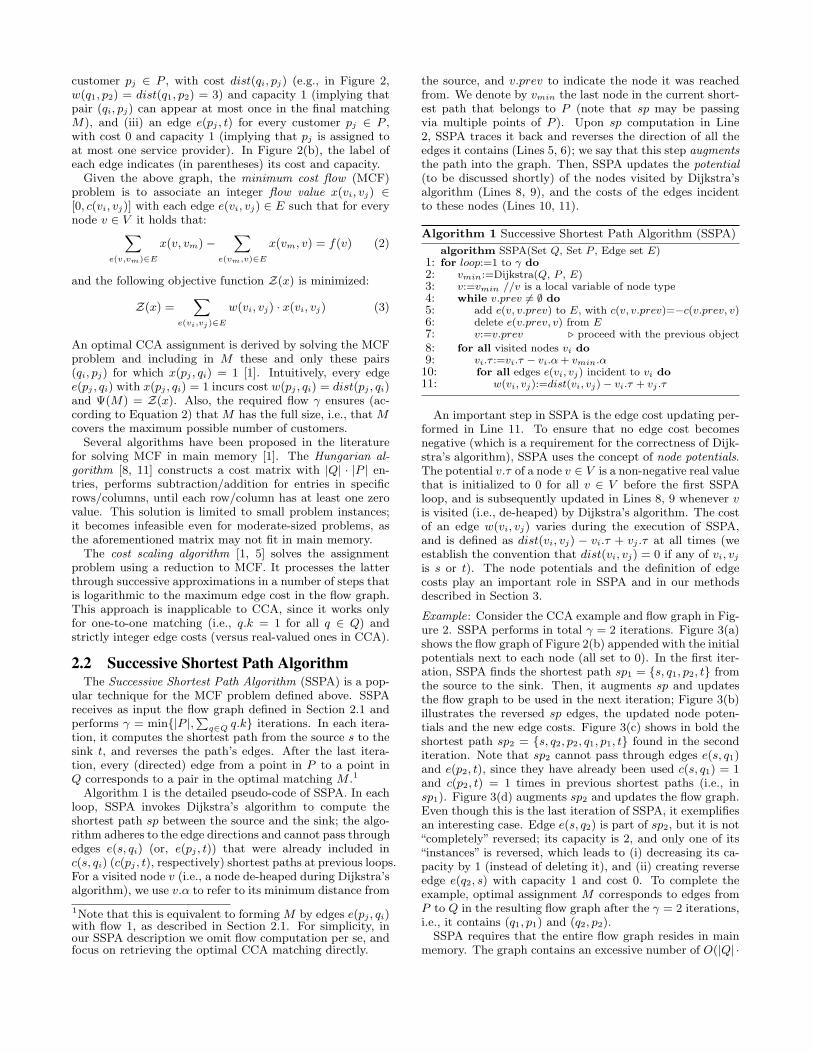
Algorithm 1 is the detailed pseudo-code of SSPA. In eachloop, SSPA invokes Dijkstra’s algorithm to compute theshortest path sp between the source and the sink; the algo-rithm adheres to the edge directions and cannot pass throughedges e(s, qi) (or, e(pj , t)) that were already included inc(s, qi) (c(pj , t), respectively) shortest paths at previous loops.For a visited node v (i.e., a node de-heaped during Dijkstra’salgorithm), we use v.α to refer to its minimum distance from

1Note that this is equivalent to forming M by edges e(pj , qi)with flow 1, as described in Section 2.1. For simplicity, inour SSPA description we omit flow computation per se, andfocus on retrieving the optimal CCA matching directly.

the source, and v.prev to indicate the node it was reachedfrom. We denote by vmin the last node in the current short-est path that belongs to P (note that sp may be passingvia multiple points of P ). Upon sp computation in Line2, SSPA traces it back and reverses the direction of all theedges it contains (Lines 5, 6); we say that this step augmentsthe path into the graph. Then, SSPA updates the potential(to be discussed shortly) of the nodes visited by Dijkstra’salgorithm (Lines 8, 9), and the costs of the edges incidentto these nodes (Lines 10, 11).

Algorithm 1 Successive Shortest Path Algorithm (SSPA)

algorithm SSPA(Set Q, Set P , Edge set E)1: for loop:=1 to γ do2: vmin:=Dijkstra(Q, P , E)3: v:=vmin //v is a local variable of node type4: while v.prev 6= ∅ do5: add e(v, v.prev) to E, with c(v, v.prev)=−c(v.prev, v)6: delete e(v.prev, v) from E7: v:=v.prev . proceed with the previous object

8: for all visited nodes vi do9: vi.τ :=vi.τ − vi.α + vmin.α10: for all edges e(vi, vj) incident to vi do11: w(vi, vj):=dist(vi, vj) − vi.τ + vj .τ

An important step in SSPA is the edge cost updating per-formed in Line 11. To ensure that no edge cost becomesnegative (which is a requirement for the correctness of Dijk-stra’s algorithm), SSPA uses the concept of node potentials.The potential v.τ of a node v ∈ V is a non-negative real valuethat is initialized to 0 for all v ∈ V before the first SSPAloop, and is subsequently updated in Lines 8, 9 whenever vis visited (i.e., de-heaped) by Dijkstra’s algorithm. The costof an edge w(vi, vj) varies during the execution of SSPA,and is defined as dist(vi, vj) − vi.τ + vj .τ at all times (weestablish the convention that dist(vi, vj) = 0 if any of vi, vj

is s or t). The node potentials and the definition of edgecosts play an important role in SSPA and in our methodsdescribed in Section 3.

Example: Consider the CCA example and flow graph in Fig-ure 2. SSPA performs in total γ = 2 iterations. Figure 3(a)shows the flow graph of Figure 2(b) appended with the initialpotentials next to each node (all set to 0). In the first iter-ation, SSPA finds the shortest path sp1 = {s, q1, p2, t} fromthe source to the sink. Then, it augments sp and updatesthe flow graph to be used in the next iteration; Figure 3(b)illustrates the reversed sp edges, the updated node poten-tials and the new edge costs. Figure 3(c) shows in bold theshortest path sp2 = {s, q2, p2, q1, p1, t} found in the seconditeration. Note that sp2 cannot pass through edges e(s, q1)and e(p2, t), since they have already been used c(s, q1) = 1and c(p2, t) = 1 times in previous shortest paths (i.e., insp1). Figure 3(d) augments sp2 and updates the flow graph.Even though this is the last iteration of SSPA, it exemplifiesan interesting case. Edge e(s, q2) is part of sp2, but it is not“completely” reversed; its capacity is 2, and only one of its“instances” is reversed, which leads to (i) decreasing its ca-pacity by 1 (instead of deleting it), and (ii) creating reverseedge e(q2, s) with capacity 1 and cost 0. To complete theexample, optimal assignment M corresponds to edges fromP to Q in the resulting flow graph after the γ = 2 iterations,i.e., it contains (q1, p1) and (q2, p2).

SSPA requires that the entire flow graph resides in mainmemory. The graph contains an excessive number of O(|Q| ·

s

q2

q1 p1

p2

t

(4,1)

(7,1)

(3,1) (10,1)

(0,1)

(0,1)(0,2)

(0,1)

τ = 0

τ = 0 τ = 0

τ = 0τ = 0

τ = 0 s

q2

q1 p1

p2

t

(1,1)

(4,1)

(0,1) (7,1)

(0,1)

(0,1)(0,2)

(0,1)

τ = 3

τ = 3 τ = 0

τ = 0τ = 3

τ = 0

s

q2

q1 p1

p2

t

(1,1)

(4,1)

(0,1) (7,1)

(0,1)

(0,1)(0,2)

(0,1)

τ = 3

τ = 3 τ = 0

τ = 0τ = 3

τ = 0 s

q2

q1 p1

p2

t

(0,1)

(0,1)

(0,1) (2,1)

(0,1)

(0,1)(0,1)

(4,1)

τ = 8

τ = 8 τ = 1

τ = 4

τ = 0(0,1)

τ = 0

s

q2

q1 p1

p2

t

(4,1)

(7,1)

(3,1) (10,1)

(0,1)

(0,1)(0,2)

(0,1)

τ = 0

τ = 0 τ = 0

τ = 0τ = 0

τ = 0 s

q2

q1 p1

p2

t

(1,1)

(4,1)

(0,1) (7,1)

(0,1)

(0,1)(0,2)

(0,1)

τ = 3

τ = 3 τ = 0

τ = 0τ = 3

τ = 0

s

q2

q1 p1

p2

t

(1,1)

(4,1)

(0,1) (7,1)

(0,1)

(0,1)(0,2)

(0,1)

τ = 3

τ = 3 τ = 0

τ = 0τ = 3

τ = 0 s

q2

q1 p1

p2

t

(0,1)

(0,1)

(0,1) (2,1)

(0,1)

(0,1)(0,1)

(4,1)

τ = 8

τ = 8 τ = 1

τ = 4

τ = 0(0,1)

τ = 0

(a) Found sp1 (b) Augmenting sp1

s

q2

q1 p1

p2

t

(4,1)

(7,1)

(3,1) (10,1)

(0,1)

(0,1)(0,2)

(0,1)

τ = 0

τ = 0 τ = 0

τ = 0τ = 0

τ = 0 s

q2

q1 p1

p2

t

(1,1)

(4,1)

(0,1) (7,1)

(0,1)

(0,1)(0,2)

(0,1)

τ = 3

τ = 3 τ = 0

τ = 0τ = 3

τ = 0

s

q2

q1 p1

p2

t

(1,1)

(4,1)

(0,1) (7,1)

(0,1)

(0,1)(0,2)

(0,1)

τ = 3

τ = 3 τ = 0

τ = 0τ = 3

τ = 0 s

q2

q1 p1

p2

t

(0,1)

(0,1)

(0,1) (2,1)

(0,1)

(0,1)(0,1)

(4,1)

τ = 8

τ = 8 τ = 1

τ = 4

τ = 0(0,1)

τ = 0

s

q2

q1 p1

p2

t

(4,1)

(7,1)

(3,1) (10,1)

(0,1)

(0,1)(0,2)

(0,1)

τ = 0

τ = 0 τ = 0

τ = 0τ = 0

τ = 0 s

q2

q1 p1

p2

t

(1,1)

(4,1)

(0,1) (7,1)

(0,1)

(0,1)(0,2)

(0,1)

τ = 3

τ = 3 τ = 0

τ = 0τ = 3

τ = 0

s

q2

q1 p1

p2

t

(1,1)

(4,1)

(0,1) (7,1)

(0,1)

(0,1)(0,2)

(0,1)

τ = 3

τ = 3 τ = 0

τ = 0τ = 3

τ = 0 s

q2

q1 p1

p2

t

(0,1)

(0,1)

(0,1) (2,1)

(0,1)

(0,1)(0,1)

(4,1)

τ = 8

τ = 8 τ = 1

τ = 4

τ = 0(0,1)

τ = 0

(c) Found sp2 (d) Augmenting sp2

Figure 3: Example of SSPA

|P |) edges, which do not fit in memory for large probleminstances. Moreover, the time complexity of SSPA is O(γ ·(|E| + |V | · log|V |)), where O(|E| + |V | · log|V |) is the costto compute a shortest path. Since in our targeted applica-tions |E| is quite large (O(|P | · |Q|)), SSPA is particularlyslow. Another fundamental problem of SSPA is that it isdesigned for main memory processing and ignores the I/Ocost, which generally is the most critical performance factorin the processing of disk-resident data.

2.3 Spatial QueriesPoint sets are usually indexed by spatial access methods

in order to accelerate query processing. The R-tree [6] andits variants (e.g., [9, 2]) are the most common such indexes.The R-tree is a disk-based, balanced tree that groups to-gether nearby points into leaf nodes, and recursively groupsthese leaf nodes into higher level nodes (again based on theirproximity) up to a single root. Each non-leaf entry is as-sociated with a minimum bounding rectangle (MBR) thatencloses all the points in the subtree pointed by it.

Typical spatial search operations on a point set P arerange and nearest neighbor (NN) queries. Given a rangevalue r and a query point q, the r-range query retrieves allpoints of P within (Euclidean) distance r from q. If P isindexed by an R-tree, this query is evaluated by followingrecursively R-tree entries that intersect the circular disk withcenter at q and radius r. The K-nearest neighbor (KNN)query receives as input an integer K and a query point q, andreturns the K points of P that are closest to q. The state-of-the-art KNN processing technique is the best-first NNalgorithm [7], which employs a heap for organizing encoun-tered R-tree entries and visiting them in ascending order oftheir distance from q, until K points are discovered.

Assignment problems in large spatial databases have re-cently received considerable attention. Specifically, [12, 14]study the spatial matching (SM) join. Given two point setsP and Q, the SM join iteratively outputs the closest pair[4] (p, q) in P × Q, reports (p, q) as an assigned pair, andremoves both p and q from their corresponding datasets be-fore the next iteration. This procedure continues until eitherP or Q becomes empty. [14] enhances the performance ofa naıve (i.e., repetitive closest pair) algorithm with severalgeometric observations. SM is related, yet different by def-inition from CCA; SM greedily performs local assignmentsinstead of minimizing the global assignment cost.

3. EXACT METHODSIn this section we present our methods for computing op-

timal CCA assignments. In accordance with most real-worldscenarios, we consider that Q (the set of of service providers)is much smaller than P (the set of customers). We assumethat Q fits into main memory, while P is stored on the disk.In the following we consider two-dimensional points and thatP is indexed by an R-tree. However, our algorithms can eas-ily extend to problems of higher dimensionality and otherspatial access methods.

As explained in Section 2.2, SSPA is not applicable tolarge CCA problem instances, as its (complete bipartite)flow graph leads to excessive memory consumption and ex-pensive shortest path computations. To alleviate the spaceand running time problems incurred by the huge flow graph,we develop incremental SSPA-based algorithms that startfrom an empty flow graph and insert edges into it gradually.Intuitively, edges with low edge weights are highly probableto indicate pairs in the optimal assignment. A fundamen-tal theorem (presented below) formalizes this intuition andexcludes from consideration edges whose cost is too high toaffect the result of SSPA. Additionally, our techniques ex-ploit the spatial index of P to further improve performance.

Our general idea is to perform the search in a subgraphwith edge set Esub ⊆ E, where E is the complete set of flowgraph edges. We refer to the Euclidean distance betweenthe nodes of an edge as its length. Let function φ(·) take asinput a set of edges and return the minimum edge lengthin it. To facilitate the derivation of distance bounds, werequire Esub to be distance-bounded, as defined below.

Definition 1. An edge set Esub ⊆ E is said to be distance-bounded if

∀ e(qi, pj) ∈ Esub, dist(qi, pj) ≤ φ(E − Esub)

In other words a distance-bounded Esub contains thoseand only those edges in E that have length less than orequal to a threshold (i.e., φ(E − Esub)). Conversely, all theremaining edges (i.e., edges in E−Esub) have length greaterthan or equal to that threshold. We stress that function φ(·)and Definition 1 refer to edge lengths, and not to their costs(note that costs vary during the execution of our algorithmsbecause the node potentials are updated).

Suppose that we are given a distance-bounded edge setEsub. Consider an execution of Dijkstra’s algorithm on Esub

that computes the shortest path sp between the source andthe sink, and the potential values vi.τ for every node vi,derived as described in Section 2.2. The following theoremdetermines the condition that should hold so that sp is theshortest path on the complete edge set E.

Theorem 1. Consider a distance-bounded edge set Esub ⊆E. Let sp be the shortest path (between source and sink) inEsub and τmax = max {vi.τ |vi ∈ V } be the maximum poten-tial value. If the total cost of sp is at most φ(E − Esub) −τmax, then sp is also the shortest path (between source andsink) on the complete flow graph.

Proof. Consider the edges in E−Esub. First, their min-imum length is φ(E−Esub). Second, as explained in Section2.2, their costs are defined as w(vi, vj) = dist(vi, vj)−vi.τ +vj .τ . Since dist(vi, vj) ≥ φ(E − Esub), vi.τ ≤ τmax, andvj .τ ≥ 0, it holds that

w(vi, vj) ≥ φ(E − Esub)− τmax,∀e(ci, vj) ∈ E − Esub

According to the above (and since edge costs are always non-negative), any path passing through an edge in E − Esub

has at least a cost of φ(E − Esub)− τmax. Therefore, if theshortest path sp (on Esub) has total cost no greater thanφ(E−Esub)−τmax, then it must be the shortest path in theentire E too.

In the following we investigate approaches for graduallyexpanding the subgraph Esub and use it to derive CCA pairs.Our first solution incrementally enlarges range searches aroundpoints in Q. The other two aim at further reducing the sizeof Esub by replacing range queries with incremental nearestneighbor searches [7].

3.1 Range Incremental AlgorithmOur first method is the Range Incremental Algorithm (RIA).

Algorithm 2 presents the pseudo-code of RIA. The procedurestarts with an initial range T equal to a system parameterθ. For every point qi ∈ Q, RIA performs a T -range search inP ; for each retrieved point pj ∈ P , edge e(qi, pj) is insertedinto Esub. RIA invokes SSPA in the resulting Esub.

Observe that T serves as a lower bound for φ(E − Esub)(i.e., φ(E−Esub) ≥ T ). Assume that a Dijkstra execution inLine 6 finds a shortest path sp. If the total cost of sp is lessthan T−τmax (Line 7)2, then it is also less than φ(E−Esub)−τmax. In this case, sp is valid according to Theorem 1; i.e., itis a shortest path in the entire E too. Thus, we augment sp,updating potential values and sp edges in the graph (Lines8-10) as in the basic SSPA technique. Otherwise (i.e., spcost is higher than T − τmax), the sp is not valid and isnot augmented; RIA performs new range searches with anextended T in order to insert more edges into Esub (Lines 12-15). Specifically, we extend T by θ and execute an annularrange search for each point qi ∈ Q, so that points of Pwithin the distance range (T − θ, T ] from qi are identified(and the corresponding edges are inserted into Esub). Then,RIA resumes from the iteration it stopped. RIA continuesthis way and terminates when γ = min{|P |,

∑q∈Q q.k} valid

shortest paths are found in total. It can be easily shownthat the RIA matching is identical to that of SSPA, whichconsiders the entire E.

Algorithm 2 Range Incremental Algorithm (RIA)

algorithm RIA(Set Q, Set P , Value θ)1: T :=θ; τmax:=0; Esub:=∅2: for all qi ∈ Q do3: P ′:=Range-Search(qi,T )4: insert edge e(qi, pj) into Esub, for each pj ∈ P ′

5: for loop:=1 to γ do6: vmin:=Dijkstra(Q, P , Esub)7: if vmin.α ≤ T − τmax then8: v:=ReverseEdges()9: UpdatePotentials()10: τmax:=max {qi.τ |qi ∈ Q} . the highest potential11: else12: loop--; T :=T + θ13: for all qi ∈ Q do14: P ′:=Annular-Range-Search(qi,T − θ,T )15: insert edge e(qi, pj) into Esub, for each pj ∈ P ′

2To clarify the condition in Line 7, the total cost of sp is bydefinition equal to vmin.α, since c(vmin, t) is always 0.

3.2 Nearest Neighbor Incremental AlgorithmRIA constrains the search on a small edge set Esub by us-

ing system parameter θ. However, it is hard to fine-tune θ orderive it analytically. When θ is too large, set Esub grows,leading to long computation time. In case θ is too small,RIA performs numerous range searches, incurring high I/Ocost. To tackle this problem, we develop a Nearest NeighborIncremental Algorithm (NIA), which performs incrementalnearest neighbor search [7] to expand edge set Esub. Al-gorithm 3 is the pseudo-code of NIA. We use a min-heapH, that organizes encountered edges in ascending cost or-der. Specifically, we first compute for each point qi ∈ Q itsnearest neighbor pj in P and insert the corresponding edgee(qi, pj) into H. In each loop, NIA de-heaps the shortestedge e(qi, pj) from H and inserts it into Esub (Lines 7, 8).Then, it computes the next nearest neighbor of qi and in-serts the corresponding edge into H (Lines 9, 10). Next, itcomputes the shortest path sp in the new Esub.

Due to the min-heap ascending ordering and the incre-mental nearest neighbor search, it is guaranteed that the topedge in H has the minimum weight of edges in E − Esub.Letting TopKey(H) be the key (i.e., length) of the top entryin H, it holds that (i) Esub is a distance-bounded edge setand (ii) φ(E − Esub) = TopKey(H). From Theorem 1 itfollows that if the cost of sp (i.e., vmin.α) is no greater thanTopKey(H) − τmax, then sp is a valid shortest path and isthus augmented into the graph.

Otherwise (i.e., if the sp cost is larger than TopKey(H)−τmax), sp is invalid and ignored. In this case, NIA de-heapsthe top edge e(qi, pj) from H and inserts it into Esub. Forthe qi node of the de-heaped edge, NIA finds its next nearestneighbor in P . Letting pm be this neighbor, edge e(qi, pm)is inserted into H (with key equal to its length). A newshortest path is computed in the expanded Esub and theprocedure is repeated; the current iteration is consideredcomplete when a valid shortest path is computed and aug-mented into the graph. Overall, NIA terminates after γcompleted iterations (equivalently, after augmenting γ validshortest paths).

Algorithm 3 Nearest Neighbor Incremental Algo. (NIA)

algorithm NIA(Set Q, Set P )1: H:=new min-heap2: τmax:=0; Esub:=∅3: for all qi ∈ Q do4: pj :=NN of qi in P5: insert 〈e(qi, pj), dist(qi, pj)〉 into H

6: for loop:=1 to γ do7: de-heap the top entry 〈e(qi, pj), dist(qi, pj)〉 from H8: insert edge e(qi, pj) into Esub

9: pm:=next NN of qi in P10: insert 〈e(qi, pm), dist(qi, pm)〉 into H11: vmin:=Dijkstra(Q, P , Esub)12: if vmin.α ≤ TopKey(H) − τmax then13: v:=ReverseEdges()14: UpdatePotentials()15: τmax:=max {qi.τ |qi ∈ Q} . the highest potential16: else17: loop-- . Invalid path; go to Line 7

3.3 Incremental On-demand AlgorithmIn this section, we present the Incremental On-demand

Algorithm (IDA), which improves on NIA by pruning more

edges and accelerating sp computations. IDA is based onthe concept of full service providers and full customers.

Definition 2. A service provider qi ∈ Q is said to befull when edge e(s, qi) has already been used qi.k times inprevious (valid) shortest paths.

For a full qi, since e(s, qi) (with a fixed cost 0) has reachedits capacity, Dijkstra’s algorithm can no longer pass throughthis edge. In other words, the shortest path from s to qi canno longer be this edge and, thus, qi.α (i.e., the minimum costfrom s to qi) may be greater than 0. This fact is exploitedby IDA, which leads to a more effective pruning of edgesincident to qi.

IDA uses an edge heap H just like NIA. Unlike NIA, wherethe key of the edges in H is their length dist(qi, pm), in IDAthe key of an edge e(qi, pm) is qi.α+dist(qi, pm). The ratio-nale is that if qi is full, any sp going through qi should havecost at least qi.α + dist(qi, pm). This leads to earlier termi-nation and smaller Esub, since edges reachable through fullservice providers are not de-heaped (and, thus, not insertedinto Esub) unnecessarily early.

As qi.α varies, whenever some Dijkstra execution visits afull qi ∈ Q and updates qi.α to a new value, IDA accordinglyupdates the key of its corresponding edge e(qi, pj) in H tothe new qi.α+dist(qi, pj). Note that (in both NIA and IDA)for every qi ∈ Q there is exactly one edge in H from qi tosome pj ∈ P at all times. It is easy to show the correctness ofIDA, after replacing φ(E−Esub) by Φ(E−Esub) in Theorem1. Φ(E − Esub) models the minimum possible cost an spcould have if it passed through some edge in E − Esub.

Similar to full service providers, IDA also exploits theproperties of full customers to improve the running timeand, specifically, to accelerate shortest path computations.Below we formally define full customers and provide a the-orem that allows sp retrieval without invoking Dijkstra’salgorithm.

Definition 3. A customer pj ∈ P is said to be full whenedge e(pj , t) has already been used in a previous (valid) short-est path.

Theorem 2. If no q ∈ Q is full, then the shortest path(between source s and sink t) passes through a single edgee(qi, pj); i.e., sp = {e(s, qi), e(qi, pj), e(pj , t)}, where qi ∈ Q,pj ∈ P . Furthermore, e(qi, pj) is the shortest edge in Esub

with a non-full pj.

Proof. Since no q ∈ Q is full, all q ∈ Q are inserted intothe Dijkstra heap and visited (with cost q.α = 0) beforeany p ∈ P . Therefore, after de-heaping the first pj ∈ P ,and if pj is full, Dijkstra cannot return to any q ∈ Q. As aresult, the current sp must be passing through exactly oneedge e(qi, pj) (with a non-full pj) followed by e(pj , t), i.e.,sp = {e(s, qi), e(qi, pj), e(pj , t)}. Since qi and pj are non-full,w(s, qi) = w(pj , t) = 0 and the sp cost is w(qi, pj).

It remains to show that the cost order among edges e(q, p) ∈Esub with non-full p coincides with their length order. Asdescribed in Section 2.2, w(q, p) = dist(q, p)−q.τ +p.τ . Notethat a node p ∈ P becomes full when Dijkstra’s algorithmvisits it for the first time. Equivalently, all non-full oneshave never been visited by Dijkstra’s algorithm and theirpotentials remain 0 since the initialization of the problem.As a result, p.τ = 0, and w(q, p) = dist(q, p)−q.τ . Also, thefact that all q ∈ Q are non-full leads to their potentials being

updated in every IDA iteration to the same exact value (inLine 9 in Algorithm 1). Thus, the cost order among edgeswith non-full p coincides with their distance order.

According to the above theorem, as long as no serviceprovider q ∈ Q is full, IDA computes the current sp, with-out invoking Dijkstra’s algorithm, by iteratively de-heapingedges e(qi, pj) from H3. If pj is full, we directly insert itinto Esub and de-heap the next entry; otherwise we reportsp = {e(s, qi), e(qi, pj), e(pj , t)}. Note that after de-heapingany edge e(qi, pj) from H, we en-heap the edge from qi toits next nearest customer (as in Lines 7-10 of Algorithm 3).

Algorithm 4 is the pseudo-code of IDA. Lines 1-5 initializeEsub identically to NIA. At Line 9 we compute the currentsp. Note that if no service provider is full, we derive spusing Theorem 2 and the method described above (we omitthis enhancement from the pseudo-code for readability). AtLines 10-12, if the last sp computation visited some full q ∈Q and altered its q.α value, then we accordingly updatethe key of its corresponding edge e(q, p) in H to the newq.α + dist(q, p) (Line 12). Lines 13-14 retrieve the next NNof qi (qi refers to e(qi, pj) de-heaped at Line 7) and insert thecorresponding edge into H. Note that we perform this afterupdating the q.α values at Lines 10-12 so that the en-heapededge has an up-to-date key.

Algorithm 4 Incremental On-demand Algorithm (IDA)

algorithm IDA(Set Q, Set P )1: H:=new min-heap2: τmax:=0; Esub:=∅3: for all qi ∈ Q do4: pj :=first NN of qi in P5: insert 〈e(qi, pj), dist(qi, pj)〉 into H

6: for loop:=1 to γ do7: de-heap 〈e(qi, pj), key〉 from H8: insert e(qi, pj) into Esub

9: vmin:=Dijkstra(Q, P, Esub)10: for all visited q ∈ Q do11: if q is full and q.α changed in Line 9 then12: update q.α in H

13: pm:=next NN of qi in P14: insert 〈e(qi, pm), qi.α + dist(qi, pm)〉 into H15: if vmin.α ≤ TopKey(H) − τmax then16: v:=ReverseEdges()17: UpdatePotentials()18: τmax:=max {qi.τ |qi ∈ Q} . the highest potential19: else20: loop-- . Invalid path; go to Line 7

Example: Consider the example in Figure 4(a), where thetable at the top illustrates the lengths of all encounterededges (i.e., edges in Esub and in the heap). The flow graphshown skips the source and sink for clarity and includes onlyedges between service providers and customers. Service pro-vider q1 (shown shaded) is full with q1.α = 3. Dashed edgese(q1, p3), e(q2, p5) and the bold one e(q3, p4) have been en-heaped but not yet inserted into Esub. At the bottom, H1

and H2 illustrate the heap contents in NIA and IDA, re-spectively, assuming that so far they proceeded identically.Their difference is the key of e(q1, p3), which is 7 in NIAand 10 in IDA (since dist(q1, p3) = 7 and q1.α = 3). Thisleads to a different insertion order into Esub and a faster IDA

3While no q is full, all keys in H are equal to the correspond-ing edge lengths.

termination. For the current sp to be valid, in Line 12 ofAlgorithm 3 (in Line 15 of Algorithm 4), NIA (IDA) requiresthat its cost is no greater than 7-τmax (8-τmax), where 7 (8)is the TopKey(H1) value (TopKey(H2), respectively). Thisimplies that the current IDA iteration has higher chances toterminate without needing to insert new edges and re-invokeDijkstra’s algorithm.

<q1 p3, 7> <q3 p4, 8> <q2 p3, 9>H1

H2 <q3 p4, 8> <q2 p3, 9> <q1 p3, 10>

q1

p1

q2

p2

q3

p3

p4

α = 3

α = 0

α = 0

α = ∞

α = 1

α = 1

α = ∞

H2<q2 p3, 9> <q1 p3, 12> <q3 p1, 12>

q1

p1

q2

p2

q3

p3

p4

-84610q3

-

-

p4

9---q2

-715q1

p5p3p2p1dist(qi,pj)

…

…

…

αααα = 5

α = 0

αααα = 2

p5 α = ∞

…

p5

α = ∞

αααα = 3

α = 1

αααα = 2

α = ∞

<q1 p3, 7> <q3 p4, 8> <q2 p5, 9>H1

H2 <q3 p4, 8> <q2 p5, 9> <q1 p3, 10>

q1

p1

q2

p2

q3

p3

p4

α = 3

α = 0

α = 0

α = 1

α = 1

H2 <q2 p5, 9> <q1 p3, 12> <q3 p1, 12>

q1

p1

q2

p2

q3

p3

p4

-84610q3

--

p4

9---q2

-715q1

p5p3p2p1dist(qi,pj)

…

…

…

α = 5

α = 0

α = 2

p5

…

p5

α = 3

α = 1

α = 2

<q1 p3, 7> <q3 p4, 8> <q2 p5, 9>H1

H2 <q3 p4, 8> <q2 p5, 9> <q1 p3, 10>

q1

p1

q2

p2

q3

p3

p4

α = 3

α = 0

α = 0

α = 1

α = 1

H2 <q2 p5, 9> <q1 p3, 12> <q3 p1, 12>

q1

p1

q2

p2

q3

p3

p4

-84610q3

--

p4

9---q2

-715q1

p5p3p2p1dist(qi,pj)

…

…

…

α = 5

α = 0

α = 2

p5

…

p5

α = 3

α = 1

α = 2

(a) IDA versus NIA (b) Key update

Figure 4: Utilizing full service providers in IDA

Let us now focus on IDA. Since the top edge in H2 ise(q3, p4) (shown bold), we insert it into Esub. Figure 4(b)shows the new flow graph, assuming that the subsequentDijkstra execution returned an sp passing through e(q3, p4).Assuming that q3.k = 2, augmenting this sp makes q3 fullwith q3.α = 2, and alters q1.α to 5. Since q1.α has changed,IDA updates the key of e(q1, p3) in H2 to dist(q1, p3)+qi.α =12. Then, we find the next NN of q3 (i.e., p1) and insertthe corresponding edge e(q3, p1) into H2 with key q3.α +dist(q3, p1) = 12. The bold edge (i.e., e(q2, p5)) is the oneto be inserted next into Esub.

3.4 OptimizationsIn this section we describe two enhancements that apply

to NIA and IDA. Section 3.4.1 proposes a technique thataccelerates Dijkstra’s algorithm by reusing its previous com-putations. Section 3.4.2 presents an incremental all nearestneighbor (ANN) search that reduces the I/O cost.

3.4.1 Reducing Dijkstra ExecutionsUnlike the bulk discovery and insertion of edges (through

range search) in RIA, NIA/IDA apply incremental NN searchto discover the edges one-by-one, keeping Esub small. How-ever, since Esub expands slowly, NIA/IDA may perform nu-merous Dijkstra executions. To accelerate processing, we re-duce the cost of Dijkstra executions in NIA/IDA by reusing(i) the vi.α values computed in the previous sp computationand (ii) utilizing the entries that remained inside the Di-jkstra heap upon termination. Assume that in the currentNIA/IDA iteration some (invalid) sp has been computed,and that we need to find a new sp after inserting a new edgee(q, p) into Esub (in Line 8 of Algorithm 3 or Algorithm 4,respectively). Let Hd be the Dijkstra search heap after lastsp computation.

Our objective is (i) to identify the visited nodes v whosev.α value is affected by e(q, p) (i.e., e(q, p) leads to a short-est path from the sink to v) and, eventually, (ii) to updatethe keys of nodes inside Hd. This is performed by the PathUpdate Algorithm (PUA) to be described shortly. Upon ter-mination of PUA, a new Dijkstra execution is performed,which however directly uses the updated Hd and avoids vis-iting nodes de-heaped in previous sp computation(s) in thecurrent NIA/IDA iteration.

PUA initializes an empty min-heap Hf to play the role ofa Dijkstra-like search heap among previously visited nodes.Hf organizes its entries (nodes) in ascending order of theirα values. First, we insert into Hf the q node of the newedge e(q, p). Next, we iteratively de-heap the top node vi

from Hf and examine whether nodes vj connected to vi canbe reached through a shortest path via vi. In particular, ifvj .α > vi.α+w(vi, vj) then vj .α is updated to vi.α+w(vi, vj)and vj .prev is set to vi (to indicate that vj is now reachablevia vi). If vj is in Hd or Hf , its key is updated to vj .α in itscontaining heap. Otherwise (i.e., if vj is neither in Hd norHf ), it is inserted into Hf with key vj .α. PUA terminateswhen Hf becomes empty. Algorithm 5 presents PUA.

Algorithm 5 Path Update Algorithm (PUA)

algorithm PUA(Set Q, Set P , Heap Hd, Edge set Esub, Edgee(q, p))

1: Hf :=new min-heap2: insert 〈q, q.α〉 into Hf

3: while Hf is not empty do4: de-heap top node vi (with the lowest vi.α value) from Hf

5: for all edges e(vi, vj) ∈ Esub outgoing from vi do6: if vj .α > vi.α + w(vi, vj) then7: vj .α:=vi.α + w(u, v); vj .prev:=vi

8: if vj ∈ Hd then9: update vj .α in Hd

10: else if vj ∈ Hf then11: update vj .α in Hf

12: else13: insert 〈vj , vj .α〉 into Hf

Example: We illustrate the PUA technique with an exam-ple. Figure 5(a) shows the current Esub edges between (somenodes of) sets Q and P , the α values of these nodes, and theedge costs (numbers above each edge) after the last Dijkstraexecution. The visited nodes are illustrated shaded, whilethe nodes remaining in Hd are q4 and p3 (having bold bor-ders and lighter gray color). Consider that edge e(q1, p2)with cost w(q1, p2) = 2 is inserted into Esub. Figure 5(b)shows the new edge (in bold) and the PUA steps. First,q1 is inserted into Hf with key q1.α = 0. Its de-heapingleads to adjacent node p2 which is reachable with a lowercost (than the current p2.α) via q1. Thus, p2 is inserted intoHf with key equal to the new p2.α = q1.α + w(q1, p2) = 2.Similarly, the de-heaping of p2 leads to updating the key ofq4 in Hd to the new q4.α = 3. After these changes, the newsp can be computed by directly using Hd = {〈q4, 3〉, 〈p3, 5〉}in the new Dijkstra execution. Note that the shortest pathsto (and, accordingly, the α values of) q2, q3, p1, p3 have notbeen affected by the insertion of e(q1, p2) and the new spcomputation avoids unnecessary costs for them.

PUA can utilize results only among Dijkstra executionstaking place as part of the same NIA/IDA iteration. Thereason why reusing cannot span multiple iterations is thatsp augmentation (which signals the end of an iteration) al-

q1 p1

q2 p2

q3 p3

p4

α = 1

α = 3

α = 5

… …

q4

α = 0

α = 1

α = 0

α = 4

q1

p2

p4

α = 2

… …

q4

α = 0

α = 3

2

1

2

10

2

15

2

(a) Previous state

q1 p1

q2 p2

q3 p3

p4

α = 1

α = 3

α = 5

… …

q4

α = 0

α = 1

α = 0

α = 4

q1

p2

p4

α = 2

… …

q4

α = 0

α = 3

2

1

2

10

2

15

2

(b) Insertion of e(q1, p2)

Figure 5: Example of PUA

ters many edges, by reversing their directions and modifyingtheir costs. Another important remark is that IDA uses theabove PUA-based optimization only after some of the ser-vice providers become full, because until then shortest pathsare computed using Theorem 2 directly.

3.4.2 Incremental ANN ProcessingOur CCA algorithms invoke numerous NN search oper-

ations around the service providers to the R-tree RP thatindexes the customers P . To reduce the I/O cost, we em-ploy an incremental all-nearest-neighbors technique. First,we form service provider groups Gm based on their Hilbertspace-filling curve ordering. For each group Gm we maintaina min-heap Hm that organizes encountered R-tree entries ein ascending mindist(MBR(Gm), MBR(e)) order. For ev-ery qi ∈ Gm we maintain a candidate min-heap resi thatorders all encountered customers (i.e., candidate NNs) inascending distance from qi.

When we need to compute the (next) NN of some qi ∈Gm, we iteratively de-heap and visit the top R-tree en-try in Hm. If the de-heaped entry is a point p ∈ P , weinsert it into the candidate min-heap of every service pro-vider in Gm. The procedure terminates when the top can-didate pj in resi has key smaller than or equal to the topentry in Hm; i.e., dist(qi, pj) is smaller than or equal tomindist(MBR(Gm), MBR(e)) for every unvisited R-tree en-try e. At that point, we de-heap pj from resi and report itas the (next) NN of qi. Algorithm 6 is a pseudo-code for theabove procedure.

Algorithm 6 Incremental ANN Search

algorithm ANN(Group Gm, R-tree RP , Service provider qi)1: while top entry in resi has key > key of top entry in Gm do2: de-heap top entry e from Hm

3: if e is an directory entry of R-tree RP then4: visit node pointed by e and insert its entries into Hm

5: else . E is a leaf level entry, i.e., a point p ∈ P6: for all qk in Gm do7: insert 〈p, dist(p, qk)〉 into resk

8: de-heap top entry 〈pj , dist(pj , qi)〉 from resi

9: return pj as the next NN of qi

4. APPROXIMATE METHODSTime-critical applications may favor fast answers over ex-

act ones. This motivates us to develop approximate CCAsolutions. In this section, we propose a methodology thatprovides a tunable trade-off between result accuracy and re-sponse time, and comes with theoretical guarantees for theassignment cost.

Our general approach consists of three phases. The firstone is the partitioning phase, in which we form groups Gm

of either the points in Q or points in P , so that the diagonalof their MBR does not exceed a threshold δ. Parameter δ isused to control the quality of the assignment; the smaller δis the better the computed matching approximates the opti-mal. The second phase, called concise matching, solves op-timally a small CCA problem extracting one representativepoint per group Gm and using the set of representatives asthe set of service providers (customers). Finally, the refine-ment phase uses the assignment produced in the previousstep to derive a matching on the entire sets P and Q.

Sections 4.1 and 4.2 describe two methods, called Ser-vice Provider Approximation (SA) and Customer Approx-imation (CA). SA and CA follow different approaches forpartitioning and subsequent concise matching. Specifically,SA groups the service providers and solves concise match-ing in the entire P , while CA groups the customers andperforms concise matching in the entire Q.4 Section 4.3 de-scribes refinement techniques that could be used with eitherSA or CA. Finally, Section 4.4 provides error bounds forboth approaches.

4.1 Service Provider ApproximationPartitioning in SA is performed on set Q. The points q ∈

Q are sorted according to their Hilbert values and processedin this order. We start with zero service provider groups.Each point q, in turn, is inserted into an existing group Gm

so that the diagonal of Gm’s MBR does not exceed δ. If nosuch group is found, then a new group is formed to includeq. The process is repeated until all service providers q ∈ Qare grouped.

We proceed to concise matching by extracting one repre-sentative point per group. The representative point gm ofa group Gm has capacity gm.k =

∑q∈Gm

q.k and is locatedat its geometric centroid ; each coordinate of gm is equal tothe weighted average of points inside Gm. Weighting is per-formed according to the capacities q.k of points q ∈ Gm, e.g.,the x-coordinate gm.x of gm is 1∑

q∈Gmq.k

∑q∈Gm

(q.x · q.k).

Figure 6 shows a scenario where Q = {q1, ..., q10}. As-sume that SPP produces the illustrated groups G1, G2, G3

according to parameter δ. The dashed lines correspond togroup MBR diagonals and their lengths cannot be longerthan δ. The representatives of these groups are shown asgray points g1, g2 and g3. Assuming that all q ∈ Q havecapacity q.k = 2, then the representative capacities areg1.k = 6, g2.k = 6, g3.k = 8.

q8q4q1 q10

q6q3

q7q5q2

q9g1–g2–

g3–G1G3

G2

Figure 6: Service provider partitioning

4We note here that we attempted to combine SA and CA(i.e., to group both Q and P ), but this led to a very poormatching. Thus, we omit this hybrid method.

The resulting representatives form set Q′ which is used asan approximation of Q. The concise matching of SA solvesan exact CCA problem over Q′ and P . This step is per-formed by the IDA algorithm described in Section 3.3, be-cause (as will be demonstrated by our experiments) it is themost efficient among the exact methods. The matching M ′

produced by this step will be refined into the final matchingM using one of the techniques presented in Section 4.3.

4.2 Customer ApproximationCA is similar to SA, but groups customers instead of ser-

vice providers. Recall that P is indexed by an R-tree. Wefirst initialize a set S of customer groups to ∅. Given pa-rameter δ, we traverse the R-tree. Starting from the rootentries, we compare the MBR diagonal of each of them withδ. If the diagonal of entry e is smaller than or equal to δ,we insert it into S (the corresponding group of customersare those in the subtree rooted at e). Otherwise (i.e., e’sdiagonal is larger than δ), we visit the corresponding nodeand recursively repeat this procedure for its entries.

R-tree leaves are an exception to this procedure. In par-ticular, if δ is small, it is possible that we reach an entrye corresponding to an R-tree leaf whose diagonal is largerthan δ. An option would be to insert into S all points in e,but this would result in a large S. Thus, we handle e as fol-lows. We conceptually split its MBR into two equal halveson its longest dimension. We repeat this process until thediagonal of each partition becomes smaller than or equal toδ. Then, we insert the resulting conceptual entries into S.

Upon termination of the above procedure, all entries inS have diagonal smaller than δ and the union of points intheir subtrees is the entire P . The size of S, however, can bereduced (without violating the δ constraint) by an extra stepthat merges its contents. Specifically, we use a proceduresimilar to SA and group entries in S into conceptual hyper-entries whose diagonal does not exceed δ.

Let S be the final set of entries (conceptual or not). Weproduce a set P ′ of customer representatives as follows. Foreach e ∈ S we derive a representative point g located at thegeometric centroid of e. The representative has weight g.wequal to the number of points in the subtree of e.

To exemplify CA partitioning, assume that the R-tree ofP and parameter δ are as shown in Figure 7 (the R-tree isillustrated both in the spatial domain and as stored on thedisk). We first access the root, and consider its entries e1

and e2. Entry e2 has smaller diagonal than δ and is insertedinto S. This is not the case for e1, whose pointed entries areloaded from the disk. Among e1’s entries, e4 and e5 satisfythe diagonal condition and are included in S. On the otherhand, e3 is a leaf and still has diagonal larger than δ. Thus,we conceptually divide it into two new entries on its longdimension (i.e., x dimension). The resulting e3,1 and e3,2

have small enough diagonal and are placed into S. Entriesinserted into S are shown shaded. In the last step, we mergeentries into larger ones (while still satisfying the δ condition);e4 and e5 form a hyper-entry whose boundaries are showndashed. Every entry in the final S implicitly defines a groupof customers Gm. Set P ′ contains the representatives of thefinal entries in S, i.e., P ′ = {g1, g2, g3, g4}.

In the concise matching phase, CA computes the optimalmatching M ′ between P ′ and Q. This is performed in mainmemory (where P ′ and Q reside) using IDA. Note that inthis setting points in P ′ also have capacities (the represen-

g2–

e1

e2

e3

e5e4

e3,1 e3,2

e6

e7

g4–

g1–

R-tree root

e1

e1 e2

e2

e6 e7e3 e4 e5

δ

g3–

Figure 7: Customer partitioning

tative weights). This is not a problem, since IDA (as wellas RIA and NIA) can handle capacities in the customer sideof the flow graph too. The difference is that M ′ may assign“instances” of a representative to multiple service providers.

4.3 Refinement PhaseIn both SA and CA, we are given a matching M ′ between

one approximate set (i.e., Q′ or P ′) and one original set (Por Q, respectively). In either case, M ′ specifies for eachgroup Gm of service providers (customers) which customers(instances of service providers) are assigned to it. In otherwords, in both SA and CA the refinement phase has to solveseveral smaller problems of assigning a set of customers P ′′

to a set of service providers Q′′ (where the number of pointsp ∈ P ′′ to be assigned to each q ∈ Q′′ is given by the con-cise matching phase). We could run an exact algorithm foreach of these smaller problems. This, however, is expensive.Instead, we propose the following two heuristics5, receivingsmalls sets P ′′ and Q′′ as input.

NN-based refinement : This approach computes the (next)NN of each q ∈ Q′′ in a round-robin fashion in set P ′′.When discovering the NN p of service provider q, we includepair (q, p) in the final assignment M and remove p from P ′′.If q has reached its number of instances to be assigned toP ′′, we also delete q from Q′′.

Exclusive NN refinement : According to this strategy, weidentify the p ∈ P ′′ with the minimum distance from anyq ∈ Q′′ that has not reached its number of instances tobe assigned to P ′′ (according to M ′). We insert into thefinal assignment M the corresponding pair (q, p) and proceedwith the next customer in P ′′.

4.4 Assignment Cost GuaranteeLet M be the matching computed by SA and MCCA be

the optimal matching. The assignment cost error of M is:

Err(M) = Ψ(M)−Ψ(MCCA), (4)

where Ψ(M) and Ψ(MCCA) are defined as in Equation 1.We show that Err(M) is at most 2 · γ · δ. Thus, we are ableto control the assignment cost error through parameter δ.

Theorem 3. The assignment error of SA is upper boundedby 2 · γ · δ.

Proof. Note that approximate matching M has the fullsize γ, since concise matching leaves customers unassignedonly if all service providers are fully utilized (i.e., they havereached their capacity). From the optimal matching MCCA,

5We experimented with several other alternatives but thesetwo methods were both efficient and quite accurate.

we derive another matching M ′CCA by replacing each pair

(q, p) ∈ MCCA with pair (g, p), where g is the representativeof q’s group. After the replacement, the cost of each pairincreases/decreases by at most δ (since δ is the maximumpossible distance between q and the weighted centroid g).Thus, Ψ(M ′

CCA) ≤ Ψ(MCCA) + γ · δ.Note that M ′

CCA is not necessarily the optimal matchingbetween Q′ (i.e., the set of service provider representatives)and P . Let M ′ be the optimal matching between Q′ andP . We know that Ψ(M ′) ≤ Ψ(M ′

CCA). Combining the twoinequalities, we derive Ψ(M ′) ≤ Ψ(MCCA) + γ · δ.

SA replaces the pairs of M ′ heuristically to form the finalmatching M , incuring a maximum error of δ per pair. Hence,Ψ(M) ≤ Ψ(M ′) + γ · δ. From the last two inequalities, weinfer that Ψ(M) ≤ Ψ(MCCA) + 2 · γ · δ.

The assignment error of CA is bounded as follows.

Theorem 4. The assignment error of CA is upper boundedby γ · δ.

Proof. The proof follows the same lines as that of SA,the difference being that the maximum possible distance be-tween a customer p and its group representative g is δ

2(since

g is always the geometric centroid of p’s group MBR).

5. EXPERIMENTSThis section empirically evaluates the performance of our

algorithms. All methods were implemented in C++ and ex-periments were performed on a Pentium D 3.0GHz machine,running on Ubuntu 7.10. Section 5.1 describes the datasets,the parameters under investigation, and other settings usedin our evaluation. In Section 5.2 we study the performanceof our algorithms on optimal CCA computation. Section5.3 explores the efficiency and assignment cost error of ourtechniques on approximate CCA computation.

5.1 Data Generation and Problem SettingsThe CCA problem takes two spatial datasets as input:

the service provider set Q and the customer set P . Bothdatasets were generated on the road map of San Francisco(SF) [3], using the generator of [15]. In particular, the pointsfall on edges of the road network, so that 80% of them arespread among 10 dense clusters, while the remaining 20% areuniformly distributed in the network. This dataset selectionsimulates a real situation where some parts of the city aredenser than others. To establish the generality of our meth-ods, we also present results for different distributions. Alldatasets are normalized to lie in a [0, 1000]2 space.

By default, the capacity k of all q ∈ Q is 80 and the datasetcardinalities are |Q|=1K and |P |=100K. Parameter θ of RIAis fine-tuned (and set to 0.8), for fairness in the comparisonwith NIA and IDA. Table 2 shows the parameters underinvestigation. We assume that the service provider datasetQ is small enough to fit in main memory. Each P dataset isindexed by an R-tree with 1Kbyte page size. We use an LRUbuffer with size 1% of the tree size. We record the memoryusage (i.e., |Esub|, number of edges in the subgraph) and theCPU time. Also, we measure I/O time by charging 10ms perpage fault [10].

5.2 Experiments on Optimal AssignmentSSPA requires that the complete flow graph is stored in

main memory (as described in Section 2.2). For our default

Parameter Default Range|Q| (in thousands) 1 0.25, 0.5, 1, 2.5, 5|P | (in thousands) 100 25, 50, 100, 150, 200

Capacity k 80 20, 40, 80, 160, 320Diagonal δ SA: 40, CA: 10 10, 20, 40, 80, 160

Table 2: System parameters

setting this leads to space requirements that exceed severaltimes the available system memory. To provide, however,an intuition about (i) the inherent complexity of the prob-lem and (ii) the relative performance of SSPA versus ouralgorithms, we experiment on a smaller problem; we gen-erate P and S as described in Section 5.1, with |Q| = 250and |P | = 25K, so that the flow graph fits in main memory.For RIA, NIA, and IDA, P is indexed by a memory-basedR-tree. SSPA does not utilize an index, as it involves no spa-tial searches. Figure 8 shows the CPU time (in logarithmicscale) versus capacity k in this small problem. Our meth-ods are one to three orders of magnitude faster than SSPA.We postpone the explanation of the observed trends for Fig-ure 9 (with disk-resident P ), but stress the excessive timerequirements of SSPA and the efficiency of our methods.

NIARIASSPA

IDA

1,000

40 80 160 320

CPU

tim

e (s

)k

1

10

100

20

Figure 8: CPU time vs. k, |Q| = 250, |P | = 25K

In the remaining experiments, we focus on disk-based Pand large problem instances, excluding the inapplicable SSPA.Figure 9(a) shows the subgraph size Esub as a function ofk (setting |Q| and |P | to their default values). We includethe complete bipartite graph size |EFULL| = |Q| · |P | as areference (indicated by FULL). Due to the application ofTheorem 1, our algorithms (RIA, NIA, IDA) use/store onlya fragment of the complete bipartite graph. IDA exploresfewer edges than RIA and NIA for small values of k. The rea-son behind this is that for k · |Q| < |P |, providers are likelyto become full early and the tighter bounds of IDA overNIA/RIA can be effectively utilized. On the other hand, ifk · |Q| > |P |, few or no providers become full, so IDA doesnot achieve additional pruning compared to NIA/RIA.

1.0e0

1.0e1

1.0e2

1.0e3

1.0e4

1.0e5

1.0e6

1.0e7

1.0e8

1.0e9

0 50 100 150 200 250 300

size

of s

ubgr

aph

k

RIANIAIDA

FULL

I/O timeCPU time

RIA

NIA

IDA

RIA

NIA

IDA

RIA

NIA

IDA

time

(s)

k=20 k=40 k=80 k=160 k=320

0

1,000

2,000

3,000

4,000

5,000

6,000

RIA

NIA

IDA

RIA

NIA

IDA

(a) |Esub| (b) total time

Figure 9: Performance vs. k, |Q| = 1K, |P | = 100K

Figure 9(b) shows the total execution time in the previousexperiment, and breaks it into I/O and CPU cost. The I/O

time depends primarily on (and thus follows the increasingtrend of) |Esub|. The CPU time also rises with k, sincethe flow graph size and the number of iterations γ increasewith k. For large k values, however, the increase for RIAis not as steep, while for INA and NIA the CPU cost dropsslightly. This happens because the capacity constraint islooser and, essentially, the problem becomes easier. NIAhas lower CPU time than RIA because NIA adds new edgesone-by-one and keeps the subgraph small. Note that evenfor large k (where the final |Esub| is similar for RIA andNIA), the early iterations of NIA run on a smaller Esub

which increases only towards its final iterations. On theother hand, IDA is faster than NIA because (i) Theorem 2computes the first assignments fast and (ii) the utilization offull service providers (i.e., with non-zero qi.α values) avoidsunnecessary edge insertions into Esub and leads to earliertermination.

The next experiment investigates the effect of service pro-vider cardinality |Q| (in Figure 10). In general, the relativeperformance of the algorithms is consistent with our obser-vations in Figure 9; IDA prunes more edges than NIA/RIAwhen k · |Q| < |P |. The cost of the problem increases with|Q|, but saturates when k · |Q| > |P |, since the optimal as-signment is found before long edges (from service providersto their furthest neighbors) are examined.

1.0e0

1.0e1

1.0e2

1.0e3

1.0e4

1.0e5

1.0e6

1.0e7

1.0e8

1.0e9

0 1 2 3 4 5

size

of s

ubgr

aph

|Q| (kilo)

RIANIAIDA

FULL

I/O timeCPU time

NIA

IDA

RIA

NIA

IDA

RIA

NIA

IDA

RIA

NIA

IDA

time

(s)

|Q|=0.25 |Q|=0.5 |Q|=1 |Q|=2.5 |Q|=5

0

1,000

2,000

3,000

4,000

5,000

6,000

7,000

8,000

RIA

NIA

IDA

RIA

(a) |Esub| (b) total time

Figure 10: Performance vs. |Q|, k = 80, |P | = 100K

Figure 11 investigates the effect of |P |. When |P | in-creases, the complete flow graph grows but the subgraphexplored by our algorithms shrinks. Intuitively, if there aretoo many customers, the NNs of each service provider arecloser, and stand a higher chance to be assigned to it; i.e.,the problem becomes easier and fewer Esub edges (and, thus,computations) are needed. However, for |P | = 200K the cus-tomer R-tree has one more level than smaller cardinalities,incurring more I/Os and a higher overall cost. Note thatthe difference of IDA from RIA/NIA grows as |P | becomeslarger compared to k·|Q| (for the reasons mentioned earlier).

1.0e0

1.0e1

1.0e2

1.0e3

1.0e4

1.0e5

1.0e6

1.0e7

1.0e8

1.0e9

0 50 100 150 200

size

of s

ubgr

aph

|P| (kilo)

RIANIAIDA

FULL

I/O timeCPU time

RIA

NIA

IDA

RIA

NIA

IDA

RIA

NIA

IDA

RIA

NIA

IDA

time

(s)

|P|=25 |P|=50 |P|=100 |P|=150 |P|=200

0 200 400 600 800

1,000 1,200 1,400 1,600 1,800

RIA

NIA

IDA

(a) |Esub| (b) total time

Figure 11: Performance vs. |P |, k = 80, |Q| = 1K

So far we assumed that all service providers have equalcapacities q.k. Figure 12 compares the algorithms for prob-lems where the providers have different k, taken randomlyfrom the ranges shown as labels on the horizontal axis. Theresults are similar to those in Figure 9; i.e., mixed k valuesdo not affect the effectiveness of our pruning techniques.

1.0e0

1.0e1

1.0e2

1.0e3

1.0e4

1.0e5

1.0e6

1.0e7

1.0e8

1.0e9

0 50 100 150 200 250 300

size

of s

ubgr

aph

k

RIANIAIDA

FULL

I/O timeCPU time

IDA

RIA

NIA

IDA

RIA

NIA

IDA

RIA

NIA

IDA

time

(s)

10~30 20~60 40~120 80~240 160~480

0

1,000

2,000

3,000

4,000

5,000

6,000

7,000

RIA

NIA

IDA

RIA

NIA

(a) |Esub| (b) total time

Figure 12: Perf. for mixed k, |Q| = 1K, |P | = 100K

Figure 13 compares the algorithms when Q and P followvarying distributions; uniform (U) places points uniformlyin the SF network, while clustered (C) generates datasetsin the way described in Section 5.1. For example, label“UvsC”on the horizontal axis corresponds to uniform serviceproviders and clustered customers. We observe that the costfor computing the optimal assignment increases considerablywhen the two sets are distributed differently. If Q is uniformand P is clustered (e.g., customers gather in central squaresduring New Year’s Eve), some providers are far from theirnearest customer clusters and compete for points far fromthem, thus increasing the size of the examined subgraph.If Q is clustered and P is uniform (e.g., service providersconcentrate around certain regions), the providers cannotfill their capacities with customers near them, and need toexpand their search ranges very far. In both cases, NIAis slower than RIA, because the incremental edge retrieval(that is slower than a batch range-based insertion in RIA)is invoked numerous times.

IDANIARIA

1.0e2

1.0e4

1.0e5

1.0e6

1.0e7

1.0e8

UvsU UvsC CvsU CvsC

size

of

subg

raph

data distributions

1.0e0

1.0e1

1.0e3

I/O timeCPU time

5,000

15,000

20,000

25,000

RIA

NIA

IDA

RIA

NIA

IDA

RIA

NIA

CvsC

IDA

RIA

NIA

IDA

times

(s)

CvsUUvsU UvsC

0

10,000

(a) |Esub| (b) total time

Figure 13: Different distributions (default k, |Q|, |P |)

5.3 Experiments on Approximate AssignmentIn this section, we evaluate the accuracy of our approxi-

mate CCA methods (i.e., SA and CA) presented in Section4, and compare their execution time with IDA (the best ex-act algorithm). We measure the accuracy of an approximatematching M by Ψ(M)/Ψ(MCCA), where MCCA is the opti-mal assignment. For each of SA and CA, we implementedboth the NN-based and exclusive NN refinement techniques(indicated by “N” and “E” after SA or CA in chart labels).

Figure 14 shows the approximation quality and the run-ning time as a function of the diagonal parameter δ (used inthe partitioning phase). Observe that the CA variants aresignificantly better than those of SA in terms of quality andefficiency for all values of δ. An exception is δ = 10 whereSA achieves a better approximation, at a cost, however, thatis comparable to IDA (since almost every provider forms agroup by itself). As expected, accuracy and execution costdrop with δ. CA with as small δ as 10 achieves great perfor-mance improvement over IDA, while producing a matchingonly marginally worse than the optimal.

1

1.5

2

2.5

3

3.5

0 20 40 60 80 100 120 140 160

Qua

lity

Diagonal

SANSAECANCAE

CPU timeI/O time

SAE

CA

NC

AE

IDA

SAN

SAE

CA

NC

AE

IDA

SAN

SAE

CA

N

CA

N

IDA

SAN

SAE

CA

E

CA

E

time

(s)

d=10 d=20 d=40 d=80 d=160

0

100

200

300

400

500

600

700

800

900

IDA

SAN

SAE

CA

NC

AE

IDA

SAN

(a) quality (b) total time

Figure 14: Quality vs. δ (default k, |Q|, |P |)

In the remaining experiments, we set δ to 40 for SA,and to 10 for CA, as those values achieve the best effi-ciency/accuracy trade-off. We evaluate the approximate so-lutions using the defaults and ranges in Table 2 for k, |Q|,and |P |. In Figure 15, we vary k and observe that the ap-proximation quality improves with it. As k increases, theproviders are assigned more distant customers; i.e., bothΨ(M) and Ψ(MCCA) grow. On the other hand, the pro-vider/customer group MBRs remain constant (as δ is fixed)and, hence, the relative error of a suboptimally assignedcustomer drops. The CA variants are more robust (i.e., lessaffected by k) than SA, with a 12% error in the default, and23% in the worst case. The execution time of SA/CA followsthe trend of IDA, due to their IDA-based concise matching(but both SA and CA are several times faster).

1

1.5

2

2.5

3

3.5

4

0 50 100 150 200 250 300

Qua

lity

k

SANSAECANCAE

CPU timeI/O time

CA

E

IDA

SAN

SAE

CA

NC

AE

IDA

SAN

SAE

CA

N

CA

N

IDA

SAN

SAE

CA

E

CA

E

time

(s)

k=20 k=40 k=80 k=160 k=320

0

500

1,000

1,500

2,000

2,500

3,000

3,500

IDA

SAN

SAE

CA

NC

AE

IDA

SAN

SAE

CA

N

(a) quality (b) total time

Figure 15: Performance vs. k, |Q| = 1K, |P | = 100K

Figure 16 evaluates the approximation methods for var-ious service provider cardinalities. Again, CA is more ac-curate than SA, while there are only marginal differencesbetween its CAN and CAE variants. The quality of CAworsens with |Q|, because the more service providers arounda customer group, the higher the chances for a suboptimalpair in M . On the other hand, in SA the provider groupshave a fixed maximum diagonal δ, but their density varies.Very low or very large densities lead to poor approximations.

1

1.2

1.4

1.6

1.8

2

2.2

0 1 2 3 4 5

Qua

lity

|Q| (kilo)

SANSAECANCAE

CPU timeI/O time

CA

NC

AE

IDA

SAN

SAE

CA

NC

AE

IDA

SAN

SAE

CA

N

CA

N

IDA

SAN

SAE

CA

E

CA

E

time

(s)

|Q|=0.25 |Q|=0.5 |Q|=1 |Q|=2.5 |Q|=5

0

500

1,000

1,500

2,000

2,500

3,000

3,500

4,000

IDA

SAN

SAE

CA

NC

AE

IDA

SAN

SAE

(a) quality (b) total time

Figure 16: Performance vs. |Q|, k = 80, |P | = 100K

In Figure 17, we investigate the effect of |P |. The increaseof |P | reduces the accuracy of SA; as the space around everyprovider group becomes denser with customers, the poten-tial for suboptimal matchings becomes higher. The accuracyof CA is affected to a lesser degree by |P |. The slight er-ror increase is because CA groups more customers together,implying a coarser partitioning and worse approximation.

1

1.2

1.4

1.6

1.8

2

2.2

2.4

2.6

0 50 100 150 200

Qua

lity

|P| (kilo)

SANSAECANCAE

I/O timeCPU time

0

600

800

1,000

1,200

IDA

SAN

SAE

CA

NC

AE

IDA

SAN

SAE

CA

NC

AE

IDA

SAN

SAE

CA

NC

AE

IDA

SAN

SAE

CA

NC

AE

IDA

SAN

SAE

CA

NC

AE

time

(s)

|P|=25 |P|=50 |P|=100 |P|=150 |P|=200

200

400

(a) quality (b) total time

Figure 17: Performance vs. |P |, k = 80, |Q| = 1K

Figure 18 compares the approximate methods for differ-ent Q and P distributions. CA performs best in terms ofrunning time for all distributions. CA is also more accu-rate than SA for similarly distributed Q and P (which isthe case in most applications). For differently distributed Qand S, the quality of SA and CA is comparable, and closeto optimal. To summarize the approximation experiments,CA typically computes a near-optimal matching, while be-ing orders of magnitude faster than IDA.

CAECANSAESAN

1

1.5

1.6

UvsU UvsC CvsU CvsC

Qua

lity

data distributions

1.3

1.2

1.1

1.4

CPU timeI/O time

CA

NC

AE

IDA

SAN

SAE

CA

NC

AE

IDA

SAN

SAE

CA

NC

AE

time

(s)

UvsU UvsC CvsU CvsC

0

1,000

2,000

3,000

4,000

5,000

6,000

7,000

IDA

SAN

SAE

CA

NC

AE

IDA

SAN

SAE

(a) quality (b) total time

Figure 18: Different distributions (default k, |Q|, |P |)

6. CONCLUSIONIn this paper, we identify the capacity constrained assign-

ment (CCA) problem, which retrieves the matching (be-tween two spatial point sets) with the lowest assignmentcost, subject to capacity constraints. CCA is important to

applications involving assignment of users to facilities basedon spatial proximity and capacity limitations. We presentefficient CCA techniques that expand the search space in-crementally and effectively prune it. We also develop ap-proximate CCA solutions that provide a trade-off betweencomputation cost and matching quality. According to ourexperimental results, IDA is the best algorithm for the ex-act CCA problem, while CA is the method of choice forapproximate CCA matching.

In our assumed setting, the set of service providers fits inmain memory, while the customers are indexed by a disk-based R-tree. In the future, we plan to extend our frame-work to the scenario where both sets are disk-resident, in-corporating hash-based techniques.

7. REPEATABILITY ASSESSMENT RESULTAll the results in this paper were verified by the SIGMOD

repeatability committee. Code and/or data used in the pa-per are available at:http://www.sigmod.org/codearchive/sigmod2008/

8. REFERENCES[1] R. K. Ahuja, T. L. Magnanti, and J. B. Orlin.

Network Flows: Theory, Algorithms, and Applications.Prentice Hall, first edition, 1993.

[2] N. Beckmann, H.-P. Kriegel, R. Schneider, andB. Seeger. The R*-tree: An Efficient and RobustAccess Method for Points and Rectangles. InSIGMOD, 1990.

[3] T. Brinkhoff. A Framework for GeneratingNetwork-Based Moving Objects. GeoInformatica,6(2):153–180, 2002.

[4] A. Corral, Y. Manolopoulos, Y. Theodoridis, andM. Vassilakopoulos. Closest Pair Queries in SpatialDatabases. In SIGMOD, 2000.

[5] A. V. Goldberg and R. Kennedy. An Efficient CostScaling Algorithm for the Assignment Problem.Mathematical Programming, 71:153–177, 1995.

[6] A. Guttman. R-Trees: A Dynamic Index Structure forSpatial Searching. In SIGMOD, 1984.

[7] G. R. Hjaltason and H. Samet. Distance Browsing inSpatial Databases. ACM Trans. Database Syst.,24(2):265–318, 1999.

[8] J. Munkres. Algorithms for the Assignment andTransportation Problems. Journal of the Society ofIndustrial and Applied Mathematics, 5(1):32–38, 1957.

[9] T. K. Sellis, N. Roussopoulos, and C. Faloutsos. TheR+-Tree: A Dynamic Index for Multi-DimensionalObjects. In VLDB, 1987.

[10] A. Silberschatz, H. F. Korth, and S. Sudarshan.Database System Concepts. McGraw-Hill, fifth edition,2005.

[11] I. H. Toroslu and G. Ucoluk. Incremental AssignmentProblem. Information Sciences, 177:1523–1529, 2007.

[12] L. H. U, N. Mamoulis, and M. L. Yiu. ContinuousMonitoring of Exclusive Closest Pairs. In SSTD, 2007.

[13] J. Vygen. Approximation Algorithms for FacilityLocation Problems (Lecture Notes). University ofBonn, 2004.

[14] R. C.-W. Wong, Y. Tao, A. Fu, and X. Xiao. OnEfficient Spatial Matching. In VLDB, 2007.

[15] M. L. Yiu and N. Mamoulis. Clustering objects on aspatial network. In SIGMOD, 2004.