Florida International UniversityFIU Digital CommonsElectrical and Computer Engineering FacultyPublications College of Engineering and Computing

3-2014

Capacity Analysis of LTE-Advanced HetNets withReduced Power Subframes and Range ExpansionArvind MerwadayDepartment of Electrical and Computer Engineering, Florida International University, amerw001@fiu.edu

Ismail GuvencDepartment of Electrical and Computer Engineering, Florida International University, iguvenc@fiu.edu

Sayandev Mukherjee

Follow this and additional works at: https://digitalcommons.fiu.edu/ece_fac

Part of the Electrical and Computer Engineering Commons

This work is brought to you for free and open access by the College of Engineering and Computing at FIU Digital Commons. It has been accepted forinclusion in Electrical and Computer Engineering Faculty Publications by an authorized administrator of FIU Digital Commons. For moreinformation, please contact dcc@fiu.edu.

Recommended CitationMerwaday, Arvind; Guvenc, Ismail; and Mukherjee, Sayandev, "Capacity Analysis of LTE-Advanced HetNets with Reduced PowerSubframes and Range Expansion" (2014). Electrical and Computer Engineering Faculty Publications. 10.https://digitalcommons.fiu.edu/ece_fac/10

arX

iv:1

403.

7802

v1 [

cs.I

T]

30

Mar

201

4

Capacity Analysis of LTE-Advanced HetNets with Reduced Power

Subframes and Range Expansion

Arvind Merwaday♮, Sayandev Mukherjee♯, and Ismail Guvenc♮

Email: ♮{amerw001, iguvenc}@fiu.edu, ♯smukherjee@docomoinnovations.com

Abstract

The time domain inter-cell interference coordination techniques specified in LTE Rel. 10 standard

improves the throughput of picocell-edge users by protecting them from macrocell interference. On

the other hand, it also degrades the aggregate capacity in macrocell because the macro base station

(MBS) does not transmit data during certain subframes known as almost blank subframes. The MBS

data transmission using reduced power subframes was standardized in LTE Rel. 11, which can improve

the capacity in macrocell while not causing high interference to the nearby picocells. In order to get

maximum benefit from the reduced power subframes, setting the key system parameters, such as the

amount of power reduction, carries critical importance. Using stochastic geometry, this paper lays down

a theoretical foundation for the performance evaluation of heterogeneous networks with reduced power

subframes and range expansion bias. The analytic expressions for average capacity and 5th percentile

throughput are derived as a function of transmit powers, node densities, and interference coordination

parameters in a heterogeneous network scenario, and are validated through Monte Carlo simulations.

Joint optimization of range expansion bias, power reduction factor, scheduling thresholds, and duty

cycle of reduced power subframes are performed to study the trade-offs between aggregate capacity of

a cell and fairness among the users. To validate our analysis, we also compare the stochastic geometry

based theoretical results with the real MBS deployment (in the city of London) and the hexagonal-

grid model. Our analysis shows that with optimum parameter settings, the LTE Rel. 11 with reduced

power subframes can provide substantially better performance than the LTE Rel. 10 with almost blank

subframes, in terms of both aggregate capacity and fairness.

keywords: fairness, FeICIC, HetNets, LTE-Advanced, performance analysis, Poisson point

process, PPP, reduced power ABS, reduced power subframes.

1

1 Introduction

Cellular networks are witnessing an exponentially increasing data traffic from mobile users. Heterogeneous

networks (HetNets) offer a promising way of meeting these demands. They are composed of small-size cells

such as micro-, pico-, and femto-cells overlaid on the existing macrocells to increase the frequency reuse and

capacity of the network. Since the base stations (BSs) of different tiers use different transmission powers

and typically a frequency reuse factor of one, analyzing and mitigating the interference at an arbitrary user

equipment (UE) is a challenging task.

1.1 Related Work on Evaluation Methodology

Different approaches have been used in the literature for the performance evaluation of HetNets. The tradi-

tional simulation models with BSs placed on a hexagonal grid are highly idealized and may typically require

complex and time-consuming system-level simulations. On the other hand, models based on stochastic geom-

etry and spatial point processes provide a tractable and computationally efficient alternative for performance

evaluation of HetNets [1]-[4]. Poisson point process (PPP) based models have been recently used extensively

in the literature for performance evaluation of HetNets. However, as the macro base station (MBS) locations

are carefully planned during the deployment process, PPP based models may not be viable for capturing

real MBS locations, due to some points of the process being very close to each other. Matern hardcore

point process (HCPP) provides a more accurate alternative spatial model for MBS locations. In HCPPs,

the distance between any two points of the process is greater than a minimum distance predefined by hard

core parameter. HCPP models are relatively more complicated due to the non existence of the probability

generating functional [1]. Also, HCPP has a flaw of underestimating the intensity of the points that can

coexist for a given hard core parameter [5]. Hence, HCPP models are not as tractable and simple as the

PPP models.

With PPPs, using simplifying assumptions, such as Rayleigh fading channel model, and a path-loss

exponent of four, we can obtain closed form expressions for aggregate interference and outage probability.

Therefore, use of PPP models for performance evaluation of HetNets is appealing due to their simplicity

and tractability [6]. Furthermore, the PPP based models provide reasonably close performance results when

compared with the real BS deployments. In particular, results in [3] show that, when compared with real

BS deployments, PPP and hexagonal grid based models for BS locations provide a lower bound and an

upper bound, respectively, on the outage probabilities of UEs. Also, the PPP based models are expected to

provide a better fit for analyzing denser HetNet deployments due to higher degree of randomness in small-

cell deployments [2]. In this paper, due to their simplicity and reasonable accuracy, we will use PPP based

2

models to characterize and understand the behavior of HetNets in terms of various design parameters.

1.2 Use of PPP Based Models for LTE-Advanced HetNet Performance Evalu-

ation

The existing literature has numerous papers based on the PPP model for analyzing HetNets. Using PPPs,

the basic performance indicators such as coverage probability and average rate of a UE are analyzed in

[7]-[10]. The use of range expansion bias (REB) in the picocell enables it to associate with more UEs and

thereby improves the offloading of UEs to the picocells. The effect of REB on the coverage probability is

studied in [11, 12]. However, with range expansion, the offloaded UEs at the edge of picocells experience high

interference from the macrocell. This necessitates a coordination mechanism between the MBSs and pico

base stations (PBSs) to protect the picocell-edge UEs from the MBS interference. While [2, 3, 13] considers

a homogeneous cellular network, [12] considers a HetNet with range expansion. The authors of [2, 3, 12]

have obtained the information of real BS locations in an urban area from a cellular service provider. On the

other hand, the authors of [13] have obtained the BS location information from an open source project [14]

that provides approximate locations of the BSs around the world.

To mitigate the interference problems in HetNets, different enhanced inter-cell interference coordination

(eICIC) techniques have been specified in LTE Rel. 10 of 3GPP which includes time-domain, frequency

domain and power control techniques [15]. In the time domain eICIC technique, MBS transmissions are

muted during certain subframes and no data is transmitted to macro UEs (MUEs). The picocell-edge users

are served by PBS during these subframes (coordinated subframes) and thereby protecting the picocell-

edge users from MBS interference. The eICIC technique using REB is studied well in the literature by

analyzing its effects on the rate coverage [16, 17] and on the average per-user capacity [18, 19]. However,

in the simulations of [20], the MBS transmits at reduced power (instead of muting the MBS completely)

during the coordinated subframes (CSFs) to serve only its nearby UEs. Therein, the use of reduced power

subframes during CSFs is shown to improve the HetNet performance considerably in terms of the trade-off

between the cell-edge and average throughputs. Later on, reduced power subframe transmission have also

been standardized under LTE Rel. 11 of 3GPP, and commonly referred therein as further-enhanced ICIC

(FeICIC). In another study [21], simulation results show that the FeICIC is less sensitive to the duty-cycle

of CSFs than the eICIC. In [22], 3GPP simulations are used to study and compare the eICIC and FeICIC

techniques for different REBs and almost blank subframe densities. Therein, the amount of power reduction

in the reduced power subframes is made equivalent to REB and its optimality is not justified.

3

1.3 Contributions

In authors’ earlier work, analytic expressions using PPPs for coverage probability of an arbitrary UE is

derived in [7] which has been extended to spectral efficiency (SE) derivations in [18, 19] by considering

eICIC and range expansion. Reduced power subframes, which are standardized in LTE Rel. 11 [23], are not

analytically studied in literature to our best knowledge.

In the present work, generalized SE expressions are derived considering the FeICIC which includes eICIC

and no eICIC as the two special cases. In this analytic framework that uses reduced power subframes and

range expansion, expressions for the average SE of UEs and the 5th percentile throughput are derived. These

expressions are validated through Monte Carlo simulations. Details of the simulation model are documented

explicitly, and the Matlab codes can be accessed through [24] for regenerating the results. The optimization

of key system parameters is analyzed with a perspective of maximizing both aggregate capacity in a cell and

the proportional fairness among its users. Using these results, insights are developed on the configuration

of FeICIC parameters, such as the power reduction level, range expansion bias, duty cycle of CSFs, and

scheduling thresholds. The 5th and 50th percentile capacities are also analyzed to determine the trade-offs

associated with FeICIC parameter adaptation. Further, we compare the 5th percentile SE results from PPP

model with the real MBS deployment [25] and the hexagonal grid model.

2 System Model

We consider a two-tier HetNet system with MBS, PBS and UE locations modeled as two-dimensional ho-

mogeneous PPPs of intensities λ, λ′ and λu, respectively. Both the MBSs and the PBSs share a common

transmission bandwidth. The MBSs employ reduced power subframes, in which they transmit at reduced

power levels to prevent high interference to the picocell UEs (PUEs). On the other hand, the PBSs transmit

at full power during all the subframes.

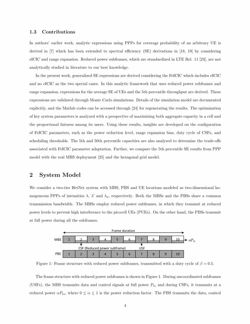
Figure 1: Frame structure with reduced power subframes, transmitted with a duty cycle of β = 0.5.

The frame structure with reduced power subframes is shown in Figure 1. During uncoordinated subframes

(USFs), the MBS transmits data and control signals at full power Ptx and during CSFs, it transmits at a

reduced power αPtx, where 0 ≤ α ≤ 1 is the power reduction factor. The PBS transmits the data, control

4

signals and cell reference symbol with power P ′

tx during all the subframes. Setting α = 0 corresponds to

eICIC; and α = 1 corresponds to no eICIC case.

Define β as the duty cycle of USFs, i.e., ratio of the number of USFs to the total number of sub-frames

in a frame. Then, (1− β) is the duty cycle of CSF/reduced power subframes. Let K and K ′ be the factors

that account for geometrical parameters such as the transmitter and receiver antenna heights of the MBS

and the PBS, respectively. Then, the effective transmitted powers of MBS during USFs is P = PtxK, MBS

during CSFs is αP , and PBS during USF/CSF is P ′ = P ′

txK′. For an arbitrary UE, let the nearest MBS at

a distance r be its macrocell of interest (MOI) and the nearest PBS at a distance r′ be its picocell of interest

(POI). Then, assuming Rayleigh fading channel, the reference symbol received power from the MOI and the

POI are given by,

S(r) =PH

rδ, S′(r′) =

P ′H ′

(r′)δ, (1)

respectively, where the random variables H ∼ Exp(1) and H ′ ∼ Exp(1) account for Rayleigh fading. Define

an interference term, Z, as the total interference power at a UE during USFs from all the MBSs and the

PBSs, excluding the MOI and the POI. Similarly, define Z ′ as the total interference power during CSFs. We

assume that there is no frame synchronization across the MBSs and therefore irrespective of whether the

MOI is transmitting a USF or a CSF, the interference at UE has the same distribution in both cases, and is

independent of both S(r) and S′(r′). Then, an arbitrary UE experiences the following four SIRs:

Γ =S(r)

S′(r′) + Z,→ USF SIR from MOI (2)

Γ′ =S′(r′)

S(r) + Z,→ USF SIR from POI (3)

ΓCSF =αS(r)

S′(r′) + Z,→ CSF SIR from MOI (4)

Γ′

CSF =S′(r′)

αS(r) + Z. → CSF SIR from POI (5)

2.1 UE Association

In (4) and (5), it can be noted that Γcsf and Γ′

csf are directly affected by α and hence their usage will make

the cell selection process dependent on α. Thus, we consider Γ and Γ′ to minimize the dependence of the

cell selection process on α.

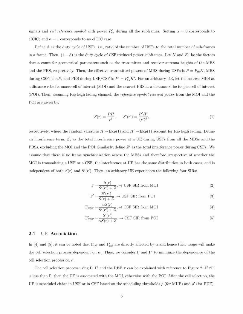
The cell selection process using Γ, Γ′ and the REB τ can be explained with reference to Figure 2. If τΓ′

is less than Γ, then the UE is associated with the MOI, otherwise with the POI. After the cell selection, the

UE is scheduled either in USF or in CSF based on the scheduling thresholds ρ (for MUE) and ρ′ (for PUE).

5

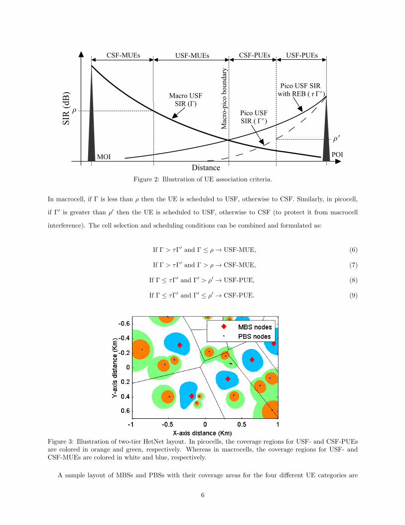
Figure 2: Illustration of UE association criteria.

In macrocell, if Γ is less than ρ then the UE is scheduled to USF, otherwise to CSF. Similarly, in picocell,

if Γ′ is greater than ρ′ then the UE is scheduled to USF, otherwise to CSF (to protect it from macrocell

interference). The cell selection and scheduling conditions can be combined and formulated as:

If Γ > τΓ′ and Γ ≤ ρ → USF-MUE, (6)

If Γ > τΓ′ and Γ > ρ → CSF-MUE, (7)

If Γ ≤ τΓ′ and Γ′ > ρ′ → USF-PUE, (8)

If Γ ≤ τΓ′ and Γ′ ≤ ρ′ → CSF-PUE. (9)

Figure 3: Illustration of two-tier HetNet layout. In picocells, the coverage regions for USF- and CSF-PUEsare colored in orange and green, respectively. Whereas in macrocells, the coverage regions for USF- andCSF-MUEs are colored in white and blue, respectively.

A sample layout of MBSs and PBSs with their coverage areas for the four different UE categories are

6

illustrated in Figure 3. Note that in the related work of [16], the UE association criteria are based on the

average reference symbol received power at UE, where as our model is based on the SIR at UE, it also

encompasses the FeICIC mechanism. In [16], the boundary between the USF-PUEs (picocell area) and the

CSF-PUEs (range expanded area) is fixed due to the fixed transmit power of PBS. On the other hand, in

our approach, the boundary between USF and CSF users can be controlled using ρ in macrocell and ρ′ in

picocell, the parameters which play an important role during optimization as will be shown in Section 5.3.

Using (1)-(5), it can be shown that the two SIRs ΓCSF and Γ′

CSF could be expressed in terms of Γ and

Γ′ as,

Γcsf = αΓ, Γ′

csf =Γ′(1 + Γ)

1 + Γ[α(Γ′ + 1)− Γ′]. (10)

Hence, knowing the statistics of Γ and Γ′, particularly their joint probability density function (JPDF), would

provide a complete picture of the SIR statistics of the HetNet system. We first derive an expression for joint

complementary cumulative distribution function (JCCDF) of Γ and Γ′ in Section 3.1. Then we differentiate

the JCCDF with respect to γ and γ′ to get the expression for JPDF in Section 3.2, which will then be used

for spectral efficiency analysis.

3 Derivation of Joint SINR Distribution

3.1 JCCDF of Γ and Γ′

From (1), we know that S(r) and S′(r′) are exponentially distributed with mean P/rδ and P ′/(r′)δ, respec-

tively. For brevity, substitute S(r) = X and S′(r′) = Y in (2) and (3):

Γ =X

Y + Z, Γ′ =

Y

X + Z. (11)

Using (11) it can be easily shown that the product ΓΓ′ has a maximum value of 1.

Let, R and R′ be the random variables denoting the distances of MOI and POI from a UE. Then, the

JCCDF of Γ and Γ′ conditioned on R = r, R′ = r′ is given by,

P{Γ > γ,Γ′ > γ′∣

∣ R = r, R′ = r′} = EZ

[

P{

X > γ(Y + Z), Y > γ′(X + Z)}

]

,

= EZ

[

∫ +∞

y1

fY (y)

∫ y/γ′−Z

γ(y+Z)

fX(x) dxdy

]

, (12)

7

x

y

y = γ′(x+Z)

x = γ(y+Z)

y1

x1

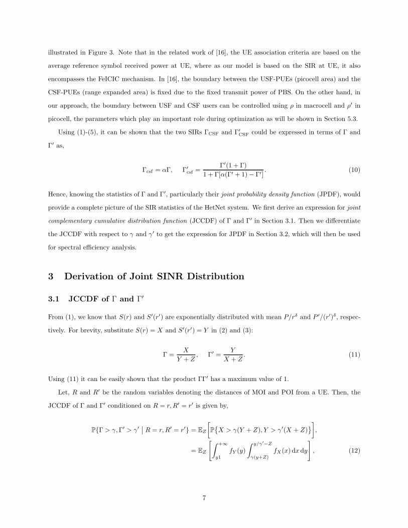
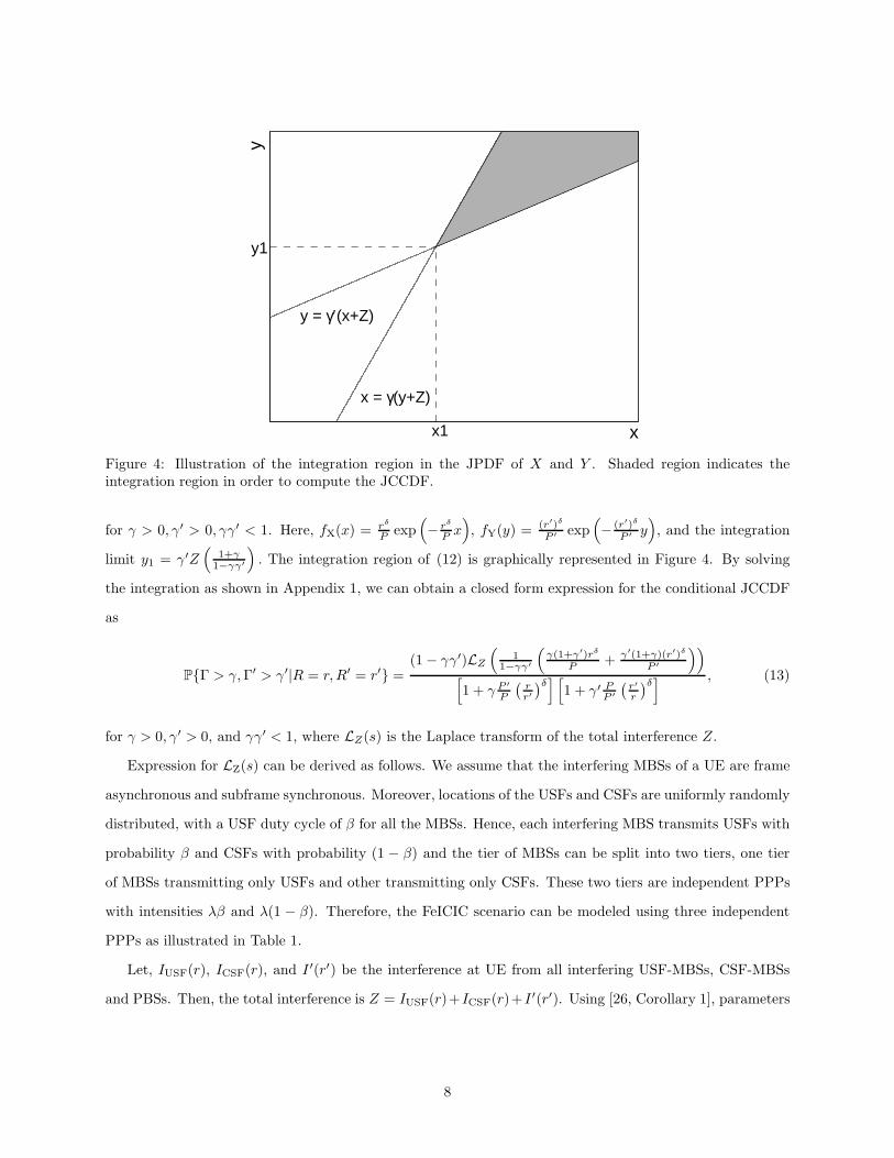
Figure 4: Illustration of the integration region in the JPDF of X and Y . Shaded region indicates theintegration region in order to compute the JCCDF.

for γ > 0, γ′ > 0, γγ′ < 1. Here, fX(x) =rδ

P exp(

− rδ

P x)

, fY(y) =(r′)δ

P ′exp

(

− (r′)δ

P ′y)

, and the integration

limit y1 = γ′Z(

1+γ1−γγ′

)

. The integration region of (12) is graphically represented in Figure 4. By solving

the integration as shown in Appendix 1, we can obtain a closed form expression for the conditional JCCDF

as

P{Γ > γ,Γ′ > γ′|R = r, R′ = r′} =(1− γγ′)LZ

(

11−γγ′

(

γ(1+γ′)rδ

P + γ′(1+γ)(r′)δ

P ′

))

[

1 + γ P ′

P

(

rr′

)δ] [

1 + γ′ PP ′

(

r′

r

)δ] , (13)

for γ > 0, γ′ > 0, and γγ′ < 1, where LZ(s) is the Laplace transform of the total interference Z.

Expression for LZ(s) can be derived as follows. We assume that the interfering MBSs of a UE are frame

asynchronous and subframe synchronous. Moreover, locations of the USFs and CSFs are uniformly randomly

distributed, with a USF duty cycle of β for all the MBSs. Hence, each interfering MBS transmits USFs with

probability β and CSFs with probability (1 − β) and the tier of MBSs can be split into two tiers, one tier

of MBSs transmitting only USFs and other transmitting only CSFs. These two tiers are independent PPPs

with intensities λβ and λ(1 − β). Therefore, the FeICIC scenario can be modeled using three independent

PPPs as illustrated in Table 1.

Let, IUSF(r), ICSF(r), and I ′(r′) be the interference at UE from all interfering USF-MBSs, CSF-MBSs

and PBSs. Then, the total interference is Z = IUSF(r)+ICSF(r)+I ′(r′). Using [26, Corollary 1], parameters

8

Table 1: PPP parameters for USF MBSs, CSF MBSs, and PBSs.

BS type PPP Intensity Tx.

power

Distance of

UE to nearest

BS

USF-MBSs ΦUSF βλ P rCSF-MBSs ΦCSF (1− β)λ αP rPBSs Φ′ λ′ P ′ r′

in Table 1, and assuming δ = 4, we can derive the Laplace transform of Z in (13) to be,

LZ(s) = exp

{

− πβλ√Ps

[

π

2− tan−1

(

r2√Ps

)]

− π(1 − β)λ√αPs

[

π

2− tan−1

(

r2√αPs

)]

− πλ′√P ′s

[

π

2− tan−1

(

(r′)2√P ′s

)]}

. (14)

3.2 JPDF of Γ and Γ′

The conditional JPDF of Γ and Γ′,

fΓ,Γ′

∣

∣R,R′(γ, γ′

∣

∣ r, r′) = P{Γ = γ,Γ′ = γ′|R = r, R′ = r′} (15)

can be derived by differentiating the JCCDF in (13) with respect to γ and γ′. Detailed derivation of

conditional probability JPDF is provided in Appendix 2. Using the theorem of conditional probability we

can write

fΓ,Γ′,R,R′(γ, γ′, r, r′) = fΓ,Γ′

∣

∣R,R′(γ, γ′

∣

∣ r, r′)fR(r)fR′(r′), (16)

where, the PDFs of R and R′ are fR(r) = 2πλre−λπr2 and fR′(r′) = 2πλ′r′e−λ′π(r′)2 , respectively. We can

then express the unconditional JPDF of Γ and Γ′ as,

fΓ,Γ′(γ, γ′) =

∫

∞

dmin

∫

∞

d′

min

fΓ,Γ′,R,R′(γ, γ′, r, r′) dr′ dr

=

∫

∞

dmin

∫

∞

d′

min

fΓ,Γ′

∣

∣R,R′(γ, γ′

∣

∣ r, r′)fR(r)fR′ (r′) dr′ dr, (17)

where, we assume that a UE is served by a BS only if it satisfies the minimum distance constraints: UE

should be located at distances of at least dmin from the MOI and d′min from the POI.

9

4 Spectral efficiency analysis

In this section, the expressions for aggregate and per-user SEs categories are derived. Considering the JPDF

of an arbitrary UE in (17), first the expressions for the probabilities that the UE belongs to each category

are derived. Then, these expressions are used to derive the mean number of UEs of each category in a cell.

These are followed by the derivation of the aggregate SE. Then, per-user SE expressions are obtained by

dividing the aggregate SE by the mean number of UEs.

4.1 MUE and PUE Probabilities

Depending on the SIRs Γ and Γ′, a UE can be one of the four types: USF-MUE, CSF-MUE, USF-PUE or

CSF-PUE. Given that the UE is located at a distance r from its MOI and r′ from its POI, probabilities of

the UE belonging to each type can be found by integrating the conditional JPDF over the regions whose

boundaries are set by the cell selection conditions in (6)-(9). Based on these conditions the integration

regions for different UE categories are shown in Figure 5.

γ′

γ

USF−MUE

CSF−MUE

CSF−PUEUSF−PUE

R2

R1

R3R4

ρ

√

τ

1/√

τ ρ′

γ = τ γ′γ = 1/γ′

Figure 5: Illustration of the integration regions in the JPDF of Γ and Γ′. Shaded regions indicate theintegration regions to compute the probabilities of a UE belonging to different categories.

The probability that a UE is a CSF-MUE can be found by integrating the JPDF over the region R1,

Pcsf =P{Γ > τΓ′,Γ > ρ} =

∫

∞

ρ

∫ min( 1γ, γτ )

0

fΓ,Γ′(γ, γ′) dγ′ dγ. (18)

10

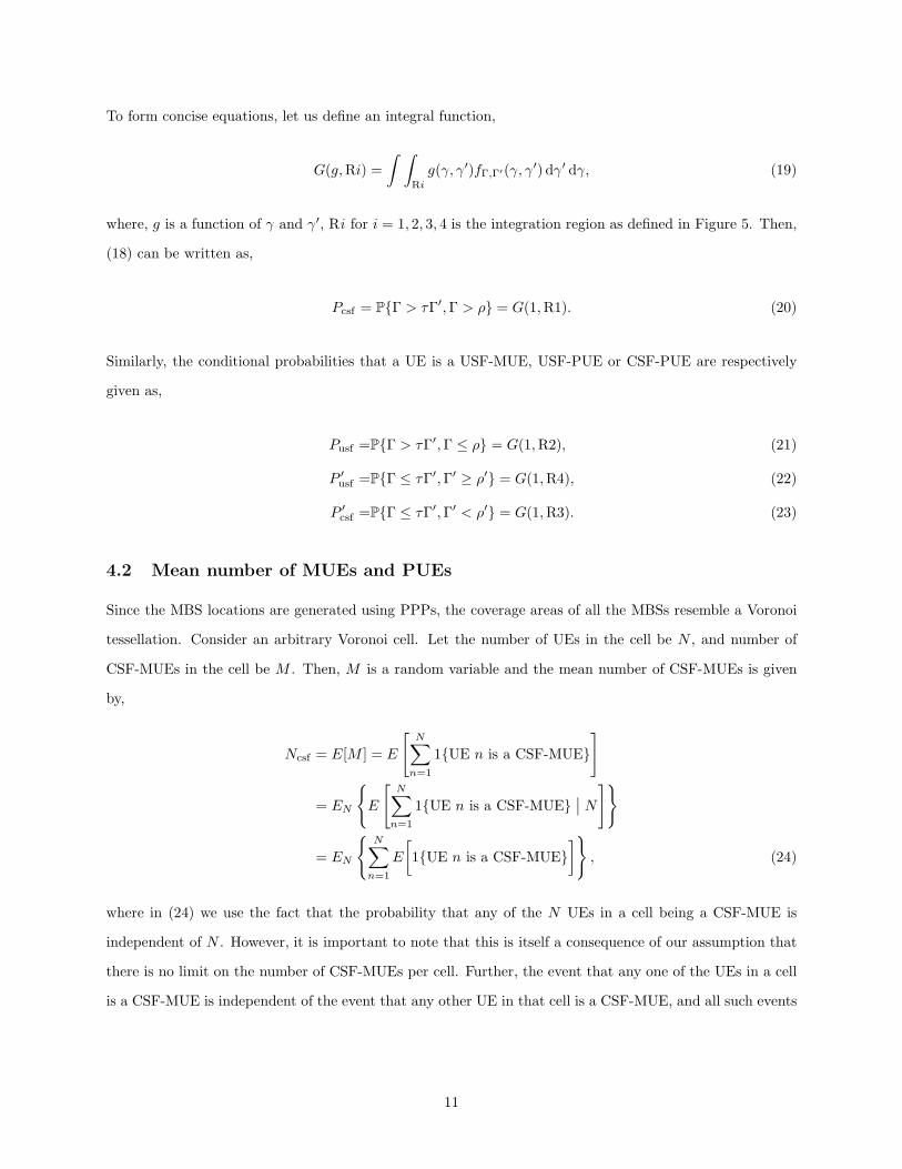
To form concise equations, let us define an integral function,

G(g,Ri) =

∫ ∫

Ri

g(γ, γ′)fΓ,Γ′(γ, γ′) dγ′ dγ, (19)

where, g is a function of γ and γ′, Ri for i = 1, 2, 3, 4 is the integration region as defined in Figure 5. Then,

(18) can be written as,

Pcsf = P{Γ > τΓ′,Γ > ρ} = G(1,R1). (20)

Similarly, the conditional probabilities that a UE is a USF-MUE, USF-PUE or CSF-PUE are respectively

given as,

Pusf =P{Γ > τΓ′,Γ ≤ ρ} = G(1,R2), (21)

P ′

usf =P{Γ ≤ τΓ′,Γ′ ≥ ρ′} = G(1,R4), (22)

P ′

csf =P{Γ ≤ τΓ′,Γ′ < ρ′} = G(1,R3). (23)

4.2 Mean number of MUEs and PUEs

Since the MBS locations are generated using PPPs, the coverage areas of all the MBSs resemble a Voronoi

tessellation. Consider an arbitrary Voronoi cell. Let the number of UEs in the cell be N , and number of

CSF-MUEs in the cell be M . Then, M is a random variable and the mean number of CSF-MUEs is given

by,

Ncsf = E[M ] = E

[

N∑

n=1

1{UE n is a CSF-MUE}]

= EN

{

E

[

N∑

n=1

1{UE n is a CSF-MUE}∣

∣ N

]}

= EN

{

N∑

n=1

E

[

1{UE n is a CSF-MUE}]

}

, (24)

where in (24) we use the fact that the probability that any of the N UEs in a cell being a CSF-MUE is

independent of N . However, it is important to note that this is itself a consequence of our assumption that

there is no limit on the number of CSF-MUEs per cell. Further, the event that any one of the UEs in a cell

is a CSF-MUE is independent of the event that any other UE in that cell is a CSF-MUE, and all such events

11

have the same probability of occurrence, namely Pcsf given in (20). Then,

Ncsf = EN

{

N∑

n=1

Pcsf

}

= EN [NPcsf ] = Pcsf E[N ]. (25)

Using [27, Lemma 1], it can be shown that the mean number of UEs in a Voronoi cell is λu/λ. Therefore,

the mean number of CSF-MUEs in a cell are given by,

Ncsf =Pcsfλu

λ. (26)

Similarly, the mean number of USF-MUEs, USF-PUEs and CSF-PUEs are respectively given by,

Nusf =Pusfλu

λ, N ′

usf =P ′

usfλu

λ′, N ′

csf =P ′

csfλu

λ′. (27)

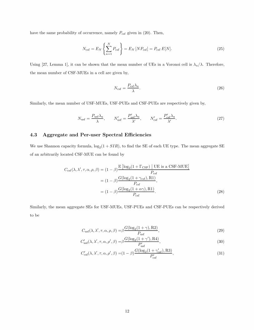
4.3 Aggregate and Per-user Spectral Efficiencies

We use Shannon capacity formula, log2(1 + SIR), to find the SE of each UE type. The mean aggregate SE

of an arbitrarily located CSF-MUE can be found by

Ccsf(λ, λ′, τ, α, ρ, β) = (1− β)

E[

log2(1 + ΓCSF)∣

∣ UE is a CSF-MUE]

Pcsf

= (1− β)G(log2(1 + γcsf),R1)

Pcsf,

= (1− β)G(log2(1 + αγ),R1)

Pcsf. (28)

Similarly, the mean aggregate SEs for USF-MUEs, USF-PUEs and CSF-PUEs can be respectively derived

to be

Cusf(λ, λ′, τ, α, ρ, β) =β

G(log2(1 + γ),R2)

Pusf, (29)

C′

usf(λ, λ′, τ, α, ρ′, β) =β

G(log2(1 + γ′),R4)

P ′

usf

, (30)

C′

csf(λ, λ′, τ, α, ρ′, β) =(1− β)

G(log2(1 + γ′

csf),R3)

P ′

csf

, (31)

12

where, γ′

csf =γ′(1+γ)

1+γ[α(γ′+1)−γ′] . Then the corresponding per-user SEs are

Cu,usf(λ, λ′, τ, α, ρ, β) =

λ Cusf(λ, λ′, τ, α, ρ, β)

λu Pusf, (32)

Cu,csf(λ, λ′, τ, α, ρ, β) =

λ Ccsf(λ, λ′, τ, α, ρ, β)

λu Pcsf, (33)

C′

u,usf(λ, λ′, τ, α, ρ′, β) =

λ′ C′

usf(λ, λ′, τ, α, ρ′, β)

λu P ′

usf

, (34)

C′

u,csf(λ, λ′, τ, α, ρ′, β) =

λ′ C′

csf(λ, λ′, τ, α, ρ′, β)

λu P ′

csf

. (35)

4.4 5th Percentile Throughput

The 5th percentile throughput reflects the throughput of cell-edge UEs. Typically the cell-edge UEs expe-

rience high interference and analyzing their throughput provides important information about the fairness

among the users in a cell and the system performance.

Consider the JPDF expression in (17). The integration regions of the JPDF for different UE categories

are shown in Figure 5. The SIR PDF of USF-MUEs can be evaluated by integrating the JPDF over γ′ in

the region R2,

fΓ(γ) = P{Γ = γ∣

∣ UE is a USF-MUE} =

∫ min( γτ, 1γ )

0

fΓ,Γ′(γ, γ′) dγ′, (36)

for 0 ≤ γ ≤ ρ. The CDF expression can be derived as

FΓ(γusf) = P{Γ ≤ γusf∣

∣ UE is a USF-MUE}

=

∫ γusf

0

fΓ(γ) dγ =

∫ γusf

0

∫ min( γτ, 1γ )

0

fΓ,Γ′(γ, γ′) dγ′ dγ, (37)

for 0 ≤ γusf ≤ ρ and, the CDF of throughput of the USF-MUEs can be derived as a function of FΓ(γusf) in

(37) as,

FCusf(cusf) = P{CUSF ≤ cusf

∣

∣ UE is a USF-MUE}

= P{log2(1 + Γusf) ≤ cusf∣

∣ UE is a USF-MUE},

= P{Γusf ≤ (2cusf − 1)∣

∣ UE is a USF-MUE}

= FΓ(2cusf − 1), (38)

for 0 ≤ cusf ≤ log2(1 + ρ). By using the CDF plots, the 5th percentile throughput of USF-MUEs can easily

13

be found as the value at which the CDF is equal to 0.05. Similarly, the 5th percentile throughput of other

three UE categories can also be found.

5 Numerical and Simulation Results

The average SE and 5th percentile throughput expressions derived in the earlier sections are validated

using a Monte Carlo simulation model built in Matlab. Validation of the PPP capacity results for a HetNet

scenario with range expansion and reduced power subframes is a non-trivial task. In this section, details of the

simulation approach used for validating the PPP analyses are explicitly documented to enable reproducibility.

Matlab codes for the simulation model and the theoretical analysis can be downloaded from [24].

−6 −4 −2 0 2 4 6−6

−4

−2

0

2

4

6

Y−

axis

dis

tanc

e (K

m)

X−axis distance (Km)

UEsPBSsMBSs

Area A

Area Au

Figure 6: Simulation layout.

5.1 Simulation Methodology for verifying PPP Model

Algorithm used in simulation to find the aggregate and per-user SEs is described below.

1. The X- and Y-coordinates of MBSs, PBSs and UEs are generated using uniformly distributed random

variables. The number of MBS and PBS location marks are λA and λ′A respectively, where, A is the

assumed geographical area that is square in shape as illustrated in Figure 6.

14

2. The UE locations are constrained within a smaller area Au which is aligned at center of the main

simulation area A to avoid the UEs to be located at the edges. In the PPP analysis, the area is

assumed to be infinite. But in simulation, this scenario is approximated by making A sufficiently

larger than Au. The number of UEs is λuAu.

3. The MOI (closest MBS) and POI (closest PBS) for each UE is identified. The minimum distance

constraints are applied by discarding the UEs that are closer than dmin(d′

min) from their respective

MOIs (POIs).

4. The SIRs Γ, Γ′, ΓCSF, Γ′

CSF are calculated for each UE using (2)-(5).

5. The UEs are classified as USF-MUEs, CSF-MUEs, USF-PUEs and CSF-PUEs using the conditions in

(6)-(9).

6. The MUEs (PUEs) which share the same MOI (POI) are grouped together to form the macro- and

pico-cells.

7. The SEs of all the UEs are calculated. In a cell, SE of a USF-MUE i is calculated using

β log2(1+Γi)/ (No. of USF-MUEs in the cell). The SEs of other UE types are calculated using similar

formulations.

8. The aggregate capacity of each UE type is calculated in all the cells.

9. Mean aggregate capacity and mean number of UEs of each type are calculated by averaging over all

the cells.

10. The per-user SE of each UE type are calculated by (mean aggregate capacity)/(mean number of UEs).

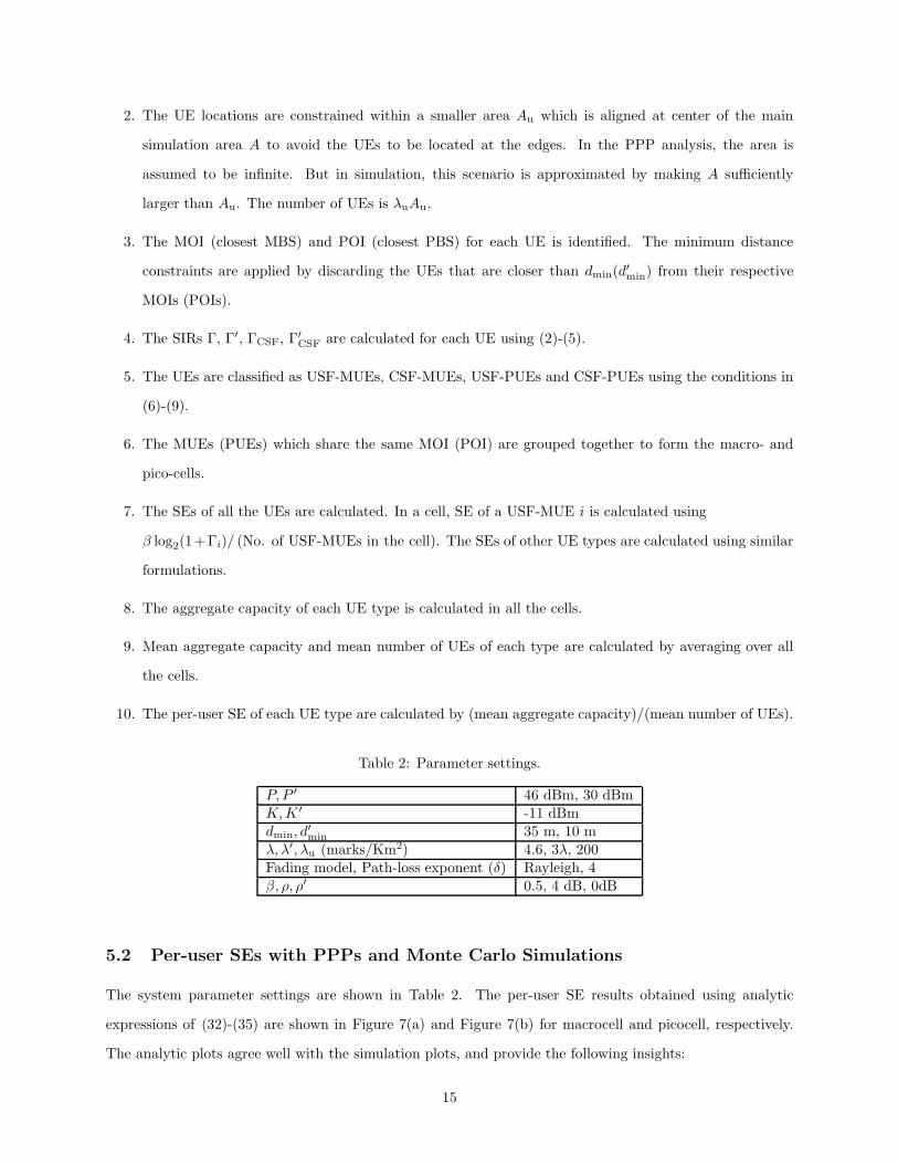
Table 2: Parameter settings.

P, P ′ 46 dBm, 30 dBmK,K ′ -11 dBmdmin, d

′

min 35 m, 10 mλ, λ′, λu (marks/Km2) 4.6, 3λ, 200Fading model, Path-loss exponent (δ) Rayleigh, 4β, ρ, ρ′ 0.5, 4 dB, 0dB

5.2 Per-user SEs with PPPs and Monte Carlo Simulations

The system parameter settings are shown in Table 2. The per-user SE results obtained using analytic

expressions of (32)-(35) are shown in Figure 7(a) and Figure 7(b) for macrocell and picocell, respectively.

The analytic plots agree well with the simulation plots, and provide the following insights:

15

0 5 10 150

5

10

15

20

25

30

35

40

45

Range expansion bias, τ (in dB)

Per

−us

er m

acro

cell

SE

x λ

u (bp

s/he

rtz)

α = 0 (Sim)

α = 0 (PPP)

α = 0.5 (Sim)

α = 0.5 (PPP)

α = 1 (Sim)

α = 1 (PPP)

CSF−MUEs

USF−MUEs

(a)

0 5 10 150

10

20

30

40

50

60

70

80

90

100

Range expansion bias, τ (in dB)

Per

−us

er p

icoc

ell S

E x

λu (

bps/

hert

z)

α = 0 (Sim)

α = 0 (PPP)

α = 0.5 (Sim)

α = 0.5 (PPP)

α = 1 (Sim)

α = 1 (PPP)

USF−PUEs

CSF−PUEs

(b)

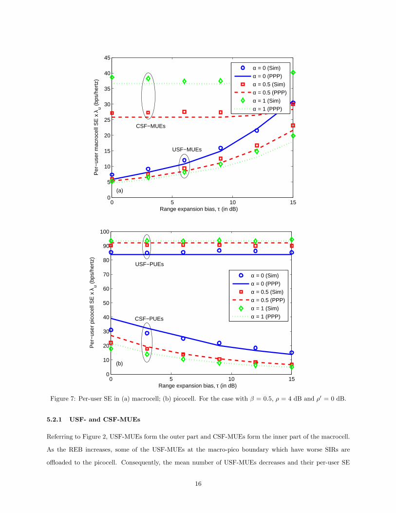
Figure 7: Per-user SE in (a) macrocell; (b) picocell. For the case with β = 0.5, ρ = 4 dB and ρ′ = 0 dB.

5.2.1 USF- and CSF-MUEs

Referring to Figure 2, USF-MUEs form the outer part and CSF-MUEs form the inner part of the macrocell.

As the REB increases, some of the USF-MUEs at the macro-pico boundary which have worse SIRs are

offloaded to the picocell. Consequently, the mean number of USF-MUEs decreases and their per-user SE

16

increases as shown in Figure 7(a).

The mean number of CSF-MUEs are not affected by τ as long as√τ ≤ ρ. Considering Figure 5, it can

be noted that if√τ = ρ, the line γ = τγ′ intersects the boundary of region R1. Hence, if τ is increased

further such that√τ > ρ, the area of R1 decreases and thereby decreases the mean number of CSF-MUEs.

Therefore, the per-user SE of CSF MUEs remains constant as long as√τ ≤ ρ, and increases if τ crosses this

limit as shown in Figure 7(a).

On the other hand, as the α increases, the transmit power of all the interfering MBSs increases during

CSFs, hence it increases the interference power Z at all the UEs. This causes the SIRs of USF-MUEs (Γ),

USF-PUEs (Γ′) and CSF-PUEs (Γ′

csf) to decrease, which can be noted in (2), (3), and (5), respectively.

However, the SIRs of CSF-MUEs (Γcsf) would increase (despite of increased interference) because of the

increase in received signal power (due to higher α) which can be noted in (4). Considering (6) and (7),

since ρ is a constant, the degradation in Γ causes the number of USF-MUEs to increase and CSF-MUEs

to decrease. Consequently, the per-user SE of USF-MUEs decreases and that of CSF-MUEs increases for

increasing α, as shown in Figure 7(a).

5.2.2 USF- and CSF-PUEs

As the REB increases, the mean number of USF-PUEs remains constant if ρ′ > 1/√τ because the area of

region R4 in Figure 5 is unaffected by the value of τ . Therefore, the per-user SE of USF-PUEs also remain

constant for increasing REB as shown in Figure 7(b). With increasing REB, some MUEs are offloaded to

the picocell and become CSF-PUEs. But, these UEs are located at cell-edges and have low SIRs. Hence the

per-user SE of CSF-PUEs decreases as shown in Figure 7(b).

On the other hand, as the α increases, the transmit power of all the interfering MBSs increases during

CSFs causing Γ, Γ′ and Γ′

csf to decrease and Γcsf to increase, as explained previously. Considering (8) and

(9), since ρ′ is a constant the degradation in Γ′ causes the number of USF-PUEs to decrease and CSF-PUEs

to increase. Consequently, the per-user SE of USF-PUEs increases and that of CSF-PUEs decreases for

increasing α, as shown in Figure 7(b).

5.3 Optimization of System Parameters to Achieve Maximum Capacity and

Proportional Fairness

The five parameters τ, α, β, ρ, and ρ′ are the key system parameters that are critical to the satisfactory

performance of the HetNet system. The goal of these parameter settings is to maximize the aggregate

capacity in a cell while providing proportional fairness among the users.

17

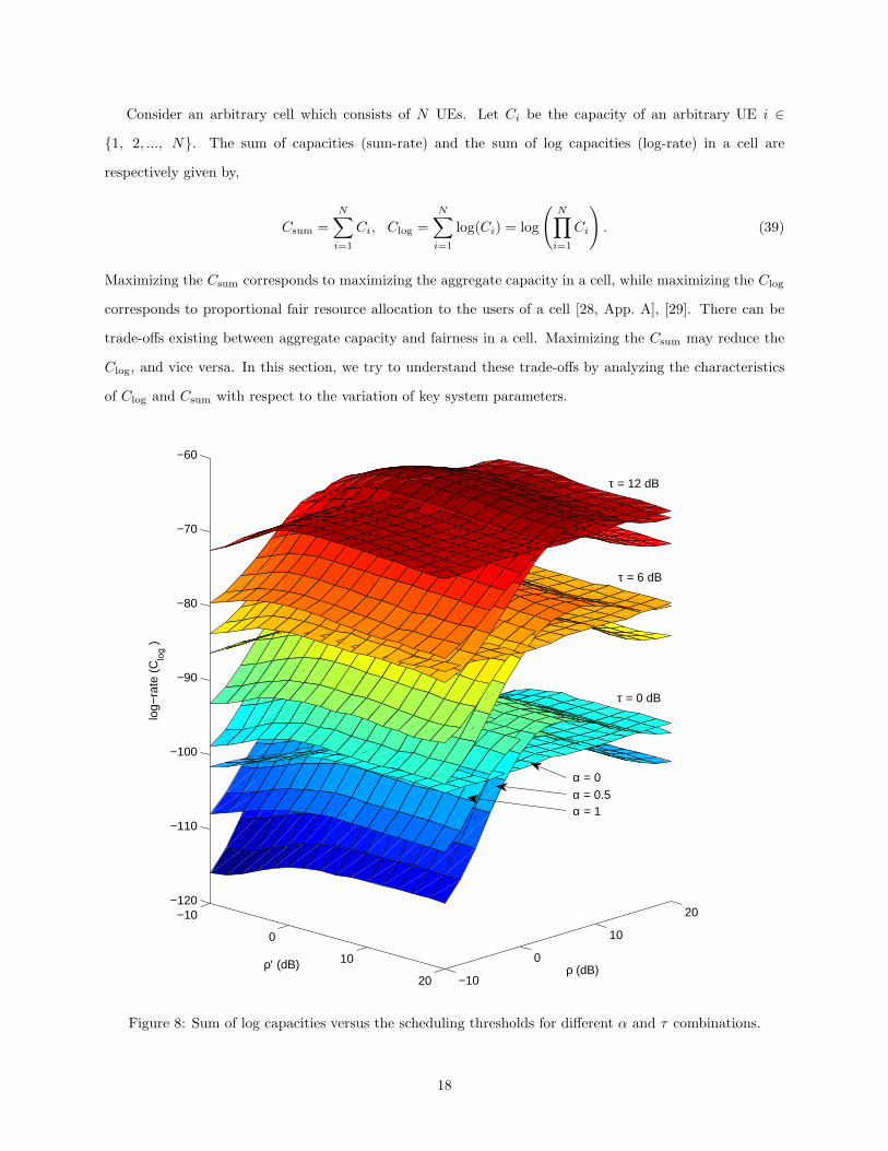
Consider an arbitrary cell which consists of N UEs. Let Ci be the capacity of an arbitrary UE i ∈

{1, 2, ..., N}. The sum of capacities (sum-rate) and the sum of log capacities (log-rate) in a cell are

respectively given by,

Csum =

N∑

i=1

Ci, Clog =

N∑

i=1

log(Ci) = log

(

N∏

i=1

Ci

)

. (39)

Maximizing the Csum corresponds to maximizing the aggregate capacity in a cell, while maximizing the Clog

corresponds to proportional fair resource allocation to the users of a cell [28, App. A], [29]. There can be

trade-offs existing between aggregate capacity and fairness in a cell. Maximizing the Csum may reduce the

Clog, and vice versa. In this section, we try to understand these trade-offs by analyzing the characteristics

of Clog and Csum with respect to the variation of key system parameters.

−10

0

10

20 −10

0

10

20−120

−110

−100

−90

−80

−70

−60

ρ (dB)ρ′ (dB)

log−

rate

(C

log )

τ = 0 dB

τ = 6 dB

τ = 12 dB

α = 0

α = 1 α = 0.5

Figure 8: Sum of log capacities versus the scheduling thresholds for different α and τ combinations.

18

We attempt to achieve the proportional fairness by optimizing the five key system parameters to maximize

the Clog. The variation of Clog with respect to ρ, ρ′, α, τ is shown in Figure 8, for β = 0.5. These plots are

obtained through the Monte Carlo simulations and each surface plot is the variation of Clog with respect to

ρ and ρ′ for a fixed value of α and τ . The optimum scheduling thresholds ρ∗ and ρ′∗ that maximizes the

Clog are dependent on the values of α and τ .

0 0.2 0.4 0.6 0.8 10

5

10

15

20

ρ *

(dB

)

0 0.2 0.4 0.6 0.8 1−5

0

5

10

15

Power reduction factor, α

ρ′ *

(dB

)

τ = 0 dBτ = 6 dBτ = 12 dB

τ = 0 dBτ = 6 dBτ = 12 dB

(a)

(b)

Figure 9: Optimized scheduling thresholds versus α for different τ (a) in macrocell; (b) in picocell. Withλ = 4.6 marks/Km2 and λ′ = 13.8 marks/Km2.

Figure 9 shows the plots of ρ∗ and ρ′∗ as the functions of α and τ . The markers show the simulation

results while the dotted lines show the smoother estimation obtained using the curve fitting tool in MATLAB.

For small α values, the optimum threshold ρ∗ has higher values as shown in Figure 9(a), and according to

(7) this causes very few MUEs that have Γ > ρ∗ to be scheduled during CSFs. This makes sense because

MBS transmit power during CSFs is very low for small α and hence the number of CSF-MUEs which can be

covered is also less. On the other hand, for higher α values, MBS transmits with higher power level during

CSFs and can cover larger number of CSF-MUEs. Therefore, to improve the fairness proportionally, the

optimal ρ∗ value decreases with increasing α so that more MUEs are scheduled during CSFs.

In the picocell, with increasing α the CSF-PUEs at the cell edges will experience higher interference from

the MBSs. Then, more PUEs should be scheduled during USFs to improve proportional fairness. Likewise,

decreasing ρ′∗ in Figure 9(b) indicates that more PUEs are scheduled during USFs as per (8).

19

0 0.2 0.4 0.6 0.8 1−100

−95

−90

−85

−80

−75

−70

−65

−60

Power reduction factor, α

Clo

g

τ = 0 dBτ = 6 dBτ = 12 dB

Ideal range forproportional fairness

Figure 10: Clog versus α with optimum scheduling thresholds ρ∗ and ρ′∗. With λ = 4.6 marks/Km2 andλ′ = 13.8 marks/Km2.

The Clog with optimum scheduling thresholds ρ∗ and ρ′∗ is plotted in Figure 10. Higher the Clog, better

is the proportional fairness. It is important to note that the range expansion bias, τ , has a significant effect

on proportional fairness. The Clog increases from −40 to −28 when τ is increased from 0 db to 12 dB.

Compared to τ , α has a smaller effect on the proportional fairness. When α is set to zero which corre-

sponds to the eICIC, Clog is at its minimum. It shows that eICIC provides minimum proportional fairness.

Figure 10 moreover shows that setting α = 1 which corresponds to no eICIC, also does not provide maximum

Clog. An α setting between 0.125 and 0.5 maximizes the Clog and hence the proportional fairness.

The characteristics of Csum with optimum scheduling thresholds is shown in Figure 11. As the τ increases,

Csum decreases, which is the opposite effect when compared to the Clog in Figure 10. This shows the trade-

off between the aggregate capacity and the proportional fairness. Increasing the τ would increase the

proportional fairness but decrease the aggregate capacity, and vice versa.

Comparing Figures 10 and 11 also explains the trade-off associated with setting α. A very small value,

0 < α < 0.125, provides larger Csum but smaller Clog, which is better from an aggregate capacity point

of view. Setting 0.125 ≤ α ≤ 0.5 is better from a fairness point of view. Any value of α > 0.5 is not

recommended since it degrades the aggregate capacity as shown in Figure 11, decreases the proportional

fairness as shown in Figure 10, and consumes higher transmit power by the MBSs. Setting α = 0 as in the

eICIC case would reduce both Csum and Clog drastically.

The implications in Figures 10 and 11 can be seen from a different perspective by using the 5th percentile

20

0 0.2 0.4 0.6 0.8 14

4.5

5

5.5

6

6.5

7

Power reduction factor, α

Csu

m

τ = 0 dBτ = 6 dBτ = 12 dB

ideal range foraggregate capacity

Figure 11: Csum versus α with optimum scheduling thresholds ρ∗ and ρ′∗. With λ = 4.6 marks/Km2 andλ′ = 13.8 marks/Km2.

0.045 0.05 0.055 0.06 0.065 0.07 0.075 0.08 0.0853

4

5

6

7

8

9x 10

−3

50th percentile SE (bps/Hz)

5th

perc

entil

e S

E (

bps/

Hz)

τ = 0 dB (sim)

τ = 6 dB (sim)

τ = 12 dB (sim)

α = 0

α = 1

α = 1

α = 1

α = 0

α = 0.125

α = 0

Figure 12: 5th percentile capacity versus 50th percentile capacity. With λ = 4.6 marks/Km2 and λ′ =13.8 marks/Km2.

SE versus 50th percentile SE graph shown in Figure 12. It shows that increasing the τ from 6 dB to 12 dB

improves the 50th percentile SE, but degrades the 5th percentile SE. This illustrates the trade-off between the

21

5th and 50th percentile SEs, which is analogous to the trade-off between aggregate capacity and proportional

fairness among the users, as explained in the previous paragraphs. Figure 12 also shows that α has a notable

effect on the 5th and 50th percentile SEs.

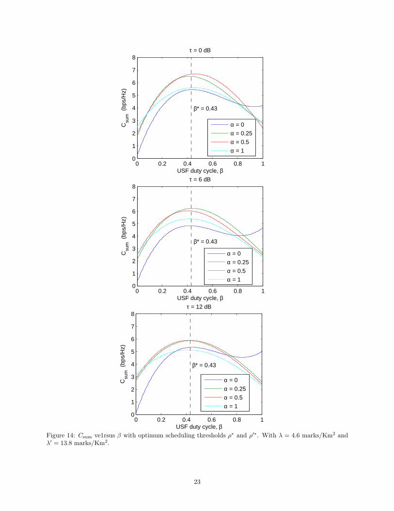
5.4 Impact of the Duty Cycle of Uncoordinated Subframes

In the results of Figures 9–12, β was set to 0.5 and we next show the effect of varying β on Clog and Csum.

Introducing β into the optimization problem makes it difficult to visualize the results due to the addition of

one more dimension. Therefore, we use the optimized scheduling thresholds, ρ∗ and ρ′∗, and analyze Clog

and Csum as the functions β, α and τ . Figures 13 and 14 show the Clog versus β and the Csum versus β,

respectively for different values of α and τ . The variation of Clog with respect to β is not significant, except

for α = 0. Whereas, the variation of Csum with respect to β is significant.

0.1 0.2 0.3 0.4 0.5 0.6 0.7 0.8 0.9−115

−110

−105

−100

−95

−90

−85

−80

−75

−70

−65

−60

USF duty cycle, β

Clo

g

α = 0

α = 0.25

α = 0.5

α = 1

τ = 12 dB

τ = 6 dB

τ = 0 dB

Figure 13: Clog versus β with optimum scheduling thresholds ρ∗ and ρ′∗. With λ = 4.6 marks/Km2 andλ′ = 13.8 marks/Km2.

When α = 0, the Clog value decreases rapidly for β < 0.5. Nevertheless, α = 0 is shown to have poor

performance in the previous paragraphs and hence it is not recommended. For other values of α, variation

in β does not affect the Clog significantly, which shows that by using a fixed value of β, proportional fairness

can be achieved by optimizing (to maximize Clog) the scheduling thresholds. Figure 14 shows that fixing β

approximately to 0.43 maximizes the Csum irrespective of α and τ , provided the scheduling thresholds are

optimized to maximize Clog.

22

0 0.2 0.4 0.6 0.8 10

1

2

3

4

5

6

7

8τ = 0 dB

Csu

m (

bps/

Hz)

USF duty cycle, β

α = 0

α = 0.25

α = 0.5

α = 1

β* = 0.43

0 0.2 0.4 0.6 0.8 10

1

2

3

4

5

6

7

8

Csu

m (

bps/

Hz)

USF duty cycle, β

τ = 6 dB

α = 0

α = 0.25

α = 0.5

α = 1

β* = 0.43

0 0.2 0.4 0.6 0.8 10

1

2

3

4

5

6

7

8

Csu

m (

bps/

Hz)

USF duty cycle, β

τ = 12 dB

α = 0

α = 0.25

α = 0.5

α = 1

β* = 0.43

Figure 14: Csum ve1rsus β with optimum scheduling thresholds ρ∗ and ρ′∗. With λ = 4.6 marks/Km2 andλ′ = 13.8 marks/Km2.

23

In [16], the boundary of CSF-PUEs that form the inner region of picocell (excluding the range expansion

region) is fixed due to the fixed transmit power of PBS. The association bias and resource partitioning

fraction parameters are used as the variables to be optimized. It is analogous for us to have a fixed ρ′ and

optimize β and τ . But in contrast, we fix the β for simplicity and optimize the other four parameters, since

coordinating β among the cells through the X2 interface is complex and adds to communication overhead in

the backhaul.

5.5 5th Percentile Throughput

Using the expressions derived in Section 4.4, the 5th percentile throughput versus α for different τ is shown

in Figure 15(a) for MUEs, and in Figure 15(b) for PUEs. As the α increases, MBSs transmit at higher power

level during CSFs and the UEs of all types experience a higher interference power. However, the received

signal power at CSF-MUEs increases with α and results in improved 5th percentile throughput as shown

in Figure 15(a). But, the SIRs of USF-MUEs and USF/CSF-PUEs degrade due to higher interference and

therefore their 5th percentile throughput decreases with increase in α as shown in Figures 15(a) and 15(b).

Increasing the REB, τ , causes the USF-MUEs with poor SIR, located at the edge of macrocell, to be

offloaded to the picocell and thereby increasing the 5th percentile throughput of USF-MUEs as shown in

Figure 15(a). The offloaded UEs in picocell are scheduled during CSFs and due to their poor SIR the 5th

percentile throughput of CSF-PUEs decreases as shown in Figure 15(b).

5.6 Comparison with Real BS Deployment

We obtained the data of real BS locations in United Kingdom from an organization [25] where the mobile

network operators have voluntarily provided the information of location and operating characteristics of

individual BSs. The data set in [25] was last updated in May 2012, and it provides exact locations of the

BSs. Also, the BSs of different operators can be distinguished.

In this section, we compare the 5th percentile SE results from the PPP model with that of the real BS

deployment and hexagonal grid model. The real MBS locations of two different operators in a 15× 15 km2

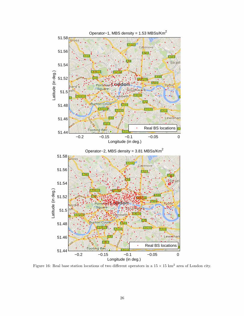
area of London city were obtained from [25] as shown in Figure 16. In this area, the average BS densities

of the two operators were found to be 1.53 MBSs/km2 and 2.04 MBSs/km2. To have a fair comparison, the

MBS locations for hexagonal grid and PPP models were also generated with the same densities. The PBS

locations were generated randomly using another PPP model. The parameters τ = 6 dB, α = 0.5, β = 0.5,

ρ = 4 dB, ρ′ = 12 dB, and Ptx = 46 dBm were fixed while the PBS density λ′ was varied to analyze its effect

on the 5th percentile SE.

24

0 0.2 0.4 0.6 0.8 10

0.5

1

1.5

2

2.5

Power reduction factor, α (a)

5th

perc

entil

e th

roug

hput

(bp

s/H

z)

τ = 0 dB (Sim)

τ = 0 dB (PPP)

τ = 6 dB (Sim)

τ = 6 dB (PPP)

τ = 12 dB (Sim)

τ = 12 dB (PPP)

USF−MUEs

CSF−MUEs

0 0.2 0.4 0.6 0.8 10

0.5

1

1.5

2

2.5

3

3.5

4

4.5

5

Power reduction factor, α (b)

5th

perc

entil

e th

roug

hput

(bp

s/H

z)

τ = 0 dB (Sim)

τ = 0 dB (PPP)

τ = 6 dB (Sim)

τ = 6 dB (PPP)

τ = 12 dB (Sim)

τ = 12 dB (PPP)

CSF−PUEs

USF−PUEs

Figure 15: 5th percentile throughput (a) in macrocell; (b) in picocell. With λ = 4.6 marks/Km2 andλ′ = 13.8 marks/Km2.

The plots of 5th percentile SE versus PBS density are shown in Figure 17 for the two operators. The

5th percentile SE of operator-2 is better than that of operator-1 since the former has higher MBS density.

As expected, the 5th percentile SE improves with the increase in PBS density. It can also be observed

that increasing the PBS transmit power P ′ from 10 dBm to 30 dBm will result into almost twice the 5th

percentile SE. Since hexagonal grid model is an ideal case, it has the best 5th percentile SE and forms an

25

−0.2 −0.15 −0.1 −0.05 051.44

51.46

51.48

51.5

51.52

51.54

51.56

51.58

Longitude (in deg.)

Latit

ude

(in d

eg.)

Real BS locations

Operator−1, MBS density = 1.53 MBSs/Km2

−0.2 −0.15 −0.1 −0.05 051.44

51.46

51.48

51.5

51.52

51.54

51.56

51.58

Longitude (in deg.)

Latit

ude

(in d

eg.)

Operator−2, MBS density = 3.81 MBSs/Km2

Real BS locations

Figure 16: Real base station locations of two different operators in a 15× 15 km2 area of London city.

26

0 5 10 15 200

0.005

0.01

0.015

0.02

PBS density to MBS density ratio, λ′ /λ

5th

perc

entil

e S

E (

bps/

hert

z)

Hex−gridReal MBSRandom (PPP)

P′ = 30 dBm

P′ = 10 dBm

Operator−1, MBS density = 1.53 MBSs/Km2

0 5 10 15 200

0.005

0.01

0.015

0.02

0.025

0.03

0.035

PBS density to MBS density ratio, λ′ /λ

5th

perc

entil

e S

E (

bps/

hert

z)

Hex−gridReal MBSRandom (PPP)

P′ = 10 dBm

P′ = 30 dBm

Operator−2, MBS density = 3.81 MBSs/Km2

Figure 17: 5th percentile SE versus PBS density.

upper bound. The PPP model has the worse 5th percentile SE and forms a lower bound. The real MBS

deployment is usually planned and hence it is not completely random in nature. On the other hand, it is

also not equivalent to the idealized hexagonal grid model due to the practical constraints involved during

27

the deployment. Hence, the 5th percentile SE of real MBS deployment lies in between the two bounds of

hexagonal grid and random deployments.

6 Conclusion

In this paper, spectral efficiency and 5th percentile throughput expressions are derived for HetNets with

reduced power subframes and range expansion. These expressions are validated using the Monte Carlo

simulations. Joint optimization of the key system parameters, such as range expansion bias, power reduction

factor, scheduling thresholds, and duty cycle of reduced power subframes, is performed to achieve maximum

aggregate capacity and proportional fairness among users. Our analysis shows that under optimum parameter

settings, the HetNet with reduced power subframes yields better performance than that with almost blank

subframes (eICIC) in terms of both aggregate capacity and proportional fairness. However, transmitting

the reduced power subframes with greater than half the maximum power proved to be inefficient because

it degrades both the aggregate capacity and the proportional fairness. Increasing the range expansion bias

improves the proportional fairness but degrades the aggregate capacity. In case of eICIC, the duty cycle

of almost blank subframes has a significant effect on the fairness, but with reduced power subframes and

optimized scheduling thresholds, duty cycle has a limited effect on fairness. Hence, fixing the duty cycle and

optimizing the scheduling thresholds is preferable since it avoids the overhead of coordinating the duty cycle

among the cells through the X2 interface. We also compared the 5th percentile SE results from PPP model

with that of real BS deployment and hexagonal grid model. We observed that the hex grid model forms the

upper bound while the PPP model forms the lower bound. Increasing the PBS density or the PBS transmit

power would improve the 5th percentile SE.

28

Appendix 1 Derivation of JCCDF Expression

This part of the appendix derives closed form equation for the JCCDF in (12). Let us start by rewriting the

JCCDF expression,

P{Γ > γ,Γ′ > γ′|R = r, R′ = r′} = EZ

[

∫ +∞

y1

fY(y)

∫ y/γ′−Z

γ(y+Z)

fX(x) dxdy

]

(40)

where,

fX(x) = λx exp(−λxx) and fY(y) = λy exp(−λyy); (41)

λx =rδ

Pand λy =

(r′)δ

P ′. (42)

The inner integral in (40) can be derived as,

∫ y/γ′−Z

γ(y+Z)

fX(x) dx = exp [−λxγ(y + Z)]− exp

[

−λx

(

y

γ′− Z

)]

. (43)

Then, the outer integral in (40) can be derived as,

∫ +∞

y1

fY(y)

∫ y/γ′−Z

γ(y+Z)

fX(x) dxdy =λy

∫ +∞

y1

exp[−λyy − λxγ(y + Z)] dy − λy

∫ +∞

y1

exp

[

−λyy − λx

(

y

γ′− Z

)]

dy. (44)

The first term in right hand side (RHS) of (44) can be evaluated as,

λy

∫ +∞

y1

exp[−λyy − λxγ(y + Z)] dy =1

1 + γλx

λy

exp

[−λxγZ(1 + γ′)− λyγ′Z(1 + γ)

1− γγ′

]

. (45)

The second term in RHS of (44) can be evaluated as,

λy

∫ +∞

y1

exp

[

−λyy − λx

(

y

γ′− Z

)]

dy =1

1 + λx

γ′λy

exp

[−λxγZ(1 + γ′)− λyγ′Z(1 + γ)

1− γγ′

]

. (46)

By substituting (45) and (46) in the first and second terms of (44) respectively, we get

∫ +∞

y1

fY(y)

∫ y/γ′−Z

γ(y+Z)

fX(x) dxdy =

(

1

1 + γλx

λy

− 1

1 + λx

γ′λy

)

exp

[−λxγZ(1 + γ′)− λyγ′Z(1 + γ)

1− γγ′

]

. (47)

29

Substituting (47) in (40) and using (42) we get,

P{Γ > γ,Γ′ > γ′|R = r, R′ = r′}

=

(

1

1 + γ P ′

P

(

rr′

)δ− 1

1 + γ′ PP ′

(

r′

r

)δ

)

EZ

[

exp

(

−Zγ(1+γ′)rδ

P + γ′(1+γ)(r′)δ

P ′

1− γγ′

)]

(48)

Using the definition of Laplace transform, EZ [exp(−Zs)] = LZ(s), and further simplification, we get

P{Γ > γ,Γ′ > γ′|R = r, R′ = r′} =(1− γγ′)LZ

(

11−γγ′

(

γ(1+γ′)rδ

P + γ′(1+γ)(r′)δ

P ′

))

[

1 + γ P ′

P

(

rr′

)δ] [

1 + γ′ PP ′

(

r′

r

)δ] . (49)

Appendix 2 Derivation of JPDF Expression

Assuming δ = 4, the JCCDF expression in (49) can be rewritten as,

P{Γ > γ,Γ′ > γ′|R = r, R′ = r′} = M1M2, (50)

where,

M1 =1− γγ′

[

1 + γ P ′

P

(

rr′

)4] [

1 + γ′ PP ′

(

r′

r

)4] , (51)

M2 =LZ

(

1

1− γγ′

(

γ(1 + γ′)r4

P+

γ′(1 + γ)(r′)4

P ′

))

. (52)

After some tedious but straight forward algebraic steps, it can be shown that

M1 =1

1 + γ(

a1−a

) +1

1 + γ′

(

1−aa

) − 1, (53)

M2 =exp{

g(√

a, βµ)

+ g(

√

a/α, (1− β)µ√α)

+ g(√

1− a, 1− µ)}

, (54)

where, a = 1

1+ PP ′ ( r′

r )4 , µ = 1

1+λ′

λ

√

P ′

P

. The function g in (54) is defined as

g(b, ν) = −νcB

(

π

2− tan−1 b

c

)

, (55)

30

where,

B =πr2√P a

(

λ√P + λ′

√P ′

)

and c =

√

γ(1 + γ′)a+ γ′(1 + γ)(1− a)

1− γγ′. (56)

We can derive the JPDF by differentiating the JCCDF (50) with respect to γ and γ′,

fΓ,Γ′

∣

∣R,R′(γ, γ′

∣

∣ r, r′) =∂2

∂γ∂γ′M1M2, (57)

where M1 and M2 are given by (53) and (54), respectively. By solving (57) it can be shown that the

conditional JPDF

fΓ,Γ′

∣

∣R,R′(γ, γ′

∣

∣ r, r′) =M2h

(

∂M1

∂γ

∂c

∂γ′+

∂M1

∂γ′

∂c

∂γ+

∂2c

∂γ∂γ′M1

)

+M1M2∂c

∂γ

∂c

∂γ′

(

h2 +∂h

∂c

)

, (58)

where,

h =lnM2

c−Bc

[

βµ√a

c2 + a+

(1− β)µα√a

c2α+ a+

(1− µ)√1− a

c2 + 1− a

]

, (59)

∂M1

∂γ=− a(1− a)

(1 + aγ − a)2, (60)

∂M1

∂γ′=− a(1 − a)

[γ′(1− a) + a]2, (61)

∂c

∂γ=

1

2γ(1− γγ′)

(

c− γ′(1 − a)

c

)

, (62)

∂c

∂γ′=

1

2γ′(1− γγ′)

(

c− γa

c

)

, (63)

∂2c

∂γ∂γ′=

1

4(1− γγ′)2

[

3c+1

c− a(1− a)

c3

]

, (64)

∂h

∂c=− 2B

[

βµa3/2

(c2 + a)2+

(1 − β)µa3/2α

(c2α+ a)2+

(1 − µ)(1− a)3/2

(c2 + 1− a)2

]

. (65)

31

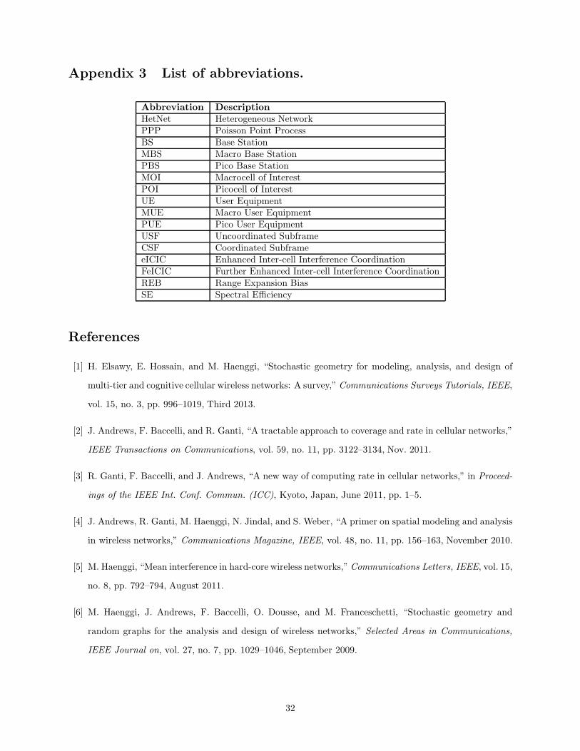
Appendix 3 List of abbreviations.

Abbreviation Description

HetNet Heterogeneous NetworkPPP Poisson Point ProcessBS Base StationMBS Macro Base StationPBS Pico Base StationMOI Macrocell of InterestPOI Picocell of InterestUE User EquipmentMUE Macro User EquipmentPUE Pico User EquipmentUSF Uncoordinated SubframeCSF Coordinated SubframeeICIC Enhanced Inter-cell Interference CoordinationFeICIC Further Enhanced Inter-cell Interference CoordinationREB Range Expansion BiasSE Spectral Efficiency

References

[1] H. Elsawy, E. Hossain, and M. Haenggi, “Stochastic geometry for modeling, analysis, and design of

multi-tier and cognitive cellular wireless networks: A survey,” Communications Surveys Tutorials, IEEE,

vol. 15, no. 3, pp. 996–1019, Third 2013.

[2] J. Andrews, F. Baccelli, and R. Ganti, “A tractable approach to coverage and rate in cellular networks,”

IEEE Transactions on Communications, vol. 59, no. 11, pp. 3122–3134, Nov. 2011.

[3] R. Ganti, F. Baccelli, and J. Andrews, “A new way of computing rate in cellular networks,” in Proceed-

ings of the IEEE Int. Conf. Commun. (ICC), Kyoto, Japan, June 2011, pp. 1–5.

[4] J. Andrews, R. Ganti, M. Haenggi, N. Jindal, and S. Weber, “A primer on spatial modeling and analysis

in wireless networks,” Communications Magazine, IEEE, vol. 48, no. 11, pp. 156–163, November 2010.

[5] M. Haenggi, “Mean interference in hard-core wireless networks,” Communications Letters, IEEE, vol. 15,

no. 8, pp. 792–794, August 2011.

[6] M. Haenggi, J. Andrews, F. Baccelli, O. Dousse, and M. Franceschetti, “Stochastic geometry and

random graphs for the analysis and design of wireless networks,” Selected Areas in Communications,

IEEE Journal on, vol. 27, no. 7, pp. 1029–1046, September 2009.

32

[7] S. Mukherjee, “Distribution of downlink SINR in heterogeneous cellular networks,” IEEE J. Select.

Areas Commun. (JSAC), Special Issue on Femtocell Networks, vol. 30, no. 3, pp. 575–585, Apr. 2012.

[8] R. Heath, M. Kountouris, and T. Bai, “Modeling heterogeneous network interference using poisson

point processes,” IEEE Trans. Signal Process., vol. 61, no. 16, pp. 4114–4126, Aug. 2013.

[9] T. Novlan, R. Ganti, and J. Andrews, “Coverage in two-tier cellular networks with fractional frequency

reuse,” in Proceedings of the IEEE Global Telecommun. Conf. (GLOBECOM), Houston, TX, Dec. 2011,

pp. 1–5.

[10] H. S. Dhillon, R. K. Ganti, F. Baccelli, and J. G. Andrews, “Modeling and analysis of K-tier downlink

heterogeneous cellular networks,” IEEE J. Select. Areas Commun. (JSAC), Special Issue on Femtocell

Networks, vol. 30, no. 3, pp. 550–560, Apr. 2012.

[11] S. Mukherjee, “Downlink SINR distribution in a heterogeneous cellular wireless network with biased

cell association,” in Proceedings of the IEEE Int. Conf. Commun. (ICC), Ottawa, Canada, June 2012,

pp. 6780 –6786.

[12] H.-S. Jo, Y. J. Sang, P. Xia, and J. Andrews, “Outage probability for heterogeneous cellular networks

with biased cell association,” in Proceedings of the IEEE Global Telecommun. Conf. (GLOBECOM),

Houston, TX, Dec. 2011, pp. 1–5.

[13] C.-H. Lee, C.-Y. Shih, and Y.-S. Chen, “Stochastic geometry based models for modeling cellular

networks in urban areas,” Springer Wireless Networks, vol. 19, no. 6, pp. 1063–1072, 2013. [Online].

Available: http://dx.doi.org/10.1007/s11276-012-0518-0

[14] OpenCellID website. [Online]. Available: www.opencellid.org

[15] D. Lopez-Perez, I. Guvenc, G. de la Roche, M. Kountouris, T. Q. Quek, and J. Zhang, “Enhanced inter-

cell interference coordination challenges in heterogeneous networks,” IEEE Wireless Commun. Mag.,

vol. 18, no. 3, pp. 22–31, June 2011.

[16] S. Singh and J. G. Andrews, “Joint resource partitioning and offloading in heterogeneous cellular net-

works,” CoRR, vol. abs/1303.7039, 2013.

[17] S. Singh, H. S. Dhillon, and J. G. Andrews, “Offloading in heterogeneous networks: Modeling, analysis,

and design insights,” IEEE Trans. Wireless Commun., vol. 12, no. 5, pp. 2484–2497, May 2013.

33

[18] S. Mukherjee and I. Guvenc, “Effects of range expansion and interference coordination on capacity and

fairness in heterogeneous networks,” in Proceedings of the IEEE Asilomar Conf. Sig., Syst., Computers,

vol. 1, Monterey, CA, Nov. 2011, pp. 1855–1859.

[19] A. Merwaday, S. Mukherjee, and I. Guvenc, “On the capacity analysis of hetnets with range expansion

and eICIC,” in Proceedings of the IEEE Global Commun. Conf. (GLOBECOM), Atlanta, GA, Dec 2013.

[20] Panasonic, “Performance study on ABS with reduced macro power,” 3GPP TSG-RAN WG1, Tech.

Rep. R1-113806, Nov. 2011.

[21] A. Morimoto, N. Miki, and Y. Okumura, “Investigation of inter-cell interference coordination applying

transmission power reduction in heterogeneous networks for LTE-advanced downlink,” IEICE Trans.

on Commun., vol. E96-B, no. 6, pp. 1327–1337, June 2013.

[22] M. Al-Rawi, J. Huschke, and M. Sedra, “Dynamic protected-subframe density configuration in LTE

heterogeneous networks,” in Proceedings of the IEEE Int. Conf. Computer Commun. Net. (ICCCN),

Munich, Germany, 2012, pp. 1–6.

[23] “Overview of 3gpp release 11 v0.1.7,” Dec. 2013. [Online]. Available:

http://www.3gpp.org/ftp/Information/WORK PLAN/Description Releases/Rel-11 description 20131224.zip

[24] Mpact lab data management. [Online]. Available: http://www.mpact.fiu.edu/data-management/

[25] Sitefinder website. [Online]. Available: http://www.sitefinder.ofcom.org.uk

[26] S. Mukherjee, “UE coverage in LTE macro network with mixed CSG and open access femto overlay,”

in Proceedings of the IEEE Int. Conf. Commun. (ICC) Workshops, Kyoto, Japan, June 2011, pp. 1–6.

[27] S. M. Yu and S.-L. Kim, “Downlink capacity and base station density in cellular networks,” in Proceed-

ings of the IEEE SpaSWiN workshop (in conjunction with WiOpt), Tsukuba Science City, Japan, May

2013, pp. 119–124.

[28] P. Viswanath, D. Tse, and R. Laroia, “Opportunistic beamforming using dumb antennas,” IEEE Trans.

Inf. Theory, vol. 48, no. 6, pp. 1277–1294, Aug. 2002.

[29] M. R. Jeong and N. Miki, “A comparative study on scheduling restriction schemes for lte-advanced net-

works,” in Proceedings of the IEEE 23rd Int. Symp. Personal Indoor and Mobile Radio Communications

(PIMRC), Sydney, Australia, Sept. 2012, pp. 488–495.

34