Capability Analysis - Minitab · CAPABILITY ANALYSIS 2 Data checks Stability To accurately estimate...
47
WWW.MINITAB.COM MINITAB ASSISTANT WHITE PAPER This paper explains the research conducted by Minitab statisticians to develop the methods and data checks used in the Assistant in Minitab Statistical Software. Capability Analysis Overview Capability analysis is used to evaluate whether a process is capable of producing output that meets customer requirements. The Minitab Assistant includes two capability analyses to examine continuous process data. Capability Analysis: This analysis evaluates capability based on a single process variable. Before/After Capability Comparison: This analysis evaluates whether an improvement effort made the process more capable of meeting customer requirements, by examining a single process variable before and after the improvement. To adequately estimate the capability of the current process and to reliably predict the capability of the process in the future, the data for these analyses should come from a stable process (Bothe, 1991; Kotz and Johnson, 2002). In addition, because these analyses estimate the capability statistics based on the normal distribution, the process data should follow a normal or approximately normal distribution. Finally, there should be enough data to ensure that the capability statistics have good precision and that the stability of the process can be adequately evaluated. Based on these requirements, the Assistant automatically performs the following checks on your data and displays the results in the Report Card: Stability Normality Amount of data In this paper, we investigate how these requirements relate to capability analysis in practice and describe how we established our guidelines to check for these conditions.
Transcript of Capability Analysis - Minitab · CAPABILITY ANALYSIS 2 Data checks Stability To accurately estimate...

WWW.MINITAB.COM
MINITAB ASSISTANT WHITE PAPER
This paper explains the research conducted by Minitab statisticians to develop the methods and
data checks used in the Assistant in Minitab Statistical Software.
Capability Analysis
Overview Capability analysis is used to evaluate whether a process is capable of producing output that
meets customer requirements. The Minitab Assistant includes two capability analyses to examine
continuous process data.
Capability Analysis: This analysis evaluates capability based on a single process variable.
Before/After Capability Comparison: This analysis evaluates whether an improvement
effort made the process more capable of meeting customer requirements, by examining
a single process variable before and after the improvement.
To adequately estimate the capability of the current process and to reliably predict the capability
of the process in the future, the data for these analyses should come from a stable process
(Bothe, 1991; Kotz and Johnson, 2002). In addition, because these analyses estimate the
capability statistics based on the normal distribution, the process data should follow a normal or
approximately normal distribution. Finally, there should be enough data to ensure that the
capability statistics have good precision and that the stability of the process can be adequately
evaluated.
Based on these requirements, the Assistant automatically performs the following checks on your
data and displays the results in the Report Card:
Stability
Normality
Amount of data
In this paper, we investigate how these requirements relate to capability analysis in practice and
describe how we established our guidelines to check for these conditions.

CAPABILITY ANALYSIS 2
Data checks
Stability To accurately estimate process capability, your data should come from a stable process. You
should verify the stability of your process before you check whether the data is normal and
before you evaluate the capability of the process. If the process is not stable, you should identify
and eliminate the causes of the instability.
Eight tests can be performed on variables control charts (Xbar-R/S or I-MR chart) to evaluate the
stability of a process with continuous data. Using these tests simultaneously increases the
sensitivity of the control chart. However, it is important to determine the purpose and added
value of each test because the false alarm rate increases as more tests are added to the control
chart.
Objective
We wanted to determine which of the eight tests for stability to include with the variables
control charts in the Assistant. Our first goal was to identify the tests that significantly increase
sensitivity to out-of-control conditions without significantly increasing the false alarm rate. Our
second goal was to ensure the simplicity and practicality of the chart. Our research focused on
the tests for the Xbar chart and the I chart. For the R, S, and MR charts, we use only test 1, which
signals when a point falls outside of the control limits.
Method
We performed simulations and reviewed the literature to evaluate how using a combination of
tests for stability affects the sensitivity and the false alarm rate of the control charts. In addition,
we evaluated the prevalence of special causes associated with the test. For details on the
methods used for each test, see the Results section below and Appendix B.
Results
We found that Tests 1, 2, and 7 were the most useful for evaluating the stability of the Xbar
chart and the I chart:
TEST 1: IDENTIFIES POINTS OUTSIDE OF THE CONTROL LIMITS
Test 1 identifies points > 3 standard deviations from the center line. Test 1 is universally
recognized as necessary for detecting out-of-control situations. It has a false alarm rate of only
0.27%.
TEST 2: IDENTIFIES SHIFTS IN THE MEANS
Test 2 signals when 9 points in a row fall on the same side of the center line. We performed a
simulation using 4 different means, set to multiples of the standard deviation, and determined
CAPABILITY ANALYSIS 3
the number of subgroups needed to detect a signal. We set the control limits based on the
normal distribution. We found that adding test 2 significantly increases the sensitivity of the
chart to detect small shifts in the mean. When test 1 and test 2 are used together, significantly
fewer subgroups are needed to detect a small shift in the mean than are needed when test 1 is
used alone. Therefore, adding test 2 helps to detect common out-of-control situations and
increases sensitivity enough to warrant a slight increase in the false alarm rate.
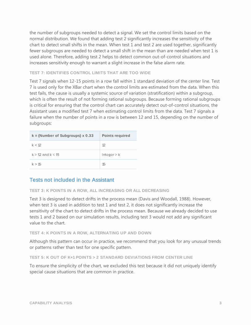
TEST 7: IDENTIFIES CONTROL LIMITS THAT ARE TOO WIDE
Test 7 signals when 12-15 points in a row fall within 1 standard deviation of the center line. Test
7 is used only for the XBar chart when the control limits are estimated from the data. When this
test fails, the cause is usually a systemic source of variation (stratification) within a subgroup,
which is often the result of not forming rational subgroups. Because forming rational subgroups
is critical for ensuring that the control chart can accurately detect out-of-control situations, the
Assistant uses a modified test 7 when estimating control limits from the data. Test 7 signals a
failure when the number of points in a row is between 12 and 15, depending on the number of
subgroups:
k = (Number of Subgroups) x 0.33 Points required
k < 12 12
k > 15 15
Tests not included in the Assistant
TEST 3: K POINTS IN A ROW, ALL INCREASING OR ALL DECREASING
Test 3 is designed to detect drifts in the process mean (Davis and Woodall, 1988). However,
when test 3 is used in addition to test 1 and test 2, it does not significantly increase the
sensitivity of the chart to detect drifts in the process mean. Because we already decided to use
tests 1 and 2 based on our simulation results, including test 3 would not add any significant
value to the chart.
TEST 4: K POINTS IN A ROW, ALTERNATING UP AND DOWN
Although this pattern can occur in practice, we recommend that you look for any unusual trends
or patterns rather than test for one specific pattern.
TEST 5: K OUT OF K+1 POINTS > 2 STANDARD DEVIATIONS FROM CENTER LINE
To ensure the simplicity of the chart, we excluded this test because it did not uniquely identify
special cause situations that are common in practice.

CAPABILITY ANALYSIS 4
TEST 6: K OUT OF K+1 POINTS > 1 STANDARD DEVIATION FROM THE CENTER LINE
To ensure the simplicity of the chart, we excluded this test because it did not uniquely identify
special cause situations that are common in practice.
TEST 8: K POINTS IN A ROW > 1 STANDARD DEVIATION FROM CENTER LINE (EITHER SIDE)
To ensure the simplicity of the chart, we excluded this test because it did not uniquely identify
special cause situations that are common in practice.
When checking stability in the Report Card, the Assistant displays the following status indicators:
Status Condition
No test failures on the chart for the mean (I chart or Xbar chart) and the chart for variation (MR, R, or S chart). The tests used for each chart are:
I chart: Test 1 and Test 2.
Xbar chart: Test 1, Test 2 and Test 7. Test 7 is only performed when control limits are estimated from the data.
MR, R and S charts: Test 1.
If above condition does not hold.
The specific messages that accompany each status condition are phrased in the context of
capability analysis; therefore, these messages differ from those used when the variables control
charts are displayed separately in the Assistant.
Normality In normal capability analysis, a normal distribution is fit to the process data and the capability
statistics are estimated from the fitted normal distribution. If the distribution of the process data
is not close to normal, these estimates may be inaccurate. The probability plot and the
Anderson-Darling (AD) goodness-of-fit test can be used to evaluate whether data are normal.
The AD test tends to have higher power than other tests for normality. The test can also more
effectively detect departures from normality in the lower and higher ends (tails) of a distribution
(D’Agostino and Stephens, 1986). These properties make the AD test well-suited for testing the
goodness-of-fit of the data when estimating the probability that measurements are outside the
specification limits.
Objective
Some practitioners have questioned whether the AD test is too conservative and rejects the
normality assumption too often when the sample size is extremely large. However, we could not
find any literature that discussed this concern. Therefore, we investigated the effect of large
sample sizes on the performance of the AD test for normality.

CAPABILITY ANALYSIS 5
We wanted to find out how closely the actual AD test results matched the targeted level of
significance (alpha, or Type I error rate) for the test; that is, whether the AD test incorrectly
rejected the null hypothesis of normality more often than expected when the sample size was
large. We also wanted to evaluate the power of the test to identify nonnormal distributions; that
is, whether the AD test correctly rejected the null hypothesis of normality as often as expected
when the sample size was large.
Method
We performed two sets of simulations to estimate the Type I error and the power of the AD test.
TYPE I ERROR: THE PROBABILITY OF REJECTING NORMALITY WHEN THE DATA ARE FROM A NORMAL DISTRIBUTION
To estimate the Type I error rate, we first generated 5000 samples of the same size from a
normal distribution. We performed the AD test for normality on every sample and calculated the
p-value. We then determined the value of k, the number of samples with a p-value that was less
than or equal to the significance level. The Type I error rate can then be calculated as k/5000. If
the AD test performs well, the estimated Type I error should be very close to the targeted
significance level.
POWER: THE PROBABILITY OF REJECTING NORMALITY WHEN THE DATA ARE NOT FROM A NORMAL DISTRIBUTION
To estimate the power, we first generated 5000 samples of the same size from a nonnormal
distribution. We performed the AD test for normality on every sample and calculated the p-
value. We then determined the value of k, the number of samples with a p-value that was less
than or equal to the significance level. The power can then be calculated as k/5000. If the AD
test performs well, the estimated power should be close to 100%.
We repeated this procedure for samples of different sizes and for different normal and
nonnormal populations. For more details on the methods and results, see Appendix B.
Results
TYPE I ERROR
Our simulations showed that when the sample size is large, the AD test does not reject the null
hypothesis more frequently than expected. The probability of rejecting the null hypothesis when
the samples are from a normal distribution (the Type I error rate) is approximately equal to the
target significance level, such as 0.05 or 0.1, even for sample sizes as large as 10,000.
POWER
Our simulations also showed that for most nonnormal distributions, the AD test has a power
close to 1 (100%) to correctly reject the null hypothesis of normality. The power of the test was
low only when the data were from a nonnormal distribution that was extremely close to a
CAPABILITY ANALYSIS 6
normal distribution. However, for these near normal distributions, a normal distribution is likely
to provide a good approximation for the capability estimates.
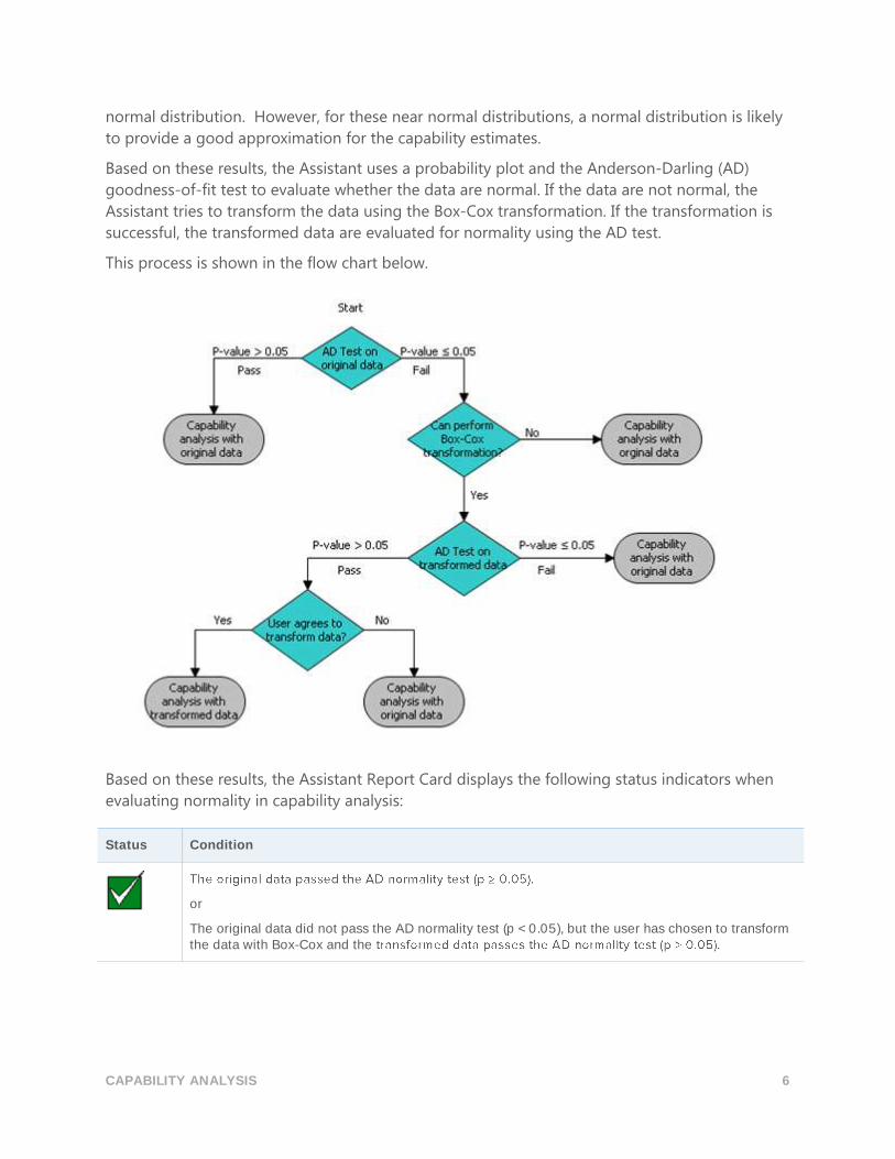
Based on these results, the Assistant uses a probability plot and the Anderson-Darling (AD)
goodness-of-fit test to evaluate whether the data are normal. If the data are not normal, the
Assistant tries to transform the data using the Box-Cox transformation. If the transformation is
successful, the transformed data are evaluated for normality using the AD test.
This process is shown in the flow chart below.
Based on these results, the Assistant Report Card displays the following status indicators when
evaluating normality in capability analysis:
Status Condition
or
The original data did not pass the AD normality test (p < 0.05), but the user has chosen to transform the data with Box-Cox and the

CAPABILITY ANALYSIS 7
Status Condition
The original data did not pass the AD normality test (p < 0.05). The Box-Cox transformation corrects the problem, but the user has chosen not to transform the data.
or
The original data did not pass the AD normality test (p < 0.05). The Box-Cox transformation cannot be successfully performed on the data to correct the problem.
Amount of data To obtain precise capability estimates, you need to have enough data. If the amount of data is
insufficient, the capability estimates may be far from the “true” values due to sampling
variability. To improve precision of the estimate, you can increase the number of observations.
However, collecting more observations requires more time and resources. Therefore, it is
important to know how the number of observations affects the precision of the estimates, and
how much data is reasonable to collect based on your available resources.
Objective
We investigated the number of observations that are needed to obtain precise estimates for
normal capability analysis. Our objective was to evaluate the effect of the number of
observations on the precision of the capability estimates and to provide guidelines on the
required amount of data for users to consider.
Method
We reviewed the literature to find out how much data is generally considered adequate for
estimating process capability. In addition, we performed simulations to explore the effect of the
number of observations on a key process capability estimate, the process benchmark Z. We
generated 10,000 normal data sets, calculated Z bench values for each sample, and used the
results to estimate the number of observations needed to ensure that the difference between
the estimated Z and the true Z falls within a certain range of precision, with 90% and 95%
confidence. For more details, see Appendix C.
Results
The Statistical Process Control (SPC) manual recommends using enough subgroups to ensure
that the major sources of process variation are reflected in the data (AIAG, 1995). In general,
they recommend collecting at least 25 subgroups, and at least 100 total observations. Other
sources cite an “absolute minimum” of 30 observations (Bothe, 1997), with a preferred minimum
of 100 observations.
Our simulation showed that the number of observations that are needed for capability estimates
depends on the true capability of the process and the degree of precision that you want your
estimate to have. For common target Benchmark Z values (Z >3), 100 observations provide 90%
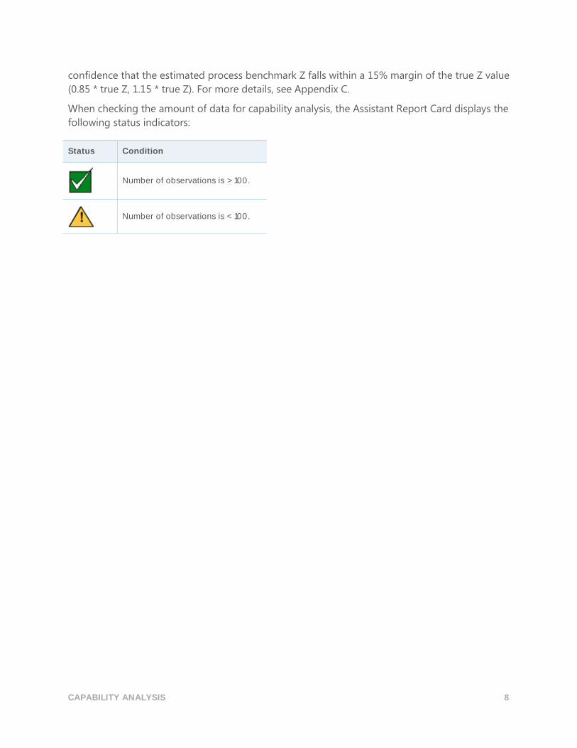
CAPABILITY ANALYSIS 8
confidence that the estimated process benchmark Z falls within a 15% margin of the true Z value
(0.85 * true Z, 1.15 * true Z). For more details, see Appendix C.
When checking the amount of data for capability analysis, the Assistant Report Card displays the
following status indicators:
Status Condition
Number of observations is > 100.
Number of observations is < 100.

CAPABILITY ANALYSIS 9
References AIAG (1995). Statistical process control (SPC) reference manual. Automotive Industry Action
Group.
Bothe, D.R. (1997). Measuring process capability: Techniques and calculations for quality and
manufacturing engineers. New York: McGraw-Hill.
D’Agostino, R.B., & Stephens, M.A. (1986). Goodness-of-fit techniques. New York: Marcel Dekker.
Kotz, S., & Johnson, N.L. (2002). Process capability indices – a review, 1992 – 2000. Journal of
Quality Technology, 34 (January), 2-53.
CAPABILITY ANALYSIS 10
Appendix A: Stability
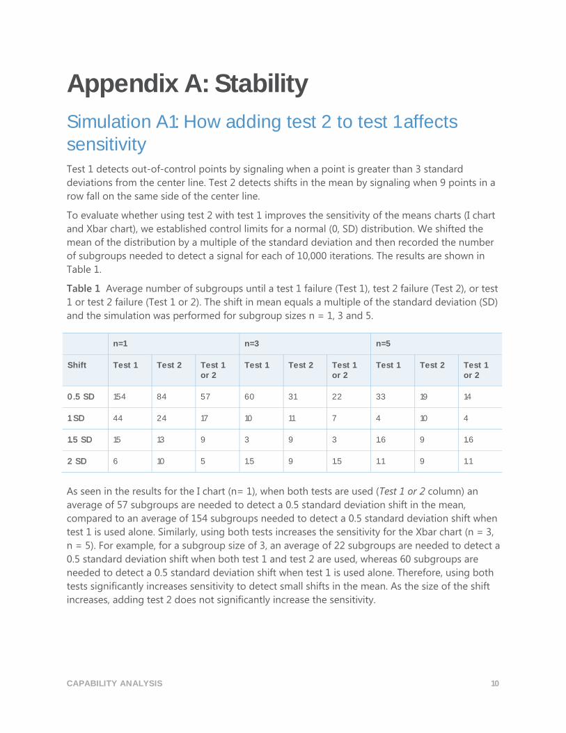
Simulation A1: How adding test 2 to test 1 affects sensitivity Test 1 detects out-of-control points by signaling when a point is greater than 3 standard
deviations from the center line. Test 2 detects shifts in the mean by signaling when 9 points in a
row fall on the same side of the center line.
To evaluate whether using test 2 with test 1 improves the sensitivity of the means charts (I chart
and Xbar chart), we established control limits for a normal (0, SD) distribution. We shifted the
mean of the distribution by a multiple of the standard deviation and then recorded the number
of subgroups needed to detect a signal for each of 10,000 iterations. The results are shown in
Table 1.
Table 1 Average number of subgroups until a test 1 failure (Test 1), test 2 failure (Test 2), or test
1 or test 2 failure (Test 1 or 2). The shift in mean equals a multiple of the standard deviation (SD)
and the simulation was performed for subgroup sizes n = 1, 3 and 5.
n=1 n=3 n=5
Shift Test 1 Test 2 Test 1 or 2
Test 1 Test 2 Test 1 or 2
Test 1 Test 2 Test 1 or 2
0.5 SD 154 84 57 60 31 22 33 19 14
1 SD 44 24 17 10 11 7 4 10 4
1.5 SD 15 13 9 3 9 3 1.6 9 1.6
2 SD 6 10 5 1.5 9 1.5 1.1 9 1.1
As seen in the results for the I chart (n= 1), when both tests are used (Test 1 or 2 column) an
average of 57 subgroups are needed to detect a 0.5 standard deviation shift in the mean,
compared to an average of 154 subgroups needed to detect a 0.5 standard deviation shift when
test 1 is used alone. Similarly, using both tests increases the sensitivity for the Xbar chart (n = 3,
n = 5). For example, for a subgroup size of 3, an average of 22 subgroups are needed to detect a
0.5 standard deviation shift when both test 1 and test 2 are used, whereas 60 subgroups are
needed to detect a 0.5 standard deviation shift when test 1 is used alone. Therefore, using both
tests significantly increases sensitivity to detect small shifts in the mean. As the size of the shift
increases, adding test 2 does not significantly increase the sensitivity.

CAPABILITY ANALYSIS 11
Simulation B2: How effectively does Test 7 detect stratification (multiple sources of variability in subgroups)? Test 7 typically signals a failure when between 12 and 15 points in a row fall within one standard
deviation of the center line. The Assistant uses a modified rule that adjusts the number of points
required based on the number of subgroups in the data. We set k = (number of subgroups *
0.33) and define the points in a row required for a test 7 failure as shown in Table 2.
Table 2 Points in a row required for a failure on test 7
k = (Number of Subgroups) x 0.33 Points required
k < 12 12
k > 15 15
Using common scenarios for setting control limits, we performed a simulation to determine the
likelihood that test 7 will signal a failure using the above criteria. Specifically, we wanted to
evaluate the rule for detecting stratification during the phase when control limits are estimated
from the data.
We randomly chose m subgroups of size n from a normal distribution with a standard deviation
(SD). Half of the points in each subgroup had a mean equal to 0 and the other half had a mean
equal to the SD shift (0 SD, 1 SD, or 2 SD). We performed 10,000 iterations and recorded the
percentage of charts that showed at least one test 7 failure, as shown in Table 3.
Table 3 Percentage of charts that have at least one signal from Test 7
Number of subgroups
Subgroup size
Test
m = 50
n = 2
15 in a row
m = 75
n = 2
15 in a row
m = 25
n = 4
12 in a row
m = 38
n = 4
13 in a row
m = 25
n = 6
12 in a row
Shift
0 SD 5% 8% 7% 8% 7%
1 SD 23% 33% 17% 20% 15%
2 SD 83% 94% 56% 66% 50%
As seen in the first Shift row of the table (shift = 0 SD), when there is no stratification, a relatively
small percentage of charts have at least one test 7 failure. However, when there is stratification
(shift = 1 SD or shift = 2 SD), a much higher percentage of charts—as many as 94%—have at

CAPABILITY ANALYSIS 12
least one test 7 failure. In this way, test 7 can identify stratification in the phase when the control
limits are estimated.

CAPABILITY ANALYSIS 13
Appendix B: Normality
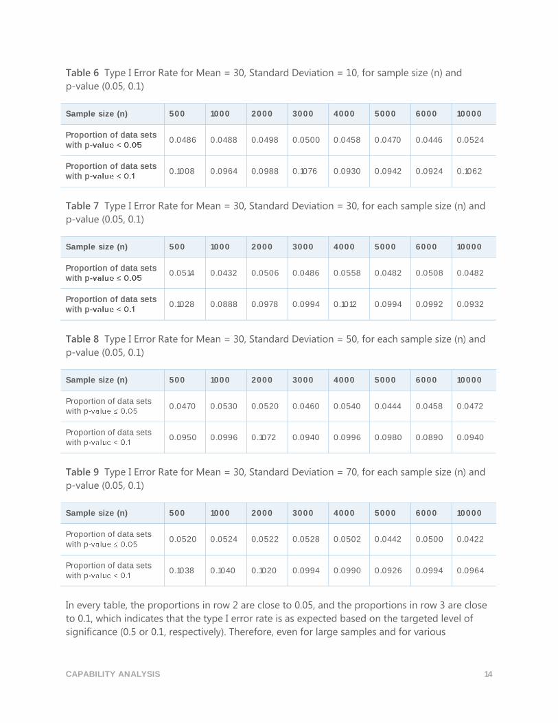
Simulation B.1: Estimating Type I error rate for the AD test To investigate the Type I error rate of the AD test for large samples, we generated different
dispersions of the normal distribution with a mean of 30 and standard deviations of 0.1, 5, 10,
30, 50 and 70. For each mean and standard deviation, we generated 5000 samples with sample
size n = 500, 1000, 2000, 3000, 4000, 5000, 6000, and 10000, respectively, and calculated the p-
value of the AD statistic. We then estimated the probabilities of rejecting normal distribution
given a normal data set by the proportion of the p-values ≤ 0.05, and ≤ 0.1 out of the 5000
samples. The results are shown in Tables 4-9 below.
Table 4 Type I Error Rate for Mean = 30, Standard Deviation = 0.1, for each sample size (n) and
p-value (0.05, 0.1)
Sample size (n) 500 1000 2000 3000 4000 5000 6000 10000
Proportion of data sets with p-0.05
0.0514 0.0480 0.0526 0.0458 0.0492 0.0518 0.0582 0.0486
Proportion of data sets with p-
0.1008 0.1008 0.0984 0.0958 0.1004 0.1028 0.1046 0.0960
Table 5 Type I Error Rate for Mean = 30, Standard Deviation = 5, for each sample size (n) and p-
value (0.05, 0.1)
Sample size (n) 500 1000 2000 3000 4000 5000 6000 10000
Proportion of data sets with p-0.05
0.0524 0.0520 0.0446 0.0532 0.0481 0.0518 0.0594 0.0514
Proportion of data sets with p-
0.0990 0.1002 0.0990 0.1050 0.0965 0.1012 0.1074 0.1030
CAPABILITY ANALYSIS 14
Table 6 Type I Error Rate for Mean = 30, Standard Deviation = 10, for sample size (n) and
p-value (0.05, 0.1)
Sample size (n) 500 1000 2000 3000 4000 5000 6000 10000
Proportion of data sets with p-
0.0486 0.0488 0.0498 0.0500 0.0458 0.0470 0.0446 0.0524
Proportion of data sets with p-
0.1008 0.0964 0.0988 0.1076 0.0930 0.0942 0.0924 0.1062
Table 7 Type I Error Rate for Mean = 30, Standard Deviation = 30, for each sample size (n) and
p-value (0.05, 0.1)
Sample size (n) 500 1000 2000 3000 4000 5000 6000 10000
Proportion of data sets with p-
0.0514 0.0432 0.0506 0.0486 0.0558 0.0482 0.0508 0.0482
Proportion of data sets with p-
0.1028 0.0888 0.0978 0.0994 0.1012 0.0994 0.0992 0.0932
Table 8 Type I Error Rate for Mean = 30, Standard Deviation = 50, for each sample size (n) and
p-value (0.05, 0.1)
Sample size (n) 500 1000 2000 3000 4000 5000 6000 10000
Proportion of data sets with p-
0.0470 0.0530 0.0520 0.0460 0.0540 0.0444 0.0458 0.0472
Proportion of data sets with p-
0.0950 0.0996 0.1072 0.0940 0.0996 0.0980 0.0890 0.0940
Table 9 Type I Error Rate for Mean = 30, Standard Deviation = 70, for each sample size (n) and
p-value (0.05, 0.1)
Sample size (n) 500 1000 2000 3000 4000 5000 6000 10000
Proportion of data sets with p-
0.0520 0.0524 0.0522 0.0528 0.0502 0.0442 0.0500 0.0422
Proportion of data sets with p-
0.1038 0.1040 0.1020 0.0994 0.0990 0.0926 0.0994 0.0964
In every table, the proportions in row 2 are close to 0.05, and the proportions in row 3 are close
to 0.1, which indicates that the type I error rate is as expected based on the targeted level of
significance (0.5 or 0.1, respectively). Therefore, even for large samples and for various

CAPABILITY ANALYSIS 15
dispersions of the normal distribution, the AD is not conservative but rejects the null hypothesis
as often as would be expected based on the targeted level of significance.
Simulation B.2: Estimating the power of the AD test To investigate the power of the AD test to detect nonnormality for large samples, we generated
data from many nonnormal distributions, including nonnormal distributions commonly used to
model process capability. For each distribution, we generated 5000 samples at each sample size
(n = 500, 1000, 3000, 5000, 7500, and 10000, respectively) and calculated the p-values for the
AD statistics. Then, we estimated the probability of rejecting the AD test for nonnormal data sets
by calculating the proportions of p-values ≤ 0.05, and p-values ≤ 0.1 out of the 5000 samples.
The results are shown in Tables 10-26 below.
Table 10 Power for t distribution with df = 3 for each sample size (n) and p-value (0.05, 0.1)
Sample size (n) 500 1000 2000 3000 4000 5000 7500 10000
Proportion of data sets with p-
1.00 1.00 1.00 1.00 1.00 1.00 1.00 1.00
Proportion of data sets with p-
1.00 1.00 1.00 1.00 1.00 1.00 1.00 1.00
Table 11 Power for t distribution with df = 5 for each sample size (n) and p-value (0.05, 0.1)
Sample size (n) 500 1000 2000 3000 4000 5000 7500 10000
Proportion of data sets with p-
0.9812 0.9998 1.00 1.00 1.00 1.00 0.9812 0.9998
Proportion of data sets with p-
0.9890 0.9998 1.00 1.00 1.00 1.00 0.9890 0.9998
Table 12 Power for Laplace (0,1) distribution for each sample size (n) and p-value (0.05, 0.1)
Sample size (n) 500 1000 2000 3000 4000 5000 7500 10000
Proportion of data sets with p-
1.00 1.00 1.00 1.00 1.00 1.00 1.00 1.00
Proportion of data sets with p-
1.00 1.00 1.00 1.00 1.00 1.00 1.00 1.00

CAPABILITY ANALYSIS 16
Table 13 Power for Uniform (0,1) distribution for each sample size (n) and p-value (0.05, 0.1)
Sample size (n) 500 1000 2000 3000 4000 5000 7500 10000
Proportion of data sets with p-
1.00 1.00 1.00 1.00 1.00 1.00 1.00 1.00
Proportion of data sets with p-
1.00 1.00 1.00 1.00 1.00 1.00 1.00 1.00
Table 14 Power for Beta (3,3) distribution for each sample size (n) and p-value (0.05, 0.1)
Sample size (n) 500 1000 2000 3000 4000 5000 7500 10000
Proportion of data sets with p-
0.7962 0.9944 1.00 1.00 1.00 1.00 0.7962 0.9944
Proportion of data sets with p-
0.8958 0.9944 1.00 1.00 1.00 1.00 0.8958 0.9944
Table 15 Power for Beta (8,1) distribution for each sample size (n) and p-value (0.05, 0.1)
Sample size (n) 500 1000 2000 3000 4000 5000 7500 10000
Proportion of data sets with p-
1.00 1.00 1.00 1.00 1.00 1.00 1.00 1.00
Proportion of data sets with p-
1.00 1.00 1.00 1.00 1.00 1.00 1.00 1.00
Table 16 Power for Beta (8,1) distribution for each sample size (n) and p-value (0.05, 0.1)
Sample size (n) 500 1000 2000 3000 4000 5000 7500 10000
Proportion of data sets with p-
1.00 1.00 1.00 1.00 1.00 1.00 1.00 1.00
Proportion of data sets with p-
1.00 1.00 1.00 1.00 1.00 1.00 1.00 1.00

CAPABILITY ANALYSIS 17
Table 17 Power for Expo (2) distribution for each sample size (n) and p-value (0.05, 0.1)
Sample size (n) 500 1000 2000 3000 4000 5000 7500 10000
Proportion of data sets with p-
1.00 1.00 1.00 1.00 1.00 1.00 1.00 1.00
Proportion of data sets with p-
1.00 1.00 1.00 1.00 1.00 1.00 1.00 1.00
Table 18 Power for Chi-Square (3) distribution for each sample size (n) and p-value (0.05, 0.1)
Sample size (n) 500 1000 2000 3000 4000 5000 7500 10000
Proportion of data sets with p-
1.00 1.00 1.00 1.00 1.00 1.00 1.00 1.00
Proportion of data sets with p-
1.00 1.00 1.00 1.00 1.00 1.00 1.00 1.00
Table 19 Power for Chi-Square (5) distribution for each sample size (n) and p-value (0.05, 0.1)
Sample size (n) 500 1000 2000 3000 4000 5000 7500 10000
Proportion of data sets with p-
1.00 1.00 1.00 1.00 1.00 1.00 1.00 1.00
Proportion of data sets with p-
1.00 1.00 1.00 1.00 1.00 1.00 1.00 1.00
Table 20 Power for Chi-Square (10) distribution for each sample size (n) and p-value (0.05, 0.1)
Sample size (n) 500 1000 2000 3000 4000 5000 7500 10000
Proportion of data sets with p-
1.00 1.00 1.00 1.00 1.00 1.00 1.00 1.00
Proportion of data sets with p-
1.00 1.00 1.00 1.00 1.00 1.00 1.00 1.00

CAPABILITY ANALYSIS 18
Table 21 Power for Gamma (2, 6) distribution for each sample size (n) and p-value (0.05, 0.1)
Sample size (n) 500 1000 2000 3000 4000 5000 7500 10000
Proportion of data sets with p-
1.00 1.00 1.00 1.00 1.00 1.00 1.00 1.00
Proportion of data sets with p-
1.00 1.00 1.00 1.00 1.00 1.00 1.00 1.00
Table 22 Power for Gamma(5, 6) distribution for each sample size (n) and p-value (0.05, 0.1)
Sample size (n) 500 1000 2000 3000 4000 5000 7500 10000
Proportion of data sets with p-
1.00 1.00 1.00 1.00 1.00 1.00 1.00 1.00
Proportion of data sets with p-
1.00 1.00 1.00 1.00 1.00 1.00 1.00 1.00
Table 23 Power for Gamma(10, 6) distribution for each sample size (n) and p-value (0.05, 0.1)
Sample size (n) 500 1000 2000 3000 4000 5000 7500 10000
Proportion of data sets with p-
0.9970 1.00 1.00 1.00 1.00 1.00 0.9970 1.00
Proportion of data sets with p-
0.9988 1.00 1.00 1.00 1.00 1.00 0.9988 1.00
Table 24 Power for Weibull(1, 4) distribution for each sample size (n) and p-value (0.05, 0.1)
Sample size (n) 500 1000 2000 3000 4000 5000 7500 10000
Proportion of data sets with p-
1.00 1.00 1.00 1.00 1.00 1.00 1.00 1.00
Proportion of data sets with p-
1.00 1.00 1.00 1.00 1.00 1.00 1.00 1.00
CAPABILITY ANALYSIS 19
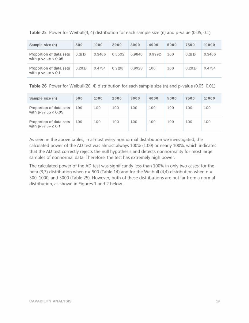
Table 25 Power for Weibull(4, 4) distribution for each sample size (n) and p-value (0.05, 0.1)
Sample size (n) 500 1000 2000 3000 4000 5000 7500 10000
Proportion of data sets with p-
0.1816 0.3406 0.8502 0.9840 0.9992 1.00 0.1816 0.3406
Proportion of data sets with p-
0.2818 0.4754 0.9198 0.9928 1.00 1.00 0.2818 0.4754
Table 26 Power for Weibull(20, 4) distribution for each sample size (n) and p-value (0.05, 0.01)
Sample size (n) 500 1000 2000 3000 4000 5000 7500 10000
Proportion of data sets with p-
1.00 1.00 1.00 1.00 1.00 1.00 1.00 1.00
Proportion of data sets with p-
1.00 1.00 1.00 1.00 1.00 1.00 1.00 1.00
As seen in the above tables, in almost every nonnormal distribution we investigated, the
calculated power of the AD test was almost always 100% (1.00) or nearly 100%, which indicates
that the AD test correctly rejects the null hypothesis and detects nonnormality for most large
samples of nonnormal data. Therefore, the test has extremely high power.
The calculated power of the AD test was significantly less than 100% in only two cases: for the
beta (3,3) distribution when n= 500 (Table 14) and for the Weibull (4,4) distribution when n =
500, 1000, and 3000 (Table 25). However, both of these distributions are not far from a normal
distribution, as shown in Figures 1 and 2 below.

CAPABILITY ANALYSIS 20
Figure 1 Comparison of the beta (3,3) distribution and a normal distribution.
As shown in Figure 1 above, the beta (3,3) distribution is close to a normal distribution. This
explains why there is a reduced proportion of data sets for which the null hypothesis of
normality is rejected by the AD test when the sample size is less than 1000.

CAPABILITY ANALYSIS 21
Figure 2 Comparison of the Weibull (4,4) distribution and a normal distribution.
Similarly, the Weibull (4,4) distribution is very close to a normal distribution, as shown in Figure
2. In fact, it is difficult to distinguish this distribution from a normal distribution. In this situation,
a normal distribution can be a good approximation to the true distribution, and the capability
estimates based on a normal distribution should provide a reasonable representation of the
process capability.

CAPABILITY ANALYSIS 22
Appendix C: Amount of data
Simulation C.1: Determining sample
sizes required for various levels of
precision
Setup and procedure
Without loss of generality, we generated samples using the following means and standard
deviations, assuming a lower spec limit (LSL) = -1 and an upper spec limit (USL) = 1:
Table 27 Mean, standard deviation, and target Z values for samples
Mean Standard deviation
Target Z
0 0.163 6.02
0.1 0.163 5.52
0.2 0.160 5.00
0.2 0.177 4.52
0 0.240 4.01
0.1 0.256 3.51
0.2 0.265 3.02
0.1 0.352 2.50
0 0.437 2.01
0 0.545 1.50
0.1 0.700 1.01

CAPABILITY ANALYSIS 23
We calculated the target Z values (the true Z) using the following formula, where μ is the mean
and σ is the standard deviation:
)/)(()(Pr1 LSLLSLXobp .
)./)(()/)((1)(Pr2 USLUSLUSLXobp
Target )()1( 21
1
21
1 ppppZ
To perform the simulation, we followed these steps:
1. Generate 10,000 normal data sets with a different sample size for each target Z (shown in
Table 27 above).
2. Calculate the Z bench values using the generated data sets. For each target Z and sample
size, there were 10,000 Z values.
3. Sort the 10,000 Z values from least to greatest. The 95% CI for Z bench was formed by
using the (250th, 9750th) estimated Z values; the 90% CI by using (500th, 9500th)
estimated Z values; and the 80% CI by using (1000th, 9000Th) estimated Z values.
4. Identify the number of observations that result in a difference between the estimated Z
and the true Z value within a certain range (precision) at the selected confidence levels.
To perform step 4 of the simulation, we first needed to determine the range, or level of
precision, that was appropriate to use in selecting the sample size. No single level of precision
can be successfully applied in all situations because the precision that is needed depends on the
true value of Z being estimated. For example, the table below shows the relationship between
fixed levels of precision and the defect per million opportunities (DPMO) for two different Z
values:
Table 28 Relationship between true Z, DPMO, and level of precision
True Z = 4.5, DPMO=3.4 True Z = 2.5, DPMO = 6209.7
Precision Lower DPMO Upper DPMO Lower DPMO Upper DPMO
True Z +/- 0.1 2.0 4.4 4661.2 8197.5
True Z +/- 0.2 1 8.5 3467.0 10724.1
True Z +/- 0.3 0.79 13.3 2555.0 13903.0
As shown in the table, if the Z value is 4.5, all three levels of precision (+/-0.1, +/0.2, and +/0.3 )
can be considered because in most applications the resulting difference in the values of the
lower DPMO and the upper DPMO, such as 0.79 vs. 13.3, may not make much practical
difference. However, if the true Z value is 2.5, the levels of precision +/-0.2 and +/-0.3 may not
be acceptable. For example, at the +/-0.3 level of precision, the upper DPMO is 13,903, which is

CAPABILITY ANALYSIS 24
substantially different from the lower DPMO value of 6209. Therefore, it seems that precision
should be chosen based on the true Z value.
For our simulation, we used the following three levels of precision to identify the number of
observations that are required.
Table 29 Levels of precision for Z for simulation
Margin Calculation Range of Z
15% True Z +/- 0.15 * True Z (0.85 True Z, 1.15 True Z)
10% True Z +/- 0.1 * True Z (0.9 True Z, 1.1 True Z)
5% True Z +/- 0.1 * True Z (0.95 True Z, 1.05 True Z)
SUMMARY OF RESULTS
The main results of the simulation are shown in table 30 below. The table shows the number of
observations required for different target Z values at each of the three levels of precision, with
90% confidence.
Table 30 Required number of observations for each precision margin at the 90% confidence
level
Number of observations
Target Z Target DPMO 15% Margin 10% Margin 5% Margin
6.02 0.00085 85 175 675
5.52 0.01695 85 175 650
5.00 0.28665 87 175 625
4.52 3.09198 90 175 600
4.01 30.36 83 175 650
3.51 224.1 90 185 650
3.02 1263.9 94 200 700
2.50 6209.7 103 215 750
2.01 22215.6 115 225 900
1.50 66807.2 135 300 1000
1.01 156247.6 185 400 1600

CAPABILITY ANALYSIS 25
Notice that as the margin of precision becomes narrower, the number of observations required
increases. In addition, if we increase the confidence level from 90% to 95%, substantially more
observations are needed, which is evident in the detailed simulation results shown in tables 31-
52 in the section below.
Based on the results of the simulation, we conclude that:
1. The number of observations required to produce reasonably precise capability estimates
varies with the true capability of the process.
2. For common target Benchmark Z values (Z >3), using a minimum of 100 observations,
you have approximately 90% confidence that your estimated process benchmark Z is
within 15% of the true Z value (0.85 * true Z, 1.15 * true Z). If you increase the number of
observations to 175 or more, the precision of the estimated benchmark Z falls within a
10% margin (0.9 * true Z, 1.1 * true Z).
DETAILED SIMULATION RESULTS
The following tables show the specific results of the simulation that were summarized in Table
30 above. For each target Z, and for each confidence level and each level of precision, we
identify the minimum number of observations such that the corresponding confidence interval
lies inside the referenced interval.
For example, in the first set of results shown below, when target Z = 6.02, the reference interval
for the 15% margin of precision is calculated to be (5.117, 6.923) as shown in row 1 of Table 31.
Note that in Table 32, at 90% confidence, the intervals in column 3 do not lie within this
reference interval until the number of observations increases to 85. Therefore, 85 is the
estimated minimum number of observations needed to achieve 90% confidence with a 15%
margin of precision when the target Z is 6.02. The results for the confidence levels and precision
margins for the other target Z values in tables 33-51 can be interpreted similarly.
TARGET Z= 6.02 TARGET DPMO = 0.00085
Table 31 Reference intervals used to select the minimum number of observations for each level
of precision
Precision Lower limit Upper Limit
15% margin Z 0.15Z = 5.117 Z + 0.15Z = 6.923
10% margin Z 0.1Z = 5.42 Z + 0.1Z = 6.62
5% margin Z 0.05Z = 5.72 Z + 0.05Z = 6.32

CAPABILITY ANALYSIS 26
Table 32 Simulated confidence intervals of the benchmark Z for various numbers of
observations
Number of observations
95% CI 90% CI 80% CI
5 (3.36, 20.97) (3.64, 13.91) (4.04, 11.22)
10 (3.97, 11.82) (4.23, 9.65) (4.54, 8.63)
15 (4.26, 10.14) (4.49, 8.65) (4.79, 7.95)
20 (4.47, 9.40) (4.67, 8.16) (4.93, 7.63)
25 (4.60, 8.82) (4.79, 7.87) (5.01, 7.43)
30 (4.70, 8.49) (4.88, 7.65) (5.10, 7.25)
35 (4.78, 8.23) (4.95, 7.52) (5.16, 7.12)
40 (4.86, 8.08) (5.02, 7.43) (5.22, 7.09)
45 (4.90, 7.89) (5.05, 7.30) (5.26, 7.00)
50 (4.94, 7.78) (5.09, 7.25) (5.28, 6.93)
60 (5.05, 7.55) (5.18, 7.08) (5.34, 6.81)
70 (5.11, 7.43) (5.24, 6.97) (5.39, 6.75)
80 (5.15, 7.32) (5.28, 6.94) (5.43, 6.71)
85 (5.30, 6.92)
90 (5.20, 7.23) (5.32, 6.87) (5.46, 6.67)
100 (5.24, 7.15) (5.35, 6.83) (5.48, 6.64)
105 (5.26, 7.13) (5.37, 6.81) (5.51, 6.63)
110 (5.27, 7.10) (5.38, 6.78) (5.51, 6.60)
120 (5.31, 7.07) (5.41, 6.73) (5.54, 6.55)
130 (5.34, 7.00) (5.44, 6.71) (5.56, 6.55)
140 (5.35, 6.97) (5.45, 6.70) (5.57, 6.54)
150 (5.37, 6.89) (5.47, 6.67) (5.58, 6.51)
175 (5.42, 6.87) (5.50, 6.62) (5.62, 6.48)
200 (5.46, 6.77) (5.54, 6.55) (5.64, 6.43)

CAPABILITY ANALYSIS 27
Number of observations
95% CI 90% CI 80% CI
250 (5.51, 6.71) (5.58, 6.51) (5.67, 6.40)
300 (5.56, 6.62) (5.63, 6.46) (5.71, 6.36)
350 (5.59, 6.59) (5.65, 6.43) (5.73, 6.34)
400 (5.62, 6.54) (5.68, 6.40) (5.75, 6.32)
450 (5.62, 6.51) (5.69, 6.38) (5.76, 6.30)
500 (5.65, 4.50) (5.71, 6.36) (5.78, 6.28)
550 (5.68, 6.46) (5.73, 6.35) (5/79, 6.27)
650 (5.71, 6.43) (5.75, 6.32) (5.81, 6.24)
700 (5.71, 6.41) (5.76, 6.31) (5.81, 6.24)
900 (5.75, 6.37) (5.79, 6.27) (5.84, 6.21)
1000 (5.76, 6.34) (5.80, 6.26) (5.85, 6.20)
1050 (5.77, 6.35) (5.81, 6.25) (5.85, 6.20)
1100 (5.77, 6.33) (5.81, 6.25) (5.86, 6.20)
1150 (5.78, 6.32) (5.82, 6.25) (5.86, 6.20)
1200 (5.78, 6.33) (5.82, 6.24) (5.86, 6.18)
1250 (5.79, 6.32) (5.82, 6.23) (5.87, 6.18)
1300 (5.80, 6.31) (5.83, 6.23) (5.87, 6.18)
1350 (5.80, 6.30) (5.83, 6.22) (5.87, 6.18)
1400 (5.80, 6.30) (5.83, 6.22) (5.88, 6.18)
1450 (5.80, 6.28) (5.84, 6.22) (5.88, 6.17)
1500 (5.81, 6.28) (5.84, 6.21) (5.88, 6.17)
1550 (5.81, 6.28) (5.84, 6.21) (5.88, 6.17)
1600 (5.81, 6.28) (5.85, 6.21) (5.88, 6.17)
1650 (5.81, 6.28) (5.85, 6.21) (5.89, 6.17)
1700 (5.81, 6.27) (5.85, 6.20) (5.89, 6.17)

CAPABILITY ANALYSIS 28
TARGET Z = 5.52 TARGET DPMO = 0.01695
Table 33 Reference intervals used to select the minimum number of observations for each level
of precision
Precision Lower limit Upper Limit
15% margin Z 0.15Z = 4.6920 Z + 0.15Z = 6.3480
10% margin Z 0.1Z = 4.97 Z + 0.1Z = 6.07
5% margin Z 0.05Z = 5.24 Z + 0.05Z = 5.80
Table 34 Simulated confidence intervals of the benchmark Z for various numbers of
observations
Number of observations
95% CI 90% CI 80% CI
5 (3.18, 18.68) (3.49, 12.87) (3.86, 10.62)
10 (3.68, 11.28) (3.92, 9.12) (4.22, 8.14)
15 (3.99, 9.38) (4.20, 8.03) (4.46, 7.40)
20 (4.15, 8.74) (4.34, 7.64) (4.59, 7.08)
25 (4.27, 8.18) (4.45, 7.32) (4.67, 6.86)
30 (4.36, 7.80) (4.52, 7.13) (4.75, 6.72)
35 (4.43, 7.61) (4.59, 6.94) (4.79, 6.60)
40 (4.47, 7.45) (4.64, 6.84) (4.82, 6.53)
45 (4.56, 7.23) (4.69, 6.73) (4.86, 6.44)
50 (4.55, 7.14) (4.71, 6.65) (4.88, 6.38)
60 (4.65, 7.00) (4.78, 6.56) (4.93, 6.32)
70 (4.71, 6.84) (4.82, 6.46) (4.97, 6.23)
80 (4.75, 6.73) (4.87, 6.38) (5.00, 6.18)
83 (4.88, 6.36)
84 (4.87, 6.37)
85 (4.89, 6.32)
90 (4.80, 6.65) (4.91, 6.33) (5.03, 6.14)

CAPABILITY ANALYSIS 29
Number of observations
95% CI 90% CI 80% CI
100 (4.84, 6.60) (4.94, 6.29) (5.06, 6.12)
115 (4.86, 6.50) (4.96, 6.23) (5.08, 6.07)
125 (4.88, 6.45) (4.99, 6.19) (5.10, 6.04)
150 (4.94, 6.38) (5.03, 6.13) (5.14, 5.99)
175 (4.98, 6.17) (5.06, 6.06) (5.16, 5.95)
200 (5.02, 6.21) (5.09, 6.03) (5.18, 5.92)
250 (5.06, 6.15) (5.14, 5.98) (5.22, 5.87)
300 (5.10, 6.09) (5.16, 5.94) (5.24, 5.84)
350 (5.13, 6.04) (5.19, 5.90) (5.26, 5.81)
375 (5.13, 6.02) (5.19, 5.88) (5.27, 5.80)
400 (5.15, 6.00) (5.21, 5.87) (5.28, 5.79)
450 (5.18, 5.98) (5.22, 5.85) (5.29, 5.78)
500 (5.19, 5.96) (5.24, 5.84) (5.30, 5.77)
650 (5.23, 5.83) (5.27, 5.80) (5.33, 5.73)
700 (5.24, 5.89) (5.28, 5.78) (5.34, 5.72)
800 (5.25, 5.86) (5.29, 5.76) (5.35, 5.71)
900 (5.27, 5.83) (5.31, 5.75) (5.36, 5.70)
1000 (5.28, 5.82) (5.32, 5.74) (5.37, 5.69)
1100 (5.29, 5.80) (5.33, 5.73) (5.37, 5.68)
1200 (5.30, 5.79) (5.33, 5.72) (5.38, 5.68)
1300 (5.31, 5.78) (5.34, 5.71) (5.38, 5.67)
1400 (5.31, 5.77) (5.35, 5.70) (5.39, 5.66)
1500 (5.32, 5.76) (5.35, 5.70) (5.39, 5.66)
1600 (5.33, 5.76) (5.36, 5.69) (5.40, 5.65)
1700 (5.34, 5.75) (5.37, 5.69) (5.40, 5.65)

CAPABILITY ANALYSIS 30
TARGET Z = 5.00 TARGET DPMO = 0.28665
Table 35 Reference intervals used to select the minimum number of observations for each level
of precision
Precision Lower limit Upper Limit
15% margin Z 0.15Z = 4.25 Z + 0.15Z = 5.75
10% margin Z 0.1Z = 4.5 Z + 0.1Z = 5.5
5% margin Z 0.05Z = 4.75 Z + 0.05Z = 5.25
Table 36 Simulated confidence intervals of the benchmark Z for various numbers of
observations
Number of observations
95% CI 90% CI 80% CI
10 (3.38, 10.10) (3.57, 8.23) (3.85, 7.36)
20 (3.74, 7.80) (3.93, 6.89) (4.16, 6.39)
30 (3.94, 7.16) (4.10, 6.47) (4.28, 6.11)
40 (4.07, 6.69) (4.20, 6.18) (4.35, 5.90)
50 (4.15, 6.48) (4.27, 6.06) (4.41, 5.80)
60 (4.20, 6.27) (4.32, 5.92) (4.45, 5.70)
70 (4.26, 6.23) (4.37, 5.86) (4.50, 5.64)
80 (4.29, 6.10) (4.40, 5.78) (4.53, 5.59)
87 (4.43, 5.75)
90 (4.31, 6.05) (4.43, 5.74) (4.55, 5.56)
100 (4.35, 5.96) (4.44, 5.68) (4.57, 5.53)
115 (4.40, 5.91) (4.49, 5.64) (4.60, 5.50)
125 (4.40, 5.84) (4.50, 5.60) (4.61, 5.46)
150 (4.47, 5.76) (4.55, 5.55) (4.65, 5.43)
170 (4.50, 5.70) (4.57, 5.51) (4.66, 5.39)
175 (4.50, 5.70) (4.58, 5.49) (4.67, 5.39)
200 (4.54, 5.65) (4.60, 5.48) (4.69, 5.37)

CAPABILITY ANALYSIS 31
Number of observations
95% CI 90% CI 80% CI
250 (4.58, 5.57) (4.64, 5.41) (4.73, 5.32)
300 (4.61, 5.52) (4.67, 5.38) (4.74, 5.29)
350 (4.64, 5.47) (4.70, 5.34) (4.76, 5.26)
400 (4.66, 5.45) (4.71, 5.32) (4.77, 5.25)
450 (4.68, 5.42) (4.73, 5.30) (4.79, 5.23)
500 (4.69, 5.39) (4.74, 5.29) (4.80, 5.23)
600 (4.73, 5.35) (4.77, 5.26) (4.82, 5.20)
625 (4.73, 5.36) (4.77, 5.25) (4.82, 5.20)
700 (4.74, 5.32) (4.78, 5.23) (4.83, 5.18)
800 (4.76, 5.31) (4.80, 5.23) (4.85, 5.17)
900 (4.77, 5.28) (4.81, 5.21) (4.85, 5.16)
1000 (4.78, 5.27) (4.82, 5.20) (4.86, 5.16)
1100 (4.79, 5.26) (4.82, 5.19) (4.86, 5.15)
1200 (4.80, 5.25) (4.83, 5.18) (4.87, 5.14)
1300 (4.81, 5.24) (4.83, 5.17) (4.87, 5.13)
1400 (4.82, 5.22) (4.84, 5.16) (4.88, 5.13)
1500 (4.83, 5.22) (4.85, 5.17) (4.88, 5.13)
1600 (4.82, 5.22) (4.85, 5.16) (4.88, 5.13)
1700 (4.83, 5.21) (4.86, 5.16) (4.89, 5.12)

CAPABILITY ANALYSIS 32
TARGET Z = 4.52 TARGET DPMO = 3.09198
Table 37 Reference intervals used to select the minimum number of observations for each level
of precision.
Precision Lower limit Upper limit
15% margin Z 0.15Z = 3.842 Z + 0.15Z = 5.198
10% margin Z 0.1Z = 4.07 Z + 0.1Z = 4.97
5% margin Z 0.05Z = 4.29 Z + 0.05Z = 4.75
Table 38 Simulated confidence intervals of the benchmark Z for various numbers of
observations
Number of observations
95% CI 90% CI 80% CI
10 (3.03, 9.22) (3.22, 7.50) (3.49, 6.72)
20 (3.36, 7.07) (3.51, 6.20) (3.72, 5.78)
30 (3.54, 6.45) (3.69, 5.83) (3.86, 5.52)
40 (3.64, 6.08) (3.78, 5.59) (3.94, 5.34)
50 (3.75, 5.87) (3.85, 5.46) (3.99, 5.23)
60 (3.80, 5.76) (3.91, 5.37) (4.04, 5.17)
70 (3.84, 5.61) (3.94, 5.28) (4.07, 5.10)
80 (3.88, 5.53) (3.98, 5.24) (4.09, 5.07)
90 (3.91, 5.47) (4.00, 5.20) (4.12, 5.04)
92 (4.00, 5.19)
100 (3.93, 5.40) (4.02, 5.15) (4.13, 5.01)
115 (3.96, 5.34) (4.05, 5.10) (4.16, 4.96)
150 (4.04, 5.23) (4.11, 5.03) (4.20, 4.91)
175 (4.07, 5.16) (4.14, 4.97) (4.22, 4.87)
200 (4.10, 5.12) (4.16, 4.95) (4.24, 4.85)
250 (4.14, 5.03) (4.20, 4.90) (4.27, 4.82)
300 (4.17, 4.99) (4.22, 4.86) (4.29, 4.79)
CAPABILITY ANALYSIS 33
Number of observations
95% CI 90% CI 80% CI
350 (4.20, 4.96) (4.25, 4.83) (4.30, 4.76)
400 (4.21, 4.93) (4.26, 4.81) (4.32, 4.75)
450 (4.23, 4.90) (4.27, 4.79) (4.32, 4.73)
500 (4.24, 4.88) (4.29, 4.78) (4.34, 4.72)
600 (4.27, 4.84) (4.31, 4.76) (4.35, 4.71)
700 (4.29, 4.82) (4.32, 4.74) (4.36, 4.69)
800 (4.29, 4.80) (4.33, 4.72) (4.37, 4.68)
900 (4.31, 4.78) (4.34, 4.71) (4.38, 4.67)
1000 (4.32, 4.76) (4.35, 4.70) (4.39, 4.66)
1100 (4.33, 4.75) (4.36, 4.68) (4.39, 4.65)
1200 (4.34, 4.74) (4.37, 4.68) (4.40, 4.65)
1300 (4.34, 4.74) (4.37, 4.68) (4.40, 4.64)
1400 (4.35, 4.74) (4.38, 4.67) (4.41, 4.64)
1500 (4.36, 4.72) (4.38, 4.67) (4.41, 4.63)
1600 (4.36, 4.72) (4.39, 4.66) (4.42, 4.63)
1700 (4.36, 4.71) (4.39, 4.66) (4.42, 4.63)
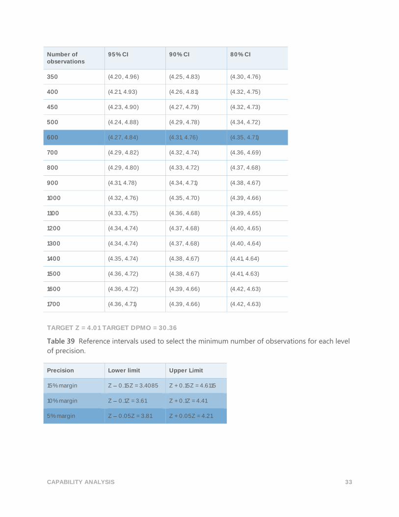
TARGET Z = 4.01 TARGET DPMO = 30.36
Table 39 Reference intervals used to select the minimum number of observations for each level
of precision.
Precision Lower limit Upper Limit
15% margin Z 0.15Z = 3.4085 Z + 0.15Z = 4.6115
10% margin Z 0.1Z = 3.61 Z + 0.1Z = 4.41
5% margin Z 0.05Z = 3.81 Z + 0.05Z = 4.21

CAPABILITY ANALYSIS 34
Table 40 Simulated confidence intervals of the benchmark Z for various numbers of
observations
Number of observations
95% CI 90% CI 80% CI
5 (2.12, 12.84) (2.32, 9.13) (2.61, 7.35)
10 (2.57, 7.96) (2.75, 6.50) (2.97, 5.79)
15 (2.79, 6.75) (2.95, 5.82) (3.13, 5.32)
20 (2.92, 6.21) (3.06, 5.46) (3.23, 5.08)
25 (2.99, 5.85) (3.12, 5.24) (3.29, 4.91)
30 (3.09, 5.63) (3.20, 5.08) (3.35, 4.83)
35 (3.13, 5.50) (3.26, 5.04) (3.40, 4.76)
40 (3.17, 5.38) (3.29, 4.95) (3.44, 4.71)
45 (3.22, 5.25) (3.33, 4.86) (3.47, 4.65)
50 (3.27, 5.15) (3.36, 4.82) (3.49, 4.62)
60 (3.32, 5.09) (3.42, 4.76) (3.53, 4.56)
70 (3.35, 4.98) (3.44, 4.68) (3.56, 4.52)
80 (3.41, 4.88) (3.50, 4.63) (3.60, 4.48)
83 (3.50, 4.61)
85 (3.50, 4.60)
90 (3.44, 4.82) (3.52, 4.58) (3.62, 4.44)
100 (3.47, 4.76) (3.55, 4.55) (3.64, 4.43)
110 (3.48, 4.76) (3.56, 4.51) (3.65, 4.40)
115 (3.48, 4.73) (3.56, 4.52) (3.66, 4.39)
150 (3.55, 4.63) (3.62, 4.44) (3.70, 4.33)
175 (3.58, 4.57) (3.65, 4.41) (3.72, 4.32)
200 (3.61, 4.53) (3.67, 4.38) (3.74, 4.29)
250 (3.65, 4.47) (3.70, 4.33) (3.77, 4.26)
300 (3.68, 4.43) (3.73, 4.31) (3.79, 4.24)

CAPABILITY ANALYSIS 35
Number of observations
95% CI 90% CI 80% CI
350 (3.70, 4.40) (3.74, 4.28) (3.80, 4.22)
400 (3.72, 4.36) (3.76, 4.27) (3.81, 4.20)
450 (3.74, 4.35) (3.78, 4.25) (3.82, 4.19)
500 (3.75, 4.33) (3.79, 4.24) (3.84, 4.18)
650 (3.78, 4.28) (3.81, 4.21) (3.86, 4.16)
675 (3.79, 4.27) (3.82, 4.20) (3.86, 4.16)
700 (3.78, 4.28) (3.82, 4.20) (3.86, 4.16)
900 (3.81, 4.25) (3.84, 4.18) (3.88, 4.14)
1000 (3.82, 4.23) (3.85, 4.16) (3.88, 4.13)
1100 (3.83, 4.22) (3.86, 4.16) (3.89, 4.12)
1200 (3.84, 4.21) (3.87, 4.15) (3.89, 4.12)
1300 (3.84, 4.20) (3.87, 4.15) (3.90. 4.12)
1400 (3.85, 4.19) (3.88, 4.14) (3.90, 4.11)
1500 (3.86, 4.18) (3.88, 4.14) (3.91, 4.11)
1600 (3.86, 4.18) (3.88, 4.13) (3.91, 4.10)
1700 (3.86, 4.18) (3.89, 4.13) (3.91, 4.10)
TARGET Z = 3.51 TARGET DPMO = 224.1
Table 41 Reference intervals used to select the minimum number of observations for each level
of precision
Precision Lower limit Upper Limit
15% margin Z 0.15Z =2.9835 Z + 0.15 Z = 4.0365
10% margin Z 0.1Z = 3.16 Z + 0.1Z = 3.86
5% margin Z 0.05Z = 3.33 Z + 0.05Z = 3.69

CAPABILITY ANALYSIS 36
Table 42 Simulated confidence intervals of the benchmark Z for various numbers of
observations
Number of observations
95% CI 90% CI 80% CI
10 (2.27, 7.08) (2.43, 5.80) (2.63, 5.17)
20 (2.57, 5.56) (2.68, 4.88) (2.85, 5.52)
30 (2.71, 5.05) (2.83, 4.54) (2.96, 4.28)
40 (2.80, 4.73) (2.90, 4.37) (3.02, 4.16)
50 (2.86, 4.57) (2.97, 4.25) (3.08, 4.07)
60 (2.92, 4.44) (3.00, 4.18) (3.10, 4.03)
70 (2.95, 4.37) (3.03, 4.13) (3.12, 3.98)
80 (2.97, 4.33) (3.06, 4.08) (3.15, 3.94)
90 (3.01, 4.26) (3.08, 4.04) (3.17, 3.90)
100 (3.03, 4.22) (3.11, 4.02) (3.19, 3.89)
110 (3.05, 4.16) (3.11, 3.98) (3.20, 3.86)
150 (3.12, 4.06) (3.17, 3.91) (3.24, 3.81)
175 (3.14, 4.02) (3.19, 3.87) (3.27, 3.79)
185 (3.14, 4.00) (3.20, 3.86) (3.26, 3.78)
200 (3.17, 3.97) (3.22, 3.84) (3.28, 3.77)
250 (3.20, 3.92) (3.24, 3.80) (3.30, 3.74)
300 (3.22, 3.88) (3.26, 3.78) (3.31, 3.72)
350 (3.24, 3.86) (3.29, 3.76) (3.33, 3.71)
400 (3.25, 3.83) (3.30, 3.75) (3.34, 3.69)
450 (3.27, 3.81) (3.31, 3.72) (3.35, 3.67)
500 (3.28, 3.79) (3.31, 3.71) (3.36, 3.67)
600 (3.30, 3.77) (3.33, 3.70) (3.37, 3.65)
650 (3.31, 3.76) (3.34, 3.69) (3.37, 3.65)
700 (3.31, 3.74) (3.34, 3.68) (3.38, 3.64)

CAPABILITY ANALYSIS 37
Number of observations
95% CI 90% CI 80% CI
800 (3.33, 3.74) (3.35, 3.67) (3.38, 3.63)
900 (3.33, 3.71) (3.36, 3.66) (3.39, 3.62)
1000 (3.34, 3.71) (3.37, 3.65) (3.40, 3.61)
1100 (3.35, 3.69) (3.38, 3.64) (3.40, 3.61)
1200 (3.36, 3.69) (3.38, 3.64) (3.41, 3.61)
1300 (3.36, 3.69) (3.39, 3.63) (3.41, 3.60)
1400 (3.37, 3.67) (3.39, 3.63) (3.42, 3.60)
1500 (3.38, 3.67) (3.40, 3.62) (3.42, 3.60)
1600 (3.38, 3.66) (3.40, 3.62) (3.42, 3.59)
1700 (3.38, 3.66) (3.40, 3.61) (3.42, 3.59)
TARGET Z = 3.02 TARGET DPMO = 1263.9
Table 43 Reference intervals used to select the minimum number of observations for each level
of precision
Precision Lower limit Upper limit
15% margin Z 0.15Z = 2.567 Z + 0.15Z = 3.473
10% margin Z 0.1Z = 2.72 Z + 0.1Z = 3.32
5% margin Z 0.05Z = 2.87 Z + 0.05Z = 3.17
Table 44 Simulated confidence intervals of the benchmark Z for various numbers of
observations
Number of observations
95% CI 90% CI 80% CI
10 (1.92, 6.26) (2.07, 5.02) (2.26, 4.49)
20 (2.22, 4.83) (2.33, 4.23) (2.46, 3.91)
30 (2.32, 4.34) (2.42, 3.92) (2.54, 3.70)
40 (2.40. 4.11) (2.48, 3.77) (2.60, 3.58)

CAPABILITY ANALYSIS 38
Number of observations
95% CI 90% CI 80% CI
50 (2.45, 3.96) (2.55, 3.68) (2.64, 3.52)
60 (2.50, 3.87) (2.58, 3.62) (2.68, 3.48)
70 (2.54, 3.79) (2.61, 3.55) (2.70, 3.43)
80 (2.56, 3.73) (2.63, 3.52) (2.71, 3.40)
90 (2.59, 3.68) (2.65, 3.49) (2.73, 3.38)
94 (2.66, 3.47)
100 (2.61, 3.65) (2.67, 3.46) (2.74, 3.36)
110 (2.62, 3.61) (2.69, 3.44) (2.76, 3.34)
120 (2.64, 3.58) (2.70, 3.42) (2.76, 3.32)
150 (2.68, 3.52) (2.73, 3.37) (2.79, 3.29)
200 (2.72, 3.44) (2.76, 3.32) (2.81, 3.25)
250 (2.75, 3.38) (2.79, 3.28) (2.84, 3.23)
300 (2.77, 3.36) (2.81, 3.26) (2.86, 3.20)
350 (2.78, 3.32) (2.82, 3.24) (2.87, 3.19)
400 (2.80, 3.30) (2.83, 3.22) (2.87, 3.18)
425 (2.81, 3.29) (2.84, 3.22) (2.88, 3.17)
450 (2.81, 3.28) (2.85, 3.21) (2.88, 3.17)
500 (2.82, 3.28) (2.85, 3.20) (2.88, 3.16)
600 (2.84, 3.25) (2.87, 3.19) (2.90, 3.15)
650 (2.84, 3.24) (2.87, 3.18) (2.90, 3.14)
700 (2.85, 3.23) (2.88, 3.17) (2.91, 3.14)
800 (2.86, 3.22) (2.88, 3.16) (2.91, 3.13)
900 (2.87, 3.21) (2.89, 3.16) (2.92, 3.12)
1000 (2.88, 3.20) (2.90. 3.15) (2.93, 3.12)
1100 (2.88, 3.18) (2.91, 3.14) (2.93, 3.11)

CAPABILITY ANALYSIS 39
Number of observations
95% CI 90% CI 80% CI
1200 (2.89, 3.18) (2.91, 3.14) (2.93, 3.11)
1300 (2.89, 3.17) (2.91, 3.13) (2.94, 3.10)
1400 (2.90, 3.16) (2.92, 3.12) (2.94, 3.10)
1500 (2.90, 3.16) (2.92, 3.12) (2.94, 3.10)
1600 (2.91, 3.15) (2.92, 3.12) (2.94, 3.10)
1700 (2.91, 3.15) (2.93, 3.12) (2.95, 3.09)
TARGET Z = 2.50 TARGET DPMO = 6209.7
Table 45 Reference intervals used to select the minimum number of observations for each level
of precision
Precision Lower limit Upper limit
15% margin Z 0.15Z = 2.125 Z + 0.15Z = 2.875
10% margin Z 0.1Z = 2.25 Z + 0.1Z = 2.75
5% margin Z 0.05Z = 2.38 Z + 0.05Z = 2.63
Table 46 Simulated confidence intervals of the benchmark Z for various numbers of
observations
Number of observations
95% CI 90% CI 80% CI
10 (1.51, 5.09) (1.63, 4.13) (1.78, 3.69)
20 (1.76, 4.05) (1.86, 3.51) (1.98, 3.25)
30 (1.87, 3.57) (1.97, 3.27) (2.07, 3.07)
40 (1.94, 3.40) (2.01, 3.14) (2.11, 2.98)
50 (1.99, 3.32) (2.07, 3.07) (2.16, 2.93)
60 (2.04, 3.22) (2.10, 3.00) (2.18, 2.88)
70 (2.08, 3.14) (2.13, 2.96) (2.21, 2.85)
80 (2.10, 3.10) (2.16, 2.93) (2.23, 2.82)

CAPABILITY ANALYSIS 40
Number of observations
95% CI 90% CI 80% CI
90 (2.11, 3.07) (2.16, 2.91) (2.24, 2.82)
100 (2.13, 3.02) (2.18, 2.88) (2.25, 2.79)
102 (2.19, 2.88)
103 (2.19, 2.87)
105 (2.19, 2.86)
120 (2.16, 2.98) (2.21, 2.83) (2.27, 2.76)
125 (2.17, 2.97) (2.21, 2.84) (2.27, 2.76)
130 (2.18, 2.96) (2.22, 2.83) (2.28, 2.75)
135 (2.18, 2.94) (2.23, 2.81) (2.29, 2.74)
150 (2.19, 2.94) (2.24, 2.81) (2.29, 2.73)
200 (2.23, 2.87) (2.27, 2.77) (2.32, 2.71)
215 (2.24, 2.85) (2.28, 2.75) (2.33, 2.69)
225 (2.25, 2.83) (2.29, 2.74) (2.33, 2.69)
250 (2.26, 2.82) (2.29, 2.73) (2.33, 2.68)
300 (2.28, 2.79) (2.31, 2.72) (2.35, 2.67)
350 (2.30, 2.77) (2.33, 2.69) (2.37, 2.65)
400 (2.31, 2.75) (2.34, 2.68) (2.37, 2.64)
450 (2.32, 2.73) (2.35, 2.67) (2.38, 2.63)
500 (2.33, 2.72) (2.35, 2.66) (2.38, 2.63)
600 (2.34, 2.71) (2.37, 2.65) (2.40, 2.61)
700 (2.36, 2.69) (2.38, 2.64) (2.40, 2.61)
750 (2.36, 2.68) (2.38, 2.63) (2.41, 2.60)
800 (2.36, 2.67) (2.39, 2.63) (2.41, 2.60)
900 (2.37, 2.66) (3.39, 2.62) (2.42, 2.59)
1000 (2.38, 2.65) (2.40, 2.61) (2.42, 2.59)

CAPABILITY ANALYSIS 41
Number of observations
95% CI 90% CI 80% CI
1100 (2.38, 2.65) (2.40, 2.61) (2.42, 2.58)
1200 (2.39, 2.64) (2.41, 2.60) (2.43, 2.58)
1300 (2.39, 2.64) (2.41, 2.60) (2.43, 2.58)
1400 (2.39, 2.63) (2.41, 2.60) (2.43, 2.57)
1500 (2.40, 2.63) (2.41, 2.59) (2.43, 2.57)
1600 (2.40, 2.62) (2.42, 2.59) (2.44, 2.57)
1700 (2.40, 2.62) (2.42, 2.59) (2.44, 2.57)
TARGET Z = 2.01 TARGET DPMO = 22215.6
Table 47 Reference intervals used to select the minimum number of observations for each level
of precision
Precision Lower limit Upper Limit
15% margin Z 0.15Z = 1.7085 Z + 0.15Z = 2.3115
10% margin Z 0.1Z = 1.81 Z + 0.1Z = 2.21
5% margin Z 0.05Z = 1.91 Z + 0.05Z = 2.11
Table 48 Simulated confidence intervals of the benchmark Z for various numbers of
observations
Number of observations
95% CI 90% CI 80% CI
5 (0.87, 6.72) (0.99, 4.65) (1.16, 3.78)
10 (1.15, 4.20) (1.25, 3.39) (1.38, 2.96)
15 (1.29, 3.53) (1.38, 3.02) (1.50, 2.73)
20 (1.36, 3.23) (1.45, 2.80) (1.55, 2.59)
25 (1.43, 3.05) (1.50, 2.72) (1.59, 2.53)
30 (1.46, 2.95) (1.54, 2.65) (1.63, 2.49)
35 (1.49, 2.85) (1.57, 2.59) (1.65, 2.45)

CAPABILITY ANALYSIS 42
Number of observations
95% CI 90% CI 80% CI
40 (1.53, 2.80) (1.59, 2.54) (1.68, 2.42)
45 (1.55, 2.72) (1.61, 2.50) (1.69, 2.38)
50 (1.58, 2.68) (1.64, 2.48) (1.71, 2.36)
60 (1.61, 2.61) (1.66, 2.44) (1.72, 2.33)
70 (1.63, 2.55) (1.69, 2.40) (1.75, 2.30)
80 (1.66, 2.52) (1.71, 2.37) (1.77, 2.29)
90 (1.68, 2.49) (1.72, 2.35) (1.78, 2.27)
100 (1.69, 2.46) (1.74, 2.33) (1.79, 2.26)
115 (1.75, 2.31)
120 (1.76, 2.30)
150 (1.75, 2.37) (1.79, 2.27) (1.83, 2.21)
200 (1.78, 2.32) (1.81, 2.23) (1.85, 2.18)
225 (1.79, 2.30) (1.82, 2.22) (1.87, 2.17)
250 (1.80, 2.29) (1.83, 2.21) (1.87, 2.16)
300 (1.82, 2.26) (1.85, 2.18) (1.88, 2.14)
350 (1.83, 2.24) (1.86, 2.18) (1.89, 2.14)
400 (1.84, 2.23) (1.87, 2.17) (1.90, 2.13)
450 (1.86, 2.21) (1.88, 2.15) (1.91, 2.12)
500 (1.86, 2.20) (1.88,2.15) (1.91, 2.12)
700 (1.88, 2.17) (1.90, 2.13) (1.93, 2.10)
800 (1.89, 2.16) (1.91, 2.12) (1.93, 2.09)
850 (1.90, 2.15) (1.91, 2.12) (1.93, 2.09)
900 (1.90, 2.15) (1.92, 2.11) (1.94, 2.09)
1000 (1.90, 2.15) (1.92, 2.11) (1.94, 2.09)
1100 (1.91, 2.13) (1.93, 2.10) (1.95, 2.08)
CAPABILITY ANALYSIS 43
Number of observations
95% CI 90% CI 80% CI
1200 (1.92, 2.13) (1.93, 2.10) (1.95, 2.08)
1300 (1.92, 2.13) (1.93, 2.09) (1.95, 2.08)
1400 (1.92, 2.12) (1.94, 2.09) (1.95, 2.07)
1500 (1.93, 2.12) (1.94, 2.09) (1.95, 2.07)
1600 (1.93, 2.11) (1.94, 2.09) (1.96, 2.07)
1700 (1.93, 2.11) (1.94, 2.09) (1.96, 2.07)
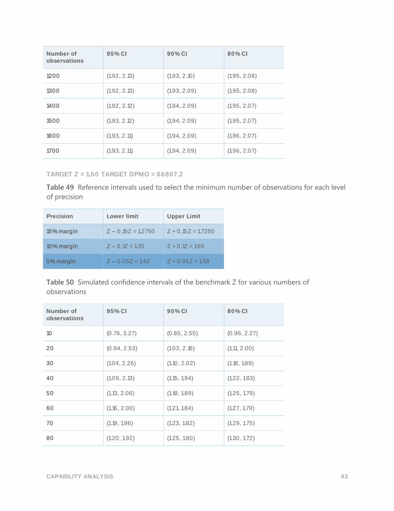
TARGET Z = 1.50 TARGET DPMO = 66807.2
Table 49 Reference intervals used to select the minimum number of observations for each level
of precision
Precision Lower limit Upper Limit
15% margin Z 0.15Z = 1.2750 Z + 0.15Z = 1.7250
10% margin Z 0.1Z = 1.35 Z + 0.1Z = 1.65
5% margin Z 0.05Z = 1.43 Z + 0.05Z = 1.58
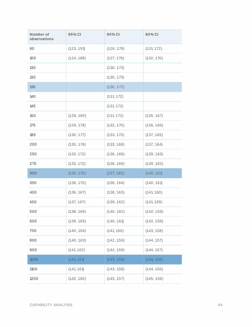
Table 50 Simulated confidence intervals of the benchmark Z for various numbers of
observations
Number of observations
95% CI 90% CI 80% CI
10 (0.76, 3.27) (0.85, 2.55) (0.96, 2.27)
20 (0.94, 2.53) (1.03, 2.18) (1.11, 2.00)
30 (1.04, 2.26) (1.10, 2.02) (1.18, 1.89)
40 (1.09, 2.13) (1.15, 1.94) (1.22, 1.83)
50 (1.13, 2.06) (1.19, 1.89) (1.25, 1.79)
60 (1.16, 2.00) (1.21, 1.84) (1.27, 1.79)
70 (1.19, 1.96) (1.23, 1.82) (1.29, 1.75)
80 (1.20, 1.92) (1.25, 1.80) (1.30, 1.72)
CAPABILITY ANALYSIS 44
Number of observations
95% CI 90% CI 80% CI
90 (1.23, 1.91) (1.26, 1.79) (1.31, 1.72)
100 (1.24, 1.88) (1.27, 1.76) (1.32, 1.70)
130 (1.30, 1.73)
132 (1.30, 1.73)
135 (1.30, 1.72)
140 (1.31, 1.72)
145 (1.31, 1.72)
150 (1.28, 1.80) (1.31, 1.72) (1.35, 1.67)
175 (1.29, 1.78) (1.32, 1.70) (1.36, 1.66)
185 (1.30, 1.77) (1.33, 1.70) (1.37, 1.65)
200 (1.30, 1.76) (1.33, 1.68) (1.37, 1.64)
250 (1.33, 1.72) (1.36, 1.66) (1.39, 1.63)
275 (1.33, 1.72) (1.36, 1.66) (1.39, 1.62)
300 (1.35, 1.70) (1.37, 1.65) (1.40, 1.61)
350 (1.36, 1.70) (1.38, 1.64) (1.40, 1.61)
400 (1.36, 1.67) (1.38, 1.63) (1.41, 1.60)
450 (1.37, 1.67) (1.39, 1.62) (1.41, 1.59)
500 (1.38, 1.66) (1.40, 1.62) (1.42, 1.59)
600 (1.39, 1.65) (1.40, 1.61) (1.42, 1.58)
700 (1.40, 1.64) (1.41, 1.60) (1.43, 1.58)
800 (1.40, 1.63) (1.42, 1.59) (1.44, 1.57)
900 (1.41, 1.62) (1.42, 1.59) (1.44, 1.57)
1000 (1.41, 1.61) (1.43, 1.58) (1.44, 1.56)
1100 (1.41, 1.61) (1.43, 1.58) (1.44, 1.56)
1200 (1.42, 1.60) (1.43, 1.57) (1.45, 1.56)

CAPABILITY ANALYSIS 45
Number of observations
95% CI 90% CI 80% CI
1300 (1.42, 1.60) (1.43, 1.57) (1.45, 1.56)
1400 (1.43, 1.59) (1.44, 1.57) (1.45, 1.55)
1500 (1.43, 1.59) (1.44, 1.57) (1.45, 1.55)
1600 (1.43, 1.59) (1.44, 1.57) (1.46, 1.55)
1700 (1.43, 1.59) (1.44, 1.56) (1.46, 1.55)
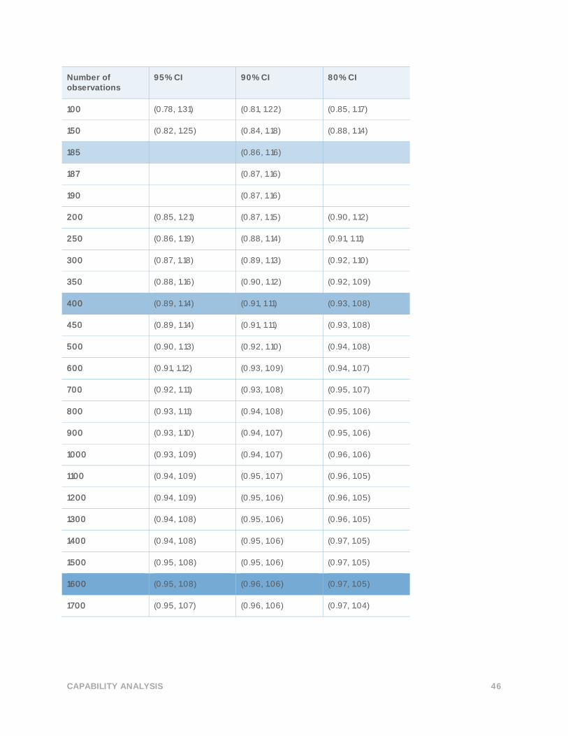
TARGET Z = 1.01 TARGET DPMO = 156247.6
Table 51 Reference intervals used to select the minimum number of observations for each level
of precision
Precision Lower limit Upper Limit
15% margin Z 0.15Z = 0.8585 Z + 0.15Z = 1.1615
10% margin Z 0.1Z =0.91 Z + 0.1Z = 1.11
5% margin Z 0.05Z = 0.96 Z + 0.05Z = 1.06
Table 52 Simulated confidence intervals of the benchmark Z for various numbers of
observations
Number of observations
95% CI 90% CI 80% CI
10 (0.38, 2.33) (0.46, 1.86) (0.55, 1.62)
20 (0.55, 1.83) (0.62, 1.55) (0.68, 1.41)
30 (0.62, 1.63) (0.67, 1.44) (0.74, 1.32)
40 (0.67, 1.54) (0.72, 1.37) (0.77, 1.28)
50 (0.70, 1.45) (0.75, 1.32) (0.80, 1.24)
60 (0.73, 1.42) (0.77, 1.29) (0.82, 1.22)
70 (0.75, 1.38) (0.78, 1.27) (0.83, 1.21)
80 (0.76, 1.35) (0.80, 1.25) (0.84, 1.19)
90 (0.78, 1.32) (0.81, 1.23) (0.85, 1.18)
CAPABILITY ANALYSIS 46
Number of observations
95% CI 90% CI 80% CI
100 (0.78, 1.31) (0.81, 1.22) (0.85, 1.17)
150 (0.82, 1.25) (0.84, 1.18) (0.88, 1.14)
185 (0.86, 1.16)
187 (0.87, 1.16)
190 (0.87, 1.16)
200 (0.85, 1.21) (0.87, 1.15) (0.90, 1.12)
250 (0.86, 1.19) (0.88, 1.14) (0.91, 1.11)
300 (0.87, 1.18) (0.89, 1.13) (0.92, 1.10)
350 (0.88, 1.16) (0.90, 1.12) (0.92, 1.09)
400 (0.89, 1.14) (0.91, 1.11) (0.93, 1.08)
450 (0.89, 1.14) (0.91, 1.11) (0.93, 1.08)
500 (0.90, 1.13) (0.92, 1.10) (0.94, 1.08)
600 (0.91, 1.12) (0.93, 1.09) (0.94, 1.07)
700 (0.92, 1.11) (0.93, 1.08) (0.95, 1.07)
800 (0.93, 1.11) (0.94, 1.08) (0.95, 1.06)
900 (0.93, 1.10) (0.94, 1.07) (0.95, 1.06)
1000 (0.93, 1.09) (0.94, 1.07) (0.96, 1.06)
1100 (0.94, 1.09) (0.95, 1.07) (0.96, 1.05)
1200 (0.94, 1.09) (0.95, 1.06) (0.96, 1.05)
1300 (0.94, 1.08) (0.95, 1.06) (0.96, 1.05)
1400 (0.94, 1.08) (0.95, 1.06) (0.97, 1.05)
1500 (0.95, 1.08) (0.95, 1.06) (0.97, 1.05)
1600 (0.95, 1.08) (0.96, 1.06) (0.97, 1.05)
1700 (0.95, 1.07) (0.96, 1.06) (0.97, 1.04)

CAPABILITY ANALYSIS 47
© 2015, 2017 Minitab Inc. All rights reserved.
Minitab®, Quality. Analysis. Results.® and the Minitab® logo are all registered trademarks of Minitab,
Inc., in the United States and other countries. See minitab.com/legal/trademarks for more information.