Cap and Trade and Structural Transition in the California...

`

4/25/2007 1

DEPARTMENT OFAGRICULTURAL AND RESOURCE ECONOMICS

207 GIANNINI HALL

UNIVERSITY OF CALIFORNIA

BERKELEY, CA 94720

PHONE: (1) 510-643-6362

FAX: (1) 510-642-1099

WEBSITE: are.berkeley.edu

Cap and Trade and

Structural Transition in the

California Economy

David Roland-Holst

April, 2007

Research Paper No. 010701

`

4/25/2007 2

Research Papers on Energy, Resources, and Economic Sustainability

This report is part of a series of research studies into alternative energy and resource

pathways for the global economy. In addition to disseminating original research

findings, these studies are intended to contribute to policy dialogue and public

awareness about environment-economy linkages and sustainable growth. All opinions

expressed here are those of the authors and should not be attributed to their affiliated

institutions.

For this project on Climate Action and the California economy, financial support from

the Energy Foundation is gratefully acknowledged. Thanks are also due for outstanding

research assistance by Christopher Busch, Yihui Chim, Fredrich Kahrl, Michael Mejia,

Shane Melnitzer, Daphne Pallavicini, and Colin Sweeney.

Dallas Burtraw, Alex Farrell, Michael Hanemann, Skip Laitner, Jason Mark, and Marcus

Schneider offered many helpful insights and comments. Opinions expressed here are

the author‘s and should not be attributed to his affiliated institutions.

`

4/25/2007 3

Executive Summary

California has the innovation capacity to achieve its Climate Action objectives without

compromising economic growth, as a variety of official, officially sponsored, and

independent studies have demonstrated. While the state‘s aggregate income and

employment can actually be stimulated by the right package of policies, including a

cap and trade system to reduce CO2 emissions, the structural adjustments that ensue

will be complex and far reaching. While no substantive mitigation policy can be

without some direct and indirect costs, the benefits from greater energy efficiency

and improved environmental conditions can significantly outweigh these. Thus

responsible climate action assessment requires consideration of both the magnitudes

and composition of adjustment costs and benefits. The primary objective of this report

is to strengthen the basis of evidence in this area. To effectively limit costs and

facilitate the innovation needed to sustain and propagate the benefits of a more

carbon-efficient future, policy makers need better visibility regarding adjustment

processes.

This study reviews an extensive body of evidence at the industry level, examining

publically available information on the technology and cost structures of so-called first

and second-tier emitters in California. These sectors are most likely to be included in

a cap and trade system because they make large aggregate or relative contributions to

CO2 emissions and can therefore make important contributions to reducing climate

change risk. Our general finding is that all these sectors can make the needed

contributions, particularly under a well-designed cap and trade system that uses a

market mechanism to more efficiently allocate the burden of adjustment.

More detailed characteristics of the adjustment process remain uncertain, but some

impacts could be substantial at the industry and particularly the plant level. The

actual magnitudes will depend critically on the incentive properties of the policy

design. For example, the degree to which firms pass on adjustment costs to consumers

will depend upon competitive conditions in each industry and the extent to which

policies promote investment in efficiency. If the state is to maintain its leadership as a

dynamic and innovation oriented economy, it is essential that Climate Action policy

`

4/25/2007 4

include explicit incentives for firms to follow competitive innovation discipline,

investing in discovery and adoption of new technologies that offer win-win solutions to

the challenge posed by climate change for their industries and for consumers. In this

way, California can sustain its enormous economic potential and establish global

leadership in the world‘s most promising new technology sector, energy efficiency, as

it has done so successfully in ICT and biotechnology.

`

4/25/2007 5

CONTENTS

1. INTRODUCTION .............................................................................................................................. 7

2. SCENARIOS FOR CLIMATE ACTION ................................................................................................ 11

2.1. ECONOMIC BEHAVIOR AND STRUCTURAL TRANSITION ........................................................................... 11 2.2. PRICE EFFECTS ............................................................................................................................... 14 2.3. SCENARIOS AND RESULTS ................................................................................................................. 20 2.4. SIMULATION RESULTS ..................................................................................................................... 21

2.4.1. Electric Power Sector ............................................................................................................ 26 2.4.2. Cement .................................................................................................................................. 28 2.4.3. Petroleum Refining ............................................................................................................... 30 2.4.4. Chemicals .............................................................................................................................. 31

3. ELECTRICITY .................................................................................................................................. 33

3.1. MODELLING THE BEHAVIOR OF LOAD SERVING ENTITIES ........................................................................ 33 3.2. POWER GENERATION AT THE PLANT LEVEL .......................................................................................... 36

3.2.1. Moss Landing Power Plant ................................................................................................... 41 3.2.2. Delta Energy Center .............................................................................................................. 44 3.2.3. AES Alamitos Generating Station.......................................................................................... 47 3.2.4. Haynes Generating Station ................................................................................................... 50 3.2.5. Coal Plants: Mohave(NV) and Intermountain(UT) ................................................................ 52 3.2.6. Structural Transition in the Electric Power Industry ............................................................. 55

4. CEMENT PRODUCTION IN CALIFORNIA ......................................................................................... 56

4.1. MODELLING APPROACH ................................................................................................................... 56 4.1.1. Data Sources ......................................................................................................................... 58

4.2. OVERVIEW OF INDUSTRIAL STRUCTURE ............................................................................................... 60 4.3. COST DETERMINANTS FOR CEMENT PRODUCERS IN CALIFORNIA ............................................................... 62 4.4. GENERAL EMISSIONS AND ENERGY USE .............................................................................................. 63 4.5. GENERAL EMISSIONS REDUCTION OPPORTUNITIES ................................................................................ 66 4.6. CALIFORNIA SPECIFIC EMISSIONS REDUCTION OPPORTUNITIES ................................................................ 67 4.7. INDIVIDUAL PLANT SURVEY .............................................................................................................. 70 4.8. HOW WILL CEMENT MANUFACTURERS RESPOND TO ADJUSTMENT PRESSURES? ......................................... 73

5. OIL REFINING ................................................................................................................................ 76

5.1. CALIFORNIA REFINERIES: OUTPUT ...................................................................................................... 77 5.2. CALIFORNIA REFINERIES: ENERGY USE AND CO2 EMISSIONS................................................................... 82 5.3. HETEROGENEITY IN CALIFORNIA’S OIL REFINING SECTOR ........................................................................ 85

5.3.1. Tesoro Golden Eagle ............................................................................................................. 87

6. CALIFORNIA CHEMICAL INDUSTRY ................................................................................................ 89

6.1. OVERVIEW .................................................................................................................................... 89 6.2. PRODUCTION STATISTICS ................................................................................................................. 91

ANNEX 1 - OVERVIEW OF THE BEAR MODEL ........................................................................................ 106

STRUCTURE OF THE CGE MODEL ................................................................................................................... 106 PRODUCTION ............................................................................................................................................. 110 CONSUMPTION AND CLOSURE RULE ............................................................................................................... 110 TRADE ...................................................................................................................................................... 111

`

4/25/2007 6

DYNAMIC FEATURES AND CALIBRATION ........................................................................................................... 111 CAPITAL ACCUMULATION.............................................................................................................................. 112 THE PUTTY/SEMI-PUTTY SPECIFICATION ........................................................................................................... 112 DYNAMIC CALIBRATION ................................................................................................................................ 112 MODELLING EMISSIONS ............................................................................................................................... 113

ANNEX 2 – CEMENT INDUSTRY SUPPLEMENTAL DATA ......................................................................... 116

7. REFERENCES ................................................................................................................................ 122

`

4/25/2007 7

Cap and Trade and Structural Transition in the California

Economy

David Roland-Holst1 UC Berkeley

Climate change will have serious impacts on the state of California and is now widely

recognized as an important risk to the economic activities and living standards of

present and future generations. In response to this, the state has extended its long

commitment to sustainable economic growth by implementing a series of initiatives

for energy efficiency and GHG emissions reduction. In the latter category, Assembly

Bill 32 represents landmark legislation to address climate change risks and move the

California economy to a path of greater energy efficiency, productivity, and reduced

environmental risk.

The central provision of AB32 is a set of targets for greenhouse gas (GHG) mitigation,

to be achieved at least in part by a market oriented mechanism like a cap-and-trade

scheme. While cap and trade is widely acknowledged for its potential to enlist market

1 Department of Agricultural and Resource Economics. Correspondence: [email protected].

1. INTRODUCTION

mailto:[email protected]

`

4/25/2007 8

forces and private agency for efficiency improvement, the empirical evidence on

detailed economic impacts of these policies remains weak. In this report, we evaluate

the implications of policies like the proposed CO2 cap and trade system using a

dynamic simulation model of the state economy.

The research reported here extended macroeconomic analysis developed to inform the

legislative dialogue on AB32 during the summer of 2006 (Roland-Holst:2006b). While

the macro results indicated that California‘s growth and environmental objectives can

be reconciled, they did not provide much detail on the structural adjustments that

would attend this process. Perhaps for this reason, some observers (e.g. Stavins et al:

2007) mistakenly interpreted this work as promoting no cost solutions. In fact, any

substantial climate action in California and any other modern economy will entail

costs, but these can be substantially or completely outweighed at the aggregate level

by offsetting benefits. Because detailed costs and benefits may accrue to different

stakeholders, responsible climate action assessment requires consideration of both the

magnitudes and composition of positive and negative adjustment effects. The primary

objective of this report is to strengthen the basis of evidence in this area, and much

more research could be productively undertaken to elucidate effects of complex policy

alternative in greater detail. As part of this effort to better understand the economic

adjustments that might ensue from cap and trade approaches to GHG regulation, a

comprehensive review was conducted of publically available information on

technology and cost structures in the state‘s first and second-tier GHG emitting

industries. These information resources are summarized in four sections of this report,

corresponding to Electric Power, Cement, Petroleum Refining, and Chemicals. While

may insights have been gained in this process, the information in public hands remains

too fragmentary to reliably predict detailed incidence patterns in these sectors.

Despite these limitations, this report attempts to improve general understanding of

the salient forces at work within prominent individual industries. In doing so, it is

possible to reach a variety of important conclusions, if not to identify individual

enterprise winners and losers or plant-specific quantitative adjustments. Such detail

would of course be of interest to enterprises, both those directly affected and those in

competitive or contractual relationships with affected firms, but it is outside the

scope of this analysis.

`

4/25/2007 9

Several important messages for policy makers and stakeholders emerge from this

review and analysis. For example, policies that restrict GHG emissions, while socially

desirable, can lead to unintended adverse effects if they are defined too narrowly.

When they impose new costs on industries, they also risk transferring those costs to

society through the price system. More complete policies will recognize the combined

potential of economic competition and investment in efficient technology to mitigate

new cost/price pressures that arise in targeted industries.

Industries with high levels of competition will experience efficiency gains more

spontaneously, as new entrants and incumbents seeking new market share invest in

competitive innovation voluntarily. In other contexts, investment incentives can be

provided, perhaps from resources generated by pollution licenses. In either case,

explicit recognition and facilitation of the essential role played by innovation can hel

secure win-win outcomes for both industry and society.

At a more detailed level, we draw conclusions about the adjustment process in several

industries. For example, in the face of significant potential cost increases, the electric

power distribution sector is likely to make important compositional adjustments in its

generation portfolio over the next decade. Because the working life of these capital

goods spans several decades, these decisions will establish new baselines for emission

intensity and accelerate the need for future efficiency improvements.

In the cement sector, we infer that conformity to new GHG standards, even under

relatively efficient cap and trade regimes, will confer nontrivial costs on this sector,

and these will either be passed on to consumer, reinforce innovation incentives, or

some combination of the two. Another unresolved issue in this sector concerns the

potential of blended cement to offset this sector‘s carbon liability. The industry‘s

largest individual customer, a public agency, is undecided about whether or not

blended cement will meet its needs. This deadlock poses an important obstacle to the

industry‘s strategy for meeting the state‘s own environmental objectives, and it also

denies the cement market and essential precedent of adoption. Finally, there has

been considerable discussion about the long term viability of within-state cement

operations. It should be noted, however, that in no scenario we consider do Climate

Action costs approach the kind of pressures the sector has repeatedly experienced

`

4/25/2007 10

from its energy fuel inputs. For this reason, it is difficult to imagine California‘s

cement industry experiencing any relocation adjustments.

Oil refining is an exceptionally challenging industry for analysis because of the

diversity of its product mix and pervasive linkages across the economy. Because it is

the primary channel for GHG production by all forms of transportation and a

significant component of other manufacturing activities, its response to GHG policies

will have a very significant indirect component. Indeed, indirect mitigation of refinery

emissions from attenuation of fuel demand trends can account for up to half this

sector‘s GHG mitigation. This being said there are still significant opportunities for

process innovation to achieve higher efficiency levels in this sector, although

restrictions on new capacity development may retard this process.

The chemicals sector is another example of a very diverse sector with strong indirect

linkages. As a California manufacturing sector, it is second in GHG emissions only to

Petroleum refining. Despite this, the largest component of the industry,

pharmaceuticals, bears indirect responsibility for most of its GHG emission through

electricity and energy intensive input demands. Opportunities for process innovation

are considerable across this sector, but it is clear that no single prescription for

technological change or other structural transition will fit all cases in such a diverse

environment. More than any industry considered in this study, chemicals demonstrates

the value of market oriented policies that enlist private agency to find individual

solutions that fulfill public objectives.

In the next section, we discuss the scenarios used to study cap and trade‘s economic

effects in California, with particular reference to the so-called First-tier Emitter

sectors. Following this, we discuss each major sector in greater detail, reviewing

available data on industry structure and conduct and explaining how each sector was

implemented in the model. Section 3 covers the Electricity Production and Distribution

sector, followed in Sections 4-6 by Cement, Oil Refining, and Chemicals. The report

closes with summary remarks and a discussion of how this framework will be extended

to provide more extensive support for climate action policies.

A series of annexes follows the main study. The first of these provides a general

description of the Berkeley Energy and Resources (BEAR) model, which is fully

`

4/25/2007 11

documented in (Roland-Holst:2005). Also included, in the order of industry

presentation in the study, are subsidiary tables and data sources.

California has well-established leadership in policies related to climate change,

including a broad spectrum of energy and emissions initiatives that have set national

standards for economic growth through innovation and efficiency. These policies have

targeted energy efficiency and air pollution from many different angles, including

vehicle, appliance, and building standards, tax credits, and now economywide

emissions targets. While the approaches are diverse, most of these policies share the

important objective of seeking to influence economic behavior in ways that limit

adverse environmental consequences. Thus climate action policies seek to change

behavior, which in turn alters economic structure by inducing agents to choose

different technologies, goods and services, and other modalities of economic behavior.

2.1. Economic Behavior and Structural Transition

To understand these induced adjustments, we focus on a triad of behavioral elements

(Figure 2.1): Household consumption/adoption, Firm investment/adoption, Firm price

setting. Consider a cap and trade policy that imposes a ceiling on GHG emissions,

allowing firms to buy permits if they exceed their initial allowances. If the ceiling is

binding, the policy gives rise to a new cost in the economy, having created a market

for a negative externality. What this represents is the cost of re-allocating pollution

rights that were until now unpriced. In response to the new cost, firms have two

options, to increase prices or efficiency levels. In the first case, the firm must have

sufficient market power to pass through the cost to prices paid by downstream buyers

of their product. The second option requires firms to invest in technology adoption

that will reduce emissions, increase profits, or both, to offset the new cost. In

general, it is reasonable to expect an industry to adapt with a combination of price

2. SCENARIOS FOR CLIMATE ACTION

`

4/25/2007 12

and investment/adoption responses, but this depends on market conditions and

technology choices.

The third corner of the triad, consumers, would respond in the event of a price

increase for the good or service in question, or if product standards were mandated to

them. In these cases, they too face an investment/adoption decision, the prospect of

incurring a fixed up-front cost to reduce long term dependence on a more expensive

commodity. Their willingness and ability to do this will depend on the (long term)

credibility of the price adjustment or policy, their purchasing power, and technology

choices available to them.

Figure 2.1: The Policy Response Triad

Within the universe of policy responses, the three areas A, B, and C represent

fundamentally different adjustment mechanisms. In region B, firms absorb most of the

adjustment with a combination of price increases and investments in more efficient

technology. Households are relatively insensitive to the price changes, and their

demand patterns change relatively little, as was the case, for example, with recent oil

price increases and rising home construction costs over the recent low interest rate

cycle. In circumstances like this, demand driven sectors like electricity, refined

Firm Price

Increase

A

B

C

Consumer Demand/ Adoption

Firm Investment/

Adoption

`

4/25/2007 13

petroleum, and cement are more likely to maintain stable output trends and long term

profitability, largely through passing on increased cost (left side of region B),

efficiency improvements (right side) and combinations of these. Because, for the first-

tier emitting industries, GHG efficiency is largely about energy efficiency, the long

term savings for firms from technology adoption could be substantial if energy prices

trend higher. In this context, cap and trade policies promise a double dividend.

Sections A and C imply more significant demand side adjustment, with more uncertain

effects on statewide output, employment, and incomes. To the extent that households

adopt efficiency improving technologies (cars, appliances, etc.), they can offset rising

prices (A) or actually save money (C) to stimulate other forms of consumption. In the

CAT scenario analysis (Roland-Holst:2006A), for example, induced household efficiency

gains from mandatory standards (e.g. Pavley) produced significant personal energy

savings. These were then reallocated to other consumption and, because this was

more likely to be on in-state goods and services, GSP and state employment were

stimulated.

Figure 2.2: Structural Transition

Firm Price

Increase

Firm Investment/

Adoption

A

B

C

Consumer Demand/ Adoption

`

4/25/2007 14

Ultimately, all three components of structural adjustment will come into play.

Generally speaking, the short run responses will be instigated by firms, since they are

the original targets of the policy. Their first response, to the extent markets permit,

will be to raise prices. As time passes, they will migrate (Figure 2.2, yellow arrow)

toward new technology that enables their industry to return to competitiveness. This

process, enshrined in the economic theories of competition, will arise from a

combination of firm entry and adoption by incumbents to compete against or even

deter such entrants. The speed by which competitive conditions are restored depends

critically on the initial competitive conditions. If markets are too concentrated or

entry barriers too high, this component of structural transition could proceed very

slowly.

Meanwhile, consumers will respond to the initial price increase in two stages. In the

short term, they can be expected to engage in demand smoothing, absorbing higher

prices temporarily to prevent sudden changes in lifestyle. If price changes persist,

however, this will be followed by decisions to change consumption patterns, including

adoption of technologies that reduce dependence on higher priced goods (Figure 2.2,

green arrow). The combination of these two trends yields the basic structural

transition arising from cap and trade, the introduction of new private costs that more

fully account for public costs of climate change risk.

2.2. Price Effects

To what extent can firms pass on the cost of regulation? This depends almost

completely on the degree of their market power, sometimes called monopoly power.

Clearly firms have a strong incentive to do this, since it would be a most economical

way of neutralizing regulatory cost with no changes in operations or management

practices. Of course their ultimate profit and output conditions are unlikely to remain

neutral, since consumers will react in some way to a price pass through.

In any case, history can give us some guidance about pass through from production

costs to prices even if the information is only inferential. In the cement industry, as in

most emission-intensive industries, energy costs are a prominent or even dominant

`

4/25/2007 15

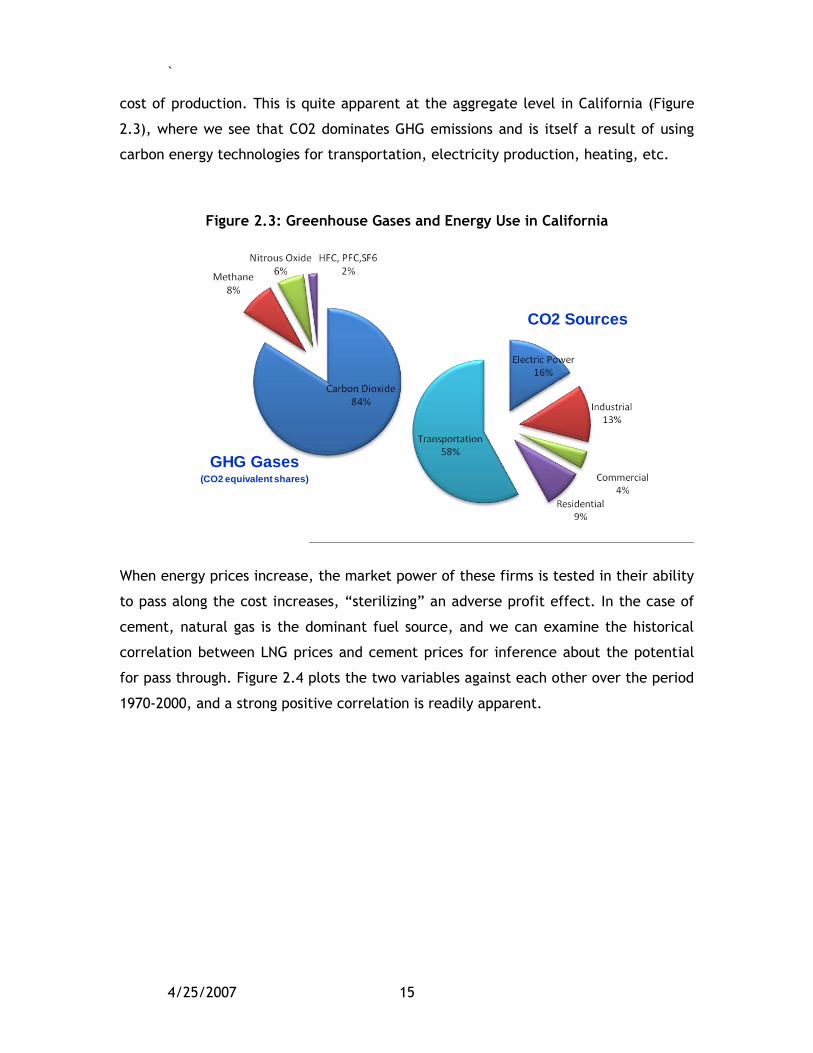
cost of production. This is quite apparent at the aggregate level in California (Figure

2.3), where we see that CO2 dominates GHG emissions and is itself a result of using

carbon energy technologies for transportation, electricity production, heating, etc.

Figure 2.3: Greenhouse Gases and Energy Use in California

GHG Gases(CO2 equivalent shares)

CO2 Sources

When energy prices increase, the market power of these firms is tested in their ability

to pass along the cost increases, ―sterilizing‖ an adverse profit effect. In the case of

cement, natural gas is the dominant fuel source, and we can examine the historical

correlation between LNG prices and cement prices for inference about the potential

for pass through. Figure 2.4 plots the two variables against each other over the period

1970-2000, and a strong positive correlation is readily apparent.

`

4/25/2007 16

Figure 2.4: National Cement and LNG Prices, 1970-2000

0

10

20

30

40

50

60

70

80

90

0 1 2 3 4 5 6 7

Ce

me

nt

Pri

ce($

/T)

LNG Price

To characterize this relationship more precisely, we regressed Cement prices against

LNG prices, both in logarithmic form, and the results are presented in Table 2.1

summarizes the results. The relevant estimate is labeled the Coefficient of the X

variable, which in this case denotes the historical elasticity of Cement prices with

respect to LNG prices. This estimate indicates that, in percentage terms, Cement

prices have risen at about half the rate of LNG prices over time. This percentage is

larger than LNG‘s cost share in Cement production, and significantly so. Thus it

appears that, were other conditions to remain constant over the period considered,

Cement producers would be able to offset most or all energy price increases by

passing them on to consumers. We know, however, that other cost components in

Cement have risen steadily over time, so this elasticity is an over-estimate of LNG

price effects on the sector under consideration. We still concluded, however, that a

significant degree of market power and pass through is possible in this sector.

`

4/25/2007 17

Table 2.1: Cost Price Elasticities for LNG and Cement, 1970-2000

Regression Statistics

Multiple R 0.96

R Square 0.91

Adjusted R Square0.91

Standard Error 0.05

Observations 31

ANOVA

df SS MS F

Regression 1 0.77 0.77 308.45

Residual 29 0.07 0.00

Total 30 0.84

CoefficientsStandard Error t Stat P-value

Intercept 1.42 0.02 79.13 0.00

X Variable 1 0.53 0.03 17.56 0.00

Elasticity estimation supports an empirical argument for cost pass through, but

economic theory describes it as the result of combined supply and demand conditions.

To compare this perspective, consider the examples in Figure 2.5 below, which depict

supply and demand curves in the presence of a fixed increase to industry marginal cost

(MC->MC‘). When the supply curve on the right shifts upward, consumers and firms

share the burden of increased cost (areas C and F). On the other hand, when supply is

demand driven and highly elastic, as on the left, consumers bear all the increased

cost.

Using the case of the Cement industry again, Figure 2.6 plots national output against

inflation adjusted prices over the thirty year period 1970-2000. These figures suggest

very strongly that Cement is a demand driven industry, and that the incidence of cost

shocks can be passed on to consumers.

Thus we see from two perspectives that cost pass through to prices can occur, at least

in the short run. In the face of process related cost shocks such as GHG regulation

then, it is reasonable to expect firms to increase prices until they can make the

efficiency improvements needed to return to competitiveness. Consumers will then

react according to their short run demand elasticity. This could mean they are

`

4/25/2007 18

unresponsive in the short run, either because the price increase is not credible in the

long term or they want to smooth consumption while planning technology adoption. In

the longer term, if prices remain high they will contribute to structural transition by

shifting consumption away through increased efficiency or substitution. Meanwhile,

competitive firms will be shifting industry technology through their own structural

transition, including firm entry, exit, and incumbent investments in more efficient

technology. As the fixed costs of these investments and disinvestments are made,

industry average costs will come back down toward a longer term equilibrium value,

and some demand will be restored.

In a world of innovation and efficient capital markets, this structural transition can

happen in a matter of a few years. If cap and trade policies are phased to take

account of this, the adjustment process can be relatively smooth. For all this to work,

both stakeholders and policy makers need reliable information about all these

adjustment components. In this section, we use scenario analysis with the BEAR model

to give indications about the magnitude and incidence patterns of structural

transition, as it would arise from a cap and trade GHG mitigation regime.

`

4/25/2007 19

Figure 2.5: Cost Pass Through under Alternative Supply Conditions

Figure 2.6: Cement Industry Supply, 1970-2000

0

20

40

60

80

100

120

140

60 65 70 75 80 85 90

Un

it p

rice

(9

8$

/T)

Production (MT)

S=MC P’

p F

C

Q

C

P’

Partial Pass Through Complete Pass Through

S’=MC’

p

D D

S’=MC’

S=MC

Q

`

4/25/2007 20

2.3. Scenarios and Results

In this section, we present a series of policy scenarios for climate action and discuss

their implications for economic growth and structural transition of the California

economy. In particular, we use the BEAR model for a more detailed assessment of

California‘s cap and trade initiative, examining the interplay of each of the three

components of structural transition discussed above (Figure 2.1). Unlike engineering

and partial equilibrium analyses of environmental policies, this approach elucidates

the interactions of firms and consumers across a spectrum of the state‘s economic

activities and markets, where agents have a wider scope of choice and their extensive

indirect linkages to other economic activities can be taken into account. The model

also operates at a high level of detail to avoid aggregation bias that can mask spillover

effects between sectors, stakeholders, and winners and losers.

The scenarios discussed here have already been studied in terms of aggregate

economic effects in Roland-Holst (2006), but the present analysis goes deeper into the

industry, factor market, and household effects of climate action policies like the cap-

and-trade scheme considered here, using the BEAR model‘s detailed specification to

better understand the complex patterns of structural incidence arising from these

policies. As in the aggregate study, seven scenarios, summarized in Table 2.2, are

evaluated.

The CAT scenario reflects a package of climate action initiatives recommended to the

Governor by CalEPA in January, 2006. To these are added a cap-and-trade scheme

with progressive sector inclusion (Table 2.4). In scenarios 2-5, permits are auctioned

and firms adjust to the cap from their own resources. This approach increases the

likelihood of adapting by passing on higher costs to consumers. In the last two

scenarios, firms are allowed rebates of their permit costs if these are reinvested in

efficiency enhancing new technology. The result is endogenous technical change that

alters the structure of production toward higher efficiency, offsetting the adjustment

costs for producers, consumers, and the economy as a whole.

`

4/25/2007 21

Table 2.2: Policy Scenarios for Climate Action

2.4. Simulation Results

Aggregate impacts of the above scenarios have already been discussed in Roland-Holst

(2006b), and are reproduced here only for convenience. Table 2.3 summarizes the

variables of primary interest, GHG emissions, statewide real GSP and employment

growth. Results are displayed as percentage changes with respect to the Baseline

(scenario 1) in the final year (2020).

1. Baseline (no emission reduction target) [1]

2. 8 CAT policies (direct regulation) [2}

3. CAT policies plus emission cap to meet remainder of 2020 target

a. Industries in Group 1 covered by an aggregate cap [3]

b. Industries in Groups 1 and 2 covered by an aggregate cap [4]

c. Industries in Groups 1, 2 and 3 covered by an aggregate cap [5]

4. 8 CAT policies plus emission cap on industries in Groups 1, 2 and 3 with revenues recycled into

innovation investment [6]

5. 8 CAT policies plus emission cap on all emitting industries with revenues recycled into innovation

investment [7]

`

4/25/2007 22

Table 2.3: Macroeconomic Impacts

Scenario 2 3 4 5 6 7

CAT Group1 Group12 Group123 G123Gr AllIn

Total GHG* -13 -28 -28 -28 -28 -28

Household GHG* -32 -32 -32 -32 -31 -30

Industry GHG* -3 -26 -26 -26 -26 -27

Annual GSP Growth* 2.4 2.4 2.4 2.4 3.1 4.7Employment* .10 .06 .08 .08 .44 1.07

*Percent change from Baseline scenario in the year 2020.

Jobs (thousands) 20 13 16 17 89 219

Percent of GHG Target 47 101 100 100 100 100

The CAT scenario (2) was discussed in detail in Roland-Holst (2006a) and it suffices

here to note only its general characteristics. Implementing just eight leading CAT

policies has the potential to achieve about half of the California‘s targeted 2020

emissions reductions, while at the same time stimulating state output and

employment. The economic stimulus results from the dynamic gains that arise when

demand is diverted to more California-intensive expenditure as energy efficiency saves

money for households and industry, promoting state economic growth. This result can

be contrasted with a static Ricardian model, where international resource constraints

impose offsetting terms-of-trade adjustments on import substitution. In an open ended

dynamic scenario, retained state expenditures have multiplier effects that compound

domestic income, saving, and employment growth. 2

Expanding beyond the CAT scenario, we examine a progressively larger coverage of a

cap on emissions designed to make up the remaining reduction in emissions . The

three industries in Group 1 are frequently identified as the core sectors for a GHG cap.

Our results for Scenario 3 suggest, however, that these sectors almost certainly

should not bear the burden of adjustment to the 2020 targets alone. Indeed, BEAR

estimates of their baseline GHG emissions for 2020 are about 173MMT, while hitting

2 The dynamic benefits of energy import substitution have been corroborated by the Climate Action Team in its in-house economic analysis of these policies. Compare also RFF et al (2007). Other authors have challenged these findings (e.g. Stavins et al:2007), but their concerns relate mainly to data quality and meager evidence for alternative outcomes has been provided to date.

`

4/25/2007 23

the target would require about 90MMT in emission reductions, an implied annual

reduction in sectoral intensity of over 3.5% (see Table 4.3). For this reason, the

scenario appears infeasible on a sustained intensity reduction basis, resulting in

slightly lower annual real GSP growth and employment statewide.

When the scope of industry coverage is expanded to include the nine industries in

Group 2, Scenario 4, the results are much more encouraging. In this scenario, the nine

sector group could meet the governor‘s 2020 targets with less than 3% annual

improvements in average emission intensity.3 While this seems a feasible aggregate

objective, however, it is important to recognize that the adjustment burden will fall

differently on different sectors, depending on their initial intensity and share of the

mitigation they must achieve. One of the advantages of detailed simulation models

like BEAR is that they capture these important compositional effects, and in Table 4.3

we see how increasing scope diffuses the burden of adjustment.

In this scenario, the nine sectors responsible for meeting the target will have to

reduce emission intensity by up to 3.65% per annum, sustaining this over a nine year

period. This level, too, will be difficult to sustain. Even when scope is extended to all

industries, Scenario 5, nine year average annual efficiency gains of over 2.9% would be

needed.

The main alternative to this would be extending regulation to services and mobile

sources or to orchestrate the present scenario with other GHG policies, yet the all-

inclusive Scenario 7 indicates this would still require more than 2% annual mitigation

and the administrative feasibility of such a program is very doubtful.

The results in Scenarios 5-7 results are broadly consistent with what is assumed in

some other policy analyses. For example, the President‘s climate change policy for

voluntary GHG emission intensity reductions stipulates 2% mitigation per year for ten

years (Abraham, 2004), and this goal is approximately in line with historical national

trends. California itself has experienced approximately a 2% decline in GHG intensity

from 1990-2000 (Climate Action Team, 2006). It must be recalled, however, that these

3 Note in Table 4.3 that several sectors have much higher annual intensity reductions, some over 4.5%, because of legacy effects from being targeted by CAT policies.

`

4/25/2007 24

scenarios include some mandatory (direct regulation) CAT policies. The clear message

is that California must take policy initiative to achieve these overall levels of

abatement.

From Scenarios 2 - 5, we can draw a few salient inferences. Firstly, industry-oriented

GHG mitigation needs to be relatively inclusive if the adjustment burden is to be

manageable. Second, this category of policy needs to be coordinated with other

substantial commitments to GHG efficiency (e.g. CAT regulatory policies). In the case

considered here, where an inclusive industry policy is combined with other GHG

regulatory initiatives, we find that industry must still improve energy efficiency and

GHG gas intensity substantially. Although the implied rates of improvement are

probably feasible, they appear to be significantly outside the range of voluntary

compliance. The apparent need for more determined and directed mitigation schemes

brings us to Scenarios 6 and 7.

`

4/25/2007 25

Table 2.4: Alternative Industry Emission Groups

1. Group 1: First-tier Emitters A04DistElc Electricity Suppliers A17OilRef Oil and Gas Refineries A20Cement Cement

2. Group 2: Second-tier Emitters A01Agric Agriculture A12Constr Construction of Transport Infrastructure A15WoodPlp Wood, Pulp, and Paper A18Chemicl Chemicals A21Metal Metal Manufacture and Fabrication A22Aluminm Aluminium Production

3. Group3: Other Industry Emitters A02Cattle Cattle Production A03Dairy Dairy Production A04Forest Forestry, Fishery, Mining, Quarrying A05OilGas Oil and Gas Extraction A06OthPrim Other Primary Activities A07DistElec Generation and Distribution of Electricity A08DistGas Natural Gas Distribution A09DistOth Water, Sewage, Steam A10ConRes Residential Construction A11ConNRes Non-Residential Construction A13FoodPrc Food Processing A14TxtAprl Textiles and Apparel A16PapPrnt Printing and Publishing A19Pharma Pharmaceuticals A23Machnry General Machinery A24AirCon Air Conditioner, Refrigerator, Manufacturing A25SemiCon Semiconductors A26ElecApp Electrical Appliances A27Autos Automobiles and Light Trucks A28OthVeh Other Vehicle Manufacturing A29AeroMfg Aeroplane and Aerospace Manufacturing A30OthInd Other Industry

`

4/25/2007 26

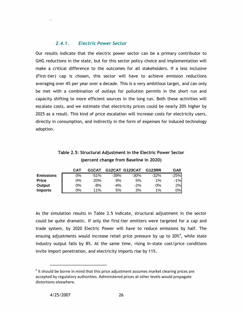
2.4.1. Electric Power Sector

Our results indicate that the electric power sector can be a primary contributor to

GHG reductions in the state, but for this sector policy choice and implementation will

make a critical difference to the outcomes for all stakeholders. If a less inclusive

(First-tier) cap is chosen, this sector will have to achieve emission reductions

averaging over 4% per year over a decade. This is a very ambitious target, and can only

be met with a combination of outlays for pollution permits in the short run and

capacity shifting to more efficient sources in the long run. Both these activities will

escalate costs, and we estimate that electricity prices could be nearly 20% higher by

2025 as a result. This kind of price escalation will increase costs for electricity users,

directly in consumption, and indirectly in the form of expenses for induced technology

adoption.

Table 2.5: Structural Adjustment in the Electric Power Sector

(percent change from Baseline in 2020)

CAT G1CAT G12CAT G123CAT G123RR GAll

Emissions 0% -51% -39% -30% -32% -25%

Price 0% 20% 9% 5% 1% -1%

Output 0% -8% -4% -2% 0% 2%

Imports 0% 11% 5% 3% 1% 0%

As the simulation results in Table 2.5 indicate, structural adjustment in the sector

could be quite dramatic. If only the first-tier emitters were targeted for a cap and

trade system, by 2020 Electric Power will have to reduce emissions by half. The

ensuing adjustments would increase retail price pressure by up to 20%4, while state

industry output falls by 8%. At the same time, rising in-state cost/price conditions

invite import penetration, and electricity imports rise by 11%.

4 It should be borne in mind that this price adjustment assumes market clearing prices are accepted by regulatory authorities. Administered prices at other levels would propagate distortions elsewhere.

`

4/25/2007 27

More inclusive caps will defray this adjustment burden to other sectors, prices, and

commodity classes, but without investment incentives the overall ―new‖ cost of the

cap and trade scheme will impose efficiency costs on the state economy. The key to

averting this is promotion of innovation and technology adoption, as can be clearly

seen in the last two scenarios. When cap and trade policies provide rebates for

investment and adoption of more efficient technology, the result is neutralization

cost/price inflation and sustained growth.

Having said this, it is important to note that structural change will have more detailed

costs, even when industrywide and statewide nets benefits are realized. To see this,

note the dispersion of efficiency levels in the states, existing generation capacity, as

depicted in Figure 2.7 for the largest generation sites, together representing half of

California‘s capacity. Even within the natural gas generation cohort, observed

efficiency levels can vary by a factor of two. Clearly, the Load Serving Entities (LSEs)

will have strong incentives to shift their portfolios across these sources (from right to

left) as they come under increasing GHG regulation. This kind of shifting will drive up

capacity use and costs from the more efficient sources, but in any case is likely to be a

first alternative to new investments in the short and medium term. The exact

composition of this shift would be very useful to anticipate, both for the sake of

private stakeholders and public agencies who might be able to mitigate the ensuing

adjustment costs. It cannot, unfortunately, be estimated from publicly available

information.

`

4/25/2007 28

Figure 2.7: Emission Rates and Production Efficiency

Delta

La Paloma

Moss LandingHaynes

Morro Bay

Scattergood

Etiwanda & AES RedondoAES Alamitos

Mohave

Intermountain

0

0.1

0.2

0.3

0.4

0.5

0.6

0 0.2 0.4 0.6 0.8 1 1.2

Pro

du

cti

on

Eff

icie

ncy

Ra

te

Emission to Output Ratio (tCO2/MWh)

2.4.2. Cement

The Climate Action mitigation policies in the cement sector can make modest but

important contributions to reducing statewide emissions. If all the above measures are

adopted, about 2.5% of total emissions can be eliminated on an annual basis. At the

same time, the direct and indirect macroeconomic and industry level effects of the

first four polices are small but negative. In the cap and trade scenarios, we see a

classic example of the challenge posed by structural transition. If incumbent firms in

the industry merely pass on their increased cost, sectoral output and employment will

be adversely affected. If cap and trade phase-ins include incentives for investment

and technology adoption, both the sector and the state economy will again benefit.

Table 2.6 outlines final year real adjustments for the Cement industry, and these

results significantly resemble Electric Power. As with the latter industry, significant

GHG mitigation translates into notable cost/price pressure, but here less than one

third the percentage increase, and only a 2% induced decline in the trend for industry

`

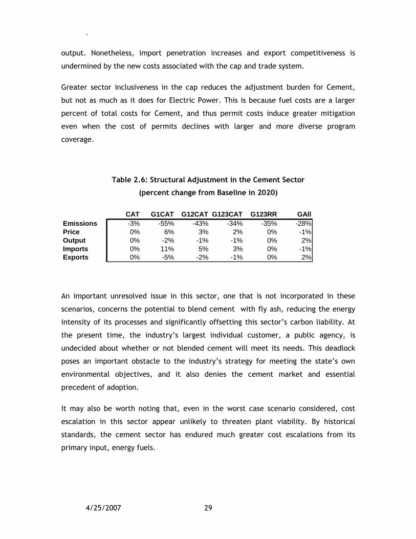
4/25/2007 29

output. Nonetheless, import penetration increases and export competitiveness is

undermined by the new costs associated with the cap and trade system.

Greater sector inclusiveness in the cap reduces the adjustment burden for Cement,

but not as much as it does for Electric Power. This is because fuel costs are a larger

percent of total costs for Cement, and thus permit costs induce greater mitigation

even when the cost of permits declines with larger and more diverse program

coverage.

Table 2.6: Structural Adjustment in the Cement Sector



Emissions -3% -55% -43% -34% -35% -28%

Price 0% 6% 3% 2% 0% -1%

Output 0% -2% -1% -1% 0% 2%

Imports 0% 11% 5% 3% 0% -1%

Exports 0% -5% -2% -1% 0% 2%

An important unresolved issue in this sector, one that is not incorporated in these

scenarios, concerns the potential to blend cement with fly ash, reducing the energy

intensity of its processes and significantly offsetting this sector‘s carbon liability. At

the present time, the industry‘s largest individual customer, a public agency, is

undecided about whether or not blended cement will meet its needs. This deadlock

poses an important obstacle to the industry‘s strategy for meeting the state‘s own

environmental objectives, and it also denies the cement market and essential

precedent of adoption.

It may also be worth noting that, even in the worst case scenario considered, cost

escalation in this sector appear unlikely to threaten plant viability. By historical

standards, the cement sector has endured much greater cost escalations from its

primary input, energy fuels.

`

4/25/2007 30

2.4.3. Petroleum Refining

Oil refining is a major part of the California economy, both in terms of output and

employment, but also in terms of demand for its final products. The refining sector

accounted for 5% of California manufacturing sales in 1997, and the sector employs

nearly 10,000 people.5 On the demand side, California is the largest consumer of

gasoline in the U.S. (11.3% in 2004), and second largest consumer of the country‘s jet

fuel (17.7%); 40% of California‘s 2003 energy consumption was used for

transportation.6

Table 2.7: Structural Adjustment in the Petroleum Refining Sector



Emissions 0% -46% -36% -28% -30% -23%

Price 0% 6% 3% 2% 1% -2%

Output 0% -2% -1% -1% 0% 2%

Imports 0% 3% 1% 1% 1% 0%

Exports 0% -5% -2% -1% -1% 2%

Cap and trade effects in this sector are complex because of the diversity of its product

stream, relatively low demand elasticities, and its pervasive linkages across the

economy. In addition to its direct effluent potential, this sector is the primary channel

for carbon fuels to reach the transport sector, so there are important feedback effects

to refining from any measures that increase fuel efficiency elsewhere in the economy.

Despite its complexity, the industry results for petroleum refining aggregate to

resemble those of a typical energy-intensive manufacturing sector. On an average

basis, however, the experience of this sector is intermediate between that of the two

already considered. Again we see the potential challenge and opportunity posed by

structural transition. If incumbent firms must bear their entire share of the cost of a

cap and trade scheme, their prices can be expected to rise 6% by 2025, with

5 Ernst Worrell and Christina Galitsky, 2004, “Profile of the Petroleum Refining Industry in California,” LBNL-55450. 6 Energy Information Administration (EIA) State Energy Profiles, online at: http://tonto.eia.doe.gov/state/state_energy_profiles.cfm?sid=CA#Con.

`

4/25/2007 31

predictable effects on demand and supply. If instead they are part of an investment

oriented policy package, price effects will be negligible.

Meanwhile, the diversity of technology in this sector means that structural transition

may create winners and losers among incumbent firms. This will depend upon the

market power of individual refiners, as well as their ability to take advantage of

investment incentives.7

2.4.4. Chemicals

The chemical sector will be discussed briefly here as an instructive example of a

second-tier emissions source. While the experience some contraction under the first-

tier scenario because of energy price escalation (Table 2.8), they are negligibly

affected by adapting to inclusion in a cap and trade scheme. The reasons for this are

many. A high level of competitiveness in this sector limits price pass through, high

autonomous investment and technology adoption rates, and extensive scope for own

efficiency improvements all support a relatively smooth adjustment process. Indeed,

this sector‘s own innovation capacity makes it poised to benefit from the incentive

oriented policies in the last two scenarios, stimulating both in-state output and export

competitiveness for California chemicals.

Table 2.8: Structural Adjustment in the Chemical Sector



Emissions 0% -1% -42% -33% -33% -26%

Price 0% 0% 0% 0% -1% -2%

Output 0% -1% -1% 0% 2% 3%

Imports 0% 0% 0% 0% 0% 1%

Exports 0% 0% 0% 0% 1% 3%

7 It should be emphasized that this sector is under very strict regulation regarding new capacity creation, and thus its ability to adopt new technology, even if the objective is greater energy/GHG efficiency, is open to question.

`

4/25/2007 32

As explained in more detail below, chemicals play an important role in statewide

emissions, but they do so as much because of their demand for energy intensive

products (e.g. electricity) as because of direct GHG effluent from the sector itself.

Chemicals are the second largest energy consumer among the state‘s manufacturers,

and for this reason mitigation potential from energy efficiency is considerable. While

the industry as a whole appears to have structural flexibility, it is reasonable to expect

winners and losers to emerge as competitive forces bring forward new technologies

and the resultant cost savings confer strategic advantage on early adopters.

Unfortunately, publically available information on plant-specific cost/technology

structures is quite limited, making it impossible to estimate within-sector tradeoffs.

`

4/25/2007 33

Accounting for 16% of California registered CO2 emissions, the electric power sector

will play an essential role in meeting the state‘s GHG targets. To better understand

this essential strategic sector, we consider it in two parts. First, we discuss

distributors of electricity, an industry dominated by three Load Serving Entities (LSE‘s)

and a large and diverse group of smaller electricity distributors. Demand by the LSE‘s

ultimately determines patterns of emissions from electric power generation, so they

are likely targets of any policies to mitigate emissions from power generation, and

their behavior and contracting activities need to be understood. After an overview of

the distributors, we move back up the electricity supply chain to the generating

technologies themselves. Here plant characteristics will be the primary determinants

of structural adjustment, with more efficient plants in a better position to adapt to

regulatory change in a cost effective manner.

3.1. Modelling the Behavior of Load Serving Entities

A standard economic simulation framework models industrial and service activities

with one representative firm per sector, assuming production arises from neoclassical

assumptions of profit maximization and perfect competition. For a variety of reasons,

this paradigm is not an accurate or even reliably approximate reflection of the

structure and conduct of the electricity distribution sector. When elaborating a

standard economic model for this purpose, three salient characteristics need to be

taken into account:

1. Larger LSE‘s are not firms are representable by a single homogeneous

production function, but distinct entities with delineated markets who draw

their supply from a portfolio of generation technologies.

2. Output prices in this sector are rigid.

3. ELECTRICITY

`

4/25/2007 34

3. Because of the economic costs of supply uncertainty, this sector maintains

substantial excess capacity.

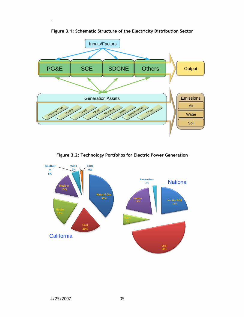
Schematically, the market structure of this sector is described in Figure 3.1 below.

There are three leading LSEs, Pacific Gas and Electric, Southern California Edison, and

San Diego Gas and Electric. The fourth LSE represents an aggregate of all other

electricity distributors. Each of these hires its own factors of production (labor capital)

and draws upon portfolio of in-state and out-of-state generation technologies,

extracting electricity supply from them by direct ownership or contracts for delivery.

In response to the special characteristics listed above, the BEAR model adds special

structural features for this sector. These include the following characteristics:

Individual firm specification for each of the four LSE‘s in Figure 3.1.

1. Fixed prices in a demand-driven market.

2. In the short run, LSE‘s choose the level of capacity utilization.

3. In the long run, LSE‘s choose capacity via investment and contracting.

The California electricity generation system is one of the largest contributors to

greenhouse gas emissions in the state. In looking at the top tier producers (totaling

41% of California generation capacity8), it is apparent that California suppliers may be

better able to adapt to forthcoming carbon restrictions. In today‘s California

electricity industry, portfolio decisions by the LSE‘s have led to capacity that is

significantly less carbon-intensive than national averages. As Figure 3.2 indicates,

California electric power relies significantly less on coal, more on hydro and natural

gas than does the nation as a whole (including California). Renewable technologies

have also emerged more strongly in the state.

8 http://www.energy.ca.gov/

`

4/25/2007 35

Figure 3.1: Schematic Structure of the Electricity Distribution Sector

Generation Assets

SDGNEPG&E SCE Others

Inputs/Factors

Output

Emissions

Air

Water

Soil

Figure 3.2: Technology Portfolios for Electric Power Generation

California

National

`

4/25/2007 36

3.2. Power Generation at the Plant Level

This is not to say, however, that the electricity sector will not face significant

obstacles. Many of California‘s critical electrical plants rely on older technologies that

do not maximize fuel efficiency. Inefficient fuel utilization presents the source of

greatest risk for survival of a plant in a cap-and-trade regulatory environment. This is

because the average fuel cost of production ($/MWh) dominates marginal cost of

production for each and every one of these plants. Their ability to produce and sell

their output competitively, either to LSE‘s though contracts or for them if they are

wholly-owned capital assets, depends critically on this. In a market facing rising fuel

cost trends, inefficient fuel utilization magnifies average fuel cost pass through to

marginal costs, intensifying diminishing profit margins (see Figure 3.3).

Figure 3.3: Estimated Marginal Cost with Respect to Fuel Prices

0

50

100

150

200

250

0 5 10 15 20

$/M

wh

Price of Fuel ($/mmBtu)

Haynes

Moss Landing

Delta Energy Project

Alamitos

Etiwanda

Mohave

Intermountain

This is a subject we will discuss more deeply upon closer scrutiny of individual plants.

We begin, however, with a general overview of the state‘s electric power generation

`

4/25/2007 37

sector. There are over 900 electrical generating facilities in California. About 20 large

plants produce almost 50% of total output (Figure 3.4), and these larger plants will be

the focus of the present study.

In particular, we reviewed 18 natural gas plants which provide 66% of California‘s

electricity (including imports) and two coal plants, Mohave and Intermountain, located

in Nevada and Utah respectively but are owned by Californian companies. Mohave and

Intermountain both have historically been large contributors to California‘s electric

power capacity. Mohave, however, closed down at the end of 2005 due to a court

order (to clean up emissions or cease operation) issued in 1999. Intermountain, on the

other hand, is still open but having difficulty finding utilities to buy its output. On

December 13, 2006, Truckee Donner Public Utility District near Lake Tahoe voted to

reject power from Intermountain Coal Plant. Generally speaking, despite low costs,

coal plants seem to be on the decline when it comes to California consumer choice.

The rest of the California plants are Natural Gas powered and quite diverse in their

modernization level and preparedness for a carbon cap-and-trade system. A complete

list of plants surveyed in this report is given in Table 2.1.

Figure 3.4: Size Distribution of Electric Power Facilities, California

0

500

1000

1500

2000

2500

1 101 201 301 401 501 601 701 801 901

On

-Lin

e C

apac

ity

(MW

)

Table 2.1: Top Tier California Electric Power Plants

`

4/25/2007 38

Fuel Type MW Capacity Share of CA

CO2

Emissions

Share of

Sector

Moss Landing Nat. Gas 2545 4.06 2,376,736 7.51

AES Alamitos Nat. Gas 2087 3.33 974,950 3.08

Intermountain Coal 1640 2.62 15,182,583 N/A

Mohave Coal 1636 2.61 10,770,045 N/A

Haynes Nat. Gas 1570 2.51 1,875,177 5.92

Ormond Beach Nat. Gas 1492 2.38 341,390 1.08

Pittsburg Nat. Gas 1332 2.13 449,662 1.42

Redondo Beach Nat. Gas 1317 2.10 300,901 0.95

Morro Bay Nat. Gas 1021 1.63 189,495 0.60

La Paloma Nat. Gas 968 1.55 2,164,683 6.84

Huntington Beach Distillate Oil 880 1.41 1,000,720 3.16

Delta Energy Cntr. Nat. Gas 861 1.38 2,257,632 7.13

Scattergood Nat. Gas 803 1.28 773,854 2.44

Etiwanda Disillate Oil 770 1.23 546,027 1.72

High Desert Power Nat. Gas 750 1.20 1,572,707 4.97

Coolwater Nat. Gas 726 1.16 247,314 0.78

The competitiveness of plants under the new system will hinge principally upon two

factors, how well they minimize carbon output (measurable by the emission to output

ratio tCO2/MWh) and maximize fuel efficiency rates. For the sake of discussion, we

derive a competitiveness index (Fuel Efficiency ratio divided by the emission to output

ratio) to rank Natural Gas fired plants in terms of adaptability to more stringent GHG

emissions regulation. The same index can be used to rank coal-fired plants, however,

ranks across plant time should not be compared due to differing price/mmBtu.

Table 2.2 presents the basic competitiveness estimates. A clear monotone trend

suggests the near perfect correlation between fuel and emission efficiency, as well as

the veracity of the underlying data. From the competitiveness estimates in Table 2.2

we see that these indexes can differ by a factor of three or four. This implies that

significant adjustment patterns can be expected across these suppliers, either in

terms of sales, technology renewal, or both. Of course there are many constituents to

individual plant balance sheets, and other determinants of the their competitiveness.

These include market access and conveyance costs, legacy capital and resource costs,

and a variety of non-fuel variable costs of operating and maintaining plants.

`

4/25/2007 39

Unfortunately, information on these characteristics at the plant level is very difficult

to obtain. However, industry averages of this information indicate that the ranges of

non-fuel O&M costs we have estimated independently to bounded at about $2/MWh.

As will become apparent below, this is negligible when compared to average fuel costs

of production ($/MWh).

Table 2.2: Emissions, Efficiency, and Competitiveness by Plant

Plant

Tons

CO2/MWH Efficiency

Competitiveness

Index

Delta Energy .39 .52 1.32

La Poloma .46 .44 .97

Moss Landing .49 .42 .85

Haynes .50 .41 .82

Morro Bay .57 .36 .62

Coolwater .61 .33 .55

Ormond Beach .63 .32 .51

AES Huntington .64 .31 .49

Pittsburg .65 .31 .48

High Desert .65 .31 .47

Scattergood .68 .32 .47

Cabrillo/Encina Power .66 .31 .46

AES Redondo .70 .29 .41

Etiwanda .70 .29 .41

AES Alamitos .71 .28 .40

Mohave* .97 .36 .37

Intermountain* 1.04 .34 .32

Source:

*Coal used as primary fuel.

We now review a subset of the leading plants to give a general indication of the

primary drivers of efficiency. Their basic cost data are summarized in Table 2.3 below.

`

4/25/2007 40

Table 2.3: Estimated Plant Cost Data

Name Facility Unit

Year in

Service

Avg Fuel

Price

cts/MMBtu

Avg Fuel

Price

$/MWh

Fixed

O&M

$/kW

Non-fuel

Var O&M

$/MWh

Total O&M

$M

Total

O&M

$/MWh

Capital

$/kW

AES Alamitos 315 1 1956 572.16 67.67 19.8 0.98 206.862 79.72 155.66

AES Alamitos 315 2 1957 572.16 67.67 19.8 0.98 206.862 79.72 155.66

AES Alamitos 315 3 1961 572.16 67.67 19.8 0.98 209.971 79.72 155.66

AES Alamitos 315 4 1962 572.16 67.67 19.8 0.98 210.030 79.72 155.66

AES Alamitos 315 5 1966 572.16 67.67 19.8 0.98 213.000 79.72 155.66

AES Alamitos 315 6 1966 572.16 67.67 19.8 0.98 213.000 79.72 155.66

Haynes Station 400 1 1962 641.93 69.89 13.7 2.3 151.303 81.59 214.05

Haynes Station 400 10 2005 510 36.72 15 2 8.625 40.43 214.05

Haynes Station 400 2 1963 641.93 69.89 13.7 2.3 151.303 81.59 214.05

Haynes Station 400 5 1966 641.93 69.89 13.7 2.3 152.933 81.59 214.05

Haynes Station 400 6 1967 641.93 69.89 13.7 2.3 152.933 81.59 214.05

Haynes Station 400 9 2005 510 36.72 15 2 8.625 40.43 214.05

Pittsburg Power Plant (CA) 271 5 1960 644.85 62.25 11.98 1.08 118.565 72.44 227.55



Ormond Beach Station 350 1 1971 574.84 59.99 18.14 0.98 150.526 73.24

Ormond Beach Station 350 2 1973 574.84 59.99 18.14 0.98 151.143 73.24

AES Redondo Beach 356 5 1954 573.27 62.54 19.8 0.98 85.673 81.49 184.43




Morro Bay Power Plant 259 3 1962 575.04 56.1 16.06 1.1 24.840 79.5 236.02

Morro Bay Power Plant 259 4 1963 575.04 56.1 16.06 1.1 24.824 79.5 236.02

Etiwanda Station 331 3 1963 575.05 68.11 14.03 0.98 19.808 97.27 150.14

Etiwanda Station 331 4 1963 575.05 68.11 14.03 0.98 19.808 97.27 150.14

AES Huntington Beach 335 1 1961 570.17 62.25 19.75 0.98 98.121 75.28 161.23

AES Huntington Beach 335 2 1958 570.17 62.25 19.75 0.98 98.152 75.28 161.23

AES Huntington Beach 335 3A 1958 570.17 62.25 19.75 0.98 98.152 75.28 161.23

AES Huntington Beach 335 4A 1961 570.17 62.25 19.75 0.98 98.350 75.28 161.23

Delta Energy Center, LLC 55333 1 2002 569.81 41.65 11.79 0.79 247.118 44.61



Scattergood Station 404 1 1958 630.4 69.52 27.42 3.05 121.399 85.02 286.16



Coolwater Station 329 1 1961 575.06 69.92 18.14 0.98 2.514 103.78 279.05






Cabrillo | Encina Power 302 1 1954 571.36 63.03 18.07 1.06 198.838 70.57 329.91





Moss Landing 260 1A 2002 568.99 39.23 10.1 0.78 217.023 42.7 223.04

Moss Landing 260 2A 2002 568.99 39.23 10.1 0.78 217.023 42.7 223.04

Moss Landing 260 3A 2002 568.99 39.23 10.1 0.78 217.023 42.7 223.04

Moss Landing 260 4A 2002 568.99 39.23 10.1 0.78 217.023 42.7 223.04

Moss Landing 260 6-1 1967 572.92 49.08 17.76 1.09 71.433 60.35 223.04

Moss Landing 260 7-1 1968 572.92 49.08 17.76 1.09 71.450 60.35 223.04

`

4/25/2007 41

3.2.1. Moss Landing Power Plant

Industry Overview: The Moss Landing electrical plant is the largest in California and is

located in the Monterey Bay on the Central Coast. It has a combined output capacity

of 2500 MW, enabling it to deliver a little over 4% of California‘s in state electrical

generating capacity and about 7.4% of electric power CO2 emission9.

Production Statistics: Its primary fuel like the majority of major plants in California is

natural gas. It consumes an average just under 4 million mmBtu per month. While the

fuel consumption has stayed relatively constant during off peak months over the last

few years, recent updates have led to an increase in the plants baseload output.

Whereas previous to 2005, a typical off-peak monthly output would be 250,000 MWh,

new improvements have led to consistent base load output of 480,000 MWh per

month10

(output graph in Fig 2.6).

Technology: This difference highlights changes in the technology used at Moss Landing.

In October of 2000 the California Energy commission approved the construction of new

natural gas powered combined cycle units to replace the old Units 1-5 which had been

in use since the plants initial construction in the 1950‘s and had been shut down in

1995. These new units came online in 2002, however the full effectiveness of these

units did not come become apparent until 2005 where a large increase in the fuel

efficiency of the plant from 30% to nearly 48% can clearly be seen. Where units 1-4 are

new, units 6 and 7 are supercritical boilers that are less fuel efficient averaging at 35%

efficiency. These units however are only used during the summer months and for a few

hours a day in order to meet peak energy demand. Therefore, their effect on CO2

emissions of the peaking units is not very substantial. See Moss Landing efficiency

graph in Figure 3.6.

9 Figures for 2005 provided by the California Energy Commission. 10 Averages from 2003-2005 from EPA.

`

4/25/2007 42

Figure 3.6: Morro Bay

0

20000

40000

60000

80000

100000

120000

140000

160000

180000

1 3 5 7 9 11 13 15 17 19 21 23 25 27 29 31 33 35

Ou

tpu

t (M

WH

)

Month

Morro Bay Output '03-'05

0

10000

20000

30000

40000

50000

60000

70000

80000

90000

100000

1 3 5 7 9 11 13 15 17 19 21 23 25 27 29 31 33 35

CO

2 E

mis

sio

ns (

To

ns)

Month

Morro Bay CO2 Emissions '03-'05

0%

10%

20%

30%

40%

50%

60%

70%

80%

90%

100%

1 3 5 7 9 11 13 15 17 19 21 23 25

Eff

icie

ncy

Ra

te

Month

Morro Bay Efficiency '03-'05

`

4/25/2007 43

Emissions: Regarding CO2 emissions, Moss Landing emitted a total of 2,376,736 tons of

CO2 in 200511

. That figure is a decrease of 16.5% of emissions from 2004 when Moss

Landing emitted 2,846,628 tons. This is despite an 8.4% increase in the MWh output

from 2004 to 2005 of Moss Landing. One may reasonably expect that the actual effects

of the new, more efficient technology coming on-line to be even greater in 2006

because Moss Landing was only operating at the more efficient levels of production for

eight months of 2005. See Moss Landing CO2 Emissions graph in Figure 3.6.

Costs and Competitiveness: With regard to cost, it is difficult to interpret the exact

dollar values of average and marginal costs. However, we have been able to break

down the cost structure of firms based upon the vintage and efficiency of their

capital. This is because the largest slice of marginal cost is taken up by fuel costs.

Thus if we take the average price for one mmBtu of natural gas for 2004

($5.81/mmBtu12

) and convert that amount of energy to MWh with 30% efficiency

versus 48% efficiency, we get a good estimation of the money saved on fuel per MWh.

The result is that a plant with 48% efficiency will have a marginal fuel cost of

$41/MWh while the less efficient plant will have a marginal fuel cost of $66/MWh.

Thus, because of the upgrade, Moss Landing is now saving itself $25/MWh and reducing

its marginal pollution (tCO2/MWh)

While fuel is the most consequential part of marginal cost, there are also variable

operation and maintenance costs to consider. Like fuel cost per megawatt hour, these

too vary based upon the vintage of the capital. Estimates however, show that these

costs are initially quite low, averaging about $1/MWh to begin with and have a range

of about $2/MWh.

Because of the upgrades this plant has undergone in the last few years. It ranks as

number three in the competitiveness index indicated above. The following plant

reviewed, Delta Energy Center, is ranked first in the competitiveness index and is a

model of productivity maximization and externality minimization.

11 www.epa.gov 12 www.energy.ca.gov/naturalgas/monthly_update/2004-08_NATURAL_GAS_UPDATE.PDF

`

4/25/2007 44

3.2.2. Delta Energy Center

Delta Energy Center Industry Overview: Delta Energy Center is a combined cycle

natural gas plant (meaning it includes both gas and steam turbines) and upon

construction was the largest power plant to come online in the state in 16 years13

. It

first came online in 2002 and has three units all located in Pittsburg with a generating

capacity of 880 megawatts. The plant is big enough to serve every household in Contra

Costa, Alameda and Solano counties and able to produce enough electricity to power

about 660,000 homes or 1.3% of California Electric Generating capacity14

.

Production Statistics: As mentioned before Delta uses Natural Gas to generate

electricity. Delta consumes 25,130,811 mmBtu a year and produces 5,740,290 MWh of

electricity according to 2005 data. Of all the plants reviewed in this report Delta is the

most efficient in terms of emission to output ratio and the most competitive (see

competitiveness graph in figure 3). Figure 3.7 shows the output of Delta for the years

2003-2005, emissions, and efficiency. There is a noticeable increase in output and

efficiency in the year 2005 which is most likely due to the plant being in full operation

by that time. One may reasonably expect that the plant will continue operating at the

2005 levels of output in the foreseeable future given the relative currency of the

technology.15

13 The Chronicle Publishing Co. The San Francisco Chronicle June 18, 2002 14 Ibid. 15 http://cfpub.epa.gov/gdm/index.cfm?fuseaction=emissions.wizard

http://cfpub.epa.gov/gdm/index.cfm?fuseaction=emissions.wizard

`

4/25/2007 45

Figure 3.7: Delta Energy Center

0

100000

200000

300000

400000

500000

600000

700000

1 2 3 4 5 6 7 8 9 10 11 12 13 14 15 16 17 18 19 20 21 22 23 24 25 26 27 28 29 30 31 32 33 34 35 36

Ou

tpu

t (M

WH

)

Month

Delta Energy Center Output '03-'05

0

50000

100000

150000

200000

250000

1 2 3 4 5 6 7 8 9 10 11 12 13 14 15 16 17 18 19 20 21 22 23 24 25 26 27 28 29 30 31 32 33 34 35 36

CO

2 E

mis

sio

ns (

To

ns)

Month

Delta Energy Center CO2 Emissions '03-'05

0%

10%

20%

30%

40%

50%

60%

70%

80%

90%

100%

1 2 3 4 5 6 7 8 9 10 11 12 13 14 15 16 17 18 19 20 21 22 23 24 25 26 27 28 29 30 31 32 33 34 35 36

Eff

icie

ncy

Ra

te

Month

Delta Energy Efficiency '03-'05

`

4/25/2007 46

Technology: The Delta plant uses combined cycle cogeneration technology in all three

of its units in order to produce electricity16

. This technology has proved to be the most

efficient in electricity production with a 50% fuel efficiency output for all of 2005. This

is the highest efficiency rate for all major plants in California. See Efficiency graph in

Figure 3.7.

CO2 Emissions: The Delta energy center emitted 2,257,631.8 tons of CO2 in 2005 or

approximately 7.1% of CO2 emissions by CA electrical plants17

. Note that the CO2

emissions showed in Figure 3.7 do not mirror MWh output, as with most plants; despite

consistent increases in Delta‘s productivity and output, CO2 emissions appear to be

uniform over the 2003-2005 time period.

Costs and Competitiveness: Regarding costs, Delta‘s fuel efficiency allows it to

minimize fuel costs by needing less fuel to reach its output goals. It‘s a model for

other plants, as one can see in Fig 2.3 it has the lowest marginal cost of production at

every price of fuel. Again this marginal cost is excluding non-fuel variable operation

and maintenance costs because of the scarcity of such data, nonetheless as described

above, these costs are far too small per MWh to make up the differences in fuel costs

except when fuel is at unrealistically low prices. As a result of its high efficiency and

low emission rates, Delta Energy center ranks the highest on the competitiveness

index among the critical electrical power plants.

16 www.energy.ca.gov/sitingcases/delta/description.html 17 http://cfpub.epa.gov/gdm/index.cfm?fuseaction=emissions.wizard

http://www.energy.ca.gov/sitingcases/delta/description.html


`

4/25/2007 47

3.2.3. AES Alamitos Generating Station

Industry Overview: AES, Alamitos Generating Station is a private electricity generating

company operating under contract with Southland in Southern California. AES Alamitos

first began operating in 195618

. The plant is located in Long Beach California and has

six power generating units all located in close proximity to one another near the Los

Cerittos Channel. The company has had a turbulent financial year due to

environmental law suits and aging facilities and had to shut down some of its units in

2005 for repair and environmental upgrades, for this reason we shall be using 2004

data for this report. None the less AES is the third greatest electricity provider in

Southern California. When the plant is operating at full output it is accountable for

3.3% of California‘s electrical capacity. See table 1 for plant rank in MW capacity.

Production Statistics: AES Alamitos uses Natural Gas and Distillate Oil to produce

electricity19

. The plant uses 35,052,895 mmBtu to produce 3,019,127 MWh per year

according to 2004 data. In comparison to the other plants in this report Alamitos is the

least efficient energy producer of all the plants this report reviewed, producing the

least electricity per mmBtu of input. Output, emissions, and efficiency are presented

in Figure 3.8.

18 www.aes.com 19 Ibid.

`

4/25/2007 48

Figure 3.8: AES Alamitos

0

100000

200000

300000

400000

500000

600000

700000

1 2 3 4 5 6 7 8 9 10 11 12 13 14 15 16 17 18 19 20 21 22 23 24 25 26 27 28 29 30 31 32 33 34 35 36 37

Ou

tpu

t (M

WH

)

Month

AES Alamitos Monthly Output

0

50000

100000

150000

200000

250000

300000

350000

400000

1 2 3 4 5 6 7 8 9 10 11 12 13 14 15 16 17 18 19 20 21 22 23 24 25 26 27 28 29 30 31 32 33 34 35 36

CO

2 O

utp

ut

(T

on

s)

Month

AES Alamitos Monthly Carbon Emissions '03-'05

0%

10%

20%

30%

40%

50%

60%

70%

80%

90%

100%

1 2 3 4 5 6 7 8 9 10 11 12 13 14 15 16 17 18 19 20 21 22 23 24 25 26 27 28 29 30 31 32 33 34 35 36

Eff

icie

ncy

Ra

te

Month

AES Alamitos Efficiency '03-'05

`

4/25/2007 49

Technology: The low mmBtu to output ratio is primarily due to depreciation of

infrastructure. The Alamitos units use conventional GE/Westinghouse steam turbines,

Babcock and Wilcox Combustion Engineering boilers and Pratt & Whitney aircraft

turbines20

to generate electricity. The six generating units of Alamitos came online

successively from 1956 through 1966. As a result their production is polluting, and

costly (see figures 6 and 8 for output and plant efficiency) As a result of the lawsuits in

2005, efficiency information for that year may be inaccurate, however, their fuel

efficiency average over three years comes out to 28.5% which puts them at the lowest

average fuel efficiency for all plants in this report.

CO2 Emissions: AES produced 2,082,825.2 tons of CO2 in 2004 when all its units were

in operation. In 2005 the CO2 emissions dipped to 974,950.4 and in 2006 with the

increase in electricity output CO2 emissions rose to 1,406,90921

. Though the company

website says that it is in support of the California CO2 emission reduction they have

yet to act upon their word and make changes towards lowering CO2 emissions at the

AES Alamitos plant. Their emission to output (tCO2/MWh) ratios for these periods

were: 0.786 in 2005 and 0.698 in 2004.

Costs and Competitiveness: AES Alamitos has been involved in various lawsuits

concerning the environment. A record $17 million fine for excessive nitrogen oxide

(NOx) emissions was imposed on Alamitos by the South Coast Air Quality Management

(SCAQM) in 2000, in addition to the fine the company had to pay for the installation of

expensive NOx reducing equipment22

. The generating station was also fined for

dumping hot water into the Los Cerittos river and disturbing aquatic life. Aside from

legal costs, the Alamitos generating plant is highly vulnerable to price spikes in

Natural gas. With such a low fuel efficiency capacity Alamitos emits far more CO2 and

generates far less output than modern technology would allow. The AES Alamitos

website claims that they are upgrading their capital though there are not any other

reports to substantiate this claim. As a result of the high emission to output rate and

20 Ibid. 21 http://cfpub.epa.gov/gdm/index.cfm?fuseaction=emissions.wizard 22 http://www.environmental-finance.com/2000/newsdec2.htm


http://www.environmental-finance.com/2000/newsdec2.htm

`

4/25/2007 50

low efficiency, Alamitos ranks as the least competitive major natural gas plants in the

state in the competitiveness index introduced earlier (Figure 3.5).

3.2.4. Haynes Generating Station

Haynes Industry Overview: Haynes generating station is located in Long Beach and first

came on line in 1962. It has 6 Units with a capacity of 1570 MW, supplying 2.5% of

total California electricity capacity23

.

Production Statistics: Haynes‘s primary fuel is natural gas, of which it consumes

31,555,920 mmBtu to produce 3,786,978MWh in 2005. Also in that year, it installed

new equipment which increase overall fuel efficiency, the new units came on line in

2005 and one can see the rise in productivity for all months in 2005 versus in the years

2004 and 2003 in the Figure 3.9 measuring monthly output, emissions, and efficiency,

also take note of the efficiency rise. One can expect an even greater increase in fuel

to output efficiency when as two additional units are expected to go online in 2008.

Technology: The Los Angeles Department of Water and Power (LADWP) invested in the

modernization of two units at Haynes Generating Station. The new installations

feature combined cycle units with cogeneration capacities. As a result, these new

units have a much higher fuel efficiency rate (48%) then the older units of the plant

that are still in operation which averaged about 30% efficiency in 2005, see efficiency

graph in Figure 3.9. These numbers place the plant in a similar position as Moss

Landing except for that Moss Landing modernized all of its base-load units whereas

Haynes is still highly dependent on old technology, as a result the average fuel

efficiency remains 40.6%. This may be changing however as LADWP also plans to

renovate generators 5&6 by 200824

and has increased investment in developing

renewable energy resources.

23 www.powermag.com/topplants/2005/Gas%20Oil_Avg%20heat%20rate.pdf?S=n 24 Business Wire, April 15th, 2005. http://www.findarticles.com/p/articles/mi_m0EIN/is_2005_April_14/ai_n13608801

http://www.powermag.com/topplants/2005/Gas%20Oil_Avg%20heat%20rate.pdf?S=n

http://www.findarticles.com/p/articles/mi_m0EIN/is_2005_April_14/ai_n13608801

`

4/25/2007 51

Figure 3.9: Haynes Generator

0

100000

200000

300000

400000

500000

600000

1 3 5 7 9 11 13 15 17 19 21 23 25 27 29 31 33 35

Ou

tpu

t (M

WH

)

Month

Haynes Generator Output '03-'05

0

50000

100000

150000

200000

250000

300000

1 2 3 4 5 6 7 8 9 10 11 12 13 14 15 16 17 18 19 20 21 22 23 24 25 26 27 28 29 30 31 32 33 34 35 36

CO

2 E

mis

sio

ns (

To

ns)

Month

Haynes Generator CO2 Emissions '03-'05

0%

10%

20%

30%

40%

50%

60%

70%

80%

90%

100%

1 3 5 7 9 11 13 15 17 19 21 23 25 27 29 31 33 35

Eff

icie

ncy

Ra

te

Month

Haynes Generator Efficiency "03-'05

`

4/25/2007 52

CO2 Emissions: Haynes emitted a total of 1,875,176.8 tons of CO2 in 2005,25

which is

about 5.9% of emissions by California electrical plants. The emissions graph in Figure

14 shows an increase in CO2 emissions in 2005, however this is just a reflection of

higher MWh output. The efficiency of the plant has indeed gone up with the update of

the two units and the ratio of total CO2 per MWh going down in 2005 from a 2003

yearly average of 0.6 to the 2005 average of 0.5. One can expect that the CO2 to MWh

ratio will continue to go down with the addition of new technology in 2008.

Costs and Competitiveness: The costs involved in operating the newer units are far

less than the older once again mostly because of savings from fuel efficiency. In this

case however, it is not only due to fuel efficiency. The fuel required to power the new

cogeneration turbines is actually cheaper at about 510 cents/mmBtu whereas the

older turbines use a fuel 641.93cents/mmBtu to produce much less output. This results

in a a marginal difference of almost 30 $/MWh that is saved by using the newer

technology. Again, differences in operation and maintenance cost are present but

difficult to get an exact measure on and relatively small compared to differences in

marginal cost that result from differing fuel efficiencies.

3.2.5. Coal Plants: Mohave(NV) and Intermountain(UT)

Industry Overview: There are fewer coal-fired plants in California compared to the

rest of the nation. Of the two major coal plants in the top 20 of generating capacity,

both are out of state and one, Mohave Power Plant located in Nevada was shut down

at the end of 2005. However, the data of both plants will be provided as examples of a

―typical‖ coal plant. Mohave was owned partially by SCE before the shutdown and

Intermountain, located in Utah is owned predominantly by the Intermountain Power

25 www.epa.gov

http://www.epa.gov/

`

4/25/2007 53

Agency which is not located in California. However, the LADWP is a partial

stakeholder.

Production Statistics: It is difficult to discern exactly how much of these plants‘

output is imported to California. However, coal powered generation makes a total of

9.8% of California‘s electricity. The two plants are nearly identical as their On-line MW

capacity is 1640 MW for Intermountain and 1636 for Mohave. In 2005, it‘s last year of

operation, Mohave Generating Station produced 11,093,073 MWh. At a similar level

Intermountain produced 14,564,401 MWh.

The reason that Mohave and Intermountain produce a greater annual output than Moss

Landing, California‘s largest plant, despite a lower MW capacity is that Mohave and

Intermountain don‘t seem to exhibit a peaking cycle as do most of the gas-powered

plants in California. If one looks at the output graphs, they produce at a relatively

constant level throughout the year.

Technology: The technology used at Mohave was tangentially-fired processes with an

electrostatic precipitator to control emissions. At Intermountain the type of unit is a

dry-bottom, wall-fired boiler with a ―baghouse‖ method of reducing emissions. The

result was an average monthly efficiency of 36.9% over the last three years for Mohave

and 33.6% for Intermountain. These efficiency rates are not as good as the newer and

modernized natural gas plants such as Moss Landing and Delta, however it is more

efficient than many of the gas plants.

Emissions: Mohave‘s total CO2 emissions for 2005 were The emission to output ratio

for Mohave was 0.971 tCO2/MWh while Intermountain was a slightly larger emitter at

1.042. These are the highest ratios of any of the plants profiled in this report.

However, that level is average for the type of fuel being used.

`

4/25/2007 54

Figure 3.10: Mohave Coal Plant

0

200000

400000

600000

800000

1000000

1200000

1 3 5 7 9 11 13 15 17 19 21 23 25 27 29 31 33 35

Ou

tpu

t (M

WH

)

Month

Mohave Coal Plant Output '03-'05

0

200000

400000

600000

800000

1000000

1200000

1400000

1 3 5 7 9 11 13 15 17 19 21 23 25 27 29 31 33 35

CO

2 E

mis

sio

ns T

on

s

Month

Mohave Coal Plant CO2 Emissions '03-'05

0%

10%

20%

30%

40%

50%

60%

70%

80%

90%

100%

1 3 5 7 9 11 13 15 17 19 21 23 25 27 29 31 33 35

Eff

icie

ncy

Ra

te

Month

Mohave Coal Plant Efficiency '03-'05

Costs and Competitiveness: At the April through June 2006 average price of

$51.72/ton and the average yield of 12000 Btu/pound of central Appalachian coal, the

`

4/25/2007 55

average fuel price of production is $2.15/mmBtu. The marginal cost of fuel at the

respective efficiencies of the plants is approximately $20/MWh. This is a much lower

marginal cost of fuel than the natural gas fired plants. As a result, they are likely to

remain competitive even with a tax on emissions which are an order of magnitude

higher than the natural gas plants. Despite the low marginal cost of fuel, a strong cap

on their emissions could push costs up enough to render these plants less competitive.

As a result, they have the lowest rank of all plants on the competitiveness index.

3.2.6. Structural Transition in the Electric Power Industry

It is clear that the key to competitiveness in the future will be fuel efficiency

and this factor will only become more decisive as GHG regulation becomes more

stringent. In an environment of rising fuel costs, differences in this efficiency become

burdensome for those who are realizing only 30% of the energy potential of their fuels.

In a significant way, efficiency will intensify economic disparities between plants with

different vintages of technology. This is good news for recent investors because it

accelerates pay offs and rewards new adoption. Nonetheless, new investments will

certainly be needed, and more so the more determined the regime of climate action

policies. Only seven of the top 20 plants providing energy to California have come

online since 1970 and two of those are the coal plants described above. Thus the top

tier of energy providers to California is dominated by 35+ year old technology. As Moss

Landing exemplifies, a technological upgrade can induce a 16.5% drop in absolute

emission levels, accompanied by an 8% rise in absolute output. Thus if California

wishes to achieve the emission goals set by AB32, the most likely path will not be

major cutbacks in production but aggressive innovation and technology adoption.

Because the working life of these capital goods spans several decades, these

adjustments will establish new baselines for emission intensity and accelerate the

need for future efficiency improvements.

`

4/25/2007 56

The cement industry is quite literally fundamental to California‘s infrastructure and

the myriad of services provided by it, including transport facilities and commercial and

residential infrastructure architecture. As such, it is one of the state‘s most important

strategic sectors. The California cement industry employed around 2,000 workers in

2002 and $1 billion in direct revenue. Indirect employment, including concrete and

ready-mix manufacture and distribution, is estimated at 19,000, with revenues

approaching $4.1 billion (CEC:2005).

Cement production also makes significant contributions to GHG emissions in California,

representing about 2.4% of statewide CO2 but less than 0.1% of GSP. Thus Cement is

likely to be considered a first-tier emitter in the context of a prospective state carbon

cap. This sector represents less than .Having said this, the sector has a variety of

important and incentive compatible market options for GHG mitigation, including

increased use of limestone Portland cement and (fly ash) blended cement, which have

an estimated potential to contribute 70% of to a cumulative (over 2005-2025)

reduction of 38 MMTCO2 reduction from all measures examined costing less than $10

per metric ton carbon equivalent (MTCE) (CCAP:2005). The use of waste tires as fuel

would permit an estimated additional emission reduction of 10% (Ibid.).

4.1. Modelling Approach

In contrast to the electric power sector, we consider only one tier of industrial

structure, a set of twelve individual producers each with its own technology and cost

structure. Schematically, the market structure of this sector is described in Figure 3.1

below. Within the sector, each cement producer is represented by an individual plant

that hires factors of production (labor, capital, energy) according to CES value added

aggregations and uses intermediate inputs in Leontief constant (Input-Output)

proportions to individual plant output (schematic Figure 3.2).

4. CEMENT PRODUCTION IN CALIFORNIA

`

4/25/2007 57

As we discuss later in this section intensive efforts were made to identify production

calibration data at the plant level. Unfortunately, these were only partially successful,

limiting the degree to which real or potential plant heterogeneity will influence

structural adjustment in this sector. Improved data sources could sharpen the model‘s

ability to capture competitive differences and simulate their implications for sectoral

adjustment patterns, but the data we have already obtained actually suggest that

practical differences within the sector are limited. Cost structures are broadly

comparable, with similar incidence of fuel, raw material, and transport expenses. The

primary remaining difference at the plant level is vintage of capital equipment.

Figure 3.1: Schematic Structure of the Cement Sector

Plant 1

Plant 2

Plant 12

Inputs

Factors

Labor

Capital

Fuels

Resources

Output

Emissions

Air

Water

Soil

•

•

•

`

4/25/2007 58

Figure 3.2: Schematic Input and Factor Use for a Representative Cement Plant

Representative Plant Output

Intermediate Demand by Region

Capital DemandEnergy Bundle

Labor Demand by Skill

Capital-Energy (KE)

Labor Bundle

Capital-Energy-Labor Bundle (KEL)Non-energy Intermediate Bundle

Energy Demand by Fuel Capital by Vintage

CES

CES

CES

CES

CES CES CES

4.1.1. Data Sources

In order to simulate this sector‘s response to state GHG mitigation measures, we begin

with the Climate Action policy package proposed by CalEPA in January, 2006. The

effects of this were estimated using industry Marginal Abatement Curves (MACs)

devised by the Center for Clean Air Policy (CCAP:2005). At that time, a total of

fourteen measures used by CCAP to construct their MAC curves were examined:

1. Limestone Blended Cement 2. Preventative Maintenance 3. Process Control & Management 4. Waste Tire Fuel 5. Clinker Cooler Control 6. On-line Kiln Feed Analyzer 7. Kiln Shell Heat Loss Reduction 8. Optimized Heat Recovery in Clinker Cooler 9. Precalciner on Dry Preheater Kiln 10. Planetary to Grate Cooler 11. Seal Maintenance 12. Blended Cements 13. Long Dry to Preheater, Precalciner Kilns 14. CemStar without License after 2014

`

4/25/2007 59

The primary data source is a report by the Center for Clean Air Policy (CCAP:2005a)

and the spreadsheets that were used for their analysis (CCAP: 2005b), detailing

Marginal Abatement Cost (MAC) estimates for over thirty measures in the cement

sector. Costs were expressed in 2003 dollars, so no adjustment for BEAR was

necessary. CCAP constructed three different MAC curves using discount rates of 4%,

7%, and 20%. To maintain consistency with the other types of measures used in BEAR,

the 4% rate scenario was used as the basis for our analysis. An additional manipulation

of the data was also necessary. The stream of GHG savings was discounted for

purposes of recalculating the annualized abatement costs. Since only three of the

fourteen measures exhibit positive costs at the 4% discount rate, this does not have

much impact on the adoption of these measures by BEAR. Expenditures for equipment

are mapped from the cement industry to the construction industry. Increased costs for

improved maintenance procedures remain within the cement industry. This simulation

was reported separately in more detail in Roland-Holst:2006.

`

4/25/2007 60

Figure 3.3: Marginal Abatement Curve Estimates for Cement

($30)

($25)

($20)

($15)

($10)

($5)

$0

$5

$10

$15

$20

$25

$30

$35

$40

$45

$50

0 10 20 30 40 50

Cumulative Direct CO2 Emissions Avoided during 2005-2025 (MMT)

Avera

ge U

nit

Co

st

($/M

T)

4% discount rate

7% discount rate

20% discount rate

24

$0/MT

Lim

esto

ne P

ort

land C

em

ent

Waste

Tire F

uel

Cem

Sta

r

20.5 36 38

$10/MT

47

$5/MT

Ble

nded C

em

ent

Source: CCAP:2005

4.2. Overview of Industrial Structure

The state is currently relatively self-sufficient in cement, with production trending

close to demand in the 10-15 MMT over the last five years. At the same time, the

sector accounts for about 12 MMT of CO2 emissions, 88% of which arise directly from

producing cement (concrete accounts for 11%) (CEC:2005).There are eleven major

cement producing plants in the state and one grinding plant (Portland…A, 2004). These

are distributed throughout the state, with one in Northern California, two in proximity

`

4/25/2007 61

to the Bay Area, and the rest distributed throughout Southern California (Figure 3.4).

The state is responsible for 8-10 percent of national cement demand, and prices are

generally above national averages (particularly in Northern California, see Table 3.1).

Figure 3.4: California Cement Production Facilities and Levels

Table 3.1: California Output and Price Indicators

Quantity (MT) Percent Price ($/MT) Ratio

2003 N. California 3,751 2.34 80.69 110

S. California 9,881 6.18 74.97 102

U.S. 160,000 100.00 73.50 100

2004 N. California 4,257 3.70 86.88 111

S. California 10,764 9.36 81.87 105

U.S. 115,000 100.00 78.00 100

Source: Van Oss: 2004.

`

4/25/2007 62

4.3. Cost determinants for cement producers in California

As with other economic activities that represent direct GHG emission sources, energy

costs will be a primary determinant of the cement industry‘s response to policies that

restrict CO2 emissions. Because of its heat-intensive production technology, cement

relies heavily on energy inputs, and together with raw materials these dominate

variable costs in an industry where variable costs are more than half all operating

expenses. Among energy costs, electricity represents over 10% of overall production

cost, while natural gas can make up 1-5%, depending on choice of technology and

alternative fuel (coal, tires, etc.). Labor is not a significant portion of production costs

(Coito, et al, 2005 provides details on all these components.). A table from the 2002

census estimating total cost and value of California cement shipments, and other

industry statistics (Annex Table 3.1).

Of special significance to the present discussion is transportation cost. The distribution

of California cement plants depends on two primary factors: location of limestone (the

principal raw material input) and market location. The latter is an essential

consideration because of the low value/density ratio for this product. ―Cement plants

have substantial incentives to locate near the largest markets they serve‖ (Hanle,

2004). The Regulatory Impact Report comments on this feature of the industry: ―The

U.S. Portland cement industry is fragmented into regional markets rather than a single

national market. Because of its low value-to-weight ratio, the relative cost of

transporting cement is high and limits the geographic area in which each producer can

supply its product economically. Since Portland cement is a homogeneous product,

buyers are unable to distinguish between the product of sellers in the market so that

the geographic bounds of each market are solely determined by the costs of transport.

Generally, cement sales are made within a radius of 200 to 300 miles of each plant,

with access to river transport allowing manufacturers or producers to expand beyond

that radius. About 89% of US cement is shipped by truck (Regulatory…Rulemaking,

1998). ‖ Hendrik Van Oss estimates freight costs to range from $10-30 per ton. These

`

4/25/2007 63

are sometimes borne by concrete manufacturers, who pick up the cement directly

from the plants (Personal…Van Oss, 2006).

Because of its geographic extent, California mirrors this national framework, with

markets segmented into Northern and Southern regions (see again Figure 3.3). The Bay

Area and Sacramento region are separated from the Los Angeles basin and San Diegoby

more than the maximum efficient radius, and maritime transport is not generally

considered an attractive option for bridging these markets. This may in part explain

the persistent price differences between the two markets (Table 3.1). Finally,

California is relatively isolated from other metropolitan markets, the nearest being

Portland and Phoenix, both more than 500 miles from the nearest of the two California

markets. These considerations exert important limitations on the industry‘s ability to

re-locate in response to changing market and regulatory conditions.

From the industry perspective, Chairman of PCA and CEO of California Portland James

Repman commented in an interview that chronic cement shortages and an inability to

satisfy consumer demand in the short term.[source] Levels of demand have exceeded

all expectations and forecasts, and ability to import has been seriously constrained by

freight and shipping costs. Repman notes further limitations to shipping, such as the

unreliability and limited availability of rail systems (something that will not change

without substantial investments in infrastructure), and the prohibitive costs of

trucking. (Cement Americas, 2004) The California cement market has seen a downturn

recently, and growth is expected to slow (Tables A3.6 and A3.7 provide more detail on

this).

4.4. General Emissions and Energy Use

An extensive review of the literature on California‘s cement production has revealed a

number of salient characteristics. Overall, the cement manufacturing process uses

energy at four stages: raw material preparation, clinker production, and finish

grinding. The first of these steps is the most electricity-intensive, requiring generally

about 23-32 kWh/short ton, although it could require as little as 10 kWh/short ton

(Coito, et al, 2005) (see also Figure 3.5) The kiln process produces so called clinker,

`

4/25/2007 64

the solid feed stock for grinders that produce finished cement. Portland cement

clinker is made by heating, in a kiln, an homogenous mixture of raw materials to a

sintering temperature, which is about 1450°C for modern cements (Taylor: 1990).

Clinker production is the most energy-intensive stage in cement production,

accounting for over 90% of total industry energy use, and virtually all of the fuel use

(Coito, et al, 2005). Due to the very high temperatures reached in cement kilns, a

large variety of fuel sources can be used to provide energy. Coal is responsible for the

largest share of energy consumption at cement kilns, approximately 71% in 2001.

Approximately 12% of energy consumption is derived from petroleum coke, 9% from

liquid and solid waste fuels, 4% from natural gas, and the remainder from oil and coke

(Hanle, 2004).

Dry kilns require more electricity to operate due to the need for fans and blowers;

however, they consume significantly less energy fuels for heating. On average, the wet

process has been estimated to require 6.3 Million Btu per short ton (MBtu/st) versus

5.5 MBtu/st for the dry process (Hanle, 2004).

CO2 is emitted in three stages of cement production (1) fuel combustion, typically

coal, in cement kilns, (2) offsite and onsite power generation, and (3) in the clinker-

making process. Total emissions, including from transportation are estimated to be

10.4 Mt CO2 (2.8 MtC). […] In the United States Average emission intensity for cement

making is estimated to be 1047 kgCO2e/t cement, which includes mining and transport

of raw materials (PIER: 2005). (see table 2). Emissions from clinker production account

for nearly half of CO2 produced (Van Oss, personal communication).

`

4/25/2007 65

Figure 3.5: Cement Industry End Use Electricity Consumption

Process

Machine Drive

81%

Process

Heating

10%

Process Other

2%

HVAC

3%

Lighting

3%

Other

1%

Source: 1998 MECS (Manufacturing Energy Consumption Survey )

On a national basis, the cement industry is becoming increasingly concentrated, with a

few multinational cement companies assuming ownership of increasing shares of

cement manufacturing capacity. A similar trend is apparent in CO2 emissions, where it

has been estimated that five companies were responsible for roughly 50% of CO2

emissions from the U.S. cement industry, and the top ten accounted for nearly 70% of

emissions (Hanle, 2004).

The California cement industry is a major energy consumer, with annual (2002)

demand for 1,600 GWh of electricity, 22 million therms of natural gas, 2.3 million

tons of coal, and smaller amounts of coke and waste materials including tires. This

represents about 5% of electricity consumption and 1% of natural gas consumption for

all of California industry (Coito, et al, 2005). (See Table 4 for General Plant Energy

Usage Energy Institute Estimates).

`

4/25/2007 66

4.5. General Emissions Reduction Opportunities

Because of the dominant cost represented by kiln fuel consumption, energy efficiency

must be recognized as a primary means of improving both production efficiency and

GHG mitigation in the cement sector. The main energy-efficiency opportunities in the

kiln are conversion to more advanced technologies (i.e., pre-calciner multi-stage pre-

heater kiln), optimization of clinker cooling, improvement of preheating efficiency,

improved burners, and process control and management systems. Electricity use can

be reduced through improved grinding systems, high-efficiency classifiers, high-

efficiency motor systems, and process control systems. Table 3.2 provides a list of

energy-efficient practices and technologies for cement production, including (but not

limited to) those set forth by the CalEPA Climate Action Team (Coito, et al, 2005;

Worrell and Galitsky, 2004).

In personal communication, Handrik Van Oss noted that the opportunities for reducing

emissions from burning limestone (clinker production), a source representing nearly

half of cement CO2 emissions, are limited. CO2 fumes from kilns are ‗diffuse‘, i.e.

bundled with a host of other emissions, making filtration very expensive. He believes

more cost effective improvements would either have to come from alternative fuels or

blended cements. He further noted that, if the industries producing fly ash or slag are

regulated, the costs of these might increase dramatically, leaving the cement industry

with fewer options for cost effective emission reduction. It can also be noted that

waste derived fuels, such as from tires, also could contribute significantly to emission

reductions.

The blended cement issue is further complicated by an impasse with the industry‘s

largest customer, a public transportation agency. CalTrans has not yet determined

that blended cement meets is general design specifications for transport

infrastructure. An adverse decision in this context would seriously limit the

profitability of investments in blending technology, reduce the scope of

emission/efficient cement sales, and deny the industry a very important market and

engineering standards precedent.

`

4/25/2007 67

Table 3.2: Energy Savings Opportunities in Cement Production

4.6. California Specific Emissions Reduction Opportunities

Opportunities specific to California have been investigated by several independent

parties. The CCAP (2005) study found that nearly 2 MMTCO2e could be reduced

annually from measures costing less than $30 per metric ton (1.8 MMTCO2e in 2010

and 1.9 MMTCO2e in 2020). One-half (over one MMTCO2e) of the annual reductions

would be obtained from measures that would produce a net cost savings, including the

`

4/25/2007 68

use of limestone Portland cement (0.6 MMTCO2e and 0.7 MMTCO2e in 2010 and 2020,

respectively). Blended cements would account for about 0.7 MMTCO2e in 2010 and

2020, at a cost of less than $5 per metric ton. An additional 0.18 MMTCO2e/year of

reductions could be achieved cost effectively by replacing coal with waste tire as a

boiler fuel, but this option is not included because local community opposition makes

it an unlikely option. Using similar data, an independent economic analysis estimates

that emissions reductions by the cement industry accounting for 2.5% of statewide

carbon emissions would have small, but negative macroeconomic effects (Roland-

Holst, 2006).

In their comprehensive survey of the industry and management practices, Coito et al

(2005) identified three general opportunities for reduced energy use:

1. Operations and maintenance (O&M): finds that primary emphasis is on

maximizing production through continuous operation, and less emphasis on

minimizing costs and better efficiency.

2. High efficiency equipment/processes: self explanatory

3. Controls: Key opportunities for improved process controls involve clinker

production and finish grinding, as well as operation of compressed air systems.

An interview with four ―key plant managers‖ representing 5 plants revealed the

following relevant information (Table 3.3):

Managers believed the following factors to be critical to their businesses

success: environmental regulations, market conditions, and energy costs….but

implementing energy cost savings was less important.

One reported ―maintaining consistent production and product quality is the

overriding concern. Although everyone at the plant is aware of energy […] we

have limited operating staff[…] Also, the plant must remain in production as

much as possible. The interruptions and coordination required for retrofits can

also restrict consideration of energy retrofits.‖

Managers demanded very high returns to justify capital investments- 1 to 1.5

years for low and 2-3 for high efficiency plants.

`

4/25/2007 69

Two managers claimed to have policies in place to ensure higher energy

efficiency on new investments, one demanded that new investments at least

maintain standards, and one had no policy in place. Only 1 plant had an

employee designated to monitoring energy efficiency.

Key limitations to greater efficiency were specified: limited energy efficient capital

availability, production concerns (interrupting production), limited staff time (top

priority to ―keep things running‖), concerns about reliability of new investments or

overhauls etc. ―The smaller energy-efficiency items at these facilities can amount to

fairly large savings but don‘t get addressed because they are considered a hassle.‖

Table 5. Rating of Key Business Factors (0 = Unimportant, 5 = Extremely Important)

Average

Business Factors Ranking

Meeting regulatory requirements (such as environmental requirements) 5.0

Meeting your production schedule 4.5

Maintaining product quality and consistency 4.3

Keeping up with new or shifting market demands 3.3

Having a reliable, high quality supply of electricity 3.3

Maintaining your market niche 2.5

Keeping up technologically with competitors 2.3

Maintaining a happy and productive staff 2.3

Identifying and implementing cost saving measures 1.3

Source: Coito et al, 2005

`

4/25/2007 70

Coito et al summarize their findings in this way: ―In general, the tone of interview was

that managers were dedicated to ensuring a smooth production process and didn‘t

have the time nor resources to give serious concern to energy efficiency.‖

4.7. Individual Plant Survey

A plant by plant review of the industry reveals diversity of scale and some product

characteristics, but the primary drivers of capacity use and cost do not appear to be

very heterogeneous across this industry. Twelve cement plants operate in California,

eleven of which are integrated plants, operating both kilns and grinding mills. One

plant operates only grinding mills. Eleven produce grey cement, and one produces

white. Twenty-seven percent of integrated plants produce at least some blended

cement. Ninety one percent (10) of plants had an onsite quarry. Sixty four percent (7)

had precalciners and nine percent (1) had preheaters.

Thirty six percent (36%) of plants (4) used some quantity of waste fuel, and eighty five

percent of kilns used coal as their primary fuel. Mean kiln inception year was 1969

with a standard deviation of seventeen (17) years. Median kiln vintage was 1962 while

mode kiln vintage was 1981. The most recent kiln renovation was 2001, though Texas

Industries Oro Grande plant has contracted to begin construction on a new kiln. The

oldest kiln was from 1948.

Average Kiln Age weighted By tonnage is 1983. Average vintage of kiln, omitting Texas

Industries Crestmore ll and Oro Grande (outliers) was 1982. Seventy-three (73%)

percent of plants had kilns from 1980 or later, up to eighty-two (82%) including the

planned Oro Grande plant. Average tonnage per kiln was 620 (thousand tons).

According to confidential sources at the Energy Institute, kilns are estimated to be

operating at near 100% capacity due to chronic cement shortages. Private discussion

with Hendrik Van Oss reinforced this impression, though his 2004 report related levels

closer to 90% (Personal…Van Oss, 2006; Van Oss, 2004).

The following table summarizes the salient structural features of California‘s cement

production facilities.

`

4/25/2007 71

Table 3.2: Inventory of California Cement Facilities

1. Mitsubishi Cement Corporation 5808 State Hwy. 18 Lucerne Valley CA 92356

H. O. Biggs (760) 248-7373 http://www.mitsubishicement.com/ (not active) http://www.mitsubishicorp.com/en/network/us/america.html Type of Plant: Integrated Type of Cement: Grey Primary Fuel: Coal Precalciner (C) Preheater (X) Neither (N): C Roller Press: Y Number of Kilns: 1 Average Age of Kilns: 1982 Most Recent Kiln: 1982 Mean Kiln Clinker Capacity/Production (Thousand Tons): 1543 Total Kiln Clinker Capacity/ Production (Thousand Tons): 1543 Number of Mills: 4 Average Age of Mills: 1965.5 Most Recent Mill: 1982 Mean Mill Cement Capacity (Thousand Tons): 446.75 Total Mill Cement Capacity (Thousand Tons): 1787 2. CEMEX 16888 North E. Street Victorville CA 92392 Craig Gotro (760) 381-7600 http://www.cemexusa.com/index.asp http://finance.yahoo.com/q/pr?s=CX

Type of Plant: Integrated Type of Cement: Grey Primary Fuel: Coal Precalcinor (C) Preheater (H) Neither (N): X Roller Press: Y Number of Kilns: 2 Most Recent Kiln: 2001 Average Age of Kilns: 1992.5 Mean Kiln Clinker Capacity/Production (Thousand Tons): 1363.5 Total Kiln Clinker Capacity/ Production (Thousand Tons): 2727 Number of Mills: 5 Average Age of Mills: 1974.8 Most Recent Mill: 2001 Mean Mill Cement Capacity (Thousand Tons): 630.8 Total Mill Cement Capacity (Thousand Tons): 3154 3. Hanson Permanente Cement 24001 Stevens Creek Blvd Cupertino CA 95014 Stewart B. Smith (408) 996-4271 http://www.hanson.biz/ http://biz.yahoo.com/ic/110/110781.html Type of Plant: Integrated Type of Cement: Grey Primary Fuel: Coal Precalcinor (C) Preheater (H) Neither (N): C Roller Press: Y Number of Kilns: 1

Average Age of Kilns: 1981 Most Recent Kiln: 1981 Mean Kiln Clinker Capacity/Production (Thousand Tons): 1497 Total Kiln Clinker Capacity/ Production (Thousand Tons): 1497 Number of Mills: 3 Average Age of Mills: 1992.67 Most Recent Mill: 1996 Mean Mill Cement Capacity (Thousand Tons): 604.67 Total Mill Cement Capacity (Thousand Tons): 1814 4. California Portland Cement Co. 9350 Oak Creek Road Mojave CA 93501 Bruce Shafer (805) 824-2401 http://www.calportland.com/ http://www.calportland.com/Mojave/Mojave.htm

California Portland Cement sells 6 million tons of cement, 3 million yards of concrete, and 8 million tons of aggregates, which are worth nearly $1 billion in annual sales. Reduced energy use by 3% in 2004 and overall carbon emissions by 27,200,000. “The California Portland Cement Company's Mojave Plant employs 150 people to extract limestone and produce cement at a 9,000 acre site (Center…Interpretation).”

Type of Plant: Integrated Type of Cement: Grey Primary Fuel: Coal Precalcinor (C) Preheater (H) Neither (N): C Roller Press: N Number of Kilns: 1 Average Age of Kilns: 1981 Most Recent Kiln: 1981 Mean Kiln Clinker Capacity/Production (Thousand Tons): 1363 Total Kiln Clinker Capacity/ Production (Thousand Tons): 1363 Number of Mills: 7 Average Age of Mills: 1961.57 Most Recent Mill: 1996 Mean Mill Cement Capacity (Thousand Tons): 1511 Total Mill Cement Capacity (Thousand Tons): 215.86 5. Texas Industries Inc. 19409 National Trails Hwy. Oro Grande CA 92368 http://www.txi.com/ http://finance.yahoo.com/q?s=txi&d=v2

“A 50-year-old 1.3 million ton per year cement plant that operates seven kilns is being replaced by a new 2.3 million ton per year single kiln line. The kiln line includes a 400-foot-tall preheater/precalciner and is being supplied by equipment vendor Polysius Corp. of Georgia.” (The…Report, 2006) Confirmed by personal

http://www.mitsubishicement.com/

http://www.mitsubishicorp.com/en/network/us/america.html

http://www.mitsubishicorp.com/en/network/us/america.html

http://www.cemexusa.com/index.asp

http://finance.yahoo.com/q/pr?s=CX

http://www.hanson.biz/

http://biz.yahoo.com/ic/110/110781.html

http://www.calportland.com/

http://www.calportland.com/Mojave/Mojave.htm

http://www.calportland.com/Mojave/Mojave.htm

http://www.txi.com/

http://finance.yahoo.com/q?s=txi&d=v2

`

4/25/2007 72

interview with H. van Oss (Personal…Van Oss, 2006) Type of Plant: Integrated Type of Cement: Grey Primary Fuel: Coal Precalcinor (C) Preheater (H) Neither (N): N Roller Press: N Number of Kilns: 7 Average Age of Kilns: 1952.29 Most Recent Kiln: 1959 Mean Kiln Clinker Capacity/Production (Thousand Tons): 155 Total Kiln Clinker Capacity/ Production (Thousand Tons): 1085 Number of Mills: 5 Average Age of Mills: 1952.2 Most Recent Mill: 1960 Mean Mill Cement Capacity (Thousand Tons): 156.4 Total Mill Cement Capacity (Thousand Tons): 782 6. National Cement Co. Of California Highway 138, 5 Miles East of I-5 Lebec CA 93243 Byron McMichael (661) 248-6733 http://www.vicat.com/ Type of Plant: Integrated Type of Cement: Grey Primary Fuel: Coke Precalcinor (C) Preheater (H) Neither (N): C Roller Press: N Number of Kilns: 1 Average Age of Kilns: 1999 Most Recent Kiln: 1999 Mean Kiln Clinker Capacity/Production (Thousand Tons): 1033 Total Kiln Clinker Capacity/ Production (Thousand Tons): 1033 Number of Mills: 3 Average Age of Mills: 1980.67 Most Recent Mill: 2001 Mean Mill Cement Capacity (Thousand Tons): 538 Total Mill Cement Capacity (Thousand Tons): 1614

7. Lehigh Southwest Cement Company 13573 Tehachapi Blvd. Tehachapi CA 93561 Ed Watamaniuk (661) 822-4445 http://www.lehighsw.com/

Type of Plant: Integrated Type of Cement: Grey Primary Fuel: Coal Precalcinor (C) Preheater (H) Neither (N): C Roller Press: N Number of Kilns: 1 Average Age of Kilns: 1991 Most Recent Kiln: 1991 Mean Kiln Clinker Capacity/Production (Thousand Tons): 958 Total Kiln Clinker Capacity/ Production (Thousand Tons): 958 Number of Mills: 2 Average Age of Mills: 1981.5 Most Recent Mill: 1992

Mean Mill Cement Capacity (Thousand Tons): 408 Total Mill Cement Capacity (Thousand Tons): 816

8. Cemex Davenport 700 Highway One Davenport CA 95017 Satish H. Sheth (831) 458-5700 http://www.cemexusa.com/index.asp http://www.cemexusa.com/ce/ce_pl_da.html


Type of Plant: Integrated Type of Cement: Grey Primary Fuel: Coal Precalcinor (C) Preheater (H) Neither (N): C Roller Press: N Number of Kilns: 1 Average Age of Kilns: 1981 Most Recent Kiln: 1981 Mean Kiln Clinker Capacity/Production (Thousand Tons): 812 Total Kiln Clinker Capacity/ Production (Thousand Tons): 812 Number of Mills: 2 Average Age of Mills: 1981 Most Recent Mill: 1981 Mean Mill Cement Capacity (Thousand Tons): 428.5 Total Mill Cement Capacity (Thousand Tons): 857

Note: Purchased by Cemex from RMC for 5.8

billion in June 2004. Made CEMEX the world‘s leading

concrete supplier. ―An improved motor system

allowed for savings of 2.4 million kwhs in 2004, and

1260 increase in tonnage per months. Because the

newer motors have higher efficiencies (95%) than the

ones they replaced, the blowers and cement pumps

require less power to operate. Measurements of the

motors‘ energy consumption show that the project has

reduced energy use by 2,097,000 kWh and saves

$168,000 in energy costs annually. These figures are

consistent with the MotorMaster+ estimates. In

addition, the plant is saving $30,000 in annual

maintenance costs. A rebate from PG&E reduced the

total project costs to $134,000, for a simple payback

of 8 months (Cemex: Cement Manufacturer).‖

9. California Portland Cement Co. 695 South Rancho Ave Colton CA 92324 D. M. Robertson (909) 825-4260 http://www.calportland.com/ http://www.calportland.com/General/cement.htm Type of Plant: Integrated Type of Cement: Grey Primary Fuel: Coal Precalcinor (C) Preheater (H) Neither (N): N

http://www.vicat.com/

http://www.lehighsw.com/

http://www.cemexusa.com/index.asp

http://www.cemexusa.com/ce/ce_pl_da.html


http://www.calportland.com/

http://www.calportland.com/General/cement.htm

http://www.calportland.com/General/cement.htm

`

4/25/2007 73

Roller Press: N Number of Kilns: 2 Average Age of Kilns: 1962 Most Recent Kiln: 1962 Mean Kiln Clinker Capacity/Production (Thousand Tons): 340 Total Kiln Clinker Capacity/ Production (Thousand Tons): 680 Number of Mills: 4 Average Age of Mills: 1971 Most Recent Mill: 1980 Mean Mill Cement Capacity (Thousand Tons): 268 Total Mill Cement Capacity (Thousand Tons): 1072 10. Lehigh Southwest Cement Company 15390 Wonderland Blvd. Redding CA 96003 James E. Ellison (530) 275-1581 http://www.lehighsw.com/ Type of Plant: Integrated Type of Cement: Grey Primary Fuel: Coal Precalcinor (C) Preheater (H) Neither (N): C Roller Press: N Number of Kilns: 1 Average Age of Kilns: 1981 Most Recent Kiln: 1981 Mean Kiln Clinker Capacity/Production (Thousand Tons): 592 Total Kiln Clinker Capacity/ Production (Thousand Tons): 592 Number of Mills: 3 Average Age of Mills: 1966.67 Most Recent Mill: 1980 Mean Mill Cement Capacity (Thousand Tons): 206.34 Total Mill Cement Capacity (Thousand Tons): 619

11. Texas Industries Inc., Crestmore II, Riverside CA http://www.txi.com/ http://finance.yahoo.com/q?s=txi&d=v2 Type of Plant: Integrated Type of Cement: White Primary Fuel: Oil Precalcinor (C) Preheater (H) Neither (N): N Roller Press: N Number of Kilns: 1 Average Age of Kilns: 1959 Most Recent Kiln: 1960 Mean Kiln Clinker Capacity/Production (Thousand Tons): 51 Total Kiln Clinker Capacity/ Production (Thousand Tons): 102 Number of Mills: 1 Average Age of Mills: 1958 Most Recent Mill: 1958 Mean Mill Cement Capacity (Thousand Tons): 122 Total Mill Cement Capacity (Thousand Tons): 122 12. Texas Industries Inc., Crestmore l, Riverside CA http://www.txi.com/ http://finance.yahoo.com/q?s=txi&d=v2 Type of Plant: Grinding Number of Mills: 3 Average Age of Mills: 1960 Most Recent Mill: 1960 Mean Mill Cement Capacity (Thousand Tons): 248 Total Mill Cement Capacity (Thousand Tons): 744

4.8. How will Cement Manufacturers Respond to Adjustment

Pressures?

The following key features of California‘s cement industry are relevant to the fate of

its incumbent producers. Firstly, the demand for cement in California has remained

high to the point that the industry reports supply shortages in each of the last three

years (Cement Americas, 2004). This condition has persisted despite rising costs of fuel

and transport, which have been passed on to consumers in the form of steeply

increased prices, implying inelastic demand (Van Oss, 2004). From this experience one

might infer that the size of the cement market in California should be relatively

resilient to price increases induced by regulation, and that incentives to provide

California with cement will remain strong. Still, various sources report that demand

for cement has eased in recent months.

http://www.lehighsw.com/

http://www.txi.com/

http://www.txi.com/

`

4/25/2007 74

Will cement plants leave the state in response to the higher production costs arising

from GHG regulation? This is depends on two factors: cost control and pricing power.

In the first case, firms will need to shift resources to offset increased emission costs,

which can be done with investments in more efficient technology, carbon

sequestration, or increases in other forms of process efficiency. In the second case,

firms may be able to pass on some induced regulatory cost in the form of higher

prices. An overview of industry evidence suggests that there may be scope for both

kinds of adjustment to limit pressure on long term industry profit margins. In some

cases, such as energy efficiency, the same investments that reduce GHG liability also

reduce energy cost. Investments in blending technology also fall into this category.

Returning to the original question of firm viability, it appears unlikely that any

producers will emigrate in the near term, though if costs were high enough some

might shut down. In the short term, leaving the state would mean forsaking substantial

fixed asset investments. Within the very near future, 82% of California cement plants

will have kilns built in 1980 or later (Portland…A, 2004). Kilns from 1948 are still in

operation today even though they produce much higher energy costs that their

designers envisioned and they achieve only 10% the level of newer plants, indicating to

the enduring value of such investments. To construct a plant with a capacity of 1

million tons annually costs near $300 million, and a 2 million ton plant runs near $450

million. Kiln conversion or renovation costs over $50 million (Personal…Van Oss, 2006).

Could cement plants, in the long run, leave the state as their investments

depreciate? It is unlikely that they might move to other states. Firstly, this argument

assumes that other states will not ultimately follow California in upgrading

environmental standards. Secondly, though quarries are disseminated throughout the

US, high and rising transportation costs provide significant incentives for cement

plants to locate near markets. The vast majority locate within 200 to 300 miles of

major markets (Regulatory…Rulemaking, 1998). Moreover, industry leaders do not

consider many long distance transport options to be reliable, especially US railways,

resulting in further costs of doing business (Cement Americas, 2004; Hanle, 2004,

Regulatory Impact, 1998). Finally, a long history of rising costs in this industry has

established a consistent trend, price appreciation in line with competitive rates of

return, coupled with investments in more efficient technology. There is no particular

`

4/25/2007 75

reason that GHG policies, if these lead to higher costs for today‘s producers, will

induce different behavior patterns.

Van Oss notes that a greater danger than cement production leaving the state is

cement production leaving the country, as sea shipping costs can be dramatically less

than other forms of transportation. Still, there are other shortcomings to importing,

such as scheduling issues that might undermine its cost effectiveness. Van Oss also

believes that plants might respond to regulation by investing less than they would

otherwise. This is especially relevant for the current regulation as plants must always

run at full capacity (using energy), but investments are usually made for meeting

future, not current, demand levels.

`

4/25/2007 76

Oil refining is a major part of the California economy, both in terms of output and

employment, but also in terms of demand for its final products. The refining sector

accounted for 5% of California manufacturing sales in 1997, and the sector employs

nearly 10,000 people.26 On the demand side, California is the largest consumer of

gasoline in the U.S. (11.3% in 2004), and second largest consumer of the country‘s jet

fuel (17.7%); 40% of California‘s 2003 energy consumption was used for

transportation.27

Figure 5.1: California Gasoline and Aviation Fuel Supply and Demand

-

50,000

100,000

150,000

200,000

250,000

300,000

350,000

400,000

CaRFG Aviation Fuel

1,0

00 B

BL

s

Supply Demand

Source: California reformulated gasoline and aviation fuel production data are from ―Weekly Fuels Watch,‖ CEC, online at http://www.energy.ca.gov/database/fore/index.html ; demand data are from Energy Information Administration (EIA) State Energy Profiles, online at: http://tonto.eia.doe.gov/state/state_energy_profiles.cfm?sid=CA#Con .

26 Ernst Worrell and Christina Galitsky, 2004, “Profile of the Petroleum Refining Industry in California,” LBNL-55450. 27 Energy Information Administration (EIA) State Energy Profiles, online at: http://tonto.eia.doe.gov/state/state_energy_profiles.cfm?sid=CA#Con.

5. OIL REFINING

http://www.energy.ca.gov/database/fore/index.html

http://tonto.eia.doe.gov/state/state_energy_profiles.cfm?sid=CA#Con

`

4/25/2007 77

At more than 2 million barrels (MBBLS) per day, California‘s crude oil distillation

capacity ranks third among U.S. states. In-state oil refineries supply most of

California‘s demand for refined oil products (Figure 5.1). Because of its higher product

mix and California‘s more stringent environmental standards, oil refining is more

energy-intensive in California than refining in other states. Oil refining consumes more

energy than any other sector in California.28 As a fossil fuel-intensive industry, oil

refining is a major source of California‘s CO2 emissions.

5.1. California Refineries: Output

In 2006, 21 refineries operated in California, with a combined daily throughput of

2.022 million barrels of crude inputs. As Figure 5.3 shows, the 10 largest refineries

accounted for nearly 84% of the state‘s total refining capacity, with the largest 5

accounting for 54%.

California‘s oil refining is concentrated in the Los Angeles Basin (LAB) and the San

Francisco Bay (SFB) areas, with 6 of the state‘s largest 10 refineries in the LAB region

and 4 in the SFB region (Table 1). As Figure 5.3 shows, the 7 largest refiners account

for 90% of total state refining capacity.

28 Worrell and Galitsky (2004).

`

4/25/2007 78

Figure 5.3: Refining Capacity and Percent Capacity in California, 2006

0

50,000

100,000

150,000

200,000

250,000

300,000

1 3 5 7 9 11 13 15 17 19 21

Number of Refineries (in decreasing order of capacity)

Barr

els

per

Day

0

10

20

30

40

50

60

70

80

90

100

Perc

en

t o

f C

ap

acit

y

Plant Capacity Percent of Total Capacity

Source: ―Oil and Petroleum in California,‖ California Energy Commission website,

online at: http://energy.ca.gov/oil/index.html.

`

4/25/2007 79

Table 5.1: Refining Capacity in California by Region

Refinery City Capacity

(BPD)

Region

BP West Coast Products LLC Carson 260,000 LAB

Chevron 1 El Segundo 260,000 LAB

Chevron 2 Richmond 242,901 SFB

Tesoro, Golden Eagle Rodeo 166,000 SFB

Shell Martinez 154,900 SFB

ExxonMobil Torrance 149,000 LAB

Valero Benicia 144,000 SFB

ConocoPhillips, Wilmington 133,100 LAB

Shell Oil Products US Wilmington 98,500 LAB

Valero (Ultramar) Wilmington 80,887 LAB



`

4/25/2007 80

Figure 5.3: Top Refiners in California, Percentage of State-wide Production

0% 5% 10% 15% 20% 25% 30%

Chevron

BP

Shell

ConocoPhillips

Valero

Tesoro

ExxonMobil

Big West

Paramount

Edgington Oil Company

Kern Oil

San Joaquin Refining



California crude inputs into and outputs from refining have remained relatively

constant since 1999 (Figure 5.4). Refined outputs are typically classified into four

categories: motor gasoline, jet fuel, distillate fuel, and residual fuel. Motor gasoline

has accounted for about 60%, jet fuel for about 15%, and total distillates (mostly CARB

diesel) for about 20% of the refined products tracked by the CEC. Reformulated

gasoline accounted for 89 percent of total motor gasoline output over this time period.

`

4/25/2007 81

Figure 5.4: Refined Oil Product Production in California, 1999-2006

-

200,000

400,000

600,000

800,000

1,000,000

1,200,000

1,400,000

1,600,000

1999 2000 2001 2002 2003 2004 2005 2006

1,0

00

BB

LS

Total Motor Gasoline Jet Fuel Total Distillate Crude Input

Source: ―Weekly Fuels Watch,‖ CEC.

Figure 5.5: Refining Production, Intake, and Capacity in California, 1982-2002

Source: Worrell and Galitsky (2004).

`

4/25/2007 82

California refining capacity has decreased by roughly 200 MBBLS/year since the early

1980s; no new refining capacity has been built in the U.S. since 1976. Combined with

an increase of around 100 MBBLS/year in total refining output, this has led to an

increase in capacity utilization, which stood at about 86% in 2002 (Figure 5.5).

Because California‘s transportation fuel requirements are different from other states‘

in the U.S., California, and the west coast more generally, is a relatively isolated

market. Partly as a result, west coast refineries tend to have higher operating margins

than other areas of the U.S. In 2000, the average operating margin of west coast

refineries ($8/bbl) was roughly double that ($4) in other regions in the U.S.29 With the

increase in demand for transportation fuels over the past five years, refiners have

profited from tight capacity. By 2005 net refining margins at the Tesoro Golden Eagle

plant had increased to an estimated $12.32/bbl.30

5.2. California Refineries: Energy Use and CO2 Emissions

Oil refining is the largest energy consuming industry in California, and refining in

California is more energy intensive than in other states because of refiners‘ product

mix and California‘s environmental standards. As a result, the oil refining sector is a

major source of state-wide CO2 emissions, with an estimated 26 million metric tons

(MMT) of CO2 emissions from fossil fuels by refineries in 2001.31

Refineries use large amounts of natural gas, electricity, and steam. Because oil

refining creates a number of byproduct fuels and a fair amount of heat and high

pressure steam, a non-trivial portion of refineries‘ fuels and electricity can be met

through the refining process. Energy that is not produced in-house must be purchased,

and refineries are among the largest users of electricity and natural gas in California.

29 Worrell and Galitsky (2004). 30 Based on SEC 10-K filings. 31 David L. Wagger and Matthew Ogonowski, 2005, “Potential Reductions in GHG Emissions from Selected Industries in California,” Presentation to the CEC.

`

4/25/2007 83

Table 5.2: Estimated Energy Use in California Refining Processes Throughput Fuel Steam Electricity

barrels/cd Tbtu Tbtu GWh

Desalter 1,978,132 0 0 32

CDU 1,978,132 46 27 322

VDU 1,156,155 18 20 132

Thermal Cracking 381,468 11 -2 546

FCC 650,588 12 0 787

Hydrocracker 476,334 21 11 1794

Reforming 409,173 33 6 390

Hydrotreater 1,576,697 35 22 1282

Deasphalting 47,767 2 0 30

Alkylates 150,944 2 14 226

Aromatics 1,433 0 0 1

Asphalt 73,354 5 0 62

Lsomers 81,682 12 5 52

Lubes 30,953 11 0 161

Hydrogen 6,417,226 94 0 313

Sulfur 4,037 0 -12 16

Others 0 13 7 950

Source: Worrell and Galitsky (2004).

The two most energy-intensive processes in Table 5.2 are hydrocracking and

hydrotreating. Hydrocracking entails breaking heavier hydrocarbons (e.g., fuel oil) into

lighter hydrocarbons (e.g., gasoline). Hydrotreating is used to remove contaminants

(e.g., sulfur) from middle distillates. At a more general level, Table 5.2 illustrates two

points. As refineries optimize their product mix to produce a greater share of lighter

hydrocarbons, they increase energy use and most likely their CO2 emissions. Similarly,

as refineries adjust their processes to meet state federal and state environmental

standards (e.g., by removing sulfur from diesel), they increase energy use and most

likely their CO2 emissions.

Calculating CO2 emissions from the refining industry is complicated by the complex

energy transactions involved in process optimization. Simpler emission factor and mass

balance approaches do not necessarily provide meaningful emissions estimates.

Similarly, little is known about the potential adjustment costs for refineries under a

`

4/25/2007 84

carbon constraint. A study commissioned by the CEC concluded that ―abatement costs

for CA refining could not be calculated at present.‖32

Figure 5.6 shows one estimate of CO2 emissions from California‘s oil refining sector

over the next two decades, with emissions increasing linearly. The slope of the

refining sector‘s emissions curve will depend on scope for improving the energy

efficiency of refining processes.

Figure 5.6: Refinery Emissions and Energy Efficiency

Source: David L. Wagger and Matthew Ogonowski, 2005, ―Potential Reductions in GHG

Emissions from Selected Industries in California,‖ Presentation to the CEC.

32 Wagger and Ogonowski (2005).

`

4/25/2007 85

5.3. Heterogeneity in California’s Oil Refining Sector

The extent of heterogeneity, both in terms of adjustment potential and adjustment

cost burden, in California‘s refining sector, while visible through refineries‘ different

product mixes (see Table 5.3 for an example), remains unclear.

Table 5.3: Refining Capacity, BP Carson and Chevron El Segundo Refineries

Process and Product Unit Description BP

Carson

Chevron El

Segundo

ALKYLATES Production Capacity, Current Year (barrels per steam day except sulfur and hydrogen)

15,000 33,500

CAT CRACKING: FRESH FEED Downstream Charge Capacity, Current Year (barrels per stream day)

96,000 65,000

CAT HYDROCRACKING,

DISTILLATE Downstream Charge Capacity, Current Year (barrels per stream day)

43,000 49,000

CAT REFORMING: HIGH

PRESSURE Downstream Charge Capacity, Current Year (barrels per stream day)

42,000

CAT REFORMING: LOW

PRESSURE Downstream Charge Capacity, Current Year (barrels per stream day)

10,000 49,000

DESULFURIZATION, DIESEL

FUEL Downstream Charge Capacity, Current Year (barrels per stream day)

20,000 60,000

DESULFURIZATION,

GASOLINE Downstream Charge Capacity, Current Year (barrels per stream day)

10,000

DESULFURIZATION, HEAVY

GAS OIL Downstream Charge Capacity, Current Year (barrels per stream day)

90,000 72,000

`

4/25/2007 86

DESULFURIZATION,

KEROSENE AND JET Downstream Charge Capacity, Current Year (barrels per stream day)

10,000

DESULFURIZATION,

NAPHTHA/REFORMER FEED Downstream Charge Capacity, Current Year (barrels per stream day)

60,000 77,500

HYDROGEN (MMCFD) Production Capacity, Current Year (barrels per steam day except sulfur and hydrogen)

105 74

ISOMERIZATION

(ISOBUTANE)

Production Capacity, Current Year (barrels per steam day except sulfur and hydrogen)

3,500 7,700

OPERATING CAPACITY Atmospheric Crude Distillation Capacity (barrels per stream day)

260,500 273,000

PETCOKE,MARKET Production Capacity, Current Year (barrels per steam day except sulfur and hydrogen)

11,400 20,000

SULFUR (SHORT TONS/DAY) Production Capacity, Current Year (barrels per steam day except sulfur and hydrogen)

350 600

THERM CRACKING, DELAYED

COKING Downstream Charge Capacity, Current Year (barrels per stream day)

65,000 66,000

TOTAL OPER CAP

(PROJECTED, NEXT YEAR) Atmospheric Crude Distillation Capacity (barrels per stream day)

260,500 273,000

TOTAL OPERABLE CAPACITY Atmospheric Crude Distillation Capacity (barrels per stream day)

260,500 273,000

VACUUM DISTILLATION Downstream Charge Capacity, Current Year (barrels per stream day)

130,000 137,000

Source: EIA website, online at:

http://www.eia.doe.gov/oil_gas/petroleum/data_publications/refinery_capacity_data/refcap

_historical.html

http://www.eia.doe.gov/oil_gas/petroleum/data_publications/refinery_capacity_data/refcap_historical.html

http://www.eia.doe.gov/oil_gas/petroleum/data_publications/refinery_capacity_data/refcap_historical.html

`

4/25/2007 87

In the rest of this section, we examine the Tesoro Golden Eagle refinery in greater

detail.

5.3.1. Tesoro Golden Eagle

Tesoro‘s Golden Eagle refinery is equipped with fluid catalytic cracking (FCC) (in the

process of installing more efficient delayed cooking), Hydrocracking (HCU), Naphtha

Reforming, Alkylation, Vacuum Distillation (VDU), Hydrotreating, and Fluid Coking

capabilities. Golden Eagle has been specially designed to process heavier crude oil

feedstocks such as those from Alaska‘s North Slope and California‘s San Joaquin

Valley. In 2005, Tesoro received 58% of their crude oil input from domestic sources

(23% from Alaska's North Slope) and 42% of total inputs from foreign sources (12% from

Canada).

All heavy crude refined by Golden Eagle, (crude with API gravity less than 18 degrees)

comes from domestic sources, found in Kern County, and San Joaquin Valley,

California. Sulfur content is an important factor in determining refineries‘ energy

consumption because sour crude (petroleum feedstock with sulfur content of 1% or

more) requires treatment by the desalter. As Table 5.4 shows, 61.38% of Golden

Eagle‘s feedstock contains a sulfur percentage grade of at least 1%. Fifty percent of

inputs for Golden Eagle are middle distillates (Feedstock with API 18-36 degrees).

Table 5.4: Tesoro, Golden Eagle Refinery, Input Composition

%of total Imp SULFUR APIGRAVITY

ECUADOR 3.38% 1 29.2

NORWAY 4.71% 0.2 32.5

YEMEN 4.85% 0.6 30

ANGOLA 9.76% 0.71 28.5

BRAZIL 4.17% 0.77 20

KOREA, SOUTH 3.13% 0 0

Domestic, California 35% 1.24 17.5

North-Slope 23% 1.1 29-29.5

Canada 12.00% N/A N/A

*Note, Domestic inputs calculated based on available pipeline schematics, calculated as weighted average from source wells in Kern County, California.

`

4/25/2007 88

Golden Eagle‘s recent capital expenditures‘ reflect the capital-intensive nature of the

refining industry. The afore-mentioned upgrade from Fluid Coker to Delayed Coker will

be completed in the fourth quarter of 2007 at an estimated cost between $475 to $525

million. Capital expenditures in refining were 84.61% of total capital expenditures for

Tesoro. Golden Eagle will not be affected by recent EPA standards relating to sulfur

content in gasoline in their Golden Eagle refinery because of recent upgrades in sulfur

treatment installations.

As can be seen in Table 5.5, 53.76% of Golden Eagle‘s outputs consist of California

reformulated gasoline (CaRFG). Maintaining this product mix over the next decade will

be challenging for Golden Eagle because a large share of its inputs consist of high

sulfur crude of increasing viscosity from domestic sources (Kern County, and San

Joaquin Valley). Refining more viscous feedstocks will require capital investment in

equipment that can handle them.

Table 5.5: Output statistics: Tesoro, Golden Eagle Refinery

2005 2004

Gasoline and gasoline

blendstocks 93 53.76% 96 59.26%

Diesel fuel 49 28.32% 38 23.46%

Heavy oils, residual products,

internally produced fuel, and

other 31 17.92% 28 17.28%

Total 173 162

`

4/25/2007 89

6.1. Overview

While the electricity, cement, and refinery industries are organized around a

relatively small number of large and similar firms, the chemical industry is highly

diverse and populated with both oligopolistic and competitive producer groups. 33 This

industry is significant to California‘s economy, with 1544 firms employing 82,300

workers directly and more indirectly throughout the manufacturing sector, the

chemical industry plays a key role in California’s economy, especially in support of

trade, business services, manufacturing, agriculture, and transportation. The

Californian chemical industry exported about $3 billion in 1996, and had profits at an

average of eight to nine percent, making it the sixth largest chemical producing state

(California Energy Commission). There are over 1,500 chemical plants in California,

the greatest number of chemical plants in the US, due to a larger number of smaller

establishments and a different mix of specialty products. 52% are pharmaceutical

companies, with a number of the nation’s largest biotechnology and pharmaceutical

companies found in the San Francisco Bay Area. Pharmaceutical and Medical

manufacturing make up about 52% of the value of shipments in the California’s

chemical manufacturing industry, with values of over $12.5 Billion in 2000. This is

followed by Soap, Cleaning, Compound and Toilet Preparation manufacturing with

over $3 Billion; Paint, Coating and Adhesive and then Basic Chemical, both with over

$2 Billion; Other Chemical Product with over $1.8 Billion; Resin, synthetic Rubber,

and Artificial and Synthetic Fibers with over $1.2 Billion; and finally Pesticide,

Fertilizer, and Other Agricultural Chemical manufacturing with over $500,000

(California Energy Commission).

Many of the top 25 chemicals produced in California are used in agricultural

production. California's computer and electronics industry is also dependent on

electronic chemicals and high performance plastics. There are over 1,500 chemical

33 This section draws heavily on the very informative industry survey by Galitsky and Worrell: 2004.

6. CALIFORNIA CHEMICAL INDUSTRY

`

4/25/2007 90

plants in California, by far the largest number for any state in the US, due to a larger

number of smaller establishments and a different mix of specialty products. Just over

half are pharmaceutical companies, including several of the nation‘s largest

biotechnology and pharmaceutical companies can be found in Northern California.

Figure 6.1: Value Composition of California Chemicals

(source: Galitsky and Worrell: 2004)

Pharma48%

Soaps11%

Toiletries11%

Paint8%

Basic Chem8%

Other7%

Synthetics5%

AgroChem2%

California has much less focus on basic chemicals, rubbers and plastics and agricultural

products than the U.S. as a whole, and much more on pharmaceutical products and

other less energy-intensive high value added chemicals. The industry can be

conveniently divided into seven segments, a description of which can be found at

http://www.bls.gov/oco/cg/cgs008.htm. Pharmaceutical and Medical manufacturing

make up about 52% of the value of shipments in the California‘s chemical industry,

valued at over $12.5 Billion in 2000. This is followed by Soap, Cleaning, Compound and

http://www.bls.gov/oco/cg/cgs008.htm

`

4/25/2007 91

Toilet Preparation manufacturing with over $3 Billion; Paint, Coating and Adhesive and

then Basic Chemical, both with over $2 Billion; Other Chemical Product with over $1.8

Billion; Resin, synthetic Rubber, and Artificial and Synthetic Fibers with over $1.2

Billion; and finally Pesticide, Fertilizer, and Other Agricultural Chemical

manufacturing with over $500,000 (Figure). (California Energy Commission).This report

focuses on the pharmaceutical and inorganic chemicals sub-sectors.

At the national level, the U.S. chemical industry is the second largest energy consumer

among manufacturing sectors, after only petroleum refining. Energy costs represent an

average of about 7% of industry value added, but vary widely across this diverse space

of processes and products. Overall, the industry spent $16 billion on energy purchases

in 2001, $6.4 billion on electricity, and $9.9 billion on fuels. About 10% of their use

was a result of co-generation, a growing component of their energy portfolio.

Thus California’s chemical industry has much more of a focus on pharmaceutical

products and other less energy-intensive, high-value chemicals than the U.S. as a

whole, and has implications for the consequences of carbon emissions caps, including

the low risk of capital flight. This report focuses on the inorganic chemicals and

pharmaceutical sub-sectors, as they represent the most diverse and the largest sub-

sectors respectively.

6.2. Production Statistics

Inherently energy-intensive, chemical production consumed about 8% and 5% of

California‘s manufacturing sector electrical and gas consumption respectively

(Chemical Industry Council). The primary energy consumption of the chemical industry

in California is estimated at 48 TBtu in 2000 (51 PJ), excluding hydrocarbon feedstocks

from petroleum products. Differences in product mix mean a different, less energy

intensive production structure than the U.S. average. Organic chemicals are not as

prominent, which is significant for lower emissions in California, as they tend to

consume energy heavily in production. In particular, California produces no carbon

black, alkalis or chlorine. The most important energy users in the Californian chemical

industry are inorganic chemicals (e.g. industrial gases, borax) and pharmaceuticals.

`

4/25/2007 92

The inorganic chemical industry accounts for nearly 50% of the chemical sector‘s total

energy use in California.

The pharmaceutical sub-sector has experienced the largest growth rate in the last few

years, fueled by the discovery of new drugs and advances in the understanding of

diseases. California contains some of the largest pharmaceutical companies. The San

Francisco Bay Area, in particular, is home to such larger companies as Genentech,

Lifescan, Alza Corp, Chiron and Bayer. In 1997, there were over 350 soap and cleaning

product manufacturers in California, more than any other state in the US. They include

Allergan, Inc, by far the largest producer of toiletries in California, followed by Merle

Norman Cosmetics, Inc., Packaging Advantage Corp., and The Color Factory, Inc.

Neutragena produces the most soaps and detergents. There were over 250 paint

manufacturers in California, more than any other state in the US. They include Kelly-

Moore Paint Co., Inc., by far the largest producer of paints in California, followed by

Frazee Industries, Inc., Behr Process Corp., DUNNEdwards Corp., and Vista Paint Corp.

Inputs (fuels, etc)

Electricity and natural gas account for over 70% of the energy used by the chemical

industry. The main fuel used in the chemical manufacturing sector is natural gas,

followed by coal. Liquefied petroleum gases account for much of the fuel used as

feedstocks, followed by natural gas. Electricity is also used in pump, fan and

compressed air systems, materials processing, and refrigeration. The chemical industry

has been an important cogenerator, generating about 20% of its electricity use in

2001.

Outputs

Pharmaceutical and medicinal products include pills, vaccines, diagnostic testing and

diabetic products, as well as nutritional and herbal supplements and vitamins, food

supplements and biotech products like proteins, enzymes, reagents, instruments, cell

cultures and media.

`

4/25/2007 93

Soap and cleaning products include soaps, detergents, softeners, shoe and lens

cleaners, personal care, beauty products and toiletries, air fresheners, automotive

waxes and polishes.

Paint products include a variety of coatings like ink, plastic, powder, wood furniture,

concrete, polyurethane and epoxy, industrial paints, indoor and outdoor paints;

aerosols, dyes, lacquers, clays, pigments, cement chemicals, and laminations.

Inorganic chemical production mainly consists of industrial gas production (hydrogen,

nitrogen, oxygen, argon), dyes and pigments, and other basic chemical products such

as bleach, borax, sulfuric acid, plating materials, high temperature carbons and

graphite products and catalysts. (Adapted from Worrell and Galitsky, 2004)

Technology

Areas with significant energy consumption:

Separations, chemical synthesis and process heating are the major energy consumers

in the chemical industry. Separations account for 40 to 70% of capital and operating

costs in chemical plants. Separation processes include distillation, extraction,

absorption, crystallization, evaporation, drying, steam stripping, cracking, and

membranes. The most widely used is distillation, accounting for up to 40% of the

industry‘s energy use (Humphrey, 1997). Chemical synthesis consists mainly of

catalytic reactions, as well as polymerization, hydration, hydrolysis and electrolysis

(U.S. Department of Energy-OIT, 1999).

Worrell and Galitsky (2004) explain the areas of development for energy reduction

relevant to the chemicals industry. They relate to process control and management,

process optimization and integration, energy recovery, catalysts, reactor design,

biotechnology, separations, combustion technology, clean rooms, utilities, and power

generation. For a summary of Technology Development Directions, see Table ES-1,

Appendix A. While some of the ideas are currently in execution by firms in the

industry, other areas remain unexplored, leaving room for energy reduction in the

`

4/25/2007 94

chemicals sector. Also, some areas such as in energy recovery lie outside of chemical

plants‘ control.

In terms of process control and management, the key area of importance for the

chemical industry in California is the integration and optimization of batch processes.

Special control technologies have been developed to schedule and optimize the use of

batch processes in the pharmaceutical industry. Various vendors have developed

technology just for this purpose, and are applied by many pharmaceutical companies.

For example, Genentech has purchased technology developed by Agilisys to control

one of its production facilities. Separation processes are important energy users. An

extensive roadmap has been prepared by the American Institute of Chemical Engineers

and U.S. Department of Energy (Adler et al., 2000). Challenges are found in the

current regulations and measurement of clean room performance, and the need for

improved design and operation tools (Tschudi et al., 2002). Integration and optimal

design of the different elements of a clean room will likely result in substantial energy

savings. Design groups in e.g. California, Ireland and Finland look at different designs

and applications. The new Genentech facility in Vacaville (California) has adopted

several incremental improvements in clean room design and realized annual energy

savings of over $500,000.

In California, the main products produced in the inorganic chemicals sector are

hydrogen, nitrogen, oxygen, argon, borax and bleach. California produces no chlorine

gas, an energy intensive process. Nitrogen, oxygen and argon all involve air separation

processes. The cost of power is a major component of the total cost of industrial gas

products. It can be two-thirds of the total cost of manufacturing. Large air separation

plants consume thousands of kilowatts every hour. Most hydrogen plants are operated

by a third party at or near a petroleum refinery. Most of the hydrogen is sold to the

refinery, and used for conversion processes in the refinery. At least four refineries

have outsourced hydrogen production: San Joaquin Refinery (Bakersfield, 3.5 million

cubic feet per day (MMcfd) H2), Shell (Wilmington, 55 MMcfd H2), Tesoro (Golden

Eagle, 31 MMcfd H2) and Valero (Wilmington, 57 MMcfd H2). The energy consumption

for these hydrogen units is estimated at 14.5 TBtu natural gas assuming 89% capacity

utilization, based on the refinery average) and 46 MWh electricity (derived from

Worrell et al., 2000).

`

4/25/2007 95

Chemical plants supplying industrial gases to these refineries may find it not in their

interests to relocate in response to the carbon emissions caps, if the contribution to

their revenue from this demand is significant. Also, there is untapped potential to

reduce energy usage, and hence emissions, as will be elaborated later.

The pharmaceuticals industry spans a spectrum of activities from the research and

development associated with new and innovative drugs to the mass-production of

generic and over-the-counter medicines. The output product must meet stringent

specifications and be produced in the shortest time possible, at minimal cost. The

industry is more research intensive than most other industries, and therefore much

effort takes place at a small scale. The pharmaceutical manufacturing process must

maintain the highest quality and safety standards. Hence it can benefit overall from

improvements in process management, which can reduce energy usage as well and

hence, emissions. Table 2 in the Appendix shows the estimated energy use for the

pharmaceutical industry as a whole, categorized by end use and by activity area.

These estimates do not refer to any particular plant, nor do they attempt to estimate

the energy use at a "typical" pharmaceutical plant. In addition, Table 2 shows the main

energy uses for each activity area and end use category. This list may not apply to all

facilities nor is it assumed to be exhaustive.

The main energy using processes in the pharmaceutical industry are HVAC, including

the clean room and equipment to maintain the production environment needs for

pharmaceutical production, including heating, cooling, ventilation, air conditioning

and air dehumidification. Clean room energy use in the pharmaceutical industry is

estimated at 660 GWh (Tschudi et al., 2002), representing a very large part of the

total electricity use in the pharmaceutical industry. This includes electricity use for

cooling and heating the airflow into the clean rooms. As mentioned above, integration

and optimal design of a clean room can result in substantial energy savings, as shown

by Genentech‘s example. It is in pharmaceutical firms‘ interests to invest in such

technology to reduce energy usage, an alternative to relocating to avoid the carbon

emissions caps, as it can lead to reduced costs.

`

4/25/2007 96

Areas with potential for energy use reduction:

One of the most promising pathways to simultaneously reduce energy use and capital

costs is process intensification.

Catalysts are key to the conversion and processing efficiency of all conversion

processes in the chemical industry. The major energy using processes in California

using catalysts are hydrogen production and plastic and resin manufacture, while

specialized catalysts may be used in the pharmaceutical industry. Of special interest

to the fine chemicals industries in California, is the area of biocatalysts.

Biotechnology is a primary driver of the high-value products of the California chemical

industry. Although the total energy consumption of the pharmaceutical industry in

California is limited, it contributes to about 50% of the value of shipments, making it

an important area. While some of the issues particular for biotechnology development

have been addressed in IOF roadmaps on alternative reaction engineering (Klipstein

and Robinson, 2001) and alternative media (Breen, 1999), there is no single place

where the main R&D needs and directions in biotechnology development, relevant for

the Californian chemical industry, have been discussed.

Combustion is key in many of the processes used in hydrogen production and other

processes in the organic and inorganic chemical industries. Boilers, furnaces and

process heaters all apply burners to efficiently generate heat to produce steam,

electricity and heat. Burner development is challenged by many issues. Foremost are

challenges to reduce emissions from burners (i.e. NOx, CO, PM), as well as to increase

the heat transfer and combustion efficiency of the burner. Other challenges include

fuel flexibility, robust operating controls, improved safety, reliability and

maintenance and lower costs (US DOE-OIT, 2002b). Small changes in the efficiency of

combustion systems may provide large energy cost savings. Also, the use of low-NOx

burners may result in indirect capital and energy savings, as it avoids the use of

selective catalytic reduction. Hence, combustion technology is still an important R&D

area with potential for new technologies.

As a large part of energy use in the pharmaceutical and other chemical industries is

used in motors and other utilities, it becomes an important area for energy efficiency

improvement. New technology development in pumping (e.g. dry vacuum pumps),

`

4/25/2007 97

power technology (e.g. adjustable speed drives and power electronics) and

compressors can result in direct energy savings. The relative high power costs in

California make these new technologies attractive.

The chemical industry is a large user of cogeneration or Combined Heat and Power

production (CHP). The chemical industry is also identified as one of the industries with

the largest potential for increased application of CHP (Onsite, 1997).

With these potentialities for energy usage reduction in sight, there exists room for

chemical plants to adjust operations in order to comply with the new bills passed,

while saving on significant power costs as well. However, these R&D areas present

added expenditure for firms as well. There are examples of chemical plants being built

with new energy-saving technologies. This may be due to the current and growing

importance of pharmaceuticals in California, with strong demand and an ideal location

for such facilities present. The low energy intensity of production also means that the

carbon emission bills passed should not have too adverse effect on costs of chemical

plants to do with adjusting to meet the carbon emission caps.

Area of potential development that lies outside of chemical industry’s control:

Natural gas is an expensive energy input in the refinery process, and lately associated

with large fluctuation in prices (especially in California). The major technology

developments in the hydrogen management within the refinery are hydrogen process

integration (or hydrogen cascading) and hydrogen recovery technology. Revamping and

retrofitting existing hydrogen networks can increase hydrogen capacity between 3%

and 30% (Ratan and Vales, 2002). But as the use of hydrogen is increasing, especially in

Californian refineries, the value of hydrogen is more and more appreciated. It can be

used for new and retrofit studies. Although this will result in reduced hydrogen

production needs in the chemical industry the main opportunities are found in the

petroleum refinery, and not in the hydrogen plant itself.

Whether inorganic chemical producers find it advantageous to relocate production

depends significantly on demand from refineries, and the latter in turn will reconsider

their production in light of the carbon bills passed too. The diverse nature of this sub-

sector means that demand arises not just from refineries, but from other users of

inorganic chemicals as well. Hence it may be in firms‘ interests to implement changes

`

4/25/2007 98

to reduce energy usage in production and hence emissions, rather than relocate their

capital. (Information on Technology Development Areas adapted from:

http://repositories.cdlib.org/cgi/viewcontent.cgi?article=3580&context=lbnl )

Implications:

The substantial and growing pharmaceutical sub-sector shows no sign of slowing down

production, and the relatively low energy intensity of its processes means emissions

can be kept low, with adjustments made for improvements in production operations,

as seen in Genentech‘s case and other new plants being constructed in California

currently. Since California does not produce heavily energy-intensive inorganic

chemicals such as carbon black, the sub-sector may not face significant problems in

adjusting to the new carbon bills passed. This is somewhat dependent on the

petroleum refineries‘ reaction to the bills passed too. Other manufacturers in

California should be seeking ways to improve their production processes too, as power

is costly in California, and it is in firms‘ interests to reduce energy usage, even though

the other sub-sectors do not tend to be major energy consumers.

Significant emissions

There is no publicly available data on energy consumption in chemical plants in

California. However, the Chemical Energy Commission has provided data on electricity

and gas use for the chemicals industry from 1990 to 2001 by SIC code. Unfortunately,

much of the data from the CEC is categorized as ―2800‖, or chemicals industry, not

classified into sub-sectors. Figure 20 in the Appendix shows the electricity use by sub-

sector in California for the year 2001. Clearly inorganic chemicals and pharmaceuticals

are important electricity consumers in the California chemical industry. Unlike the

U.S., however, the organic chemicals sub-sector is not a major electricity consumer.

Based on the method employed in the past (Elliott et al., 2003), a theoretical

electricity distribution is estimated for the chemicals sector in California based on the

value of shipments in California and U.S. trends for electricity use in the chemicals

http://repositories.cdlib.org/cgi/viewcontent.cgi?article=3580&context=lbnl

`

4/25/2007 99

sector. Given a sub-sector‘s value of shipments in California, electricity use for that

sub-sector is calculated based on the electricity that share represents on average in

the U.S. Using U.S. data on electricity intensities of the chemical sub-sectors to

predict electricity use for the California chemicals sector overestimates the electricity

used in the organic chemicals sub-sector by approximately a factor of 16, and may

underestimate the electricity used in the pharmaceuticals industry. This

overestimation of the electricity use in the organic chemicals sub-sector is due, at

least in part, to the fact that the plants in California do not produce energy-intensive

petrochemical commodities like plants in the U.S., decreasing the electricity intensity

compared to the U.S average. Figure 21 shows the trend in electricity use over the

past decade for the chemicals industry in California. Electricity use has steadily

increased from 1990 to 2000, rising by 16% over the 10-year period. Figure 22 shows

the gas use by sub-sector in California for the year 2001. Unfortunately, most of the

data is classified as chemicals, and not specified by sub-sector. Of the remaining data,

the inorganic and pharmaceutical sub-sectors are the most important gas users. Figure

23 shows the trend in natural gas use over the past decade for the chemicals industry

in California. Following a large drop in use in the early 1990s, natural gas use has

remained flat since 1993. Figure 24 summarizes the estimated primary energy

consumption of the chemical industry in California. A uniform efficiency for power

generation of 46% has been used for the whole period to estimate the primary energy

consumption for power generation, following the efficiency definitions as adopted by

the International Energy Agency (IEA). This is substantially higher than the national

average, due to a higher penetration of more efficient natural gas based power

stations and renewable energy sources in California, when compared to the rest of the

country. Table 1 provides the breakdown by sub-sector (three-digit SIC).

As discussed, there is room for reduction in electricity and gas consumption in the two

important sub-sector consumers of pharmaceuticals and inorganic chemicals. The high

cost of power is an incentive for firms to do so, and may outweigh costs of R&D in such

an enterprise. (Adapted from Worrell and Galitsky, 2004)

`

4/25/2007 100

Balance Sheets

A survey of large manufacturers in the other chemical sub-sectors shows growth in size

of firm, facility and services offered. The firms covered are Genentech, Johnson &

Johnson parent company of Lifescan, Inc and Alza Corp), Novartis (parent company of

Chiron), Bayer, Pfizer, and Allergan. The pharmaceutical companies generally face

challenges of competing pharmaceutical firms, pharmaceutical divisions of chemical

companies, and biotechnology companies. Loss of market share, reduced utilization or

products, and/or lower prices, even for products protected by patents, can result

from the introduction of new competitive products or follow-on biologics or new

information about existing products (Genentech Inc, 2005). Costs include expenditures

for environmental compliance and protection. They do not tend to be significant. For

example, Genentech‘s expenditures for compliance with environmental laws ―have not

had, and are not expected to have, a material effect on our capital expenditures,

results of operations, or competitive position‖ (Genentech Inc, 2005). Also,

pharmaceutical firms make an explicit commitment toward the environment, with

Lifescan, Inc being a Charter Member of the EPA Performance Track which recognizes

top environmental performance at US facilities (Lifescan, Inc, 2006). Johnson &

Johnson‘s subsidiaries, which include Lifescan and Alza Corp, generally show this

commitment, with Alza Corp‘s ―Award-Winning, Innovative Sustainable Energy

System‖. The cogeneration system at Alza is supplying electricity and heating water,

while reducing carbon dioxide (CO2) emissions by an average of 17.3 million pounds

per year over the first ten years of the project. In 2005, Governor Arnold

Schwarzenegger presented Johnson & Johnson‘s California family of companies with

the Governor‘s Environmental and Economic Leadership Award, one of California‘s

most prestigious environmental honors (Alza Corp, 2006).

Berkeley is the site of the global headquarters for the Hematology/Cardiology business

unit of Bayer HealthCare Pharmaceuticals and the Bayer Diagnostics Molecular

business. As a major employer in the Bay Area, Bayer HealthCare Pharmaceuticals has

been recognized often for its efforts towards protecting the environment and

promoting a diverse workforce. Bayer is a member of the American Chemistry Council

and a full participant in the ACC‘s Responsible Care program, which promotes safe

`

4/25/2007 101

operation and open dialogue with the community (Bayer, 2006). Dunn-Edwards is also

in support of the growing ―green building‖ movement, which shares the philosophy of

eco-efficiency (Dunn-Edwards, 2006).

Pfizer‘s Global R&D, La Jolla Laboratories in Southern California is Pfizer's fastest

growing R&D site, with potentially 1 million square feet of state-of-the-art lab and

office space and over 1000 employees (Pfizer, 2003). Allergan has headquarters in

Irvine, California, and is seeking to expand too (Allergan, Inc, 2006).

Perspectives

Plant in Firm

The scientific potential of biotechnology lends possibilities for expansion of facilities

through increased-efficiency of production technology. Technological trends will

depend on the industry‘s execution of development roadmaps, and on the outcome of

the design of next generation chemical plants. This has been outlined in the section

above on Technology.

There is also a resurgence of interest in nuclear energy. In a future hydrogen

production plant, a reactor may be connected by a long pipe to a chemical plant to

produce hydrogen, using the reactor's heat to drive a thermochemical separation

cycle. To produce hydrogen economically, a reactor must operate at extremely high

temperatures. Thus the Very High Temperature Reactor has been selected for future

hydrogen production plants. In the envisioned hydrogen economy, hydrogen will be

used in fuel cells to propel automotive vehicles and power buildings. Because most

hydrogen today is obtained from natural gas, producing significant greenhouse gases as

a by-product, the Department of Energy plans to use nuclear reactors to produce

hydrogen in an environmentally friendly fashion. DOE's Office of Nuclear Energy plans

to build a VHTR, by 2015 or soon thereafter (Oakridge National Laboratory). This has

implications for the inorganic chemicals sub-sector particularly, as it supplies

hydrogen to refineries, and this is a significant source of emissions in the industry. The

costs and gains in reducing power costs of the VHTR will have a bearing on firms‘

`

4/25/2007 102

decisions regarding adjusting to the greenhouse gas reductions bills passed in

California.

Firm in industry

―As a diverse and technologically advanced manufacturing sector, the chemical

industry in California has significant opportunities to remain secure and viable in the

future. Additionally, as demand for chemicals and pharmaceuticals grow globally,

California's chemical industry stands poised to expand its markets and enhance

growth‖ (California Energy Commission).

Three examples of successful firm competitiveness strategies (ARC Advisory Group,

2006):

Pfizer

The challenges faced by pharmaceutical manufacturers include compliance with

regulatory issues, low cost sourcing, and managing an increasingly complex supply

chain. In particular, Pfizer has confronted these challenges by automating processes

that can be automated and integrating supply chain systems with plant floor systems

with the overall strategy of getting the right information to the right people at the

right time. To realize this goal, Pfizer encourages all of its automation suppliers to be

compliant with industry standards, provide open connectivity to third party products

and systems, and focus on business issues such as reduced cost of ownership. Pfizer

also advised suppliers to stick to their key competencies. The industry also recognizes

the need for integration between production management and control systems.

Genentech

Many of Genentech‘s reasons for implementing advanced automation were the same as

Pfizer‘s, although Genentech added the element of safety, reduced time to market,

an increasing degree of product changeovers, and implementation of improved

production and maintenance scheduling. Another key element of Genentech‘s

strategy behind integrating production management with control systems is the

reduction of manufacturing complexity.

`

4/25/2007 103

Sterling Chemicals

Sterling Chemicals‘ strategy is to be a quality leader and in the top quartile as a low

cost leader in supplying intermediate chemicals such as styrene, acetic acid, and

plasticizers. Using the supplier's technology and services, Sterling Chemicals has been

able to reduce the cost of compliance related to emission monitoring, exploit the

reduction of process variability to produce higher product quality consistency and

reduce operating cost, and extend lifetime of catalyst. Key success factors to the

collaboration were the agreement on common goals, commitment to operational

performance criteria that can be sustained, mutual benefit, and recognition of key

benefits by the executive sponsor.

These case studies attest to the prominence of the pharmaceutical and inorganic

chemicals sub-sectors they represent in California‘s chemicals industry, and show that

firms do seek to improve operations in terms of energy reduction, and this may be due

to their revenue outweighing the costs of doing so, or the unlikelihood of relocating

due to regulatory requirements.

Firm in state

There are several roadmaps that serve as guidelines for firms, and also alliances of

firms. For the former, the U.S. Department of Energy (DOE) Office of Industrial

Technologies (OIT) established the Industries of the Future (IOF) program to increase

energy efficiency, reduce waste production and to improve competitiveness, currently

focusing on nine sectors. The California Energy Commission (CEC) is leading the State

IOF program in California, as part of many other programs to improve the energy

efficiency and performance of industries in California. In California the IOF effort

focuses on petroleum refining, chemical processing, food processing and electronics.

As part of this effort, the SIOF program will develop roadmaps for technology

development for the selected sectors. On the basis of the roadmap, the program will

develop successful projects with co-funding from state and federal government, and

promote industry-specific energy-efficiency (US DOE-STI, 2004).

`

4/25/2007 104

For the latter, there exist alliances of firms such as ChemAlliance, and Technology

Vision 2020. The goals to reach Vision 2020 include improving operations, with a focus

on better management of the supply chain; improving efficiency in the use of raw

materials, the reuse of recycled materials, and the generation and use of energy;

continuing to play a leadership role in balancing environmental and economic

considerations; aggressively committing to longer term investment in R&D; balancing

investments in technology by leveraging the capabilities of government, academe, and

the chemical industry as a whole through targeted collaborative efforts in R&D

(Council for Chemical Research, 1999).

Possible conflicts of interest may arise due to the need to comply with new regulations

with respect to the new bills passed. This has been mentioned to be one of the

challenges that firms face. However, based on structure of the chemical industry in

California being less energy-intensive in terms of usage, and the low proportion of

expenditure on the environment as part of total costs of firms in the dominant and

growing pharmaceutical sub-sector, chemical producing firms in California may not

find the new regulations impacting their balance sheets significantly. Past trends of

purported commitment to the environment, and involvement in such related programs

with state agencies, also make it easier for firms to adjust to work with the state

toward following the new bills passed.

Genentech:

http://www.gene.com/gene/ir/financials/annualreports/2005/financials/11yearsummary.jsp

Johnson & Johnson (related to Lifescan, Inc, and Alza Corp):

http://www.jnj.com/investor/documents/archive/2005HistoricalReview.pdf

Bayer:

http://www.bayer.com/annualreport_2005_id0602/financial_statements/income.php http://www.bayer.com/annualreport_2005_id0602/financial_statements/balance_sheets.php

Pfizer:

http://www.pfizer.com/pfizer/annualreport/2005/financial/financial2005.pdf (pg 35)



http://www.jnj.com/investor/documents/archive/2005HistoricalReview.pdf

http://www.bayer.com/annualreport_2005_id0602/financial_statements/income.php

http://www.bayer.com/annualreport_2005_id0602/financial_statements/income.php

http://www.bayer.com/annualreport_2005_id0602/financial_statements/balance_sheets.php

http://www.bayer.com/annualreport_2005_id0602/financial_statements/balance_sheets.php

http://www.pfizer.com/pfizer/annualreport/2005/financial/financial2005.pdf

`

4/25/2007 105

Allergan:

http://www.shareholder.com/AGN/EdgarDetail.cfm?CompanyID=AGN&CIK=850693&FID=892569-06-217&SID=06-00#A17071E10VK_HTM_303 (pg F-5)

http://www.shareholder.com/AGN/EdgarDetail.cfm?CompanyID=AGN&CIK=850693&FID=892569-06-217&SID=06-00#A17071E10VK_HTM_303

http://www.shareholder.com/AGN/EdgarDetail.cfm?CompanyID=AGN&CIK=850693&FID=892569-06-217&SID=06-00#A17071E10VK_HTM_303

`

4/25/2007 106

The Berkeley Energy and Resources (BEAR) model is in reality a constellation of

research tools designed to elucidate economy-environment linkages in

California. The schematics in Figures 2.1 and 2.2 describe the four generic

components of the modeling facility and their interactions. This section

provides a brief summary of the formal structure of the BEAR model.34 For the

purposes of this report, the 2003 California Social Accounting Matrix (SAM), was

aggregated along certain dimensions. The current version of the model includes

50 sectors aggregated from the original California SAM. The equations of the

model are completely documented elsewhere (Roland-Holst:2005), and for the

present we only discuss its salient structural components.

Structure of the CGE Model

Technically, a CGE model is a system of simultaneous equations that simulate

price-directed interactions between firms and households in commodity and

factor markets. The role of government, capital markets, and other trading

partners are also specified, with varying degrees of detail and passivity, to

close the model and account for economywide resource allocation, production,

and income determination.

The role of markets is to mediate exchange, usually with a flexible system of

prices, the most important endogenous variables in a typical CGE model. As in

a real market economy, commodity and factor price changes induce changes in

the level and composition of supply and demand, production and income, and

the remaining endogenous variables in the system. In CGE models, an equation

34 See Roland-Holst (2005) for a complete model description.

ANNEX 1 - OVERVIEW OF THE BEAR MODEL

`

4/25/2007 107

system is solved for prices that correspond to equilibrium in markets and satisfy

the accounting identities governing economic behavior. If such a system is

precisely specified, equilibrium always exists and such a consistent model can

be calibrated to a base period data set. The resulting calibrated general

equilibrium model is then used to simulate the economywide (and regional)

effects of alternative policies or external events.

The distinguishing feature of a general equilibrium model, applied or

theoretical, is its closed-form specification of all activities in the economic

system under study. This can be contrasted with more traditional partial

equilibrium analysis, where linkages to other domestic markets and agents are

deliberately excluded from consideration. A large and growing body of

evidence suggests that indirect effects (e.g., upstream and downstream

production linkages) arising from policy changes are not only substantial, but

may in some cases even outweigh direct effects. Only a model that consistently

specifies economywide interactions can fully assess the implications of

economic policies or business strategies. In a multi-country model like the one

used in this study, indirect effects include the trade linkages between

countries and regions which themselves can have policy implications.

The model we use for this work has been constructed according to generally

accepted specification standards, implemented in the GAMS programming

language, and calibrated to the new California SAM estimated for the year

2003.35 The result is a single economy model calibrated over the fifteen-year

time path from 2005 to 2020.36 Using the very detailed accounts of the

California SAM, we include the following in the present model:

35 See e.g. Meeraus et al (1992) for GAMS Berck et al (2004) for the California SAM. 36 The present specification is one of the most advanced examples of this empirical method,

already applied to over 50 individual countries or combinations thereof (see e.g. Francois and Roland-Holst, 2000; Lee and Roland-Holst, 1995, 2000, 1998ab; Lee et al., 1999).

`

4/25/2007 108

Figure 2.1: Component Structure of the Modeling Facility

California

GE Model

Transport

SectorEmissions

Policy

Technology

BEAR is being developed in four

areas and implemented over

two time horizons.

Components:

1. Core GE model

2. Technology module

3. Emissions Policy Analysis

4. Transportation services/demand

`

4/25/2007 109

Figure 2.2: Schematic Linkage between Model Components

National and International

Initial Conditions, Trends,

and External Shocks

Emission Data

LBL Energy Balances

Engineering Estimates

Adoption Research

Trends in Technical Change

Prices

Demand

Sectoral Outputs

Resource Use

Detailed State Output,

Trade, Employment,

Income, Consumption,

Govt. Balance Sheets

Standards

Trading Mechanisms

Producer and

Consumer Policies

Technology Policies

Learning

Carbon Sequestration

California

GE Model

Transport

Sector

EmissionsPolicy

Technology

Initial Generation Data

Engineering Estimates

Innovation:

Production

Consumer Demand

Cap and trade

Energy Regulation

RPS, CHP, PV

- Data - Results - Policy Intervention

Household and

Commercial

Vehicle

Choice/Use

Fuel efficiency

Incentives and taxes

Detailed Emissions

of C02 and non-C02

`

4/25/2007 110

Production

All sectors are assumed to operate under constant returns to scale and cost

optimization. Production technology is modeled by a nesting of constant-

elasticity-of-substitution (CES) functions. See Figure A1.1 for a schematic

diagram of the nesting.

In each period, the supply of primary factors — capital, land, and labor — is

usually predetermined.37 The model includes adjustment rigidities. An

important feature is the distinction between old and new capital goods. In

addition, capital is assumed to be partially mobile, reflecting differences in the

marketability of capital goods across sectors.38

Once the optimal combination of inputs is determined, sectoral output prices

are calculated assuming competitive supply (zero-profit) conditions in all

markets.

Consumption and Closure Rule

All income generated by economic activity is assumed to be distributed to

consumers. Each representative consumer allocates optimally his/her

disposable income among the different commodities and saving. The

consumption/saving decision is completely static: saving is treated as a ―good‖

and its amount is determined simultaneously with the demand for the other

commodities, the price of saving being set arbitrarily equal to the average

price of consumer goods.

The government collects income taxes, indirect taxes on intermediate inputs,

outputs and consumer expenditures. The default closure of the model assumes

37 Capital supply is to some extent influenced by the current period’s level of investment. 38 For simplicity, it is assumed that old capital goods supplied in second-hand markets and new capital goods are homogeneous. This formulation makes it possible to introduce downward rigidities in the adjustment of capital without increasing excessively the number of equilibrium prices to be determined by the model.

`

4/25/2007 111

that the government deficit/saving is exogenously specified.39 The indirect tax

schedule will shift to accommodate any changes in the balance between

government revenues and government expenditures.

The current account surplus (deficit) is fixed in nominal terms. The counterpart

of this imbalance is a net outflow (inflow) of capital, which is subtracted

(added to) the domestic flow of saving. In each period, the model equates

gross investment to net saving (equal to the sum of saving by households, the

net budget position of the government and foreign capital inflows). This

particular closure rule implies that investment is driven by saving.

Trade

Goods are assumed to be differentiated by region of origin. In other words,

goods classified in the same sector are different according to whether they are

produced domestically or imported. This assumption is frequently known as the

Armington assumption. The degree of substitutability, as well as the import

penetration shares are allowed to vary across commodities. The model assumes

a single Armington agent. This strong assumption implies that the propensity to

import and the degree of substitutability between domestic and imported

goods is uniform across economic agents. This assumption reduces

tremendously the dimensionality of the model. In many cases this assumption is

imposed by the data. A symmetric assumption is made on the export side

where domestic producers are assumed to differentiate the domestic market

and the export market. This is modeled using a Constant-Elasticity-of-

Transformation (CET) function.

Dynamic Features and Calibration

The current version of the model has a simple recursive dynamic structure as

agents are assumed to be myopic and to base their decisions on static

expectations about prices and quantities. Dynamics in the model originate in

39 In the reference simulation, the real government fiscal balance converges (linearly) towards 0 by the final period of the simulation.

`

4/25/2007 112

three sources: i) accumulation of productive capital and labor growth; ii) shifts

in production technology; and iii) the putty/semi-putty specification of

technology.

Capital accumulation

In the aggregate, the basic capital accumulation function equates the current

capital stock to the depreciated stock inherited from the previous period plus

gross investment. However, at the sectoral level, the specific accumulation

functions may differ because the demand for (old and new) capital can be less

than the depreciated stock of old capital. In this case, the sector contracts

over time by releasing old capital goods. Consequently, in each period, the new

capital vintage available to expanding industries is equal to the sum of

disinvested capital in contracting industries plus total saving generated by the

economy, consistent with the closure rule of the model.

The putty/semi-putty specification

The substitution possibilities among production factors are assumed to be

higher with the new than the old capital vintages — technology has a

putty/semi-putty specification. Hence, when a shock to relative prices occurs

(e.g. the imposition of an emissions fee), the demands for production factors

adjust gradually to the long-run optimum because the substitution effects are

delayed over time. The adjustment path depends on the values of the short-run

elasticities of substitution and the replacement rate of capital. As the latter

determines the pace at which new vintages are installed, the larger is the

volume of new investment, the greater the possibility to achieve the long-run

total amount of substitution among production factors.

Dynamic calibration

The model is calibrated on exogenous growth rates of population, labor force,

and GDP. In the so-called Baseline scenario, the dynamics are calibrated in

each region by imposing the assumption of a balanced growth path. This

implies that the ratio between labor and capital (in efficiency units) is held

`

4/25/2007 113

constant over time.40 When alternative scenarios around the baseline are

simulated, the technical efficiency parameter is held constant, and the growth

of capital is endogenously determined by the saving/investment relation.

Modelling Emissions

The BEAR model captures emissions from production activities in agriculture,

industry, and services, as well as in final demand and use of final goods (e.g.

appliances and autos). This is done by calibrating emission functions to each of

these activities that vary depending upon the emission intensity of the inputs

used for the activity in question. We model both CO2 and the other primary

greenhouse gases, which are converted to CO2 equivalent. Following standards

set in the research literature, emissions in production are modeled as factors

inputs. The base version of the model does not have a full representation of

emission reduction or abatement. Emissions abatement occurs by substituting

additional labor or capital for emissions when an emissions tax is applied. This

is an accepted modeling practice, although in specific instances it may either

understate or overstate actual emissions reduction potential.41 In this

framework, mission levels have an underlying monotone relationship with

production levels, but can be reduced by increasing use of other, productive

factors such as capital and labor. The latter represent investments in lower

intensity technologies, process cleaning activities, etc. An overall calibration

procedure fits observed intensity levels to baseline activity and other

factor/resource use levels. In some of the policy simulations we evaluate

sectoral emission reduction scenarios, using specific cost and emission

reduction factors, based on our earlier analysis (Hanemann and Farrell: 2006).

The model has the capacity to track 13 categories of individual pollutants and

consolidated emission indexes, each of which is listed in Table 2.1 below. Our

40This involves computing in each period a measure of Harrod-neutral technical progress in the capital-labor bundle as a residual. This is a standard calibration procedure in dynamic CGE modeling. 41 See e.g. Babiker et al (2001) for details on a standard implementation of this approach.

`

4/25/2007 114

focus in the current study is the emission of CO2 and other greenhouse gases,

but the other effluents are of relevance to a variety of environmental policy

issues. For more detail, please consult the full model documentation.

`

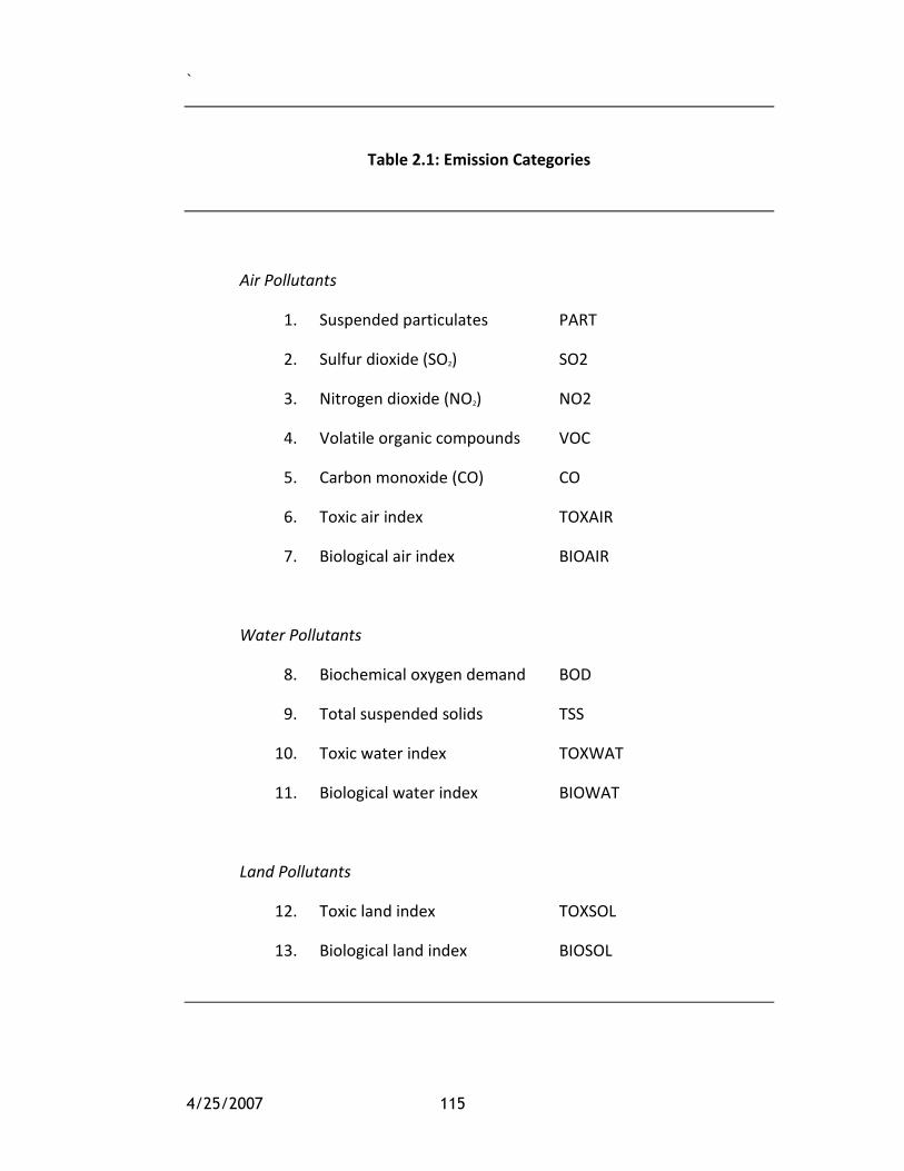
4/25/2007 115

Table 2.1: Emission Categories

Air Pollutants

1. Suspended particulates PART

2. Sulfur dioxide (SO2) SO2

3. Nitrogen dioxide (NO2) NO2

4. Volatile organic compounds VOC

5. Carbon monoxide (CO) CO

6. Toxic air index TOXAIR

7. Biological air index BIOAIR

Water Pollutants

8. Biochemical oxygen demand BOD

9. Total suspended solids TSS

10. Toxic water index TOXWAT

11. Biological water index BIOWAT

Land Pollutants

12. Toxic land index TOXSOL

13. Biological land index BIOSOL

`

4/25/2007 116

Table A3.1: Industry Statistics for Selected States, 2002

(U.S….,Bureau 2002)

ANNEX 2 – CEMENT INDUSTRY SUPPLEMENTAL DATA

`

4/25/2007 117

Tables A3.2-3.3: Kiln Data Summary By Process Type; Kiln Data Summary By Hazardous Waste Burning Status

(Regulatory…Rulemaking, 1998)

`

4/25/2007 118

Table A3.4: Portland Cement Shipped By Producers and Importers In the United States By District

`

4/25/2007 119

Table A3.5: Portland Cement Shipments in 2004 By District and

Type of Customer

Source: Van Oss, 2004

`

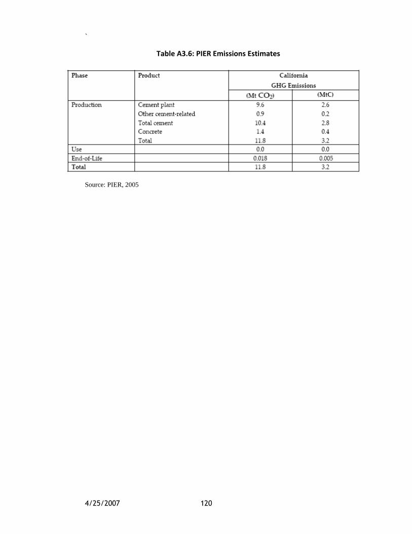
4/25/2007 120

Table A3.6: PIER Emissions Estimates

Source: PIER, 2005

`

4/25/2007 121

Table A3.7: Energy Savings Opportunities

`

4/25/2007 122

Abraham, S. (2004). "The Bush Administration's Approach to Climate Change." Science

305: 616-617.

Allergan, Inc. http://www.allergan.com/site/investors/home.asp?id=&largeText (2006)

Alza Corp. http://www.alza.com/alza/pr_1161880139 (Oct 2006)

Arc Advisory Group. http://www.arcweb.com/Events/forums/0206.htm (2006)

Babiker, M.H., J.M. Reilly, M. Mayer, R.S. Eckaus, I. Sue Wing, and R.C. Hyman

(2001). ―The MIT Emissions Prediction and Policy Analysis (EPPA) Model:

Revisions, Sensitivities, and Comparisons of Results,‖ MIT Global Change Joint

Program, Report No. 1, February.

Bayer. http://www.bayerus.com/communities/berkeley/index.html (2006) California

Energy Commission. 2004. Chemical Industry Profile.

http://energy.ca.gov/pier/iaw/industry/chemical.html Centre for the Analysis

and Dissemination of Demonstrated Energy Technologies (CADDET). 1993.

Burtraw, D., Alexander E. Farrell, Lawrence H. Goulder, and Carla Peterman (2006).

―Lessons for a Cap and Trade Program,‖ in Hanemann and Farrell (eds.)

Managing Greenhouse Gas Emissions in California, op. cit.

Burtraw, D. and K. Palmer (2004). The SO2 Cap-and-Trade Program in the United

States: A "Living Legend" of Market Effectiveness. Choosing Environmental

Policy. W. Harrington, R. D. Morgenstern and T. Sterner. Washington, DC, RFF

Press.

California Environmental Protection Agency (2006). ―Climate Action Team Report to

Governor Schwarzenegger and the Legislature,‖ March,

http://www.climatechange.ca.gov/climate_action_team/reports/2006-04-

03_FINAL_CAT_REPORT.PDF

Cement Americas. (2004). A Conversation with California Portland Cement President

and CEO James A. Repman. Retrieved Nov 27

http://cementamericas.com/mag/cement_conversation_california_portland/

7. REFERENCES

http://www.allergan.com/site/investors/home.asp?id=&largeText

http://www.alza.com/alza/pr_1161880139

http://www.arcweb.com/Events/forums/0206.htm

http://www.bayerus.com/communities/berkeley/index.html

http://energy.ca.gov/pier/iaw/industry/chemical.html

http://www.climatechange.ca.gov/climate_action_team/reports/2006-04-03_FINAL_CAT_REPORT.PDF

http://www.climatechange.ca.gov/climate_action_team/reports/2006-04-03_FINAL_CAT_REPORT.PDF

http://cementamericas.com/mag/cement_conversation_california_portland/

`

4/25/2007 123

Cemex: Cement Manufacturer Saves 2.1 Million kWh Annually with a Motor Retrofi t

Project (2005). Performance Spotlight. Retrieved on Nov 29 from

http://www.nrel.gov/docs/fy06osti/38223.pdf

Center for Clean Air Policy (2005) Reducing CO2 Emissions from California‘s Cement

Sector, October.

Center for Clean Air Policy (2005). Design of a Cap on Emissions from California Power

Demand. Washington, DC: 27.

Center For Land Use Interpretation. Retrieved Nov Dec 2 from

http://ludb.clui.org/tag/Mining/

Cheng, R., 1999. Low Emissions Burners. EETD Newsletter, Summer 1999, Lawrence

Berkeley National Laboratory, Berkeley, CA.

Coito, F., Powell, F., Worrell E., Price, L., and Friedmann R., (2005). Case Study of

the Cement Industry. Retrieved Nov 29 from

http://ies.lbl.gov/iespubs/59938.pdf

Coppinger, S. (2005) Energy Management at California Portland Cement. Retrieved on

Nov 24 from

http://www.energy.ca.gov/2005_energypolicy/documents/2005-07-

11+12_workshop/presentations/2005-07-12_COPPINGER.PDF

Cost Effective GHG Mitigation Measures for California. (2006) Summary Report: An

Independent Analysis of Measures to Reduce Greenhouse Gas Emissions in

2010 and 2020 to Meet Executive Order S-3-05. Retrieved Dec 3 from

http://www.ccap.org/domestic/Summary%20Report-Final%20_1-19-

06_.pdf

Council for Chemical Research. http://www.ccrhq.org/vision/index.html (1999)

Dunn-Edwards. http://www.dunnedwards.com/retail/content.asp?content=71 (2006)

Ellerman, A. D., P. L. Joskow, et al. (2000). Markets for Clean Air: the U.S. Acid Rain

Program. Cambridge, UK, Cambridge University Press.

Elliott, R.N., A.M. Shipley, E. Brown, R. Cleetus and S. Bernow. 2003. State-level

Analysis of Industrial Energy Use. Proc. 2003 ACEEE Summer Study on Energy

Efficiency in Industry, pp.6- 76-85, Washington, DC: ACEEE.

http://www.nrel.gov/docs/fy06osti/38223.pdf

http://ludb.clui.org/tag/Mining/

http://industrial-energy.lbl.gov/node/133

http://industrial-energy.lbl.gov/node/29

http://ies.lbl.gov/iespubs/59938.pdf

http://www.energy.ca.gov/2005_energypolicy/documents/2005-07-%0911+12_workshop/presentations/2005-07-12_COPPINGER.PDF

http://www.energy.ca.gov/2005_energypolicy/documents/2005-07-%0911+12_workshop/presentations/2005-07-12_COPPINGER.PDF

http://www.ccap.org/domestic/Summary%20Report-Final%20_1-19-06_.pdf

http://www.ccap.org/domestic/Summary%20Report-Final%20_1-19-06_.pdf

http://www.ccrhq.org/vision/index.html

http://www.dunnedwards.com/retail/content.asp?content=71

`

4/25/2007 124

Encyclopedia of American Industries Fourth Edition: Volume 1 Manufacturng Industries.

Editor Lynn M. Pearce. Thomson Gale: New York, New York

Energy Technology Support Unit (ETSU). 1999. ―Design and operation of energy-

efficient batch processes.‖ Report of the UK Best Practice Program, ETSU:

Harwell, United Kingdom

Farrell, A. E. and L. B. Lave (2004). "Emission Trading and Human Health." Annual

Review of Public Health 25: 119-138.

Fischer, C. and A. Fox (2004). Output-Based Allocations of Emissions Permits:

Efficiency and Distributional Effects in a General Equilibrium Setting with Taxes

and Trade. Washington, DC, Resources For the Future.

Fischer, C., I. W. H. Parry, et al. (2003). "Instrument choice for environmental

protection when technological innovation is endogenous." Journal of

Environmental Economics and Management 45(3): 523-545.

Genentech, Inc. http://www.gene.com/gene/ir/downloadDoc.do?id=2801 pp.7, 10

(2005)

Hanemann, W. Michael, and A.E. Farrell (eds.) (2006) ―Managing Greenhouse Gas

Emissions in California,‖ California Climate Change Center, University of

California, Berkeley, January,

http://calclimate.berkeley.edu/managing_GHGs_in_CA.html

Hanle, Lisa J. (2004). CO2 Emissions Profile of the U.S. Cement Industry. Retrieved Nov

28 from http://www.epa.gov/ttn/chief/conference/ei13/ghg/hanle.pdf)

Hanson, D. and J.A. Laitner (2004). ―An integrated analysis of policies that increase

investments in advanced-energy efficient/low carbon policies.‖ Energy

Economics 26: 739-755.

Harrison, K. and W. Antweiler (2003). "Incentives for pollution abatement: Regulation,

regulatory threats, and non-governmental pressures." Journal of Policy Analysis

and Management 22(3): 361-382.

Helme, Ned, Tom Peterson, and Eric Williams (2004). ―Allowance Allocation: Who wins

and loses under a carbon dioxide control program?‖ Center for Clean Air Policy,

http://www.ccap.org/pdf/CRA_Background_Paper.pdf

http://www.gene.com/gene/ir/downloadDoc.do?id=2801

http://calclimate.berkeley.edu/managing_GHGs_in_CA.html

http://www.epa.gov/ttn/chief/conference/ei13/ghg/hanle.pdf

`

4/25/2007 125

Hoffert, M., K. Caldeira, et al. (1998). "Energy Implications of future stabilization of

atmospheric CO2 content." Nature 395(6075): 881-884.

J.A. Laitner (2006). ―An Annotated Review of 30 Studies Describing the

Macroeconomic Impacts of State-Level Scenarios Which Promote Energy

Efficiency and Renewable Energy Technology Investments.‖ American Council

for an Energy Efficiency Economy: Comment Draft (July).

Kartha, S., M. Lazarus, et al. (2004). "Baseline recommendations for greenhouse gas

mitigation projects in the electric power sector." Energy Policy 32(4): 545-566.

Kemp, I.C. and A.W. Deakin. 1989. ―The Cascade Analysis for Energy and Process

Integration of Batch Processes, Part 3: A Case Study.‖ Chemical Engineering

Research and Design. pp.517-525.

Kerr, S. and R. G. Newell (2003). "Policy-induced technology adoption: Evidence from

the US lead phase down." Journal of Industrial Economics 51(3): 317-343.

Lifescan, Inc. http://www.lifescan.com/company/about/environment/(2006)

Linnhoff, B. 1993. Pinch Analysis: A State-of-the-Art Overview. Chemical Engineering

(AS): pp.503-522.

Marsland. 1992. A User Guide on Process Integration for the Efficient Use of Energy

(1992 edition), Institution of Chemical Engineers, Rugby, UK.

Milliman, S. R. and R. Prince (1989). "Firm Incentives to Promote Technological-Change

in Pollution-Control." Journal of Environmental Economics and Management

17(3): 247-265.

Montero, J. P. (1999). "Voluntary compliance with market-based environmental policy:

Evidence from the US Acid Rain Program." Journal of Political Economy 107(5):

998-1033.

Norberg-Bohm, V. (1999). "Stimulating 'green' technological innovation: An analysis of

alternative policy mechanisms." Policy Sciences 32(1): 13-38.

Nordhaus, R. R. and K. W. Danish (2003). Designing a mandatory greenhouse gas

reduction program for the U.S. Arlington, VA, Pew Center on Global Climate

Change: 66.

http://www.lifescan.com/company/about/environment/

`

4/25/2007 126

Ono, T. (2002). "The effects of emission permits on growth and the environment."

Environmental & Resource Economics 21(1): 75-87.

Palmer, K., D. Burtraw, et al. (2005). In Search of Simple Rules for Using CO2

Allowances to Compensate Firms. Washington, DC, Resources For the Future.

Pew Center on Global Climate Change(2006). ―Designing a Mandatory Greenhouse Gas

Reduction Program for the U.S.‖ http://www.pewclimate.org/global-warming-

in-depth/all_reports/mandatory_ghg_reduction_prgm/usgas_conc.cfm

Pfizer. http://www.pfizer.com/pfizer/lajolla/index.jsp (2003)

PIER Final Report (2005). Retrieved Nov 27 from

http://cacx.org/2005publications/CEC-500-2005-110/CEC-500-2005-

110-F.PDF

Popp, D. (2003). "Pollution control innovations and the Clean Air Act of 1990." Journal

of Policy Analysis and Management 22(4): 641-660.

Portland Cement Association: A (2004). US and Canadian Plant Information Summary

Reducing CO2 Emissions from California‘s Cement Sector. (2005). Retieved Dec

3 from http://www.climatechange.ca.gov/documents/2005-10-

14_CCAP_REPORTS/CCAP_REPORT_CEMENT.PDF

Regulatory Impact Analysis of Cement Kiln Dust Rulemaking. (1998) Retrieved from

http://www.epa.gov/epaoswer/other/ckd/ckd/ckdriafn.pdf

Resources for the Future, The Johns Hopkins University, and Towson University (2007)

―Economic and Energy Impacts from Maryland‘s Potential Participation in the

Regional Greenhouse Gas Initiative,‖ Study commissioned for the Maryland

Department of the Enviroment, Center for Integrative Environmental Research,

University of Maryland, College Park.

Roland-Holst, D. (2006a). Chapter 2: Economic Assessment of some California

Greenhouse Gas Control Policies: Applications of the BEAR Model.

Retrieved on Nov 29 from

http://calclimate.berkeley.edu/2_Economic_Assessment.pdf

Roland-Holst, D. (2006b). Economic Growth and Greenhouse Gas Mitigation in

California http://calclimate.berkeley.edu/2_Economic_Assessment.pdf

http://www.pewclimate.org/global-warming-in-depth/all_reports/mandatory_ghg_reduction_prgm/usgas_conc.cfm

http://www.pewclimate.org/global-warming-in-depth/all_reports/mandatory_ghg_reduction_prgm/usgas_conc.cfm

http://www.pfizer.com/pfizer/lajolla/index.jsp

http://cacx.org/2005publications/CEC-500-2005-110/CEC-500-2005-110-F.PDF

http://cacx.org/2005publications/CEC-500-2005-110/CEC-500-2005-110-F.PDF

http://www.climatechange.ca.gov/documents/2005-10-14_CCAP_REPORTS/CCAP_REPORT_CEMENT.PDF

http://www.climatechange.ca.gov/documents/2005-10-14_CCAP_REPORTS/CCAP_REPORT_CEMENT.PDF

http://www.epa.gov/epaoswer/other/ckd/ckd/ckdriafn.pdf



`

4/25/2007 127

Roland-Holst, David (2005). ―Berkeley Energy and Resources (BEAR) Model: Technical

Documentation,‖ Department of Agricultural and Resource Economics,

University of California, Berkeley, processed.

Rubin, J. D. (1996). "A model of intertemporal emission trading, banking, and

borrowing." Journal of Environmental Economics and Management 31(3): 269-

286.

Schennach, S. M. (2000). "The economics of pollution permit banking in the context of

Title IV of the 1990 Clean Air Act Amendments." Journal of Environmental

Economics and Management 40(3): 189-210.

Stankiewicz, A.I. and J.A. Moulijn. 2000. Process Intensification: Transforming

Chemical Engineering. Chemical Engineering Progress pp. 22-34 (January

2000).

State of California Office of the Governor. Press Release.

http://gov.ca.gov/index.php?/press-release/4074/ (2006)

Stavins, Robert N. (2003). Experience with Market-Based Environmental Policy

Instruments. The Handbook of Environmental Economics. K. Goren-Maler and J.

Vincent. Amsterdam, North-Holland/Elsevier Science. 1.

Stavins, Robert N., Judson Jaffe, and Todd Schatzki (2007) ―Too Good to Be True? An

Examination of Three Economic Assessments of California Climate Change

Policy,‖ Related Publication 07-01, AEI-Brookings Joint Center for Regulatory

Studies, Washington.

Taylor, H F W (1990)Cement Chemistry, Academic Press.

Taylor, M. R., E. S. Rubin, et al. (2003). "Effect of Government Actions on

Technological Innovation for SO2 Control." Environmental Science & Technology

37(20): 4527-4534.

The Industry Report (2006). Concrete Monthly: News from the Cement and Concrete

Industries. Retrieved on Dec 1 from

http://www.concretemonthly.com/monthly/art.php?2401

http://gov.ca.gov/index.php?/press-release/4074/


`

4/25/2007 128

The Industry Report (2006). Concrete Monthly: News from the Cement and Concrete

Industries. Retrieved on Dec 1 from


Tietenberg, T. (2003). "The tradable-permits approach to protecting the commons:

Lessons for climate change." Oxford Review of Economic Policy 19(3): 400-419.

Tschudi, W., D. Sartor, and T. Xu. 2002. An Energy Efficiency Guide for use in

Cleanroom Programming. Berkeley, CA: Lawrence Berkeley National

Laboratory: Berkeley, CA (LBNL- 49223).

United States Census Bureau (2002). Cement Manufacturing 2002. Retrieved on

November 27 from http://www.census.gov/prod/ec02/ec0231i327310.pdf

United States Portland Cement Plants. (1997) PCA Summary Report. Retrieved on Nov

27 from PCA report http://www.epa.gov/ttn/atw/pcem/plantlis.pdf

US DOE-OIT, 2002b. Industrial Combustion Technology Roadmap, A Technology

Roadmap by and for the Industrial Combustion Community. Office of Industrial

Technologies, US Department of Energy, Washington, DC.

US DOE-OIT, 2002c. Rotary Burner (Project Factsheet). Office of Industrial

Technologies, US Department of Energy, Washington, DC.

US DOE-OIT. 2000. Energy and Environmental Profile of the U.S. Chemical Industry,

Office of Industrial Technologies, U.S. Department of Energy, Washington, DC.

US DOE-STI http://www.osti.gov/bridge/product.biblio.jsp?osti_id=860891 (2004)

Van Oss, Hendrik G. (2004). Cement: USGS Commodity Summary. Retrieved Dec 4

http://minerals.usgs.gov/minerals/pubs/commodity/cement/cemenmyb04.pdf

Worrell, E. and C. Galitsky. 2004. Profile of the Chemicals Industry in California –

California Industries of the Future Program. Berkeley, CA: Lawrence Berkeley

National Laboratory (LBNL-55668) (June 2004).

Worrell, E. and Galitsky, C. (2004). Energy Efficiency Improvement Opportunities for

Cement Making: An ENERGY STAR Guide for Energy and Plant Managers.

Worrell, E., D. Phylipsen, D. Einstain and N. Martin. 2000. Energy Use and Energy

Intensity of the U.S. Chemical Industry. Berkeley, CA: Lawrence Berkeley

National Laboratory (LBNL-44314).


http://www.census.gov/prod/ec02/ec0231i327310.pdf

http://www.epa.gov/ttn/atw/pcem/plantlis.pdf

http://www.osti.gov/bridge/product.biblio.jsp?osti_id=860891

http://minerals.usgs.gov/minerals/pubs/commodity/cement/cemenmyb04.pdf

`

4/25/2007 129

Worrell, E., J-W. Bode, and J. de Beer. 1997. Energy Efficient Technologies in Industry

(ATLAS project for the European Commission). Utrecht University, Utrecht, The

Netherlands.

Cap and Trade and Structural Transition in the California...

Documents

Transcript of Cap and Trade and Structural Transition in the California...