Canopy closure exerts weak controls on understory dynamics...
47
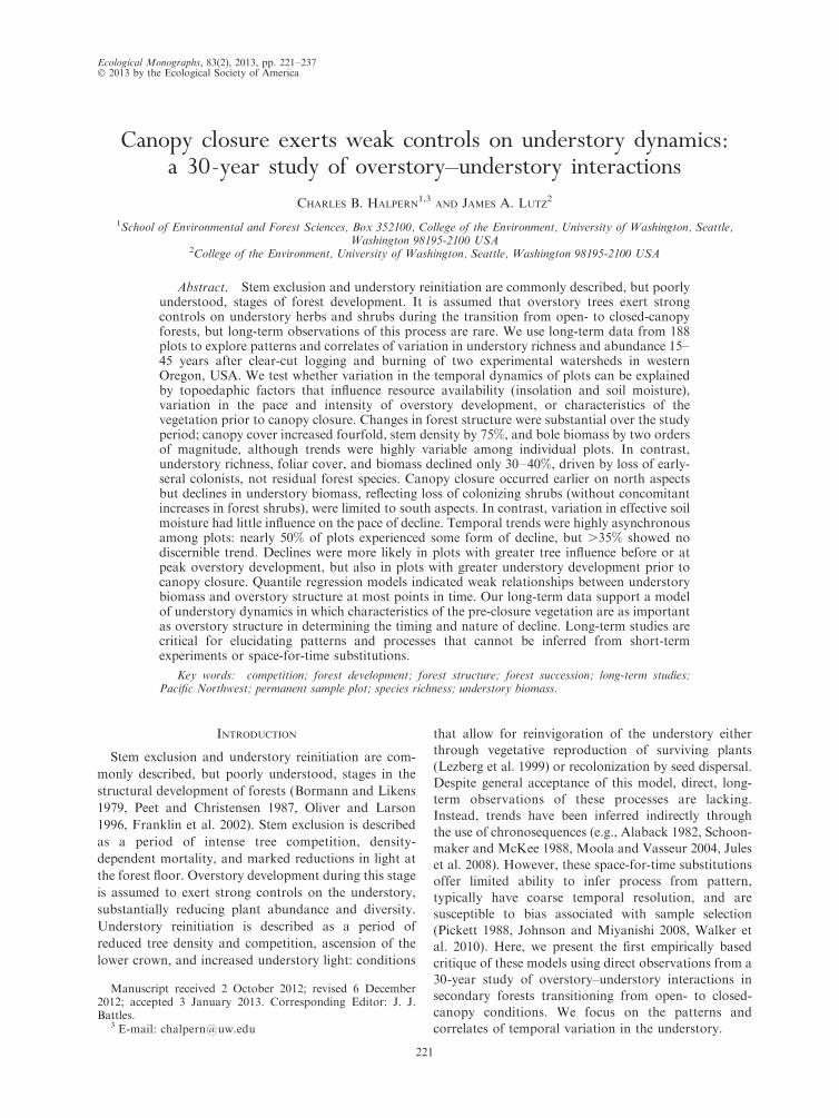
Ecological Monographs, 83(2), 2013, pp. 221–237 Ó 2013 by the Ecological Society of America Canopy closure exerts weak controls on understory dynamics: a 30-year study of overstory–understory interactions CHARLES B. HALPERN 1,3 AND JAMES A. LUTZ 2 1 School of Environmental and Forest Sciences, Box 352100, College of the Environment, University of Washington, Seattle, Washington 98195-2100 USA 2 College of the Environment, University of Washington, Seattle, Washington 98195-2100 USA Abstract. Stem exclusion and understory reinitiation are commonly described, but poorly understood, stages of forest development. It is assumed that overstory trees exert strong controls on understory herbs and shrubs during the transition from open- to closed-canopy forests, but long-term observations of this process are rare. We use long-term data from 188 plots to explore patterns and correlates of variation in understory richness and abundance 15– 45 years after clear-cut logging and burning of two experimental watersheds in western Oregon, USA. We test whether variation in the temporal dynamics of plots can be explained by topoedaphic factors that influence resource availability (insolation and soil moisture), variation in the pace and intensity of overstory development, or characteristics of the vegetation prior to canopy closure. Changes in forest structure were substantial over the study period; canopy cover increased fourfold, stem density by 75%, and bole biomass by two orders of magnitude, although trends were highly variable among individual plots. In contrast, understory richness, foliar cover, and biomass declined only 30–40%, driven by loss of early- seral colonists, not residual forest species. Canopy closure occurred earlier on north aspects but declines in understory biomass, reflecting loss of colonizing shrubs (without concomitant increases in forest shrubs), were limited to south aspects. In contrast, variation in effective soil moisture had little influence on the pace of decline. Temporal trends were highly asynchronous among plots: nearly 50% of plots experienced some form of decline, but .35% showed no discernible trend. Declines were more likely in plots with greater tree influence before or at peak overstory development, but also in plots with greater understory development prior to canopy closure. Quantile regression models indicated weak relationships between understory biomass and overstory structure at most points in time. Our long-term data support a model of understory dynamics in which characteristics of the pre-closure vegetation are as important as overstory structure in determining the timing and nature of decline. Long-term studies are critical for elucidating patterns and processes that cannot be inferred from short-term experiments or space-for-time substitutions. Key words: competition; forest development; forest structure; forest succession; long-term studies; Pacific Northwest; permanent sample plot; species richness; understory biomass. INTRODUCTION Stem exclusion and understory reinitiation are com- monly described, but poorly understood, stages in the structural development of forests (Bormann and Likens 1979, Peet and Christensen 1987, Oliver and Larson 1996, Franklin et al. 2002). Stem exclusion is described as a period of intense tree competition, density- dependent mortality, and marked reductions in light at the forest floor. Overstory development during this stage is assumed to exert strong controls on the understory, substantially reducing plant abundance and diversity. Understory reinitiation is described as a period of reduced tree density and competition, ascension of the lower crown, and increased understory light: conditions that allow for reinvigoration of the understory either through vegetative reproduction of surviving plants (Lezberg et al. 1999) or recolonization by seed dispersal. Despite general acceptance of this model, direct, long- term observations of these processes are lacking. Instead, trends have been inferred indirectly through the use of chronosequences (e.g., Alaback 1982, Schoon- maker and McKee 1988, Moola and Vasseur 2004, Jules et al. 2008). However, these space-for-time substitutions offer limited ability to infer process from pattern, typically have coarse temporal resolution, and are susceptible to bias associated with sample selection (Pickett 1988, Johnson and Miyanishi 2008, Walker et al. 2010). Here, we present the first empirically based critique of these models using direct observations from a 30-year study of overstory–understory interactions in secondary forests transitioning from open- to closed- canopy conditions. We focus on the patterns and correlates of temporal variation in the understory. Manuscript received 2 October 2012; revised 6 December 2012; accepted 3 January 2013. Corresponding Editor: J. J. Battles. 3 E-mail: [email protected] 221
Transcript of Canopy closure exerts weak controls on understory dynamics...
Ecological Monographs, 83(2), 2013, pp. 221–237� 2013 by the Ecological Society of America
Canopy closure exerts weak controls on understory dynamics:a 30-year study of overstory–understory interactions
CHARLES B. HALPERN1,3
AND JAMES A. LUTZ2
1School of Environmental and Forest Sciences, Box 352100, College of the Environment, University of Washington, Seattle,Washington 98195-2100 USA
2College of the Environment, University of Washington, Seattle, Washington 98195-2100 USA
Abstract. Stem exclusion and understory reinitiation are commonly described, but poorlyunderstood, stages of forest development. It is assumed that overstory trees exert strongcontrols on understory herbs and shrubs during the transition from open- to closed-canopyforests, but long-term observations of this process are rare. We use long-term data from 188plots to explore patterns and correlates of variation in understory richness and abundance 15–45 years after clear-cut logging and burning of two experimental watersheds in westernOregon, USA. We test whether variation in the temporal dynamics of plots can be explainedby topoedaphic factors that influence resource availability (insolation and soil moisture),variation in the pace and intensity of overstory development, or characteristics of thevegetation prior to canopy closure. Changes in forest structure were substantial over the studyperiod; canopy cover increased fourfold, stem density by 75%, and bole biomass by two ordersof magnitude, although trends were highly variable among individual plots. In contrast,understory richness, foliar cover, and biomass declined only 30–40%, driven by loss of early-seral colonists, not residual forest species. Canopy closure occurred earlier on north aspectsbut declines in understory biomass, reflecting loss of colonizing shrubs (without concomitantincreases in forest shrubs), were limited to south aspects. In contrast, variation in effective soilmoisture had little influence on the pace of decline. Temporal trends were highly asynchronousamong plots: nearly 50% of plots experienced some form of decline, but .35% showed nodiscernible trend. Declines were more likely in plots with greater tree influence before or atpeak overstory development, but also in plots with greater understory development prior tocanopy closure. Quantile regression models indicated weak relationships between understorybiomass and overstory structure at most points in time. Our long-term data support a modelof understory dynamics in which characteristics of the pre-closure vegetation are as importantas overstory structure in determining the timing and nature of decline. Long-term studies arecritical for elucidating patterns and processes that cannot be inferred from short-termexperiments or space-for-time substitutions.
Key words: competition; forest development; forest structure; forest succession; long-term studies;Pacific Northwest; permanent sample plot; species richness; understory biomass.
INTRODUCTION
Stem exclusion and understory reinitiation are com-
monly described, but poorly understood, stages in the
structural development of forests (Bormann and Likens
1979, Peet and Christensen 1987, Oliver and Larson
1996, Franklin et al. 2002). Stem exclusion is described
as a period of intense tree competition, density-
dependent mortality, and marked reductions in light at
the forest floor. Overstory development during this stage
is assumed to exert strong controls on the understory,
substantially reducing plant abundance and diversity.
Understory reinitiation is described as a period of
reduced tree density and competition, ascension of the
lower crown, and increased understory light: conditions
that allow for reinvigoration of the understory either
through vegetative reproduction of surviving plants
(Lezberg et al. 1999) or recolonization by seed dispersal.
Despite general acceptance of this model, direct, long-
term observations of these processes are lacking.
Instead, trends have been inferred indirectly through
the use of chronosequences (e.g., Alaback 1982, Schoon-
maker and McKee 1988, Moola and Vasseur 2004, Jules
et al. 2008). However, these space-for-time substitutions
offer limited ability to infer process from pattern,
typically have coarse temporal resolution, and are
susceptible to bias associated with sample selection
(Pickett 1988, Johnson and Miyanishi 2008, Walker et
al. 2010). Here, we present the first empirically based
critique of these models using direct observations from a
30-year study of overstory–understory interactions in
secondary forests transitioning from open- to closed-
canopy conditions. We focus on the patterns and
correlates of temporal variation in the understory.
Manuscript received 2 October 2012; revised 6 December2012; accepted 3 January 2013. Corresponding Editor: J. J.Battles.
3 E-mail: [email protected]
221
Several factors are likely to contribute to variation in
understory decline during canopy closure: the pace or
intensity of closure, variation in resource supply, the
extent to which trees preempt these resources, and the
ability of understory species to tolerate the conditions.
Numerous factors may influence the pace of overstory
development, including post-disturbance seed limita-
tions, resource or other environmental constraints, and
competition with early-seral vegetation (Seidel 1979,
Graham et al. 1982, Haeussler and Coates 1986, Donato
et al. 2012). Topography and soils jointly determine the
supply of light, soil moisture, and nutrients to the
understory, but trees can preempt these resources. It is
generally assumed that light is the limiting resource for
understory plants (Oliver 1981, Peet and Christensen
1988, Klinka et al. 1996). However, where soil moisture
is seasonally limiting, belowground competition with
tree roots can be intense (Coomes and Grubb 2000,
Hubbert et al. 2001). Soil trenching experiments
demonstrate that root competition from trees, which
can be acute in dense coniferous forests (Vogt et al.
1983), greatly limits productivity in the herb layer
(Tuomey and Keinholz 1931, Riegel et al. 1992, Lindh
et al. 2003).
Topoedaphic factors that influence resource availabil-
ity or mediate environmental stress can accentuate or
temper the effects of canopy closure. For example, in
topographic settings with reduced insolation (steep
north aspects), effects of canopy closure may be
accentuated, resulting in more rapid and complete loss
of the understory. On the other hand, if competition for
soil moisture is the principal constraint during closure,
effects may be tempered in sites with greater resource
supply (moist toe slopes; Montgomery et al. 2010).
Indirect effects of stress or resource variation, mediated
through patterns of stand development, are also likely.
For example, in stressful or low-productivity sites (south
aspects or dry upper slopes), rates of forest development
may be slower, delaying canopy closure. Under these
conditions, shading by trees can have positive (facilita-
tive) effects on understory development (Callaway et al.
1991, Haugo and Halpern 2010) resulting in increases,
rather than declines, in species richness and abundance.
Conversely, in more productive sites (moist toe-slopes),
the pace of forest development may be greater (Larson
et al. 2008), leading to more rapid closure of the canopy,
greater light reduction, and more dramatic declines in
the understory.
Species’ life histories and tolerances of changing
resource conditions also shape the nature of understory
development. Pre-closure communities dominated by
early-seral species with high light requirements (Grime
1977, Bazzaz 1979) should show more rapid declines in
cover and diversity than those comprising more shade-
tolerant, residual forest species. Plant size is also
relevant; short-statured herbs may decline more rapidly
than taller woody species that have greater access to
understory light. Alternatively, if plant stature and
shade tolerance are inversely related (Givnish 1982,
Thomas and Bazzaz 1999), shrubs may be moresusceptible to shading by trees (Tilman 1984, Goldberg
and Miller 1990). Timing and intensity of decline maythus depend on the representation of species with
differing functional or growth-form traits prior toclosure, which may be determined much earlier insuccession (e.g., as a function of pre-disturbance
composition or disturbance severity [Halpern 1988,Halpern and Franklin 1990, Schimmel and Granstrom
1996]).Here we use direct, long-term observations to
elucidate the influence of resource variation, overstorydevelopment, and characteristics of the pre-closure
vegetation on the dynamics of forest understories duringstem exclusion. We use data from 188 paired overstory–
understory plots in two clearcut watersheds in the H. J.Andrews Experimental Forest Long-term Ecological
Research (HJA-LTER) Site (Oregon, USA). Establishedin 1962, prior to disturbance, these plots form the basis
of the longest and most intensive study of secondarysuccession in forests of western North America (Dyrness
1973, Halpern 1988, 1989, Halpern and Franklin 1990,Halpern and Spies 1995, Lutz and Halpern 2006,
Dovciak and Halpern 2010). Steep north- and south-facing hillslopes create natural contrasts in resourceavailability (insolation and soil moisture) and environ-
mental stress that have contributed to heterogeneity inforest development (Lutz and Halpern 2006): ideal
conditions for exploring patterns and correlates ofvariation in understory dynamics during canopy closure.
We address the following questions: (1) How dounderstory richness and abundance (cover and biomass)
change during the transition from open- to closed-canopy forest? Do understory richness and abundance
converge among plots during this transition? (2) How dospecies with differing growth forms and life-history
strategies contribute to these trends? (3) Do topoedaphicfactors that influence resource availability accentuate or
temper the effects of canopy closure? (4) To what extentis understory abundance constrained by overstory
structure and do these relationships change over time?(5) How variable are individual plots in their temporaldynamics? Can this variation be explained by resource
environments, patterns of overstory development, orvegetation characteristics prior to canopy closure?
STUDY AREA
Physical environment, vegetation, and disturbance history
Watersheds 1 and 3 (WS1 and WS3) occur at low tomoderate elevations (442–1082 m) in the HJA-LTER, 80
km east of Eugene, Oregon (WS1, 44.20478 N, 122.24898
W; WS3, 44.21388 N, 122.23218 W). Both are ;100-ha
basins characteristic of the western Cascade Range. Theprimary stream channels flow southeast to northwest,creating steep north- and south-facing hillslopes (Fig. 1).
Soils are shallow to moderately deep, originating fromandesites, tuffs, breccias, and basalt flows (Rothacher et
CHARLES B. HALPERN AND JAMES A. LUTZ222 Ecological MonographsVol. 83, No. 2

al. 1967). They are moderately productive (site class II–
IV; King 1966), varying with depth and topographic
position (A. Mckee, personal communication). Textures
are mostly loamy and porosity and water-storage
capacity are generally high (Dyrness 1969).
The climate is maritime with mild, wet winters and
warm, dry summers. For 1971–2000, mean minimum
temperatures at 430 m were�1.38C (January) and mean
maxima were 28.68C (July). Annual precipitation
averages ;2200 mm (falling mostly as rain), but only
6% occurs between June and August leading to frequent
summer drought (Bierlmaier and McKee 1989; data
available online).4 Vegetation is characteristic of the
Tsuga heterophylla zone (Franklin and Dyrness 1988).
Prior to harvest, forests were dominated by mature
(125–300 years old) and old-growth (300–500 years old)
Pseudotsuga menziesii and Tsuga heterophylla with a
diversity of shade-tolerant conifers and hardwoods in
the subcanopy (Lutz and Halpern 2006). Understory
composition reflected strong topoedaphic controls on
soil moisture availability, the principal resource gradient
structuring understory composition in these forests
(Dyrness et al. 1974, Zobel et al. 1976, Hemstrom et
al. 1987). Six communities were defined along this
gradient, from dry ridgetops with shallow soils to moist
toe-slopes with deeper soils: Corylus cornuta/Gaultheria
shallon, Rhododendron macrophyllum/Gaultheria shallon,
Acer circinatum/Gaultheria shallon, Acer circinatum/
Berberis nervosa, Coptis laciniata, and Polystichum
munitum (Rothacher et al. 1967; see also Dyrness 1973,
Halpern 1988, 1989).
WS1 was clearcut over the period 1962–1966; a
skyline cable was used to transport logs to a landing
at the base of the watershed. Slash was broadcast burned
in fall 1966. WS3 was partially clearcut in 1962–1963
creating three 5–11 ha harvest units; high-lead cables
were used to transport logs to roadside landings. Slash
was broadcast burned in fall 1963. Attempts at
reforestation included aerial seeding or planting of
Pseudotsuga menziesii, but seed germination and surviv-
al were low. Thus, most regeneration has occurred
through natural seed dispersal from adjacent forests or
stump sprouting of hardwoods (Lutz and Halpern
2006).
METHODS
Field sampling
Prior to disturbance (1962), permanent understory
plots (23 2 m, slope corrected) were established at 30.5-
m intervals along multiple transects in both watersheds
(132 plots on six transects in WS1, 62 plots on 10
transects in WS3). Plots were assessed for slope and
aspect and assigned to one of the six plant communities
(Rothacher et al. 1967, Dyrness 1973). In 1979 and 1980
(14–16 years after burning), circular overstory plots (250
m2; 8.92 m radius) were established over each understory
plot (one corner of the latter served as plot center).
Understory and overstory plots were sampled at 2–6
year intervals, but not in the same year (typically one
year apart; Table 1). Six of the initial plots were dropped
from the analysis because one or more samples were
missed, yielding a total of 188 plots (129 in WS1; 59 in
WS3).
At each understory sampling date we estimated
canopy cover (%) of all vascular plant species (herbs,
tall shrubs, and trees). Several taxa that were difficult to
distinguish were combined at the genus level (Appendix
A). For tall shrubs (and most ferns) rooted in each plot,
we also measured the basal diameter of each stem (or
frond length), from which we estimated aboveground
biomass (henceforth, biomass; see Methods: Plot and
species classification and data reduction). At each
overstory sampling date, all conifers �1.4 m tall were
tagged (if not previously tagged), measured for diame-
ter, and recorded as live or dead. Conifers with breast
height diameter (dbh) .2 cm were measured at dbh;
FIG. 1. Aerial view of Watershed 1 (WS1), H. J. AndrewsExperimental Forest-LTER, Oregon, USA, taken in 1988, 22years after disturbance. The steep terrain is characteristic of thewestern Cascade Range. The primary stream channel flowseast-southeast (1108) to west-northwest (2908), creating a strongcontrast in aspect between the principal hillslopes. Photo credit:USDA Forest Service.
4 http://andrewsforest.oregonstate.edu/data/abstract.cfm?dbcode¼MS001
May 2013 223UNDERSTORY DYNAMICS DURING CANOPY CLOSURE

smaller trees were measured at the base (dba). Hard-
woods, typically stump sprouts, were either tagged and
measured at dbh (stems �5 cm dbh) or tallied by
diameter class (,3 and 3–4.9 cm). For details, see Lutz
and Halpern (2006).
Plot and species classifications and data reduction
Data from the two watersheds were combined for
analysis because physical environments and vegetation
were similar and our emphasis is on overstory–
understory interactions. The dates of logging and
burning differed between watersheds; thus we express
time as ‘‘time since disturbance’’ (years after broadcast
burning). Measurements made in the same year in
different watersheds thus represent an average time since
disturbance (Table 1). Understory plots (including tree
cover) were sampled nine times and overstory plots (tree
diameters), seven times. For analyses of overstory–
understory relationships we used the seven closest
temporal pairings of the data (difference of �1 yr;
Table 1).
To explore the influence of resource supply on
understory trends (question 3), plots were assigned to
contrasting resource environments (insolation and
effective soil moisture) as follows. Plots on opposing
hillslopes (Fig. 1) were assigned to contrasting light
environments: north (N) aspects (northwest to north-
east; n ¼ 83) and south (S) aspects (southwest to
southeast; n ¼ 57). Plots with east or west aspects (n ¼48) were not considered for this comparison. Using pre-
disturbance plant community type as an indicator of soil
moisture availability (Rothacher et al. 1967, Dyrness
1973, Zobel et al. 1976) we assigned plots to one of three
distinct site types: xeric (Corylus cornuta/Gaultheria
shallon and Rhododendron macrophyllum/Gaultheria
shallon types; n¼ 44); mesic (Acer circinatum/Gaultheria
shallon, Acer circinatum/Berberis nervosa, and Coptis
laciniata types; n¼ 97); and moist (Polystichum munitum
type; n ¼ 47).
Each taxon was assigned to a growth form (herba-
ceous or tall shrub) and life-history strategy (seral
group: colonist or residual forest species) based on
previous classifications (Dyrness 1973, Halpern and
Franklin 1990, Halpern and Spies 1995, Dovciak and
Halpern 2010; Appendix A). Forest species were those
present prior to disturbance; colonists established
thereafter. Several taxa could not be assigned to a seral
group and were omitted from analyses of seral-group
responses; however, these contributed minimally to
understory richness or abundance. Plant nomenclature
follows Hitchcock and Cronquist (1973).
Biomass was estimated using species-specific allome-
tric equations developed in or adjacent to HJA-LTER
(Gholz et al. 1979, Means et al. 1994, Halpern et al.
1996) (Appendix D). For most herbaceous species,
biomass was predicted from cover (or for ferns, from
stem basal diameter or frond length). For tall shrubs,
biomass was predicted from basal diameter. Where
equations did not exist, we substituted equations of
species of similar growth form (Appendix D). For trees,
estimates of bole biomass (live and dead) were based on
equations of Means et al. (1994) with modifications as
described by Lutz and Halpern (2006).
Analyses
Trends in overstory structure.—For each overstory
plot 3 sampling time (time since disturbance), we
computed three measures of overstory structure that
served as proxies for resource preemption: total
(summed) cover of tree species (maximum .100%), tree
density (stems/ha), and bole biomass (Mg/ha). We
computed means for the full set of plots (n ¼ 188) and
for plots representing contrasting resource environments
(N vs. S aspects and xeric, mesic, or moist sites).
Trends and variation in understory richness, cover, and
biomass.—For each understory plot3 sampling time we
computed species richness (species/plot), total cover
(maximum .100%), and biomass (Mg/ha) for the full
community and each growth form3 seral group. Means
and variation (SD and CV) were computed for the full
set of plots (questions 1 and 2). Means (and SEs) were
also computed for plots representing each resource
TABLE 1. Dates of sampling of understory and overstory plots on Watersheds 1 and 3 (WS1 and WS3) and their relationships totime since disturbance.
Understory OverstoryTime since
disturbance (yr)�Date WS1 (yr) WS3 (yr) Ave. (yr)� Date WS1 (yr) WS3 (yr) Ave. (yr)�
1979 13 16 14.51980–1981§ 14 18 16.0 1979–1980} 14 16 15 15.5
1983 17 20 18.5 1984 18 21 19.5 19.01987 21 24 22.5 1988 22 25 23.5 23.01990 24 27 25.5 1991 25 28 26.5 26.01994 28 31 29.5 1995 29 32 30.5 30.01997 31 34 32.52002 36 39 37.5 2001 35 38 36.5 37.02008 42 45 43.5 2007 41 44 42.5 43.0
� Time since disturbance averaged between watersheds.� Time since disturbance averaged for understory and overstory plots.§ Understory was sampled in 1980 in WS1 and in 1981 in WS3.} Overstory was sampled in 1980 in WS1 and in 1979 in WS3.
CHARLES B. HALPERN AND JAMES A. LUTZ224 Ecological MonographsVol. 83, No. 2
environment. We then assessed whether rates of change
over time (regression slopes) differed among resource
environments (question 3). To do so, we used general-
ized linear models to test the environment 3 time
interaction; significant interactions were followed by
pairwise comparisons of slopes. We also tested whether
individual or pooled slopes (as appropriate) differed
from zero. Although temporal trends for a small number
of variable 3 environment combinations were hump
shaped, use of linear models to approximate change over
the study period did not alter our interpretations. We
did not test whether intercepts differed among resource
environments because these represented differences that
predated effects of closure. Regression analyses were
conducted within the glm module of SPSS version 14
(SPSS 2005).
Overstory–understory relationships.—To test relation-
ships between overstory structure and understory
abundance (question 4), we used constraint-line analysis
or quantile regression, which is based on the upper
quantile of a distribution (Guo et al. 1998, Scharf et al.
1998, Cade et al. 1999). This method of modeling
‘‘maximum’’ (rather than mean) response is useful for
isolating the effect of a hypothesized constraint (e.g.,
tree cover or density) on a response variable (e.g.,
understory biomass) when there are additional unmea-
sured factors that can contribute to the response. We
used linear quantile regression (Cade and Noon 2003) to
explore relationships between maximum understory
biomass and each measure of overstory structure (tree
cover, density, and bole biomass). Given strong con-
trasts in structural development on N and S aspects, we
tested relationships separately for each aspect. We also
tested whether relationships changed over time, using
separate models for each temporal pairing of overstory–
understory data (Table 1). Emergence of a significant
relationship or a change in slope over time could reflect
a shift in the distribution of a constraining variable (e.g.,
toward greater values of tree cover, density, or bole
biomass) or a cumulative effect over time. To assess the
sensitivity of these relationships to selection of the upper
quantile (s), we compared three quantiles, s¼ 0.80, 0.90,
and 0.95. Analyses were performed in R version 2.14.1
(R Development Core Team 2011) using the quantreg
package version 4.44 (available online).5
Variation in and predictors of temporal trends.—
Temporal trends in understory abundance varied
substantially among plots, ranging from decline and
reinitiation (or not), to no change, to a continuous
increase with time. To characterize the diversity and
frequency of these temporal patterns (question 5), we fit
trends in understory abundance (cover and biomass) in
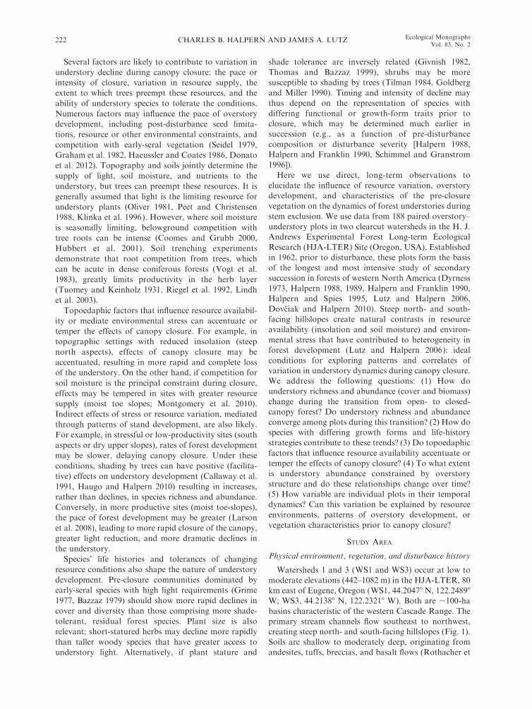
each plot to one of six model types (Fig. 2). Four of
these models captured differences in the onset or rate of
decline (or reinitiation); these were termed ‘‘reinitiating,’’
‘‘crashing,’’ ‘‘declining,’’ or ‘‘peaking’’ (the latter, typi-
cally declining only at the last measurement) (Fig. 2).
The two remaining models represented instances of no
decline and were termed ‘‘stabilizing’’ or ‘‘increasing.’’ A
model was accepted as significant at a¼ 0.05. If multiple
models were accepted for a plot, we identified the ‘‘best-
fit’’ model as that with greatest adjusted R2.
We then used multinomial logistic regression (MLR;
Hosmer and Lemeshow 1989, Trexler and Travis 1993) to
test whether plots with similar temporal trends (based on
best-fit models) shared similar characteristics, i.e., re-
source environments, patterns of structural development,
or vegetation characteristics prior to canopy closure
(question 5). MLR is useful for identifying variables
(categorical or continuous predictors), that differentiate
among multiple outcomes, in this case, model types.
Separate regressions were run for understory cover and
biomass. We tested multiple predictors of six general
types: (1) resource environments (N vs. S aspects; xeric,
mesic, or moist sites); (2) pre-closure tree influence (tree
cover, density, or bole biomass at 14–16 yr); (3) rate of
overstory development (timing of minimum or maximum
tree cover, density, or bole biomass); (4) intensity of
overstory development (minimum or maximum tree
cover, density, or bole biomass); (5) post-closure distur-
bance (bole biomass lost to mechanical disturbance, a
proxy for increased resource availability (Lutz and
Halpern 2006); and (6) seral group abundance prior to
canopy closure (cover or biomass of colonizing and
residual forest species). Due to the small sample sizes of
several model types, some plots were reclassified to the
next best-fitting model and regressions were run on fewer
model types. Specifically, for cover, plots modeled as
‘‘stabilizing’’ (n ¼ 3) were reclassified, resulting in five
model types. For biomass, plots classified as ‘‘declining’’
(n ¼ 12), ‘‘stabilizing’’ (n ¼ 1), and ‘‘increasing’’ (n ¼ 11)
were reclassified, resulting in three model types: ‘‘reini-
FIG. 2. Schematic representation of the six model types towhich temporal trends in plot abundance (cover or biomass)were fit. Black and gray lines illustrate variation in themagnitude or rate of change in abundance within a modeltype. Models represent plots that differed in the pace or timingof decline (upper row) or that showed a delay in, or no effect of,canopy closure (bottom row).
5 http://cran.r-project.org/web/packages/quantreg/index.html
May 2013 225UNDERSTORY DYNAMICS DURING CANOPY CLOSURE
tiating,’’ ‘‘crashing,’’ and ‘‘peaking.’’ For each regression,
the set of plots showing no temporal trend was chosen as
the reference category (required in MLR), allowing each
of the final model types to be compared with a common
‘‘null’’ model. The significance of predictors was deter-
mined stepwise, using the likelihood ratio as a removal
test with a ¼ 0.05. Analyses were conducted in SPSS
version 14 (SPSS 2005).
RESULTS
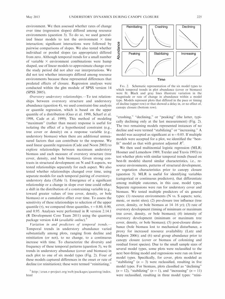
Trends in forest structure
Total tree cover increased continuously (Fig. 3a), with
80% of plots reaching �100% cover within the 30 years
of study. Closure occurred earlier on N aspects (.100%cover at ;25 yr) than on S aspects (peak cover of 86% at
;32 yr; Fig. 3b). Cover was consistently greater in
moist- than in mesic- or xeric-site communities (Fig. 3c).
Tree density peaked much earlier (;22 yr; Fig. 3d) than
did cover, with 75% of plots reaching maximum density
within ;25 years. Maximum density on N aspects was
more than twice that on S aspects (;4900 vs. 2300 trees/
ha), but subsequent declines were steeper (Fig. 3e). Peak
densities tended to be greater in moist- than in mesic- or
xeric-site communities, but these differences were small
(Fig. 3f ). Bole biomass increased continuously (Fig. 3g).
Biomass was greater on N than on S aspects for most of
the study period (Fig. 3h), but was similar among
moist-, mesic-, and xeric-site communities until the final
measurement (Fig. 3i ).
Trends and variation in understory richness, cover,
and biomass
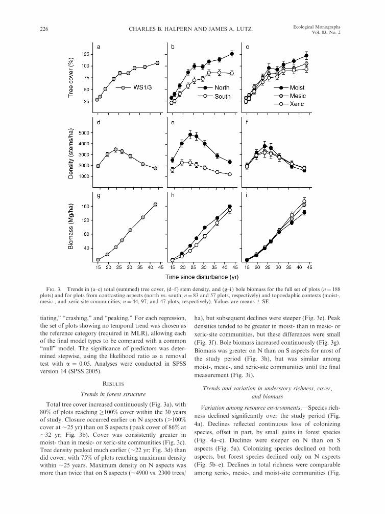
Variation among resource environments.—Species rich-
ness declined significantly over the study period (Fig.
4a). Declines reflected continuous loss of colonizing
species, offset in part, by small gains in forest species
(Fig. 4a–c). Declines were steeper on N than on S
aspects (Fig. 5a). Colonizing species declined on both
aspects, but forest species declined only on N aspects
(Fig. 5b–e). Declines in total richness were comparable
among xeric-, mesic-, and moist-site communities (Fig.
FIG. 3. Trends in (a–c) total (summed) tree cover, (d–f ) stem density, and (g–i) bole biomass for the full set of plots (n¼ 188plots) and for plots from contrasting aspects (north vs. south; n¼ 83 and 57 plots, respectively) and topoedaphic contexts (moist-,mesic-, and xeric-site communities; n ¼ 44, 97, and 47 plots, respectively). Values are means 6 SE.
CHARLES B. HALPERN AND JAMES A. LUTZ226 Ecological MonographsVol. 83, No. 2

5f ), but for colonizing herbs they were steepest in moistsites (Fig. 5i ).
Total understory cover declined earlier and at a
steeper rate than did richness. Nevertheless, mean cover
did not fall below ;80% (Fig. 4d). Declines reflected loss
of the dominant colonizing shrubs (Ceanothus sangui-
neus, C. velutinus, Rubus parviflorus), and herbs (Epi-
lobium angustifolium). In contrast, cover of forest shrubs(mainly Acer circinatum) increased (Fig. 4e). Declines
were comparable on N and S aspects for all plant groups
except forest shrubs, which showed no change on N
aspects but continuous increase on S aspects (Fig. 6c).
Declines (or increases in forest shrubs; Fig. 6h) were also
comparable among moist-, mesic-, and xeric-site com-munities.
Understory biomass, dominated by shrubs, declined
less steeply than did cover (Fig. 4g). Similar to trends in
cover, colonizing shrubs (primarily Ceanothus spp.)
declined and forest shrubs (primarily Acer circinatum)
increased (Fig. 4h). Declines in total biomass were
significant on S aspects, where colonists dominated the
pre-closure vegetations (Fig. 7a–c). However, there wasno net change on N aspects: declines in colonists were
balanced by increases in forest shrubs (Fig. 7a–c). Total
biomass declined more steeply in xeric- than in mesic- or
moist-site communities (Fig. 7f ). Declines in colonizing
shrubs were comparable among site types (Fig. 7g), but
rates of increase among forest shrubs differed (greatestfor mesic-site communities; Fig. 7h).
Plot-scale variation.—Individual plots exhibited abroad range of variation (one to two orders of
magnitude) in total understory richness, cover, and
biomass (Fig. 8a–c). Variation in richness and cover
changed little or declined slowly, but variation in
biomass increased markedly over time (Fig. 8d, e).
Overstory–understory relationships
Quantile regression models indicated weak relation-
ships between maximum understory biomass and
overstory structure (Fig. 9). Although understory
biomass tended to decline with tree cover, density, and
bole biomass, few models produced significant relation-
FIG. 4. Trends in (a–c) understory richness (species/plot), (d–f ) total (summed) cover, and (g–i) biomass for the full set of plots(n¼ 188 plots), including the contributions of colonizing and residual forest species. Understory totals (left column) are partitionedby growth form (middle and right columns). Values are means 6 SE.
May 2013 227UNDERSTORY DYNAMICS DURING CANOPY CLOSURE
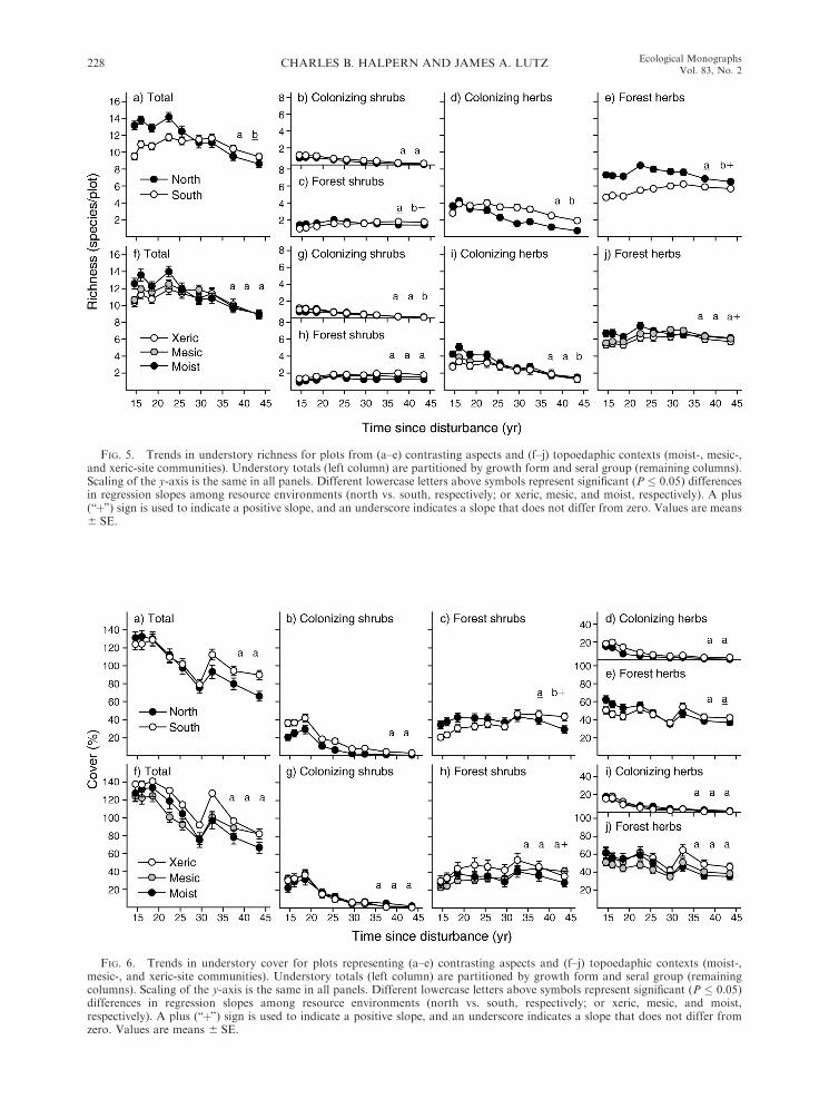
FIG. 5. Trends in understory richness for plots from (a–e) contrasting aspects and (f–j) topoedaphic contexts (moist-, mesic-,and xeric-site communities). Understory totals (left column) are partitioned by growth form and seral group (remaining columns).Scaling of the y-axis is the same in all panels. Different lowercase letters above symbols represent significant (P � 0.05) differencesin regression slopes among resource environments (north vs. south, respectively; or xeric, mesic, and moist, respectively). A plus(‘‘þ’’) sign is used to indicate a positive slope, and an underscore indicates a slope that does not differ from zero. Values are means6 SE.
FIG. 6. Trends in understory cover for plots representing (a–e) contrasting aspects and (f–j) topoedaphic contexts (moist-,mesic-, and xeric-site communities). Understory totals (left column) are partitioned by growth form and seral group (remainingcolumns). Scaling of the y-axis is the same in all panels. Different lowercase letters above symbols represent significant (P � 0.05)differences in regression slopes among resource environments (north vs. south, respectively; or xeric, mesic, and moist,respectively). A plus (‘‘þ’’) sign is used to indicate a positive slope, and an underscore indicates a slope that does not differ fromzero. Values are means 6 SE.
CHARLES B. HALPERN AND JAMES A. LUTZ228 Ecological MonographsVol. 83, No. 2

ships for any of the upper quantiles tested: five of 42
models (overstory–understory combinations 3 times) at
s ¼ 0.80, three at s ¼ 0.90, and four s ¼ 0.95. Most of
these occurred early in stand development (�19 yr),
prior to peak density or canopy cover.
Variation in and predictors of temporal trends
For most plots, temporal trends in understory
abundance conformed to one or more of the six model
types (Fig. 2, Table 2). Trends in cover could be modeled
for 117 plots (62%) and trends in biomass for 123 plots
(65%). Trends could not be modeled in 35–38% of plots.
The most frequent model types were reinitiating,
crashing, and declining (71–87 plots; 38–46%). The
most frequent best-fit model for cover was reinitiating
(51 plots, 27%) and, for biomass, it was crashing (45
plots, 24%). Trends less often conformed to peaking,
stabilizing, or increasing forms (1–21 plots; ,1–11%).
Multinomial logistic regression models were highly
significant (P , 0.001), successfully differentiating
among model types (Tables 3 and 4). For trends in
cover, significant predictors included topoedaphic con-
text (soil moisture availability, P¼0.02), pre-closure tree
cover (P , 0.001) and density (P ¼ 0.006), and pre-
closure understory development (cover of colonizing
and forest species, P , 0.001 and P ¼ 0.001; Table 3).
Relative to the reference group (no temporal trend),
plots that declined in cover (reinitiating, crashing,
declining, or peaking) had significantly greater tree
influence (cover or density) prior to closure and, for all
but the peaking group, significantly greater understory
development (cover of colonizing or forest species; see
parameter mean values in Table 3). Plots in the peaking
group were much more likely to be xeric site commu-
nities and less often mesic site communities. Plots in
which cover did not decline (increasing) had limited
understory development prior to closure.
For trends in biomass (reduced to three model types;
Table 4), significant predictors included timing and
intensity of overstory development (timing of maximum
tree density and cover, P , 0.001 and P¼ 0.02) and pre-
closure understory development (biomass of colonizing
and forest species, P , 0.001 and P¼ 0.003). All model
types attained maximum tree density earlier than the
reference group (see parameter mean values in Table 4).
Plots characterized by earlier or more rapid declines
(reinitiating and crashing) had greater biomass of
colonizing species prior to canopy closure. Plots in
which declines occurred later (peaking), had significant-
ly greater biomass of forest species. Surprisingly, plots
that experienced significant (30–50%) loss of overstory
biomass to gap-forming disturbance (Lutz and Halpern
2006) did not share similar responses.
DISCUSSION
Conventional models of early forest development
describe the stem-exclusion phase as one of intense tree
competition, low light at the forest floor, and dramatic
declines in the abundance and diversity of understory
plants (Bormann and Likens 1979, Peet and Christensen
FIG. 7. Trends in understory biomass for plots representing (a–e) contrasting aspects and (f–j) topoedaphic contexts (moist-,mesic-, and xeric-site communities). Understory totals (left column) are partitioned by growth form and seral group (remainingcolumns). Scaling of the y-axis is the same in all panels. Different lowercase letters above symbols represent significant (P � 0.05)differences in regression slopes among resource environments (north vs. south, respectively; or xeric, mesic, and moist,respectively). A plus (‘‘þ’’) sign is used to indicate a positive slope, and an underscore indicates a slope that does not differ fromzero. Values are means 6 SE.
May 2013 229UNDERSTORY DYNAMICS DURING CANOPY CLOSURE

1987, Oliver and Larson 1996). Our permanent-plot
observations, even when aggregated at larger spatial
scales (comparable to those implicit in conventional
models), illustrate much less dramatic declines in the
abundance and diversity of the understory. Recent
criticisms and elaborations of these models emphasize
their simplicity and limited relevance to the broader
range of pathways initiated by natural disturbances. In
particular, they fail to acknowledge the potential for
delayed or incomplete closure of the canopy (Franklin et
al. 2002, Donato et al. 2012). Our long-term studies
provide a rich and detailed picture of this variation and,
more importantly, that it can arise from a common
(single) disturbance (see also Halpern 1988).
General trends in overstory and understory characteristics
Forest structure changed significantly over the three
decades of study (15–45 yr after disturbance). Canopy
cover increased fourfold (25% to .100%), tree density
nearly doubled to ;3500 stems/ha then declined
comparably, and biomass accumulated linearly (from 7
to 160 Mg/ha; also see Lutz and Halpern 2006).
However, changes in the understory were moderate by
comparison. Richness, cover, and biomass declined by
30–40% (;10% per decade), reflecting loss of colonizing
species that had peaked earlier in succession (Dyrness
1973, Halpern 1989, Halpern and Franklin 1990). In
contrast, residual forest species changed little (herbs) or
increased significantly (shrubs). Moreover, the small
decline in forest herbs was attributable to a small
number of ‘‘release’’ herbs (e.g., Rubus ursinus; Appen-
dix B [McKenzie et al. 2000, Lindh and Muir 2004]):
species of low initial abundance that expanded rapidly
after overstory removal (Halpern 1989). Similar declines
were not observed for the vast majority of forest species,
including old-growth dominants (Berberis nervosa,
Gaultheria shallon, and Polystichum munitum; Appendi-
ces B and C; see Plate 1). In fact, understory richness
and cover following closure were comparable to levels
observed prior to disturbance (Dyrness 1973, Halpern
and Franklin 1990). Rather than causing wholesale
suppression of the understory, stem-exclusion thus
FIG. 8. Plot-level variation in understory (a) richness, (b) cover, and (c) biomass, and associated trends in the (d) SD and (e) CVof each measure. Plots from WS1 (n¼ 129 plots) and WS3 (n¼ 59 plots) are coded separately and displaced to reduce overlap; SDand CV are based on the full set of plots (n ¼ 188 plots).
CHARLES B. HALPERN AND JAMES A. LUTZ230 Ecological MonographsVol. 83, No. 2

appears to act as a filter, selectively removing the
shade-intolerant colonists from a highly enriched post-
disturbance community.
Similar trends in understory richness and cover have
been described from a chronosequence of Pseudotsuga-
dominated stands in western Oregon, albeit for a limited
sample of post-closure sites and a much narrower range
of environments (i.e., Rhododendron/Gaultheria commu-
nity [Schoonmaker and McKee 1988]). However, trends
in biomass have not been described for this system and
make apparent how interpretations of understory
decline can differ with the metric of abundance: herbs
and shrubs contributed comparably to declines in cover,
but shrubs dominated the decline in biomass. Although
the gradual accumulation of stem wood has a tempering
effect on biomass increase in shrubs, when stems die, it
results in an abrupt and substantial loss. Our results
reinforce the idea that in physiognomically diverse
vegetation, species’ contributions to community prop-
erties are highly dependent on the measure of abundance
(Guo and Rundel 1997, Chiarucci et al. 1999).
FIG. 9. Relationships between measures of overstory structure (bole biomass, tree density, and total cover) and understorybiomass for each of the seven temporal pairings of overstory and understory plots. Quantile regression lines are shown forsignificant relationships (P � 0.05) for s¼ 0.90 (black lines) and s¼ 0.80 (gray lines); the four significant relationships for s¼ 0.95are not shown. For clarity, plots in which understory biomass exceeded 85 Mg/ha are not shown but were included in analyses (n¼1–6 per temporal sample).
May 2013 231UNDERSTORY DYNAMICS DURING CANOPY CLOSURE

Variation across resource and environmental
stress gradients
We hypothesized that topoedaphic factors thatinfluence resource availability or that mediate environ-mental stress, could temper or exacerbate rates of
understory decline, either directly through effects onresource supply (Fahey et al. 1998) or indirectly by
influencing the pace of overstory development (Larsonet al. 2008). Indeed, aspect had a dramatic effect on the
pace and intensity of overstory development, withcanopy closure occurring .10 yr earlier on N than onS aspects. Substantially greater densities of Pseudotsuga
and shade-tolerant Tsuga (Lutz and Halpern 2006) are
indicative of a less stressful regenerative environment on
N aspects (Isaac 1943, Silen 1960, Larson and Franklin
2005). Although aspect-related declines in understory
richness and cover were consistent with a model of
resource preemption (i.e., greater canopy shading or
greater root competition with trees [Coomes and Grubb
2000, Lindh et al. 2003]), the differences between aspects
were much less dramatic than those of the overstory. In
stark contrast, understory biomass declined on S, but
not N aspects. This counterintuitive result can be
explained by the spatial distribution and successional
dynamics of the principal colonists: seed banking shrubs
in the genus Ceanothus. Ceanothus spp. showed greater
development on S aspects, where warmer sites, greater
burn severity, and more open, post-disturbance condi-
tions are likely to have enhanced germination and
growth (Mueggler 1965, Hickey and Leege 1970, Orme
and Leege 1976, Noste 1985, Halpern 1989). However,
Ceanothus is sensitive to even moderate levels of shading
and has a relatively short lifespan in this system
(Mueggler 1965, Zavitkovski and Newton 1968, Conard
et al. 1985). Greater accumulation of biomass on S
aspects thus resulted in greater loss of biomass when
stems died. Because biomass and foliar cover are poorly
correlated in mature stems (C. B. Halpern, personal
observation), mortality did not have the same effect on
relative loss of cover. In sum, aspect-related declines in
understory biomass are better explained by variation in
the initial abundance of colonists than by resource
supply.
TABLE 2. Numbers of sample plots for which temporal trendsin total understory cover and biomass conformed to one ormore of six model types.
Name Model type
Cover Biomass
FitBestfit� Fit
Bestfit�
Reinitiating y ¼ y0 þ at þ bt 2; b . 0 71 51 75 33Crashing y ¼ ae�bt; b . 0 87 17 82 45Declining y ¼ y0 þ at; a , 0 86 24 73 12Peaking y ¼ y0 þ at þ bt 2; b , 0 27 15 28 21Stabilizing y ¼ a(1 – e�bt); b . 0 11 3 20 1Increasing y ¼ y0 þ at; a . 0 11 7 17 11No trend 71 65
Notes: Temporal trends were modeled for 188 plots (ninesampling dates per plot). A model was accepted as significant atan alpha of 0.05. The response variable, y, is cover or biomass;y0 is the intercept; a and b are coefficients; and t is time sincedisturbance. See Fig. 2 for the shape of curves associated witheach model type.
� Model with the highest adjusted R2 among acceptedmodels.
TABLE 3. Multinomial logistic regression coefficients and parameter mean values for predictors that differentiate among plots offive model types representing differing trends in total understory cover.
Predictors Reinitiating Crashing Declining Peaking Increasing No trend
Regression coefficients
Intercept �4.335 �5.570 �4.192 �4.878 0.632
Moisture
Moist-site community 0.942 0.927 1.137 2.156 �1.078Xeric-site communities �0.301 1.019 0.032 2.244 �0.143
Pre-closure tree cover 0.019 0.033 �0.004 �0.015 �0.004Pre-closure tree density 0.000 0.000 0.000 0.000 0.000Pre-closure colonizing species cover 0.032 0.036 0.018 0.015 �0.039Pre-closure forest species cover 0.009 0.002 0.016 0.009 �0.021
Parameter mean values
Moisture
Moist-site community (% of plots) 29.4 17.6 37.5 33.3 10.0 31.0Mesic-site communities (% of plots) 56.9 47.1 41.7 13.3 70.0 46.5Xeric-site communities (% of plots) 13.7 35.3 20.8 53.3 20.0 22.5
Pre-closure tree cover (%) 46.7 55.8 23.2 17.7 34.6 27.8Pre-closure tree density (trees/ha) 2709 1898 2072 2353 1323 1620Pre-closure colonizing species cover (%) 59.8 63.4 46.6 44.5 19.4 42.6Pre-closure forest species cover (%) 85.9 67.5 114.8 98.6 44.1 77.4
Notes: From the original classification (Table 2), the three plots modeled as ‘‘stabilizing’’ were reclassified to the next best-fittingmodel, ‘‘increasing.’’ The reference category for the regression was the set of plots whose temporal trends did not fit any of themodel types (‘‘no trend’’). Only predictors with significant contributions are shown (significant parameters [P � 0.05] are inboldface type). For a list of the full set of predictors considered, see Analyses: Variation in and predictors of temporal trends. See Fig.2 for the shape of curves associated with each model type.
CHARLES B. HALPERN AND JAMES A. LUTZ232 Ecological MonographsVol. 83, No. 2
In contrast to the response to aspect, differences in the
pace or intensity of overstory development were small
among sites with differing effective soil moisture. Trends
in stem density were remarkably similar among xeric-,
mesic-, and moist-site communities, and although moist
sites developed greater canopy cover (reflecting greater
establishment of sub-canopy Tsuga), they accumulated
less bole biomass. Similarly, there was scant evidence
that moisture supply had a moderating influence on
understory decline. Declines in richness of colonizing
herbs were steepest in moist-site communities, and
declines in total biomass were steepest in dry-site
communities, locations where colonists were either most
diverse or most abundant, respectively. Even among
residual forest shrubs that did not suffer declines during
closure, biomass trends did not correlate with proxies
for resource supply. Biomass accumulated on N but not
S aspects (despite greater insolation and reduced canopy
shading) and in mesic, but not moist or xeric site
communities. These differences in growth likely reflect
inherent compositional variation in the shrub layer:
prevalence of more shade-tolerant Acer (Russel 1974,
O’Dea et al. 1995) on N-facing and mesic sites and less
tolerant Rhododendron and Corylus on S-facing and
xeric sites.
Understory variation in time and space
We expected resource preemption during canopy
closure to reduce not only the average richness and
abundance of the understory, but also the variability
among plots, leading to convergence in community
properties (Christensen and Peet 1984). Implicit in the
models of Clements (1916), convergence during succes-
sion has been the subject of considerable theoretical and
empirical study (Margalef 1968, Facelli and D’Angela
1990, Leps 1991, Frelich and Reich 1995, Walker et al.
2010). Although it is typically viewed from the
perspective of species composition, the underlying
mechanism, interspecific interactions that sort among
species, should result in convergence of other commu-
nity properties as well (Wilson et al. 1987, Zobel et al.
1993). Here we saw limited evidence of convergence in
the richness, cover, or biomass of plots, either in the
range of values or in simple measures of variability (CV
and SD). Lack of convergence in the understory could
reflect corresponding heterogeneity in the overstory.
Indeed, variation in forest structure either remained high
(tree density) or increased over time (bole biomass; Lutz
and Halpern 2006). However, this explanation would
also imply a strong negative relationship between
overstory and understory characteristics, which was
not apparent in the broad scatter of plots used in
quantile regressions (Fig. 9). Moreover, among the few
significant models of maximum understory response,
most occurred well before peak tree density or canopy
cover. Both of these outcomes, the lack of convergence
and the quantile regression results, run counter to a
model in which understory decline is driven by overstory
influences. However, they are consistent with the
dynamics of colonizing shrubs which dominated the
decline process.
Early stand development in this system may be more
accurately described as a spatiotemporal mosaic of
vegetation states and transitions, with asynchrony
among individual forest patches (or plots) dampening
any directional trends at larger scales. Although cover
and biomass were most often modeled as reinitiating or
crashing, delays (peaking) or no evidence of decline were
also common, even after four decades, a sharp contrast
to the simple dynamics of decline described by
conventional models. The results of multinomial logistic
regression provide insights into this variation. Declines
were more likely to occur where there was greater tree
influence (cover or density) before or at peak overstory
development, and where there was greater initial cover
or biomass in the understory (thus greater potential for
decline). Not surprisingly, plots with greater biomass of
colonizing species followed ‘‘faster’’ trajectories (reini-
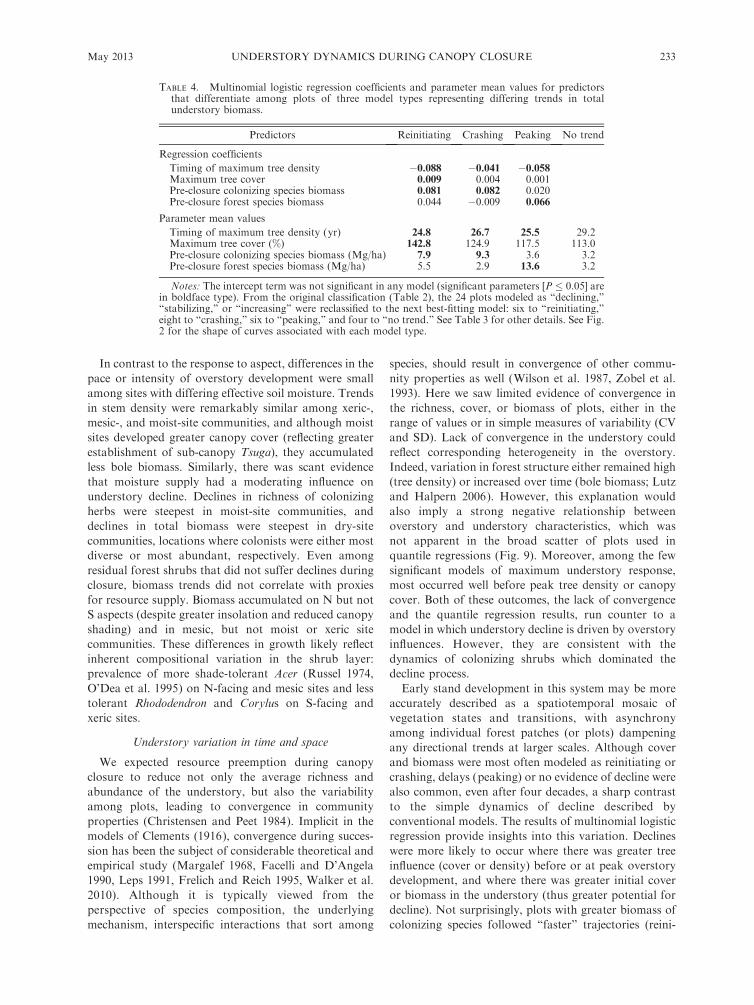
TABLE 4. Multinomial logistic regression coefficients and parameter mean values for predictorsthat differentiate among plots of three model types representing differing trends in totalunderstory biomass.
Predictors Reinitiating Crashing Peaking No trend
Regression coefficients
Timing of maximum tree density �0.088 �0.041 �0.058Maximum tree cover 0.009 0.004 0.001Pre-closure colonizing species biomass 0.081 0.082 0.020Pre-closure forest species biomass 0.044 �0.009 0.066
Parameter mean values
Timing of maximum tree density (yr) 24.8 26.7 25.5 29.2Maximum tree cover (%) 142.8 124.9 117.5 113.0Pre-closure colonizing species biomass (Mg/ha) 7.9 9.3 3.6 3.2Pre-closure forest species biomass (Mg/ha) 5.5 2.9 13.6 3.2
Notes: The intercept term was not significant in any model (significant parameters [P � 0.05] arein boldface type). From the original classification (Table 2), the 24 plots modeled as ‘‘declining,’’‘‘stabilizing,’’ or ‘‘increasing’’ were reclassified to the next best-fitting model: six to ‘‘reinitiating,’’eight to ‘‘crashing,’’ six to ‘‘peaking,’’ and four to ‘‘no trend.’’ See Table 3 for other details. See Fig.2 for the shape of curves associated with each model type.
May 2013 233UNDERSTORY DYNAMICS DURING CANOPY CLOSURE

tiating or crashing), plots with greater biomass of forest
species ‘‘slower’’ trajectories (peaking), and plots with
limited understory development either an increase or no
discernible trend. Interestingly, however, plots that lost
significant overstory biomass to gap-forming distur-
bance (Lutz and Halpern 2006) did not respond
positively (increasing or reinitiating), suggesting that
damage or burial of the understory by treefall may
balance the benefits of sudden increases in light or
belowground resources. Although gap formation early
in succession may contribute to the structural complex-
ity of older forests (Lutz and Halpern 2006, Lutz et al.
2012), it does not appear critical to reinitiation of the
understory.
The ability to link variation in post-closure dynamics
to characteristics of the pre-closure vegetation highlights
the value of long-term studies for elucidating patterns
and processes that are difficult (or impossible) to infer
with a chronosequence approach. Indeed, variation in
the characteristics of the pre-closure vegetation (e.g.,
dominance by colonizing species or relative shade-
tolerance of forest shrubs) may be as important as the
pace or intensity of overstory development. We do not
address the causes of this variation: disturbance severity
and pre-disturbance composition (described in Halpern
1988, Halpern and Franklin 1990, Halpern and Spies
1995). Rather, we emphasize that this pre-closure
variation exists and has important consequences for
the post-closure dynamics of these forests, either by
accentuating or dampening the pace of decline.
Conclusions
Although there is heuristic value to conventional,
stage-based models of stand development, their rele-
vance to forests initiated by natural disturbance has
been questioned (Franklin et al. 2002, Donato et al.
2012). It has been argued that these simple models fail to
account for the complexity of structures and diversity of
PLATE 1. Dense, post-closure stand in Watershed 1 (WS1) with a well-developed understory of Polystichum munitum. Photocredit: C. B. Halpern.
CHARLES B. HALPERN AND JAMES A. LUTZ234 Ecological MonographsVol. 83, No. 2

regeneration pathways initiated by natural stand-replac-
ing disturbances. For example, they ignore the potential
for protracted, low-density recruitment that can result in
slow or incomplete closure of the canopy (Tappeiner et
al. 1997, Franklin et al. 2002, Donato et al. 2009, 2012,
Turner et al. 2009). Although the disturbances in these
experimental watersheds were not ‘‘natural,’’ the vari-
ability of subsequent regeneration patterns clearly
supports this view (Lutz and Halpern 2006). They also
suggest a more complex model of understory develop-
ment, one in which the dynamics of the understory and
overstory are loosely coupled in space and time, and in
which the characteristics of the understory vegetation
are as important as those of the overstory in the timing
and nature of decline. Natural disturbances that create
greater diversity of live and dead structures (or
biological legacies), would likely enhance this spatial
and temporal variability. Just as structural diversity can
arise early in the development of forests in ways that
advance future complexity (Swanson et al. 2011, Donato
et al. 2012, Lutz et al. 2012), so too can diversity in the
understory. Clearly, in this system, the notion of stem-
exclusion as a temporal bottleneck in the development of
the understory does not hold. Our long-term studies of
structural and compositional change provide novel
insights into successional processes that cannot be
gained from short-term experiments or space-for-time
substitutions.
ACKNOWLEDGMENTS
We dedicate this paper to the memory of Ted Dyrness, whoestablished these plots in 1962 and, together with Al Levno,made the initial and early post-harvest measurements. Tedanticipated the value of the permanent-plot system, but perhapsnot its longevity. We thank Jerry Franklin, Art McKee, andFrederick Swanson for long-term support and encouragementof this work. Steven Acker, Richard Brainerd, Howard Bruner,and Mark Klopsch supervised data collection at various pointsduring the study. Many others assisted with data collection butare too numerous to name individually. Gody Spycher andSuzanne Remillard assisted with database management. Weappreciate the critiques of earlier drafts of the manuscript bySteven Acker, Joseph Antos, Frederick Swanson, and theanonymous reviewers. Logistical support was provided by theH. J. Andrews Experimental Forest. Funding was provided bythe USDA Forest Service PNW Research Station (01-CA-112619522-223) and the National Science Foundation (DEB8012162, BSR 8215174, BSR 8315174, BSR 8514325, DEB0218088).
LITERATURE CITED
Alaback, P. B. 1982. Dynamics of understory biomass in Sitkaspruce–western hemlock forests of southeast Alaska. Ecology63:1932–1948.
Bazzaz, F. A. 1979. Physiological ecology of plant succession.Annual Review of Ecology and Systematics 10:351–371.
Bierlmaier, F., and A. McKee. 1989. Climatic summaries anddocumentation for the primary meteorological station, H. J.Andrews Experimental Forest, 1972–1984. General TechnicalReport PNW-GTR-242. USDA Forest Service, Portland,Oregon, USA.
Bormann, F. H., and G. E. Likens. 1979. Pattern and process ina forested ecosystem. Springer, New York, New York, USA.
Cade, B. S., and B. R. Noon. 2003. A gentle introduction toquantile regression for ecologists. Frontiers in Ecology andthe Environment 1:412–420.
Cade, B. S., J. W. Terrell, and R. L. Schroeder. 1999.Estimating effects of limiting factors with regression quan-tiles. Ecology 80:311–323.
Callaway, R. M., N. M. Nadkarni, and B. E. Mahall. 1991.Facilitation and interference of Quercus douglasii on under-story productivity in central California. Ecology 72:1484–1499.
Chiarucci, A., J. B. Wilson, B. J. Anderson, and V. DeDominicis. 1999. Cover versus biomass as an estimate ofspecies abundance: Does it make a difference to theconclusions? Journal of Vegetation Science 10:35–42.
Christensen, N. L., and R. K. Peet. 1984. Convergence duringsecondary forest succession. Journal of Ecology 72:25–36.
Clements, F. E. 1916. Plant succession. Carnegie InstitutionPublication 242.
Conard, S. G., A. E. Jaramillo, K. Cromack, Jr., and S. Rose,compilers. 1985. The role of the genus Ceanothus in westernforest ecosystems. General Technical Report PNW GTR-182. USDA Forest Service, Portland, Oregon, USA.
Coomes, D. A., and P. J. Grubb. 2000. Impacts of rootcompetition in forests and woodlands: A theoretical frame-work and review of experiments. Ecological Monographs70:171–207.
Donato, D. C., J. L. Campbell, and J. F. Franklin. 2012.Multiple successional pathways and precocity in forestdevelopment: can some forests be born complex? Journal ofVegetation Science 23:576–584.
Donato, D. C., J. B. Fontaine, J. L. Campbell, W. D.Robinson, J. B. Kauffman, and B. E. Law. 2009. Coniferregeneration in stand-replacement portions of a large mixed-severity wildfire in the Klamath-Siskiyou Mountains. Cana-dian Journal of Forest Research 39:823–838.
Dovciak, M., and C. B. Halpern. 2010. Diversity–stabilityrelationships in forest herb populations during four decadesof community assembly. Ecology Letters 13:1300–1309.
Dyrness, C. T. 1969. Hydrological properties of soils on threesmall watersheds in the western Cascades of Oregon.Research Note PNW-111. USDA Forest Service, Portland,Oregon, USA.
Dyrness, C. T. 1973. Early stages of plant succession followinglogging and burning in the western Cascades of Oregon.Ecology 54:57–69.
Dyrness, C. T., J. F. Franklin, and W. H. Moir. 1974. Apreliminary classification of forest communities in the centralportion of the western Cascades in Oregon. US InternationalBiological Program, Coniferous Forest Biome Bulletin 4.University of Washington, Seattle, Washington, USA.
Facelli, J. M., and E. D’Angela. 1990. Directionality, conver-gence, and rate of change during early succession in theInland Pampa, Argentina. Journal of Vegetation Science1:255–260.
Fahey, T. J., J. J. Battles, and G. F. Wilson. 1998. Responses ofearly successional northern hardwood forests to changes innutrient availability. Ecological Monographs 68:183–212.
Franklin, J. F., and C. T. Dyrness. 1988. Natural vegetation ofOregon and Washington. Oregon State University Press,Corvallis, Oregon, USA.
Franklin, J. F., et al. 2002. Disturbances and structuraldevelopment of natural forest ecosystems with silviculturalimplications, using Douglas-fir as an example. ForestEcology and Management 155:399–423.
Frelich, L. E., and P. B. Reich. 1995. Spatial patterns andsuccession in a Minnesota southern-boreal forest. EcologicalMonographs 65:325–346.
Gholz, H. L., C. C. Grier, A. G. Campbell, and A. T. Brown.1979. Equations for estimating biomass and leaf area ofplants in the Pacific Northwest. Research Paper 41. ForestResearch Laboratory, Oregon State University, Corvallis,Oregon, USA.
May 2013 235UNDERSTORY DYNAMICS DURING CANOPY CLOSURE

Givnish, T. J. 1982. Adaptation to sun and shade: a whole-plantperspective. Functional Plant Biology 15:63–92.
Goldberg, D. E., and T. E. Miller. 1990. Effects of differentresource additions of species diversity in an annual plantcommunity. Ecology 71:213–225.
Graham, J. N., E. W. Murray, and D. Minore. 1982.Environment, vegetation, and regeneration after timberharvest in the Hungry-Pickett Area of Southwest Oregon.Research Note PNW-400. USDA Forest Service, Portland,Oregon, USA.
Grime, J. P. 1977. Plant strategies and vegetation processes.John Wiley and Sons, New York, New York, USA.
Guo, Q., J. H. Brown, and B. J. Enquist. 1998. Using constraintlines to characterize plant performance. Oikos 83:237–245.
Guo, Q., and P. W. Rundel. 1997. Measuring dominance anddiversity in ecological communities: choosing the rightvariables. Journal of Vegetation Science 8:405–408.
Haeussler, S., and D. Coates. 1986. Autecological characteris-tics of selected species that compete with conifers in BritishColumbia: a literature review. Land Management ReportNumber 33. British Columbia Ministry of Forests, Victoria,British Columbia, Canada.
Halpern, C. B. 1988. Early successional pathways and theresistance and resilience of forest communities. Ecology69:1703–1715.
Halpern, C. B. 1989. Early successional patterns of forestspecies: interactions of life history traits and disturbance.Ecology 70:704–720.
Halpern, C. B., and J. F. Franklin. 1990. Physiognomicdevelopment of Pseudotsuga forests in relation to initialstructure and disturbance intensity. Journal of VegetationScience 1:475–482.
Halpern, C. B., E. A. Miller, and M. A. Geyer. 1996. Equationsfor predicting above-ground biomass of plant species in earlysuccessional forests of the western Cascade Range, Oregon.Northwest Science 70:306–320.
Halpern, C. B., and T. A. Spies. 1995. Plant species diversity innatural and managed forests of the Pacific Northwest.Ecological Applications 5:913–934.
Haugo, R. D., and C. B. Halpern. 2010. Tree age and treespecies shape positive and negative interactions in a montanemeadow. Botany 88:488–499.
Hemstrom, M. A., S. E. Logan, and W. Pavlat. 1987. Plantassociation and management guide. Willamette NationalForest. PNW Region R6-Ecol 257-B-86. USDA ForestService, Portland, Oregon, USA.
Hickey, W. O., and T. A. Leege. 1970. Ecology andmanagement of redstem ceanothus—a review. Idaho Fishand Game Department Wildlife Bulletin 4.
Hitchcock, C. L., and A. Cronquist. 1973. Flora of the PacificNorthwest. University of Washington Press, Seattle, Wash-ington, USA.
Hosmer, D. W., and S. Lemeshow. 1989. Applied logisticregression. John Wiley and Sons, New York, New York,USA.
Hubbert, K. R., J. L. Beyers, and R. C. Graham. 2001. Roles ofweathered bedrock and soil in seasonal water relations ofPinus jeffreyi and Arctostaphylos patula. Canadian Journal ofForest Research 31:1947–1957.
Isaac, L. A. 1943. Reproductive habits of Douglas-fir. CharlesLathrop Pack Forestry Foundation, Washington, D.C.,USA.
Johnson, E. A., and K. Miyanishi. 2008. Testing theassumptions of chronosequences in succession. EcologyLetters 11:419–431.
Jules, M. J., J. O. Sawyer, and E. S. Jules. 2008. Assessing therelationships between stand development and understoryvegetation using a 420-year chronosequence. Forest Ecologyand Management 255:2384–2393.
King, J. 1966. Site index curves for Douglas-fir in the PacificNorthwest. Weyerhaeuser Forestry Paper 8. Weyerhaeuser
Company, Forestry Research Center, Centralia, Washington,USA.
Klinka, K., H. Y. H. Chen, Q. Wang, and L. de Montigny.1996. Forest canopies and their influence on understoryvegetation in early-seral stands on west Vancouver Island.Northwest Science 70:193–200.
Larson, A. J., and J. F. Franklin. 2005. Patterns of conifer treeregeneration following an autumn wildfire event in thewestern Oregon Cascade Range, USA. Forest Ecology andManagement 218:25–36.
Larson, A. J., J. A. Lutz, R. F. Gersonde, J. F. Franklin, andF. F. Hietpas. 2008. Productivity influences the rate of foreststructural development. Ecological Applications 18:899–910.
Leps, J. 1991. Convergence or divergence: what should weexpect from vegetation succession. Oikos 62:261–264.
Lezberg, A. L., J. A. Antos, and C. B. Halpern. 1999. Below-ground traits of herbaceous species in young, coniferousforests of the Olympic Peninsula, Washington. CanadianJournal of Botany 77:936–943.
Lindh, B. C., A. N. Gray, and T. A. Spies. 2003. Responses ofherbs and shrubs to reduced root competition under canopiesand in gaps: a trenching experiment in old-growth Douglas-fir forests. Canadian Journal of Forest Research 33:2052–2057.
Lindh, B. C., and P. S. Muir. 2004. Understory vegetation inyoung Douglas-fir forests: does thinning help restore old-growth composition? Forest Ecology and Management192:285–296.
Lutz, J. A., and C. B. Halpern. 2006. Tree mortality duringearly forest development: a long-term study of rates, causes,and consequences. Ecological Monographs 76:257–275.
Lutz, J. A., A. J. Larson, M. E. Swanson, and J. A. Freund.2012. Ecological importance of large-diameter trees in atemperate mixed-conifer forest. PLoS ONE 7:e36131.
Margalef, R. 1968. Perspectives on ecological theory. Univer-sity of Chicago Press, Chicago, Illinois, USA.
McKenzie, D., C. B. Halpern, and C. R. Nelson. 2000.Overstory influences on herb and shrub communities inmature forests of western Washington, U.S.A. CanadianJournal of Forest Research 30:1655–1666.
Means, J. E., H. A. Hansen, G. J. Koerper, P. B. Alaback, andM. W. Klopsch. 1994. Software for computing plantbiomass—Biopak users guide. General Technical ReportPNW-GTR-340. USDA Forest Service, Portland, Oregon,USA.
Montgomery, R. A., P. B. Reich, and B. J. Palik. 2010.Untangling positive and negative biotic interactions: viewsfrom above and below ground in a forest ecosystem. Ecology91:3641–3655.
Moola, F. M., and L. Vasseur. 2004. Recovery of late-seralvascular plants in a chronosequence of post-clearcut foreststands in coastal Nova Scotia, Canada. Plant Ecology172:183–197.
Mueggler, W. F. 1965. Ecology of seral shrub communities inthe cedar–hemlock zone of northern Idaho. EcologicalMonographs 35:165–185.
Noste, N. V. 1985. Influence of fire severity on response ofevergreen ceanothus. Pages 91–96 in J. E. Lotan and J. K.Brown, compilers. Fire’s effects on wildlife habitat. GeneralTechnical Report INT-186. USDA Forest Service, Inter-mountain Research Station, Ogden, Utah, USA.
O’Dea, M. E., J. C. Zasada, and J. C. Tappeiner II. 1995. Vinemaple clone growth and reproduction in managed andunmanaged coastal Oregon Douglas-fir forests. EcologicalApplications 5:63–73.
Oliver, C. D. 1981. Forest development in North Americafollowing major disturbances. Forest Ecology and Manage-ment 3:153–168.
Oliver, C. D., and B. C. Larson. 1996. Forest stand dynamics.John Wiley and Sons, New York, New York, USA.
CHARLES B. HALPERN AND JAMES A. LUTZ236 Ecological MonographsVol. 83, No. 2
Orme, M. L., and T. A. Leege. 1976. Emergence and survival ofredstem (Ceanothus sanguineus) following prescribed burn-ing. Tall Timbers Fire Ecology Conference 14:391–420.
Peet, R. K., and N. L. Christensen. 1987. Competition and treedeath. BioScience 37:586–594.
Peet, R. K., and N. L. Christensen. 1988. Changes in speciesdiversity during secondary forest succession on the NorthCarolina Piedmont. Pages 233–245 in H. J. During, M. J. A.Werger, and H. J. Willems, editors. Diversity and pattern inplant communities. SPB Academic Publishing, The Hague,The Netherlands.
Pickett, S. T. A. 1988. Space-for-time substitution as analternative to long term studies. Pages 110–135 in G. E.Likens, editor. Long-term studies in ecology. Springer, NewYork, New York, USA.
R Development Core Team. 2011. R: A language andenvironment for statistical computing. R Foundation forStatistical Computing, Vienna, Austria. http://www.R-project.org/
Riegel, G. M., R. F. Miller, and W. C. Krueger. 1992.Competition for resources between understory vegetationand overstory Pinus ponderosa in northeastern Oregon.Ecological Applications 2:71–85.
Rothacher, J., C. T. Dyrness, and R. L. Fredriksen. 1967.Hydrologic and related characteristics of three small water-sheds in the Oregon Cascades. USDA Forest Service PacificNorthwest Forest and Range Experimental Station, Port-land, Oregon, USA.
Russel, D. W. 1974. The life history of vine maple on the H. J.Andrews Experimental Forest. Thesis. Oregon State Univer-sity, Corvallis, Oregon, USA.
Scharf, F. S., F. Juanes, and M. Sutherland. 1998. Inferringecological relationships from the edges of scatter diagrams:comparison of regression techniques. Ecology 79:448–460.
Schimmel, J., and A. Granstrom. 1996. Fire severity andvegetation response in the boreal Swedish forest. Ecology77:1436–1450.
Schoonmaker, P., and A. McKee. 1988. Species compositionand diversity during secondary succession of coniferousforests in the western Cascades Mountains of Oregon. ForestScience 34:960–979.
Seidel, K. W. 1979. Regeneration in mixed conifer clearcuts inthe Cascade Range and Blue Mountains of Eastern Oregon.Research Paper PNW-248. USDA Forest Service, Portland,Oregon, USA.
Silen, R. R. 1960. Lethal surface temperatures and theirinterpretation for Douglas-fir. Dissertation. Oregon StateCollege, Corvallis, Oregon, USA.
SPSS. 2005. SPSS 14.0 for Windows. SPSS, Chicago, Illinois,USA.
Swanson, M. E., J. F. Franklin, R. L. Beschta, C. M. Crisafulli,D. A. DellaSala, R. L. Hutto, D. B. Lindenmayer, and F. J.Swanson. 2011. The forgotten stage of forest succession:early-successional ecosystems on forest sites. Frontiers inEcology and the Environment 9:117–125.
Tappeiner, J. C., II, D. Huffman, D. Marshall, T. A. Spies, andJ. D. Bailey. 1997. Density, ages, and growth rates in old-growth and young-growth forests in coastal Oregon.Canadian Journal of Forest Research 27:638–648.
Thomas, S. C., and F. A. Bazzaz. 1999. Asymptotic height as apredictor of photosynthetic characteristics in Malaysian rainforest trees. Ecology 80:1607–1622.
Tilman, D. 1984. Plant dominance along an experimentalnutrient gradient. Ecology 65:1445–1453.
Trexler, J. C., and J. Travis. 1993. Nontraditional regressionanalysis. Ecology 74:1629–1637.
Tuomey, J. W., and R. Keinholz. 1931. Trenched plots underforest canopies. Yale University School of Forestry Bulletin30.
Turner, P. A. M., J. Balmer, and J. B. Kirkpatrick. 2009. Stand-replacing wildfires? The incidence of multi-cohort and single-cohort Eucalyptus regnans and E. oblique forests in southernTasmania. Forest Ecology and Management 258:366–375.
Vogt, K. A., C. C. Grier, C. E. Meier, and M. R. Keyes. 1983.Organic matter and nutrient dynamics in forest floors ofyoung and mature Abies amabilis stands in western Wash-ington, as affected by fine-root input. Ecological Mono-graphs 53:139–157.
Walker, L. R., D. A. Wardle, R. D. Bargett, and B. D.Clarkson. 2010. The use of chronosequences in studies ofecological succession and soil development. Journal ofEcology 98:725–736.
Wilson, J. B., H. Gitay, and A. D. Q. Agnew. 1987. Does nichelimitation exist? Functional Ecology 1:391–397.
Zavitkovski, J., and M. Newton. 1968. Ecological importanceof snowbrush Ceanothus velutinus in the Oregon Cascades.Ecology 49:1134–1145.
Zobel, D. B., A. McKee, G. M. Hawk, and C. T. Dyrness. 1976.Relationships of environment to composition, structure, anddiversity of forest communities of the central westernCascades of Oregon. Ecological Monographs 46:136–156.
Zobel, K., M. Zobel, and R. K. Peet. 1993. Change in patterndiversity during secondary succession in Estonian forests.Journal of Vegetation Science 4:489–498.
SUPPLEMENTAL MATERIAL
Appendix A
Frequency of occurrence (number of plots) of understory taxa in WS1 and WS3, H. J. Andrews Experimental Forest, Oregon,over the study period (1979–2008) (Ecological Archives M083-008-A1).
Appendix B
Mean cover of understory taxa in WS1 and WS3, H. J. Andrews Experimental Forest, Oregon, over the study period (1979–2008) (Ecological Archives M083-008-A2).
Appendix C
Mean biomass of understory taxa in WS1 and WS3, H. J. Andrews Experimental Forest, Oregon, over the study period (1979–2008) (Ecological Archives M083-008-A3).
Appendix D
Equations used to estimate aboveground biomass of understory taxa in WS1 and WS3, H. J. Andrews Experimental Forest,Oregon (Ecological Archives M083-008-A4).
Data Availability
Data associated with this paper have been deposited in Dryad: http://dx.doi.org/10.5061/1q88j
May 2013 237UNDERSTORY DYNAMICS DURING CANOPY CLOSURE
TABLE A1. Frequency of occurrence (number of plots) of understory taxa in WS1 and WS3, H. J. Andrews Experimental Forest, Oregon, over the study period (1979-2008). Within each group, taxa are arranged in descending order of mean frequency over the study period (Mean). Nomenclature follows Hitchcock and Cronquist (1973).
Taxon†
Frequency of occurrence (number of plots)‡
1979 1980- 1981 1983 1987 1990 1994 1997 2002 2008 Mean
Colonizing shrubs Ceanothus sanguineus 62 62 60 58 52 33 20 8 3 40 Ceanothus velutinus 70 70 58 15 7 2 0 0 0 25 Ribes sanguineum/R. lobbii/R. lacustre 17 16 16 19 14 12 8 3 1 12 Salix scouleriana 11 11 14 12 16 11 10 2 0 10 Ceanothus integerrimus 10 11 12 9 9 7 7 5 4 8 Rubus leucodermis 12 9 8 5 2 3 4 3 1 5 Sambucus cerulea 5 5 4 5 5 5 3 4 1 4 Acer glabrum 0 1 1 3 3 4 7 4 3 3 Arctostaphylos columbiana 4 5 5 4 2 1 1 1 1 3 Oemleria cerasiformis 1 1 1 1 2 2 4 4 4 2 Salix sitchensis 1 1 1 3 1 1 1 1 1 1
Residual forest shrubs Acer circinatum 61 67 90 115 117 121 125 128 139 107 Rubus parviflorus 69 73 74 77 57 43 36 21 11 51 Vaccinium parvifolium 18 21 22 30 35 37 42 49 46 33 Rhododendron macrophyllum 25 28 30 31 29 29 28 29 28 29 Corylus conuta 14 12 19 39 28 27 33 29 25 25 Rosa gymnocarpa 12 15 16 19 19 21 21 19 14 17 Holodiscus discolor 4 4 4 9 11 11 16 14 15 10 Rhus diversiloba 1 2 2 3 5 6 7 7 6 4 Alnus sinuata 1 1 1 1 2 2 1 1 1 1 Vaccinium membranaceum 2 3 1 1 1 1 1 1 1 1
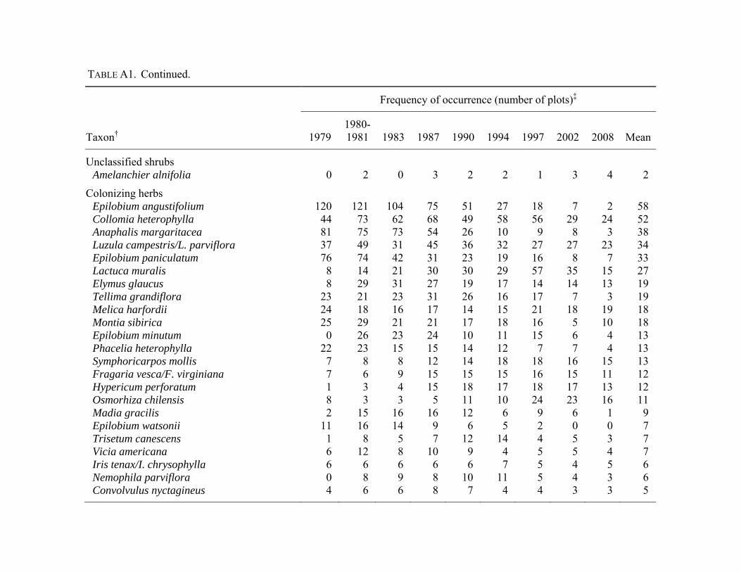
TABLE A1. Continued.
Taxon†
Frequency of occurrence (number of plots)‡
1979 1980- 1981 1983 1987 1990 1994 1997 2002 2008 Mean
Unclassified shrubs Amelanchier alnifolia 0 2 0 3 2 2 1 3 4 2
Colonizing herbs Epilobium angustifolium 120 121 104 75 51 27 18 7 2 58 Collomia heterophylla 44 73 62 68 49 58 56 29 24 52 Anaphalis margaritacea 81 75 73 54 26 10 9 8 3 38 Luzula campestris/L. parviflora 37 49 31 45 36 32 27 27 23 34 Epilobium paniculatum 76 74 42 31 23 19 16 8 7 33 Lactuca muralis 8 14 21 30 30 29 57 35 15 27 Elymus glaucus 8 29 31 27 19 17 14 14 13 19 Tellima grandiflora 23 21 23 31 26 16 17 7 3 19 Melica harfordii 24 18 16 17 14 15 21 18 19 18 Montia sibirica 25 29 21 21 17 18 16 5 10 18 Epilobium minutum 0 26 23 24 10 11 15 6 4 13 Phacelia heterophylla 22 23 15 15 14 12 7 7 4 13 Symphoricarpos mollis 7 8 8 12 14 18 18 16 15 13 Fragaria vesca/F. virginiana 7 6 9 15 15 15 16 15 11 12 Hypericum perforatum 1 3 4 15 18 17 18 17 13 12 Osmorhiza chilensis 8 3 3 5 11 10 24 23 16 11 Madia gracilis 2 15 16 16 12 6 9 6 1 9 Epilobium watsonii 11 16 14 9 6 5 2 0 0 7 Trisetum canescens 1 8 5 7 12 14 4 5 3 7 Vicia americana 6 12 8 10 9 4 5 5 4 7 Iris tenax/I. chrysophylla 6 6 6 6 6 7 5 4 5 6 Nemophila parviflora 0 8 9 8 10 11 5 4 3 6 Convolvulus nyctagineus 4 6 6 8 7 4 4 3 3 5

TABLE A1. Continued.
Taxon†
Frequency of occurrence (number of plots)‡
1979 1980- 1981 1983 1987 1990 1994 1997 2002 2008 Mean
Colonizing herbs (continued) Festuca myuros 4 6 8 11 4 5 2 2 0 5 Gnaphalium microcephalum 7 12 4 7 9 3 2 2 0 5 Lathyrus polyphyllus 5 7 5 6 6 5 6 2 2 5 Montia parvifolia 2 6 3 5 6 6 7 4 4 5 Valeriana scouleri 1 3 4 7 7 6 5 5 3 5 Agoseris grandiflora/A. heterophylla/A. elata 2 5 3 5 3 4 7 4 0 4 Dicentra formosa 5 7 5 3 6 3 3 4 1 4 Aralia californica 5 5 5 4 3 2 2 1 1 3 Boykinia elata 1 1 6 5 6 4 3 2 2 3 Cirsium arvense/C. brevistylum/C. vulgare 3 8 4 0 4 1 2 1 0 3 Lotus micranthus 0 3 4 3 4 3 3 6 2 3 Mitella ovalis 2 0 2 1 2 2 3 7 4 3 Aira caryophyllea 1 3 3 2 2 1 1 0 1 2 Aruncus sylvester 2 1 3 2 2 2 2 1 1 2 Cardamine oligosperma 0 4 3 2 6 4 0 0 0 2 Carex rossii 1 3 1 0 1 2 1 1 7 2 Cynosurus echinatus 0 0 0 4 4 5 2 3 1 2 Deschampsia elongata 1 1 2 2 2 2 3 2 1 2 Gilia capitata 0 2 2 3 1 3 2 1 0 2 Heuchera micrantha 1 2 1 3 2 1 1 1 1 2 Holcus lanatus/H. mollis 1 4 6 3 1 0 0 0 0 2 Lonicera ciliosa 0 0 1 2 2 2 3 3 3 2 Lotus crassifolius 5 2 2 3 3 1 0 1 0 2 Ranunculus uncinatus 0 2 1 3 4 1 1 1 0 2 Agrostis exarata 3 1 1 2 1 1 0 0 0 1
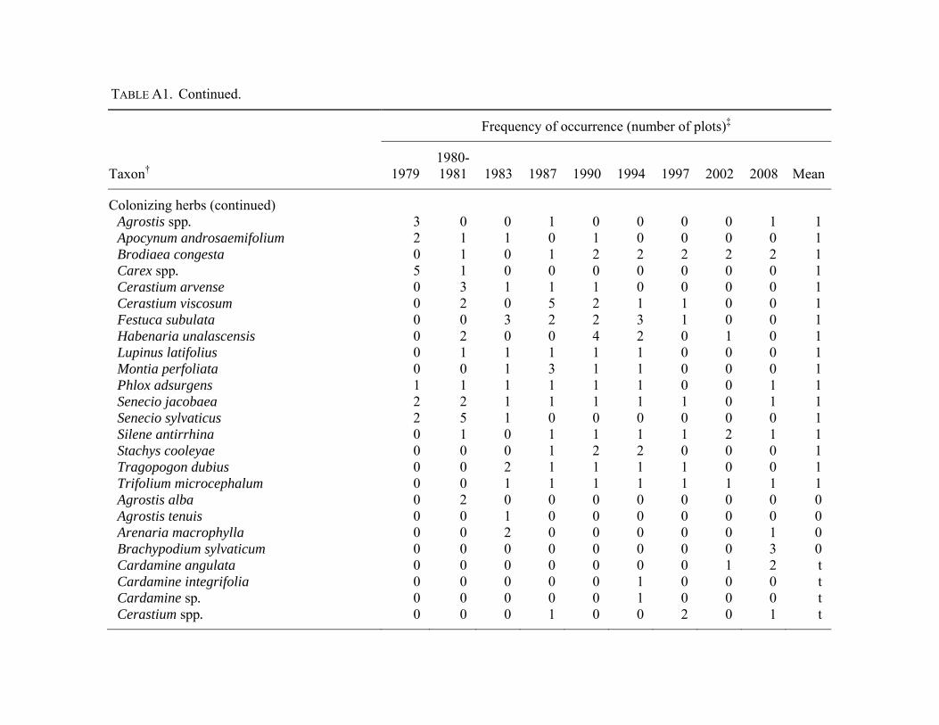
TABLE A1. Continued.
Taxon†
Frequency of occurrence (number of plots)‡
1979 1980- 1981 1983 1987 1990 1994 1997 2002 2008 Mean
Colonizing herbs (continued) Agrostis spp. 3 0 0 1 0 0 0 0 1 1 Apocynum androsaemifolium 2 1 1 0 1 0 0 0 0 1 Brodiaea congesta 0 1 0 1 2 2 2 2 2 1 Carex spp. 5 1 0 0 0 0 0 0 0 1 Cerastium arvense 0 3 1 1 1 0 0 0 0 1 Cerastium viscosum 0 2 0 5 2 1 1 0 0 1 Festuca subulata 0 0 3 2 2 3 1 0 0 1 Habenaria unalascensis 0 2 0 0 4 2 0 1 0 1 Lupinus latifolius 0 1 1 1 1 1 0 0 0 1 Montia perfoliata 0 0 1 3 1 1 0 0 0 1 Phlox adsurgens 1 1 1 1 1 1 0 0 1 1 Senecio jacobaea 2 2 1 1 1 1 1 0 1 1 Senecio sylvaticus 2 5 1 0 0 0 0 0 0 1 Silene antirrhina 0 1 0 1 1 1 1 2 1 1 Stachys cooleyae 0 0 0 1 2 2 0 0 0 1 Tragopogon dubius 0 0 2 1 1 1 1 0 0 1 Trifolium microcephalum 0 0 1 1 1 1 1 1 1 1 Agrostis alba 0 2 0 0 0 0 0 0 0 0 Agrostis tenuis 0 0 1 0 0 0 0 0 0 0 Arenaria macrophylla 0 0 2 0 0 0 0 0 1 0 Brachypodium sylvaticum 0 0 0 0 0 0 0 0 3 0 Cardamine angulata 0 0 0 0 0 0 0 1 2 t Cardamine integrifolia 0 0 0 0 0 1 0 0 0 t Cardamine sp. 0 0 0 0 0 1 0 0 0 t Cerastium spp. 0 0 0 1 0 0 2 0 1 t

TABLE A1. Continued.
Taxon†
Frequency of occurrence (number of plots)‡
1979 1980- 1981 1983 1987 1990 1994 1997 2002 2008 Mean
Colonizing herbs (continued) Cerastium vulgatum 1 0 2 1 0 0 0 0 0 t Chrysanthemum leucanthemum 0 1 1 1 0 0 0 0 0 t Conyza canadensis 0 2 0 0 0 0 0 0 0 t Cruciferae sp. 0 0 0 0 0 1 0 0 0 t Cystopteris fragilis 0 0 0 0 0 3 0 0 0 t Epilobium spp. 0 0 0 0 0 0 2 0 0 t Erechtites hieracifolia 0 0 0 1 0 0 0 0 0 t Festuca subulifolia 0 0 0 0 0 0 1 1 1 t Gnaphalium purpureum 0 0 0 0 0 0 1 1 0 t Hierochloe occidentalis 1 0 0 0 0 0 0 0 0 t Hypochaeris radicata 2 1 0 0 0 0 0 0 0 t Juncus sp. 1 0 0 0 0 0 0 0 0 t Lepidium campestre 0 0 1 0 0 0 0 0 0 t Lonicera spp. 0 0 0 0 0 1 1 1 0 t Mimulus alsinoides 0 0 1 0 0 1 0 0 0 t Mimulus guttatus 0 1 0 1 0 0 0 0 0 t Pachistima myrsinites 0 1 0 0 0 0 0 0 0 t Polypodiaceae sp. 0 0 0 0 0 1 0 0 0 t Sedum oreganum 0 0 1 0 1 0 0 0 0 t Stellaria crispa 0 0 0 0 0 0 0 1 0 t Stellaria spp. 0 0 0 0 1 1 1 0 0 t
Residual forest herbs Rubus ursinus 165 162 164 166 166 166 164 161 153 163 Berberis nervosa 109 113 111 123 125 130 134 141 148 126 Trientalis latifolia 152 153 138 136 121 117 110 75 68 119

TABLE A1. Continued.
Taxon†
Frequency of occurrence (number of plots)‡
1979 1980- 1981 1983 1987 1990 1994 1997 2002 2008 Mean
Residual forest herbs (continued) Polystichum munitum 87 85 99 119 121 127 134 128 130 114 Gaultheria shallon 52 55 62 69 74 77 76 75 68 67 Whipplea modesta 77 72 78 83 71 65 63 44 42 66 Viola sempervirens 57 61 60 71 67 66 63 60 55 62 Hieracium albiflorum 81 89 65 75 65 51 52 40 26 61 Linnaea borealis 37 36 39 45 40 41 41 42 32 39 Coptis laciniata 32 31 33 42 40 43 40 40 39 38 Chimaphila menziesii 0 2 2 8 21 38 60 60 66 29 Festuca occidentalis 38 36 28 36 30 28 25 21 15 29 Vancouveria hexandra 21 23 28 28 32 31 30 24 25 27 Pteridium aquilinum 20 24 29 34 32 27 26 21 17 26 Trillium ovatum 8 12 9 16 27 34 30 33 42 24 Campanula scouleri 20 23 19 34 30 28 23 16 14 23 Smilacina stellata/S. racemosa 14 16 12 32 27 34 22 23 23 23 Anemone deltoidea 7 7 11 16 20 35 28 22 25 19 Bromus vulgaris 28 17 8 25 22 20 19 19 14 19 Achlys triphylla 11 13 11 15 11 13 12 9 10 12 Liliaceae spp. 0 0 1 1 1 13 20 35 22 10 Adiantum pedatum 5 5 9 11 11 13 11 11 8 9 Oxalis oregana 10 9 9 9 8 7 9 8 8 9 Rubus nivalis 14 12 8 11 14 6 7 7 6 9 Tiarella trifoliata 4 7 4 9 9 8 9 7 6 7 Asarum caudatum 5 4 4 8 10 7 8 6 5 6 Chimaphila umbellata 3 4 2 6 5 8 10 7 8 6 Disporum hookeri/D. smithii 3 5 3 5 6 7 10 9 10 6

TABLE A1. Continued.
Taxon†
Frequency of occurrence (number of plots)‡
1979 1980- 1981 1983 1987 1990 1994 1997 2002 2008 Mean
Residual forest herbs (continued) Galium oreganum 5 4 15 9 6 4 4 4 2 6 Synthyris reniformis 1 4 1 5 6 6 6 11 15 6 Xerophyllum tenax 5 5 6 4 6 7 7 6 7 6 Actaea rubra 2 5 2 8 5 3 2 1 4 4 Athyrium filix-femina 2 3 2 2 3 3 6 3 3 3 Petasites frigidus 0 3 4 3 4 3 4 3 2 3 Anemone lyallii 3 3 0 0 2 2 2 3 4 2 Arnica discoidea 0 1 0 3 2 3 3 3 2 2 Goodyera oblongifolia 2 2 1 2 1 2 3 4 5 2 Polypodium glycyrrhiza 1 2 1 2 2 3 3 0 0 2 Pyrola asarifolia 1 2 1 3 4 1 3 3 1 2 Adenocaulon bicolor 3 2 1 0 0 1 1 1 0 1 Blechnum spicant 0 0 0 0 1 1 1 2 3 1 Lilium columbianum 0 0 0 0 0 1 2 2 1 1 Pyrola picta 0 0 0 0 1 1 1 2 2 1 Trisetum cernuum 0 0 0 0 1 1 1 1 1 1 Circaea alpina 0 0 0 0 0 0 2 0 0 t Clintonia uniflora 0 0 1 0 1 1 1 0 0 t Listera caurina 0 1 0 0 0 0 1 1 1 t Listera cordata 0 0 0 0 0 1 0 1 0 t Listera sp. 0 0 0 0 1 0 0 0 0 t Saxifragaceae sp. 0 0 0 0 0 0 0 0 1 t
Unclassified herbs Galium triflorum/G. aparine 93 128 121 124 117 118 120 80 72 108 Poaceae spp. 14 0 5 19 18 10 22 2 7 11 Equisetum telmateia 2 2 2 3 2 1 1 1 0 2

TABLE A1. Continued.
Taxon†
Frequency of occurrence (number of plots)‡
1979 1980- 1981 1983 1987 1990 1994 1997 2002 2008 Mean
Unclassified herbs (continued) Festuca spp. 1 0 1 0 0 0 0 0 1 t Tolmiea menziesii 0 0 0 1 1 1 0 0 1 t
†Shrubs include woody taxa ≥1m tall at maturity; herbs include low shrubs (<1 m) and subshrubs. ‡Total number of plots = 188. t = trace (<1).

TABLE A2. Mean cover of understory taxa in WS1 and WS3, H. J. Andrews Experimental Forest, Oregon, over the study period (1979-2008). Within each group, taxa are arranged in descending order of mean cover over the study period (Mean). Nomenclature follows Hitchcock and Cronquist (1973).
Taxon†
Cover (%)
1979 1980- 1981 1983 1987 1990 1994 1997 2002 2008 Mean
Colonizing shrubs Ceanothus sanguineus 10.86 13.15 15.37 9.48 7.47 2.12 1.81 0.71 0.13 6.79Ceanothus velutinus 13.49 12.48 12.99 0.46 0.14 t 0 0 0 4.40Salix scouleriana 1.63 1.64 2.51 2.34 1.37 1.02 0.91 0.08 0 1.28Ceanothus integerrimus 1.52 1.64 2.23 1.59 1.39 0.81 1.09 0.23 0.10 1.18Oemleria cerasiformis 0.43 0.52 0.53 0.51 0.46 0.64 0.65 0.69 0.52 0.55Sambucus cerulea 0.20 0.34 0.91 0.73 0.21 0.27 0.47 0.32 0.03 0.39Arctostaphylos columbiana 0.80 0.76 0.81 0.10 0.11 0.13 0.21 0.16 0.37 0.38Ribes sanguineum/R. lobbii/R. lacustre 0.27 0.34 0.25 0.29 0.23 0.07 0.05 t t 0.17Rubus leucodermis 0.44 0.18 0.14 0.11 0.05 0.02 0.03 0.04 0.02 0.11Salix sitchensis 0.03 0.07 0.04 0.14 0.18 t 0.08 0.07 0.03 0.07Acer glabrum 0 t t 0.01 t t 0.01 0.01 0.01 t
Residual forest shrubs Acer circinatum 9.16 10.23 13.03 16.68 20.82 21.80 30.39 31.36 27.13 20.07Rhododendron macrophyllum 3.58 4.01 5.95 6.00 5.71 5.16 5.67 4.53 3.51 4.90Rubus parviflorus 8.73 9.75 10.22 7.04 4.73 1.73 0.84 0.42 0.12 4.84Corylus conuta 1.72 1.90 2.80 2.65 2.81 2.39 2.59 2.41 2.38 2.41Vaccinium parvifolium 0.93 0.88 1.56 1.55 1.40 1.52 2.27 2.04 1.07 1.47Holodiscus discolor 0.28 0.32 0.55 0.54 0.58 0.57 1.03 1.10 1.26 0.69Rosa gymnocarpa 0.95 1.00 1.09 0.85 0.36 0.19 0.44 0.20 0.19 0.58Rhus diversiloba 0.08 0.14 0.12 0.17 0.12 0.19 0.54 0.27 0.48 0.23Vaccinium membranaceum 0.12 0.17 0.11 0.29 0.16 0.13 0.10 0.06 t 0.13Alnus sinuata 0.02 0.01 0.08 0.04 0.09 0.27 0.16 0.11 0.05 0.09

TABLE A2. Continued.
Taxon†
Cover (%)
1979 1980- 1981 1983 1987 1990 1994 1997 2002 2008 Mean
Unclassified shrubs Amelanchier alnifolia 0 0.03 0 0.08 0.04 t 0.06 0.29 0.11 0.07
Colonizing herbs Epilobium angustifolium 5.23 3.82 2.64 1.22 0.60 0.09 0.05 0.01 t 1.52Symphoricarpos mollis 0.73 0.76 0.68 0.61 0.61 0.73 0.71 0.34 0.36 0.62Melica harfordii 1.95 1.32 1.03 0.38 0.15 0.06 0.11 0.06 0.06 0.57Anaphalis margaritacea 2.24 1.19 0.82 0.26 0.11 0.02 t 0.01 t 0.52Epilobium paniculatum 1.96 1.58 0.21 0.08 0.05 0.02 0.02 0.01 t 0.44Aralia californica 0.24 0.20 0.27 0.77 0.70 0.59 0.44 0.02 0.05 0.36Elymus glaucus 0.67 1.21 0.63 0.15 0.08 0.04 0.11 0.04 0.04 0.33Festuca myuros 0.40 0.52 0.81 0.49 0.01 0.03 0.01 t 0 0.25Lactuca muralis 0.15 0.18 0.15 0.19 0.31 0.28 0.41 0.12 0.09 0.21Boykinia elata 0.21 0.27 0.39 0.25 0.19 0.06 0.11 0.23 0.06 0.20Collomia heterophylla 0.62 0.69 0.16 0.13 0.04 0.04 0.05 0.03 0.03 0.20Heuchera micrantha 0.11 0.18 0.10 0.18 0.20 0.21 0.25 0.24 0.07 0.17Montia sibirica 0.15 0.66 0.25 0.08 0.07 0.04 0.03 0.04 0.19 0.17Convolvulus nyctagineus 0.18 0.57 0.39 0.08 0.08 0.04 0.07 t t 0.16Luzula campestris/L. parviflora 0.33 0.41 0.23 0.14 0.05 0.03 0.04 0.05 0.04 0.15Tellima grandiflora 0.20 0.33 0.14 0.20 0.12 0.13 0.05 0.05 t 0.14Vicia americana 0.13 0.39 0.19 0.07 0.03 0.11 0.09 0.06 0.03 0.12Fragaria vesca/F. virginiana 0.16 0.14 0.09 0.16 0.16 0.06 0.12 0.07 0.06 0.11Madia gracilis t 0.16 0.14 0.22 0.36 t 0.03 t t 0.10Hypericum perforatum t t 0.01 0.08 0.17 0.07 0.24 0.15 0.11 0.09Phacelia heterophylla 0.18 0.24 0.09 0.07 0.09 0.02 0.05 0.02 0.01 0.09Cynosurus echinatus 0 0 0 0.03 0.15 0.27 0.26 0.01 t 0.08Lathyrus polyphyllus 0.09 0.14 0.16 0.11 0.04 0.02 0.05 t t 0.07

TABLE A2. Continued.
Taxon†
Cover (%)
1979 1980- 1981 1983 1987 1990 1994 1997 2002 2008 Mean
Colonizing herbs (continued) Valeriana scouleri 0.02 0.04 0.05 0.09 0.11 0.06 0.10 0.12 0.01 0.07Lotus crassifolius 0.23 0.13 0.14 0.04 0.02 t 0 0.01 0 0.06Epilobium minutum 0 0.38 0.03 0.04 t 0.01 0.01 t t 0.05Montia parvifolia 0.02 0.12 0.02 t 0.02 0.02 0.19 0.01 0.01 0.05Osmorhiza chilensis 0.08 0.04 0.05 0.02 0.02 0.02 0.07 0.07 0.05 0.05Iris tenx/I. chrysophylla 0.09 0.07 0.05 0.02 0.01 t 0.03 0.03 0.02 0.04Aruncus sylvester 0.02 0.05 0.09 0.03 0.08 0.01 t t t 0.03Dicentra formosa 0.04 0.03 0.01 0.03 0.05 0.06 0.01 t t 0.03Epilobium watsonii 0.10 0.10 0.06 0.01 t 0.02 t 0 0 0.03Phlox adsurgens 0.08 0.09 0.05 0.02 t t 0 0 t 0.03Trisetum canescens t 0.08 0.03 0.02 0.04 0.03 t 0.01 0.02 0.03Aira caryophyllea t 0.09 0.02 0.06 t t t 0 t 0.02Apocynum androsaemifolium 0.13 t 0.03 0 t 0 0 0 0 0.02Gilia capitata 0 0.05 0.05 0.03 0.02 t t t 0 0.02Gnaphalium microcephalum 0.01 0.05 0.03 0.01 0.03 0.01 t t 0 0.02Holcus lanatus/H. mollis 0.01 0.05 0.11 t t 0 0 0 0 0.02Lonicera ciliosa 0 0 t 0.06 0.03 t 0.02 0.01 t 0.02Lotus micranthus 0 0.08 0.03 t t 0.03 t t t 0.02Nemophila parviflora 0 0.09 0.04 0.02 t t t t t 0.02Agoseris grandiflora/A. heterophylla/A. elata t 0.03 t 0.01 0.01 0.01 0.01 t 0 0.01Brodiaea congesta 0 t 0 t t 0.04 0.02 t 0.02 0.01Carex rossii t 0.02 0.01 0 0.03 0.02 0.01 t 0.01 0.01Deschampsia elongata 0.02 0.05 t 0.01 t t 0.03 t t 0.01Agrostis alba 0 t 0 0 0 0 0 0 0 tAgrostis exarata 0.02 0.01 0.01 t t t 0 0 0 t

TABLE A2. Continued.
Taxon†
Cover (%)
1979 1980- 1981 1983 1987 1990 1994 1997 2002 2008 Mean
Colonizing herbs (continued) Agrostis spp. 0.04 0 0 t 0 0 0 0 t tAgrostis tenuis 0 0 t 0 0 0 0 0 0 tArenaria macrophylla 0 0 t 0 0 0 0 0 t tBrachypodium sylvaticum 0 0 0 0 0 0 0 0 0.03 tCardamine angulata 0 0 0 0 0 0 0 t t tCardamine integrifolia 0 0 0 0 0 t 0 0 0 tCardamine oligosperma 0 t t t t t 0 0 0 tCardamine spp. 0 0 0 0 0 t 0 0 0 tCarex spp. 0.03 t 0 0 0 0 0 0 0 tCerastium arvense 0 0.03 t t t 0 0 0 0 tCerastium spp. 0 0 0 t 0 0 t 0 t tCerastium viscosum 0 0.03 0 0.01 0.01 t t 0 0 tCerastium vulgatum t 0 0.01 0.02 0 0 0 0 0 tChrysanthemum leucanthemum 0 t t t 0 0 0 0 0 tCirsium arvense/C. brevistylum/C. vulgare 0.04 0.04 t 0 t t t t 0 tConyza canadensis 0 t 0 0 0 0 0 0 0 tCruciferae sp. 0 0 0 0 0 t 0 0 0 tCystopteris fragilis 0 0 0 0 0 t 0 0 0 tEpilobium spp. 0 0 0 0 0 0 t 0 0 tErechtites hieracifolia 0 0 0 t 0 0 0 0 0 tFestuca subulata 0 0 0.01 t t t t 0 0 tFestuca subulifolia 0 0 0 0 0 0 t t t tGnaphalium purpureum 0 0 0 0 0 0 t t 0 tHabenaria unalascensis 0 0.02 0 0 t t 0 t 0 tHierochloe occidentalis t 0 0 0 0 0 0 0 0 t

TABLE A2. Continued.
Taxon†
Cover (%)
1979 1980- 1981 1983 1987 1990 1994 1997 2002 2008 Mean
Colonizing herbs (continued) Hypochaeris radicata t t 0 0 0 0 0 0 0 tJuncus sp. t 0 0 0 0 0 0 0 0 tLepidium campestre 0 0 t 0 0 0 0 0 0 tLonicera spp. 0 0 0 0 0 t t t 0 tLupinus latifolius 0 t 0.02 t 0.01 t 0 0 0 tMimulus alsinoides 0 0 t 0 0 t 0 0 0 tMimulus guttatus 0 t 0 t 0 0 0 0 0 tMitella ovalis t 0 t t t t t t 0.06 tMontia perfoliata 0 0 t t t t 0 0 0 tPachistima myrsinites 0 t 0 0 0 0 0 0 0 tPolypodiaceae sp. 0 0 0 0 0 t 0 0 0 tRanunculus uncinatus 0 0.01 0.03 t t t t t 0 tSedum oreganum 0 0 t 0 t 0 0 0 0 tSenecio jacobaea 0.03 0.02 t t t t t 0 t tSenecio sylvaticus t t t 0 0 0 0 0 0 tSilene antirrhina 0 0.02 0 t t t t t t tStachys cooleyae 0 0 0 t t t 0 0 0 tStellaria crispa 0 0 0 0 0 0 0 t 0 tStellaria spp. 0 0 0 0 t t t 0 0 tTragopogon dubius 0 0 t t t t t 0 0 tTrifolium microcephalum 0 0 t t t t t t t t
Residual forest herbs Rubus ursinus 20.46 18.58 16.70 14.18 8.80 3.16 5.83 2.79 1.89 10.27Berberis nervosa 5.03 4.82 4.87 7.64 8.33 9.77 15.69 14.47 14.95 9.51Polystichum munitum 3.80 4.83 6.06 9.59 10.68 9.93 13.48 11.88 13.16 9.27

TABLE A2. Continued.
Taxon†
Cover (%)
1979 1980- 1981 1983 1987 1990 1994 1997 2002 2008 Mean
Residual forest herbs (continued) Gaultheria shallon 6.29 5.33 6.40 7.94 8.09 6.20 9.45 6.70 4.81 6.80Whipplea modesta 3.83 2.32 1.86 1.67 1.38 0.74 1.09 0.71 0.64 1.58Trientalis latifolia 4.47 3.41 1.38 1.43 0.97 0.36 0.64 0.42 0.29 1.48Linnaea borealis 2.06 2.13 1.89 1.54 1.05 1.03 0.78 0.85 0.36 1.30Vancouveria hexandra 1.45 1.85 1.43 1.07 0.51 0.34 0.48 0.45 0.19 0.86Oxalis oregana 1.21 0.91 1.15 0.84 0.69 0.43 0.47 0.21 0.19 0.68Viola sempervirens 0.47 0.55 0.41 0.48 0.39 0.22 0.29 0.25 0.56 0.40Coptis laciniata 0.68 0.72 0.42 0.25 0.19 0.16 0.22 0.25 0.29 0.35Smilacina stellata/S. racemosa 0.30 0.40 0.18 0.30 0.15 0.12 0.36 0.16 0.07 0.23Petasites frigidus 0 0.15 0.13 0.40 0.35 0.27 0.20 0.08 t 0.18Hieracium albiflorum 0.26 0.37 0.19 0.18 0.15 0.08 0.11 0.13 0.06 0.17Festuca occidentalis 0.55 0.40 0.17 0.10 0.05 0.08 0.04 0.02 0.04 0.16Xerophyllum tenax 0.16 0.17 0.11 0.09 0.13 0.16 0.22 0.17 0.17 0.15Adiantum pedatum 0.07 0.07 0.08 0.22 0.21 0.10 0.28 0.10 0.09 0.14Bromus vulgaris 0.43 0.14 0.02 0.16 0.09 0.07 0.14 0.13 0.08 0.14Achlys triphylla 0.26 0.26 0.19 0.18 0.08 0.05 0.06 0.03 0.02 0.13Athyrium filix-femina 0.08 0.14 0.05 0.11 0.14 0.23 0.15 0.04 0.06 0.11Galium oreganum 0.24 0.19 0.17 0.05 0.03 t t t t 0.08Campanula scouleri 0.10 0.10 0.05 0.13 0.08 0.04 0.06 0.05 0.04 0.07Trillium ovatum 0.03 0.07 0.04 0.07 0.10 0.06 0.07 0.08 0.08 0.07Chimaphila menziesii 0 t t t 0.02 0.04 0.12 0.16 0.10 0.05Anemone deltoidea 0.04 0.05 0.04 0.06 0.05 0.03 0.03 0.04 0.05 0.04Tiarella trifoliata 0.05 0.06 0.05 0.05 0.03 0.01 0.05 0.02 0.02 0.04Asarum caudatum 0.03 0.03 0.02 0.04 0.02 0.03 0.05 0.06 0.02 0.03Disporum hookeri/D. smithii 0.02 0.03 0.01 0.03 0.01 0.01 0.05 0.04 0.05 0.03

TABLE A2. Continued.
Taxon†
Cover (%)
1979 1980- 1981 1983 1987 1990 1994 1997 2002 2008 Mean
Residual forest herbs (continued) Rubus nivalis 0.06 0.05 0.03 0.05 0.03 0.01 0.04 0.01 t 0.03Actaea rubra 0.02 0.04 0.02 0.04 0.02 t t t t 0.02Synthyris reniformis 0.02 0.02 t 0.01 0.01 0.01 0.01 0.02 0.03 0.02Adenocaulon bicolor 0.06 0.03 0.03 0 0 t t t 0 0.01Chimaphila umbellata 0.02 0.02 0.01 0.02 0.01 0.01 0.01 t 0.01 0.01Pyrola asarifolia 0.01 0.03 t 0.02 0.01 t t t t 0.01Anemone lyallii t 0.04 0 0 t t t t t tArnica discoidea 0 t 0 t t t t t t tBlechnum spicant 0 0 0 0 t t t t 0.03 tCircaea alpina 0 0 0 0 0 0 t 0 0 tClintonia uniflora 0 0 t 0 t t t 0 0 tGoodyera oblongifolia 0.01 t t t t t t t t tLiliaceae spp. 0 0 t t t t 0.01 0.02 0.01 tLilium columbianum 0 0 0 0 0 t t t t tListera caurina 0 t 0 0 0 0 t t t tListera cordata 0 0 0 0 0 t 0 t 0 tListera sp. 0 0 0 0 t 0 0 0 0 tPolypodium glycyrrhiza t t t t t t t 0 0 tPyrola picta 0 0 0 0 t t t t t tSaxifragaceae sp. 0 0 0 0 0 0 0 0 t tTrisetum cernuum 0 0 0 0 t t 0.02 0.02 0.01 t
Unclassified herbs Galium triflorum/G. aparine 1.11 1.85 1.38 0.67 0.42 0.28 0.29 0.23 0.18 0.71Equisetum telmateia 0.03 0.05 0.13 0.08 t 0.02 t t 0 0.04Poaceae spp. 0.15 0 t 0.02 0.01 0.01 0.03 t t 0.03

TABLE A2. Continued.
†Shrubs include woody taxa ≥1m tall at maturity; herbs include low shrubs (<1 m) and subshrubs. t = trace (<0.01%).
Taxon†
Cover (%)
1979 1980- 1981 1983 1987 1990 1994 1997 2002 2008 Mean
Unclassified herbs (continued) Festuca spp. 0.04 0 t 0 0 0 0 0 t tTolmiea menziesii 0 0 0 t t t 0 0 t t

TABLE A3. Mean biomass of understory taxa in WS1 and WS3, H. J. Andrews Experimental Forest, Oregon, over the study period (1979-2008). Within each group, taxa are arranged in descending order of mean biomass over the study period (Mean). Nomenclature follows Hitchcock and Cronquist (1973).
Taxon†
Biomass (Mg/ha)
1979 1980- 1981 1983 1987 1990 1994 1997 2002 2008 Mean
Colonizing shrubs Ceanothus sanguineus 2.244 2.342 2.364 1.661 0.743 0.249 0.263 0.010 0.002 1.098 Ceanothus velutinus 2.570 2.263 2.040 0.056 0.042 t 0 0 0 0.775 Salix scouleriana 0.248 0.361 0.298 0.642 0.628 0.954 0.882 t 0 0.446 Ceanothus integerrimus 0.189 0.151 0.096 0.149 0.165 0.049 0.050 0.001 t 0.095 Arctostaphylos columbiana 0.143 0.236 0.188 0.149 0 0.021 0.066 0 0 0.089 Oemleria cerasiformis 0.032 0.030 0.027 0.061 0.044 0.064 0.023 0.004 0 0.032 Ribes sanguineum/R. lobbii/R. lacustre 0.050 0.051 0.022 0.009 0.005 0.004 0.005 0.001 0.002 0.017 Salix sitchensis t 0.001 0.004 0.032 0.031 0.002 0.083 0 0 0.017 Acer glabrum 0 0 t t t t t t t t Rubus leucodermis 0 0 0.004 t t t t t t t Sambucus cerulea t 0.006 0 0 0 t 0 0 0 t
Residual forest shrubs Acer circinatum 2.322 2.673 2.816 3.802 4.071 5.954 5.557 6.184 5.595 4.330 Rhododendron macrophyllum 0.642 0.764 0.936 1.369 1.227 1.002 0.873 0.594 0.446 0.873 Corylus conuta 0.430 0.600 0.459 0.648 0.613 1.010 0.472 0.264 0.209 0.523 Vaccinium parvifolium 0.102 0.127 0.126 0.160 0.159 0.134 0.212 0.101 0.094 0.135 Rubus parviflorus 0.177 0.198 0.207 0.143 0.096 0.035 0.017 0.009 0.002 0.098 Holodiscus discolor 0.012 0.016 0.021 0.034 0.056 0.034 0.044 0.042 0.117 0.042 Alnus sinuata t t 0.004 0.033 0.062 0.086 0.110 0.002 0.046 0.038 Rosa gymnocarpa 0.050 0.079 0.047 0.022 0.020 0.006 0.007 0.006 0.002 0.026 Vaccinium membranaceum 0.007 0.006 0.006 0.019 0.011 0.015 0.007 0.005 t 0.008 Rhus diversiloba 0.006 0.003 0.003 0.004 0.002 0.001 0.006 0.002 0.014 0.005

TABLE A3. Continued.
Taxon†
Biomass (Mg/ha)
1979 1980- 1981 1983 1987 1990 1994 1997 2002 2008 Mean
Unclassified shrubs Amelanchier alnifolia 0 0 0 t t t 0 t t t
Colonizing herbs Epilobium angustifolium 0.252 0.185 0.127 0.059 0.029 0.004 0.003 t t 0.073 Epilobium paniculatum 0.083 0.066 0.009 0.003 0.002 t t t t 0.018 Luzula campestris/L. parviflora 0.026 0.049 0.015 0.004 t t t t t 0.011 Melica harfordii 0.038 0.025 0.020 0.007 0.003 0.001 0.002 0.001 0.001 0.011 Symphoricarpos mollis 0.013 0.014 0.012 0.011 0.011 0.013 0.013 0.006 0.007 0.011 Elymus glaucus 0.010 0.019 0.011 0.004 0.003 0.002 0.003 0.002 0.001 0.006 Aralia californica 0 0.002 0.003 0.007 0.014 0.008 0.001 0.004 t 0.005 Anaphalis margaritacea 0.019 0.010 0.007 0.002 t t t t t 0.004 Lactuca muralis 0.003 0.004 0.004 0.005 0.006 0.005 0.007 0.003 0.002 0.004 Tellima grandiflora 0.004 0.004 0.003 0.005 0.004 0.003 0.002 0.001 t 0.003 Collomia heterophylla 0.007 0.008 0.002 t t t t t t 0.002 Convolvulus nyctagineus 0.002 0.009 0.005 t t t t t t 0.002 Cynosurus echinatus 0 0 0 t 0.003 0.005 0.005 t t 0.002 Epilobium minutum 0 0.016 0.001 0.002 t t t t t 0.002 Montia sibirica 0.002 0.008 0.003 t t t t t t 0.002 Boykinia elata 0.001 0.001 0.003 0.002 0.002 t t 0.001 t 0.001 Festuca myuros 0.002 0.003 0.004 0.003 t t t t 0 0.001 Heuchera micrantha t 0.001 t 0.001 0.001 0.001 0.001 0.001 t 0.001 Hypericum perforatum t t t t 0.002 t 0.003 0.002 0.001 0.001 Lotus crassifolius 0.004 0.002 0.002 t t t 0 t 0 0.001 Madia gracilis 0 0.002 0.002 0.002 0.003 t t t 0 0.001 Phacelia heterophylla 0.002 0.003 0.001 t 0.001 t t t t 0.001 Agoseris grandiflora/A. heterophylla/A. elata t t t t t t t t 0 t

TABLE A3. Continued.
Taxon†
Biomass (Mg/ha)
1979 1980- 1981 1983 1987 1990 1994 1997 2002 2008 Mean
Colonizing herbs (continued) Agrostis alba 0 t 0 0 0 0 0 0 0 t Agrostis exarata t t t t t t 0 0 0 t Agrostis spp. t 0 0 t 0 0 0 0 t t Agrostis tenuis 0 0 t 0 0 0 0 0 0 t Aira caryophyllea t t t t t t t 0 t t Apocynum androsaemifolium 0.002 t t 0 t 0 0 0 0 t Arenaria macrophylla 0 0 t 0 0 0 0 0 t t Aruncus sylvester t 0.001 0.002 t 0.002 t t t t t Brachypodium sylvaticum 0 0 0 0 0 0 0 0 t t Brodiaea congesta 0 t 0 t t t t t t t Cardamine angulata 0 0 0 0 0 0 0 t t t Cardamine integrifolia 0 0 0 0 0 t 0 0 0 t Cardamine oligosperma 0 t t t t t 0 0 0 t Cardamine spp. t t 0 0 0 0 0 0 0 t Carex rossii t t t 0 t t t t t t Carex spp. t t 0 0 0 0 0 0 0 t Cerastium arvense 0 t t t t 0 0 0 0 t Cerastium spp. 0 0 0 t 0 0 t 0 t t Cerastium viscosum 0 t 0 t t t t 0 0 t Cerastium vulgatum t 0 t t 0 0 0 0 0 t Chrysanthemum leucanthemum 0 t t t 0 0 0 0 0 t Cirsium arvense/C. brevistylum/C. vulgare t t t 0 t t t t 0 t Conyza canadensis 0 t 0 0 0 0 0 0 0 t Cruciferae sp. 0 0 0 0 0 t 0 0 0 t Cystopteris fragilis 0 0 0 0 0 t 0 0 0 t

TABLE A3. Continued.
Taxon†
Biomass (Mg/ha)
1979 1980- 1981 1983 1987 1990 1994 1997 2002 2008 Mean
Colonizing herbs (continued) Deschampsia elongata t t t t t t t t t t Dicentra formosa t t t t t t t t t t Epilobium spp. 0 0 0 0 0 0 t 0 0 t Epilobium watsonii 0.002 0.002 t t t t t 0 0 t Erechtites hieracifolia 0 0 0 t 0 0 0 0 0 t Festuca subulata 0 0 t t t t t 0 0 t Festuca subulifolia 0 0 0 0 0 0 t t t t Fragaria vesca/F. virginiana 0.001 0.001 t 0.001 0.001 t 0.001 t t t Gilia capitata 0 t t t t t t t 0 t Gnaphalium microcephalum t 0.001 t t t t t t 0 t Gnaphalium purpureum 0 0 0 0 0 0 t t 0 t Habenaria unalascensis 0 t 0 0 t t 0 t 0 t Hierochloe occidentalis t 0 0 0 0 0 0 0 0 t Holcus lanatus/H. mollis t t 0.002 t t 0 0 0 0 t Hypochaeris radicata t t 0 0 0 0 0 0 0 t Iris tenx/I. chrysophylla 0.002 0.001 t t t t t t t t Juncus sp. t 0 0 0 0 0 0 0 0 t Lathyrus polyphyllus t t 0.001 t t t t t t t Lepidium campestre 0 0 t 0 0 0 0 0 0 t Lonicera ciliosa 0 0 t t t t t t t t Lonicera spp. 0 0 0 0 0 t t t 0 t Lotus micranthus 0 0.001 t t t t t t t t Lupinus latifolius 0 t t t t t 0 0 0 t Mimulus alsinoides 0 0 t 0 0 t 0 0 0 t Mimulus guttatus 0 t 0 t 0 0 0 0 0 t

TABLE A3. Continued.
Taxon†
Biomass (Mg/ha)
1979 1980- 1981 1983 1987 1990 1994 1997 2002 2008 Mean
Colonizing herbs (continued) Mitella ovalis t 0 t t t t t t t t Montia parvifolia t 0.001 t t t t 0.002 t t t Montia perfoliata 0 0 t t t t 0 0 0 t Nemophila parviflora 0 0.001 t t t t t t t t Osmorhiza chilensis t t t t t t t t t t Pachistima myrsinites 0 t 0 0 0 0 0 0 0 t Phlox adsurgens 0.001 0.001 t t t t 0 0 t t Polypodiaceae sp. 0 0 0 0 0 t 0 0 0 t Ranunculus uncinatus 0 t t t t t t t 0 t Sedum oreganum 0 0 t 0 t 0 0 0 0 t Senecio jacobaea t t t t t t t 0 t t Senecio sylvaticus t t t 0 0 0 0 0 0 t Silene antirrhina 0 t 0 t t t t t t t Stachys cooleyae 0 0 0 t t t 0 0 0 t Stellaria crispa 0 0 0 0 0 0 0 t 0 t Stellaria spp. 0 0 0 0 t t t 0 0 t Tragopogon dubius 0 0 t t t t t 0 0 t Trifolium microcephalum 0 0 t t t t t t t t Trisetum canescens t 0.002 t t t t t t t t Valeriana scouleri t t t 0.001 0.001 0.001 0.001 0.001 t t Vicia americana t 0.002 0.001 t t t t t t t
Residual forest herbs Berberis nervosa 0.307 0.296 0.304 0.501 0.546 0.664 1.127 1.035 1.069 0.650 Gaultheria shallon 0.333 0.290 0.345 0.422 0.433 0.347 0.498 0.369 0.276 0.368 Polystichum munitum 0.076 0.096 0.120 0.189 0.210 0.195 0.264 0.233 0.258 0.182

TABLE A3. Continued.
Taxon†
Biomass (Mg/ha)
1979 1980- 1981 1983 1987 1990 1994 1997 2002 2008 Mean
Residual forest herbs (continued) Rubus ursinus 0.331 0.298 0.264 0.210 0.111 0.029 0.067 0.025 0.016 0.150 Whipplea modesta 0.139 0.082 0.065 0.058 0.048 0.025 0.038 0.024 0.022 0.056 Pteridium aquilinum 0.016 0.044 0.050 0.073 0.056 0.038 0.015 0.004 0.004 0.033 Xerophyllum tenax 0.017 0.017 0.011 0.009 0.013 0.016 0.022 0.017 0.017 0.015 Linnaea borealis 0.021 0.022 0.019 0.016 0.011 0.011 0.008 0.009 0.004 0.013 Vancouveria hexandra 0.009 0.011 0.010 0.008 0.006 0.005 0.006 0.005 0.004 0.007 Trientalis latifolia 0.018 0.014 0.006 0.006 0.004 0.002 0.003 0.002 0.001 0.006 Smilacina stellata/S. racemosa 0.003 0.004 0.002 0.005 0.004 0.005 0.004 0.003 0.003 0.004 Bromus vulgaris 0.008 0.003 t 0.003 0.002 0.001 0.003 0.003 0.002 0.003 Festuca occidentalis 0.005 0.005 0.003 0.003 0.003 0.003 0.002 0.002 0.001 0.003 Oxalis oregana 0.006 0.004 0.005 0.004 0.003 0.002 0.002 0.001 t 0.003 Campanula scouleri 0.002 0.002 0.001 0.003 0.002 t 0.001 0.001 t 0.002 Chimaphila menziesii 0 t t t t 0.001 0.004 0.005 0.004 0.002 Coptis laciniata 0.003 0.003 0.002 0.001 t t 0.001 0.001 0.001 0.002 Hieracium albiflorum 0.003 0.004 0.002 0.002 0.001 t 0.001 0.001 t 0.002 Petasites frigidus 0 0.002 0.001 0.005 0.004 0.003 0.002 t t 0.002 Viola sempervirens 0.003 0.003 0.002 0.003 0.002 0.001 0.002 0.001 0.002 0.002 Athyrium filix-femina 0.001 0.002 t 0.001 0.002 0.003 0.002 t t 0.001 Tiarella trifoliata t 0.001 t 0.001 0.001 0.001 0.001 t t 0.001 Achlys triphylla 0.001 0.001 t t t t t t t t Actaea rubra t t t t t t t t t t Adenocaulon bicolor t t t 0 0 t t t 0 t Adiantum pedatum t t t t t t t t t t Anemone deltoidea t t t t t t t t t t Anemone lyallii t t 0 0 t t t t t t

TABLE A3. Continued.
Taxon†
Biomass (Mg/ha)
1979 1980- 1981 1983 1987 1990 1994 1997 2002 2008 Mean
Residual forest herbs (continued) Arnica discoidea 0 t 0 t t t t t t t Asarum caudatum t t t t t t t t t t Blechnum spicant 0 0 0 0 t t t t t t Chimaphila umbellata t t t t t t t t t t Circaea alpina 0 0 0 0 0 0 t 0 0 t Clintonia uniflora 0 0 t 0 t t t 0 0 t Disporum hookeri/D. smithii t t t t t t 0.001 0.001 0.001 t Galium oreganum 0.001 0.001 t t t t t t t t Goodyera oblongifolia t t t t t t t t t t Liliaceae spp. 0 0 t t t t t t t t Lilium columbianum 0 0 0 0 0 t t t t t Listera caurina 0 t 0 0 0 0 t t t t Listera cordata 0 0 0 0 0 t 0 t 0 t Listera sp. 0 0 0 0 t 0 0 0 0 t Polypodium glycyrrhiza t t t t t t t 0 0 t Pyrola asarifolia t t t t t t t t t t Pyrola picta 0 0 0 0 t t t t t t Rubus nivalis t t t t t t t t t t Saxifragaceae sp. 0 0 0 0 0 0 0 0 t t Synthyris reniformis t t t t t t t t t t Trillium ovatum t t t t t t t t t t Trisetum cernuum 0 0 0 0 t t t t t t
Unclassified herbs Galium triflorum/G. aparine 0.006 0.010 0.007 0.004 0.002 0.002 0.002 0.001 0.001 0.004 Equisetum telmateia t t 0.002 0.001 t t t t 0 t

TABLE A3. Continued.
Taxon†
Biomass (Mg/ha)
1979 1980- 1981 1983 1987 1990 1994 1997 2002 2008 Mean
Unclassified herbs (continued) Festuca spp. t 0 t 0 0 0 0 0 t t Poaceae spp. 0.003 0 t t t t t t t t Tolmiea menziesii 0 0 0 t t t 0 0 t t
†Shrubs include woody taxa ≥1m tall at maturity; herbs include low shrubs (<1 m) and subshrubs. t = trace (<0.001 Mg/ha or 1 kg/ha).

TABLE A4. Equations used to estimate above-ground biomass of understory taxa in WS1 and WS3, H. J. Andrews Experimental Forest, Oregon.
Taxa Method† Component Equation‡ Source§ Notes
Acer circinatum Basal diameter Foliar biomass �������� ���� � �������� (1); equation 76 Acer circinatum Basal diameter Live branch biomass �������� ������ � �������� (1); equation 78 Acer circinatum Basal diameter Stem biomass ���� ��� ������ � �������� (1); equation 79 Acer glabrum Basal diameter Foliar biomass �������� ���� � �������� (1); equation 76 Substituted equation for Acer circinatumAcer glabrum Basal diameter Live branch biomass �������� ������ � �������� (1); equation 78 Substituted equation for Acer circinatumAcer glabrum Basal diameter Stem biomass ���� ��� ������ � �������� (1); equation 79 Substituted equation for Acer circinatumAchlys triphylla Cover Above-ground biomass ����� � ����� (1); equation 797 Substituted equation for Adenocaulon bicolorActaea rubra Cover Above-ground biomass ����� � ����� (1); equation 797 Substituted equation for Adenocaulon bicolorAdenocaulon bicolor Cover Above-ground biomass ����� � ����� (1); equation 797 Adiantum pedatum Frond count and length Foliar biomass ����� � ��� �� � !"#$%� (1); equation 134 Agoseris grandiflora/A. heterophylla/A. elata Cover Above-ground biomass �&��'� � (����� ) ��*'��� (2)Agrostis alba Cover Above-ground biomass �'���� � (����� ) ��+'��� (1); equation 1056 Generalized equation for Agrostis spp. Agrostis exarata Cover Above-ground biomass �'���� � (����� ) ��+'��� (1); equation 1056 Generalized equation for Agrostis spp. Agrostis spp. Cover Above-ground biomass �'���� � (����� ) ��+'��� (1); equation 1056 Generalized equation for Agrostis spp. Agrostis tenuis Cover Above-ground biomass �'���� � (����� ) ��+'��� (1); equation 1056 Generalized equation for Agrostis spp. Aira caryophyllea Cover Above-ground biomass '��,+ ) ���'� � ����� (1); equation 1085 Substituted equation for Festuca occidentalisAlnus sinuata Basal diameter Above-ground biomass ��������� ����������� (1); equation 777 Amelanchier alnifolia Basal diameter Above-ground biomass ��������������������� (1); equation 773 Anaphalis margaritacea Cover Above-ground biomass -�����.�& ) �����+*+ � ����� (1); equation 198 Biomass = 0.05 g/m2 if cover = 0.1 Anemone deltoidea Cover Above-ground biomass ���''& � ����� (1); equation 805 Substituted equation for Trientalis latifoliaAnemone lyallii Cover Above-ground biomass ���''& � ����� (1); equation 805 Substituted equation for Trientalis latifoliaApocynum androsaemifolium Cover Above-ground biomass '���*& � ����� (1); equation 804 Substituted equation for Symphoricarpos albusAralia californica Basal diameter Above-ground biomass ������������������ (1); equation 135 Arctostaphylos columbiana Basal diameter Above-ground biomass ������������ ���������� (1); equation 278 Substituted equation for Arctostaphylos patulaArenaria macrophylla Cover Above-ground biomass ������� ���������/01!2�� - ' (1); equation 1077 Substituted modified equation for Collomia
heterophyllaArnica discoidea Cover Above-ground biomass -��&..&' ) '��++,* � ����� (1); equation 243 Substituted modified equation for Hieracium
albiflorumAruncus sylvester Cover Above-ground biomass &��&*. � ����� (1); equation 791 Substituted equation for Rubus parviflorusAsarum caudatum Cover Above-ground biomass ��*�.� � ����� (1); equation 808 Substituted equation for Viola sempervirensAthyrium filix-femina Cover Above-ground biomass '�&�* � ����� (1); equation 169 Equation derived from Sequoia National Park data Berberis nervosa Cover Above-ground biomass ���������������/01!2�� (2)Blechnum spicant Frond count and length Foliar biomass -�����* ) ���''. � 3�4567 � 489:�� (1); equation 138 Minimum biomass = 0.1 g/m2
Boykinia elata Cover Above-ground biomass &�'.. ) ���.+& � ����� (1); equation 806 Substituted equation for Tiarella trifoliataBrachypodium sylvaticum Cover Above-ground biomass '�,&�� � ����� (1); equation 810 Generalized graminoid equation Brodiaea congesta Cover Above-ground biomass -��&..&' ) '��++,* � ����� (1); equation 243 Substituted modified equation for Hieracium
albiflorumBromus vulgaris Cover Above-ground biomass '�,&�� � ����� (1); equation 810 Generalized graminoid equation Campanula scouleri Cover Above-ground biomass ���������������/01!2��� - ' (2)

TABLE A4. Continued.
Taxa Method† Component Equation‡ Source§ Notes
Cardamine angulata Cover Above-ground biomass ������� ���������/01!2�� - ' (1); equation 1077 Substituted modified equation for Collomia heterophylla
Cardamine integrifolia Cover Above-ground biomass ������� ���������/01!2�� - ' (1); equation 1077 Substituted modified equation for Collomia heterophylla
Cardamine oligosperma Cover Above-ground biomass ������� ���������/01!2�� - ' (1); equation 1077 Substituted modified equation for Collomia heterophylla
Cardamine sp. Cover Above-ground biomass ������� ���������/01!2�� - ' (1); equation 1077 Substituted modified equation for Collomia heterophylla
Carex rossii Cover Above-ground biomass '�,&�� � ����� (1); equation 810 Generalized graminoid equation Carex spp. Cover Above-ground biomass '�,&�� � ����� (1); equation 810 Generalized graminoid equation Ceanothus integerrimus Basal diameter Above-ground biomass ������������������������ (1); equation 184 Ceanothus sanguineus Basal diameter Above-ground biomass ����������������������� (1); equation 181 Ceanothus velutinus Basal diameter Above-ground biomass ������������ ���������� (1); equation 740 Cerastium arvense Cover Above-ground biomass ������� ���������/01!2�� - ' (1); equation 1077 Substituted modified equation for Collomia
heterophyllaCerastium spp. Cover Above-ground biomass ������� ���������/01!2�� - ' (1); equation 1077 Substituted modified equation for Collomia
heterophyllaCerastium viscosum Cover Above-ground biomass ������� ���������/01!2�� - ' (1); equation 1077 Substituted modified equation for Collomia
heterophyllaCerastium vulgatum Cover Above-ground biomass ������� ���������/01!2�� - ' (1); equation 1077 Substituted modified equation for Collomia
heterophyllaChimaphila menziesii Cover Above-ground biomass ���+*& � ����� (1); equation 798 Substituted equation for Chimaphila umbellataChimaphila umbellata Cover Above-ground biomass ���+*& � ����� (1); equation 798 Chrysanthemum leucanthemum Cover Above-ground biomass -��&..&' ) '��++,* � ����� (1); equation 243 Substituted modified equation for Hieracium
albiflorumCircaea alpina Cover Above-ground biomass ���''& � ����� (1); equation 805 Substituted equation for Trientalis latifoliaCirsium arvense/C. brevistylum/C. vulgare Cover Above-ground biomass '�'*+& � ����� (1); equation 799 Clintonia uniflora Cover Above-ground biomass ��&�'& � ����� (1); equation 800 Collomia heterophylla Cover Above-ground biomass ������� ���������/01!2�� - ' (1); equation 1077 Modified with biomass = 0.08 g/m2 if cover = 0.3 or
0.4 and biomass = 0.04 g/m2 if cover = 0.1 or 0.2Convolvulus nyctagineus Cover Above-ground biomass ������ �� ������������/01!2�� (1); equation 202 Substituted equation for Rubus ursinusConyza canadensis Cover Above-ground biomass ��������������/01!2�� (1); equation 1072 Coptis laciniata Cover Above-ground biomass ���.'& � ����� (1); equation 802 Corylus conuta Basal diameter Foliar biomass ���� ������ ���������� (1); equation 104 Corylus conuta Basal diameter Above-ground woody biomass ������������������� (1); equation 106 Cruciferae sp. Cover Above-ground biomass ������� ���������/01!2�� - ' (1); equation 1077 Substituted modified equation for Collomia
heterophyllaCynosurus echinatus Cover Above-ground biomass '�,&�� � ����� (1); equation 810 Generalized graminoid equation Cystopteris fragilis Cover Above-ground biomass -���, ) '���. � ;<������� (1); equation 226 Substituted equation for Gymnocarpium dryopteris
modified with biomass = 0.1 g/m2 if cover = 0.1

TABLE A4. Continued.
Taxa Method† Component Equation‡ Source§ Notes
Deschampsia elongata Cover Above-ground biomass '��,+ ) ���'� � ����� (1); equation 1085 Substituted equation for Festuca occidentalisDicentra formosa Cover Above-ground biomass &�'.. ) ���.+& � ����� (1); equation 806 Substituted equation for Tiarella trifoliataDisporum hookeri/D. smithii Cover Above-ground biomass &�'.. ) ���.+& � ����� (1); equation 806 Substituted equation for Tiarella trifoliataElymus glaucus Cover Above-ground biomass �'���� � (����� ) ��+'��� (1); equation 1056 Substituted equation for Agrostis spp. Epilobium angustifolium Cover Above-ground biomass ���&+. � ����� (1); equation 1118 Epilobium minutum Cover Above-ground biomass -���,*,*.. ) ��&&.*� � ����� (1); equation 205 Substituted equation for Epilobium paniculatumEpilobium paniculatum Cover Above-ground biomass -���,*,*.. ) ��&&.*� � ����� (1); equation 205 Epilobium spp. Cover Above-ground biomass -���,*,*.. ) ��&&.*� � ����� (1); equation 205 Substituted equation for Epilobium paniculatumEpilobium watsonii Cover Above-ground biomass �����.*+ ) '����,. � ����� (1); equation 206 Equisetum telmateia Cover Above-ground biomass �'��+' � (����� - ��'�,�� (2)Erechtites hieracifolia Cover Above-ground biomass ���&+. � ����� (1); equation 1118 Substituted equation for Epilobium angustifoliumFestuca myuros Cover Above-ground biomass '��,+ ) ���'� � ����� (1); equation 1085 Substituted equation for Festuca occidentalisFestuca occidentalis Cover Above-ground biomass '��,+ ) ���'� � ����� (1); equation 1085 Substituted equation for Festuca occidentalisFestuca spp. Cover Above-ground biomass '�,&�� � ����� (1); equation 810 Generalized graminoid equation Festuca subulata Cover Above-ground biomass '�,&�� � ����� (1); equation 810 Generalized graminoid equation Festuca subulifolia Cover Above-ground biomass '�,&�� � ����� (1); equation 810 Generalized graminoid equation Fragaria vesca/F. virginiana Cover Above-ground biomass ������ � (����� ) ����'�� (2)Galium oreganum Cover Above-ground biomass ����������������/01!2�� (2) Substituted equation for Galium triflorumGalium triflorum/G. aparine Cover Above-ground biomass ����������������/01!2�� (2) Substituted equation for Galium triflorumGaultheria shallon Cover Foliar biomass &��*.. ) '�'�&* � ����� (1); equation 147 Gaultheria shallon Cover Stem biomass ''�.,, ) ��*'� � ����� (1); equation 149 Gilia capitata Cover Above-ground biomass -��&..&' ) '��++,* � ����� (1); equation 243 Substituted modified equation for Hieracium
albiflorumGnaphalium microcephalum Cover Above-ground biomass ����������������/01!2��� - ' (1); equation 1088 Gnaphalium purpureum Cover Above-ground biomass ����������������/01!2��� - ' (1); equation 1088 Substituted equation for Gnaphalium
microcephalumGoodyera oblongifolia Cover Above-ground biomass '��&'& � ����� (1); equation 803 Habenaria unalascensis Cover Above-ground biomass -��&..&' ) '��++,* � ����� (1); equation 243 Substituted modified equation for Hieracium
albiflorumHeuchera micrantha Cover Above-ground biomass &�'.. ) ���.+& � ����� (1); equation 806 Substituted equation for Tiarella trifoliataHieracium albiflorum Cover Above-ground biomass -��&..&' ) '��++,* � ����� (1); equation 243 Modified with biomass = 0.05 g/m2 if cover = 0.1
and biomass = 0.10 g/m2 if cover = 0.2 Hierochloe occidentalis Cover Above-ground biomass '�,&�� � ����� (1); equation 810 Generalized graminoid equation Holcus lanatus/H. mollis Cover Above-ground biomass '�,&�� � ����� (1); equation 810 Generalized graminoid equation Holodiscus discolor Basal diameter Above-ground woody biomass ���������� ���������� (1); equation 107 Holodiscus discolor Basal diameter Foliar biomass �������������������� (1); equation 109 Hypericum perforatum Cover Above-ground biomass -��&..&' ) '��++,* � ����� (1); equation 109 Substituted modified equation for Hieracium
albiflorumHypochaeris radicata Cover Above-ground biomass -��&..&' ) '��++,* � ����� (1); equation 243 Substituted modified equation for Hieracium
albiflorum

TABLE A4. Continued.
Taxa Method† Component Equation‡ Source§ Notes
Iris tenax/ I. chrysophylla Cover Above-ground biomass '�,&�� � ����� (1); equation 810 Generalized graminoid equation Juncus sp. Cover Above-ground biomass '�,&�� � ����� (1); equation 810 Generalized graminoid equation Lactuca muralis Cover Above-ground biomass ����������������/01!2�� (2) Substituted equation for Lactuca serriolaLathyrus polyphyllus Cover Above-ground biomass ��.&�� � ����� (1); equation 794 Lepidium campestre Cover Above-ground biomass ������� ���������/01!2�� - ' (1); equation 1077 Substituted modified equation for Collomia
heterophyllaLiliaceae spp. Cover Above-ground biomass ��&�'& � ����� (1); equation 800 Substituted equation for Clintonia unifloraLilium columbianum Cover Above-ground biomass ��&�'& � ����� (1); equation 800 Substituted equation for Clintonia unifloraLinnaea borealis Cover Above-ground biomass '��&.� � ����� (1); equation 793 Listera caurina Cover Above-ground biomass ���''& � ����� (1); equation 1123 Substituted equation for Trientalis latifoliaListera cordata Cover Above-ground biomass ���''& � ����� (1); equation 1123 Substituted equation for Trientalis latifoliaListera sp. Cover Above-ground biomass ���''& � ����� (1); equation 1123 Substituted equation for Trientalis latifoliaLonicera ciliosa Cover Above-ground biomass '��&.� � ����� (1); equation 793 Substituted equation from Linnaea borealisLonicera spp. Cover Above-ground biomass '��&.� � ����� (1); equation 793 Substituted equation from Linnaea borealisLotus crassifolius Cover Above-ground biomass ����������� ����/01!2�� (2)Lotus micranthus Cover Above-ground biomass ������� ���������/01!2�� - ' (1); equation 1077 Substituted modified equation for Collomia
heterophyllaLupinus latifolius Cover Above-ground biomass ����������������/01!2�� (1); equation 1134 Luzula campestris/L. parviflora Cover Above-ground biomass ����������������/01!2�� (1); equation 1092 Madia gracilis Cover Above-ground biomass ���������� �����/01!2�� (2)Melica harfordii Cover Above-ground biomass '�,&�� � ����� (1); equation 810 Generalized graminoid equation Mimulus alsinoides Cover Above-ground biomass ������� ���������/01!2�� - ' (1); equation 1077 Substituted modified equation for Collomia
heterophyllaMimulus guttatus Cover Above-ground biomass ������� ���������/01!2�� - ' (1); equation 1077 Substituted modified equation for Collomia
heterophyllaMitella ovalis Cover Above-ground biomass &�'.. ) ���.+& � ����� (1); equation 806 Substituted equation for Tiarella trifoliataMontia parvifolia Cover Above-ground biomass ������� ���������/01!2�� - ' (1); equation 1077 Substituted modified equation for Collomia
heterophyllaMontia perfoliata Cover Above-ground biomass ������� ���������/01!2�� - ' (1); equation 1077 Substituted modified equation for Collomia
heterophyllaMontia sibirica Cover Above-ground biomass ������� ���������/01!2�� - ' (1); equation 1077 Substituted modified equation for Collomia
heterophyllaNemophila parviflora Cover Above-ground biomass ������� ���������/01!2�� - ' (1); equation 1077 Substituted modified equation for Collomia
heterophyllaOemleria cerasiformis Basal diameter Above-ground biomass ����������������������� (1); equation 245 Substituted equation for Salix scoulerianaOsmorhiza chilensis Cover Above-ground biomass ������ � (����� ) ����'�� (2) Substituted equation for Fragaria vesca/F.
virginianaOxalis oregana Cover Foliar biomass ���.&* � ����� (1); equation 150 Pachistima myrsinites Cover Above-ground biomass ���&'* ) .���� � ����� (1); equation 832 Modified equation with assumed height = 50 cm Petasites frigidus Cover Above-ground biomass ������ ���������������/01!2�� (1); equation 277
�

TABLE A4. Continued.
Taxa Method† Component Equation‡ Source§ Notes
Phacelia heterophylla Cover Above-ground biomass -��&..&' ) '��++,* � ����� (1); equation 243 Substituted modified equation for Hieraciumalbiflorum
Phlox adsurgens Cover Above-ground biomass -��&..&' ) '��++,* � ����� (1); equation 243 Substituted modified equation for Hieraciumalbiflorum
Poaceae spp. Cover Above-ground biomass '�,&�� � ����� (1); equation 810 Generalized graminoid equation Polypodiaceae sp. Cover Foliar biomass ��.&�,'' ) '�,&*.' � ����� (1); equation 204 Substituted equation for Polystichum munitumPolypodium glycyrrhiza Cover Foliar biomass ��.&�,'' ) '�,&*.' � ����� (1); equation 204 Substituted equation for Polystichum munitumPolystichum munitum Cover Foliar biomass ��.&�,'' ) '�,&*.' � ����� (1); equation 204 Pteridium aquilinum Basal diameter Foliar biomass ����������� ����������� (1); equation 154 Pteridium aquilinum Basal diameter Stem biomass ��������������������� (1); equation 156 Pyrola asarifolia Cover Above-ground biomass ��*�.� � ����� (1); equation 808 Substituted equation for Viola sempervirensPyrola picta Cover Above-ground biomass ��*�.� � ����� (1); equation 808 Substituted equation for Viola sempervirensRanunculus uncinatus Cover Above-ground biomass ������ � (����� ) ����'�� (2)Rhododendron macrophyllum Basal diameter Foliar biomass ����������������������� (1); equation 112 Rhododendron macrophyllum Basal diameter Above-ground woody biomass ����� ���������������� (1); equation 114 Rhus diversiloba Basal diameter Above-ground woody biomass ���������� ���������� (1); equation 107 Substituted equation for Holodiscus discolorRhus diversiloba Basal diameter Foliar biomass �������������������� (1); equation 109 Substituted equation for Holodiscus discolorRibes sanguineum/R. lobbii/R. lacustre Basal diameter Foliar biomass ����������������������� (1); equation 123 Ribes sanguineum/R. lobbii/R. lacustre Basal diameter Above-ground woody biomass ��������� � ���������� (1); equation 124 Rosa gymnocarpa Basal diameter Above-ground biomass �������������������� (1); equation 990 Generalized equation for Rosa spp.Rubus leucodermis Basal diameter Above-ground biomass ����������� ��������� (1); equation 1107 Rubus nivalis Cover Above-ground biomass ������ �� ������������/01!2�� (1); equation 202 Substitutes equation for Rubus ursinusRubus parviflorus Cover Above-ground biomass &��&*. � ����� (1); equation 791 Rubus ursinus Cover Above-ground biomass ������ �� ������������/01!2�� (1); equation 202 Salix sitchensis Basal diameter Above-ground biomass ����������������������� (1); equation 245 Substituted equation for Salix scoulerianaSambucus cerulea Basal diameter Above-ground biomass ����������������������� (1); equation 245 Substituted equation for Salix scoulerianaSaxifragaceae sp. Cover Above-ground biomass &�'.. ) ���.+& � ����� (1); equation 806 Substituted equation for Tiarella trifoliataSedum oreganum Cover Above-ground biomass ������� ���������/01!2�� - ' (1); equation 1077 Substituted modified equation for Collomia
heterophyllaSenecio jacobaea Cover Above-ground biomass �����������������/01!2�� - ' (1); equation 1112 Senecio sylvaticus Cover Above-ground biomass ����� ���������/01!2�� (2)Silene antirrhina Cover Above-ground biomass -��&..&' ) '��++,* � ����� (1); equation 243 Substituted modified equation for Hieracium
albiflorumSmilacina stellata/S. racemosa Cover Above-ground biomass &�'.. ) ���.+& � ����� (1); equation 806 Substituted equation for Tiarella trifoliataStachys cooleyae Cover Above-ground biomass &�'.. ) ���.+& � ����� (1); equation 806 Substituted equation for Tiarella trifoliataStellaria crispa Cover Above-ground biomass ������� ���������/01!2�� - ' (1); equation 1077 Substituted modified equation for Collomia
heterophyllaStellaria spp. Cover Above-ground biomass ������� ���������/01!2�� - ' (1); equation 1077 Substituted modified equation for Collomia
heterophyllaSymphoricarpos mollis Cover Above-ground biomass '���*& � ����� (1); equation 804 Substituted equation for Symphoricarpos albus

TABLE A4. Continued.
Taxa Method† Component Equation‡ Source§ Notes
Synthyris reniformis Cover Above-ground biomass ��*�.� � ����� (1); equation 808 Substituted equation for Viola sempervirensTellima grandiflora Cover Above-ground biomass &�'.. ) ���.+& � ����� (1); equation 806 Substituted equation for Tiarella trifoliataTiarella trifoliata Cover Above-ground biomass &�'.. ) ���.+& � ����� (1); equation 806 Tolmiea menziesii Cover Above-ground biomass &�'.. ) ���.+& � ����� (1); equation 806 Substituted equation for Tiarella trifoliataTragopogon dubius Cover Above-ground biomass -��&..&' ) '��++,* � ����� (1); equation 243 Substituted modified equation for Hieracium
albiflorumTrientalis latifolia Cover Above-ground biomass ���''& � ����� (1); equation 1123 Trifolium microcephalum Cover Above-ground biomass ������� ���������/01!2�� - ' (1); equation 1077 Substituted modified equation for Collomia
heterophyllaTrillium ovatum Cover Above-ground biomass ���''& � ����� (1); equation 1123 Substituted equation for Trientalis latifoliaTrisetum canescens Cover Above-ground biomass '�,&�� � ����� (1); equation 810 Generalized graminoid equation Trisetum cernuum Cover Above-ground biomass '�,&�� � ����� (1); equation 810 Generalized graminoid equation Vaccinium membranaceum Basal diameter Above-ground biomass ����������� ���������� (1); equation 187 Substituted equation for Vaccinium parvifoliumVaccinium parvifolium Basal diameter Above-ground biomass ����������� ���������� (1); equation 187 Valeriana scouleri Cover Above-ground biomass &�'.. ) ���.+& � ����� (1); equation 806 Substituted equation for Tiarella trifoliataVancouveria hexandra Cover Above-ground biomass &�'.. ) ���.+& � ����� (1); equation 806 Substituted equation for Tiarella trifoliataVicia americana Cover Above-ground biomass ��.&�� � ����� (1); equation 794 Viola sempervirens Cover Above-ground biomass ��*�.� � ����� (1); equation 808 Whipplea modesta Cover Above-ground biomass ����������� � ���/01!2�� (2)Xerophyllum tenax Cover Above-ground biomass '���&�� � ����� (1); equation 809
†Basal diameter in cm with 1 mm resolution; cover in percent (%) ‡Units of biomass are g for species measured by basal diameter or frond count and g/m2 for species measured by cover. §Source: (1) Means et al. 1994, (2) Halpern et al 1996.
LITTERATURE CITED
Means, J. E., H. A. Hansen, G. J. Koerper, P. B. Alaback, and M. W. Klopsch. 1994. Software for computing plant biomass—Biopak users guide. General Technical Report PNW-GTR-340. USDA Forest Service, Portland, Oregon, USA.
Halpern, C. B., E. A. Miller, and M. A. Geyer. 1996. Equations for predicting above-ground biomass of plant species in early successional forests of the western Cascade Range, Oregon. Northwest Science 70:306-320.