Candidate Promises, Citizens Knowledge and Vote … Promises, Citizens Knowledge and Vote-Buying ......

Candidate Promises, Citizens Knowledge and Vote-Buying

Experimental Evidence from the Philippines

A Pre-Analysis Plan for Phase I ∗

Cesi Cruz† Phil Keefer ‡ Julien Labonne§

May 2013

The document will be registered in the Hypothesis Registry of the Abdul Latif Jameel

Poverty Action Lab (J-PAL). We will submit this document to the Hypothesis Registry today

(May 12th, 2013), and we ask the Registry to publish it on or after September 1st, 2013.

1 Introduction

How do voters respond to precise information about candidate promises? Does it lead candi-

dates to alter how they target their electoral strategies? A growing literature demonstrates

that the prospect of competitive elections may be insufficient to persuade politicians to pur-

sue development-oriented policies. One strand of policy analysis and research blames this on

poor information and vote-buying. If voters could be better informed and illegal vote-buying

could be suppressed, politicians would do more to improve service provision, for example.

Vote-buying can be seen as the outcome of a political equilibrium in which politicians have

weak incentives to promise and deliver development-oriented policies. We implement a field

experiment to test whether more and more credible information about candidate promises

during mayoral elections in the Philippines changes this equilibrium and encourages candi-∗We thank Marcel Fafchamps, Clement Imbert, Pablo Querubin, Simon Quinn and two anonymous reviewers

for constructive comments. Pablo Querubin graciously shared his precinct-level data from the 2010 electionswith us. We are grateful for excellent research assistance from Michael Davidson.†UC San Diego; email: [email protected]‡World Bank; email: [email protected]§Oxford University; email: [email protected]

1

dates and voters to focus less on vote-buying and more on service delivery and public good

provision.

This documents presents the empirical strategy that we will follow to test for the impacts

of an information campaign implemented in May 2013 by volunteers in the Parish Pastoral

Council for Responsible Voting (PPCRV), the election-monitoring arm of the Catholic Church

in the Philippines. It covers the first phase of data collection and analysis. In approximately

two years, additional data will be collected to test for impacts on the quality of service delivery

and another pre-analysis plan will be written at a later stage.

The remainder of this document is organized as follows. Section 2 provides an overview

of the intervention. Section 3 lists the hypotheses to be tested. Section 4 describes the data

and the estimation strategy that will be followed is presented in Section 5.

2 The Intervention

2.1 Treatment

This project proposes to test the efficacy of a randomized information campaign conducted by

the election-monitoring arm of the Catholic Church in advance of the May 13, 2013 elections

in the Philippines. The campaign will inform potential voters of the pledges candidates make

regarding how they plan to allocate their budget across sectors if they are elected.

The treatment will consist of two parts. First, members of the PPCRV intervention team

will meet with candidates for mayor in all intervention municipalities, using the Commission

on Elections (COMELEC)’s official list of candidates. Each candidate will be asked (i) how

they intend to allocate the Local Development Fund across 10 sectors, (ii) to list specific

projects or programs that they intend to implement with the first two years of their term

and, (iii) specific goals and targets they intend to reach. We will tell candidates that PPCRV

will record and disseminate these campaign promises. The field teams will solicit responses

from all candidates, but candidates are free to decline to participate if they prefer.

Second, municipality-specific flyers will be prepared and potential voters in randomly

selected villages will be informed about the proposed sectoral allocations if elected. PPCRV

volunteers will distribute flyers through door-to-door visits to all households in the treatment

villages. Given that most of the money for vote buying is spent 1 to 2 days before the

2

election, the campaign will be rolled out a few days before the election. While it is likely

that candidates will know which barangays (villages) have been targeted by the information

campaign, we will notify them after the flyers have been distributed.

2.2 Power Calculations

We carried out power calculations through simulations (Arnold, Hogan, Colford and Hubbard

2011). We used available survey data on vote buying in Isabela, a Philippine province, to

estimate the mean of the variable of interest and the structure of the error, accounting for

clustering both at the village and municipal-level. In addition, we used data from similar

experiments in other countries to estimate our expected impacts. Specifically, we assumed a

7.5 percentage-point reduction in the prevalence of vote-buying. We then varied the number

of intervention municipalities, village per municipalities and households to be interviewed

in each village and ran 1,000 simulations for each triplet. In each simulation, we randomly

generated vote buying data with the above distribution and randomly allocated some villages

to treatment and control, assuming a 7.5 percentage-point reduction in vote-buying. In each

case, we ran a regression and recorded whether the null of no effect was rejected. Results

from the simulations indicate that a design with 20 interventions municipalities, 20 villages

per municipality (10 treatment and 10 control) and 5 households interviewed per barangay,

for a total sample size of 3,200, rejected the null of no effect 89 percent of the time; which we

interpret as having strong power.

2.3 Allocation to Treatment

Municipalities where the intervention will be implemented are drawn from two provinces,

selected for convenience, in Region I: Ilocos Sur (767 barangay, 32 municipalities and 2 cities)

and Ilocos Norte (557 barangay, 21 municipalities and 2 cities). We further restricted the

universe to municipalities with at least 2 candidates in the 2013 mayoral elections and at

least 10 barangays. This left us with a total of 23 municipalities, including 7 with significant

security concerns or uncooperative candidates. The intervention will be implemented in the

remaining 15 municipalities.

We now describe how, within each intervention municipality, we allocate villages to treat-

ment using a pairwise matching algorithm. First, for all potential pairs, the Mahalanobis

3

distance was computed using village-level data on population, number of registered voters,

the number of precincts, a rural dummy, turnout in the 2010 municipal election and incumbent

vote share in the 2010 elections).

Second, the partition that minimized the total sum of Mahalanobis distance between

villages in the same pairs was selected. Third, within each pair, a village was randomly

selected to be allocated to treatment; the other one serving as control group. The final

sample includes 176 treatment and 176 control villages in 15 municipalities (cf. Table A2-1).

3 Hypotheses

We aim to test five sets of hypotheses, relating to the short-term impacts of the intervention.

In addition, it is expected that the information campaign will have impacts on the quality of

service delivery and we aim to collect additional data in a couple of years to test for those

effects. As indicated above, another pre-analysis plan will be written for that part of the

experiment at a later stage.

Hypothesis 1 As a result of the intervention, citizens are more knowledgeable about candi-

dates in the mayoral elections and their campaign promises.

This first hypothesis will allow us to test whether the information provided as part of

the campaign was processed by citizens. Consistent with models of rational inattention, it is

likely that the effect will be stronger for information about sectors that the respondents care

more about.

Hypothesis 2 As a result of the intervention, sectoral allocations are more salient in citi-

zens’ overall assessment of candidates.

Hypothesis 3 As a result of the intervention, citizens are more likely to prefer candidates

whose recorded preferences are closer to their own.

Hypothesis 4 By decreasing uncertainty regarding the candidates’ positions, the intervention

leads to an increase in turnout, especially for voters with strong relative preferences for one

of the candidates.1

1This is related to findings by Leon (2013) in Peru.

4

Hypothesis 5 The intervention leads to a decline in the prevalence of vote-buying.

If the intervention improves candidates’ ability to make credible post-electoral promises

to citizens, it should reduce their incentives to make pre-electoral transfers to mobilize citizen

support.

4 Data

4.1 Data from COMELEC

Precinct-level data on turnout and vote share for all candidates for the 2013 elections will be

obtained from COMELECs website. We already have the data for the 2010 elections.

4.2 Household Survey

A standard household survey will be implemented in 352 villages in 15 municipalities. In each

village, 5 randomly selected households will be interviewed.2 The survey is expected to be

implemented in June 2013.

Political Knowledge. For each of the 10 sectors, respondents will be asked to name the

candidate with the highest proposed allocation. Following Kling, Liebman and Katz (2007),

we will create an index aggregating the various indicators on knowledge about the campaign

promises by taking the equally weighted average of the demeaned indicators (divided by

the control group standard deviation).3 So if Kis is individual i knowledge about sector s

promises, then the index knowledge is:

Ki =110

∑s

Kis − 1n

∑iKis

V ar(Kis|Ti = 0)

In addition, we will also collect data on political knowledge more generally; candidate

characteristics not provided as part of the intervention (past experience in elected office

and education levels) and knowledge of officials elected to provincial and national positions

(governor, congressman and vice-president). As above, we will create an index aggregating2Due to cost savings in implementing the campaign, we might be able to increase sample size in each village.3For individuals with at least one non-missing value we will impute the mean of the random assignment

group (Kling et al. 2007).

5

the various indicators by taking the equally weighted average of the demeaned indicators

(divided by the control group standard deviation).4

Salience. We will ask respondent the degree (on a five point scale) of salience for a a

number of issues and candidate characteristics. We will ask how important (i) proposed

sectoral allocations, (ii) gifts or money offered by the candidates, (iii) preferences of friends

and family, (iv) candidates’s ability to use political connections to get money and projects for

the municipality, (v) fear of reprisal and, (v) approachability or helpfulness of the candidates

are when deciding who to vote for.

Preferences over candidates. We will ask respondent the degree (on a five point scale)

to which they agree with each of the candidate’s promises. In addition, for individuals who

reported voting in the past election, we will collect data on vote choice. In order to reduce

over-reporting votes in support of the winner, we use a secret ballot. Respondents will be

given ballots with only ID codes corresponding to their survey instrument. The ballots will

contain the names and party of the mayoral candidates in the municipality, in the same order

and spelling as they appear on the actual ballot. The respondents will be instructed to select

the candidate that they voted for, place the ballot in the envelope, and seal the envelope.

Enumerators will not be able to see the contents of these envelopes at any point. Respondents

will be told that these envelopes will remain sealed until they are brought to the survey firm

to be encoded with the rest of the database.

Preferences over spending priorities. We will collect data on respondents’ preferences

regarding sectoral allocations. Similarly to what was asked from candidates, we will provide

respondents with 20 tokens, each representing 5% of the local development fund, that they

will allocate across the 10 sectors. We will use this information to create an index of overlap

between the respondent’s preferences and the candidates’ preferences. More specifically, if

Svs is the share that voter v would spend on sector s and Scs is the share that candidate c

proposes to spend on sector s, then our index of agreement will be defined as:4For individuals with at least one non-missing value we will impute the mean of the random assignment

group (Kling et al. 2007).

6

Avc =∑

s

min(Svs, Scs)

Put differently, Avc is the share of total spending over which candidate c and voter v

agree.

Occurrence of vote-buying. The survey will use different techniques to collect data on

the prevalence of vote-buying in the 2013 elections. First, we will use an unmatched count

technique. The technique presents respondents with a set of statements that could have

potentially happened to them during the elections. Respondents are asked only to report the

number of items that happened to them, and not which items happened to them. Respondents

are assigned randomly to two sets of items. The first one receives a set of control statements

that are largely neutral and infrequent, while the second one receives the same set of control

statements, plus the additional statement: “Someone offered me money or gifts for my vote.”

Because the groups are randomly assigned, the prevalence of vote buying can be estimated

by comparing the means of the treatment and control groups. This is based on the rationale

that any additional increase in the average number of items reported can be attributed to

vote buying. The unmatched count method provides a non-invasive way to obtain accurate

estimates of vote-buying within individual villages. The anonymity this method provides does

not allow us to know whether specific individuals sold their vote, but it provides an accurate

village-level estimate of vote-buying.

More specifically, if C1iv is the count for individual i in village vthat was offered the first

set of items (sample size Ni) and C2jv is the count for individual j in village v that was offered

the second set of items (sample size Nj). Our measure of vote-buying in village v is

Vv =1Nj

∑j

C2jv −

1Ni

∑i

C1iv

Second, we intend to ask a series of direct questions: Did vote-buying occur in their

barangay? Was the respondent offered money or gifts in exchange for their vote? If so,

when? Did the respondent accept the money or gifts? Did the respondent vote for the

candidate? We will also ask about attitudes towards vote-buying.

Preliminary analysis of survey data from Isabela, another province in the Philippines

7

where vote-buying is rampant, suggests that both techniques generate credible measures of

vote-buying. The use of both techniques can increase the credibility of our results.

Additional variables. We will also collect data on: group membership, participation in

bayanihan (a measure of collective action), participation in barangay assemblies, number of

relatives involved in politics, religious denomination, income, asset and access to information.

5 Methodology

5.1 Test for Balance

We will first test for balance along pre-intervention characteristics between treatment and

control villages, including the six variables that we used to do the pairwise matching and

variables collected in the endline survey (preferences over sectoral allocations,5 household

composition, education levels of the respondent in years, gender of the respondent, group

membership, participation in bayanihan, participation in barangay assemblies, number of

relatives involved in politics, religious denomination, income, asset and access to information).

Specifically, we will run t-tests of equality of means and Kolmogorov-Smirnov tests of equality

of distribution. We will regress each of the variable on a dummy equal to one if the campaign

was implemented in the village and on a set of pair dummies.6

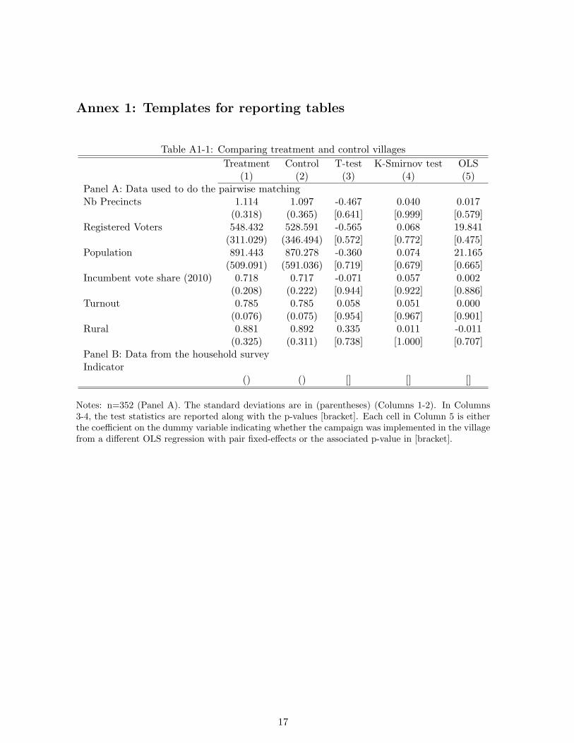
See Table A1-1 for a template and for initial results for the variables that were used to do

the pairwise matching.

5.2 Estimation Strategy

In this section, we list the regressions that we will run once the data are available. All

results will be reported in the paper. We anticipate running additional regressions during the

data analysis stage, in order to explore further the relationships that emerge from running

our registered regressions. If so, the associated results will be labelled as such in the paper

(Casey, Glennerster and Miguel 2012).5There is a risk that if voters have strong pre-intervention preferences over a candidate they might align

their preferences with the candidate’ promises. In that case, the sample might not be balanced along thosevariables. If that is the case, we will test if the distance between voter preferences and promises of theirpreferred candidate are smaller in treatment barangays than in control barangays.

6We will not necessarily control for control for variables that show a statistically significant difference inmean pre-treatment (Brunh and McKenzie 2009).

8

5.2.1 Hypothesis 1

Hypothesis 1 will be tested using individual-level data on knowledge about candidates and

their platforms. First, we will estimate the intervention’s impacts on knowledge of candidates’

promises:

Yijk = αTj + vk + uijk (1)

where Yijk is the knowledge index for individual i in village j in pair k, Tj is a dummy

equal to one if the campaign was implemented in village j, vk is a pair-specific unobservable

and, uijk is the usual idiosyncratic error term. To account for the way the randomization was

carried out standard errors will be clustered at the village level.

We will estimate equation (1) without fixed-effects, with municipal fixed effects and with

pair fixed effects (Brunh and McKenzie 2009). In addition, we will test if results are robust to

the inclusion of a number of control variables. See Table A1-2 for a template. Our preferred

specification will be the one with pair fixed effects and without additional controls.

Second, consistent with models of rational inattention, it is possible that voters will only

process information about the sectors they care most about. To test for that, we will regress

sector-specific measures of information about candidate promises, interacting the treatment

dummy with the share of budget respondents would allocate to the sector. Specifically, we

will estimate:

Yijs = αSis + βSis ∗ Tj + ws + vi + uijs (2)

where Yijs captures information individual i in village j has about candidates’ promises

on sector s, Tj is a dummy equal to one if the campaign was implemented in village j, Sis

is the share of LDF spending that individual i would want to allocate to sector s, ws is a

sector-specific unobservable and vi is a respondent-specific unobservable and uijs is the usual

idiosyncratic error term. To account for the way the randomization was carried out standard

errors will be clustered at the village level.

We will estimate equation (6) without fixed-effects, with municipal fixed effects, with pair

fixed effects and with individual fixed-effects. See Table A1-3 for a template. Our preferred

specification will be the one with individual fixed effects.

9

Third, it is possible that voters will only process the information when the differences

between the candidates’ promises are large enough. To test for that, we will regress sector-

specific measures of information about candidate promises, interacting the treatment dummy

with the gap between the top two promises in each sector. Specifically, we will estimate:

Yijs = αGjs + βGjs ∗ Tj + ws + vi + uijs (3)

where Yijs captures information individual i in village j has about candidates’ promises

on sector s, Tj is a dummy equal to one if the campaign was implemented in village j, Gjs

is the gap between the top two promises in sector s in municipality j, ws is a sector-specific

unobservable and vi is a respondent-specific unobservable and uijs is the usual idiosyncratic

error term. To account for the way the randomization was carried out standard errors will

be clustered at the village level.



specification will be the one with individual fixed effects.

Finally, to test if, as a result of the campaign, citizens are more interested in politics, we

will estimate the intervention’s impacts on political knowledge (not provided as part of the

campaign):


where Yijk is the knowledge index for individual i in village j in pair k, Tj is a dummy

equal to one if the campaign was implemented in village j, vk is a pair-specific unobservable

and, uijk is the usual idiosyncratic error term. To account for the way the randomization was

carried out standard errors will be clustered at the village level.


pair fixed effects (Brunh and McKenzie 2009). In addition, we will test if results are robust to

the inclusion of a number of control variables. See Table A1-2 for a template. Our preferred


10

5.2.2 Hypothesis 2

Hypothesis 2 will be tested using individual-level data on how salient sectoral allocations are.

Specifically, we will estimate:


where Yijk captures how salient sectoral allocations are when individual i in village j in

pair k decides which candidate to vote for, Tj is a dummy equal to one if the campaign was

implemented in village j, vk is a pair-specific unobservable and uijk is the usual idiosyncratic

error term. To account for the way the randomization was carried out standard errors will

be clustered at the village level.

As above, we will estimate equation (5) without fixed-effects, with municipal fixed effects

and with pair fixed effects (Brunh and McKenzie 2009). In addition, we will test if results

are robust to the inclusion of a number of household-level control variables. See Table A1-2

for a template. Our preferred specification will be the one with pair fixed effects and without

additional controls.

5.2.3 Hypothesis 3

Hypothesis 3 will be tested using individual-level data from the endline survey and precinct-

level data on candidate vote share. First, we will use individual-level data on support for the

various candidates’ promises and alignment between respondents’ preferences over spending

and candidates’ promises. Specifically, we will estimate:

Yijc = αAic + βTj ∗Aic + wc + vi + uijk (6)

where Yijc is a measure of the strength of individual i’s support for candidate c, Tj is

a dummy equal to one if the campaign was implemented in village j, Aic is the alignment

of individual i and candidate c preferences defined in Section 4.2, wc is a candidate-specific

unobservable, vi is a respondent-specific unobservable and uijc is the usual idiosyncratic error

term. To account for the way the randomization was carried out standard errors will be

clustered at the village level.


11



Second, we will use precinct-level data on candidate’s vote share in the 2013 elections.

Specifically, we will estimate:

Ycpjk = αTj + βAcj + γTj ∗ Acj + wc + vk + ucpjk (7)

where Ycjk is vote share for candidate c in precinct p in village j in pair k, Tj is a dummy

equal to one if the campaign was implemented in village j, Acj is the village j average

alignment with candidate’s c sectoral promises, wc is a candidate-specific unobservable, vk is

pair-level unobservable and ucjk is the usual idiosyncratic error term. To account for the way

the randomization was carried out standard errors will be clustered at the village level.

We will estimate equation (7) without fixed-effects, with municipal fixed effects, with can-

didate fixed effects and with candidate and pair fixed effects and with individual fixed-effects

(Brunh and McKenzie 2009). See Table A1-6 for a template. Our preferred specification will

be the one with candidates fixed effects and with pair fixed effects and without additional

controls.

5.2.4 Hypothesis 4

Hypothesis 4 will be tested using individual-level data from the endline survey and precinct-

level data on turnout. First, we will use individual-level data on self-reported turnout and

alignment between respondents’ preferences over spending and candidates’ promises. Specif-

ically, we will estimate:

Yijk = αBi + βTj ∗Bi + vk + uijk (8)

where Yijk is a measure of turnout for individual i, Tj is a dummy equal to one if the

campaign was implemented in village j, Bi = Maxc1,c2(Aic1 − Aic2), vk is a pair-specific

unobservable and uijk is the usual idiosyncratic error term. To account for the way the

randomization was carried out standard errors will be clustered at the village level.



12


Second, we will use precinct-level data on turnout in the 2013 elections. Specifically, we

will estimate:

Ypjk = αTj + βBj + γTjk ∗ Bj + vk + upjk (9)

where Ypjk is turnout in precinct p in village j in pair k, Tjk is a dummy equal to one

if the campaign was implemented in village j, Aj is the village j average of Bij , vk is pair-

level unobservable and ucjk is the usual idiosyncratic error term. To account for the way the

randomization was carried out standard errors will be clustered at the village level.


pair fixed effects (Brunh and McKenzie 2009). See Table A1-8 for a template. Our preferred


5.2.5 Hypothesis 5

Hypothesis 5 will be tested using village-level measures of vote-buying obtained through the

unmatched count technique, individual-level responses to direct questions about vote-buying

and, if available, field reports from PPCRV election monitors. Specifically, we will estimate:

Yjk = αTj + vk + ujk (10)

where Yjk is the prevalence of vote-buying in village j in pair k during the May 2013

elections, Tj is a dummy equal to one if the campaign was implemented in village j, vk is a

pair-specific unobservable and uijk is the usual idiosyncratic error term.

As above, we will estimate equation (10) without fixed-effects, with municipal fixed effects

and with pair fixed effects (Brunh and McKenzie 2009). In addition, we will test if results are

robust to the inclusion of a number of control variables. See Table A1-9 for a template.Our

preferred specification will be the one with pair fixed effects and without additional controls.

In our preferred specification, Yjk will be defined as the difference in the village-level

average between the count for households that were provided with a list that included vote-

buying and the count for households that were provided with a list that did not include

vote-buying.

In addition, there is evidence that in the Philippines, responses to direct question about

13

vote-buying provide credible estimates of the extent of vote-buying at the village-level (Cruz

2012). As a result, we we will also estimate equation (10) where Yjk is the village-level average

to direct questions about vote-buying. The direct questions ask respondents, first, if vote-

buying occurs in their barangay, then if the respondent was offered money or gifts in exchange

for their vote, and finally if they themselves accepted the money or gifts

5.3 Heterogeneous Effects

We will also carry out subgroup analyses and test for heterogenous effects. We will estimate

the same equations as the ones listed in Section 5.2, adding the interaction term. For con-

tinuous variables, we will interact the treatment dummy T with the demeaned variable. The

actual list of planned subgroup analyses is below:

For hypotheses that we will test using individual-level data:

• education levels

• female/male

• wealth

• level of personal connections to candidates

For all hypotheses:

• Dynastic/non-dynastic municipalities7

• levels of electoral violence

• 2010 incumbent vote share (village-level)

• 2010 turnout (village-level)

• rural/urban classification7We will use the same measure of municipal-level political dynasties as Cruz and Schneider (2012) and

Labonne (2012)

14

5.4 Potential Adjustments for non compliance and missing data

If the team is either unable to carry out the campaign or to implement they survey in a subset

of villages, they will be excluded from the analysis together with the matched pair village.

This will ensure that internal validity is preserved.

15

References

Arnold, Benjamin, Daniel Hogan, John Colford, and Alan Hubbard, “Simulation

methods to estimate design power: an overview for applied research,” BMC Medical

Research Methodology, 2011, 11 (94).

Brunh, Miriam and David McKenzie, “In Pursuit of Balance: Randomization in Practice

in Development Field Experiments,” American Economic Journal: Applied Economics,

2009, 1 (4), 200–232.

Casey, Katherine, Rachel Glennerster, and Edward Miguel, “Reshaping Institutions:

Evidence on Aid Impacts Using a Pre-Analysis Plan,” The Quarterly Journal of Eco-

nomics, 2012.

Cruz, Cesi, “Social Networks and the Targeting of Illegal Electoral Strategies,” mimeo, 2012.

and Christina Schneider, “The (Unintended) Electoral Effects of Multilateral Aid

The (Unintended) Electoral Effects of Multilateral Aid Projects,” University of Califor-

nia - San Diego, mimeo, 2012.

Kling, Jeffrey, Jeffrey Liebman, and Lawrence Katz, “Experimental Analysis of Neigh-

borhood Effects,” Econometrica, 2007, 75 (1), 83–119.

Labonne, Julien, “The Local Electoral Impacts of Conditional Cash Transfers: Evidence

from the Philippines,” Oxford University CSAE Working Paper 2012-09, 2012.

Leon, Gianmarco, “Turnout, Political Preferences, and Information: Experimental Evi-

dence from Peru,” mimeo, Universitat Pompeu Fabra, 2013.

16

Annex 1: Templates for reporting tables

Table A1-1: Comparing treatment and control villagesTreatment Control T-test K-Smirnov test OLS

(1) (2) (3) (4) (5)Panel A: Data used to do the pairwise matchingNb Precincts 1.114 1.097 -0.467 0.040 0.017

(0.318) (0.365) [0.641] [0.999] [0.579]Registered Voters 548.432 528.591 -0.565 0.068 19.841

(311.029) (346.494) [0.572] [0.772] [0.475]Population 891.443 870.278 -0.360 0.074 21.165

(509.091) (591.036) [0.719] [0.679] [0.665]Incumbent vote share (2010) 0.718 0.717 -0.071 0.057 0.002

(0.208) (0.222) [0.944] [0.922] [0.886]Turnout 0.785 0.785 0.058 0.051 0.000

(0.076) (0.075) [0.954] [0.967] [0.901]Rural 0.881 0.892 0.335 0.011 -0.011

(0.325) (0.311) [0.738] [1.000] [0.707]Panel B: Data from the household surveyIndicator

() () [] [] []

Notes: n=352 (Panel A). The standard deviations are in (parentheses) (Columns 1-2). In Columns3-4, the test statistics are reported along with the p-values [bracket]. Each cell in Column 5 is eitherthe coefficient on the dummy variable indicating whether the campaign was implemented in the villagefrom a different OLS regression with pair fixed-effects or the associated p-value in [bracket].

17

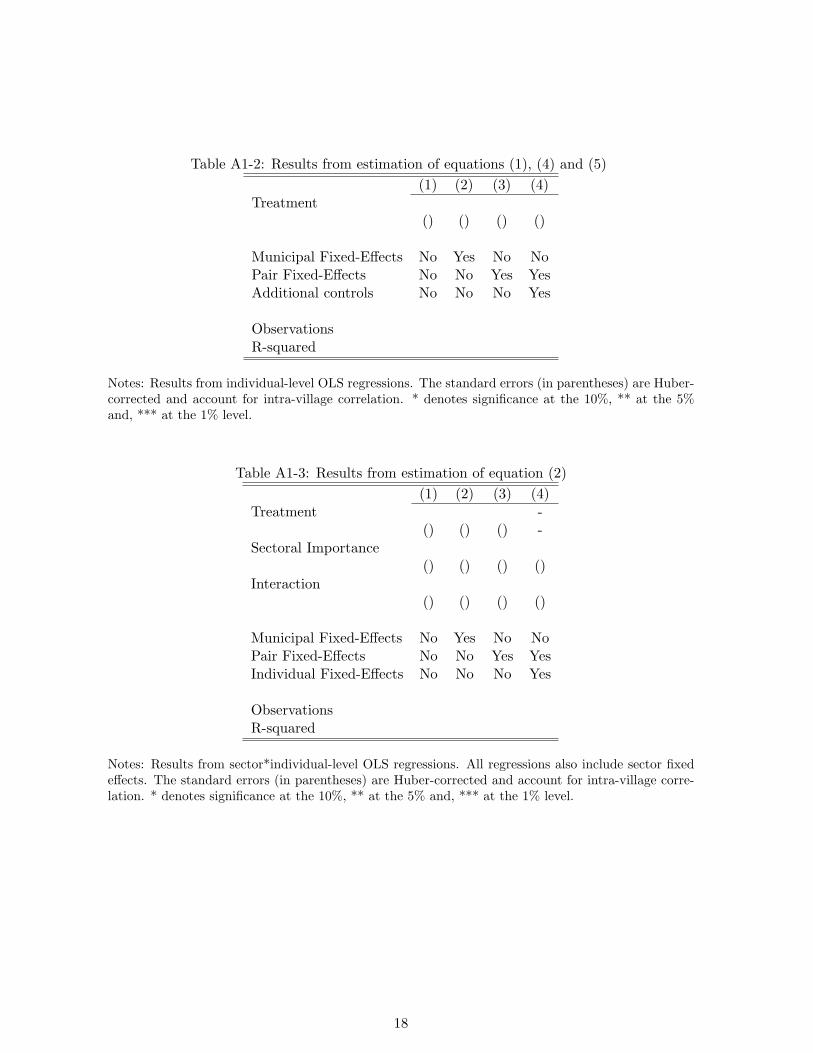
Table A1-2: Results from estimation of equations (1), (4) and (5)(1) (2) (3) (4)

Treatment() () () ()

Municipal Fixed-Effects No Yes No NoPair Fixed-Effects No No Yes YesAdditional controls No No No Yes

ObservationsR-squared

Notes: Results from individual-level OLS regressions. The standard errors (in parentheses) are Huber-corrected and account for intra-village correlation. * denotes significance at the 10%, ** at the 5%and, *** at the 1% level.

Table A1-3: Results from estimation of equation (2)(1) (2) (3) (4)

Treatment -() () () -

Sectoral Importance() () () ()

Interaction() () () ()

Municipal Fixed-Effects No Yes No NoPair Fixed-Effects No No Yes YesIndividual Fixed-Effects No No No Yes


Notes: Results from sector*individual-level OLS regressions. All regressions also include sector fixedeffects. The standard errors (in parentheses) are Huber-corrected and account for intra-village corre-lation. * denotes significance at the 10%, ** at the 5% and, *** at the 1% level.

18



Sectoral Difference() () () ()




Notes: Results from sector*individual-level OLS regressions. All regressions also include sector fixedeffects. The standard errors (in parentheses) are Huber-corrected and account for intra-village corre-lation. * denotes significance at the 10%, ** at the 5% and, *** at the 1% level.



Policy Alignment() () () ()




Notes: Results from candidate*individual-level OLS regressions. All regressions also include candidatefixed effects. The standard errors (in parentheses) are Huber-corrected and account for intra-villagecorrelation. * denotes significance at the 10%, ** at the 5% and, *** at the 1% level.

19



Policy Alignment() () () ()


Municipal Fixed-Effects No Yes No NoCandidate Fixed-Effects No No Yes NoPair Fixed-Effects No No No Yes


Notes: Results from candidate* precinct-level regressions. The standard errors (in parentheses) areHuber-corrected and account for intra-village correlation. * denotes significance at the 10%, ** at the5% and, *** at the 1% level.



Relative Preference() () () ()


Municipal Fixed-Effects No Yes No NoPair Fixed-Effects No No Yes YesVillage Fixed Effects No No No Yes


Notes: Results from individual-level OLS regressions. The standard errors (in parentheses) are Huber-corrected and account for intra-village correlation. * denotes significance at the 10%, ** at the 5%and, *** at the 1% level.

20



Relative Preference() () () ()


Municipal Fixed-Effects No Yes No NoPair Fixed-Effects No No Yes YesAdditional Controls No No No Yes


Notes: Results from precinct-level regressions. The standard errors (in parentheses) are Huber-corrected and account for intra-village correlation. * denotes significance at the 10%, ** at the 5%and, *** at the 1% level.



Municipal Fixed-Effects No Yes No NoPair Fixed-Effects No No Yes YesAdditional controls No No No Yes


Notes: Results from village-level OLS regressions. Robust standard errors (in parentheses). * denotessignificance at the 10%, ** at the 5% and, *** at the 1% level.

Annex 2: List of Intervention Municipalities

21

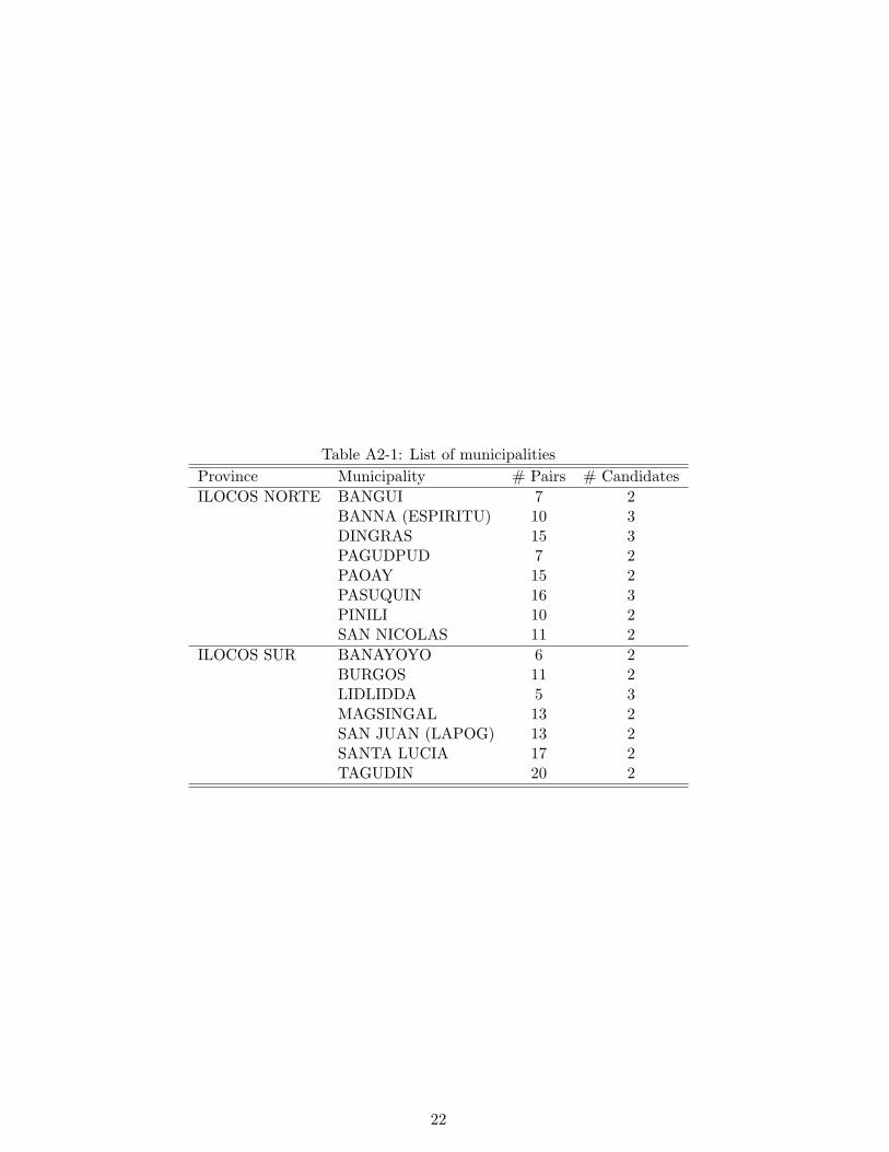
Table A2-1: List of municipalitiesProvince Municipality # Pairs # CandidatesILOCOS NORTE BANGUI 7 2

BANNA (ESPIRITU) 10 3DINGRAS 15 3PAGUDPUD 7 2PAOAY 15 2PASUQUIN 16 3PINILI 10 2SAN NICOLAS 11 2

ILOCOS SUR BANAYOYO 6 2BURGOS 11 2LIDLIDDA 5 3MAGSINGAL 13 2SAN JUAN (LAPOG) 13 2SANTA LUCIA 17 2TAGUDIN 20 2

22

Candidate Promises, Citizens Knowledge and Vote … Promises, Citizens Knowledge and Vote-Buying ......

Documents

Transcript of Candidate Promises, Citizens Knowledge and Vote … Promises, Citizens Knowledge and Vote-Buying ......