Can Volatility Solve the Naive Portfolio Puzzle?
50
Can Volatility Solve the Naive Portfolio Puzzle? * Michael Curran † Villanova University Ryan Zalla ‡ University of Pennsylvania August 6, 2020 Abstract We investigate whether sophisticated volatility estimation improves the out-of- sample performance of mean-variance portfolio strategies relative to the naive 1/N strategy. The portfolio strategies rely solely upon second moments. Using a diverse group of econometric and portfolio models across multiple datasets, most models achieve higher Sharpe ratios and lower portfolio volatility that are statistically and economically significant relative to the naive rule, even after controlling for turnover costs. Our results suggest benefits to employing more sophisticated econometric mod- els than the sample covariance matrix, and that mean-variance strategies often out- perform the naive portfolio across multiple datasets and assessment criteria. Keywords: volatility, naive portfolio, mean-variance JEL: G11, G17 * We thank Caitlin Dannhauser, Jes´ us Fern´andez-Villaverde, Alejandro Lopez-Lira, Rabih Moussawi, Michael Pagano, Nikolai Roussanov, Paul Scanlon, Frank Schorfheide, John Sedunov, Raman Uppal, and Raisa Velthuis for helpful comments. Christopher Antonello provided diligent research assistance. † Corresponding author. Email: [email protected]; Phone: (+1) 610-519-8867 Address: Economics Dept., Villanova School of Business, Villanova University, 800 E Lancaster Ave, PA 19085, USA. ‡ Email: [email protected]; Phone: (+1) 412-759-5032 Address: Economics Dept., University of Pennsylvania, 133 South 36th Street, Philadelphia, PA 19104, USA. 1 arXiv:2005.03204v2 [q-fin.GN] 4 Aug 2020
Transcript of Can Volatility Solve the Naive Portfolio Puzzle?
Can Volatility Solve the Naive Portfolio Puzzle?∗
Michael Curran†
Villanova University
Ryan Zalla‡
University of Pennsylvania
August 6, 2020
Abstract
We investigate whether sophisticated volatility estimation improves the out-of-
sample performance of mean-variance portfolio strategies relative to the naive 1/N
strategy. The portfolio strategies rely solely upon second moments. Using a diverse
group of econometric and portfolio models across multiple datasets, most models
achieve higher Sharpe ratios and lower portfolio volatility that are statistically and
economically significant relative to the naive rule, even after controlling for turnover
costs. Our results suggest benefits to employing more sophisticated econometric mod-
els than the sample covariance matrix, and that mean-variance strategies often out-
perform the naive portfolio across multiple datasets and assessment criteria.
Keywords: volatility, naive portfolio, mean-variance
JEL: G11, G17
∗We thank Caitlin Dannhauser, Jesus Fernandez-Villaverde, Alejandro Lopez-Lira, Rabih Moussawi, Michael Pagano,
Nikolai Roussanov, Paul Scanlon, Frank Schorfheide, John Sedunov, Raman Uppal, and Raisa Velthuis for helpful comments.
Christopher Antonello provided diligent research assistance.†Corresponding author. Email: [email protected]; Phone: (+1) 610-519-8867
Address: Economics Dept., Villanova School of Business, Villanova University, 800 E Lancaster Ave, PA 19085, USA.‡Email: [email protected]; Phone: (+1) 412-759-5032
Address: Economics Dept., University of Pennsylvania, 133 South 36th Street, Philadelphia, PA 19104, USA.
1
arX
iv:2
005.
0320
4v2
[q-
fin.
GN
] 4
Aug
202
0
CAN VOLATILITY SOLVE THE NAIVE PORTFOLIO PUZZLE? 1
1 Introduction
Ever since mean-variance strategies were introduced by Markowitz (1952), their out-of-
sample performance has been criticized. One reason for weak performance is estimation
error, particularly in the mean return (Merton, 1980; Chopra and Ziemba, 2013). Variance
strategies, which rely solely upon second moments, avoid the pitfall of expected returns es-
timation. In comparing variance strategies relative to the naive 1/N portfolio benchmark,
while the portfolio selection literature advocates robust estimation procedures to reduce
estimation error, previous work such as DeMiguel et al. (2009b) include strategies account-
ing for parameter errors, but employ sample covariance estimates. Few papers in the naive
portfolio literature pursued improved estimation of the volatility of returns.1,2 Our marginal
contribution is that a variety of econometric models of volatility improve performance rel-
ative to the naive portfolio strategy. That is, relative to sample covariance estimation, our
study suggests considerable performance gains from employing modern econometric models
for estimating volatility in portfolio construction.
We investigate whether sophisticated volatility estimation improves the performance of
mean-variance strategies depending only on conditional variance-covariance matrices (vari-
ance strategies) relative to the naive 1/N strategy. Using a diverse set of fourteen econo-
metric models, we evaluate the out-of-sample performance of portfolio strategies that rely
solely on estimation of the second moment of returns. We apply three portfolio strategies
1Instead of the portfolio strategy, our innovation explores a wide variety of econometric models.DeMiguel et al. (2009b) find that the minimum-variance portfolio, though performing well relative to otherportfolio strategies, significantly beats the 1/N strategy for only 1 in 7 of their datasets. Jagannathanand Ma (2003) and Kirby and Ostdiek (2012) innovate on the portfolio model, illustrating that short-saleconstrained minimum-variance strategies and volatility timing strategies enhance performance.
2We consider a wide range of mostly parametric econometric models. Non-parametric models usinghigher-frequency data (DeMiguel et al., 2013) and shrinkage approaches (Ledoit and Wolf, 2017) alsoimprove the accuracy of estimation. Daily frequency option-implied volatility reduces portfolio volatility,but never statistically significantly improves the Sharpe ratio relative to the 1/N strategy (DeMiguel et al.,2013). Initial investigations reveal our results to be at least as strong as Ledoit and Wolf (2017).
2 CURRAN AND ZALLA
– minimum-variance, constrained minimum-variance, and volatility-timing – to six empir-
ical datasets of weekly and monthly returns; we also include the tangency portfolio.3 We
assess performance using the following three criteria: (i) the Sharpe ratio, (ii) the turnover
(trading) costs, and (iii) the standard deviation of returns (portfolio volatility). Overall,
we show that variance strategies perform consistently and significantly well out-of-sample.
Our first contribution is to show that all four portfolio strategies, regardless of the econo-
metric model used for estimating covariance, achieve improved out-of-sample performances
relative to the naive benchmark. This assertion challenges the literature that has rarely re-
ported superior minimum-variance performances relative to the equally-weighted portfolio
(DeMiguel et al., 2009b).4 Specifically, we find that all four portfolio strategies estimated
using all fourteen econometric models perform at least as well as the naive benchmark,
and only rarely underperform it. These underperformances are mainly concentrated in the
Fama-French 3-factor dataset. If we discard this dataset, then all four portfolio strategies
estimated using twelve of the fourteen econometric models would not just perform well,
they would weakly dominate the naive benchmark.5
In general, the minimum-variance strategy, with or without short-sale constraints, achieves
higher Sharpe ratios, lower turnover costs, and lower portfolio volatility across the majority
of datasets. Wherever these strategies do not perform significantly better than the naive
rule, we often fail to reject the null hypothesis that their performances are identical to
the naive rule. Likewise, we find evidence that volatility-timing strategies achieve higher
Sharpe ratios and lower turnover costs but exhibit portfolio volatility that is comparable
to the naive rule. The tangency portfolio does reasonably well in certain datasets. Rela-
3Section 3 defines our financial portfolio models.4Our econometric estimation strategies yield improvements beyond the period and frequency differences.5A portfolio strategy, whose covariance is estimated using a given econometric model, weakly dominates
the naive benchmark if, for each performance criterion, the portfolio strategy performs at least as well asthe naive benchmark across all datasets and performs significantly better in at least one dataset.
CAN VOLATILITY SOLVE THE NAIVE PORTFOLIO PUZZLE? 3
tive to the other strategies, however, its performance is lackluster, which we attribute to
estimation error in expected returns.
Our second contribution is to identify pairings of volatility models and portfolio strate-
gies that perform consistently and significantly well across datasets relative to the naive
benchmark. Multivariate GARCH models, particularly the constant conditional correla-
tion (CCC), weakly dominate the naive rule when applied to minimum-variance and con-
strained minimum-variance strategies. Similarly, the realized covariance (RCOV) model
weakly dominates the naive rule when applied to the volatility-timing strategy. In the
tangency portfolio, although the RCOV model achieves higher Sharpe ratios and lower
portfolio volatility relative to the naive strategy than other econometric models, it ex-
hibits higher portfolio volatility relative to the naive rule in data on international equities.
Thus, although we cannot say the RCOV model applied to the tangency portfolio weakly
dominates the naive rule, many other econometric models do, such as the multivariate
GARCH models. Nonetheless, even econometric models such as the regime-switching vec-
tor autoregression (RSVAR) and exponentially-weighted moving-average (EWMA), which
perform worst in each of the four porfolio models, still perform at least as well as the naive
benchmark across every dataset except the Fama-French 3-factor.
Our third contribution is to compare the performance of econometric models relative to
the naive benchmark using each assessment criterion in isolation. That is, across portfolios
models and datasets, which econometric models consistently achieve the highest Sharpe
ratios? Which econometric models achieve the lowest turnover costs? Which econometric
models achieve the lowest portfolio volatilities? First, the combined parameter (CP) and
realized covariance (RCOV) models achieve significantly higher Sharpe ratios than the naive
benchmark. Second, the RCOV and a variety of GARCH models produce significantly
higher Sharpe ratios than the naive rule after adjustment for turnover costs. Finally, the
4 CURRAN AND ZALLA
exponentially-weighted moving-average (EWMA), multivariate stochastic volatility (MSV),
and RCOV models exhibit significantly lower portfolio volatility than the naive rule. These
performances are economically and statistically significant: relative to the naive strategy,
we achieve 30% higher Sharpe ratios and 9% lower portfolio volatility.6
Our paper exploits recent computational developments to estimate the covariance ma-
trix using multivariate, nonlinear, non-Gaussian econometric models. We extend the set
of models in Wang et al. (2015) beyond GARCH and discrete regime-switching models
to smooth multivariate stochastic volatility and non-parametric realized volatility models.
Unlike Wang et al. (2015), our models employ multivariate (N ≈ 10) rather than bivariate
(N = 2) sets of assets. Our study benefits from incorporating recent advances in the compu-
tation of several models as in Vogiatzoglou (2017), Chan and Eisenstat (2018), and Kastner
(2019b).7
We draw two conclusions from our results. First, relative to sample covariance estima-
tion, our study suggests considerable performance gains from employing modern economet-
ric models for estimating volatility in portfolio construction. Second, variance strategies
consistently perform well relative to the naive strategy.
To place our paper in context, our study builds on the literature of naive diversification.
Mean-variance models struggle to compete with naive diversification in out-of-sample return
performance. Considering a variety of mean-variance strategies including ones accounting
for parameter errors, DeMiguel et al. (2009b) find that no portfolio model consistently
outperforms naive diversification. One cause for the weak performance is that while mean-
variance strategies based on the minimum-variance portfolio outperforms naive diversifica-
6For each portfolio strategy, we average the Sharpe ratios and portfolio volatility resulting from allfourteen econometric models across all six datasets. Then we average Sharpe ratio and portfolio volatilityacross all four portfolio models.
7To reduce run-time, we employ fast, low-level languages, e.g., C++, that we program in parallel withhyperthreading and execute on clusters.
CAN VOLATILITY SOLVE THE NAIVE PORTFOLIO PUZZLE? 5
tion, portfolio turnover costs negates these benefits (Kirby and Ostdiek, 2012). To address
the turnover issue, the authors propose two new approaches that reduce portfolio turnover,
finding that the mean-variance strategies outperform the naive strategy out-of-sample. We
employ their volatility-timing strategy. Combining naive diversification with other con-
ventional portfolio strategies can also significantly enhance portfolio performance (Tu and
Zhou, 2011). We investigate combining parameters from the variance-covariance matrix
estimates as well as from the weights suggested by portfolio models.
A number of studies have increased the sophistication of parameter estimation since
DeMiguel et al. (2009b), which was based on rolling window sample estimates. Considering
a variety of mostly GARCH-based estimators, no method is universally superior (Trucıos
et al., 2019).8 A non-linear shrinkage estimator (Ledoit and Wolf, 2017) and an estimation
strategy for large portfolios (Ao et al., 2019) can improve performance.9 The use of implied
volatility and skewness (DeMiguel et al., 2013), vector autoregression (DeMiguel et al.,
2014), and portfolio constraints (DeMiguel et al., 2009a; Kourtis et al., 2012; Behr et al.,
2013) also enhances portfolio performance.10 Recent papers find comparably poor perfor-
mance using sophisticated hedging strategies to attempt beating naive one-to-one hedg-
ing (Wang et al., 2015), provide behavioral evidence of naive choice strategies (De Giorgi
and Mahmoud, 2018; Gathergood et al., 2019), and identify the importance of volatility
for portfolio performance (Moreira and Muir, 2017, 2019). Consistent with Moreira and
8Using a shorter time-sample across one dataset with a larger portfolio, they do not consider vectorautoregression, vector error correction for non-stationarity, or either regime-switching or stochastic volatilitymodels, which are computationally challenging and account for observed nuances of time-varying volatility.
9Preliminary evidence suggests that our results are at least as strong relative to the naive portfolio aswhat Ledoit and Wolf (2017) find. Direct comparisons are more complicated in Ao et al. (2019). Relativeto the naive portfolio, initial experiments suggest that their MAXSER estimator performs better than oureconometric models do in some comparisons, but that our models do better in most empirical comparisons.
10To isolate one study by DeMiguel et al. (2009a), our paper employs improved econometric methodsrather than more sophisticated portfolio constraints. Although not directly comparable, preliminary in-vestigations reveal that our models improve performance relative to the naive portfolio by a greater ratiothan DeMiguel et al. (2009a) in terms of Sharpe ratios, portfolio volatility, and turnover costs.
6 CURRAN AND ZALLA
Muir (2017, 2019), our paper finds that volatility-timing strategies generate higher Sharpe
ratios in these same datasets yet exhibit equal volatility to the naive portfolio. Taking
seriously the naive strategy as an important benchmark, we explore improved econometric
estimation of volatility as a potential source of out-of-sample performance.
Our benchmark is the naive portfolio diversification rule, allocating a fraction 1/N of
wealth to each of N assets available for investment at each rebalancing date.11 Three
reasons justify the naive rule as a benchmark. First, implementation is easy as it relies
on neither optimization nor estimation of the moments of asset returns. Second, investors
use such simple rules for allocating their wealth across assets (Benartzi and Thaler, 2001;
Baltussen and Post, 2011; De Giorgi and Mahmoud, 2018; Gathergood et al., 2019). Third,
the naive rule consistently outperforms mean-variance strategies (Jobson and Korkie, 1980;
Michaud and Michaud, 2008; DeMiguel et al., 2009b; Duchin and Levy, 2009; Pflug et al.,
2012). Without needing to estimate the 1/N weights, the variance of parameter estimation
is zero, and thus the mean square error of the naive portfolio weights is simply the square
of the bias.12 The naive strategy therefore proxies as a challenging rival for mean-variance
strategies to outperform.
11We apply our methods to six different empirical datasets with N ≤ 11 portfolio choices. In preliminaryinvestigations, we experimented with datasets withN = 25 portfolio choices. As indicated by DeMiguel et al.(2009b), however, the critical minimal value for the estimation period (rolling window sample) grows in N ,requiring windows much larger than 10 years. Larger N reduces performance when the estimation windowis fixed. The reason is that there are more parameters in the covariance matrix to estimate and thereforethere is more room for estimation error. Large portfolio choice sets preclude using most empirical datasetsbecause we typically need over 100 years of data. Employing larger datasets also significantly increases thecomputing time. Fortunately, our multiple datasets are broad and varied. For instance, we cover datasetsallowing investors to diversify across international equities in the form of national stock market aggregateindices, across entire sector and industry indices, across expansive Fama-French portfolios, and across otherencompassing indices based on size/book-to-market and momentum portfolios. The best application forour methods from a practical standpoint, therefore, is to an investor holding multiple mutual funds inequities.
12Letting w denote our estimate of the optimal vector of portfolio weights w, the MSE bias-variancedecomposition from econometrics is MSE(w) = V ar(w) +Bias2(w,w), where Bias(w,w) = w −w.
CAN VOLATILITY SOLVE THE NAIVE PORTFOLIO PUZZLE? 7
2 Econometric Models
Table 1 lists the econometric models, some of which are included in Wang et al. (2015), who
consider out-of-sample performance of hedging strategies.13 Their analysis uses econometric
modeling of bivariate random variables, whereas we extend the analysis to multivariate
random variables, where N > 2. We use a rolling window approach with T +M returns for
N assets. M is the estimation window length so that there are T out-of-sample investment
periods. Picking ten-year rolling windows, M will be set by the frequency of the data.
For instance, M = 520 for weekly data and M = 120 for monthly data. We choose T = 1,
which corresponds to one week or month ahead, reduces compute time, and allows us to
compare our results with the literature, e.g., DeMiguel et al. (2009b). Let {Σjt}Tt=1 denote
the conditional estimate of the variance-covariance matrix of returns for investment period t
based on econometric model j. Similarly, we define the conditional estimate of the expected
return over period t given model j by {µj}Tt=1. The portfolio models we focus on are based
solely on the variance-covariance matrix. We also experiment with the tangency portfolio
and use the sample mean, which is independent of econometric model j, as our estimate of
the mean. Mean-variance strategies are defined by the first two conditional moments of the
return for period t so that {(µjt , Σ
jt)}Tt=1 defines the sequence of mean-variance strategies
over the T out-of-sample investment periods with respect to model j. Section 3 details the
mean-variance strategies.
2.1 Sample Covariance
Our first econometric model to estimate the variance-covariance matrix is the sample covari-
ance matrix (Cov). Sample-based in-sample estimation of the variance-covariance matrix
13While we attempt to cover the broad classes of econometric models, our set of econometric models isnot exhaustive. For instance, we omit the shrinkage estimators of Ledoit and Wolf (2003, 2017). Althoughthese and other econometric models are interesting, we exclude them in the interest of space.
8 CURRAN AND ZALLA
is standard in the literature on the naive diversification puzzle (DeMiguel et al., 2009b;
Fletcher, 2011; Tu and Zhou, 2011; Kirby and Ostdiek, 2012). Some studies examine im-
proved estimation, but they typically focus on a small set of models (DeMiguel et al., 2013).
The sample covariance matrix places equal weight on past observations.
2.2 Exponentially Weighted Moving Average
The recent past might be more informative for estimating the variance-covariance matrix
to use in selecting portfolios, motivating our first refinement, the exponentially weighted
moving average (EWMA) model. The EWMA model suggested by RiskMetrics places
decaying weight on the past: Σt = αΣt−1+(1−α)(rt− rt)′(rt− rt) where our decay parameter
suggested is 0.96 (weekly) or 0.97 (monthly).
2.3 Vector Autoregression
To exploit dependence along the cross-section and time-dimension (serial), we estimate
a vector autoregression (VAR): Y = XΦ + U using Bayesian methods. We experimented
with a VAR with a Normal-Wishart natural conjugate prior and another with a Minnesota
prior. To reduce the impact of our prior on our results, we choose the posterior based on a
non-informative prior, and we report the posterior mode of the variance-covariance matrix.
Long lags are helpful to approximate the Wold representation, but we typically find two
lags to be optimal at weekly and monthly frequencies, especially as we look at financial
variables and given computational considerations. We therefore include a constant and two
lags of the variables, i.e., we estimate a VAR(2).
2.4 Vector Error Correction
Accounting for potential cointegration between the variables, we move beyond VAR to
estimate a parsimonious vector error correction (VEC) model: ∆yt = Πyt−1+∑p−1i=1 Φ∗
i ∆yt−i+
εt. We compute the number of cointegrating relations in the system following the Johansen
CAN VOLATILITY SOLVE THE NAIVE PORTFOLIO PUZZLE? 9
trace test (Johansen, 1988, 1991) and employ the variance-covariance matrix estimated from
the VEC model. If the Johansen test fails to reject the null of no cointegrating relations,
then our VEC reduces to a VAR in first differences (error-correction coefficient is zero).
2.5 BEKK-GARCH and Asymmetric BEKK-GARCH
The volatility of financial return data varies over time. General Autoregressive Condi-
tional Heteroscedasticity (GARCH) provides a simple way of modeling the evolution of
volatility as a deterministic function of past volatility and innovations. Univariate GARCH
expresses the error term of a time series εt = H1/2t ξt where ξt is an i.i.d. innovation and
Ht = f({εt−i,Ht−j}q,pi=1,j=1) and can be extended to the multivariate setting through the
vech(⋅) operator that stacks the lower triangular part of a symmetric N ×N matrix into a
N∗ = N(N+1)/2 dimensional vector: vech(Ht) = ω+∑qi=1Aiηt−i+∑
pj=1Bjht−j. With this no-
tation, ht = vech(Ht), ω is the constant component of the covariances, and ηt = vech(εtεTt ).
To prepare the data for GARCH estimation, we fit an ARMA model to the data for each
series from which to obtain demeaned residuals εt. Diagnostics such as Ljung Box tests of
serial correlation suggest ARMA(1,1) fits the data well.
Our first multivariate GARCH specification is BEKK-GARCH (Engle and Kroner,
1995), which allows for the dependence of conditional variances of one variable on lagged
values of another so that causalities in variances can be modeled. Empirically, BEKK is gen-
eral, but easy to estimate. Relaxing symmetry, we also allow positive and negative shocks of
equal magnitude to have different effects on conditional volatility by employing Asymmetric
BEKK (ABEKK). With ABEKK, vech(Ht) = ω +∑qi=1 [Aiεt−i +Ciηt−i] +∑
pj=1Bjht−j. We
allow (q = 1) one symmetric innovation when estimating BEKK. When estimating ABEKK,
we allow one symmetric innovation and one asymmetric innovation.
10 CURRAN AND ZALLA
2.6 Conditional Correlation: Constant, Dynamic, & Asymmetric
BEKK and its sibling ABEKK suffer from the curse of dimensionality that might render
them computationally infeasible for investors allocating capital across a large set of assets.
We therefore also estimate a constant conditional correlation (CCC) model. The CCC
model is a multivariate GARCH model, where all conditional correlations are constant and
conditional variances are modeled by univariate GARCH processes (Bollerslev et al., 1990).
Let us decompose the conditional covariance matrix into conditional standard deviations
and a correlation matrix Ht =DrRtDt where Dt = diag (h1/21t , . . . , h
1/2Nt ) is a diagonal matrix
of the standard deviations for the N assets. The conditional correlation matrix for the CCC
model is constant over time: Rt = R. The CCC model benefits from almost unrestricted
applicability for large systems of time series, but fails to account for the observation that
correlation increases during financial crises.
Dynamic conditional correlation (DCC) permits correlation to vary over time (Engle,
2002). In addition to DCC, we also estimate its asymmetric version (ADCC). Without ac-
counting for dynamics of asymmetric effects, DCC cannot distinguish between the effect of
past positive and negative shocks on the future conditional volatility and levels (Cappiello
et al., 2006). As when we estimate BEKK and ABEKK, we allow (q = 1) one symmet-
ric innovation when estimating CCC and DCC. When estimating ADCC, we allow one
symmetric innovation and one asymmetric innovation.
2.7 Copula-GARCH
The assumption of multivariate normality is often called into question in practical applica-
tions. As motivation, consider Apple and Microsoft, who produce similar products. Shocks
that affect Apple may be expected to affect Microsoft. Each company may experience sim-
ilar nonlinear extreme events, hence exhibiting tail dependence. A portfolio manager who
CAN VOLATILITY SOLVE THE NAIVE PORTFOLIO PUZZLE? 11
assumes multivariate normality will underestimate the frequency and magnitude of rare
events. Such underestimation may be detrimental to the performance of the portfolio.
Modeling multivariate dependence among stock returns without assuming multivariate
normality has become popular in the 21st century. Copulas are functions that may be used
to bind univariate marginal distributions to produce a multivariate distribution (Sklar,
1959). Parameters can vary over time as an autoregression in a copula-GARCH model.
Copulas have become the standard tools for modeling multivariate dependence among stock
returns without assuming multivariate normality with many general applications in finance
(Stric and Granger, 2005; Zimmer, 2012; Christoffersen et al., 2012; Aloui et al., 2013;
Christoffersen and Langlois, 2013; Creal et al., 2013; Xiao, 2014; Adrian and Brunnermeier,
2016; Bodnar and Hautsch, 2016; Solnik and Watewai, 2016; Bekiros et al., 2017).
We specify a copula-GARCH process without fitting a VAR for the conditional mean.
We set the following tuning parameters to the robust regression: γ = 0.25 (proportion to
trim), δ = 0.01 (critical value for the re-weighted estimator), 500 subsets, and 10 steps.
We allow for a symmetric DCC autoregressive order of (1,1) and choose the multivariate
Student copula distribution model, where the DCC copula is static, and we estimate the
correlation parameter in the static Student copula by maximum likelihood. We apply an
empirical (pseudo maximum likelihood) transformation to the marginal innovations of the
GARCH fitted models. In estimating the above specification for return data, we calculate
standard errors, require stationarity when optimizing the univariate GARCH, and do not
use any scale option during this first stage.14 We take the average robust estimate of the
14We alternate between using R’s solnp solver, which is a nonlinear optimization using the augmentedLagrange method, and gosolnp, which randomly initializes and conducts multiple restarts of the solnpsolver. When the objective function is non-smooth or has many local minima, it is hard to judge theoptimality of the solution, and this usually depends critically on the starting parameters. The gosolnpfunction enables the generation of a set of randomly chosen parameters from which to initialize multiplerestarts of the solver. We chose solnp, as it is faster, but when our solver encounters difficulties, we switchto gosolnp.
12 CURRAN AND ZALLA
covariance matrix.
2.8 Regime-Switching Vector Autoregression
To account for bull and bear phases of the market, we estimate a discrete time-varying
parameter model in the form of a regime-switching VAR (RSVAR) as in Chan and Eisenstat
(2018): B0,Styt = µSt+B1,Styt−1 + ⋯ +Bp,Styt−p + εt where εt ∼ N (0,ΣSt). We choose two
regimes. For each rolling window, we use a pre-sample of one year and estimate over the
remaining sample of nine years in the window. Our Bayesian estimation includes 20,000
simulations with a burn-in of 5,000 periods. We set our lag length at 2 for parsimony.
To derive the variance-covariance matrix from the RSVAR, we back out the states using
highest probability, get part of the parameter set Θ corresponding to the state at each time,
and calculate the variance-covariance matrix as Σ = (Y −XΘ)′(Y −XΘ).
2.9 Multivariate Stochastic Volatility
Another nonlinear state-space model that allows for heteroscedasticity is the computation-
ally challenging multivariate stochastic volatility model (MSV). The curse of dimensionality
for the MSV is that the degrees of freedom in the variance-covariance matrix scales quadrat-
ically with the number of assets. Multivariate factor stochastic volatility breaks the curse
of dimensionality by decomposing the variance-covariance matrix and using the pivoted
Cholesky algorithm of Higham (1990). The decomposition transforms the estimation prob-
lem from being quadratic in assets to becoming linear in assets.15
We demean the data and use r = 2 factors, where the factor loadings are unidentified.
As the sampler places no constraints on the loading matrix, we benefit from significant
15We adapt our method and exposition from Kastner (2019a,b). Observations of returns yt =(yt1, . . . , ytN)′ follow
yt∣Λ, ft, Σt ∼ NN(Λft, Σt)ft∣Σt ∼ N (0, Σt),
CAN VOLATILITY SOLVE THE NAIVE PORTFOLIO PUZZLE? 13
reductions in run time.16 Placing no constraints on the loading matrix possibly results
in unstable posteriors or multiple local optima. The instability of posterior estimates or
multiplicity of local optima cause no issues for our study, however, as inference is on the
covariance matrix rather than on the factor loadings (Kastner, 2019a). We find 10,000
draws with a burn in of 1,000 sufficient for convergence of the estimates.
2.10 Realized Volatility
Our final econometric model is a non-parametric model: realized volatility (RCOV). Re-
alized variance is the summation matrix of the return vector outerproduct r′iri over each
day in a given week for weekly frequency analysis or over each day in a given month for
monthly frequency analysis. Realized volatility is the Cholesky decomposition of the re-
alized variance. We focus on annualized realized volatility by pre-multiplying the realized
variance by the number of trading days in a year divided by the number of trading days
in a week for weekly frequency analysis or in a month for monthly frequency analysis and
obtaining the Cholesky decomposition of this product.
where ft = (ft1, . . . , ftr)′ is the vector of factors and Λ ∈ RN×r is the matrix of factor loadings. Thecovariance matrices Σt and Σt are diagonal and represent stochastic volatility processes
Σt = diag(exp ht1, . . . , exp htN)Σt = diag(exp ht1, . . . , exp htr)hti ∼ N (µi + ψi(ht−1,i − µi), σ2
i ) i = 1, . . . ,N
htj ∼ N (µj + ψj(ht−1,j − µj), σ2j ) j = 1, . . . , r.
With latent factor models, few shocks drive the system and we can reduce the number of unknowns throughthe decomposition Σt = Σt + Σt where rank(Σ) = r < N and Σt is a diagonal matrix where the diagonalentries are the idiosyncratic errors. Using the pivoted Cholesky algorithm of Higham (1990), Σt = ΨΨ′
where Ψ ∈ RN×r has Nr − r(r − 1)/2 free elements; therefore, N(r + 1) − r(r − 1)/2 free elements are left inΣt, which is now linear in N . Thus, Σt = ΛΣtΛt + Σt.
16We also speed up computation by storing only the conditional covariance matrix and the square rootsof its diagonal elements and parallelizing the factorstochvol function of Kastner (2019a) in R and C++with hyperthreading.
14 CURRAN AND ZALLA
3 Portfolio Models
Table 2 details the portfolios we compare. In order to avoid the significant issues with
estimating mean returns (Merton, 1980) and the relatively large impact of errors in the
mean vector on out-of-sample portfolio performance (Chopra and Ziemba, 2013), we choose
to concentrate on portfolio models that depend only on the covariance matrix.
3.1 Naive Diversification
With N assets, the portfolio held over investment period t, wNVt , is given by
wNVt = (1/N, . . . ,1/N) ∀t. (1)
3.2 Minimum-Variance Portfolio
The minimum-variance portfolio for investment period t, wMV Pt , minimizes conditional
portfolio variance. For each econometric model j discussed in Section 2, we calculate the
minimum-variance portfolio by
wMV Pt,j = argmin
w∈RN ∣w′1=1wΣj
tw′. (2)
For each econometric model, the conditional estimate of the covariance matrix over period
t is used as an input to find the minimum-variance portfolio.
3.3 Constrained Minimum-Variance Portfolio
The constrained minimum-variance portfolio for investment period t, wCon−MV Pt , minimizes
conditional portfolio variance subject to no short selling, which has been shown to improve
performance (Jagannathan and Ma (2003); DeMiguel et al. (2009b)). For each econometric
CAN VOLATILITY SOLVE THE NAIVE PORTFOLIO PUZZLE? 15
model j discussed in Section 2, we calculate the minimum-variance portfolio by
wCon−MV Pt,j = argmin
w∈RN ∣w′1=1,w≥0
wΣjtw
′. (3)
For each econometric model, we use the conditional estimate of the covariance matrix over
period t as an input to find the constrained minimum-variance portfolio.
3.4 Volatility-Timing Strategies
The volatility-timing strategy ignores off-diagonal elements of the covariance matrix, i.e.,
assumes all pair-wise correlations are zero (Kirby and Ostdiek, 2012). The minimum-
variance portfolio given covariance matrix Σ is wV Ti = 1/Σii
∑Ni=1 1/Σii
. We similarly define the
volatility-timing (VT) strategy given conditional estimate of the covariance matrix Σjt by
(wV Tt,j )
i=
1/ (Σjt)i,i
∑Ni=1 1/ (Σj
t)i,ii = 1, . . . ,N. (4)
3.5 Tangency Portfolio
While our main focus is on minimum-variance portfolio strategies, we also include the
tangency portfolio (TP) for illustrative purposes. The TP with respect to econometric
model j, wTPt,j , is given by
wTPt,j = argmax
w∈RN ∣w′1=1
wµjt
wΣjtw
′. (5)
3.6 Combined Parameter Model
We combine portfolios by inputting the arithmetic average over the econometric estimates
of the covariance matrix into the portfolio optimization strategies. We form a combined
parameter estimate of the covariance matrix Σ by equally weighting over estimates of
the covariance matrix taken from each of the thirteen econometric models. We use the
16 CURRAN AND ZALLA
combined parameter estimate for Σ in each of (2)–(5) to get four combined parameter
portfolios. Taking the example of the minimum-variance portfolio, using Σcomv as the
arithmetic average of the covariance matrices across the thirteen econometric models, our
combined portfolio strategy is
wMV P,comvt,j = argmin
w∈RN ∣w′1=1wΣcomv
t w′. (6)
Our combined parameter model is motivated by the finding that combining different hedging
forecasts leads to more consistent hedging performance across datasets (Wang et al., 2015).
The result echoes the forecasting literature finding that combined models tend to perform
more consistently over time than individual models (Stock and Watson, 2003, 2004).
In preliminary investigations, we explored two other approaches: (i) naively weighting
across the thirteen vectors of weights suggested by the portfolio model using each econo-
metric model’s variance-covariance matrix estimate as an input; and (ii) naively weighting
across the four weights suggested by the four financial portfolio models for a given econo-
metric model.17 These alternative combined parameter models are less relevant for our
17First, a variation of our benchmark combined parameter model (6), for each of the financial portfoliomodels (2)–(5), we examine the corresponding portfolio given by naive investments across the thirteenportfolios with respect to each of the econometric models. More precisely, consider the minimum-varianceportfolio. We form a fourteenth portfolio strategy, wMV P,com
t , which is equally invested across the thirteenestimates of the true minimum-variance portfolio, i.e.,
wMV P,comt = 1
13
13
∑j=1
wMV Pt,j .
Second, with respect to each of the econometric models, we examine the corresponding portfolio givenby naive investments across the four financial portfolio models (2)–(5). More precisely, consider the VAR
econometric model. We form a fifth portfolio strategy, wV AR,compt that is equally invested across the
four vectors of portfolio weights suggested by inputting the volatility estimates from the VAR model intofinancial portfolio strategies (2)–(5), i.e.,
wV AR,compt = 1
4
4
∑k=1
wkt,V AR.
CAN VOLATILITY SOLVE THE NAIVE PORTFOLIO PUZZLE? 17
study. With the first variation, averaging over thirteen weights suggested by the portfolio
model is less direct than averaging over the variance-covariance matrix estimates. With
the second variation, averaging over four portfolio models for a given econometric model is
similar to that of Wang et al. (2015). Consider instead the realistic situation that we are
unsure of the data generating process underlying the return series. Rather than choosing
one econometric model, we benefit from using all the information by hedging equally across
the various nuances captured by each of the thirteen econometric models. Results are
broadly similar across the three versions of combined parameter models. Thus, we report
the results from our combined parameter model (6), which we denote CP.
4 Data
We employ six datasets at weekly and monthly frequencies. Lower frequencies smooth
out too much volatility, and thus, are inappropriate for our study. Higher frequencies are
computationally infeasible in light of estimating some of our econometric models using
rolling windows with the length and frequency of our samples. Comparisons could thus be
made only for a subset of our econometric models.18 We use value-weighted returns and
assess robustness to equally-weighted returns. We use end of period data where possible.
When weekly or monthly frequency is unavailable, we scale data geometrically. For instance,
to scale returns from daily to weekly frequency, we use ΠNDj=1 (1 + rj)1/ND − 1 where rj is the
daily return and ND denotes the number of trading days in the week. We adopt similar
procedures to scale to monthly frequency. For the realized covariance (RCOV) model, we
use daily data to calculate RCOV over each week for weekly frequency analysis and over
each month for monthly frequency analysis. We omit data prior to July 1963.19
18Higher frequency data generate more accurate estimates of the covariance matrix, relevant for ourstudy, but daily and higher frequency data are also troubled with the problem of asynchronous trading.
19Standard and Poor’s established Compustat in 1962 to serve the needs of financial analysts and back-filed information only for the firms that were deemed to be of the greatest interest to the analysts. The
18 CURRAN AND ZALLA
Our first four datasets closely correspond to datasets 4, 2, 1, and 3 of DeMiguel et al.
(2009b). The authors suggest minimum critical values for the size of the estimation window
that allow these strategies to beat the naive portfolio. We choose datasets with a small
number of assets (N ≈ 10) because the minimum critical value grows with the number of
assets. Large estimation windows reduce the number of out-of-sample periods and become
unrealistic with most weekly and monthly frequency empirical datasets for N > 25. We also
motivate this choice because of computational considerations.20 Rather than examining
simulated datasets, such as randomized selections of stocks, we restrict our attention to
empirical datasets because our focus is on the econometric model as the source of improve-
ment in performance.
4.1 Dataset 1: Fama-French Portfolios
Our first dataset consists of returns obtained from Wharton Research Data Services.21 We
focus on the three-factor Fama-French portfolio: Small Minus Big, High Minus Low, and
Market portfolios. Small Minus Big (SMB) is the average return on three small portfolios
minus the average return on three big portfolios. High Minus Low (HML) is the average
return on two value portfolios minus the average return on two growth portfolios. The
Market (MKT) return is the weighted return on all NYSE, AMEX, and NASDAQ stocks
from CRSP and is obtained by adding the risk-free return to the excess market return.22 The
benchmark analysis uses value-weighted returns to generate MKT. We focus on weekly and
result is significantly sparser coverage prior to 1963 for a selected sample of well performing firms.20DeMiguel et al. (2009b) find that performance weakens for large N due to estimation error. In pre-
liminary investigations with N = 25, we observed that performance weakens relative to the naive portfolio.The curse of dimensionality applies for some of the econometric model estimations, however, renderingcomparisons and investigating sensitivity checks across the full set of models infeasible time-wise as Ngrows beyond about 15 or the usual number of assets most individual investors hold.
21Kenneth French provides full description at https://mba.tuck.dartmouth.edu/pages/faculty/
ken.french/22The risk-free (RF) asset is the one-month Treasury bill rate from Ibbotson Associates and proxies the
return from investing in the money market. We exclude the risk-free rate from the investor’s choice set;therefore, we exclude returns in excess of the risk-free rate.
CAN VOLATILITY SOLVE THE NAIVE PORTFOLIO PUZZLE? 19
monthly frequencies, where we use end-of-period returns for daily and monthly frequencies,
and we scale daily data to weekly data as described above. We limit the data to span all
US trading days from July 1st, 1963 to December 31st, 2018.
4.2 Dataset 2: Industry Portfolios
We take returns from Kenneth French’s website covering ten industries: Consumer-
Discretionary, Consumer-Staples, Manufacturing, Energy, High-Tech, Telecommunications,
Wholesale and Retail, Health, Utilities, and Others. The benchmark analysis uses value-
weighted returns. We also employ equal-weighting in robustness checks. We focus on
weekly and monthly frequencies, where we use end-of-period returns for daily and monthly
frequencies, and we scale daily data to weekly data as described above. We limit the data
to span all US trading days from July 1st, 1963 to December 31st, 2018.
4.3 Dataset 3: Sector Portfolios
This dataset includes returns for eleven value-weighted industry portfolios formed by us-
ing the Global Industry Classification Standard (GICS) developed by Standard & Poor’s
(S&P) and Morgan Stanley Capital International (MSCI). We obtained the returns from
Bloomberg. The ten industries are Energy, Materials, Industrials, Consumer-Discretionary,
Consumer-Staples, Healthcare, Financials, Information-Technology, Telecommunications,
Real Estate, and Utilities. The expected returns are based on equity investments. Data
are end-of-period returns for weekly and monthly frequencies and span all US trading days
from January 2nd, 1995 to December 31st, 2018.
4.4 Dataset 4: International equity indices
This dataset includes returns on eight MSCI countries, Canada, France, Germany, Italy,
Japan, Switzerland, UK, and USA, along with a developed countries index (MXWO). The
returns are total gross returns with dividends reinvested. For robustness, we also use the
20 CURRAN AND ZALLA
world index (MXWD) and look at the regular return index. We source data from Bloomberg
and the MSCI. Data are end-of-period returns for weekly and monthly frequencies and span
all US trading days from January 4th, 1999 to December 31st, 2018.
4.5 Dataset 5: Size/Book-to-Market
We employ returns on the 6 (2×3) portfolios sorted by size and book-to-market. We source
this data from Kenneth French’s website. The benchmark analysis uses value-weighted
returns. We also employ equal-weighting in robustness checks. We focus on weekly and
monthly frequencies, where we use end-of-period returns for daily and monthly frequencies,
and we scale daily data to weekly data as described above. We limit the data to span all
US trading days from July 1st, 1963 to December 31st, 2018.
4.6 Dataset 6: Momentum Portfolios
This dataset consists of returns on the 10 portfolios sorted by momentum. We obtain data
on momentum portfolios from Kenneth French’s website. The benchmark analysis uses
value-weighted returns. We also employ equal-weighting in robustness checks. We focus on
weekly and monthly frequencies, where we use end-of-period returns for daily and monthly
frequencies, and we scale daily data to weekly data as described above. We limit the data
to span all US trading days from July 1st, 1963 to December 31st, 2018.
5 Assessment Criteria
We assess portfolio performance through three metrics, following convention in the litera-
ture: Sharpe ratio, portfolio volatility, and turnover costs. For each measure, we estimate
the statistical significance of the difference in the estimated measure from that of the naive
portfolio strategy.
CAN VOLATILITY SOLVE THE NAIVE PORTFOLIO PUZZLE? 21
5.1 Sharpe Ratio
The Sharpe ratio measures reward to risk from a portfolio strategy, i.e., expected return
per standard deviation. To test for differences between the Sharpe ratio from investing
according to the naive strategy and the Sharpe ratio from investing according to the strategy
in question, we employ the robust inference methods of Ledoit and Wolf (2008).
5.2 Turnover Cost
We assume a proportional turnover cost of 5% and calculate the expected returns net of
the cost of rebalancing similar to DeMiguel et al. (2014)
rt+1 = (1 − κN
∑i=1
∣wi,t −wi,(t−1)∗∣) (wt)′rt+1,
where wki,(t−1)∗ is the portfolio weight in asset i and time t prior to rebalancing, wi,t is
the portfolio weight suggested by the strategy at time t, i.e., after rebalancing, κ is the
proportional transaction cost, wt is the vector of portfolio weights, and rt+1 is the return
vector.23 Rebalancing may occur each period. We compare the difference in Sharpe ratios
between the expected net returns following the specific strategy and the expected net returns
following the naive strategy.
5.3 Portfolio Volatility
Assuming that the investor’s goal is to minimize portfolio volatility, by analogy with Wang
et al. (2015), we examine ranking portfolio strategies by out-of-sample volatility of returns.
To be precise, we conduct the Brown-Forsythe F* test of unequal group variances. We also
apply the Diebold-Mariano test in comparing forecast errors from a naive strategy with
23Several papers in the literature consider transaction costs of 10 or 50 basis points (Kirby and Ostdiek,2012; DeMiguel et al., 2014) and others consider transactions costs that vary across stock size and throughtime (Brandt et al., 2009). With high turnover, assuming 5% transactions costs conservatively biases ourmodels away from beating the 1/N strategy.
22 CURRAN AND ZALLA
forecast errors from the strategy under consideration (Diebold and Mariano, 1995).24 The
procedures allow testing whether the strategy is significantly more volatile or less volatile
relative to the naive strategy.
6 Empirical Results
Our evidence suggests that the out-of-sample performance of portfolios whose only in-
puts are volatility estimates often weakly dominate that of the naive diversification portfo-
lio. The minimum-variance, constrained minimum-variance, volatility-timing, and tangency
portfolios have equivalent or superior Sharpe ratios, portfolio volatility, and turnover costs
relative to the naive portfolio in datasets 2, 3, 5, and 6, regardless of the econometric model
used to estimate volatility. If we average the volatility estimates of all thirteen economet-
ric models, we continue to obtain similar results. Our portfolio models perform strongly
relative to the naive when applied to country stock-market indices. The lessons from our
results are robust to value- and equal-weighting and to weekly and monthly frequency es-
timation. We thus show that controlling for volatility in portfolio strategies delivers better
performance than the naive portfolio.
In the next two subsections, we evaluate the performance of the econometric models.
Specifically, we select an individual performance metric (e.g., the Sharpe ratio) and attempt
to rank econometric models by performance consistency across datasets within a given port-
folio strategy (e.g., minimum-variance). Ranking allows us to observe how models perform
in an absolute sense across datasets. Often, however, one model has the highest Sharpe
ratio yet the highest portfolio volatility. In the third subsection, we therefore undertake a
holistic analysis that incorporates all three performance metrics to rank econometric models
24The forecast error is defined as the difference between expected returns using estimated portfolioweights and mean returns. The loss differential underlying the test looks at the difference of the squaredforecast errors, and we calculate the the loss differential correcting for autocorrelation.
CAN VOLATILITY SOLVE THE NAIVE PORTFOLIO PUZZLE? 23
and portfolio strategies that consistently outperform the naive strategy.
6.1 Sharpe Ratio
We first evaluate the Sharpe ratio performance metric. In Tables 3–4, we provide the
Sharpe ratios associated with each of our thirteen econometric models when used as the
input in each of the four portfolio strategies. Sharpe ratios are assessed across all six
datasets with value-weighting at weekly frequency. We empirically test the difference in
Sharpe ratios between each of the econometric models relative to the naive strategy and
report significance levels. The row ordering reflects our attempt to rank the econometric
models according to consistency of performance relative to the naive benchmark.
In the minimum-variance and constrained minimum-variance portfolios, the combined
parameter (CP) model yields Sharpe ratios that are consistently and significantly higher
than those of the naive benchmark. In fact, nearly all econometric models achieve signifi-
cantly higher Sharpe ratios relative to the naive rule in datasets 2, 4, 5, and 6, while display-
ing broadly equivalent Sharpe ratios in datasets 1 and 3.25 Consequentially, most economet-
ric models, when combined with either the constrained or unconstrained minimum-variance
portfolio, weakly dominate the naive benchmark. The few exceptions, which occur only in
dataset 1, are the vector autoregression (VAR) and vector error-correction (VEC) models in
the minimum-variance portfolio, and the regime-switching vector autoregression (RSVAR)
model in both the constrained and unconstrained minimum-variance portfolios. Even our
lowest ranked econometric model, the exponentially-weighted moving-average (EWMA)
model, still manages to weakly dominate the naive portfolio.
In the volatility-timing and tangency portfolios, the realized covariance (RCOV) model
delivers Sharpe ratios that are consistently and significantly higher than those of the naive
25To explain the poorer performance of datasets 1 and 3, first, the literature consistently finds weakperformance with the Fama-French dataset (DeMiguel et al., 2009b); second, a simple correlation matrix ofthe six datasets shows that dataset 3 is the only dataset to be negatively correlated with the other datasets.
24 CURRAN AND ZALLA
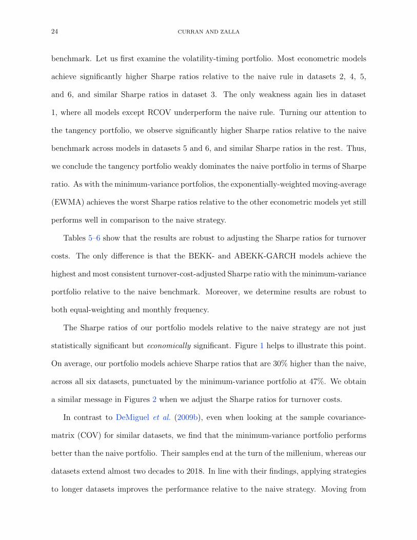
benchmark. Let us first examine the volatility-timing portfolio. Most econometric models
achieve significantly higher Sharpe ratios relative to the naive rule in datasets 2, 4, 5,
and 6, and similar Sharpe ratios in dataset 3. The only weakness again lies in dataset
1, where all models except RCOV underperform the naive rule. Turning our attention to
the tangency portfolio, we observe significantly higher Sharpe ratios relative to the naive
benchmark across models in datasets 5 and 6, and similar Sharpe ratios in the rest. Thus,
we conclude the tangency portfolio weakly dominates the naive portfolio in terms of Sharpe
ratio. As with the minimum-variance portfolios, the exponentially-weighted moving-average
(EWMA) achieves the worst Sharpe ratios relative to the other econometric models yet still
performs well in comparison to the naive strategy.
Tables 5–6 show that the results are robust to adjusting the Sharpe ratios for turnover
costs. The only difference is that the BEKK- and ABEKK-GARCH models achieve the
highest and most consistent turnover-cost-adjusted Sharpe ratio with the minimum-variance
portfolio relative to the naive benchmark. Moreover, we determine results are robust to
both equal-weighting and monthly frequency.
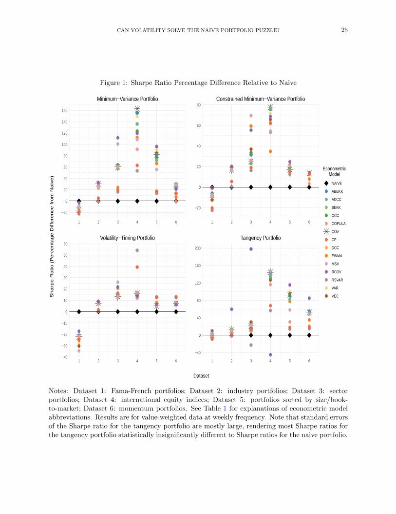
The Sharpe ratios of our portfolio models relative to the naive strategy are not just
statistically significant but economically significant. Figure 1 helps to illustrate this point.
On average, our portfolio models achieve Sharpe ratios that are 30% higher than the naive,
across all six datasets, punctuated by the minimum-variance portfolio at 47%. We obtain
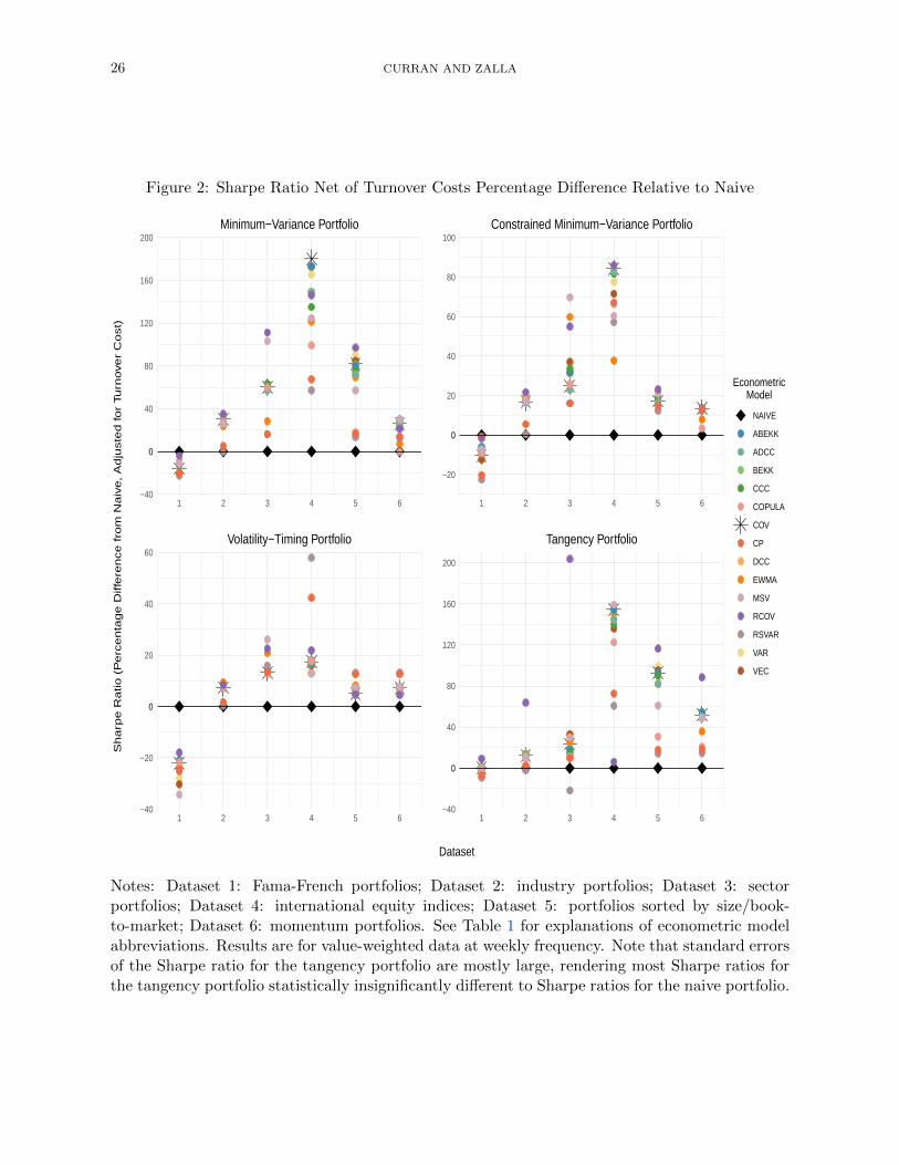
a similar message in Figures 2 when we adjust the Sharpe ratios for turnover costs.
In contrast to DeMiguel et al. (2009b), even when looking at the sample covariance-
matrix (COV) for similar datasets, we find that the minimum-variance portfolio performs
better than the naive portfolio. Their samples end at the turn of the millenium, whereas our
datasets extend almost two decades to 2018. In line with their findings, applying strategies
to longer datasets improves the performance relative to the naive strategy. Moving from
CAN VOLATILITY SOLVE THE NAIVE PORTFOLIO PUZZLE? 25
Figure 1: Sharpe Ratio Percentage Difference Relative to Naive
−20
00
20
40
60
80
100
120
140
160
1 2 3 4 5 6
Minimum−Variance Portfolio
−20
00
20
40
60
80
1 2 3 4 5 6
Constrained Minimum−Variance Portfolio
−40
−30
−20
−10
00
10
20
30
40
50
60
1 2 3 4 5 6
Volatility−Timing Portfolio
−40
00
40
80
120
160
200
1 2 3 4 5 6
Tangency Portfolio
EconometricModel
NAIVE
ABEKK
ADCC
BEKK
CCC
COPULA
COV
CP
DCC
EWMA
MSV
RCOV
RSVAR
VAR
VEC
Dataset
Sh
arp
e R
atio
(P
erc
en
tag
e D
iffe
ren
ce
fro
m N
aiv
e)
Notes: Dataset 1: Fama-French portfolios; Dataset 2: industry portfolios; Dataset 3: sectorportfolios; Dataset 4: international equity indices; Dataset 5: portfolios sorted by size/book-to-market; Dataset 6: momentum portfolios. See Table 1 for explanations of econometric modelabbreviations. Results are for value-weighted data at weekly frequency. Note that standard errorsof the Sharpe ratio for the tangency portfolio are mostly large, rendering most Sharpe ratios forthe tangency portfolio statistically insignificantly different to Sharpe ratios for the naive portfolio.
26 CURRAN AND ZALLA
Figure 2: Sharpe Ratio Net of Turnover Costs Percentage Difference Relative to Naive
−40
00
40
80
120
160
200
1 2 3 4 5 6
Minimum−Variance Portfolio
−20
00
20
40
60
80
100
1 2 3 4 5 6
Constrained Minimum−Variance Portfolio
−40
−20
00
20
40
60
1 2 3 4 5 6
Volatility−Timing Portfolio
−40
00
40
80
120
160
200
1 2 3 4 5 6
Tangency Portfolio
EconometricModel
NAIVE
ABEKK
ADCC
BEKK
CCC
COPULA
COV
CP
DCC
EWMA
MSV
RCOV
RSVAR
VAR
VEC
Dataset
Sh
arp
e R
atio
(P
erc
en
tag
e D
iffe
ren
ce
fro
m N
aiv
e,
Ad
juste
d fo
r Tu
rnove
r C
ost)
Notes: Dataset 1: Fama-French portfolios; Dataset 2: industry portfolios; Dataset 3: sectorportfolios; Dataset 4: international equity indices; Dataset 5: portfolios sorted by size/book-to-market; Dataset 6: momentum portfolios. See Table 1 for explanations of econometric modelabbreviations. Results are for value-weighted data at weekly frequency. Note that standard errorsof the Sharpe ratio for the tangency portfolio are mostly large, rendering most Sharpe ratios forthe tangency portfolio statistically insignificantly different to Sharpe ratios for the naive portfolio.
CAN VOLATILITY SOLVE THE NAIVE PORTFOLIO PUZZLE? 27
monthly to weekly frequency is less important to this result than the period length of the
samples. However, we find that there are econometric models for each portfolio model that
weakly dominate COV in terms of (turnover-cost-adjusted) Sharpe ratios. We also find
in subsection 6.2 that multivariate stochastic volatility (MSV) weakly dominates COV in
terms of portfolio volatility. We thus show that performance improves by employing more
sophisticated econometric models than COV.
6.2 Portfolio Volatility
We next evaluate portfolio volatility. In Tables 7–8, we provide the standard deviations of
the returns associated with each of our thirteen econometric models when used as the input
in each of the four portfolio strategies. We assess portfolio volatility across all six datasets
with value-weighting at weekly frequency. We empirically test the difference in portfolio
volatility between each of the econometric models relative to the naive strategy and report
significance levels.26 The row ordering reflects our attempt to rank the econometric models
according to consistency of performance relative to the naive benchmark.
In the minimum-variance and constrained minimum-variance portfolios, the exponentially-
weighted moving-average (EWMA), realized covariance (RCOV), and multivariate stochas-
tic volatility (MSV) models exhibit significantly lower portfolio volatility relative to the
naive portfolio across all datasets. More importantly, most econometric models strictly
dominate the naive portfolio in terms of volatility performance. The two exceptions, regime-
switching vector autoregression (RSVAR) and combined parameter (CP), which happen to
be the worst ranking models, still weakly dominate the naive benchmark.
For the volatility-timing portfolio, the EWMA model delivers the best results in terms of
portfolio volatility across datasets. Moreover, every econometric model weakly dominates
26Significance corresponds to the Brown-Forsythe F* test for unequal group variances. Results from theDiebold-Mariano (Diebold and Mariano, 1995) test for differences in variance relative to the naive portfolioare similar.
28 CURRAN AND ZALLA
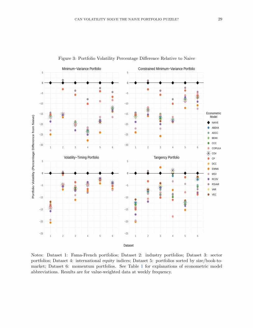
the naive benchmark. For the tangency portfolio, the COPULA achieves the lowest portfolio
volatility across datasets. All econometric models, except RCOV and VEC in dataset
4, weakly dominate the naive benchmark. In addition, the MSV and RCOV models are
consistent runner-ups in both the volatility-timing and tangency portfolio models. Although
the RSVAR and CP models yield the highest volatility, both still weakly dominate the naive
portfolio.
The volatility of our portfolio models relative to the naive strategy is economically
significant. Figure 3 helps to illustrate this point. On average, our portfolio models are 9%
less volatile than the naive, across all six datasets, with the minimum-variance portfolio at
10% lower volatility.
6.3 Portfolio Models
We undertake a holistic evaluation of the econometric models. In Tables 9–12, for each
econometric model, we compare the Sharpe ratio, turnover cost, and portfolio volatility of
each portfolio model across all six datasets. A “✓” indicates that the strategy outperforms
at the 5% significance level or better, a “✓*” indicates a 10% significance level, an “×”
indicates that the strategy underperforms, and a blank space indicates there is no signifi-
cant difference in the strategy’s performance relative to the naive benchmark with respect
to the given performance metric. All of our econometric models are broadly successful at
outperforming the naive portfolio; that is, they achieve higher Sharpe ratios, lower turnover
costs, lower portfolio volatility, or some combination of these superior performance indica-
tors. The few exceptions are concentrated where the volatility-timing portfolio is applied
to dataset 1. In order to aid our identification of the best performers, we develop a simple
heuristic to score individual econometric models: we add up the instances where the model
outperforms the naive benchmark and subtract the instances where the model underper-
CAN VOLATILITY SOLVE THE NAIVE PORTFOLIO PUZZLE? 29
Figure 3: Portfolio Volatility Percentage Difference Relative to Naive
−30
−25
−20
−15
−10
−5
00
5
1 2 3 4 5 6
Minimum−Variance Portfolio
−30
−25
−20
−15
−10
−5
00
5
1 2 3 4 5 6
Constrained Minimum−Variance Portfolio
−25
−20
−15
−10
−5
00
5
1 2 3 4 5 6
Volatility−Timing Portfolio
−25
−20
−15
−10
−5
00
5
1 2 3 4 5 6
Tangency Portfolio
EconometricModel
NAIVE
ABEKK
ADCC
BEKK
CCC
COPULA
COV
CP
DCC
EWMA
MSV
RCOV
RSVAR
VAR
VEC
Dataset
Po
rtfo
lio V
ola
tilit
y (
Pe
rce
nta
ge
Diffe
ren
ce
fro
m N
aiv
e)
Notes: Dataset 1: Fama-French portfolios; Dataset 2: industry portfolios; Dataset 3: sectorportfolios; Dataset 4: international equity indices; Dataset 5: portfolios sorted by size/book-to-market; Dataset 6: momentum portfolios. See Table 1 for explanations of econometric modelabbreviations. Results are for value-weighted data at weekly frequency.

30 CURRAN AND ZALLA
forms.27
The multivariate GARCH models achieve the highest scores relative to other econo-
metric models when applied to the minimum-variance and constrained minimum-variance
strategies. In particular, with GARCH estimates of the covariance matrix, these portfo-
lio strategies weakly dominate the naive benchmark. The constant conditional correlation
(CCC) performs especially well when the no-short-sale constraint is imposed. For the
volatility-timing and tangency portfolios, the realized covariance (RCOV) model exhibits
the most impressive results relative to the naive rule. Specifically, RCOV weakly domi-
nates the naive rule across every dataset when paired with the volatility-timing strategy,
and across five out of six datasets when paired with the tangency portfolio. In general,
our results suggest the multivariate GARCH and RCOV models represent better alterna-
tives to the often-used sample covariance (COV) matrix for portfolio construction. The
sample covariance matrix (COV) performs at the median relative to the other economet-
ric models assessed by our ranking. While the convenience of implementing COV makes
it an attractive option to researchers, our analysis shows there are returns to using more
sophisticated methods to forecast volatility. The worst-ranking econometric models are
the regime-switching vector autoregression (RSVAR) and exponentially-weighted moving-
average (EWMA) models. Nonetheless, both of these models still perform at least as well
as the naive benchmark in every dataset except the Fama-French 3-factor.
As a final assessment, we naively average the estimated conditional volatilities of all
thirteen econometric models to form a combined parameter (CP) model; see Table 12. The
main takeaway from this exercise is that controlling for volatility in a portfolio, no matter
how volatility is estimated, delivers performance metrics that are generally at least as strong
27To clarify, “✓” = 1, “✓*” = 2/3, “ ” (blanks) = 0, and “×” = −1. We discount results that are significantat the 10% level by assigning a value of only 2/3 instead of 1.
CAN VOLATILITY SOLVE THE NAIVE PORTFOLIO PUZZLE? 31
as the naive strategy.
7 Conclusion
We evaluate the out-of-sample performance of mean-variance strategies relying solely upon
the second moment relative to the naive benchmark. Using fourteen econometric models
across six datasets at weekly frequency, we show that the minimum-variance, constrained
minimum-variance, and volatility-timing strategies generally achieve higher Sharpe ratios,
lower turnover costs, and lower portfolio volatility that are economically significant relative
to naive diversification. Whenever mean-variance strategies do not significantly outperform
the naive rule, they usually match and only rarely lose to it.
We identify the econometric models that most consistently and significantly outperform
the 1/N benchmark. First, we show that the multivariate GARCH models weakly dominate
the naive rule when applied to the minimum-variance and constrained minimum-variance
strategies. Next, we demonstrate that the realized covariance model achieves impressive
results when paired with the volatility-timing and tangency portfolios. Even our “worst-
performing” econometric models still manage to perform at least as well as the naive rule in
all but one dataset. Third, we illustrate that if one wishes to prioritize the Sharpe ratio, then
the combined parameter and realized covariance models are excellent choices, even after
controlling for turnover costs. Finally, we show the exponentially-weighted moving-average
and multivariate stochastic volatility models consistently deliver low portfolio volatility.
With the difficulty in consistently outperforming the strategy, the 1/N naive diver-
sification should serve as a benchmark for practitioners and academics. We empirically
demonstrate that one important source of the naive portfolio puzzle is the quality of the
econometric volatility inputs to the mean-variance portfolio strategies. With improved esti-
mates, the mean-variance models can beat the naive portfolio strategy. Our findings imply
32 CURRAN AND ZALLA
that while considerable energy has been devoted to optimizing the mathematical design of
portfolio theory models, more progress may be warranted in improving the estimation of
the moments of asset returns.
References
Adrian, T. and Brunnermeier, M. K. (2016). CoVaR. The American Economic Re-
view, 106 (7), 1705–1741.
Aloui, R., Aıssa, M. S. B. and Nguyen, D. K. (2013). Conditional Dependence Struc-
ture between Oil Prices and Exchange Rates: a Copula-GARCH Approach. Journal of
International Money and Finance, 32 (1), 719–738.
Ao, M., Yingying, L. and Zheng, X. (2019). Approaching Mean-Variance Efficiency for
Large Portfolios. The Review of Financial Studies, 32 (7), 2890–2919.
Baltussen, G. and Post, G. T. (2011). Irrational Diversification: An Examination
of Individual Portfolio Choice. Journal of Financial and Quantitative Analysis, 46 (5),
1463–1491.
Behr, P., Guettler, A. and Miebs, F. (2013). On Portfolio Optimization: Imposing
the Right Constraints. Journal of Banking & Finance, 37 (4), 1232–1242.
Bekiros, S., Boubaker, S., Nguyen, D. K. and Uddin, G. S. (2017). Black Swan
Events and Safe Havens: The Role of Gold in Globally Integrated Emerging Markets.
Journal of International Money and Finance, 73, 317 – 334.
Benartzi, S. and Thaler, R. H. (2001). Naive Diversification Strategies in Defined
Contribution Saving Plans. American Economic Review, 91 (1), 79–98.
CAN VOLATILITY SOLVE THE NAIVE PORTFOLIO PUZZLE? 33
Bodnar, T. and Hautsch, N. (2016). Dynamic Conditional Correlation Multiplicative
Error Processes. Journal of Empirical Finance, 36, 41 – 67.
Bollerslev, T. et al. (1990). Modelling the Coherence in Short-Run Nominal Exchange
Rates: a Multivariate Generalized ARCH Model. The Review of Economics and Statis-
tics, 72 (3), 498–505.
Brandt, M. W., Santa-Clara, P. and Valkanov, R. (2009). Parametric Portfolio
Policies: Exploiting Characteristics in the Cross-Section of Equity Returns. The Review
of Financial Studies, 22 (9), 3411–3447.
Cappiello, L., Engle, R. F. and Sheppard, K. (2006). Asymmetric Dynamics in the
Correlations of Global Equity and Bond Returns. Journal of Financial Econometrics,
4 (4), 537–572.
Chan, J. C. and Eisenstat, E. (2018). Bayesian Model Comparison for Time-Varying
Parameter VARs with Stochastic Volatility. Journal of Applied Econometrics, 33 (4),
509–532.
Chopra, V. K. and Ziemba, W. T. (2013). The Effect of Errors in Means, Variances, and
Covariances on Optimal Portfolio Choice. In Handbook of the Fundamentals of Financial
Decision Making: Part I, World Scientific, pp. 365–373.
Christoffersen, P., Errunza, V., Jacobs, K. and Langlois, H. (2012). Is the
Potential for International Diversification Disappearing? A Dynamic Copula Approach.
The Review of Financial Studies, 25 (12), 3711–3751.
— and Langlois, H. (2013). The Joint Dynamics of Equity Market Factors. The Journal
of Financial and Quantitative Analysis, 48 (5), 1371–1404.
34 CURRAN AND ZALLA
Creal, D., Koopman, S. J. and Lucas, A. (2013). Generalized Autoregressive Score
Models with Applications. Journal of Applied Econometrics, 28 (5), 777–795.
De Giorgi, E. G. and Mahmoud, O. (2018). Naive Diversification Preferences and
Their Representation. Working paper.
DeMiguel, V., Garlappi, L., Nogales, F. J. and Uppal, R. (2009a). A Generalized
Approach to Portfolio Optimization: Improving Performance by Constraining Portfolio
Norms. Management Science, 55 (5), 798–812.
—, — and Uppal, R. (2009b). Optimal Versus Naive Diversification: How Inefficient is
the 1/N Portfolio Strategy? The Review of Financial Studies, 22 (5), 1915–1953.
—, Nogales, F. J. and Uppal, R. (2014). Stock Return Serial Dependence and Out-of-
Sample Portfolio Performance. The Review of Financial Studies, 27 (4), 1031–1073.
—, Plyakha, Y., Uppal, R. and Vilkov, G. (2013). Improving Portfolio Selection Using
Option-Implied Volatility and Skewness. Journal of Financial and Quantitative Analysis,
48 (6), 1813–1845.
Diebold, F. X. and Mariano, R. S. (1995). Comparing Predictive Accuracy. Journal
of Business & Economic Statistics, 13 (3), 253–263.
Duchin, R. and Levy, H. (2009). Markowitz Versus the Talmudic Portfolio Diversification
Strategies. The Journal of Portfolio Management, 35, 71–74.
Engle, R. (2002). Dynamic Conditional Correlation: A Simple Class of Multivariate
Generalized Autoregressive Conditional Heteroskedasticity Models. Journal of Business
& Economic Statistics, 20 (3), 339–350.
CAN VOLATILITY SOLVE THE NAIVE PORTFOLIO PUZZLE? 35
Engle, R. F. and Kroner, K. F. (1995). Multivariate Simultaneous Generalized ARCH.
Econometric Theory, 11 (1), 122–150.
Fletcher, J. (2011). Do Optimal Diversification Strategies Outperform the 1/N Strategy
in UK Stock Returns? International Review of Financial Analysis, 20 (5), 375–385.
Gathergood, J., Hirshleifer, D., Leake, D., Sakaguchi, H. and Stewart, N.
(2019). Naıve *Buying* Diversification and Narrow Framing by Individual Investors.
Working Paper 25567, NBER.
Higham, N. J. (1990). Analysis of the Cholesky Decomposition of a Semi-Definite Matrix.
Oxford University Press.
Jagannathan, R. and Ma, T. (2003). Risk Reduction in Large Portfolios: Why Imposing
the Wrong Constraints Helps. The Journal of Finance, 58 (4), 1651–1683.
Jobson, J. D. and Korkie, B. (1980). Estimation for Markowitz Efficient Portfolios.
Journal of the American Statistical Association, 75 (371), 544–554.
Johansen, S. (1988). Statistical Analysis of Cointegration Vectors. Journal of Economic
Dynamics and Control, 12 (2-3), 231–254.
— (1991). Estimation and Hypothesis Testing of Cointegration Vectors in Gaussian Vector
Autoregressive Models. Econometrica, pp. 1551–1580.
Kastner, G. (2019a). factorstochvol: Bayesian Estimation of (Sparse) Latent Factor
Stochastic Volatility Models. R package version 0.9.2.
— (2019b). Sparse Bayesian Time-Varying Covariance Estimation in Many Dimensions.
Journal of Econometrics, 210 (1), 98–115.
36 CURRAN AND ZALLA
Kirby, C. and Ostdiek, B. (2012). It’s All in the Timing: Simple Active Portfolio
Strategies that Outperform Naive Diversification. Journal of Financial and Quantitative
Analysis, 47 (2), 437–467.
Kourtis, A., Dotsis, G. and Markellos, R. N. (2012). Parameter Uncertainty in
Portfolio Selection: Shrinking the Inverse Covariance Matrix. Journal of Banking & Fi-
nance, 36 (9), 2522–2531.
Ledoit, O. and Wolf, M. (2003). Improved Estimation of the Covariance Matrix of
Stock Returns with an Application to Portfolio Selection. Journal of Empirical Finance,
10 (5), 603–621.
— and — (2008). Robust Performance Hypothesis Testing with the Sharpe Ratio. Journal
of Empirical Finance, 15 (5), 850–859.
— and — (2017). Nonlinear Shrinkage of the Covariance Matrix for Portfolio Selection:
Markowitz Meets Goldilocks. The Review of Financial Studies, 30 (12), 4349–4388.
Markowitz, H. (1952). Portfolio Selection. The Journal of Finance, 7 (1), 77–91.
Merton, R. C. (1980). On Estimating the Expected Return on the Market: An Ex-
ploratory Investigation. Journal of Financial Economics, 8 (4), 323–361.
Michaud, R. O. and Michaud, R. O. (2008). Efficient Asset Management: A Practical
Guide to Stock Portfolio Optimization and Asset Allocation. Oxford University Press,
2nd edn.
Moreira, A. and Muir, T. (2017). Volatility-Managed Portfolios. The Journal of Fi-
nance, 72 (4), 1611–1644.
CAN VOLATILITY SOLVE THE NAIVE PORTFOLIO PUZZLE? 37
— and — (2019). Should Long-Term Investors Time Volatility? Journal of Financial
Economics, 131 (3), 507–527.
Pflug, G. C., Pichler, A. and Wozabal, D. (2012). The 1/N Investment Strategy is
Optimal Under High Model Ambiguity. Journal of Banking & Finance, 36 (2), 410–417.
Sklar, M. (1959). Fonctions de Repartition an Dimensions et Leurs Marges. Publ. Inst.
Statist. Univ. Paris, 8, 229–231.
Solnik, B. and Watewai, T. (2016). International Correlation Asymmetries: Frequent-
but-Small and Infrequent-but-Large Equity Returns. Review of Asset Pricing Studies,
6 (2), 221 – 260.
Stock, J. H. and Watson, M. W. (2003). Forecasting Output and Inflation: The Role
of Asset Prices. Journal of Economic Literature, 41 (3), 788–829.
— and — (2004). Combination Forecasts of Output Growth in a Seven-Country Data Set.
Journal of Forecasting, 23 (6), 405–430.
Stric, C. and Granger, C. (2005). Nonstationarities in Stock Returns. The Review of
Economics and Statistics, 87 (3), 503–522.
Trucıos, C., Zevallos, M., Hotta, L. K. and Santos, A. A. (2019). Covariance
Prediction in Large Portfolio Allocation. Econometrica, 7 (2), 19.
Tu, J. and Zhou, G. (2011). Markowitz Meets Talmud: A Combination of Sophisticated
and Naive Diversification Strategies. Journal of Financial Economics, 99 (1), 204–215.
Vogiatzoglou, M. (2017). Dynamic Copula Toolbox. Available at SSRN 2956888.

38 CURRAN AND ZALLA
Wang, Y., Wu, C. and Yang, L. (2015). Hedging with Futures: Does Anything Beat
the Naıve Hedging Strategy? Management Science, 61 (12), 2870–2889.
Xiao, Z. (2014). Right-Tail Information in Financial Markets. Econometric Theory, 30 (1),
94–126.
Zimmer, D. M. (2012). The Role of Copulas in the Housing Crisis. The Review of Eco-
nomics and Statistics, 94 (2), 607–620.
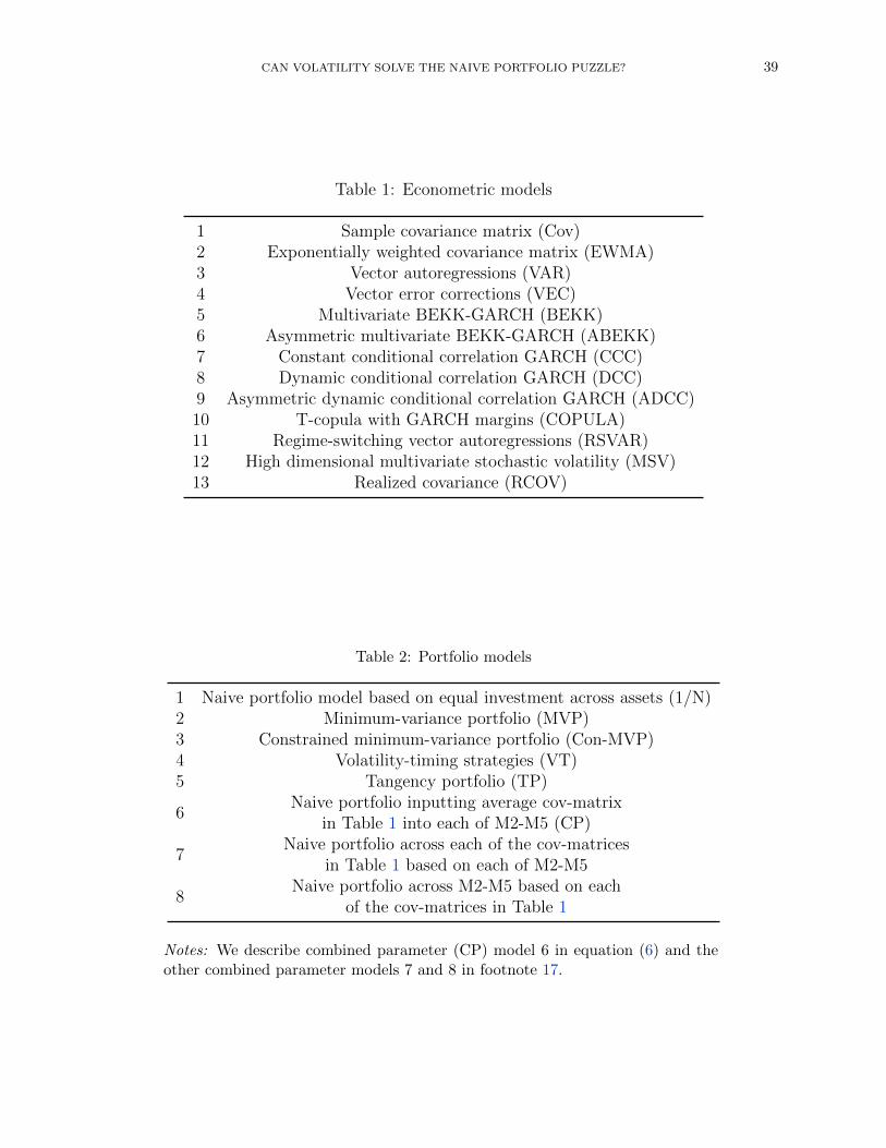
CAN VOLATILITY SOLVE THE NAIVE PORTFOLIO PUZZLE? 39
Table 1: Econometric models
1 Sample covariance matrix (Cov)2 Exponentially weighted covariance matrix (EWMA)3 Vector autoregressions (VAR)4 Vector error corrections (VEC)5 Multivariate BEKK-GARCH (BEKK)6 Asymmetric multivariate BEKK-GARCH (ABEKK)7 Constant conditional correlation GARCH (CCC)8 Dynamic conditional correlation GARCH (DCC)9 Asymmetric dynamic conditional correlation GARCH (ADCC)10 T-copula with GARCH margins (COPULA)11 Regime-switching vector autoregressions (RSVAR)12 High dimensional multivariate stochastic volatility (MSV)13 Realized covariance (RCOV)
Table 2: Portfolio models
1 Naive portfolio model based on equal investment across assets (1/N)2 Minimum-variance portfolio (MVP)3 Constrained minimum-variance portfolio (Con-MVP)4 Volatility-timing strategies (VT)5 Tangency portfolio (TP)
6Naive portfolio inputting average cov-matrix
in Table 1 into each of M2-M5 (CP)
7Naive portfolio across each of the cov-matrices
in Table 1 based on each of M2-M5
8Naive portfolio across M2-M5 based on each
of the cov-matrices in Table 1
Notes: We describe combined parameter (CP) model 6 in equation (6) and theother combined parameter models 7 and 8 in footnote 17.
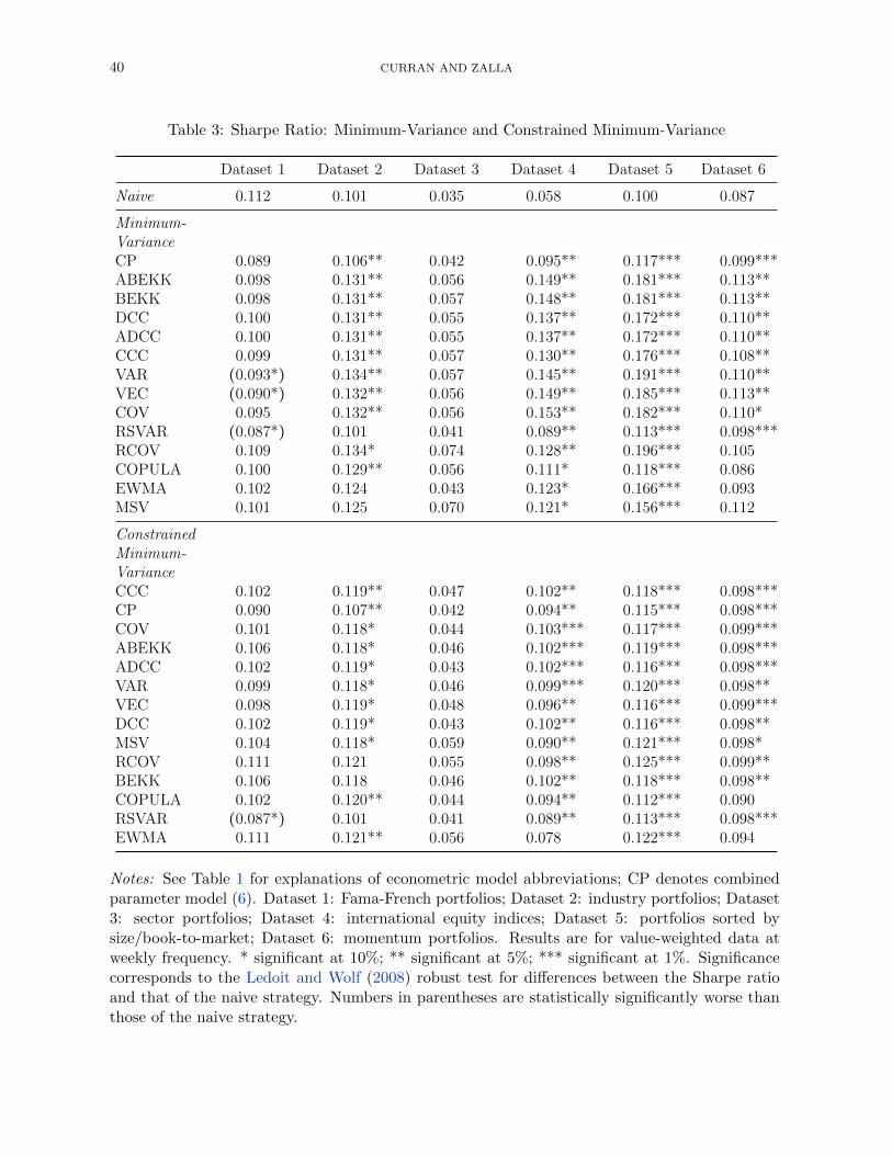
40 CURRAN AND ZALLA
Table 3: Sharpe Ratio: Minimum-Variance and Constrained Minimum-Variance
Dataset 1 Dataset 2 Dataset 3 Dataset 4 Dataset 5 Dataset 6
Naive 0.112 0.101 0.035 0.058 0.100 0.087
Minimum-VarianceCP 0.089 0.106** 0.042 0.095** 0.117*** 0.099***ABEKK 0.098 0.131** 0.056 0.149** 0.181*** 0.113**BEKK 0.098 0.131** 0.057 0.148** 0.181*** 0.113**DCC 0.100 0.131** 0.055 0.137** 0.172*** 0.110**ADCC 0.100 0.131** 0.055 0.137** 0.172*** 0.110**CCC 0.099 0.131** 0.057 0.130** 0.176*** 0.108**VAR (0.093*) 0.134** 0.057 0.145** 0.191*** 0.110**VEC (0.090*) 0.132** 0.056 0.149** 0.185*** 0.113**COV 0.095 0.132** 0.056 0.153** 0.182*** 0.110*RSVAR (0.087*) 0.101 0.041 0.089** 0.113*** 0.098***RCOV 0.109 0.134* 0.074 0.128** 0.196*** 0.105COPULA 0.100 0.129** 0.056 0.111* 0.118*** 0.086EWMA 0.102 0.124 0.043 0.123* 0.166*** 0.093MSV 0.101 0.125 0.070 0.121* 0.156*** 0.112
ConstrainedMinimum-VarianceCCC 0.102 0.119** 0.047 0.102** 0.118*** 0.098***CP 0.090 0.107** 0.042 0.094** 0.115*** 0.098***COV 0.101 0.118* 0.044 0.103*** 0.117*** 0.099***ABEKK 0.106 0.118* 0.046 0.102*** 0.119*** 0.098***ADCC 0.102 0.119* 0.043 0.102*** 0.116*** 0.098***VAR 0.099 0.118* 0.046 0.099*** 0.120*** 0.098**VEC 0.098 0.119* 0.048 0.096** 0.116*** 0.099***DCC 0.102 0.119* 0.043 0.102** 0.116*** 0.098**MSV 0.104 0.118* 0.059 0.090** 0.121*** 0.098*RCOV 0.111 0.121 0.055 0.098** 0.125*** 0.099**BEKK 0.106 0.118 0.046 0.102** 0.118*** 0.098**COPULA 0.102 0.120** 0.044 0.094** 0.112*** 0.090RSVAR (0.087*) 0.101 0.041 0.089** 0.113*** 0.098***EWMA 0.111 0.121** 0.056 0.078 0.122*** 0.094
Notes: See Table 1 for explanations of econometric model abbreviations; CP denotes combinedparameter model (6). Dataset 1: Fama-French portfolios; Dataset 2: industry portfolios; Dataset3: sector portfolios; Dataset 4: international equity indices; Dataset 5: portfolios sorted bysize/book-to-market; Dataset 6: momentum portfolios. Results are for value-weighted data atweekly frequency. * significant at 10%; ** significant at 5%; *** significant at 1%. Significancecorresponds to the Ledoit and Wolf (2008) robust test for differences between the Sharpe ratioand that of the naive strategy. Numbers in parentheses are statistically significantly worse thanthose of the naive strategy.
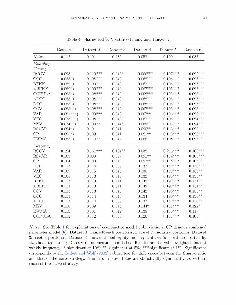
CAN VOLATILITY SOLVE THE NAIVE PORTFOLIO PUZZLE? 41
Table 4: Sharpe Ratio: Volatility-Timing and Tangency
Dataset 1 Dataset 2 Dataset 3 Dataset 4 Dataset 5 Dataset 6
Naive 0.112 0.101 0.035 0.058 0.100 0.087
VolatilityTimingRCOV 0.093 0.110*** 0.043* 0.066*** 0.107*** 0.092***CCC (0.088*) 0.108*** 0.040 0.068*** 0.106*** 0.093***BEKK (0.089*) 0.109*** 0.040 0.067*** 0.105*** 0.093***ABEKK (0.089*) 0.109*** 0.040 0.067*** 0.105*** 0.093***COPULA (0.088*) 0.108*** 0.040 0.068*** 0.105*** 0.093***ADCC (0.088*) 0.108*** 0.040 0.068*** 0.105*** 0.093***DCC (0.088*) 0.108** 0.040 0.068*** 0.105*** 0.093***COV (0.088**) 0.108*** 0.040 0.067*** 0.105*** 0.093***VAR (0.081***) 0.109*** 0.040 0.067** 0.106*** 0.093***VEC (0.078***) 0.108** 0.040 0.067*** 0.105*** 0.094***MSV (0.074**) 0.109** 0.044* 0.065* 0.107*** 0.094**RSVAR (0.084*) 0.101 0.041 0.090** 0.113*** 0.098***CP (0.085*) 0.103 0.041 0.081** 0.113*** 0.098***EWMA (0.085*) 0.110** 0.042 0.065 0.108*** 0.093**
TangencyRCOV 0.124 0.161*** 0.104** 0.032 0.215*** 0.160***RSVAR 0.102 0.099 0.027 0.091** 0.114*** 0.100***CP 0.104 0.103 0.040 0.097** 0.118*** 0.103**DCC 0.113 0.114 0.038 0.137 0.182*** 0.130***VAR 0.109 0.115 0.045 0.135 0.199*** 0.133**VEC 0.108 0.113 0.046 0.132 0.195*** 0.135**BEKK 0.113 0.113 0.041 0.142 0.192*** 0.134**ABEKK 0.113 0.113 0.041 0.142 0.192*** 0.134**COV 0.113 0.113 0.043 0.142 0.193*** 0.133**CCC 0.113 0.114 0.040 0.134 0.190*** 0.130**ADCC 0.113 0.114 0.038 0.137 0.182*** 0.130**MSV 0.110 0.109 0.043 0.144* 0.158*** 0.128*EWMA 0.112 0.101 0.042 0.138 0.178*** 0.117COPULA 0.112 0.112 0.038 0.126 0.131*** 0.105
Notes: See Table 1 for explanations of econometric model abbreviations; CP denotes combinedparameter model (6). Dataset 1: Fama-French portfolios; Dataset 2: industry portfolios; Dataset3: sector portfolios; Dataset 4: international equity indices; Dataset 5: portfolios sorted bysize/book-to-market; Dataset 6: momentum portfolios. Results are for value-weighted data atweekly frequency. * significant at 10%; ** significant at 5%; *** significant at 1%. Significancecorresponds to the Ledoit and Wolf (2008) robust test for differences between the Sharpe ratioand that of the naive strategy. Numbers in parentheses are statistically significantly worse thanthose of the naive strategy.
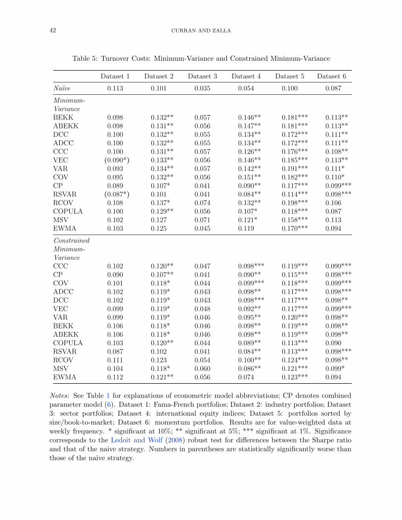
42 CURRAN AND ZALLA
Table 5: Turnover Costs: Minimum-Variance and Constrained Minimum-Variance
Dataset 1 Dataset 2 Dataset 3 Dataset 4 Dataset 5 Dataset 6
Naıve 0.113 0.101 0.035 0.054 0.100 0.087
Minimum-VarianceBEKK 0.098 0.132** 0.057 0.146** 0.181*** 0.113**ABEKK 0.098 0.131** 0.056 0.147** 0.181*** 0.113**DCC 0.100 0.132** 0.055 0.134** 0.172*** 0.111**ADCC 0.100 0.132** 0.055 0.134** 0.172*** 0.111**CCC 0.100 0.131** 0.057 0.126** 0.176*** 0.108**VEC (0.090*) 0.133** 0.056 0.146** 0.185*** 0.113**VAR 0.093 0.134** 0.057 0.142** 0.191*** 0.111*COV 0.095 0.132** 0.056 0.151** 0.182*** 0.110*CP 0.089 0.107* 0.041 0.090** 0.117*** 0.099***RSVAR (0.087*) 0.101 0.041 0.084** 0.114*** 0.098***RCOV 0.108 0.137* 0.074 0.132** 0.198*** 0.106COPULA 0.100 0.129** 0.056 0.107* 0.118*** 0.087MSV 0.102 0.127 0.071 0.121* 0.158*** 0.113EWMA 0.103 0.125 0.045 0.119 0.170*** 0.094
ConstrainedMinimum-VarianceCCC 0.102 0.120** 0.047 0.098*** 0.119*** 0.099***CP 0.090 0.107** 0.041 0.090** 0.115*** 0.098***COV 0.101 0.118* 0.044 0.099*** 0.118*** 0.099***ADCC 0.102 0.119* 0.043 0.098** 0.117*** 0.098***DCC 0.102 0.119* 0.043 0.098*** 0.117*** 0.098**VEC 0.099 0.119* 0.048 0.092** 0.117*** 0.099***VAR 0.099 0.119* 0.046 0.095** 0.120*** 0.098**BEKK 0.106 0.118* 0.046 0.098** 0.119*** 0.098**ABEKK 0.106 0.118* 0.046 0.098** 0.119*** 0.098**COPULA 0.103 0.120** 0.044 0.089** 0.113*** 0.090RSVAR 0.087 0.102 0.041 0.084** 0.113*** 0.098***RCOV 0.111 0.123 0.054 0.100** 0.124*** 0.098**MSV 0.104 0.118* 0.060 0.086** 0.121*** 0.099*EWMA 0.112 0.121** 0.056 0.074 0.123*** 0.094
Notes: See Table 1 for explanations of econometric model abbreviations; CP denotes combinedparameter model (6). Dataset 1: Fama-French portfolios; Dataset 2: industry portfolios; Dataset3: sector portfolios; Dataset 4: international equity indices; Dataset 5: portfolios sorted bysize/book-to-market; Dataset 6: momentum portfolios. Results are for value-weighted data atweekly frequency. * significant at 10%; ** significant at 5%; *** significant at 1%. Significancecorresponds to the Ledoit and Wolf (2008) robust test for differences between the Sharpe ratioand that of the naive strategy. Numbers in parentheses are statistically significantly worse thanthose of the naive strategy.
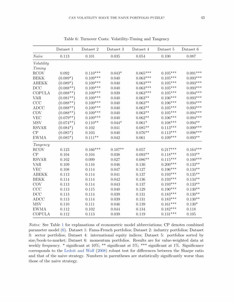
CAN VOLATILITY SOLVE THE NAIVE PORTFOLIO PUZZLE? 43
Table 6: Turnover Costs: Volatility-Timing and Tangency
Dataset 1 Dataset 2 Dataset 3 Dataset 4 Dataset 5 Dataset 6
Naıve 0.113 0.101 0.035 0.054 0.100 0.087
VolatilityTimingRCOV 0.092 0.110*** 0.043* 0.065*** 0.105*** 0.091***BEKK (0.089*) 0.109*** 0.040 0.063*** 0.105*** 0.093***ABEKK (0.089*) 0.109*** 0.040 0.063*** 0.105*** 0.093***DCC (0.088**) 0.109*** 0.040 0.063*** 0.105*** 0.093***COPULA (0.088**) 0.109*** 0.039 0.063*** 0.105*** 0.094***VAR (0.081**) 0.109*** 0.040 0.063** 0.106*** 0.093***CCC (0.088**) 0.109*** 0.040 0.063** 0.106*** 0.094***ADCC (0.088**) 0.109*** 0.040 0.063** 0.105*** 0.093***COV (0.088**) 0.109*** 0.040 0.063** 0.105*** 0.094***VEC (0.079**) 0.109*** 0.040 0.062** 0.106*** 0.094***MSV (0.074**) 0.110** 0.044* 0.061* 0.108*** 0.094**RSVAR (0.084*) 0.102 0.041 0.085** 0.113*** 0.099***CP (0.085*) 0.103 0.040 0.076** 0.113*** 0.098***EWMA (0.085*) 0.111** 0.042 0.061 0.109*** 0.093**
TangencyRCOV 0.123 0.166*** 0.107** 0.057 0.217*** 0.164***CP 0.104 0.104 0.038 0.093** 0.118*** 0.103**RSVAR 0.102 0.099 0.027 0.086** 0.115*** 0.100***VAR 0.109 0.116 0.046 0.130 0.200*** 0.133**VEC 0.108 0.114 0.047 0.127 0.196*** 0.134**ABEKK 0.113 0.114 0.041 0.137 0.193*** 0.135**BEKK 0.114 0.114 0.042 0.136 0.193*** 0.134**COV 0.113 0.114 0.043 0.137 0.193*** 0.133**CCC 0.113 0.115 0.040 0.129 0.190*** 0.130**DCC 0.113 0.114 0.039 0.131 0.183*** 0.130**ADCC 0.113 0.114 0.039 0.131 0.183*** 0.130**MSV 0.110 0.111 0.046 0.139 0.161*** 0.130*EWMA 0.112 0.102 0.044 0.134 0.182*** 0.118COPULA 0.112 0.113 0.039 0.119 0.131*** 0.105
Notes: See Table 1 for explanations of econometric model abbreviations; CP denotes combinedparameter model (6). Dataset 1: Fama-French portfolios; Dataset 2: industry portfolios; Dataset3: sector portfolios; Dataset 4: international equity indices; Dataset 5: portfolios sorted bysize/book-to-market; Dataset 6: momentum portfolios. Results are for value-weighted data atweekly frequency. * significant at 10%; ** significant at 5%; *** significant at 1%. Significancecorresponds to the Ledoit and Wolf (2008) robust test for differences between the Sharpe ratioand that of the naive strategy. Numbers in parentheses are statistically significantly worse thanthose of the naive strategy.
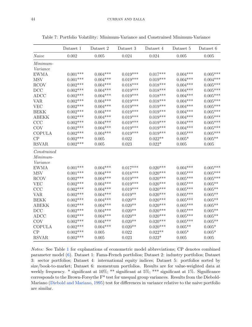
44 CURRAN AND ZALLA
Table 7: Portfolio Volatility: Minimum-Variance and Constrained Minimum-Variance
Dataset 1 Dataset 2 Dataset 3 Dataset 4 Dataset 5 Dataset 6
Naive 0.002 0.005 0.024 0.024 0.005 0.005
Minimum-VarianceEWMA 0.001*** 0.004*** 0.019*** 0.017*** 0.004*** 0.005***MSV 0.001*** 0.004*** 0.019*** 0.019*** 0.004*** 0.004***RCOV 0.002*** 0.004*** 0.018*** 0.018*** 0.004*** 0.005***DCC 0.002*** 0.004*** 0.019*** 0.018*** 0.004*** 0.005***ADCC 0.002*** 0.004*** 0.019*** 0.018*** 0.004*** 0.005***VAR 0.002*** 0.004*** 0.019*** 0.018*** 0.004*** 0.005***VEC 0.002*** 0.004*** 0.019*** 0.019*** 0.004*** 0.005***BEKK 0.002*** 0.004*** 0.019*** 0.019*** 0.004*** 0.005***ABEKK 0.002*** 0.004*** 0.019*** 0.019*** 0.004*** 0.005***CCC 0.002*** 0.004*** 0.019*** 0.019*** 0.004*** 0.005***COV 0.002*** 0.004*** 0.019*** 0.019*** 0.004*** 0.005***COPULA 0.002*** 0.004*** 0.019*** 0.019*** 0.005*** 0.005***CP 0.002*** 0.005 0.022 0.022** 0.005* 0.005**RSVAR 0.002*** 0.005 0.023 0.022* 0.005 0.005
ConstrainedMinimum-VarianceEWMA 0.001*** 0.004*** 0.017*** 0.020*** 0.004*** 0.005***MSV 0.001*** 0.004*** 0.018*** 0.020*** 0.005*** 0.005***RCOV 0.002*** 0.004*** 0.019*** 0.020*** 0.005*** 0.005***VEC 0.002*** 0.004*** 0.019*** 0.020*** 0.005*** 0.005**CCC 0.002*** 0.004*** 0.019*** 0.020*** 0.005*** 0.005**VAR 0.002*** 0.004*** 0.019** 0.020*** 0.005*** 0.005**BEKK 0.002*** 0.004*** 0.020** 0.020*** 0.005*** 0.005**ABEKK 0.002*** 0.004*** 0.020** 0.020*** 0.005*** 0.005**DCC 0.002*** 0.004*** 0.020** 0.020*** 0.005*** 0.005**ADCC 0.002*** 0.004*** 0.020** 0.020*** 0.005*** 0.005**COV 0.002*** 0.004*** 0.020** 0.020*** 0.005*** 0.005**COPULA 0.002*** 0.004*** 0.020** 0.020*** 0.005** 0.005*CP 0.002*** 0.005 0.022 0.022** 0.005* 0.005*RSVAR 0.002*** 0.005 0.023 0.022* 0.005 0.005
Notes: See Table 1 for explanations of econometric model abbreviations; CP denotes combinedparameter model (6). Dataset 1: Fama-French portfolios; Dataset 2: industry portfolios; Dataset3: sector portfolios; Dataset 4: international equity indices; Dataset 5: portfolios sorted bysize/book-to-market; Dataset 6: momentum portfolios. Results are for value-weighted data atweekly frequency. * significant at 10%; ** significant at 5%; *** significant at 1%. Significancecorresponds to the Brown-Forsythe F* test for unequal group variances. Results from the Diebold-Mariano (Diebold and Mariano, 1995) test for differences in variance relative to the naive portfolioare similar.
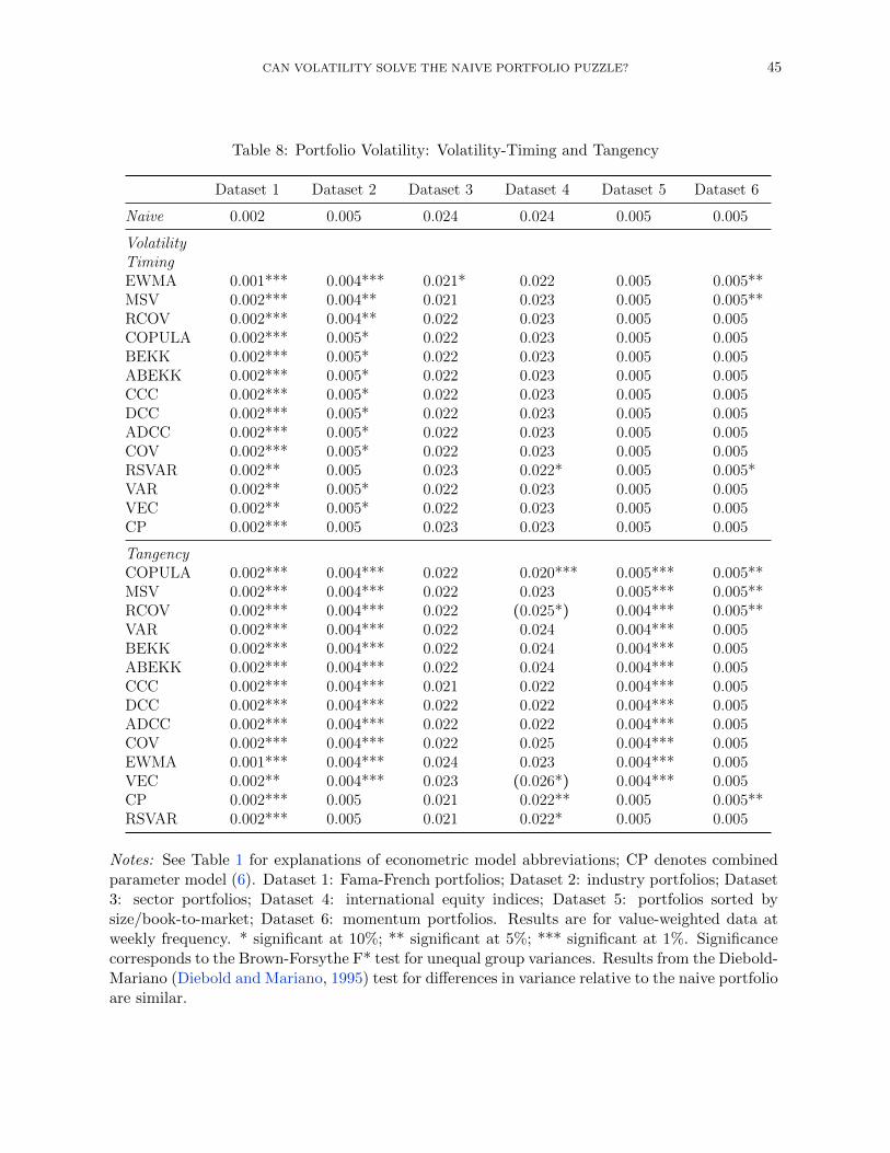
CAN VOLATILITY SOLVE THE NAIVE PORTFOLIO PUZZLE? 45
Table 8: Portfolio Volatility: Volatility-Timing and Tangency
Dataset 1 Dataset 2 Dataset 3 Dataset 4 Dataset 5 Dataset 6
Naive 0.002 0.005 0.024 0.024 0.005 0.005
VolatilityTimingEWMA 0.001*** 0.004*** 0.021* 0.022 0.005 0.005**MSV 0.002*** 0.004** 0.021 0.023 0.005 0.005**RCOV 0.002*** 0.004** 0.022 0.023 0.005 0.005COPULA 0.002*** 0.005* 0.022 0.023 0.005 0.005BEKK 0.002*** 0.005* 0.022 0.023 0.005 0.005ABEKK 0.002*** 0.005* 0.022 0.023 0.005 0.005CCC 0.002*** 0.005* 0.022 0.023 0.005 0.005DCC 0.002*** 0.005* 0.022 0.023 0.005 0.005ADCC 0.002*** 0.005* 0.022 0.023 0.005 0.005COV 0.002*** 0.005* 0.022 0.023 0.005 0.005RSVAR 0.002** 0.005 0.023 0.022* 0.005 0.005*VAR 0.002** 0.005* 0.022 0.023 0.005 0.005VEC 0.002** 0.005* 0.022 0.023 0.005 0.005CP 0.002*** 0.005 0.023 0.023 0.005 0.005
TangencyCOPULA 0.002*** 0.004*** 0.022 0.020*** 0.005*** 0.005**MSV 0.002*** 0.004*** 0.022 0.023 0.005*** 0.005**RCOV 0.002*** 0.004*** 0.022 (0.025*) 0.004*** 0.005**VAR 0.002*** 0.004*** 0.022 0.024 0.004*** 0.005BEKK 0.002*** 0.004*** 0.022 0.024 0.004*** 0.005ABEKK 0.002*** 0.004*** 0.022 0.024 0.004*** 0.005CCC 0.002*** 0.004*** 0.021 0.022 0.004*** 0.005DCC 0.002*** 0.004*** 0.022 0.022 0.004*** 0.005ADCC 0.002*** 0.004*** 0.022 0.022 0.004*** 0.005COV 0.002*** 0.004*** 0.022 0.025 0.004*** 0.005EWMA 0.001*** 0.004*** 0.024 0.023 0.004*** 0.005VEC 0.002** 0.004*** 0.023 (0.026*) 0.004*** 0.005CP 0.002*** 0.005 0.021 0.022** 0.005 0.005**RSVAR 0.002*** 0.005 0.021 0.022* 0.005 0.005
Notes: See Table 1 for explanations of econometric model abbreviations; CP denotes combinedparameter model (6). Dataset 1: Fama-French portfolios; Dataset 2: industry portfolios; Dataset3: sector portfolios; Dataset 4: international equity indices; Dataset 5: portfolios sorted bysize/book-to-market; Dataset 6: momentum portfolios. Results are for value-weighted data atweekly frequency. * significant at 10%; ** significant at 5%; *** significant at 1%. Significancecorresponds to the Brown-Forsythe F* test for unequal group variances. Results from the Diebold-Mariano (Diebold and Mariano, 1995) test for differences in variance relative to the naive portfolioare similar.
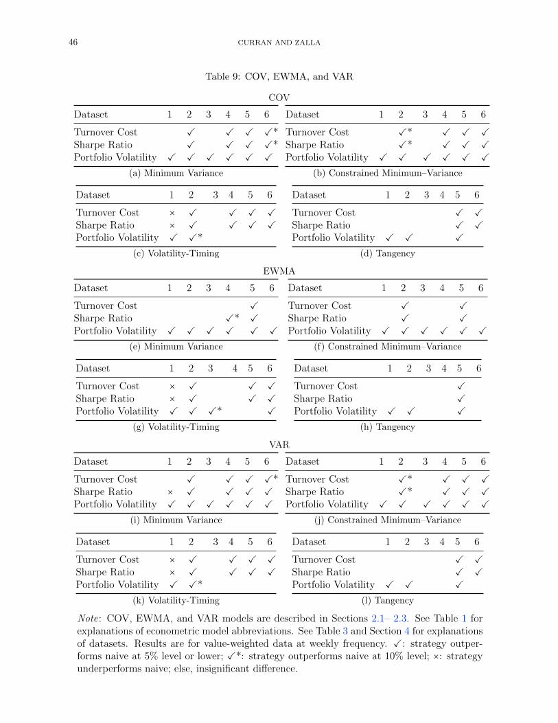
46 CURRAN AND ZALLA
Table 9: COV, EWMA, and VAR
COV
Dataset 1 2 3 4 5 6
Turnover Cost ✓ ✓ ✓ ✓*Sharpe Ratio ✓ ✓ ✓ ✓*Portfolio Volatility ✓ ✓ ✓ ✓ ✓ ✓
(a) Minimum Variance
Dataset 1 2 3 4 5 6
Turnover Cost ✓* ✓ ✓ ✓Sharpe Ratio ✓* ✓ ✓ ✓Portfolio Volatility ✓ ✓ ✓ ✓ ✓ ✓
(b) Constrained Minimum–Variance
Dataset 1 2 3 4 5 6
Turnover Cost × ✓ ✓ ✓ ✓Sharpe Ratio × ✓ ✓ ✓ ✓Portfolio Volatility ✓ ✓*
(c) Volatility-Timing
Dataset 1 2 3 4 5 6
Turnover Cost ✓ ✓Sharpe Ratio ✓ ✓Portfolio Volatility ✓ ✓ ✓
(d) Tangency
EWMA
Dataset 1 2 3 4 5 6
Turnover Cost ✓Sharpe Ratio ✓* ✓Portfolio Volatility ✓ ✓ ✓ ✓ ✓ ✓
(e) Minimum Variance
Dataset 1 2 3 4 5 6
Turnover Cost ✓ ✓Sharpe Ratio ✓ ✓Portfolio Volatility ✓ ✓ ✓ ✓ ✓ ✓
(f) Constrained Minimum–Variance
Dataset 1 2 3 4 5 6
Turnover Cost × ✓ ✓ ✓Sharpe Ratio × ✓ ✓ ✓Portfolio Volatility ✓ ✓ ✓* ✓
(g) Volatility-Timing
Dataset 1 2 3 4 5 6
Turnover Cost ✓Sharpe Ratio ✓Portfolio Volatility ✓ ✓ ✓
(h) Tangency
VAR
Dataset 1 2 3 4 5 6
Turnover Cost ✓ ✓ ✓ ✓*Sharpe Ratio × ✓ ✓ ✓ ✓Portfolio Volatility ✓ ✓ ✓ ✓ ✓ ✓
(i) Minimum Variance
Dataset 1 2 3 4 5 6
Turnover Cost ✓* ✓ ✓ ✓Sharpe Ratio ✓* ✓ ✓ ✓Portfolio Volatility ✓ ✓ ✓ ✓ ✓ ✓
(j) Constrained Minimum–Variance
Dataset 1 2 3 4 5 6
Turnover Cost × ✓ ✓ ✓ ✓Sharpe Ratio × ✓ ✓ ✓ ✓Portfolio Volatility ✓ ✓*
(k) Volatility-Timing
Dataset 1 2 3 4 5 6
Turnover Cost ✓ ✓Sharpe Ratio ✓ ✓Portfolio Volatility ✓ ✓ ✓
(l) Tangency
Note: COV, EWMA, and VAR models are described in Sections 2.1– 2.3. See Table 1 forexplanations of econometric model abbreviations. See Table 3 and Section 4 for explanationsof datasets. Results are for value-weighted data at weekly frequency. ✓: strategy outper-forms naive at 5% level or lower; ✓*: strategy outperforms naive at 10% level; ×: strategyunderperforms naive; else, insignificant difference.
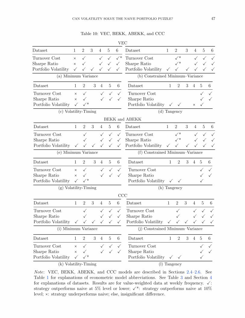
CAN VOLATILITY SOLVE THE NAIVE PORTFOLIO PUZZLE? 47
Table 10: VEC, BEKK, ABEKK, and CCC
VEC
Dataset 1 2 3 4 5 6
Turnover Cost × ✓ ✓ ✓ ✓*Sharpe Ratio × ✓ ✓ ✓ ✓Portfolio Volatility ✓ ✓ ✓ ✓ ✓ ✓
(a) Minimum Variance
Dataset 1 2 3 4 5 6
Turnover Cost ✓* ✓ ✓ ✓Sharpe Ratio ✓* ✓ ✓ ✓Portfolio Volatility ✓ ✓ ✓ ✓ ✓ ✓
(b) Constrained Minimum–Variance
Dataset 1 2 3 4 5 6
Turnover Cost × ✓ ✓ ✓ ✓Sharpe Ratio × ✓ ✓ ✓ ✓Portfolio Volatility ✓ ✓*
(c) Volatility-Timing
Dataset 1 2 3 4 5 6
Turnover Cost ✓ ✓Sharpe Ratio ✓ ✓Portfolio Volatility ✓ ✓ × ✓
(d) Tangency
BEKK and ABEKK
Dataset 1 2 3 4 5 6
Turnover Cost ✓ ✓ ✓ ✓Sharpe Ratio ✓ ✓ ✓ ✓Portfolio Volatility ✓ ✓ ✓ ✓ ✓ ✓
(e) Minimum Variance
Dataset 1 2 3 4 5 6
Turnover Cost ✓* ✓ ✓ ✓Sharpe Ratio ✓* ✓ ✓ ✓Portfolio Volatility ✓ ✓ ✓ ✓ ✓ ✓
(f) Constrained Minimum–Variance
Dataset 1 2 3 4 5 6
Turnover Cost × ✓ ✓ ✓ ✓Sharpe Ratio × ✓ ✓ ✓ ✓Portfolio Volatility ✓ ✓*
(g) Volatility-Timing
Dataset 1 2 3 4 5 6
Turnover Cost ✓ ✓Sharpe Ratio ✓ ✓Portfolio Volatility ✓ ✓ ✓
(h) Tangency
CCC
Dataset 1 2 3 4 5 6
Turnover Cost ✓ ✓ ✓ ✓Sharpe Ratio ✓ ✓ ✓ ✓Portfolio Volatility ✓ ✓ ✓ ✓ ✓ ✓
(i) Minimum Variance
Dataset 1 2 3 4 5 6
Turnover Cost ✓ ✓ ✓ ✓Sharpe Ratio ✓ ✓ ✓ ✓Portfolio Volatility ✓ ✓ ✓ ✓ ✓ ✓
(j) Constrained Minimum–Variance
Dataset 1 2 3 4 5 6
Turnover Cost × ✓ ✓ ✓ ✓Sharpe Ratio × ✓ ✓ ✓ ✓Portfolio Volatility ✓ ✓*
(k) Volatility-Timing
Dataset 1 2 3 4 5 6
Turnover Cost ✓ ✓Sharpe Ratio ✓ ✓Portfolio Volatility ✓ ✓ ✓
(l) Tangency
Note: VEC, BEKK, ABEKK, and CCC models are described in Sections 2.4–2.6. SeeTable 1 for explanations of econometric model abbreviations. See Table 3 and Section 4for explanations of datasets. Results are for value-weighted data at weekly frequency. ✓:strategy outperforms naive at 5% level or lower; ✓*: strategy outperforms naive at 10%level; ×: strategy underperforms naive; else, insignificant difference.
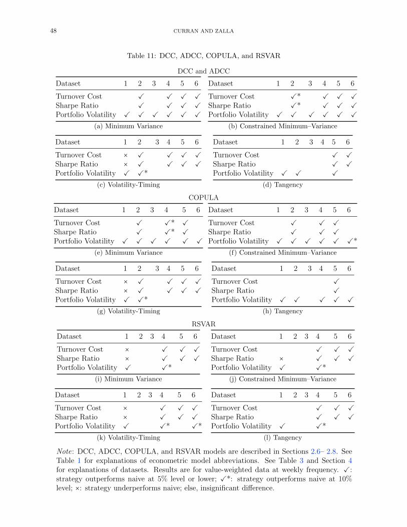
48 CURRAN AND ZALLA
Table 11: DCC, ADCC, COPULA, and RSVAR
DCC and ADCC
Dataset 1 2 3 4 5 6
Turnover Cost ✓ ✓ ✓ ✓Sharpe Ratio ✓ ✓ ✓ ✓Portfolio Volatility ✓ ✓ ✓ ✓ ✓ ✓
(a) Minimum Variance
Dataset 1 2 3 4 5 6
Turnover Cost ✓* ✓ ✓ ✓Sharpe Ratio ✓* ✓ ✓ ✓Portfolio Volatility ✓ ✓ ✓ ✓ ✓ ✓
(b) Constrained Minimum–Variance
Dataset 1 2 3 4 5 6
Turnover Cost × ✓ ✓ ✓ ✓Sharpe Ratio × ✓ ✓ ✓ ✓Portfolio Volatility ✓ ✓*
(c) Volatility-Timing
Dataset 1 2 3 4 5 6
Turnover Cost ✓ ✓Sharpe Ratio ✓ ✓Portfolio Volatility ✓ ✓ ✓
(d) Tangency
COPULA
Dataset 1 2 3 4 5 6
Turnover Cost ✓ ✓* ✓Sharpe Ratio ✓ ✓* ✓Portfolio Volatility ✓ ✓ ✓ ✓ ✓ ✓
(e) Minimum Variance
Dataset 1 2 3 4 5 6
Turnover Cost ✓ ✓ ✓Sharpe Ratio ✓ ✓ ✓Portfolio Volatility ✓ ✓ ✓ ✓ ✓ ✓*
(f) Constrained Minimum–Variance
Dataset 1 2 3 4 5 6
Turnover Cost × ✓ ✓ ✓ ✓Sharpe Ratio × ✓ ✓ ✓ ✓Portfolio Volatility ✓ ✓*
(g) Volatility-Timing
Dataset 1 2 3 4 5 6
Turnover Cost ✓Sharpe Ratio ✓Portfolio Volatility ✓ ✓ ✓ ✓ ✓
(h) Tangency
RSVAR
Dataset 1 2 3 4 5 6
Turnover Cost × ✓ ✓ ✓Sharpe Ratio × ✓ ✓ ✓Portfolio Volatility ✓ ✓*
(i) Minimum Variance
Dataset 1 2 3 4 5 6
Turnover Cost ✓ ✓ ✓Sharpe Ratio × ✓ ✓ ✓Portfolio Volatility ✓ ✓*
(j) Constrained Minimum–Variance
Dataset 1 2 3 4 5 6
Turnover Cost × ✓ ✓ ✓Sharpe Ratio × ✓ ✓ ✓Portfolio Volatility ✓ ✓* ✓*
(k) Volatility-Timing
Dataset 1 2 3 4 5 6
Turnover Cost ✓ ✓ ✓Sharpe Ratio ✓ ✓ ✓Portfolio Volatility ✓ ✓*
(l) Tangency
Note: DCC, ADCC, COPULA, and RSVAR models are described in Sections 2.6– 2.8. SeeTable 1 for explanations of econometric model abbreviations. See Table 3 and Section 4for explanations of datasets. Results are for value-weighted data at weekly frequency. ✓:strategy outperforms naive at 5% level or lower; ✓*: strategy outperforms naive at 10%level; ×: strategy underperforms naive; else, insignificant difference.
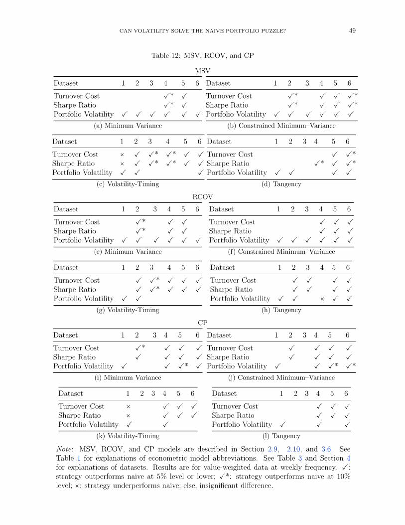
CAN VOLATILITY SOLVE THE NAIVE PORTFOLIO PUZZLE? 49
Table 12: MSV, RCOV, and CP
MSV
Dataset 1 2 3 4 5 6
Turnover Cost ✓* ✓Sharpe Ratio ✓* ✓Portfolio Volatility ✓ ✓ ✓ ✓ ✓ ✓
(a) Minimum Variance
Dataset 1 2 3 4 5 6
Turnover Cost ✓* ✓ ✓ ✓*Sharpe Ratio ✓* ✓ ✓ ✓*Portfolio Volatility ✓ ✓ ✓ ✓ ✓ ✓
(b) Constrained Minimum–Variance
Dataset 1 2 3 4 5 6
Turnover Cost × ✓ ✓* ✓* ✓ ✓Sharpe Ratio × ✓ ✓* ✓* ✓ ✓Portfolio Volatility ✓ ✓ ✓
(c) Volatility-Timing
Dataset 1 2 3 4 5 6
Turnover Cost ✓ ✓*Sharpe Ratio ✓* ✓ ✓*Portfolio Volatility ✓ ✓ ✓ ✓
(d) Tangency
RCOV
Dataset 1 2 3 4 5 6
Turnover Cost ✓* ✓ ✓Sharpe Ratio ✓* ✓ ✓Portfolio Volatility ✓ ✓ ✓ ✓ ✓ ✓
(e) Minimum Variance
Dataset 1 2 3 4 5 6
Turnover Cost ✓ ✓ ✓Sharpe Ratio ✓ ✓ ✓Portfolio Volatility ✓ ✓ ✓ ✓ ✓ ✓
(f) Constrained Minimum–Variance
Dataset 1 2 3 4 5 6
Turnover Cost ✓ ✓* ✓ ✓ ✓Sharpe Ratio ✓ ✓* ✓ ✓ ✓Portfolio Volatility ✓ ✓
(g) Volatility-Timing
Dataset 1 2 3 4 5 6
Turnover Cost ✓ ✓ ✓ ✓Sharpe Ratio ✓ ✓ ✓ ✓Portfolio Volatility ✓ ✓ × ✓ ✓
(h) Tangency
CP
Dataset 1 2 3 4 5 6
Turnover Cost ✓* ✓ ✓ ✓Sharpe Ratio ✓ ✓ ✓ ✓Portfolio Volatility ✓ ✓ ✓* ✓
(i) Minimum Variance
Dataset 1 2 3 4 5 6
Turnover Cost ✓ ✓ ✓ ✓Sharpe Ratio ✓ ✓ ✓ ✓Portfolio Volatility ✓ ✓ ✓* ✓*
(j) Constrained Minimum–Variance
Dataset 1 2 3 4 5 6
Turnover Cost × ✓ ✓ ✓Sharpe Ratio × ✓ ✓ ✓Portfolio Volatility ✓ ✓
(k) Volatility-Timing
Dataset 1 2 3 4 5 6
Turnover Cost ✓ ✓ ✓Sharpe Ratio ✓ ✓ ✓Portfolio Volatility ✓ ✓ ✓
(l) Tangency
Note: MSV, RCOV, and CP models are described in Section 2.9, 2.10, and 3.6. SeeTable 1 for explanations of econometric model abbreviations. See Table 3 and Section 4for explanations of datasets. Results are for value-weighted data at weekly frequency. ✓:strategy outperforms naive at 5% level or lower; ✓*: strategy outperforms naive at 10%level; ×: strategy underperforms naive; else, insignificant difference.