Can the Stolper-Samuelson Theorem explain relative wage movements?

Evidence from Mexico

Raymond Robertson

Department of EconomicsMacalester CollegeSt. Paul, MN 55105

robertson@macalester.edu

May 1999

Abstract: Rising wage inequality and increasing international trade have renewed interest in theempirical relevance of the Stolper-Samuelson theorem. Although a brilliant theoreticalaccomplishment, the Stolper-Samuelson theorem has received little empirical support. U.S. studieshave generated mixed results partially because prices are endogenous in a large country. This paperexamines the link between relative goods prices and relative wages in a small country: Mexico.This paper shows that on the eve of entering the GATT in 1986, Mexico protected less-skill-intensive industries. Trade liberalization caused dramatic movements in product prices. Startingfrom the initial pattern of protection, this paper then applies three approaches to comparing therelationship between product prices and relative wages against the predictions of the Stolper-Samuelson theorem. Following trade liberalization, the relative price of skill-intensive goods rose,raising the between-industry demand for skilled labor and the relative wages of skilled workers.All three approaches generate consistent empirical support for the Stolper-Samuelson theorem.The author thanks Antoni Estevadeordal, Gordon Hanson, Chihwa Kao, Mary Lovely, Dave Richardson, Matt Slaughter,M. Scott Taylor, Sarah West, and participants at the 1998 Empirical Investigations in International Trade conference forhelpful discussion and comments. All remaining errors are the sole responsibility of the author.

Can the Stolper-Samuelson Theorem explain relative wage movements?

Evidence from Mexico

Abstract: Rising wage inequality and increasing international trade have renewed interest in theempirical relevance of the Stolper-Samuelson theorem. Although a brilliant theoreticalaccomplishment, the Stolper-Samuelson theorem has received little empirical support. U.S.studies have generated mixed results partially because prices are endogenous in a large country.This paper examines the link between relative goods prices and relative wages in a small country:Mexico. This paper shows that on the eve of entering the GATT in 1986, Mexico protected less-skill-intensive industries. Trade liberalization caused dramatic movements in product prices.Starting from the initial pattern of protection, this paper then applies three approaches tocomparing the relationship between product prices and relative wages against the predictions ofthe Stolper-Samuelson theorem. Following trade liberalization, the relative price of skill-intensivegoods rose, raising the between-industry demand for skilled labor and the relative wages of skilledworkers. All three approaches generate consistent empirical support for the Stolper-Samuelsontheorem.

1

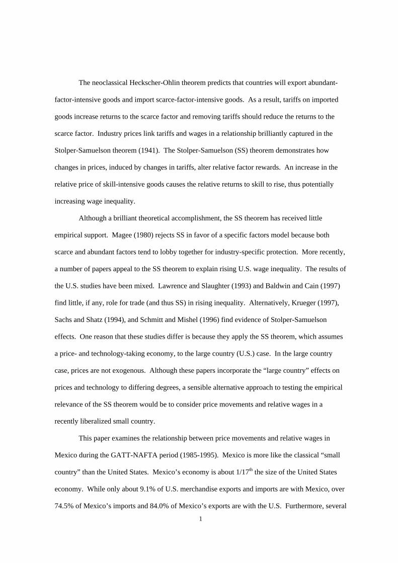
The neoclassical Heckscher-Ohlin theorem predicts that countries will export abundant-

factor-intensive goods and import scarce-factor-intensive goods. As a result, tariffs on imported

goods increase returns to the scarce factor and removing tariffs should reduce the returns to the

scarce factor. Industry prices link tariffs and wages in a relationship brilliantly captured in the

Stolper-Samuelson theorem (1941). The Stolper-Samuelson (SS) theorem demonstrates how

changes in prices, induced by changes in tariffs, alter relative factor rewards. An increase in the

relative price of skill-intensive goods causes the relative returns to skill to rise, thus potentially

increasing wage inequality.

Although a brilliant theoretical accomplishment, the SS theorem has received little

empirical support. Magee (1980) rejects SS in favor of a specific factors model because both

scarce and abundant factors tend to lobby together for industry-specific protection. More recently,

a number of papers appeal to the SS theorem to explain rising U.S. wage inequality. The results of

the U.S. studies have been mixed. Lawrence and Slaughter (1993) and Baldwin and Cain (1997)

find little, if any, role for trade (and thus SS) in rising inequality. Alternatively, Krueger (1997),

Sachs and Shatz (1994), and Schmitt and Mishel (1996) find evidence of Stolper-Samuelson

effects. One reason that these studies differ is because they apply the SS theorem, which assumes

a price- and technology-taking economy, to the large country (U.S.) case. In the large country

case, prices are not exogenous. Although these papers incorporate the “large country” effects on

prices and technology to differing degrees, a sensible alternative approach to testing the empirical

relevance of the SS theorem would be to consider price movements and relative wages in a

recently liberalized small country.

This paper examines the relationship between price movements and relative wages in

Mexico during the GATT-NAFTA period (1985-1995). Mexico is more like the classical “small

country” than the United States. Mexico’s economy is about 1/17th the size of the United States

economy. While only about 9.1% of U.S. merchandise exports and imports are with Mexico, over

74.5% of Mexico’s imports and 84.0% of Mexico’s exports are with the U.S. Furthermore, several

2

changes within Mexico created an excellent environment in which to study the SS theorem.

Mexico began to reduce trade barriers in 1986 when it rejected import substitution

industrialization and entered the General Agreement on Tariffs and Trade (GATT). Mexico

codified its commitment to trade liberalization by announcing intentions to enter into the North

American Free Trade Agreement (NAFTA) in 1990. NAFTA became effective January 1 1994.

Between 1985 and 1995, Mexico greatly reduced very high levels of trade protection.

As expected, trade liberalization had a dramatic and predictable effect on industry prices.

Mexico protected less-skill-intensive industries before entering the GATT and tariff reductions

were larger for less-skill-intensive industries. The impact on trade flows and relative wages was

also dramatic. Between 1987 and 1995, the annual sum of imports and exports divided by GDP

rose from 30% to 50%. Over the same period, wage inequality rose dramatically. The log-ratio of

non-production/production worker wages rose 55.9%. While the pattern of protection and changes

in relative wages have been shown by Revenga (1997) and Hanson and Harrison (1999), this paper

is the first to document a relationship between relative product prices and relative wages consistent

with the Stolper-Samuelson theorem.

To document the link between relative wages and relative prices, I rely on several sources

of data. First, I combine the Industrial Survey with detailed tariff data to document the pattern of

protection before liberalization according to factor intensity. To measure factor intensity, I

combine Mexico’s Monthly Industrial Survey with household-level survey data. This shows that

the skill breakdown in the Industrial Survey (production/non-production workers) is consistent

with other measures of skill (such as education). Next, I combine product-level price data with the

Industrial Survey to relate changes in relative prices with changes in relative wages.

To focus on the link between prices and wages, I follow the methods pioneered in what

Slaughter (1998) calls the "price studies". First, I follow Lawrence and Slaughter (1993), Krueger

(1997), and Sachs and Shatz (1994). If the SS theorem can explain rising relative wages of skilled

workers, then the relative price of skill-intensive goods must have risen. This "check" is a

necessary condition, and I find that it is satisfied in the Mexican case. Second, following

3

Francois, Navia, and Nelson (1998), I test for cointegration between relative wages and relative

prices. I only find weak evidence that month-to-month changes in relative wages are related to

changes in relative prices. This weak finding provides a response to Slaughter's (1998) question

"how fast does the SS clock tick" by suggesting slower-than-monthly adjustment. This result is

also consistent with Magee (1980) who finds that the SS theorem is more appropriate for long-run

adjustment. Third, I follow Baldwin and Cain (1997), Krueger (1997), Leamer (1998), Feenstra

and Hanson (1999), and Haskel and Slaughter (1999) and perform "mandated wage" regressions

that more closely relate to a formal derivation of the SS theorem. This approach uses factor

intensities and price changes to "predict" changes in wages that are consistent with SS. This

approach is problematic in U.S. studies because it assumes that prices and technology are

exogenous. These problems are at least partially obviated by examining the small country case. I

find that the predicted changes in wages are larger than actual changes, suggesting that SS forces

were more than sufficient to cause the observed change in wages.

Given the initial levels of protection and the pattern of liberalization, the results of all

three approaches provide consistent support for the SS theorem. Tariffs on less-skill-intensive

goods were higher and fell more. The relative price of these goods fell, causing a between-

industry shift towards skill-intensive industries. This increased the demand for skill and, in turn,

the relative wage of skilled workers.

The results of this paper further suggest that what matters for the relationship between

trade liberalization and wage inequality is the pattern of initial protection and not the perceived

relative factor endowments. Trade liberalization may induce rising inequality in developing

countries - even if they are less skill abundant - if the pattern of initial protection favored less-

skill-intensive industries. The resulting price changes, as demonstrated in this paper, affect

relative wages as the SS theorem predicts.

The paper unfolds in four sections. In Section I, I briefly review the formal derivation of

the SS theorem. The goal of the first section is to identify conditions that guide the rest of the

empirical analysis. In Section II, I describe the initial structure of protection and the pattern of

4

(4) ˆˆ Θwp =

liberalization, combining detailed tariff data with household and industrial surveys to classify

industries and protection according to factor intensity. In Section III, I evaluate the predictions of

the SS theorem described in the first section using the data described in the second section. I offer

conclusions in Section IV.

I. Predictions of the Stolper-Samuelson Theorem

The Stolper-Samuelson theorem is one of the most celebrated results in trade theory, and

the predictions are well known to trade theorists. Deardorff (1994) follows Jones (1964) by

demonstrating the SS theorem with the following simple general equilibrium model.

Consider an economy that produces n goods with m factors. Let w be an m-vector of

factor prices and let p be an n-vector of goods prices. If aij is the requirement of factor i to

produce one unit of good j, then let A(w) be the m by n matrix of these requirements chosen to

minimize unit production costs. It is also useful to define Θ as Deardorff does: the m by n

matrix of factor shares in which each element

θij = (wiaij)/pj. (1)

In practice, the unit labor requirement of labor of type i in good j will be calculated as

aij = Li/qj (2)

in which qj is the quantity of output in industry j. Thus, the elements of the factor share matrix are

calculated as the share of total revenues of good j that are paid to factor i.

Zero profits and perfect competition in equilibrium together imply

p = wA. (3)

The equation that provides the basis for empirical investigations of the SS theorem is derived by

totally differentiating (3) and making the necessary manipulations to generate

The “essential version” of the SS theorem is derived neatly when Θ is square and

invertable. The matrix Θ is inverted to yield a direct relationship between exogenous prices and

5

endogenous wages. However, most empirical studies use data from hundreds of industries while

considering at most four factors. Since the resulting Θ is not square and n > m > 2, the common

empirical response is an appeal to the Correlation Version of the Stolper-Samuelson Theorem

(Deardorff 1994). The Correlation Version acknowledges that, for a given change in the price

vector, it is impossible to say exactly which factor return will rise and which will fall. However,

there should be a correlation between the vectors of goods price changes and factor price changes.

Whether using the Correlation Version or a more strict interpretation, the literature has

identified four conditions that must hold to accredit SS forces with increasing wage inequality.

First, the prices of skill intensive goods must have risen relative to the prices of less-skill intensive

goods. This condition depends on the assumption of the small open economy because only in the

small open economy are prices considered exogenous. The second condition is that the output

shares of skill-intensive industries must have expanded. That is, in response to the change in

prices there was a between-industry shift in employment towards industries that use skilled labor

intensively.

The third is that the long-run relationship between relative prices and relative wages

should be positive. This condition lends itself to a time-series analysis. Slaughter (1998) asks

“how fast does the SS clock tick?” Applying various lag lengths to high-frequency data may

generate evidence that helps answer this question. The fourth and final condition is that, for a

given vector of factor shares, the wage changes predicted by the SS framework outlined above

should be equal to actual wage changes. If the predicted values fall short of the actual values, then

SS forces do not explain the changes in relative wages.

The papers that evaluate the price-wage relationship analyze these conditions. Early

papers in the debate focus on the first and second conditions. While Lawrence and Slaughter

(1993) find that relative prices of skill-intensive goods have fallen, Sachs and Shatz (1994) find

that relative prices have risen. Schmitt and Mishel (1996) and Krueger (1997) support the Sachs

and Shatz result. Francois, Navia, and Nelson (1998) evaluate the third condition. They argue that

(4) implies that prices and wages enjoy a long-run relationship. Thus, over time, prices and wages

6

should be cointegrated. They find evidence of a relationship between relative prices and relative

wages through time.

The fourth condition has also received recent attention. Cross-industry product-price

changes should be proportional to common-across-industries factor-price changes where the factor

of proportion is the industry’s factor shares. Leamer (1998) uses the term “mandated wage

equations” to describe the empirical forms estimated with this approach. The idea behind this

approach is that since the factor share matrix in (4) is not invertible, one can estimate (4) directly.

The wage vector is the set of parameters that are estimated when the vector of price changes across

time is regressed on the factor share matrix. The estimated vector is then compared to actual wage

changes. The next two sections analyze all four conditions in the Mexican case.

II. Tariffs, Relative Prices, and Relative Wages in Mexico, 1987-1995

In this section I describe the changes in Mexico’s trade policies and the changes in wage

inequality that followed. Next, I describe the data used for the empirical work, describe the

measures of skill, and conduct what Slaughter (1998) calls “consistency checks” for the relative

price movements. This section presents two key findings: Mexico protected less-skill-intensive

industries and, when protection was removed, the relative price of skill-intensive goods increased.

As a result, resources shifted between industries towards those that intensively employ skilled

labor.

A. The Structure of Protection in Mexico

Mexico turned from import substitution industrialization (ISI) in the early 1980s by

liberalizing foreign investment laws. The strongest sign of Mexico’s commitment to ending ISI

was its 1985 announcement to join the General Agreement on Tariffs and Trade (GATT). When

Mexico joined the GATT in 1986, it began to dramatically reduce trade barriers. Changes in

7

tariffs and quantity restrictions between 1985 and 1990 are reported in Table 1. Perhaps in

anticipation of the GATT, tariffs increased between 1984 and 1985. When Mexico joined the

GATT in 1986, tariffs dramatically fell until 1988, at which time they increased slightly and

stabilized.

Several authors have suggested that the structure of tariffs protected low-wage workers in

pre-reform Mexico (Revenga 1997, Hanson and Harrison 1999) and in other developing countries

(Currie and Harrison 1997). To examine this hypothesis, I first calculate one common measure of

factor intensity, the non-production/production worker ratio, for each industry (in subsequent

sections, I add and compare other measures of skill intensity, but these are not available for 1985).

The relative employment data come from the 1985 Mexican Industrial Census, the closest census

to the 1986 reforms. The census employment data are matched to the average most-favored-nation

(MFN) tariff rates for Mexico in 1985.1 As noted earlier, tariffs increased between 1984 and 1985

and then fell until 1988.

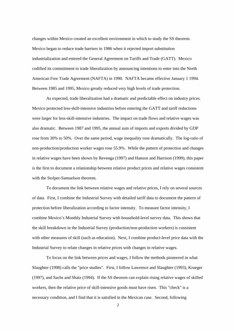
Figure 1 graphs the 1985 MFN tariff rates as a function of the relative employment of non-

production to production workers. The fitted lines are estimated with and without weights (using

total industry employment as weights). The estimated slope (standard error) is -17.388 (8.311)

without weights and -25.795 (7.862) with weights. There is a clear negative relationship between

1985 tariff levels and the share of non-production workers. This affirms Hanson and Harrison

(1999) and others who find that the pre-reform structure of tariffs protected less-skilled workers.

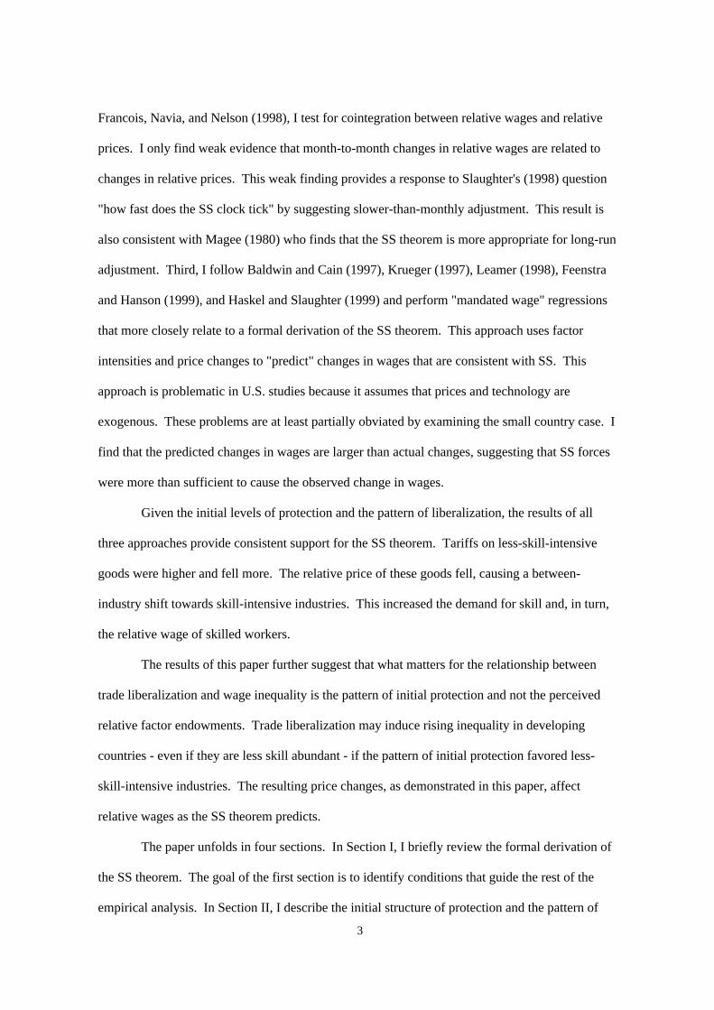
Figure 2 shows the change in tariffs as a function of relative employment. The unweighted slope

(standard error) is 13.329 (7.050) and the weighted slope (standard error) is 18.428 (6.787). These

results also are consistent with Hanson and Harrison: industries that intensively use production

workers experienced larger tariff declines.

1 I thank Antoni Estevadeordal of the IADB for the tariff data. The tariff data are the unweighted averagemost favored nation (mfn) applied tariff rates. The census employment data were aggregated to the 4-digitISIC Rev. 2 level to match the tariff data.

8

B. The Rise in Wage Inequality

As in other developing countries (Robbins 1995), trade liberalization in Mexico was

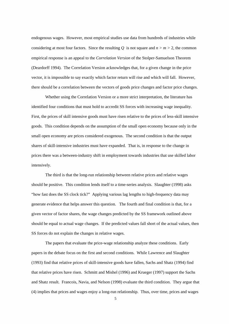
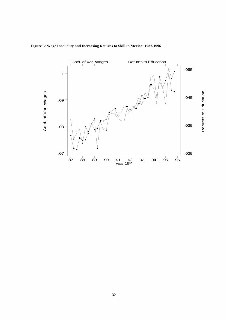
accompanied by an increase in wage inequality. Figure 3 presents data from the Mexican

National Urban Employment Survey (or ENEU, from its Spanish acronym) from eight Mexican

metropolitan areas2 and shows both the coefficient of variation of log wages and the return to

education for each quarter between 1987 and 1995.3 The rise in the return to education follows the

coefficient of variation of log wages rather closely.4 These findings are consistent with those of

Cragg and Epelbaum (1996), Revenga (1997), and Hanson and Harrison (1999).5 These papers

attribute the rise in wage inequality to a rising demand for skill.

The Stolper-Samuelson theorem attributes a rise in wage inequality to an increase in the

demand for skill between industries. To calculate the relative importance of between and within

industry changes in demand for skill, I turn to the Mexican Monthly Industrial Survey (Encuesta

Industrial Mensual, or EIM). The survey covers 3,172 manufacturing firms in 129 4-digit classes

of industrial activity. The National Institute of Geography, Information, and Statistics (INEGI)

conducts the survey. The survey is used to construct indicators of industrial activity. The data

exclude firms in the maquiladora industry6 and firms with less than 6 employees. The data do

not include information on temporary or unpaid workers (in 1988, unpaid workers made up only

about 10% of manufacturing employment).7

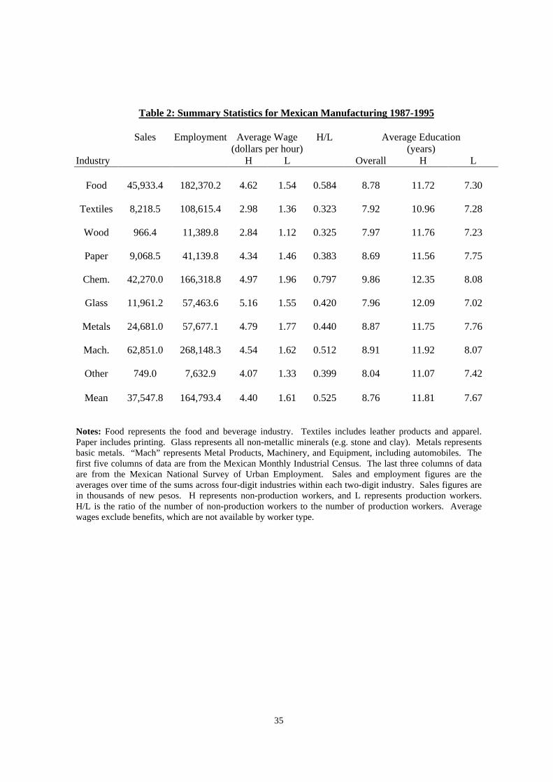
Table 2 contains the summary statistics from the EIM by two-digit industry. There are

significant differences in average hourly wages across industries that are not generally stable

2 Mexico City, Mexico State, Monterrey, Guadalajara, Tijuana, Ciudad Juarez, Nuevo Laredo, andMatamoros.3 Data for earlier years are not available.4 The return to education was estimated as the coefficient on a continuous years-of-education variable from alog-wage equation using the pooled ENEU data. Separate equations were estimated for each quarter.5 Currency movements also influenced relative prices, confounding the effects of tariff changes. Mexico'speso was devalued in 1987, making imports more expensive and afforded import-competing industries somerelief from the reduction in trade barriers. The peso's ill-fated overvaluation began to accelerate after 1990,and the trade balance took a sharp negative turn. The tariff reductions would have been "felt" more stronglyafter 1990.

9

through time (Cragg and Epelbaum 1996, Robertson 1999a). These differentials are incorporated

explicitly in subsequent sections. The largest industries, both in terms of employment and sales,

are Machinery, Food Products, and Chemicals. Chemicals, Food Products, and Metal Products

have the highest non-production/production employment ratios.8,9 I follow Lawrence and

Slaughter (1993) and divide the 127 industries into those that intensively use production workers

and those that intensively use non-production workers. As mentioned earlier, use of the

production/non-production distinction as a proxy for skill intensity has been criticized in U.S.

studies. However, in Mexico this distinction seems to capture much of the skill segregation within

industries. The last three columns in Table 2 use ENEU data to show that production workers

have less education in every industry than non-production workers. Industries with higher relative

employment ratios also have higher average education levels. Both Kendall and Pearson rank-

correlation tests reject the hypothesis that the two measures (education and the non-

production/production ratio) are independent at the 0.0001 level. Using the production/non-

production distinction to (imperfectly) classify skill intensity seems valid in the Mexican case.

I classify those with non-production/production employment ratios above the median in

each period as non-production-worker intensive. The change in the ratio of non-production

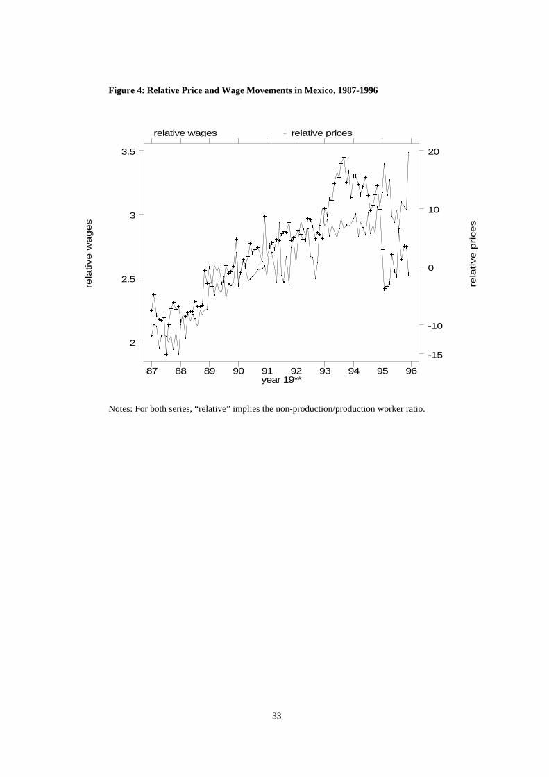
(higher skilled) to production worker (less skilled) wages is shown in Figure 4. The change in

relative wages mimics those found in Figure 3. The ratio increases from about 2.5 to over 3 during

the 1987-1995 period.10

6 The maquiladora industry, or in-bond industry, is composed of the group of plants allowed to import partsfor assembly duty-free and then export the finished product. Tariffs are only paid on value added in Mexico.These firms are included in the firm-level surveys used later in this paper.7 Unpaid workers include apprentices and family members.8 Mexico also has a higher share of total employment in these industries than the U.S. (see Robertson1999a).9 While the computer industry remains problematic in U.S. price studies of the early 1980s, it is not anoutlier in the Mexican data. Therefore, I do not control separately for the computer industry in the analysisthat follows. Slaughter (1998) argues that the computer industry should not be excluded even if it is an“outlier” because, as such, it may contain important information.10 Blonigen and Slaughter (1999) find that in the U.S. over the 1979-1994 period, the non-production/production worker wage ratio rose from 1.52 to 1.67.

10

∑+∑=j

jjj

jj seesE ∆∆∆

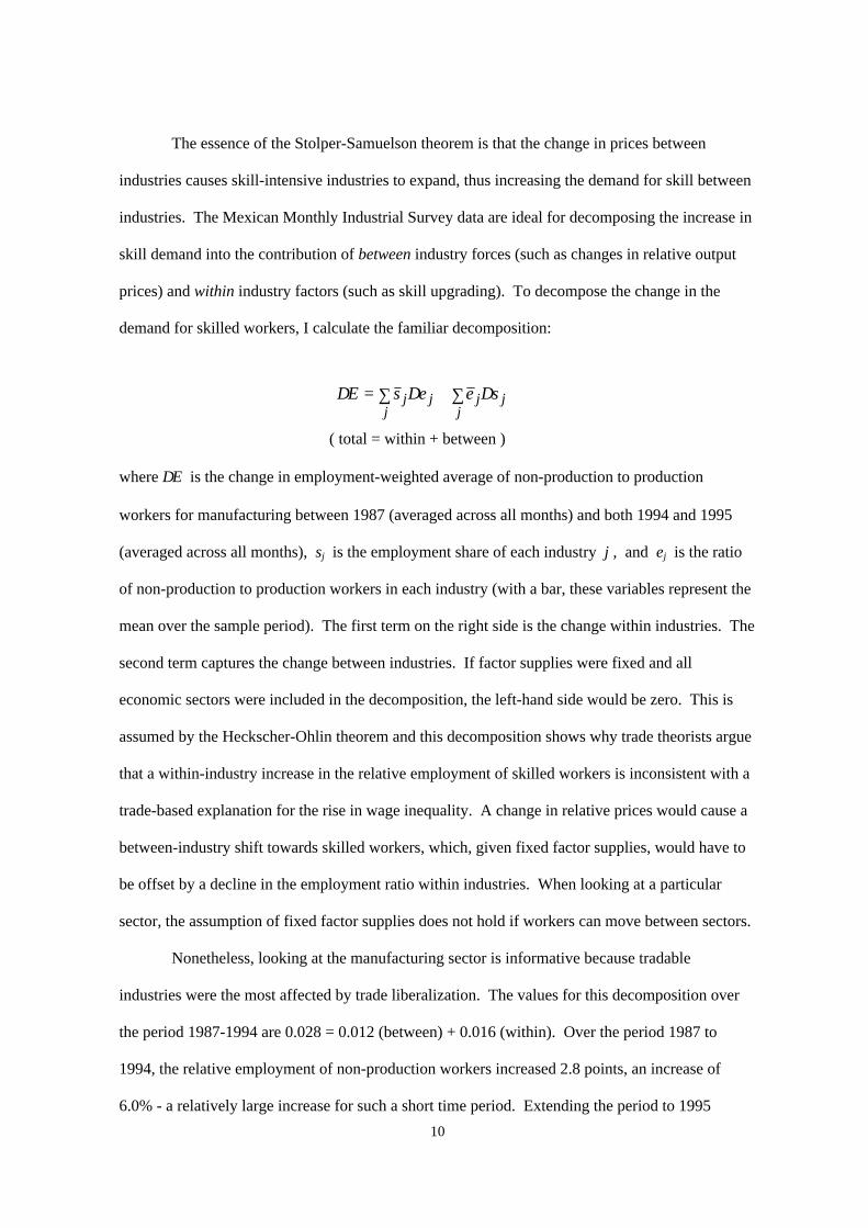
The essence of the Stolper-Samuelson theorem is that the change in prices between

industries causes skill-intensive industries to expand, thus increasing the demand for skill between

industries. The Mexican Monthly Industrial Survey data are ideal for decomposing the increase in

skill demand into the contribution of between industry forces (such as changes in relative output

prices) and within industry factors (such as skill upgrading). To decompose the change in the

demand for skilled workers, I calculate the familiar decomposition:

( total = within + between )

where ∆E is the change in employment-weighted average of non-production to production

workers for manufacturing between 1987 (averaged across all months) and both 1994 and 1995

(averaged across all months), sj is the employment share of each industry j , and ej is the ratio

of non-production to production workers in each industry (with a bar, these variables represent the

mean over the sample period). The first term on the right side is the change within industries. The

second term captures the change between industries. If factor supplies were fixed and all

economic sectors were included in the decomposition, the left-hand side would be zero. This is

assumed by the Heckscher-Ohlin theorem and this decomposition shows why trade theorists argue

that a within-industry increase in the relative employment of skilled workers is inconsistent with a

trade-based explanation for the rise in wage inequality. A change in relative prices would cause a

between-industry shift towards skilled workers, which, given fixed factor supplies, would have to

be offset by a decline in the employment ratio within industries. When looking at a particular

sector, the assumption of fixed factor supplies does not hold if workers can move between sectors.

Nonetheless, looking at the manufacturing sector is informative because tradable

industries were the most affected by trade liberalization. The values for this decomposition over

the period 1987-1994 are 0.028 = 0.012 (between) + 0.016 (within). Over the period 1987 to

1994, the relative employment of non-production workers increased 2.8 points, an increase of

6.0% - a relatively large increase for such a short time period. Extending the period to 1995

11

produces 0.041 = 0.021 (between) + 0.019 (within). Over the 1987-1995 period the relative

employment of skilled workers in manufacturing increased over 8%. The decomposition reveals

that the change in skill demand over the 1987-1994 period was about equally divided between

between and within effects.11

III. The Role of Stolper-Samuelson Effects

This section employs three approaches to evaluate the hypothesis that Stolper-Samuelson

forces can explain relative price movements in Mexico. In part A, I perform simple “consistency

checks” for conditions that must hold if SS forces are at work. In part B, I employ time-series

techniques to test whether relative wages and relative prices are cointegrated. In part C, I apply

the mandated wage approach first proposed by Baldwin and Hilton (1984) and recently applied by

Baldwin and Cain (1997), Leamer (1998), Feenstra and Hanson (1999) and Haskel and Slaughter

(1999). All three approaches provide evidence supporting the Stolper-Samuelson theorem in the

Mexican case.

A. Necessary and Sufficient Conditions for Stolper-Samuelson Effects

The first condition of the Stolper-Samuelson theorem involves relative price movements.

Did the relative price of production- or non-production-worker-intensive goods increase? There

are two approaches to this question. As in Lawrence and Slaughter (1993), I regress the change in

prices (dPj) over the sample period on the ratio of non-production to production workers (H/L) at

the beginning of the sample period:

dPj = α+ β(H/L)j + ej . (5)

11 Robertson (1999b) evaluates the hypothesis that the within industry component of skill upgrading was a

12

To estimate (5) I use survey output data and product-price data. The price data are

collected in the industrial survey but are collected at the product level. I aggregate product level

prices to the four-digit industry level. Following Hanson and Harrison (1999), I deflate the price

data with the Mexican CPI. Details of the construction of the price data are found in the

Appendix.

Table (3) presents the regression results for the Mexican data for the period following

trade liberalization.12 The effect of price changes may be sensitive to endpoints because Mexico

experienced currency devaluations in 1987 and 1995. The North American Free Trade Agreement

between Canada, the United States, and Mexico went into effect in January 1994. I present four

regressions for each of three measures of skill intensity. Each column in Table 3 contains the

results from a separate regression using different endpoints (1987-1995, 1988-1995, 1987-1994,

and 1988-1994). Each regression is estimated using weighted least squares using the mean value

of output over 1987-1995 as weights.13 The first four rows contain the results from regressions of

the change in relative price on the 1987 mean ratio of non-production to production workers. All

of point estimates are positive and two are significant. These results suggest that the output price

of skill-intensive industries increased relative to less-skill-intensive industries following trade

liberalization.

In the second panel of rows in Table 3, I apply Krueger's (1997) measure of skill intensity:

the employment share of production workers. The results are consistent with those in the first

panel of Table 3. Industries with higher shares of production workers had smaller price changes.

The last panel further corroborates this finding (though more weakly) using average education

levels of the workers within each industry, calculated using household-level data. All of the

result of the effects of international factors on the firm’s technology choice.12 Using U.S. data and without controlling for the computer industry, Lawrence and Slaughter (1993) findeither a negative or zero estimate for β and conclude that the relative price of non-production workerintensive goods did not increase over the sample period. Using a similar approach, Sachs and Shatz (1994)control for the computer industry and find a positive correlation. Krueger (1997) uses U.S. data from 1989-1995 and finds a positive correlation with and without controlling for the computer industry. Slaughter(1998) discusses the robustness of results found with and without computer-industry controls.13 Krueger (1997) uses weights and Slaughter (1998) discusses the robustness of using weights. They areappropriate for the Mexican case because of the large variance in industry employment.

13

coefficients are positive and one is statistically significant. Industries with higher average levels

of education had greater price changes over the sample period.

Another way to examine the changes in prices and factor intensities is to take advantage of

the panel aspect of the data. Analyzing the between-industry price movements and relative

employment over time also reveals whether changes in relative prices were higher for more non-

production-worker-intensive industries. Table 4 shows the (weighted) between industry

regressions of

lnPij = α+ β ln(H/L)ij + eij (6)

lnPij = α+ β ln(L/(H+L))ij + eij (7)

lnPij = α+ β ln(education)ij + eij (8)

The between-industry regressions in equations (6) - (8) is equivalent to a regression on the

means within industries (over time). A positive coefficient in (6), for example, suggests that, on

average, industries with higher non-production/production worker ratios experienced larger

increases in prices. The results in Table 4 suggest that there is a significant and positive

relationship between skill intensity and the change in the output price. This evidence indicates that

the relative price of non-production-worker-intensive goods rose relative to the price of

production-worker-intensive goods. The results are robust to using different measures of skill

intensity; the results from equation (8) are very similar to the results from equations (6) and (7).

The next condition is not strictly necessary for the presence of Stolper-Samuelson effects

but, if present, plays a very important role. As an industry’s relative output price increases, that

industry’s output share should also increase (thus increasing the demand for factors employed in

that industry). As a first step to testing this prediction, I perform a fixed-effects panel regression

of both the output share and employment share on industry output price with and without a time

trend. The effects of prices on output and employment share are found in Table 5. Industries 3512

(agricultural and hand tools) and 3820 (construction and repair of rail equipment) lack price data

14

it1iti0it py εβαα +++= −

and are dropped. The regressions include a fixed effect for 126 of 127 four-digit industries. That

is, I perform the regression:

(9)

in which yit is either the output share (the value of output in industry i in period t divided by the

sum of the value of output across all 4-digit industries within period t ) or the employment share

(constructed in the same way as the output share).

Table 5 shows that, as expected, both output and employment shares positively respond to

price increases. The coefficient on log industry price is positive and significant, suggesting that,

on average, a 10% increase in the price index (relative to the CPI) increases the industry output

share by 4.1% the industry employment share by 1.6%. This result should not be surprising since

it is consistent with the simplest model of competitive, price-taking firms with rising marginal

costs.

Results in Tables 3-5 demonstrate a between-industry shift in employment towards non-

production-worker-intensive industries.14 Price changes favored non-production-worker intensive

industries and these industries expanded as a result. This between-industry shift raised the demand

for non-production workers. If the labor supply curve is not horizontal, this increase in demand

would raise the relative wages of non-production workers.

These results suggest that Mexican tariffs protected less-skill-intensive industries, that the

relative price of skill-intensive goods increased when those tariffs were reduced, and, as a response

to the change in relative prices, the skill-intensive industries expanded. Together, the findings

from the previous section are consistent with the SS theorem, but do not directly support the

relationship represented in (4). Ideally, solving equation (4) for wages as functions of prices and

estimating these functions would determine the effect of changes in prices on wages, but

14 Regressing the change in the employment share on a dummy variable that is equal to 1 if the industry isproduction worker intensive also generates a negative and significant coefficient (results available from theauthor upon request).

15

1ˆˆ −= Θpw

dimensionality makes solving (4) difficult. Specifically, (4) can only be solved when there are an

equal number of goods and factors and even then it does not give clear results when the number of

goods and factors exceeds two. One solution to this problem is addressed with the time-series

approach discussed in the next section.

B. A Time Series Approach

Using two classifications of workers (skilled and unskilled), Francois, Navia, and Nelson

(1998) circumvent the dimensionality problem by dividing industries into two groups based on

factor intensity. Since there are only two factors (skilled and unskilled workers) and only two

goods (based on factor intensity), the factor share matrix in (4) can be inverted to yield

(10)

which Francois, Navia, and Nelson interpret as representing the relationship between relative

prices and relative wages over time.

Francois, Navia, and Nelson follow Borjas and Ramey (1994) and Baldwin and Cain

(1997) when constructing their relative wage series, and when computing relative prices. They

then test the hypothesis that relative wages and relative prices are cointegrated. There are two

necessary conditions for cointegration. The first is that both series must exhibit a unit root. The

second is that the difference between the two series be stationary. Only if the first condition is

satisfied is the second condition considered. Francois, Navia, and Nelson find weak evidence that

the two series exhibit a unit root and then weak evidence that the relative wages and relative prices

are cointegrated. However, they admit that their results are not very robust across various lag

structures.

To perform a similar analysis with the Mexican data, I classify the Mexican manufacturing

industries into two groups based on the median ratio of production to non-production workers.

16

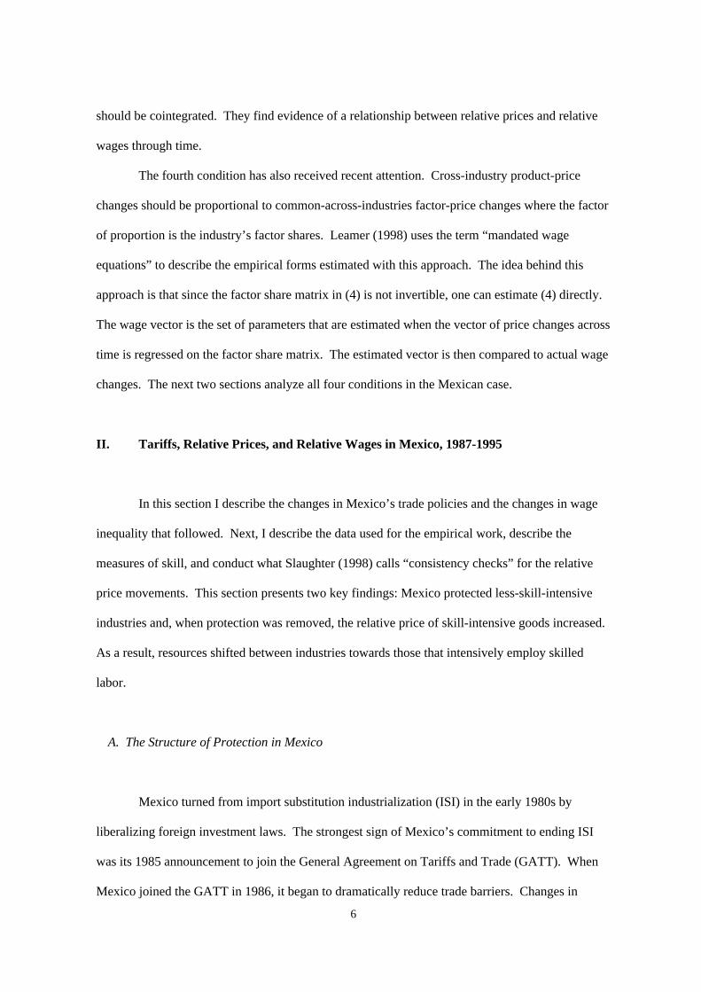
Using this classification, I then calculate the production-weighted ratio of the output price indices

of the two groups. Since the data already include wages for production and non-production

workers, I calculate the employment-weighted relative wage. Figure (4) graphs the movements of

relative prices and relative wages. The two series follow closely together throughout the sample

period until NAFTA went into effect in 1994.15

While Figure (4) seems to suggest that the two variables are closely related over time,

each condition for cointegration must be considered. I first use the root mean squared error of the

regression (RMSE), Akaike's Information Criterion (AIC), Amemiya's Prediction Criterion (PC),

and Schwarz's Information Criterion (SC) to determine each variable’s optimal lag length. Given

these lag lengths, I then apply the augmented Dickey-Fuller unit root test for each variable. Since

the test statistics (p-values) are -2.11 (0.242) and -2.39 (0.145), I fail to reject the hypothesis that

each series exhibits a unit root.16

The next step is to test for cointegration. I follow the Engle-Granger approach as

described in Engle and Yoo (1987). The Engle-Granger approach tests the stationarity of the

residuals of

lnwt = α + β ln pt + zt (11)

in which wt represents the ratio of non-production worker wages to production worker wages and

pt represents the ratio of the price of non-production-worker intensive goods to production-

worker-intensive goods. Again using the augmented Dickey-Fuller test for stationarity, the test

statistic (p-value) is -1.15 (0.870) which indicates a failure to reject the null of no cointegration.

15 The apparent structural change that takes place when NAFTA went into effect may not be surprising.When Mexico joined the GATT in 1986, it significantly lowered trade barriers to the rest of the world. Interms of factor endowments, Mexico may look very different to the United States and Canada than it does tothe rest of the world. Furthermore, by joining NAFTA, Mexico may have reduced protection for a differentset of industries than it reduced for the GATT. While further exploration of the effects of NAFTA vs.GATT is interesting, it is beyond the scope of the present paper.16 Including a trend did not affect the qualitative results.

17

Even though the two series are not cointegrated, it is still interesting to extend the

Francois, Navia, and Nelson analysis and perform (4) with monthly data because the Stolper-

Samuelson theorem (and the trade theorists single-cone response to factor-content studies)

suggests that relative prices drive relative wages. Time series techniques can be used to test this

facet of the trade/wages relationship.

OLS estimation results of (10) generate a coefficient (standard error) of relative prices of

1.418 (0.262). While this would seem to be consistent with the Stolper-Samuelson theorem, the

resulting Durbin-Watson statistic (0.344) suggests that the error terms are serially correlated. In

the presence of adjustment costs for employment and wages, the error terms would be serially

correlated if lagged dependent variables, which capture the persistence of changes, were omitted

from the regression. Table 6 contains the results of estimating (4) with a more complex lag

structure. Three lags of wages are sufficient to eliminate the serial correlation as shown by

Dubin’s h statistic in Table 6. To examine the effects of prices, I also include 6 and 12 lags of the

relative prices (with and without a time trend). The results in Table 6 show that when serial

correlation is corrected, the first lagged price coefficient is negative. Up until the last lags (6 or

12), the pattern is oscillating. The test for Granger causality, which is a test that the price

coefficients are jointly zero, also fails to reject the hypothesis that short-run price changes drive

wages.

The long run-effects, while measured imprecisely, are positive in every case in Table 6.17

The net effect of prices on wages is greater than one. This result is consistent with the Jones

(1965) magnification effect that suggests that the change in wages following a price change will be

larger than the change in prices. Of course, the earlier finding of a unit root in both series casts

doubt on these results.

17 Including a time trend significantly dampens the long-run effect of prices. Including the time trend doesnot follow from the Stolper-Samuelson theorem and thus the results with the time trend should be takenlightly.

18

Given the fact that the data were found to have a unit root, I next take the first difference

of both series to make them stationary. The regression results for the differenced series are found

in Table 7. The results are qualitatively similar to those in Table 6. The first lagged difference of

prices has a negative effect on the change in relative wages, but the second lag has a stronger,

positive effect. In all cases, the long-run effects of changes in prices (the sum of the coefficients)

are positive although less than one and statistically insignificant. The trend term is not statistically

significant in the differenced-data regressions and does not affect the results.

Overall, the time series results provide weak evidence that monthly price variation drives

changes in relative wages. The imprecision of the estimates may not be surprising given several

strict assumptions necessary to perform this approach. For example, the approach assumes

minimal adjustment costs. In the presence of adjustment costs, factors may not respond rapidly

enough for SS forces to be detected in the high-frequency data. That is, the Stolper-Samuelson

“clock” may tick less than once a month. Furthermore, the results in Tables 6 and 7 provide the

effects of a single shock to prices on wages. That result, while positive, is very noisy. However,

Mexico did not experience just one price shock. Tariffs and import controls were relaxed over a

period of several years. Figure (3) suggests that relative prices followed a long upward trend.

Taken together, the sum of the individual changes in relative wages may have had significant

effects.

C. The Mandated Wage Approach

The time series results are consistent with the hypothesis that price shocks drive relative

wages, but factors need time to adjust. Given the sustained rise in relative prices that occurred in

Mexico, the mandated wage approach may capture the cumulative effect of the changes in relative

prices that took place over the 10-year period. Mandated wage equations test the relationship

between the change in prices and the change in wages over long time periods (generally nine or ten

years).

19

To test the long-run relationship between wages and prices, the mandated wage approach

compares predicted changes in wages with actual changes. The accuracy of the predictions

provides information about the determinants of wage movements. If the predicted changes match

the actual changes, then Stolper-Samuelson effects are said to have a large contributing role in

determining wages. If the match is poor, then the direction of the difference suggests other factors,

such as changes in technology. Consistent with previous sections, I find that the mandated wage

approach predicts increasing wage inequality in Mexico.

This approach has been contentious in the U.S. and the literature has identified four key

estimation issues. The first concerns the exogeneity of price changes. The SS theorem assumes

that prices are exogenous. The application of this approach to the U.S. has generated conflicting

results for the United States. This should not be surprising if the world market does not determine

U.S. prices, as the SS theorem assumes. The advantage of studying the small country is that prices

and technology are assumed to be exogenous. The price changes that followed the tariff changes

seem to strongly support the exogeneity of price changes in Mexico during this time period

because relatively larger tariff reductions on less-skill-intensive goods were followed by relatively

larger price reductions on less-skill-intensive goods. Nonetheless, I test the robustness of the

results to controls for endogeneity found in U.S. studies.

The second issue has not been addressed in most wage studies. As Lawrence (1999) and

Haskel and Slaughter (1999) point out, trade may cause technical improvements that affect the

relative demand for skill. Thus, trade may contribute to within-industry skill upgrading. This

issue is addressed directly by Robertson (1999b) and thus is not fully addressed here. What must

be addressed for the purposes of this paper is the assumption that technology is exogenous. There

is considerable evidence that Mexican firms do take technology as given. In 1992, INEGI

conducted a firm-level survey of 5071 manufacturing firms.18

18 The National Survey of Employment, Salaries, Technology, and Training in the Manufacturing Sector(Encuesta Nacional de Empleo, Salarios, Tecnologia, Capacitacion en el Sector Manufactuero, 1992) was ajoint project between INEGI, Mexico’s Labor Secretariat, and the OIT.

20

The survey includes questions about technology investment and acquisition. According to

the survey, the average share of revenues allocated for research and development was 0.6% in

1992 while the average share of revenues allocated for technology purchases was 3.1% in 1992

(up from 2.5% in 1989).19 64% of firms with more than 100 workers purchased their technology

from abroad and over 37% purchased their technology directly from the United States.

Furthermore, only 2.6% of all firms in the survey reported using a “cutting-edge” productive

process, with the rest having either a “mature” or “older” process. Given that Mexico is a

developing country that tends to import technology, it seems reasonable to assume that

technological improvements are first realized by the developed countries, affect prices in the

developed countries, and then get passed to the developing countries both directly and through

product prices. I make that assumption in the empirical work that follows.

The third estimation issue involves value-added prices. Slaughter (1998) shows that

intermediate inputs make up large and growing shares of production in the U.S. Accounting for

the prices of intermediate inputs is especially important when intermediate inputs are imported

because changes in the prices of intermediate inputs are passed through to product prices and can

thus affect factor prices (Woodland 1982). Unfortunately, the industrial survey data do not include

information on intermediate inputs. Thus, when using the industrial survey data, I am forced to

use “gross” output prices rather than “net” output prices. To check the robustness of these results,

I introduce information on intermediate inputs from the Mexican Industrial Census. The

correlation between the value-added prices changes and the gross-output price changes in 0.9033.

The findings are qualitatively robust to using value-added prices and accounting for intermediate

inputs.

Feenstra and Hanson (1999) introduced the fourth estimation issue. They argue that when

total factor productivity and changes in inter-industry wage differentials (iiwds) are introduced

into the mandated wage equations, the equations become an identity. In Haskel and Slaughter’s

19 For comparison, on average, U.S. industry spent 3.1% of net sales on R&D in 1989 (National ScienceFoundation, 1992).

21

jiji ij ewp ++= ∑ θα

(1999) study of U.K. wage inequality, they argue that iiwds are stable in Great Britian and so do

not affect the analysis. Neither Feenstra and Hanson nor Haskel and Slaughter control for

differences in demographic characteristics when examining iiwds. Controlling for demographic

characterisics with household-level survey data, Robertson (1999a) finds that iiwds are not stable

in Mexico over the 1987-1995 period. However, when changes in iiwds are incorporated into the

Mexican mandated wage regressions, the equation does not behave in the same way as Feenstra

and Hanson find (i.e. the equation does not behave as an identity). Nonetheless, the findings are

qualitatively similar when iiwds are included, as discussed in detail in the following paragraphs.

Baldwin and Cain (1997) interpret (4) with the following regression equation:

(12)

in which i is the factor index and θ is the share of factor i employed in industry j . The variables

pj and wi represent the output price in industry j and the economy-wide return to factor i

respectively. The circumflexes (^) indicate percentage changes. In this approach, the factor shares

are the independent variables and the prices are the endogenous variables. In this sense, the

estimation deviates from a strict interpretation of the theory. The parameters to be estimated are

the changes in the wages (over the sample period) that are assumed to be equal across all industries

because factors are assumed to be perfectly mobile across industries.

I estimate equation (12) using the average factor shares in 1987 and the change in the

output price index for each industry using the same four endpoints and samples as in the earlier

analysis. The regression includes 127 manufacturing industries. As in Baldwin and Cain, I use

the value of industry output as regression weights.

The actual changes in average hourly wages and the results from (12) are found in Table 8.

There is a clear difference between the mandated change in wages for production and non-

production workers in all regressions. The predicted change in wages for production workers is

large and negative while the predicted change in non-production wages is large and positive. In all

22

cases, the predicted changes in wages are larger than the actual changes. In only one case are the

predicted changes statistically different from the actual changes (production workers over the

1988-1995 period). In this case, the predicted change in wages is large and negative, while the

actual change is close to zero. While the large standard errors may suggest that the null hypothesis

(that predicted changes and actual changes are similar) is difficult to reject, the actual wage change

for non-production workers is outside the 95% confidence interval for the predicted wage of

production workers in all four cases. Although somewhat imprecise at times, all of the point

estimates are consistent with the Stolper-Samuelson theorem and the predicted changes are similar

to the actual changes.

Although the results in Table 8 support the Stolper-Samuelson theorem, there are several

reasons to be concerned about the results. First, as noted earlier, the survey data used for these

results do not include intermediate inputs, such as capital and materials. The Mexican Industrial

Census contains these data for 54 four-digit industries for 1985, 1988, and 1993. Price data from

the Survey concord with 45 of the Census industries for 1988 and 1993. The Census data allow

me to construct value-added price measures by multiplying the price index by (1 - share of

materials). Results from estimating (12) with the Census data and value-added prices are found in

Table 9. The first two columns use the actual cost shares of the factors and the second two

columns constrain the cost shares to sum to one. In columns (1) and (3) the dependent variable is

the change in value-added prices over the 1988-1993 period. In columns (2) and (4) the dependent

variable is the change in value-added prices over the 1987-1994 period (using the 1988 and 1993

data to construct value-added prices for 1987 and 1994).

When unconstrained, the mandated wage changes suggest that wage inequality should

have decreased with very large drops in non-production worker wages. When constrained, the

estimated coefficients suggest that the wage inequality should have increased. Constrained factor

shares seem to provide a more intuitive representation of factor intensity, but these contrasting

results suggest that the mandated wage approach is sensitive to specification. One possible reason

for this sensitivity is omitted variable bias. One key candidate for such a variable is technology.

23

In Table 10, I include two measures of technology. The first two columns show results when the

difference between the change in output and the change in factor inputs (the common measure of

total factor productivity) is included in the mandated wage equation. Feenstra and Hanson (1999)

argue that the specification of the mandated wage equation is made complete (and thus the

mandated wage equation becomes and identity) when technology is adjusted for changes in inter-

industry wage differentials.

Including technology improves the fit of all equations, but the adjusted R2 never

approaches the 0.999 the Feenstra and Hanson (1999) find with U.S. data, although the

methodology used here is the same. Changes in technology enter significantly in all equations

suggesting that prices rose in industries that had larger gains in technology.20 When technology is

included, the predicted change in wages is much closer to those actually observed in Mexico. This

is especially true in column (1). Point estimates in all four columns in Table (4) are consistent

with the Stolper-Samuelson theorem in that they all “mandate” larger changes in non-production

wages and smaller (indeed in two cases negative) changes in production-worker wages. The

coefficients are not measured very precisely, and the necessary aggregation to the census data may

contribute to the imprecision. Nonetheless, the point estimates are consistent with the results

generated with the Survey data (once technology changes are accounted for).

The Stolper-Sameulson forces suggested by the mandated wage equations suggest that the

change in relative prices would have caused an even larger increase in wage dispersion had other

factors not been at work. Measures designed to protect low-wage workers, not uncommon in

Mexico, may have been in effect and deserve further exploration.21

20 There are many reasons to question causality running from technology to prices. For example, severalpapers have found that positive demand shocks (rising output prices) are correlated with large productivitygains and they attribute this to labor hoarding. See, for example, Anton and Evans (1998).21 Bell finds (1997) minimum wages may not contribute to the explanation. Other possibilities include wageagreements between business, labor, and the government that established an effective floor above the legalminimum.

24

IV. Conclusions

Using data from a small, recently liberalized economy, this paper compares movements in

prices and wages against the predictions of the Stolper-Samuelson theorem. The current literature

suggests that four conditions must hold to accredit SS forces with changes in relative wages. First,

the prices of skill intensive goods must have risen relative to the prices of less-skill intensive

goods. Second, the output shares of skill-intensive industries must have expanded. Third, the

long-run relationship between relative prices and relative wages should be positive. Fourth, for a

given vector of factor shares, the wage changes predicted by the SS framework outlined above

should be equal to actual wage changes. If the predicted values fall short of the actual values, then

SS forces do not explain the changes in relative wages.

This paper finds evidence supporting all four conditions in the Mexican case. The rising

relative prices of skill-intensive goods led to the expansion of skill-intensive industries, thus

increasing the demand for skilled labor. Using both a time-series analysis and the “mandated

wage” approach, this paper also finds that rising wage inequality could be explained by rising

relative prices. Since all four conditions are satisfied, this paper provides strong and consistent

support for the Stolper-Samuelson explanation for wage movements in Mexico.

Why did Mexico initially protect less-skill-intensive industries? This pattern of protection

seems to pose a challenge to the Heckscher-Ohlin theorem. Wood (1997) suggests that relative to

the Asian countries, Mexico may not be relatively abundant in less-skilled workers. In any case,

this paper suggests that, given the pattern of initial protection and reduction in trade barriers, price

changes seem to have driven the wage changes in this small country case, as the Stolper-

Samuelson theorem predicts.

These findings also support those who argue that trade could have affected U.S. wages to

the extent that this paper supports the Stolper-Samuelson theorem. Attempts to control for the

endogeneity of technology and prices seem to be an appropriate way to adapt the Stolper-

Samuelson theorem to the large country case.

25

Appendix A: Construction of the Price Data

The product-level price data used in this study are from the Mexican Instituto Nacional deEstadistica, Geographia, e Informatica (INEGI). There are, on average, 25 products per 4-digitindustry for a total of 947 products. The price data are computed as unit values from value andvolume data and then aggregated into averages across 4-digit industries. For each industry Iconstructed both the Laspeyeres (base-year quantities) and Paasche (current quantities) priceindices. There are relatively few differences between the two measures. For the empirical work inthis paper I used the arithmetic average of the two indices.

One issue that arose with the construction of the price indices is that quantities for someproducts were not available. As a result, unit values and price indices could not be computed overall available products in the industry. In most cases the share of the excluded products in the totalindustry value is relatively small. For industries missing quantities for certain goods, I constructedthe price indices from available unit prices. As noted in the text, I dropped industries with no priceinformation.

INEGI constructs and publishes price indices for the two-digit industry level. To test forrobustness, I also used these measures in place of the 4-digit constructed price indices. The resultsare qualitatively similar but, as expected, the two-digit price indices exhibit much smallervariance.

26

Appendix B: ISIC Rev. 2 Codes

ISICRev2 Description3111 Slaughtering, preparing and preserving meat3112 Manufacture of dairy products3113 Canning and preserving of fruits and vegetables3114 Canning, preserving and processing of fish, crustacea and similar foods3115 Manufacture of vegetable and animal oils and fats3116 Grain mill products3117 Manufacture of bakery products3118 Sugar factories and refineries3119 Manufacture of cocoa, chocolate and sugar confectionery3121 Manufacture of food products not elsewhere classified3122 Manufacture of prepared animal feeds3131 Distilling, rectifying and blending spirits3132 Wine industries3133 Malt liquors and malt3134 Soft drinks and carbonated waters industries3140 Tobacco manufactures3211 Spinning, weaving and finishing textiles3212 Manufacture of made-up textile goods except wearing apparel3213 Knitting mills3214 Manufacture of carpets and rugs3215 Cordage, rope and twine industries3219 Manufacture of textiles not elsewhere classified3220 Manufacture of wearing apparel, except footwear3231 Tanneries and leather finishing3232 Fur dressing and dyeing industries3233 Manufacture of products of leather and leather substitutes, except footwear and wearing apparel3240 Manufacture of footwear, except vulcanized or moulded rubber or plastic footwear3311 Sawmills, planing and other wood mills3312 Manufacture of wooden and cane containers and small cane ware3319 Manufacture of wood and cork products not elsewhere classified3320 Manufacture of furniture and fixtures, except primarily of metal3411 Manufacture of pulp, paper and paperboard3412 Manufacture of containers and boxes of paper and paperboard3419 Manufacture of pulp, paper and paperboard articles not elsewhere classified3420 Printing, publishing and allied industries3511 Manufacture of basic industrial chemicals except fertilizers3512 Manufacture of fertilizers and pesticides3513 Manufacture of synthetic resins, plastic materials and man-made fibres except glass3521 Manufacture of paints, varnishes and lacquers3522 Manufacture of drugs and medicines3523 Manufacture of soap and cleaning preparations, perfumes, cosmetics and other toilet preparations3529 Manufacture of chemical products not elsewhere classified3530 Petroleum refineries3540 Manufacture of miscellaneous products of petroleum and coal3551 Tyre and tube industries3559 Manufacture of rubber products not elsewhere classified3560 Manufacture of plastic products not elsewhere classified3610 Manufacture of pottery, china and earthenware3620 Manufacture of glass and glass products3691 Manufacture of structural clay products3692 Manufacture of cement, lime and plaster3699 Manufacture of non-metallic mineral products not elsewhere classified3710 Iron and steel basic industries3720 Non-ferrous metal basic industries3811 Manufacture of cutlery, hand tools and general hardware

27

Appendix B: ISIC Rev. 2 Codes (continued)

ISICRev2 Description3812 Manufacture of furniture and fixtures primarily of metal3813 Manufacture of structural metal products3819 Manufacture of fabricated metal products except machinery and equipment n.e.c.3820 Manufacture of engines and turbines3822 Manufacture of agricultural machinery and equipment3823 Manufacture of metal and woodworking machinery3824 Manufacture of special industrial mach. and equip. except metal and - woodworking mach.3825 Manufacture of office, computing and accounting machinery3829 Machinery and equipment except electrical not elsewhere classified3831 Manufacture of electrical industrial machinery and apparatus3832 Manufacture of radio, television and communication equipment and apparatus3833 Manufacture of electrical appliances and housewares3839 Manufacture of electrical apparatus and supplies not elsewhere classified3841 Shipbuilding and repairing3842 Manufacture of railroad equipment3843 Manufacture of motor vehicles3844 Manufacture of motorcycles and bicycles3845 Manufacture of aircraft3849 Manufacture of transport equipment not elsewhere classified3851 Manufacture of professional and scientific, and measuring and controlling equipment, n.e.c.3852 Manufacture of photographic and optical goods3853 Manufacture of watches and clocks3901 Manufacture of jewellery and related articles3902 Manufacture of musical instruments3903 Manufacture of sporting and athletic goods3909 Manufacturing industries not elsewhere classified

28

References

Anton, B. and Evans, C. (1998) “Seasonal Solow Residuals and Christmas: A Case for Labor Hoarding andIncreasing Returns” Journal of Money, Credit, and Banking 30(3, Pt. 1) August, pp. 306-30.

Baldwin, R. and Cain, G. (1997) "Shifts in U.S. Relative Wages: The Role of Trade, Technology, and FactorEndowments" NBER Working Paper No. 5934.

Baldwin, R. and Hilton, R. (1984) “A Technique for Indicating Comparative Costs and Predicting Changesin Trade Ratios” Review of Economics and Statistics 66(1) February, pp. 105-10.

Bell, L. (1997) “The Impact of Minimum Wages in Mexico and Colombia” Journal of Labor Economics;15(3, Pt. 2), pp. S102-35.

Blonigen, B. and Slaughter, M. (1999) “Foreign-Affiliate Activity and U.S. Skill Upgrading” NBERWorking Paper No. W7040.

Borjas, G. and Ramey, V. (1994) "Time-Series Evidence on the Sources of Trends in Wage Inequality"American Economic Review; 84(2) May, pp. 10-16.

Cragg, M. and Epelbaum, M. (1996) “Why Has Wage Dispersion Grown in Mexico? Is it the Incidence ofReforms or the Growing Demand for Skills?” Journal of Development Economics 51, pp. 99-116.

Currie, J. and Harrison, A. (1997) “Sharing the Costs: The Impact of Trade Reform on Capital and Labor inMorocco” Journal of Labor Economics 15(3 Pt. 2) July, pp. S44-71.

Deardorff, A. (1994) “Overview of the Stolper-Samuelson Theorem” in Deardorff, A. and Stern, R. (eds.)The Stolper-Samuelson Theorem: A Golden Jubilee University of Michigan Press, Ann Arbor, pp. 7-34.

Engle, R. and Yoo, B. (1987) “Forecasting and Testing in Co-integrated Systems” Journal of Econometrics35(1), May, pp. 143-59.

Feenstra, R. and Hanson, G. (1999) “The Impact of Outsourcing and High-technology Capital on Wages:Estimates for the United States: 1979-1990” forthcoming, Quarterly Journal of Economics.

Findlay, R. (1995) Factor Proportions, Trade, and Growth The MIT Press, Cambridge, MA.

Francois, J. Navia, R. and Nelson, D. (1998) "Treating the SS theorem Seriously: The Long-RunRelationship between Relative Commodity Prices and Relative Factor Prices" mimeo, ErasmusUniversity.

Hanson, G. and Harrison, A. (1999) "Trade, Technology, and Wage Inequality" forthcoming, Industrial andLabor Relations Review 52(2) January, pp. 271-88.

Haskel, J. and Slaughter, M. (1999) “Trade, Technology, and U.K. Wage Inequality” NBER working paperNo. 6978.

Jones, R. (1965) “The Structure of Simple General Equilibrium Models” Journal of Political Economy 73,pp. 557-72.

Krueger, A. (1997) "Labor Market Shifts and the Price Puzzle Revisited" NBER Working Paper No. 5924.

29

Lawrence, R. (1999) “Does a Kick in the Pants Get You Going, or Does it Just Hurt You? The Impact ofInternational Competition on Technical Change in U.S. Manufacturing”, forthcoming in R.C. Feenstra(ed.) International Trade and Wages Cambridge: NBER.

Lawrence, R. and Slaughter, M. (1993) "International Trade and American Wages in the 1980s: GiantSucking Sound or Small Hiccup?" Brookings Papers: Microeconomics 2, pp. 161-226.

Leamer, E. (1998) “In Search of Stolper-Samuelson Linkages between Trade and Lower Wages” in Collins,S. (ed.) Imports, Exports, and the American Worker Brookings Institute Press, pp. 141-202.

Magee, S. (1980) "Three Simple Tests of the Stolper-Samuelson Theorem" as found in Deardorff, A. andStern, R. (eds.) The Stolper-Samuelson theorem: A golden jubilee. Studies in International TradePolicy. Ann Arbor: University of Michigan Press, 1994, pp. 185-200.

National Science Foundation (1992) “Research and Development in Industry, 1989” NSF 92-307,Washington, D.C. Government Printing Office.

Revenga, A. (1997) "Employment and Wage Effects of Trade Liberalization: The Case of MexicanManufacturing" Journal of Labor Economics, 15(3, pt. 2), pp. S20-S43.

Robbins, D. (1995) “Trade, Trade Liberalisation, and Inequality in Latin America and East Asia: Synthesisof Seven Country Studies,” Harvard Institute for International Development, Cambridge, Mass.Processed.

Robertson, R. (1999a) “Inter-industry Wage Differentials Across Time, Borders and Trade Regimes:Evidence from the US and Mexico” mimeo, Syracuse University.

Robertson, R. (1999b) “Trade or Technology? Why Not Both? Evidence on Technology Choice, WageInequality, and International Trade” mimeo, Syracuse University.

Sachs, J. and Shatz, H. (1994) "Trade and Jobs in U.S. Manufacturing" Brookings Papers on EconomicActivity I, pp. 1-84.

Schmitt, J. and Mishel, L. (1996) "Did International Trade Lower Less-Skilled Wages During the 1980s?Standard Trade Theory and Evidence" Economic Policy Institute Technical Paper No. 213.

Slaughter, M. (1998) "What Are the Results of Product-Price Studies and What Can We Learn From theDifferences?" NBER working paper No. 6591.

Stolper, W. and Samuelson, P. (1941) “Protection and Real Wages” Review of Economic Studies 9November, pp. 58-73.

Wood, A. (1997) “Openness and Wage Inequality in Developing Countries: The Latin American Challengeto East Asian Conventional Wisdom” World Bank Economic Review 11(1) January, pp. 33-57.

Woodland, A.D. (1982) International Trade and Resource Allocation North-Holland, Amsterdam.

30

Figure 1: AverageTariff Levels and Relative Employment: 1985

Notes: The graph plot points are the ISIC Rev. 2 Industry Codes. Relative size reflects totalindustry employment. Employment data are from the 1985 Mexican Industrial Census.

Non-prod./Prod. Employment.2 .4 .6 .8 1

0

20

40

60

80

31113112

31133114

3115

3116

3117

3118

3119

3121

31223131

3132

3133

3134

3140

3211

3212 3213

3215

3220

3231

32333240

3311

3320

3411

3412

3420

35113512

3513

3521

3522

3523

3529

3540

3551

3560

3610

3620

3691 3692

3699

37103720

38113812

3813

3819

3822

3823 3824

3825

3829

38313832

3833

3841

3842

3843

3844

3851

3852

3901

3909

MFN

Tar

iff

Rat

es

Unweighted

Weighted

31

Figure 2: Tariff Changes and Relative Employment: 1985-1988

Notes: The graph plot points are the ISIC Rev. 2 Industry Codes. Relative size reflects totalindustry employment. Employment data are from the 1985 Mexican Industrial Census.

Non-prod./Prod. Employment.2 .4 .6 .8 1

-60

-40

-20

0

3111

3112

31133114

3115

3116

3117

3118

31193121

3122

3131

3132

3133

3134

3140

3211

3212

3213

3215

3220

3231

3233

3240

3311

33203411

3412

3420

35113512

3513

3521

3522

3523

35293540

3551

3560

3610

3620

3691

3692

3699

37103720

3811

3812

3813

3819

38223823

3824

3825

3829

38313832

3833

3841

3842

3843

3844

3851

3852

3901

3909

Cha

nge

in T

arif

fs, 1

985-

1988

weighted

unweighted

32

Figure 3: Wage Inequality and Increasing Returns to Skill in Mexico: 1987-1996C

oe

f. o

f V

ar.

Wa

ge

s

year 19**

Re

turn

s t

o E

du

ca

tio

n

Coef. of Var. Wages Returns to Education

87 88 89 90 91 92 93 94 95 96

.07

.08

.09

.1

.025

.035

.045

.055

33

Figure 4: Relative Price and Wage Movements in Mexico, 1987-1996

Notes: For both series, “relative” implies the non-production/production worker ratio.

rela

tive

wa

ge

s

year 19**

rela

tive

price

s

relative wages relative prices

87 88 89 90 91 92 93 94 95 96

2

2.5

3

3.5

-15

-10

0

10

20

34

Table 1: Average Tariffs and Import-License Requirements by Two-Digit Industry, 1984-1990 (%)

Industry H/L 1984 1985 1986 1987 1988 1989 1990

Food 0.584 42.9 45.4 32.1 22.9 14.8 15.8 16.2

Textiles 0.323 38.6 43.2 40.4 26.6 16.8 16.6 16.7

Wood 0.325 47.3 48.5 44.9 29.9 17.7 17.6 17.8

Paper 0.383 33.7 36.5 34.8 23.7 7.7 10.1 9.9

Chem. 0.797 29.1 29.9 27.0 20.5 13.4 14.3 14.4

Glass 0.420 37.1 38.5 33.8 22.4 13.8 14.3 14.3

Metals 0.440 13.6 16.7 18.4 13.8 7.9 11.0 11.0

Mach. 0.512 43.1 46.3 30.0 20.8 14.1 15.9 16.1

Other 0.399 40.9 42.9 40.5 27.5 17.1 18.1 18.4

Notes: Source: Hanson and Harrison, 1999, except for the second column. In the second column, H/L is theratio of the number of non-production workers to the number of production workers and is identical tocolumn (H/L) in Table 3. Food represents the food and beverage industry. Textiles includes leatherproducts and apparel. Paper includes printing. Glass represents all non-metallic minerals (e.g. stone andclay). Metals represents basic metals. “Mach” represents Metal Products, Machinery, and Equipment,including automobiles.

35

Table 2: Summary Statistics for Mexican Manufacturing 1987-1995

Sales Employment Average Wage(dollars per hour)

H/L Average Education(years)

Industry H L Overall H L

Food 45,933.4 182,370.2 4.62 1.54 0.584 8.78 11.72 7.30

Textiles 8,218.5 108,615.4 2.98 1.36 0.323 7.92 10.96 7.28

Wood 966.4 11,389.8 2.84 1.12 0.325 7.97 11.76 7.23

Paper 9,068.5 41,139.8 4.34 1.46 0.383 8.69 11.56 7.75

Chem. 42,270.0 166,318.8 4.97 1.96 0.797 9.86 12.35 8.08

Glass 11,961.2 57,463.6 5.16 1.55 0.420 7.96 12.09 7.02

Metals 24,681.0 57,677.1 4.79 1.77 0.440 8.87 11.75 7.76

Mach. 62,851.0 268,148.3 4.54 1.62 0.512 8.91 11.92 8.07

Other 749.0 7,632.9 4.07 1.33 0.399 8.04 11.07 7.42

Mean 37,547.8 164,793.4 4.40 1.61 0.525 8.76 11.81 7.67

Notes: Food represents the food and beverage industry. Textiles includes leather products and apparel.Paper includes printing. Glass represents all non-metallic minerals (e.g. stone and clay). Metals representsbasic metals. “Mach” represents Metal Products, Machinery, and Equipment, including automobiles. Thefirst five columns of data are from the Mexican Monthly Industrial Census. The last three columns of dataare from the Mexican National Survey of Urban Employment. Sales and employment figures are theaverages over time of the sums across four-digit industries within each two-digit industry. Sales figures arein thousands of new pesos. H represents non-production workers, and L represents production workers.H/L is the ratio of the number of non-production workers to the number of production workers. Averagewages exclude benefits, which are not available by worker type.

36

Table 3: Price Changes and Initial Skill Intensities

87-95 88-95 87-94 88-94

H/L 0.091 0.080 0.194 0.199(0.057) (0.061) (0.052) (0.057)

intercept -0.239 -0.178 -0.404 -0.362(0.037) (0.040) (0.034) (0.037)

adj. R-sq. 0.013 0.006 0.098 0.087N 117 117 117 117

L/(H+L) -0.312 -0.267 -0.634 -0.652(0.186) (0.201) (0.171) (0.187)

intercept 0.021 0.046 0.131 0.188(0.128) (0.139) (0.118) (0.129)

adj. R-sq. 0.015 0.007 0.098 0.088N 117 117 117 117

Education 0.042 0.061 0.008 0.023(0.022) (0.024) (0.022) (0.024)

intercept -0.579 -0.706 -0.371 -0.464(0.208) (0.222) (0.204) (0.220)

adj. R-sq. 0.021 0.047 -0.008 -0.001N 117 117 117 117

Notes: H represents non-production workers. L represents productionworkers. Education is measured in years. The 129 industries in theIndustrial Survey were aggregated into the 117 identifiable industries in thehousehold level data. Standard errors are in parentheses.

37

Table 4:Between-Industry Regressions of Prices on Skill Measures

ln(H/L) ln(L/(H+L)) ln(av. educ)

skill 0.072 -0.232 0.109(0.010) (0.026) (0.011)

cons 4.656 4.506 4.367(0.023) (0.019) (0.032)

chi-sq 10656.72 10661.12 9821.23p-value 0.000 0.000 0.000

N 13715 13715 12791

Notes: H represents non-production workers. L represents productionworkers. Education is measured in years. Results are generated withStata®’s xtgee command (generalized estimation equation) with 107time effects (all months in the 1987 to 1995 period, less one) andweighted by the average output value. The dependent variable is theoutput price index. Standard errors are in parentheses.

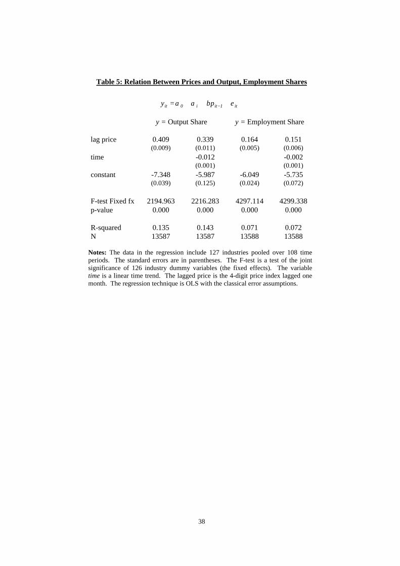
38

it1iti0it py εβαα +++= −

Table 5: Relation Between Prices and Output, Employment Shares

y = Output Share y = Employment Share

lag price 0.409 0.339 0.164 0.151(0.009) (0.011) (0.005) (0.006)

time -0.012 -0.002(0.001) (0.001)

constant -7.348 -5.987 -6.049 -5.735(0.039) (0.125) (0.024) (0.072)

F-test Fixed fx 2194.963 2216.283 4297.114 4299.338p-value 0.000 0.000 0.000 0.000

R-squared 0.135 0.143 0.071 0.072N 13587 13587 13588 13588

Notes: The data in the regression include 127 industries pooled over 108 timeperiods. The standard errors are in parentheses. The F-test is a test of the jointsignificance of 126 industry dummy variables (the fixed effects). The variabletime is a linear time trend. The lagged price is the 4-digit price index lagged onemonth. The regression technique is OLS with the classical error assumptions.

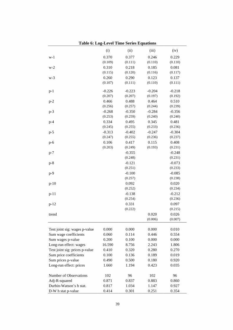
39

Table 6: Log-Level Time Series Equations

(i) (ii) (iii) (iv)

w-1 0.370 0.377 0.246 0.229(0.109) (0.111) (0.110) (0.110)

w-2 0.310 0.218 0.185 0.081(0.115) (0.120) (0.116) (0.117)

w-3 0.260 0.290 0.123 0.137(0.107) (0.111) (0.110) (0.111)

p-1 -0.226 -0.223 -0.204 -0.218(0.207) (0.207) (0.197) (0.192)

p-2 0.466 0.488 0.464 0.510(0.256) (0.257) (0.244) (0.239)

p-3 -0.268 -0.350 -0.284 -0.356(0.253) (0.259) (0.240) (0.240)

p-4 0.334 0.495 0.345 0.481(0.245) (0.255) (0.233) (0.236)

p-5 -0.313 -0.402 -0.247 -0.304(0.247) (0.255) (0.236) (0.237)

p-6 0.106 0.417 0.115 0.408(0.203) (0.249) (0.193) (0.231)

p-7 -0.355 -0.248(0.248) (0.231)

p-8 -0.121 -0.073(0.251) (0.233)

p-9 -0.100 -0.085(0.257) (0.238)

p-10 0.092 0.020(0.252) (0.234)

p-11 -0.138 -0.212(0.254) (0.236)

p-12 0.331 0.097(0.222) (0.215)

trend 0.020 0.026(0.006) (0.007)

Test joint sig: wages p-value 0.000 0.000 0.000 0.010Sum wage coefficients 0.060 0.114 0.446 0.554Sum wages p-value 0.200 0.100 0.000 0.000Long-run effect: wages 16.590 8.756 2.243 1.806Test joint sig: prices p-value 0.410 0.320 0.280 0.270Sum price coefficients 0.100 0.136 0.189 0.019Sum prices p-value 0.490 0.500 0.180 0.920Long-run effect: prices 1.660 1.194 0.423 0.035

Number of Observations 102 96 102 96Adj-R-squared 0.871 0.837 0.883 0.860Durbin-Watson’s h stat. 0.817 1.034 1.147 0.927D-W h stat p-value 0.414 0.301 0.251 0.354

40

Table 7: Log-Differenced Time Series Equations

(i) (ii) (iii) (iv)

w-1 -0.565 -0.487 -0.563 -0.487(0.110) (0.117) (0.111) (0.119)

w-2 -0.245 -0.257 -0.243 -0.257(0.122) (0.125) (0.123) (0.127)

w-3 0.095 0.130 0.098 0.130(0.113) (0.119) (0.115) (0.121)

p-1 -0.180 -0.127 -0.174 -0.127(0.207) (0.215) (0.210) (0.220)

p-2 0.255 0.326 0.261 0.326(0.206) (0.212) (0.210) (0.217)

p-3 0.053 -0.017 0.061 -0.017(0.215) (0.221) (0.220) (0.227)

p-4 0.405 0.465 0.410 0.465(0.204) (0.215) (0.207) (0.222)

p-5 0.035 -0.060 0.038 -0.060(0.200) (0.220) (0.202) (0.225)

p-6 0.463 0.487 0.468 0.487(0.193) (0.213) (0.195) (0.223)

p-7 0.046 0.046(0.217) (0.226)

p-8 0.004 0.004(0.217) (0.232)

p-9 -0.119 -0.119(0.218) (0.231)

p-10 -0.012 -0.012(0.215) (0.227)

p-11 -0.238 -0.238(0.208) (0.216)

p-12 0.048 0.048(0.219) (0.224)

trend 0.000 0.000(0.002) (0.002)

Test joint sig: wages p-value 0.000 0.000 0.000 0.000Sum wage coefficients 1.715 1.613 1.707 1.614Sum wages p-value 0.000 0.000 0.000 0.000Long-run effect: wages 0.583 0.620 0.586 0.620Test joint sig: prices p-value 0.100 0.290 0.100 0.300Sum price coefficients 1.030 0.804 1.064 0.803Sum prices p-value 0.130 0.500 0.130 0.550Long-run effect: prices 0.601 0.498 0.623 0.498

Number of Observations 101 95 101 95Adj-R-squared 0.304 0.275 0.297 0.266Durbin-Watson’s h stat. 0.209 1.721 0.076 2.055D-W h stat p-value 0.835 0.085 0.939 0.04

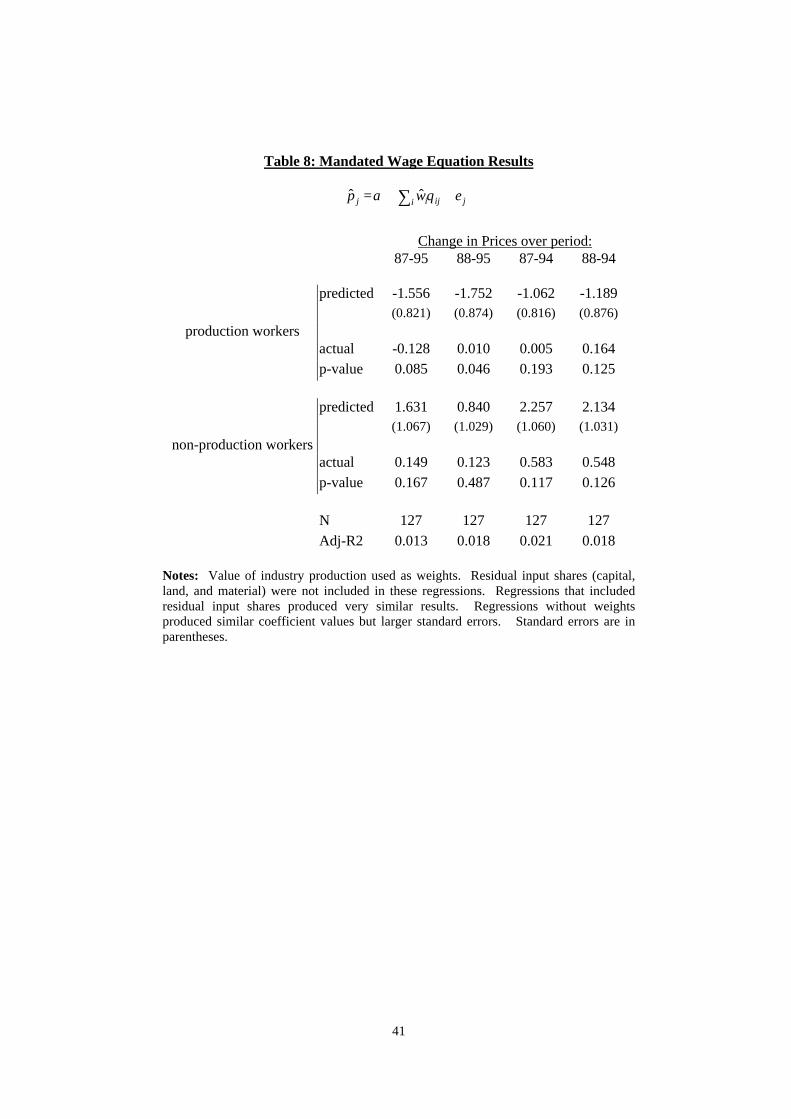
41

jiji ij ewp ++= ∑ θα ˆ ˆ

Table 8: Mandated Wage Equation Results

Change in Prices over period:87-95 88-95 87-94 88-94

predicted -1.556 -1.752 -1.062 -1.189(0.821) (0.874) (0.816) (0.876)

production workersactual -0.128 0.010 0.005 0.164p-value 0.085 0.046 0.193 0.125

predicted 1.631 0.840 2.257 2.134(1.067) (1.029) (1.060) (1.031)

non-production workersactual 0.149 0.123 0.583 0.548p-value 0.167 0.487 0.117 0.126

N 127 127 127 127Adj-R2 0.013 0.018 0.021 0.018

Notes: Value of industry production used as weights. Residual input shares (capital,land, and material) were not included in these regressions. Regressions that includedresidual input shares produced very similar results. Regressions without weightsproduced similar coefficient values but larger standard errors. Standard errors are inparentheses.

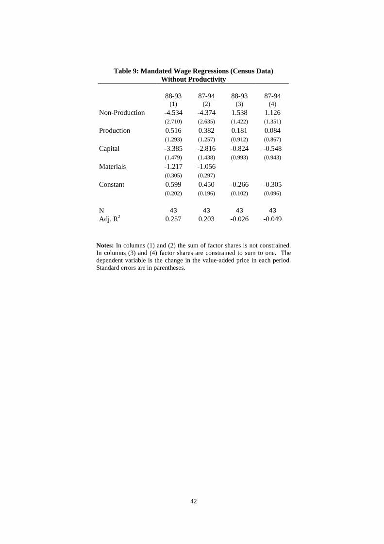
42

Table 9: Mandated Wage Regressions (Census Data)Without Productivity

88-93 87-94 88-93 87-94(1) (2) (3) (4)

Non-Production -4.534 -4.374 1.538 1.126(2.710) (2.635) (1.422) (1.351)

Production 0.516 0.382 0.181 0.084(1.293) (1.257) (0.912) (0.867)

Capital -3.385 -2.816 -0.824 -0.548(1.479) (1.438) (0.993) (0.943)

Materials -1.217 -1.056(0.305) (0.297)

Constant 0.599 0.450 -0.266 -0.305(0.202) (0.196) (0.102) (0.096)

N 43 43 43 43Adj. R2 0.257 0.203 -0.026 -0.049

Notes: In columns (1) and (2) the sum of factor shares is not constrained.In columns (3) and (4) factor shares are constrained to sum to one. Thedependent variable is the change in the value-added price in each period.Standard errors are in parentheses.

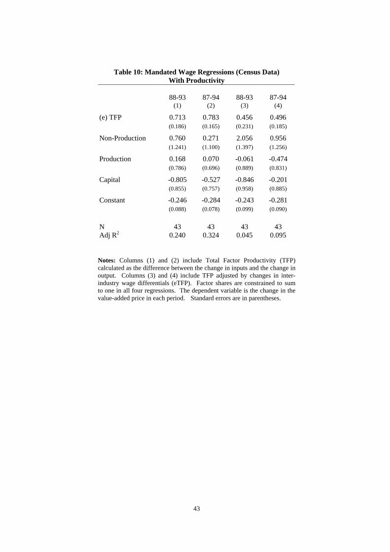
43

Table 10: Mandated Wage Regressions (Census Data)With Productivity

88-93 87-94 88-93 87-94(1) (2) (3) (4)

(e) TFP 0.713 0.783 0.456 0.496(0.186) (0.165) (0.231) (0.185)

Non-Production 0.760 0.271 2.056 0.956(1.241) (1.100) (1.397) (1.256)

Production 0.168 0.070 -0.061 -0.474(0.786) (0.696) (0.889) (0.831)

Capital -0.805 -0.527 -0.846 -0.201(0.855) (0.757) (0.958) (0.885)

Constant -0.246 -0.284 -0.243 -0.281(0.088) (0.078) (0.099) (0.090)

N 43 43 43 43Adj R2 0.240 0.324 0.045 0.095

Notes: Columns (1) and (2) include Total Factor Productivity (TFP)calculated as the difference between the change in inputs and the change inoutput. Columns (3) and (4) include TFP adjusted by changes in inter-industry wage differentials (eTFP). Factor shares are constrained to sumto one in all four regressions. The dependent variable is the change in thevalue-added price in each period. Standard errors are in parentheses.