ROSS SCHOOL OF BUSINESS

CAN PRIVATE WATER COMPANIES DELIVER QUALITY?:

THE ROLE OF SCALE AND CUSTOMER ATTENTIVENESS

Thomas P. Lyon

†, A. Wren Montgomery

‡, and Dan Zhao

§

January 13, 2015

We compare the performance of private versus public water systems in terms of their compliance

with water quality and treatment technique standards. We present a simple theoretical model of

multi-task effort allocation by firms under alternative ownership structures. Our dataset covers

52,011 municipal water systems in the U.S., with more than 200,000 observations over the

period 2010-2013. Empirical estimation is conducted using a number of different specifications

of violations by private and public water systems. Private systems are found to underperform

public systems both in terms of procedural and outcome compliance, with private systems

performing particularly poorly in procedural compliance. Performance effects are moderated by

system size, however. Private systems’ likelihood of being in compliance on outcomes and on

procedures improves with size, and may outperform public systems at large scale.

†Dow Professor, Ross School of Business and School of Natural Resources and Environment, University of

Michigan. tplyon@umich.edu ‡School of Business, Queen’s University, Kingston, Ontario. WMontgomery@business.queensu.ca

§Ross School of Business, University of Michigan. danzhao@umich.edu

Abstract

1

I. INTRODUCTION

Businesses and industry associations around the globe are recognizing the fundamental

challenges that growing pressures on water resources present (2030 Water Resource Group, 2009;

CDP and Deloitte, 2011; KPMG, 2012). Yet, despite this growing attention, management

scholarship has lagged behind in studying the business implications of a water-constrained world,

and the stakeholder and institutional forces that businesses face around water (Kurland & Zell,

2010). Moreover, there is little research exploring how alternative approaches to managing

water, e.g. public vs. private ownership, perform. The need to understand these alternatives is

especially urgent in light of recent conflicts over water in Detroit and Ireland. In the summer and

fall of 2014, protests erupted in Detroit over the 30,000 household water shutoffs by the city’s

water department, with banners and chants repeating“Who’s Water? Our Water” and “Who’s on

our side? United Nations. Who’s on their side? Corporations.”1

Whether crucial social systems such as education, electricity, natural gas, health care,

telecommunications, and water---which are fundamental to our quality of life or even to life

itself---should be provided by public or private entities has long been an issue of heated debate,

and there has been plentiful research on this topic. Masten (2010) points out that water and

sewage systems constitute an anomaly, in that they have traditionally been publicly owned while

other utilities have long been privatized. Water supply has emerged into the spotlight in recent

years following the economic crisis as many municipal governments, especially in the Rust Belt,

considered selling off their water systems to cope with fiscal challenges (Food & Water Watch,

2010).

Privatization advocates argue that market forces provide discipline that leads to lower

costs and more efficient service. However, water privatization often faces strong popular

1 From the authors’ own field observations and data collection.

2

opposition from groups worried that privatization amounts to a very expensive loan that will

result in higher water rates and lower quality of service (Bakker, 2010). The controversy

surrounding Detroit’s water shutoffs in 2014 is but one facet of these political battles.2 In

England, Ireland, and Wales, when Thatcher’s government privatized the 10 regional water

authorities in 1989, similar controversies arose and the results have been decidedly mixed. For

example, Saal & Parker (2000) find that the privatization produced no measurable efficiency

improvements.

Most of the existing literature on privatization has taken a cost-benefit perspective

focusing on cost, pricing and efficiency. Scant attention has been paid to the issue of quality of

service, in particular, compliance with quality standards among water systems of different

ownership statuses. In this paper we aim to fill that gap by studying the relative performance of

public and private water systems with respect to violations of EPA’s Safe Drinking Water Act

(SDWA). We develop a simple model inspired by the economics, finance, and strategy

literatures to explain the effect of privatization, taking into account government monitoring

behavior and the presence of consumers with limited attention. We then use data taken primarily

from EPA’s Safe Drinking Water Information System (SDWIS) to identify the relationship

between different kinds of SDWA violations and ownership statuses, size, and a series of other

factors. Our findings suggest that private systems generally perform more poorly than public

systems, both in terms of pollution outcomes and, even more markedly, procedural compliance

with regulation, but that this underperformance gradually disappears with scale.

The remainder of the paper is structured as follows: Section II reviews the existing

literature on privatization. Section III presents background information on water systems and

2 News link: The Guardian: “Detroit's Water War: a tap shut-off that could impact 300,000 people” Jun 25, 2014

http://www.theguardian.com/environment/true-north/2014/jun/25/detroits-water-war-a-tap-shut-off-that-could-

impact-300000-people

3

their monitoring. Section IV lays out a simple theoretical model and derives several testable

predictions. Section V describes our data sources and presents summary statistics. Section VI

reports empirical specifications and regression results, and Section VII concludes.

I. LITERATURE REVIEW

There is a large literature comparing the merits of public and private ownership. The

findings indicate that there is no universal domination of one mode of governance over the other;

instead, relative performance depends upon a variety of factors such as the complexity of the

technology involved, the predictability of the institutional environment, and the relationship

between cost and quality.

Theoretical work has come from both transaction cost analysis and formal agency theory.

For example, Crocker & Masten (1996) apply a transaction cost approach, starting from the

observation that when relationship-specific investments play a crucial role, the potential for

opportunism may lead to traditional spot markets (which in our case represents private water

systems) being replaced in favor of more structured governance alternatives. When it comes to a

simple market context, the parties may formally assign responsibilities at the very beginning,

creating a long-term relationship administered through contracts. With the complexity of the

market background growing or the cost of negotiation of future duties accumulating, the parties

may choose to implement the exchange through internal administration (public water systems).

Hart, Shleifer & Vishny (1997) derive complementary results using a formal model of

incomplete contracting. They show that public ownership should be preferred when cost

reductions, which are not contractible, may undermine quality to a large extent, when not much

emphasis is needed on quality innovations, and when government procurement suffers from

4

severe corruption. On the contrary, private firms provide a better trade-off when the utilization of

contracts or competition can limit the reduction in quality associated with cost reductions, when

a lot of weight is put on quality innovations, and when the government has a lot of trouble

dealing with patronage and powerful unions.

Within the empirical literature, the bulk of the work has focused on the relative efficiency

of the two alternative governance structures. Megginson and Netter (2001) offer an extensive

review of the empirical literature on privatization. They focus on the methodology and results of

ten prominent recent empirical papers, among which nine find that private enterprises

outperform public ones, while the remaining one finds no significant difference. However, the

authors note that privatization is likely to perform less well in the presence of serious market

failures, and they do not separate out the results for transition economies from results for

developed capitalist economies, nor do they treat separately the privatization of traditionally

monopolistic firms such as public utilities. Thus it is important to delve more deeply into works

that focus on utilities such as electricity, natural gas, telecommunications, and water and sewage.

The 1990 privatization and liberalization of the British electricity industry is assessed by

Newbery and Pollitt (1997), who find significant post-privatization performance improvements.

However, they find that almost all of the financial rewards of this improvement were captured by

the producers and their shareholders, whereas little benefit went to the government or consumers.

Using U.S. data, Koh, Berg, & Kenny (1996) find that municipally owned power plants are more

efficient when output is low, probably due to the more effective public cost control generated by

higher voter attention when jurisdictions are small. Kwoka (2002, 2005) finds that even though

privately-owned electric utilities have an overall cost advantage, publicly-owned utilities offer

significantly lower prices, in part because they perform better in the end-user-oriented

5

distribution function due to quality attributes that are difficult to contract for. Kwoka (2008)

reviews ten studies of the restructuring and privatization of the U.S. electric power industry,

eight of which give electricity restructuring a generally positive appraisal, though most of these

had one or more serious methodological limitations.

A large empirical literature also focuses specifically on water and sewage. Masten (2010)

points out that water and sewage are the only public utilities that are predominantly public in the

U.S. He lays out several possible causes of the historical municipalization of water, and assesses

them using data from the turn of the 19th

century. He finds that the simplicity of early water

supply systems made them less vulnerable to poor management by government bureaucrats, and

that the contentiousness of any attempts to raise water prices made private ownership less

attractive. Troesken & Geddes (2003) use a dataset on municipalization of private water

companies from 1897 to 1915 to support a transaction cost theory for public acquisition. They

conclude that since governments cannot credibly commit to eschew opportunistic expropriation

from the private companies once they have made investments, private companies have weak

incentives to make investments and governments accordingly may need to acquire private water

systems in order to induce appropriate investments.

As for the consequences of water privatization, Bel & Warner (2008) conduct a review of

all published econometric studies of water and waste production since 1970. They do not find

much backing for a connection between privatization and cost savings. For example, no evidence

of cost savings exists in water delivery, and savings are not systematic in waste. In line with this,

Hunt & Lynk (1995) find that the privatization of the UK water industry resulted in significant

efficiency losses due to lost economies of scope. In a rare study of the impact of privatization on

service quality, Troesken (2001) finds African Americans to be a major beneficiary of water

6

municipalization, for it decreases the spread of waterborne-disease among them, however the

effect is much smaller on whites, i.e. public water companies provided blacks with better service

than did private water companies.

Finally, another stream of literature that relates to our study involves the impact of

information on the provision of product quality. Bennear & Olmstead (2008) study the 1996

Amendments to the SDWA, which stipulates that water systems issue annual consumer

confidence reports (CCRs) to their customers and that systems serving over 10,000 people mail

the reports directly to consumers. They conclude that the requirement to mail the CCRs directly

to households significantly decreased violations by water suppliers in Massachusetts. To the

contrary, Johnson (2003) uses an experiment in which customers read different versions of a

water quality report (Consumer Confidence Report) to show that, in contrast to what might be

hoped or feared, the content of the reports per se probably makes little difference to the

consumers.. This finding suggests that consumers of water are not always paying attention to

water quality, even when information is provided directly to them. Together, these papers show

the importance of consumer attention to water quality information, a factor that plays an

important role in our theoretical model.

Overall, the existing literature suggests that privatization may have important impacts on

costs, productivity, prices, and quality. These impacts, however, may depend in subtle ways on

details of the empirical setting, such as scale of operation and demographic factors such as race

or consumer attention to service quality. The effects of private ownership on service quality, in

particular, have received very little empirical attention.

II. BACKGROUND ON WATER SYSTEMS AND THEIR MONITORING

7

A. Overview

According to EPA’s 2012 National Public Water Systems Compliance Report, by the end

of December 2012 there were 150,848 active water systems in the U.S., serving over 320 million

consumers. Among these systems, the vast majority are small systems serving fewer than 10,000

customers. The number of systems with violations decreased from 37,631 in 2011 to 36,536 in

2012. Agencies with enforcement authority, such as state governments, reported that roughly 24

percent of all systems in the U.S. had at least one significant violation in 2012; 6 percent of all

systems in the U.S., serving approximately 23.7 million consumers, had violations of health-

based standards, while monitoring and reporting violations made up another 15 percent. In the

same year, 7,809 enforcement actions were initiated in response to drinking water violations at

water systems. The following graph is from EPA’s 2012 National Public Water Systems (PWSs)

Compliance Report.3

Figure 1

B. Water Supply Models – A Public to Private Continuum

Considering the existence of a range of forms of water system management that entail

both public and private participation, it is a simplification to see water supply models in terms of 3 Note that here “public” means serving the public, not publicly owned.

8

a strict dichotomy between public and private. In practice, there is actually a continuum with

purely public on one end and purely private on the other.

Bakker (2003) characterizes these supply models broadly into 3 categories, providing a

useful framework for our discussion. First is the “public utility” municipal model. This was the

dominant form of water provision over the past century. As the name indicates, the systems are

owned and primarily operated by governments. They are generally not-for-profit, and often have

subsidized rates. The second category is the private sector “commercial” model, under which

systems are managed and sometimes owned by private parties. Popular types in this category

include Private Sector Participation (PSP, also termed Public Private Partnerships) having private

companies managing infrastructures usually owned by municipal governments and it has been

gaining popularity in recent years. Private systems are typically for-profit and have a market-

oriented pricing scheme. The third model, lying somewhere between the aforementioned two, is

the community ‘cooperative’ model. According to Bakker, a cooperative can be defined as “an

enterprise owned and democratically controlled by the users of the goods and services provided.”

This model is more prevalent in rural areas. According to EPA’s Safe Drinking Water

Information System, in Fiscal Year 2013, there are 1322 Community Water Systems serving

4,736,882 residents. Of these, 1135 are small or very small (less than 3300 people), and only 7

serve more than 100,000 residents.

Despite (or perhaps because of) the complexities pointed out above, the EPA, in its Safe

Drinking Water Information System, categorizes each water system as either public or private,

and we will make use of this categorization in the empirical analysis below.

C. Monitoring Process

9

The monitoring process is based upon the Safe Drinking Water Act (SDWA), the primary

federal law to ensure the quality of Americans' drinking water. Originally passed by Congress in

1974 to protect public health by regulating the nation's public drinking water supply, the law

later was amended in 1986 and 1996 and requires many actions to protect drinking water and its

sources: rivers, lakes, reservoirs, springs, and ground water wells.

The Act requires U.S. EPA to set drinking water standards that public water systems

(PWS) (meaning providing drinking water to the public instead of publicly owned) must meet.

US EPA has set standards for 90 contaminants. Under SDWA, states that meet certain

requirements, including setting regulations that are at least as stringent as US EPA’s, may apply

for, and receive primary enforcement authority, or primacy. Individual water systems submit

samples of their water for laboratory testing to verify that the water they provide to the public

meets all federal and state standards. How often and where samples are taken varies according to

numerous conditions. Monitoring schedules differ according to the type of contaminant, the type

of source water used to produce drinking water, and the population served by the public water

system. Each regulation outlines the requirements that systems must follow. US EPA regulations

specify the methods that must be used to analyze drinking water samples. States or the US EPA

certify the laboratories that conduct the analyses.

The SDWA provides states or EPA the authority to grant “variances” that allow public water

systems to use less costly technology, and exemptions to allow public water systems more time

to comply with a new drinking water regulation. Variances allow eligible systems to provide

drinking water that does not comply with a National Primary Drinking Water Regulation

(NPDWR) on the conditions that the system installs a certain technology and that the quality of

the drinking water is still protective of public health. Likewise, exemptions allow eligible

10

systems additional time to build capacity in order to achieve and maintain regulatory compliance

with newly promulgated NPDWRs, while continuing to provide acceptable levels of public

health protection. Exemptions do not release a water system from complying with NPDWRs;

rather, they allow water systems additional time to comply with NPDWRs.

In addition to monitoring methods and frequency, EPA requires community water

systems to deliver annual drinking water quality reports (Consumer Confidence Report) to their

customers. This information supplements public notification that water systems must provide to

their customers upon discovering any violation of a contaminant standard. Large water systems

with more than 10,000 customers must deliver the water quality reports to their customers, and

take steps to get the information to people who do not receive water bills. Water systems serving

fewer than 10,000 people, on the other hand, may be able to distribute the information through

newspapers or by other means. The largest water systems must post their reports on the Internet,

in addition to other delivery mechanisms, to make the reports easily accessible to all consumers.

D. Violations

Violations are detected by assessment of the above-mentioned sample results or reviews

(including on-site visits). Once detected, violations may lead to legal actions or compliance

orders. They will also be publicized, when required, by public notification. Violations may be

remedied by compliance/ enforcement actions, such as improved filtration techniques or changes

in procedures. Some examples of violations include: Maximum Contaminant Level (MCL)

violations, Treatment Technique (TT) violations, failure to replace lead service lines, monitoring

and reporting violations, and procedural violations. Among these, MCL and TT violations are the

two major types of violations that deserve special notice. They themselves also include a

11

multitude of subcategories of violations and they are what we will be looking at primarily in this

paper. An MCL denotes the highest level of a contaminant that EPA allows in drinking water so

as not to pose either a short-term or long-term health risk. EPA sets MCLs at levels that are

economically and technologically feasible. A TT refers to a required process intended to reduce

the level of a contaminant in drinking water. In the table below we list the key types of violations.

Table 1

Key Types of Violations

Abbreviations Full Name

Arsenic Arsenic

CCR Consumer Confidence Report Rule

FBRR Filter Backwash Recycle Rule

GWR Ground Water Rule

I_LT1_ESWTR

Interim Enhanced Surface Water Treatment Rule and the LT1 (future)

Enhanced SWTR

LCR Lead and Copper Rule

LT2_ESWTR LT2 (future) Enhanced SWTR

Misc Miscellaneous

Nitrates Nitrates

Other_IOC Other Inorganic Chemicals

PN_rule Public Notification Rule

Rads Radionuclides

SOC Synthetic Organic Chemicals

St1_DBP Stage 1 Disinfectants By-Product Rule

St2_DBP Stage 2 Disinfectants By-Product Rule

SWTR Surface Water Treatment Rule

TCR Total Coliform Rule

TTHM_pre-St1 TTHM Rule violations, which was replaced by the ST1 DBP Rule

VOC Other Volatile Organic Chemicals

12

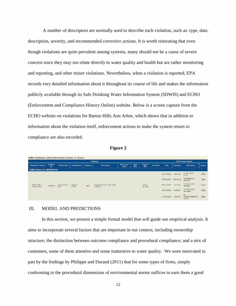
A number of descriptors are normally used to describe each violation, such as: type, date,

description, severity, and recommended corrective actions. It is worth reiterating that even

though violations are quite prevalent among systems, many should not be a cause of severe

concern since they may not relate directly to water quality and health but are rather monitoring

and reporting, and other minor violations. Nevertheless, when a violation is reported, EPA

records very detailed information about it throughout its course of life and makes the information

publicly available through its Safe Drinking Water Information System (SDWIS) and ECHO

(Enforcement and Compliance History Online) website. Below is a screen capture from the

ECHO website on violations for Barton Hills Ann Arbor, which shows that in addition to

information about the violation itself, enforcement actions to make the system return to

compliance are also recorded.

Figure 2

III. MODEL AND PREDICTIONS

In this section, we present a simple formal model that will guide our empirical analysis. It

aims to incorporate several factors that are important in our context, including ownership

structure; the distinction between outcome compliance and procedural compliance; and a mix of

customers, some of them attentive and some inattentive to water quality. We were motivated in

part by the findings by Philippe and Durand (2011) that for some types of firms, simply

conforming to the procedural dimensions of environmental norms suffices to earn them a good

13

reputation, but firms in environmentally sensitive industries must conform to both procedural

and goal dimensions of the norms in order to earn a good reputation, because they are subject to

more stringent public monitoring. Our formal modeling approach was motivated in part by the

work of Hart, Shleifer & Vishny (1997), which showed that privately-owned systems may be

able to achieve lower costs but may provide either higher or lower quality compared with public

systems. However our model differs in several important ways from theirs. In particular, we

include the possibility of monitoring by both government and consumers, the possibility that

only a fraction of consumers are attentive to issues of water quality, and the possibility of

compliance with both procedural and outcome requirements.

We assume there are two kinds of effort that a water system can devote to its level of

compliance:

t = effort towards procedural compliance

m = effort towards outcome compliance

These efforts have effects on compliance levels characterized by two dimensions:

outcome compliance level (M), a failure of which is reflected by Maximum Contaminant Level

(MCL) violations, and procedural compliance level (T), a failure of which is reflected by

Treatment Technique (TT) violations:

𝑀(𝑚) = 2𝑚12

𝑇(𝑡) = 2𝑡12

Our use of specific functional forms allows us to obtain closed-form solutions but without any

meaningful loss of generality in our hypotheses, which would remain directionally unchanged

for any concave functions ( 𝑀′(𝑚) > 0, 𝑇′(𝑡) > 0, 𝑀′′(𝑚) < 0, 𝑇′′(𝑡) < 0).

14

Of course these efforts dedicated to compliance come at a cost. Letting s denote the size

of the system, we represent the system’s costs as

𝐶(𝑡, 𝑚, 𝑠) = 𝐶0 +𝜌

𝑠𝑡

23 +

𝛾

𝑠𝑚

23

We assume the cost function 𝐶(𝑡, 𝑚, 𝑠) to be concave due to economies of scale. Here 1

𝑆

implies that the bigger the size of the system, the more efficient it becomes in applying

compliance effort. Again, our use of specific functional forms is just a particular concave

functional form that is adopted for simplicity in obtaining closed-form solutions.

The system’s compliance levels determine the government monitoring agency’s (EPA’s)

assessments of the systems. Let A denote EPA’s assessment of a water system’s compliance

level, which we will assume takes the additive form:

𝐴(𝑀, 𝑇) = 𝛼𝑀(𝑚) + 𝛽𝑇(𝑡).

This specification captures the notion that government bureaucrats assess the performance of

water systems by assigning weights (𝛼, 𝛽 ∈ 𝑅+) to outcome and procedural compliance levels

respectively, i.e. we define their utility by adding up the weighted compliance levels.

Not only will the system’s compliance level determine the government’s assessment,

compliance will also define the water system’s reputation among consumers, investors and the

general public. Focusing on consumers, we assume, following previous work in finance and

accounting (Hirshleifer & Teoh, 2003; Bagnoli & Watts, 2014) that they have limited attention

and information processing power. On this ground we can differentiate between two kinds of

consumers: 1) attentive, relatively rational, Bayesian individuals, and 2) inattentive individuals

who use simple heuristics in their decision making. More specifically, we assume that for every

system, a proportion 𝑝 ∈ [0,1] of its consumers are attentive, and 1-p are not.

15

Finally, we also draw from the law and economics literature on accidents and optimal

precaution, and assume that for a certain level of outcome compliance, there exists some chance

a(M) that a water quality accident leading to a public health incident will occur (Shavell, 1984;

Kolstad et al., 1990). We assume a’(M)= k < 0. We assume 𝑘, the derivative of the 𝑎(𝑀)

function, to be an unknown constant illustrating the notion that the exact extent to which changes

in compliance level affect occurrence of accidents is unknown to any parties. If such an incident

occurs, some harm H will be done to the water system’s customers and also to its reputation (or

there may be more direct punishments to the system). We assume 𝐻 to be an increasing function

of 𝑠, the size of the system represented by the population served, to convey the notion that the

bigger a system is, the more severe the damage may be. We let H(s) = ℎs for simplicity.

Letting R stand for the water system’s reputation in the eyes of consumers, we have:

𝑅(𝑝, 𝑀, 𝑇, 𝑠) = 𝑝𝐴(𝑀, 𝑇) + (1 − 𝑝)[𝛿𝜔𝑀(𝑚)] − 𝐻(𝑠)𝑎(𝑀). (1)

The first term on the right-hand side of this expression reflects the evaluations of

attentive consumers, who read the annual Consumer Confidence Reports, check the EPA website,

and may even go and visit the water plants in person; they are assumed to completely observe the

reported compliance levels, just like government officials do. They also evaluate the system’s

reputation in the same manner government bureaucrats assess the water system.

The second term in equation (1) reflects the role of inattentive consumers, who typically

do not raise any concern about how their drinking water is processed and only become informed

when a public notification is issued. Our representation of inattentive consumers makes use of an

interesting pattern in the distribution of enforcement action types for MCL and TT violations. In

our data, around 50 percent of MCL violations have public notifications issued, while only

around 23 percent of TT violations ever have public notifications issued. A bold simplification is

16

made in our model that inattentive customers only pay attention to public notifications about

MCL violations, i.e. outcome compliance. This reflects both the greater likelihood of MCL

violations been announced publicly, as well as the greater import of MCL violations for

customer health. Furthermore, the outcome compliance level they observe (that is, the

proportion of MCL violations) is characterized by 𝜔 < 1. After they observe the outcome

compliance level, they assign weight 𝛿 to this information. We assume that 𝛿 < 𝛼, the weighting

parameter used by bureaucrats and attentive customers, since the inattentive consumers probably

won’t take the observed information as seriously as the bureaucrats or attentive consumers do.

The third term in equation (1) captures the risk of harm due to lack of effort on the

system’s part. It is assumed that both the attentive and inattentive consumers downgrade the

system’s reputation when public health incidents arise. The way inattentive consumers are

modelled reflects the idea that inattentive consumers are not totally passive and will partially

observe compliance levels when that information is specifically brought forward to them, and

punish the water system when a severe accident does occur.

The proportion of attentive consumers, p, can be thought of as a function of two variables.

One is the level of local educational attainment. As people become better educated, they tend to

care more about their health and quality of life, and thus the quality of the water they drink.

Similarly, the poverty rate can also play a role. As more residents fall below the poverty line,

fewer of them are inclined to pay attention to their water quality, since they have more urgent

matters to attend to. (The poverty rate may also influence the compliance level indirectly

through the financial conditions of the municipal governments and thus funding in maintaining

17

and upgrading the equipment of the water systems.)4 Letting 𝐸 denote educational attainment

and 𝑃 the poverty rate, mathematically we can write:

𝑝 = 𝑝(𝐸, 𝑃),

with

𝜕𝑝

𝜕𝐸> 0,

𝜕𝑝

𝜕𝑃< 0.

Combining the foregoing model elements, we characterize the water system’s total utility

as a function of the government’s assessment of its performance, its reputation, and its costs. We

let 𝜆(𝑂) ∈ [0,1] represent the relative weight given to the government’s assessment, which we

assume is a function of the ownership status O of the system. We assume O to be a continuous

variable which takes the value of 0 when a system is completely public and 1 when the system is

completely private. This takes into consideration the fact that the notion of a simple dichotomy

of ownership status is a simplification, and we can actually view the water systems’ ownership

status as ranging from absolute public to public/private cooperation to absolute private

ownership. This representation reflects the notion that the publicly owned systems who answer

to bureaucrats likely have limited incentive to respond to public opinion on their performance.

As for private systems, even though they are also subject to some bureaucratic regulation, they

also place substantial weight on their public reputation, especially since for-profit provision of

water is often viewed with suspicion by the public and water privatization has been a topic of

public debate in recent years. So 𝜆 is close to 1 when the system is public and close to 0 when

the system is private, with 𝜕𝜆

𝜕𝑂< 0.

Thus, we can ultimately write the system’s total utility U as:

4 If we consider 𝑝 from the viewpoint of a water system, we might also hypothesize that as the system size increases,

the water system has a “stronger presence” in town and draws more attention from the public, so 𝑝 for its pool of

consumers may increase.

18

𝑈(𝐴, 𝑅, 𝐶, 𝜆) = 𝜆𝐴(𝑀, 𝑇) + (1 − 𝜆)𝑅(𝑝, 𝑀, 𝑇, 𝑠) − 𝐶(𝑡, 𝑚, 𝑠).

Substituting in, we have:

𝑈(𝐴, 𝑅, 𝐶, 𝜆) = 𝜆[𝛼𝑀(𝑚) + 𝛽𝑇(𝑡)] + (1 − 𝜆)[𝑝𝐴(𝑀, 𝑇) + (1 − 𝑝)[𝛿𝜔𝑀(𝑚)] − 𝐻(𝑠)𝑎(𝑀)]

− (𝐶0 +𝜌

𝑠𝑡

23 +

𝛾

𝑠𝑚

23)

or, in terms of the underlying variables,

𝑈(𝑡, 𝑚, 𝜆, 𝑝, 𝑠) = 𝜆 (𝛼2𝑚12 + 𝛽2𝑡

12)

+ (1 − 𝜆) [𝑝 (𝛼2𝑚12 + 𝛽2𝑡

12) + (1 − 𝑝) (𝛿𝜔2𝑚

12) − ℎ𝑠𝑎(𝑀)]

−(𝐶0 +𝜌

𝑠𝑡

23 +

𝛾

𝑠𝑚

23)

Now a water system solves the following maximization problem:

max𝑡,𝑚

{𝜆 (𝛼2𝑚12 + 𝛽2𝑡

12) + (1 − 𝜆) [𝑝 (𝛼2𝑚

12 + 𝛽2𝑡

12) + (1 − 𝑝) (𝛿𝜔2𝑚

12) − ℎ𝑠𝑎(𝑀)] − (𝐶0

+𝜌

𝑠𝑡

23 +

𝛾

𝑠𝑚

23)}

Taking the first-order conditions and solving for the optimal effort levels (𝑚∗, 𝑡∗), we obtain

𝑡∗ =729𝛽6𝑠6(𝑝𝜆 − 𝑝 − 𝜆)6

64𝜌6 (2)

and

𝑚∗ =729𝑠6(ℎ𝑠𝜆𝑘 − ℎ𝑘𝑠 + 𝛼𝑝 − 𝛼𝑝𝜆 + 𝛼𝜆)6

64𝛾6 . (3)

Differentiating these expressions with respect to size and customer attentiveness, we obtain

the following comparative statics results:

𝜕𝑡∗

𝜕𝑠=

2187𝛽6𝑠5(𝑝(𝜆 − 1) − 𝜆)6

32𝜌6> 0

19

𝜕𝑡∗

𝜕𝑝=

2187𝛽6𝑠6(𝜆 − 1)(𝑝(𝜆 − 1) − 𝜆)5

32𝜌6> 0

𝜕𝑚∗

𝜕𝑠=

2187𝑠5(ℎ𝑘𝑠(𝜆 − 1) − 𝛼(𝑝(𝜆 − 1) − 𝜆))5

(2ℎ𝑘𝑠(𝜆 − 1) − 𝛼(𝑝(𝜆 − 1) − 𝜆))

32𝛾6> 0

𝜕𝑚∗

𝜕𝑝= −

2187𝛼𝑠6(𝜆 − 1)(ℎ𝑘𝑠(𝜆 − 1) − 𝛼(𝑝 (𝜆 − 1) − 𝜆))5

32𝛾6> 0.

These results imply that as the size of systems increase, they improve on both procedural

and outcome compliance. In addition, since 𝜕𝑡∗

𝜕𝑝> 0 and

𝜕𝑚∗

𝜕𝑝> 0, and

𝜕𝑝

𝜕𝐸> 0,

𝜕𝑝

𝜕𝑃< 0, the

model predicts that both procedural and outcome compliance are growing as local educational

attainment and poverty conditions improve. Thus, we have the following hypothesis:

Hypothesis 1: Both procedural compliance and outcome compliance are higher for large systems,

and systems serving communities with higher levels of local educational attainment and lower

rates of poverty.

Turning now to our primary interest, the role of ownership status, we find that

𝜕𝑡∗

𝜕𝜆=

2187𝛽6(𝑝 − 1)𝑠6(𝑝(𝜆 − 1) − 𝜆)5

32𝜌6> 0

𝜕𝑚∗

𝜕𝜆=

2187𝑠6(𝛼 + ℎ𝑘𝑠 − 𝛼𝑝)(ℎ𝑘𝑠(𝜆 − 1) + 𝛼(𝑝(−𝜆) + 𝑝 + 𝜆))5

32𝛾6 0.<

>

The first of these expressions shows that publicly-owned systems tend to have higher rates of

procedural compliance, which we state explicitly as

Hypothesis 2: Procedural compliance is higher for publicly-owned water systems.

20

Interestingly, however, unlike our prediction for procedural compliance, the sign of 𝜕𝑚∗

𝜕𝜆

is undetermined in general. When 𝛼(1 − 𝑝) > −ℎ𝑠𝑘, 𝜕𝑚∗

𝜕𝜆> 0, and when 𝛼(1 − 𝑝) < −ℎ𝑠𝑘,

𝜕𝑚∗

𝜕𝜆< 0. Intuitively this means when the proportion of inattentive consumers is high enough and

the size of the system is small enough (such that the product of it and the weight attentive

consumers assign to outcome compliance is larger than the harm of an accident multiplied by the

negative marginal likelihood of an accident), public systems will have a higher outcome

compliance level. On the other hand, when enough consumers are attentive and the water system

is big enough, private systems may outperform public ones in outcome compliance. Thus, we

have our final hypothesis:

Hypothesis 3: Outcome compliance is higher under public ownership for small systems with a

relatively high proportion of inattentive customers. Outcome compliance is higher under private

ownership for large systems with a relatively high proportion of attentive customers.

In sum, the model predicts that private systems underperform public systems in terms of

procedural compliance, but which kind of system has a higher outcome compliance level varies

depending on the proportion of consumers who are attentive to water quality and the size of the

water system. In addition, as the size of water systems increases, they tend to do better both in

terms of procedural and outcome compliance. Finally, both compliance levels are higher for

systems in areas with higher education attainment levels and lower poverty rates.

IV. DATA SOURCES AND SUMMARY STATISTICS

Data Description

21

The primary source of data used in this study is the Environmental Protection Agency’s

official website, and specifically the Government Performance and Results Act (GPRA) pivot

tables in the Drinking Water Data from the Safe Drinking Water Information System Federal

(SDWISFED). The water systems in the datasets are classified into seven ownership categories.

They are: Federal government, State government, Local government, Mixed public/private,

Native American, Private, and not specified. In the regressions we perform in the following

section, we only consider the three government and one private ownership categories, leaving

out the other types in order to sharpen our empirical analysis.

The pivot tables contain data regarding water systems that have reported GPRA

violations. Violations are counted towards GPRA if they are health-based violations at

community water systems that are open5 during the fiscal year (FY) 2010, 2011, 2012, or 2013.

Our unit of observation is a pair: water system ID# - Fiscal Year. The oldest violations that

remained open in our dataset were first reported in fiscal year 1993. Health-based violations

include MCL, MRDL and TT violations. MCL refers to Maximum Contaminant Level while

MRDL and TT refer to Maximum Residual Disinfectant Level and Treatment Technique,

respectively. (No MRDL violations are recorded for the water systems we look at.) For every

violation, additional information is provided including the ID and name of the public water

system it is associated with, which state and county the system is in, its source of water (surface

or ground), its size as measured by population served, the system’s first and last reported date, its

ownership status, the violation’s ID, violation and contaminant type and name, date a violation

was first reported to SDWIS-Fed, its enforcement action date and type, number of system and

5Violations are considered open during (some or all of) FY 2013 if the calendar date of the beginning of a

monitoring period in which a public water system was determined to be in violation of a primary drinking water

regulation is earlier than or equal to 6/30/2013 and the calendar date of the end of a monitoring period in which a

public water system was determined to be in violation of a primary drinking water regulation is later than or equal to

7/1/2012. The same is true for FY 2010 to 2012.

22

population in violation, total number of systems and population, and finally, fiscal year. In

addition to this main data set, the study also uses per capita personal income by county from the

CA1-3 Personal Income Summary in U.S. Bureau of Economic Analysis (BEA) Regional Data,

GDP & Personal Income. Finally, these data sets are supplemented by information from the

Missouri Census Data Center on the percentage of people with a Bachelor’s degree or higher, the

poverty rate, and the unemployment rate at the county level.

A. Summary Statistics

Over the four years 2010-2013, we have data on 52,011 public water systems, with

200,055 water system-FY observations, and 39,386 violation records. Thus, the vast majority of

water systems had zero violations in any given year. The following table presents some basic

statistics about the size of all the systems in the data set by ownership status.

Table 2

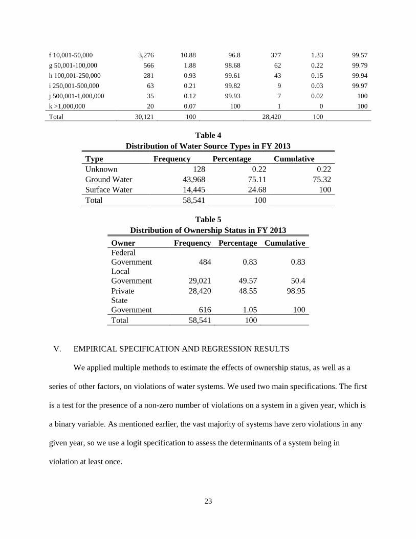
To illustrate the structure of the industry, the distribution of the size categories (retail population

served), the water source type (ground or surface water or unknown) of the water systems, as

well as the ownership status of water systems in fiscal year 2013 are listed below.

Table 3

Distribution of Size Categories in FY 2013

Public Private

Size Categories Frequency Percentage Cumulative Frequency Percentage Cumulative

a <=100 2,021 6.71 6.71 12,692 44.66 44.66

b 101-500 6,907 22.93 29.64 11,267 39.64 84.3

c 501-1,000 4,296 14.26 43.9 1,831 6.44 90.75

d 1,001-3,300 7,647 25.39 69.29 1,576 5.55 96.29

e 3,301-10,000 5,009 16.63 85.92 555 1.95 98.24

23

f 10,001-50,000 3,276 10.88 96.8 377 1.33 99.57

g 50,001-100,000 566 1.88 98.68 62 0.22 99.79

h 100,001-250,000 281 0.93 99.61 43 0.15 99.94

i 250,001-500,000 63 0.21 99.82 9 0.03 99.97

j 500,001-1,000,000 35 0.12 99.93 7 0.02 100

k >1,000,000 20 0.07 100 1 0 100

Total 30,121 100 28,420 100

Table 4

Distribution of Water Source Types in FY 2013

Type Frequency Percentage Cumulative

Unknown 128 0.22 0.22

Ground Water 43,968 75.11 75.32

Surface Water 14,445 24.68 100

Total 58,541 100

Table 5

Distribution of Ownership Status in FY 2013

Owner Frequency Percentage Cumulative

Federal

Government 484 0.83 0.83

Local

Government 29,021 49.57 50.4

Private 28,420 48.55 98.95

State

Government 616 1.05 100

Total 58,541 100

V. EMPIRICAL SPECIFICATION AND REGRESSION RESULTS

We applied multiple methods to estimate the effects of ownership status, as well as a

series of other factors, on violations of water systems. We used two main specifications. The first

is a test for the presence of a non-zero number of violations on a system in a given year, which is

a binary variable. As mentioned earlier, the vast majority of systems have zero violations in any

given year, so we use a logit specification to assess the determinants of a system being in

violation at least once.

24

Our second specification probes more deeply into variation amongst violating firms,

using as a dependent variable total violation duration per system, which involves adding up the

duration of all violations associated with a water system in each year. We define the violation

duration as the year compliance period ended6 minus the first year a violation was reported + 1.

This variable is intended to capture both the number and the duration of violations at a water

system, and serves as a composite estimate of occurrence of violations. A histogram of this

variable is presented in Figure 3. See appendix A for histograms of MCL and TT violation

durations.

Figure 3

Each of these approaches is applied separately to total violations of all types, Maximum

Contaminant Level (MCL) violations, and Treatment Technique (TT) violations. Our basic

specification is as follows, where subscripts it denotes water system i’s record in fiscal year t,

since our unit of observation is water system – fiscal year.

6 This refers to the end of a monitoring period in which a public water system was determined to be in violation of a

primary drinking water regulation

25

𝑉𝑖𝑜𝑙𝑎𝑡𝑖𝑜𝑛𝑠𝑖𝑡 = 𝛽0 + 𝛽1𝑃𝑟𝑖𝑣𝑎𝑡𝑒 𝑆𝑦𝑠𝑡𝑒𝑚𝑖𝑡 + 𝛽2𝑅𝑒𝑡𝑎𝑖𝑙 𝑃𝑜𝑝𝑢𝑙𝑎𝑡𝑖𝑜𝑛 𝑆𝑒𝑟𝑣𝑒𝑑𝑖𝑡

+ 𝛽3𝑈𝑠𝑒𝑠 𝐺𝑟𝑜𝑢𝑛𝑑 𝑊𝑎𝑡𝑒𝑟𝑖𝑡 + 𝛽4𝑂𝑙𝑑 𝑆𝑦𝑠𝑡𝑒𝑚𝑖𝑡 + 𝛽5𝑃𝑒𝑟 𝐶𝑎𝑝𝑖𝑡𝑎 𝐼𝑛𝑐𝑜𝑚𝑒𝑖𝑡

+ 𝛽5𝑈𝑛𝑒𝑚𝑝𝑙𝑜𝑦𝑚𝑒𝑛𝑡 𝑅𝑎𝑡𝑒𝑖𝑡 + 𝛽6𝑃𝑜𝑣𝑒𝑟𝑡𝑦 𝑅𝑎𝑡𝑒𝑖𝑡

+ 𝛽7𝐸𝑑𝑢𝑐𝑎𝑡𝑖𝑜𝑛𝑎𝑙 𝐴𝑡𝑡𝑎𝑖𝑛𝑚𝑒𝑛𝑡𝑖𝑡

+ 𝛽8𝑃𝑟𝑖𝑣𝑎𝑡𝑒 𝑆𝑦𝑠𝑡𝑒𝑚 × 𝑅𝑒𝑡𝑎𝑖𝑙 𝑃𝑜𝑝𝑢𝑙𝑎𝑡𝑖𝑜𝑛 𝑆𝑒𝑟𝑣𝑒𝑑𝑖𝑡 + 𝑆𝑡𝑎𝑡𝑒 𝐼𝑛𝑑𝑖𝑐𝑎𝑡𝑜𝑟𝑠𝑖𝑡

+ 휀𝑖𝑡

We thus regress our dependent variables on the indicator variable for whether the system

is private or not, along with a series of control variables including: its size characterized as

average daily population served at a water system; whether its primary source of water is

groundwater or surface water; whether the system is considered old (33 years or older)7; per

capita income in the county; percentage of unemployed residents in the county; poverty rate in

the county; and percentage of people with Bachelor’s degree or higher in the county. We also

include state dummies to control for state fixed effects. Lastly we include an interaction term

between ownership status and size in order to test our Hypothesis 3.

Table 6 presents a correlation matrix for our four county-level control variables.

Table 6

Correlation Matrix

(obs=185735)

Per Capita

Income

Unemployment

Rate

Educational

Attainment

Poverty

Rate

Per Capita Income 1

Unemployment Rate -0.4269 1

Educational Attainment 0.6738 -0.308 1

Poverty Rate -0.6201 0.5439 -0.4811 1

7 There is a reason for using this indicator variable for old instead of reported age. Since a lot of systems have been

established for a long time but only started reporting to the EPA when the Safe Drinking Water Information System

began to collect their information back in the 70s, their reported age may not necessarily be their real age, which can

be much longer. Using a cutoff point of 33 years to generate the dummy simplifies the problem.

26

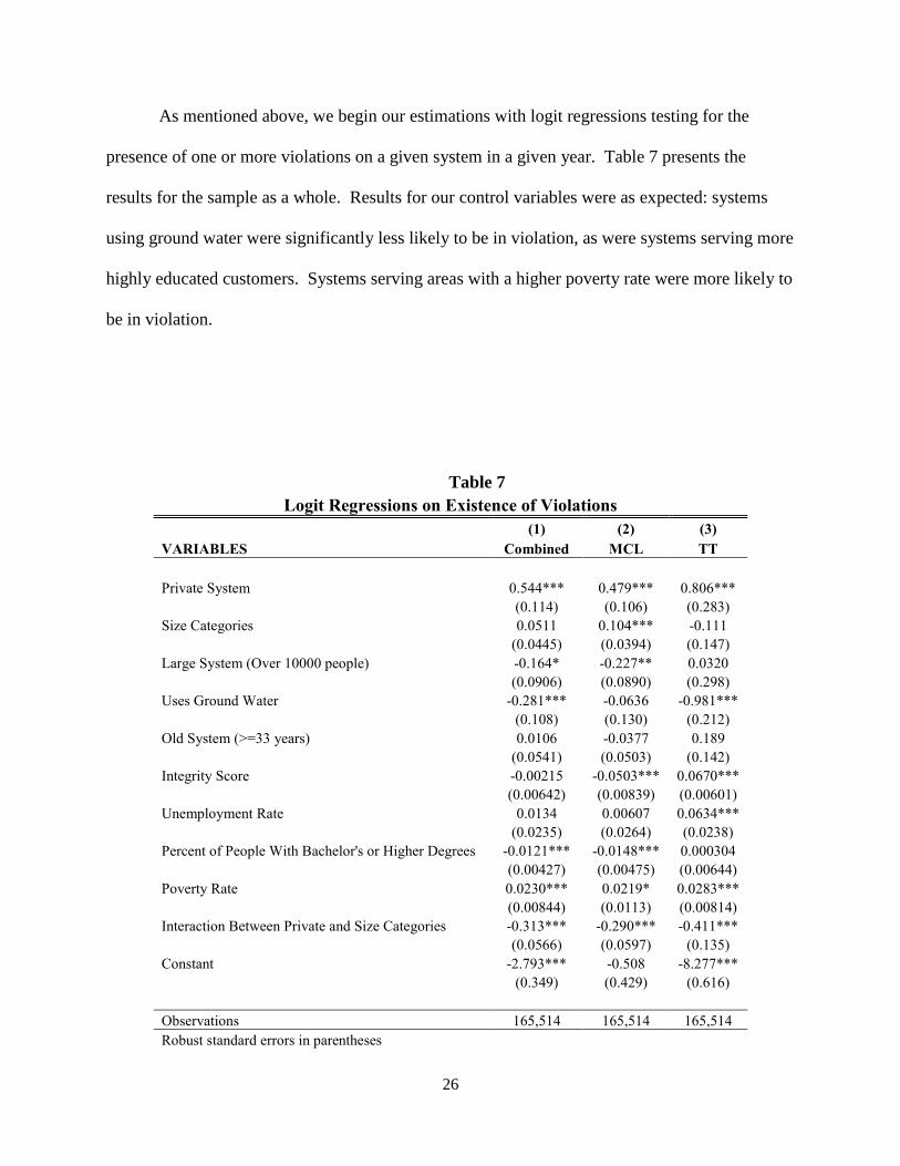
As mentioned above, we begin our estimations with logit regressions testing for the

presence of one or more violations on a given system in a given year. Table 7 presents the

results for the sample as a whole. Results for our control variables were as expected: systems

using ground water were significantly less likely to be in violation, as were systems serving more

highly educated customers. Systems serving areas with a higher poverty rate were more likely to

be in violation.

Table 7

Logit Regressions on Existence of Violations

(1) (2) (3)

VARIABLES Combined MCL TT

Private System 0.544*** 0.479*** 0.806***

(0.114) (0.106) (0.283)

Size Categories 0.0511 0.104*** -0.111

(0.0445) (0.0394) (0.147)

Large System (Over 10000 people) -0.164* -0.227** 0.0320

(0.0906) (0.0890) (0.298)

Uses Ground Water -0.281*** -0.0636 -0.981***

(0.108) (0.130) (0.212)

Old System (>=33 years) 0.0106 -0.0377 0.189

(0.0541) (0.0503) (0.142)

Integrity Score -0.00215 -0.0503*** 0.0670***

(0.00642) (0.00839) (0.00601)

Unemployment Rate 0.0134 0.00607 0.0634***

(0.0235) (0.0264) (0.0238)

Percent of People With Bachelor's or Higher Degrees -0.0121*** -0.0148*** 0.000304

(0.00427) (0.00475) (0.00644)

Poverty Rate 0.0230*** 0.0219* 0.0283***

(0.00844) (0.0113) (0.00814)

Interaction Between Private and Size Categories -0.313*** -0.290*** -0.411***

(0.0566) (0.0597) (0.135)

Constant -2.793*** -0.508 -8.277***

(0.349) (0.429) (0.616)

Observations 165,514 165,514 165,514

Robust standard errors in parentheses

27

*** p<0.01, ** p<0.05, * p<0.1

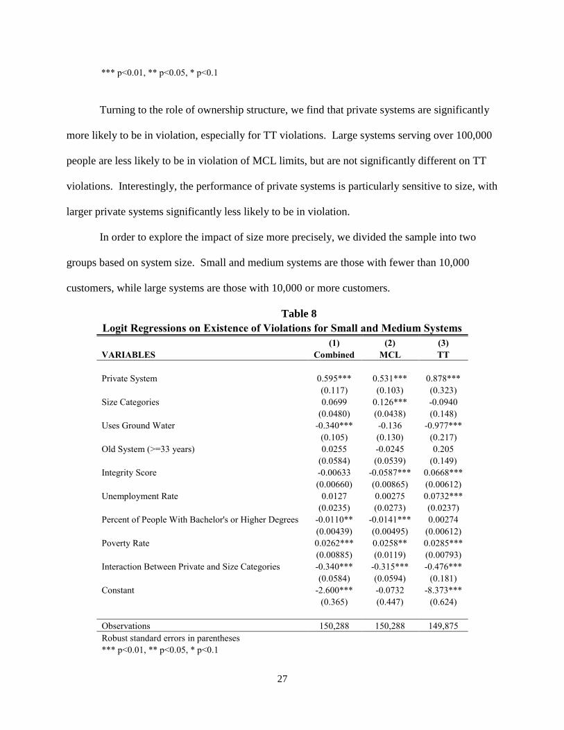
Turning to the role of ownership structure, we find that private systems are significantly

more likely to be in violation, especially for TT violations. Large systems serving over 100,000

people are less likely to be in violation of MCL limits, but are not significantly different on TT

violations. Interestingly, the performance of private systems is particularly sensitive to size, with

larger private systems significantly less likely to be in violation.

In order to explore the impact of size more precisely, we divided the sample into two

groups based on system size. Small and medium systems are those with fewer than 10,000

customers, while large systems are those with 10,000 or more customers.

Table 8

Logit Regressions on Existence of Violations for Small and Medium Systems

(1) (2) (3)

VARIABLES Combined MCL TT

Private System 0.595*** 0.531*** 0.878***

(0.117) (0.103) (0.323)

Size Categories 0.0699 0.126*** -0.0940

(0.0480) (0.0438) (0.148)

Uses Ground Water -0.340*** -0.136 -0.977***

(0.105) (0.130) (0.217)

Old System (>=33 years) 0.0255 -0.0245 0.205

(0.0584) (0.0539) (0.149)

Integrity Score -0.00633 -0.0587*** 0.0668***

(0.00660) (0.00865) (0.00612)

Unemployment Rate 0.0127 0.00275 0.0732***

(0.0235) (0.0273) (0.0237)

Percent of People With Bachelor's or Higher Degrees -0.0110** -0.0141*** 0.00274

(0.00439) (0.00495) (0.00612)

Poverty Rate 0.0262*** 0.0258** 0.0285***

(0.00885) (0.0119) (0.00793)

Interaction Between Private and Size Categories -0.340*** -0.315*** -0.476***

(0.0584) (0.0594) (0.181)

Constant -2.600*** -0.0732 -8.373***

(0.365) (0.447) (0.624)

Observations 150,288 150,288 149,875

Robust standard errors in parentheses

*** p<0.01, ** p<0.05, * p<0.1

28

Table 8 presents the results for small and medium-sized systems. Once again we find

that private systems are significantly more likely to be in violation, both for MCL limits and TT

requirements. And once again, we find that there is an important interaction effect between

ownership status and size, with large private systems performing much better than smaller ones.

Table 9 repeats the estimation for the subsample of large systems. A striking difference

emerges compared to the previous estimates. Private systems are estimated to have fewer

violations than public systems, although the difference is not statistically significant. Large

systems of both types perform better than small systems on MCL violations, but are not

significantly different from small systems on TT violations. In addition, systems serving more

highly educated customers perform better, at least for TT violations.

Table 9

Logit Regressions on Existence of Violations for Large Systems

(1) (2) (3)

VARIABLES Combined MCL TT

Private System -2.313 -2.617 -1.219

(2.286) (2.855) (4.199)

Size Categories -0.681*** -0.866*** -0.278

(0.226) (0.276) (0.320)

Uses Ground Water 0.0171 0.262* -1.275***

(0.151) (0.149) (0.392)

Old System (>=33 years) -0.115 -0.138 0.0139

(0.0828) (0.0916) (0.200)

Integrity Score 0.219*** 0.159*** 0.162***

(0.0453) (0.0499) (0.00864)

Unemployment Rate 0.00827 0.0284 -0.138**

(0.0291) (0.0337) (0.0674)

Percent of People With Bachelor's or Higher Degrees -0.0175** -0.0146 -0.0308**

(0.00786) (0.00905) (0.0145)

Poverty Rate 0.00642 0.000280 0.0458**

(0.0104) (0.0101) (0.0229)

Interaction Between Private and Size Categories 0.415 0.506 0.152

(0.535) (0.685) (0.990)

Constant -14.84*** -10.19*** -10.75***

(3.449) (3.796) (1.750)

29

Observations 14,728 14,688 12,673

Robust standard errors in parentheses

*** p<0.01, ** p<0.05, * p<0.1

Our findings thus far are strongly supportive of our first two hypotheses. As predicted by

Hypothesis 1, larger systems and systems with more attentive customers (as proxied by high

levels of education or low poverty rates) tend to have higher levels of compliance with MCL

outcomes and TT procedures. As predicted by Hypothesis 2, public systems outperform private

ones on procedural compliance, although the evidence for this is less persuasive for large private

firms. Support for Hypothesis 3 is more nuanced. Small and medium-sized private systems

definitely improve more with scale than do public ones, and private systems appear to perform

equivalently to public systems at large scale. However, contrary to Hypothesis 3, we do not

observe private systems actually outperforming public systems, even at scale.

We turn next to our analyses of total violation duration. There are numerous empirical

methods for performing these regressions. The simplest and most familiar is ordinary least

squares, which we include as a reference point. We also run a negative binomial model, as well

as the Tobit model, which takes the zero values for the violations as being censored. However,

considering the large number of observations with zero violations, we also use a zero-inflated

binomial regression (zinb). This is consistent with the fact that the data is over dispersed (i.e.

variance is much larger than the mean). This model deals with the issue of “excess” zeros

because in a zero-inflated model, there are two different processes that generate every

observation. A logit model, like that presented above, is used to determine which of the two

processes is applied. As a result, one process leads to certain zeros while the other process leads

to a count variable which can either be zero or positive. For the count variable, the negative

30

binomial model is used. In our model, the state dummies are used as inflators, considering the

possibility that state fixed effects may be driving the occurrences of zeros.

Table 10 presents the results for our regressions on total violation duration. Once again

we find that private systems perform worse; in this case that means they have more violations of

longer duration, than public systems. Scale economies of performance are again found, with

larger systems having lower violation durations. Systems sourced with ground water perform

better, while old systems perform worse. Systems in areas with high poverty rates or low levels

of education tend to perform worse, though significance varies across different estimating

techniques. The interaction between size and private ownership is not as marked in our violation

regressions, and is only significant for the OLS estimations.

Table 10

Regressions on Total Violation Duration

(1) (2) (3) (4)

VARIABLES

Ordinary

Least

Squares

Negative

Binomial Tobit

Zero-

inflated

Negative

Binomial

Private System 0.136** 0.276*** 1.651*** 0.241**

(0.0535) (0.0902) (0.465) (0.0957)

Retail Population Served -4.57e-07*** -3.67e-06*** -2.40e-05* -2.51e-06*

(1.67e-07) (1.13e-06) (1.35e-05) (1.36e-06)

Uses Ground Water -0.302*** -0.550*** -3.516*** -0.499***

(0.0770) (0.0925) (0.626) (0.0939)

Old System 0.110** 0.221** 1.849*** 0.193**

(0.0440) (0.0871) (0.441) (0.0939)

Per Capita Income 3.46e-06 1.59e-05** 4.98e-05 5.36e-06

(3.60e-06) (6.64e-06) (3.33e-05) (6.05e-06)

Unemployment Rate 0.0120 0.0215 -0.153* 0.0517***

(0.00973) (0.0172) (0.0890) (0.0148)

Poverty Rate 0.00306 0.0431*** 0.306*** -0.0109

(0.00477) (0.00960) (0.0511) (0.00919)

Educational Attainment -0.00600** -0.0116** -0.136*** -0.00315

(0.00243) (0.00593) (0.0303) (0.00524)

Interaction Between Private and Population -7.95e-07* 4.86e-07 1.53e-06 -1.14e-06

(4.77e-07) (2.77e-06) (3.15e-05) (2.44e-06)

Constant 0.812 -2.285*** -29.92*** -0.367

31

(0.536) (0.514) (3.907) (0.343)

Observations 47,101 47,101 47,101 47,101

R-squared 0.011

Robust standard errors in parentheses

*** p<0.01, ** p<0.05, * p<0.1

Overall, we find that private systems perform worse, on both MCL and TT violations, but

private systems do especially badly on TT violations (the magnitudes of the TT coefficients are

generally significantly larger than MCL coefficients, and their significance is higher). Also, as

the size of water systems increases, private systems often improve their performance relative to

public systems; in particular they tend to exceed public systems by a lesser amount in terms of

MCL violations in most cases but the interaction terms often show mixed signs for TT violations

(sometimes there may even be more TT violations as size gets bigger). Furthermore, larger

systems are less likely to have violations, even though sometimes the effect is weak, and the

effect on MCL violations is slightly stronger than that on TT violations.8

The predictions of our model are largely confirmed. In particular, both the model and

empirical results show that private systems underperform public systems in terms of procedural

compliance, but which kind of systems has a higher outcome compliance level is undetermined

in general, since the interaction terms for MCL violations tend to be more significant than those

for TT violations and they have a negative sign. However, even though the model predicts that

this undetermined nature comes from the proportion of attentive consumers and size of the water

system, in the empirics it seems to be size that is primarily driving the variation.

8 We also conducted a number of robustness checks, some of which are presented in Appendix B. We estimated the

number of violations per system, as shown in Tables 11-13 for total violations, MCL violations, and TT violations

respectively. Although space limitations preclude us from presenting them here, we also estimated the number of

violations per capita, and total duration for MCL violations and TT violations separately. Throughout, we generally

find that private systems do not perform as well as public systems, especially on TT violations. Large private

systems do proportionately better on MCL violations, though not necessarily on TT violations.

32

VI. DISCUSSIONS AND CONCLUSION

Given the large literature on utility privatization, there is surprisingly little research on

how privatization affects quality of service, especially water quality. This paper expands our

knowledge by adopting a unique perspective on water privatization to look at compliance

behavior with regard to water quality and treatment technique standards for public and private

water systems. Using a sample of 52,011 water systems from across the U.S., with 200,055 water

system-Fiscal Year units of observations, and 39,386 violation records, we found that private

systems underperform public systems both in terms of procedural and outcome compliance, and

that private systems do particularly poorly in procedural compliance. Performance effects are

moderated by system size, however. Larger systems generally have a higher compliance level,

particularly in terms of outcome compliance. Furthermore, private systems’ relative outcome

compliance improves with size and can even outperform public systems when a system has a

very large size.

These findings offer valuable implications for future privatization policy. They suggest

strongly that we should not only consider the efficiency side of privatization, but also give the

quality effects serious attention. In particular, regulators should bear in mind the tendency for

private systems to underperform when crafting policies to monitor and improve water system

performance, especially for small to medium-sized systems.

There remain a number of interesting questions for further investigation. For example,

one factor likely to affect the water quality of a plant that we have yet to consider is

ambient/source water quality. A possible source of information for this is EPA’s Toxics Release

Inventory (TRI) Program, as well as the National Water Information System, which provides

water-resources data collected at approximately 1.5 million sites in all 50 States, the District of

33

Columbia etc. Using this information, rating counties by total TRI pollution should be possible.

Perhaps more importantly, we would also like to investigate the effects of privatization on water

rates. The American Water Works Association (AWWA)’s biennial surveys of water and

wastewater charges for US utilities since 2002 are the only public source of data on this, but it

only covers about 300 water and wastewater utilities. A more extensive sample would have to

be constructed by hand. Nevertheless, this is an important task. Even though small private water

systems provide lower quality than public systems, they might still be preferred if they offered

substantially lower rates.

34

VII. BIBLIOGRAPHY

2030 Water Resource Group. (2009). Charting our Water Future: Economic Frameworks to

Inform Decision-Making. McKinsey & Company.

Bagnoli, M., & Watts, S. G. (2014). Voluntary Assurance of Voluntary CSR

Disclosure. Available at SSRN 2465400.

Bakker, K. J. (2003). An uncooperative commodity: Privatizing water in England and Wales.

Oxford University Press.

Bakker, K. (2003). Good governance in restructuring water supply: A handbook. Federation of

Canadian Municipalities.

Bakker, K. (2010). Privatizing water: governance failure and the world's urban water crisis.

Cornell University Press.

Bel, G., & Warner, M. (2008). Does privatization of solid waste and water services reduce costs?

A review of empirical studies. Resources, Conservation and Recycling, 52(12), 1337-1348.

Bennear, L. S., & Olmstead, S. M. (2008). The impacts of the “right to know”: Information

disclosure and the violation of drinking water standards. Journal of Environmental Economics

and Management, 56(2), 117-130.

CDP and Deloitte. (2011). CDP Water Disclosure Global Report 2011. Carbon Disclosure

Project. Carbon Disclousre Project.

Crocker, K. J., & Masten, S. E. (1996). Regulation and administered contracts revisited: Lessons

from transaction-cost economics for public utility regulation. Journal of Regulatory

Economics, 9(1), 5-39.

Food and Water Watch. (2010). Trends in Water Privatization. Washington, DC.

Hart, O., Shleifer, A., & Vishny, R. W. (1997). The proper scope of government: theory and an

application to prisons. The Quarterly Journal of Economics, 112: 1127-1161.

Hirshleifer, D., & Teoh, S. H. (2003). Limited attention, information disclosure, and financial

reporting. Journal of Accounting and Economics, 36(1), 337-386.

Hunt, L. C., & Lynk, E. L. (1995). Privatisation and efficiency in the UK water industry: An

empirical analysis. Oxford Bulletin of Economics and Statistics,57(3), 371-388.

Johnson, B. B. (2003). Do reports on drinking water quality affect customers' concerns?

Experiments in report content. Risk Analysis, 23(5), 985-998.

35

Koh, D. S., Berg, S. V., & Kenny, L. W. (1996). A comparison of costs in privately owned and

publicly owned electric utilities: the role of scale. Land Economics, 56-65.

Kolstad, C. D., Ulen, T. S., & Johnson, G. V. (1990). Ex post liability for harm vs. ex ante safety

regulation: substitutes or complements?. The American Economic Review, 888-901.

KPMG. (2012). Expect the Unexpected: Building Business Value in a Changing World. KPMG

International.

Kurland, N. B., & Zell, D. (2010). Water and business: A taxonomy and review of the research.

Organization and Environment , 23 (3), 316-353.

Kwoka Jr, J. E. (2002). Governance alternatives and pricing in the US electric power

industry. Journal of Law, Economics, and Organization, 18(1), 278-294.

Kwoka, J. (2008). Restructuring the US electric power sector: A review of recent studies. Review

of Industrial Organization, 32(3-4), 165-196.

Kwoka, J. E. (2005). The comparative advantage of public ownership: evidence from US electric

utilities. Canadian Journal of Economics/Revue canadienne d'économique, 38(2), 622-640.

Masten, S. E. (2010). Public utility ownership in 19th-century America: the “aberrant” case of

water." Journal of Law, Economics, and Organization, 27: 604-654.

Megginson, W. L., & Netter, J. M. (2001). From state to market: A survey of empirical studies

on privatization. Journal of Economic Literature, 39: 321-389.

Newbery, D. M., & Pollitt, M. G. (1997). The restructuring and privatisation of Britain's

CEGB—was it worth it?. The Journal of Industrial Economics, 45(3), 269-303.

Philippe, D., & Durand, R. (2011). The impact of norm‐conforming behaviors on firm

reputation. Strategic Management Journal, 32(9), 969-993.

Saal, D. S., & Parker, D. (2000). The impact of privatization and regulation on the water and

sewerage industry in England and Wales: a translog cost function model. Managerial and

Decision Economics, 21(6), 253-268.

Shavell, S. (1984). A model of the optimal use of liability and safety regulation. The Rand

Journal of Economics, 15(2), 271-280.

Troesken, W., & Geddes, R. (2003). Municipalizing American Waterworks, 1897–1915. Journal

of Law, Economics, and Organization, 19(2), 373-400.

Troesken, W. (2001). Race, disease, and the provision of water in American cities, 1889–

1921. The Journal of Economic History, 61(03), 750-776.

36

VIII. APPENDIX A

Figure 4

Figure 5

37

IX. APPENDIX B

Table 11

Regressions on Total Number of Violations

(1) (2) (3) (4) (5)

VARIABLES

Ordinary Least

Squares

Negative

Binomial Tobit

Probit on

Existence

Truncated Negative Binomial

on Total Number

Private System 0.0211** 0.107** 0.337*** 0.0845*** -0.155**

(0.00905) (0.0485) (0.0841) (0.0196) (0.0699)

Retail Population Served -1.53e-07** -2.05e-06 -2.32e-06 -3.83e-07 -9.17e-06**

(6.13e-08) (1.38e-06) (1.84e-06) (3.82e-07) (4.22e-06)

Uses Ground Water -0.102*** -0.440*** -0.768*** -0.151*** -0.510***

(0.0128) (0.0505) (0.0942) (0.0211) (0.0779)

Old System 0.0319*** 0.141*** 0.399*** 0.0952*** -0.123*

(0.00877) (0.0454) (0.0828) (0.0193) (0.0653)

Per Capita Income 2.10e-06** 1.23e-05*** 8.17e-06 7.13e-07 1.96e-05***

(8.41e-07) (3.84e-06) (7.16e-06) (1.63e-06) (5.04e-06)

Unemployment Rate -0.00618*** -0.0351*** -0.0482** -0.00947** -0.0258*

(0.00232) (0.0103) (0.0190) (0.00452) (0.0145)

Poverty Rate 0.00879*** 0.0446*** 0.0738*** 0.0152*** 0.0331***

(0.00119) (0.00539) (0.0103) (0.00241) (0.00782)

Educational Attainment -0.00455*** -0.0217*** -0.0373*** -0.00758*** -0.0141***

(0.000610) (0.00321) (0.00587) (0.00137) (0.00463)

Interaction Between Private and

Population -2.63e-07* -2.19e-06 -3.69e-06 -8.73e-07 1.75e-06

(1.45e-07) (8.77e-06) (7.44e-06) (1.74e-06) (1.39e-05)

Constant 0.301*** -2.282*** -6.038*** -1.321*** -1.994***

(0.0862) (0.297) (0.592) (0.137) (0.475)

Observations 47,101 47,101 47,101 47,099 4,528

R-squared 0.023

Robust standard errors in parentheses

*** p<0.01, ** p<0.05, * p<0.1

38

Table 12

Regressions on Total Number of MCL Violations

(1) (2) (3) (4) (5)

VARIABLES

Ordinary Least

Squares

Negative

Binomial Tobit

Probit on

Existence

Truncated Negative Binomial on

Total Number

Private System 0.00477 0.0405 0.213** 0.0535** -0.115*

(0.00796) (0.0528) (0.0967) (0.0213) (0.0654)

Retail Population Served -1.24e-07** -5.73e-06**

-8.82e-

06*** -1.66e-06** -7.22e-06

(5.30e-08) (2.37e-06) (3.28e-06) (6.73e-07) (5.34e-06)

Uses Ground Water -0.0416*** -0.341*** -0.459*** -0.0785*** -0.351***

(0.0101) (0.0575) (0.107) (0.0232) (0.0743)

Old System 0.0197** 0.101** 0.275*** 0.0573*** -0.00788

(0.00783) (0.0500) (0.0947) (0.0208) (0.0591)

Per Capita Income 1.84e-06** 1.25e-05*** 5.74e-06 -8.58e-08 2.22e-05***

(7.84e-07) (4.21e-06) (8.33e-06) (1.79e-06) (4.68e-06)

Unemployment Rate -0.00571*** -0.0337*** -0.0533** -0.0102** -0.0230*

(0.00211) (0.0114) (0.0217) (0.00480) (0.0136)

Poverty Rate 0.00736*** 0.0428*** 0.0717*** 0.0138*** 0.0351***

(0.00105) (0.00596) (0.0116) (0.00257) (0.00756)

Educational Attainment -0.00389*** -0.0234***

-

0.0411*** -0.00800*** -0.0140***

(0.000546) (0.00355) (0.00678) (0.00149) (0.00454)

Interaction Between Private and Population -2.26e-07**

-4.25e-05***

-8.17e-05*** -1.82e-05*** 6.82e-06

(1.02e-07) (1.18e-05) (2.18e-05) (4.91e-06) (2.48e-05)

Constant 0.245*** -2.389*** -6.488*** -1.313*** -1.899***

(0.0794) (0.325) (0.666) (0.144) (0.487)

Observations 47,101 47,101 47,101 47,099 3,550

R-squared 0.022

Robust standard errors in parentheses

*** p<0.01, ** p<0.05, * p<0.1

39

Table 13

Regressions on Total Number of TT Violations

(1) (2) (3) (4)

VARIABLES

Ordinary Least

Squares

Negative

Binomial Tobit

Zero-inflated Negative

Binomial

Private System 0.0162*** 0.417*** 0.679*** 0.448***

(0.00383) (0.1000) (0.128) (0.103)

Retail Population Served -2.88e-08* -4.88e-07 -9.78e-08 -4.91e-07

(1.56e-08) (6.81e-07) (5.83e-07) (5.68e-07)

Uses Ground Water -0.0604*** -1.434*** -1.729*** -1.223***

(0.00663) (0.102) (0.155) (0.0984)

Old System 0.0120*** 0.337*** 0.680*** 0.294***

(0.00337) (0.100) (0.122) (0.0989)

Per Capita Income 2.54e-07 5.17e-06 2.24e-06 1.28e-06

(2.69e-07) (9.36e-06) (9.85e-06) (7.96e-06)

Unemployment Rate -0.000480 -0.00319 -0.00753 -0.0206

(0.000814) (0.0210) (0.0282) (0.0186)

Poverty Rate 0.00143*** 0.0388*** 0.0565*** 0.0378***

(0.000455) (0.0114) (0.0154) (0.0106)

Educational Attainment -0.000658*** -0.0110* -0.00849 -0.00813

(0.000225) (0.00612) (0.00809) (0.00512)

Interaction Between Private and

Population -3.68e-08 5.22e-08 1.20e-07 -3.66e-07

(7.65e-08) (2.17e-06) (3.08e-06) (1.43e-06)

Constant 0.0564* -4.075*** -8.467*** -1.607***

(0.0300) (0.666) (0.946) (0.446)

Observations 47,101 47,101 47,101 47,101

R-squared 0.020

Robust standard errors in parentheses

*** p<0.01, ** p<0.05, * p<0.1