Theoretical Population Biology 74 (2008) 311–323

Contents lists available at ScienceDirect

Theoretical Population Biology

journal homepage: www.elsevier.com/locate/tpb

Can possible evolutionary outcomes be determined directly from thepopulation dynamics?Andrew Hoyle a,∗, Roger G. Bowers ba Department of Computing Science and Mathematics, University of Stirling, Stirling, FK9 4LA, UKb Department of Mathematical Sciences, Mathematical Sciences Building, The University of Liverpool, Liverpool, L69 7ZL, UK

a r t i c l e i n f o

Article history:Received 5 October 2007Available online 23 September 2008

Keywords:Adaptive dynamicsTrade-off and invasion plotTIPsTrade-offInvasion boundariesEvolutionary branching

a b s t r a c t

Traditionally, to determine the possible evolutionary behaviour of an ecological system using adaptivedynamics, it is necessary to calculate the fitness and its derivatives at a singular point. We investigate theclaim that the possible evolutionary behaviour can be predicted directly from the population dynamics,without the need for calculation, by applying three criteria — one based on the form of the densitydependent rates and two on the role played by the evolving parameters. Taking a general continuous timemodel, with broad ecological range, we show that the claim is true. Initially, we assume that individualsenter in class 1 and move through population classes sequentially; later we relax these assumptionsand find that the criteria still apply. However, when we consider models where the evolving parametersappear non-linearly in the dynamics, we find some aspects of the criteria fail; useful but weaker resultson possible evolutionary behaviour now apply.

© 2008 Elsevier Inc. All rights reserved.

1. Introduction

It has long been recognised that trade-offs play an importantrole in evolutionary theory (see Stearns (1992) and Roff (2002) forreviews). However, it is only relatively recently that evolutionaryecologists have come to realise the extent of this role andhow minor changes in a trade-off, for example in its shape,can dramatically affect the evolutionary outcome in a system(Levins, 1962, 1968; Rueffler et al., 2004; De Mazancourt andDieckmann, 2004; Bowers et al., 2005). In early work, the picturethat emerged seems often to be that acceleratingly costly trade-offs (where each benefit is met with an ever increasing cost)produced an intermediate state via an evolutionary attractor (orCSS), whereas deceleratingly costly trade-offs (where each benefitis met with an ever decreasing cost) produced an extreme statevia an evolutionary repellor (Levins, 1962). More recent workusing the general framework of adaptive dynamics (Metz et al.,1996a; Geritz et al., 1998) – which stresses the importance ofdensity-dependent feedback – has shown that the above pictureis not generally valid (Rueffler et al., 2004; De Mazancourt andDieckmann, 2004; Bowers et al., 2005; see also Bowers et al. (2003)for an informative example).The traditional approach to adaptive dynamics tends to be

rather algebraic – although it does have a geometrical side

∗ Corresponding author.E-mail address: A.Hoyle@maths.stir.ac.uk (A. Hoyle).

0040-5809/$ – see front matter© 2008 Elsevier Inc. All rights reserved.doi:10.1016/j.tpb.2008.09.002

(pairwise invadability plots, or PIPs) – and to ‘bury’ the trade-off in a way not facilitating further study. In the present contextrecent geometrical approaches to adaptive dynamics are of greatutility (Rueffler et al., 2004; De Mazancourt and Dieckmann,2004; Bowers et al., 2005). These geometrical approaches keepthe trade-off at the forefront of the work and allow moreinformative, graphical conclusions to be drawn regarding whichtrade-off shapes produce which evolutionary outcome. Here by‘shape’ we mean whether a trade-off is acceleratingly costlyor deceleratingly costly (or linear — where each benefit ismet with the same cost) and by what magnitude or strength.There have been a number of studies into the evolutionaryoutcomes of various ecological systems using these new geometricapproaches (see references above and Geritz et al. (2007), Hoyleand Bowers (2007)). A common feature of these studies is thatstrongly acceleratingly costly trade-offs lead to intermediate traits(evolutionary attractors) and strongly deceleratingly costly trade-offs lead to extreme traits (evolutionary repellors); what happensbetween these, for weakly acceleratingly/deceleratingly costlytrade-offs, and even linear trade-offs, is less clear — althoughbranching points or Garden of Eden points (ESS-repellors) (Metzet al., 1996a; Geritz et al., 1998) may appear. The comparativeease by which the new geometrical approaches have allowed thestudy of various specific systems is notable. Thus, our aim here is toinvestigate a relatively general model, that covers behaviour suchas maturation, competition, predation and parasitism, in order toelucidate the factors in the trade-off and in the dynamics of themodel which give rise to various evolutionary outcomes.

312 A. Hoyle, R.G. Bowers / Theoretical Population Biology 74 (2008) 311–323

The geometrical method we will use in this study is that oftrade-off and invasion plots (TIPs) (Bowers et al., 2005). Althougha detailed discussion of TIPs can be found in Bowers et al. (2005),we give here, and in Appendix A, a summary of TIPs and themajor results determining evolutionary behaviour from these. ATIP is a plot between two traits of one strain, y say (with traitsy1 and y2), where the second strain, x say (with traits x1 and x2),is taken to be fixed, i.e. a fixed point on the plot (usually takenat a corner). Underlying a TIP is the fitness sx(y) of a rare mutantstrain y when the resident is x. These plots then consist of twoinvasion boundaries (curves), one of which, f1 (which is equivalentto sx(y) = 0), defines where one strain (when rare), y, can invadea second (established) strain, x, and the second of which, f2 (whichis equivalent to sy(x) = 0), defines where (rare) strain x can invade(established) strain y (when the roles are reversed). Both of theseinvasion boundaries are equal and tangential at the point y = x.The third curve on a TIP is the trade-off curve, f . This is equal to f1and f2 at the point y = x and, for certain x, is also tangential to theinvasion boundaries; these x are the evolutionary singularities, x∗.It is the relative curvatures (or shapes) of the three curves at thesingularity that determine the evolutionary outcome. The invasionboundaries determine which evolutionary outcomes are possible,whereas the trade-off determines which actually occurs. For moredetails on TIPs see Appendix A and Bowers et al. (2005).As stated above, the invasion boundaries, near the evolutionary

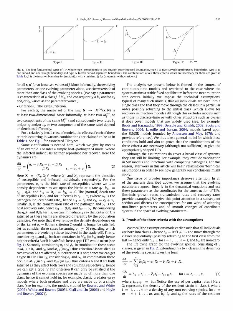
singularity, determine which evolutionary outcomes are possible.The mutational steps are sufficiently small that it is the localbehaviour of these invasion boundaries (and of the trade-off) upto quadratic approximation which we invariably describe (weavoid continually repeating this point). Subject to this, thereare four fundamental types of (singular) TIP each with theirown unique evolutionary possibilities. These are shown in Fig. 1.We call the first a type I TIP; here the invasion boundariesare both linear and superimposed. With this type of TIP onlyevolutionary attractors (for acceleratingly costly trade-offs) andevolutionary repellors (for deceleratingly costly trade-offs) arepossible. This represents the picture that emerged in early work(Levins, 1962). The second type of TIP is type II; here the invasionboundaries are again superimposed but are now curved. Againonly evolutionary attractors and repellors are possible, but nowfor weakly deceleratingly costly trade-offs attractors can replacerepellors or for weakly acceleratingly costly trade-offs repellorscan replace attractors. In type III and type IV TIPs, the invasionboundaries are no longer superimposed. In type III one boundaryis linear with the second boundary curved, whereas in type IV bothinvasion boundaries are curved. The separation of boundaries hassignificant implications for the evolutionary outcomes. For certaintrade-offs with curvature between the invasion boundaries eitherevolutionary branching points or Garden of Eden points (ESS-repellors) may be possible (which of these are possible dependsupon the relative curvatures of f1 and f2; see Table A.1).So the question arises as to what factors determine the shape

of the invasion boundaries and hence the type of TIP producedand evolutionary outcomes possible. Is it possible to establishcriteria – which are necessary for various types of TIPs andthe associated evolutionary possibilities – criteria which can beapplied directly, without the need for further calculation, to thedynamical specification of a broad class of models in populationecology? This is the focus of the present paper.

2. The three criteria

We assume that time is continuous, that individuals can only bein a finite number of classes (or i-states), and that the number ofindividuals is sufficiently large that a deterministic approximation

can be used. We take the dynamics to be given by the system ofordinary differential equations

dNdt= M(p(x),N)N; (1)

the components Ni of the m-dimensional column vector N are thedensities of individuals in the various classes i, thematrix elementsMij are the rates of increase of Ni per capita of class j, p is a vectorof parameters and x = (x1, x2) is a trait vector which changes asthe species evolves. Later we shall use the notation

Mi· =(Mi1 · · ·Mim

),

M·j =(M1j · · ·Mmj

),

to denote the ith row and jth column, respectively; we shall alsoabuse notation by writing M(x,N) rather than the full form inEq. (1).We distinguish terms contributing to the matrix elements as

follow

Mij = bij − δijeij − δij∑k

tki + tij.

The first term bij, defined as a reproduction term, corresponds to thereproduction (birth) rate in class i per capita of class j. Note that,if we take frequency dependent competition to act upon births,then this frequency dependence will appear in the correspondingreproduction term. The second term eii, defined as amortality term,corresponds to the mortality per capita of class i. The third termtij, defined as a transition term, corresponds to the transition ofindividuals from class j into class i per capita of class j. The term δijis the Kronecker delta. As indicated in Eq. (1) the matrix elementsMij and the individual terms underlying them can depend on thedensities N and the trait x.Throughout we take one evolving species, made up of n classes,

possibly in the presence of a number of non-evolving species,each of which may consist of multiple classes. The matrix M istherefore split into a number of square sub-matrices, one for eachspecies. The size of each sub-matrix is determined by the numberof classes the species is described by (e.g. a species of 3 classes willbe described by a 3× 3 sub-matrix) and where the main diagonalof each sub-matrix lies on the main diagonal of the matrix M. Allremaining entries of M, outside these sub-matrices, are zero. Forthe purposes of this study, we define the matrixM(n) as the n × nsub-matrix describing the evolving species (made up of n classes).Hoyle et al. (2008) hypothesised three criteria and claimed that

their occurrence in various combinations leads to a classificationof possible TIPs. These criteria were suggested on the basis of thestudy of a very limited number of specific models. Here we provetheir appropriateness for a relatively broad classes of ecologicaldynamics. (We impose some restrictions at first — but then liftmany of them.)The three criteria, which are based upon the dynamics

describing the behaviour of the model, are:• Criterion A: The Appearing CriterionAt least two of the row rate vectors Mi· are (non-constant)

functions of the trait vector x; that isMi·(x,N) 6= Mi·(x′,N)for all x, x′ for at least two values of i. (Consequently, a tijand/or bij and/or eij must vary for at least two values of i, as xvaries.) More informally, the evolving parameters, or one repeatedevolving parameter, appear in the population dynamics of differentclasses/species.• Criterion B: The Characteristic CriterionAt least two of the column rate vectorsM(n)

·j are (non-constant)functions of the trait vector x; that isM(n)·j (x,N) 6= M(n)

·j (x′,N)

A. Hoyle, R.G. Bowers / Theoretical Population Biology 74 (2008) 311–323 313

Fig. 1. The four fundamental types of TIP, where type I corresponds to two straight superimposed boundaries, type II to two curved superimposed boundaries, type III toone curved and one straight boundary and type IV to two curved separated boundaries. The combinations of our three criteria which are necessary for these are given inTable 1. (f1 is the invasion boundary for (mutant) ywith x resident; f2 for (mutant) xwith y resident.)

for all x, x′ for at least two values of j. More informally, the evolvingparameters, or one evolving parameter alone, are characteristic ofmore than one class of the evolving species. (We say a parameteris characteristic of a class j if Mij, and consequently a bij and/or eijand/or tij, varies as the parameter varies.)• Criterion C: The Rates Criterion.For each x, the image set of the map N → M(n)(x,N) is

at least two-dimensional. More informally, at least two M(n)ij , or

two components of the sameM(n)ij (and consequently two rates bij

and/or eij and/or tij, or two components of the same rate) dependon densities differently.For a relatively broad class ofmodels, the effects of each of these

criteria occurring in various combinations are claimed to be as inTable 1. See Fig. 1 for associated TIP types.Some clarification is needed here, which we give by means

of an example. Consider a simple host–pathogen SI model wherethe infected individuals neither reproduce nor recover. Here thedynamics are

dXdt=

(ax − qxX1 − cx − βxX1 γx

βxX1 cx + αx + γx

)X. (2)

Here X = (X1, X2)T where X1 and X2 represent the densitiesof susceptible and infected individuals, respectively. For theparameters, ax is the birth rate of susceptibles where we takedensity dependence to act upon the births at a rate qx; b11 =ax − qxX1 and b12 = b21 = b22 = 0. The (natural) death rateof susceptibles is cx and for infecteds is cx + αx (where αx is thepathogen induced death rate), hence e11 = cx and e22 = cx + αx.Finally, βx is the transmission rate of the pathogen and γx is thehost recovery rate, hence t21 = βxX2 and t12 = γx. By consideringthe qxX1 and βxX2 terms, we can immediately say that criterion C issatisfied as these terms are affected differently by the populationdensities. We note that if we remove the density dependence onbirths, i.e. set qx = 0, then criterion C would no longer be satisfied.Let us consider three cases (assuming qx 6= 0) regarding whichparameters are evolving (those involved in the trade-off). Firstly,considering ax and qx, both are contained inM11 (in b11) only, henceneither criteria A or B is satisfied; here a type I TIPwould occur (seeFig. 1). Secondly, considering ax and βx, in combination these occurinM11 (in b11 and t21) andM21 (in t21), thus criterionA is satisfied, astwo rows ofM are affected, but criterion B is not; hence we can geta type III TIP. Finally, considering ax and αx, in combination theseoccur inM11 (in b11) andM22 (in e22), thus criteria A and B are bothsatisfied as they affect both rows and columns, respectively; hencewe can get a type IV TIP. Criterion B can only be satisfied if thedynamics of the evolving species are made up of more than oneclass; hence it cannot hold in, for example, classic predator–preymodels where both predator and prey are made up of a singleclass (see for example, the models studied by Bowers and White(2002), White and Bowers (2005), Kisdi and Liu (2006) and Hoyleand Bowers (2007)).

The analysis we present below is framed in the context ofcontinuous time models and restricted to the case where thesystem attains a stable fixed equilibrium before the next mutationstep occurs. Initially, we impose the ‘technical’ assumptions,typical of many such models, that all individuals are born into asingle class and that they move through the classes in a particularorder possibly returning to the initial class (which allows forrecovery in infection models). Although this excludes models suchas those in discrete-time or with other attractors such as cycles,it does cover models that are widely used (see, for example,Boots and Haraguchi, 1999; Dercole and Rinaldi, 2002; Boots andBowers, 2004; Loeuille and Loreau, 2004; models based uponthe SIS/SIR models founded by Anderson and May, 1979; andprevious references).We thus take a generalmodel forwhich theseconditions hold and aim to prove that the combinations of thethree criteria are necessary (although not sufficient) to give theappropriately shaped TIPs.Although the assumptions do cover a broad class of systems,

they can still be limiting. For example, they exclude vaccinationin SIR models and infections with competing pathogens. For thisreason, later work in this article will begin relaxing our ‘technical’assumptions in order to see how generally our conclusions mightapply.One issue of broader importance deserves attention. In all

of the analysis described above, we assume that the evolvingparameters appear linearly in the dynamical equations and usethese parameters as the coordinates for the construction of TIPs.(Intrinsic growth rates, transmission rates and recovery ratesprovide examples.) We give this point attention in a subsequentsection and discuss the consequences for our work of adoptingnon-linear parameters and of smooth changes of coordinatesystem in the space of evolving parameters.

3. Proofs of the three criteria with the assumptions

We recall the assumptionsmade earlier such that all individualsare born into class 1 – hence bij = 0 if i 6= 1 – andmove through theclasses sequentially (possibly returning to the first class from thelast) — hence only t{i+1}i, for i = 1, . . . , n−1, and t1n are non-zero.The life cycle graph for the evolving species, consisting of 3

classes, is given in Fig. 2. Extending this to n classes, the dynamicsof the evolving species takes the form

dX1dt=

n∑j=1

b1jXj − e11X1 − t21X1 + t1nXn,

dXidt= ti{i−1}Xi−1 − eiiXi − t{i+1}iXi for i = 2, . . . , n, (3)

where t{n+1}n = t1n.(Notice the use of per capita rates.) HereXi represents the density of the resident strain in class i, wherei = 1, . . . , n, or a density of any non-evolving species, for i =m − n + 1, . . . ,m, and bij, eii and tij the rates of the resident

314 A. Hoyle, R.G. Bowers / Theoretical Population Biology 74 (2008) 311–323

Table 1The shape of TIP and the corresponding necessary criterion; see Fig. 1 for the geometrical forms of TIPs I–IV

Necessary criteria for each TIP type f1 boundary (x resident, y rare) f2 boundary (y resident, x rare) Separation of boundaries TIP typeA B C

– – – Straight Straight No I3 3 – Curved Curved No II3 – 3 Straight Curved Yes III3 3 3 Curved Curved Yes IV

The criteria A, B and C are the appearing criterion, characteristic criterion and the density dependent rates criterion, respectively.

Fig. 2. Life cycle for our system made up of 3 classes, subject to the assumptionsthat all individuals are born into class 1 (where births are indicated by thick lines)at a rate b1i , individuals move through the classes sequentially, possibly returningto class 1 from the last class, at rates t{i+1}i . In addition mortality rates for each classare given by eii .

strain where bij = Bij(x, X1(x), . . . , Xm(x)) and similarly for theother rates. We take only one species to be evolving, possibly inthe presence of a number of non-evolving species. However, forour present purposes we do not need to explicitly consider theequations describing the dynamics of any non-evolving species. Inthe calculation of the mutant fitness any interactions they havewith the evolving species will be contained in the bij, eii and tijterms.If we introduce a mutation of resident strain x, denoted y, into

this environment, and take it to be initially rare (at low density),then the dynamics can be written as

dY1dt=

n∑j=1

b1jYj − e11Y1 − t21Y1 + t1nYn,

dYidt= ti{i−1}Yi−1 − eiiYi − t{i+1}iYi for i = 2, . . . , n. (4)

Here Yi denotes the density of the mutant invaders in class i.Since the mutant is rare we can assume the appropriate limitsexist and ignore its densities in bij, eii and tij; we thus have bij =Bij(y, X1(x), . . . , Xm(x)) and bij

∣∣y=x = bij etc. and similarly for

derivatives.The fitness is defined as being the per capita growth rate of a

rare mutant invader and is commonly denoted as sx(y), where xdenotes the established resident strain and y the mutant invader(Metz et al., 1992). For this model the fitness, in terms of bij, eii andtij is given by

sx(y) ∝n∑i=1

[(b1i − eii)

(i−1∏j=0

t{j+1}j

)(n+1∏j=i+1

(t{j−1}j + ejj

))]. (5)

(See Appendix B.1 for the derivation of Eq. (5).)Each of the three criteria is claimed to have a specific effect

on the shape of the invasion boundaries in a TIP with resultantevolutionary repercussions. Satisfying criterion A (appearingcriterion) is necessary for the invasion boundaries to curve and/orseparate (details depend on the other criteria), satisfying criterionB (characteristic criterion) is necessary for the invasion boundaryf1, stemming from sx(y), to curve and satisfying criterion C (density

dependent rates criterion) is necessary for the invasion boundariesto separate. However, whether an effect is possible or not candependon the status of the other criteria (see Table 1). For example,to allow the possibility that invasion boundaries separate, andhence allow branching points and Garden of Eden points (ESS-repellors), it is actually necessary for both criteria A and C to besatisfied; A or C alone will not be enough.We prove below that the criteria are necessary for the said

effects by showing, for each criterion in turn, that, without it beingsatisfied, the corresponding effect on the invasion boundariescannot occur. (In each case the status of the other two criteria isirrelevant.)

3.1. Criterion A: The appearing criterion

This criterion relates to where, in the matrix M, the evolvingparameters appear, and hence for which classes/species theseparameters have a direct effect on the rate of change. Forthis criterion not to be satisfied requires that all the evolvingparameters must be contained in a single row of M; all the otherrows ofMmust not be directly affected by changes in the evolvingparameters. An equivalent explanation is that all the evolvingparameters must be contained in a single equation describing thedynamics; all other equations must not be directly affected bychanges in the evolving parameters.For the case when the evolving species is described by a single

equation (class) (i.e. n = 1) – in a Lotka–Volterra set-up, whereall evolving parameters only appear in a single class – it has beenshown that not only are branching points and Garden of Edenpoints not possible (White and Bowers, 2005) but the curvaturesof the invasion boundaries at the evolutionary singularity areequal (Bowers et al., 2005). For example, for prey evolution in apredator–prey system (where the prey dynamics consist of only asingle class), for the criterion to hold, the evolving parametersmustappear in (i.e. directly affect) both thedynamics describing thepreyand the dynamics describing the predator. This can (usually) onlyoccur when the evolving parameters affect the rate of predationand appear in both the dynamics of the prey and the dynamicsof the predator. Hence, although the predator is not evolving, itsability to predate as described by its dynamics is directly affecteddue to the evolution of the prey.We now assume that the criterion does not hold, hence only a

type I TIP should occur, and deduce the consequences.First we write the fitness as sx(y) = s(y, Xi(x)) (fitness

is determined by the mutant strain y and the densities of theestablished resident and any non-evolving species). We note herethat although the mutant strain is described by its two (evolving)traits, y1 and y2, these are linked by a trade-off, y2 = f (y1) say,and hence it is possible to reduce this to a single trait, y1 say (forthe working in this paper we do not require the trade-off to beshown explicitly). For convenience we abuse notation and dropthe subscripts and write y rather than y1 (and x rather than x1).Differentiating this both with respect to the established residentand with respect to the mutant invader, and evaluating at the

A. Hoyle, R.G. Bowers / Theoretical Population Biology 74 (2008) 311–323 315

evolutionary singularity (Metz et al., 1996a; Geritz et al., 1998),gives

∂2sx(y)∂x∂y

∣∣∣∣x∗=

m∑i=1

∂2s∂Xi∂y

∣∣∣∣x∗

dXidx

∣∣∣∣x∗, (6)

where |x∗ ⇔|y=x=x∗ . Bowers et al. (2005) show that if the mixedderivative of the fitness is zero at the evolutionary singularitythen the two invasion boundaries will have equal curvatures at x∗and hence will be superimposed (if approximated up to quadraticterms). We aim to show this is the case here by proving that thedXi/dx|x∗ are all zero.We begin with the observation that when the dynamics

describing the evolving species aremade up ofmore than one class(i.e. n > 1), it follows from our assumption that the criterion doesnot hold that, the evolving parameters cannot affect the transitionterms, tij = t{j+1}j, as these appear in two different rows ofM andhence in the dynamics describing both class j and class j+1 (or classn and class 1 for t1n); hence only the bij and eii terms can dependon the evolving parameters.Due to howwe have set up the dynamics of our model wemust

now consider two distinct cases (the evolving parameters mustappear somewhere in the dynamics of the evolving species):

3.1.1. The evolving parameters only appear in the dynamics describ-ing class 1In the present case, the evolving parameters can only appear in

the reproduction terms, bij = b1j, or the mortality term related toclass 1, e11; hence these are the only terms varying as the speciesevolves and hence the only functions of x or y.Focusing on the resident dynamics describing class 1, in

Eq. (3), and differentiating with respect to x, taking into accountthe dependencies Xi(x) and bij = Bij(x, X1(x), . . . , Xm(x)), gives

m∑j=1

∂

∂Xj

(n∑i=1

b1iXi − e11X1 − t21X1 + t1nXn

)dXjdx

+

n∑i=1

∂ b1i∂xXi −

∂ e11∂xX1 = 0. (7)

Our aim is to evaluate this at the evolutionary singularity. Thisrequires the fitness gradient.Differentiating the fitness in Eq. (5)with respect to y, evaluating

at the evolutionary singularity x∗ (Metz et al., 1996a; Geritz et al.,1998), gives

∂sx(y)∂y

∣∣∣∣x∗∝

n∑i=1

∂b1i∂y

∣∣∣∣x∗

(i−1∏j=0

t{j+1}j

)(n+1∏j=i+1

(t{j+1}j + ejj

))

−∂e11∂y

∣∣∣∣x∗(t10)

(n+1∏j=2

(t{j+1}j + ejj

)). (8)

Returning to the resident dynamics, in Eq. (3), the dynamicsdescribing classes 2 to n yield the set of equations

Xi =ti{i−1}(

t{i+1}i + eii)Xi−1 for i = 2, . . . , n. (9)

Solving these gives

Xi =

i−1∏j=1t{j+1}j

i∏j=2

(t{j+1}j + ejj

)X1, i = 2, . . . , n. (10)

Using this, we can re-write the derivative of sx(y), in Eq. (8), as

∂sx(y)∂y

∣∣∣∣x∗∝

(n∑i=1

∂b1i∂y

∣∣∣∣x∗

X∗iX∗1−∂e11∂y

∣∣∣∣x∗

)n∏j=2

(t{j+1}j + ejj

). (11)

As this is zero at the evolutionary singularity, x∗, and since t{i+1}i+eii > 0 for all i (see the discussion near Eq. (B.5)), we find thatn∑i=1

X∗i∂b1i∂y

∣∣∣∣∣x∗

= X∗1∂e11∂y

∣∣∣∣x∗. (12)

Eq. (12) allows us to simplify Eq. (7) at the singularity to give

A11dX1dx

∣∣∣∣x∗+ A12

dX2dx

∣∣∣∣x∗+ · · · + A1m

dXmdx

∣∣∣∣x∗= 0, (13)

where Aij are functions of bij, eii and tij, and their derivatives withrespect to the densities Xj, evaluated at the singularity.If we had written Eq. (1) in the appropriate form

dXidt= Fi(x, Xj(x)) for i = 1, . . . ,m, (14)

then we should have found Aij = ∂Fi/∂Xj∣∣x∗ . Similarly to Eq. (13),

since the Fi have no explicit x dependence for i > 2, we have∑j

AijdXjdx= 0 for i > 2. (15)

Thus, Eqs. (13) and (15) yield

A(dXjdx

∣∣∣∣x∗

)T= 0, (16)

where A is the Jacobian of the Fi with respect to the Xj at x∗. Sincewe assume x∗ is point stable in the population dynamics, A is non-singular and so

dXidx

∣∣∣∣x∗= 0 for i = 1, . . . ,m. (17)

Hence, returning to Eq. (6),we see that themixedderivative of sx(y)is zero at the singularity and therefore the invasion boundariesmust be superimposed. We briefly note that the result in Eq. (17)shows that at the evolutionary singularity, the population densityof all classes attains an extremum. This suggests the possibility ofoptimisation in this model, which again excludes the possibility ofco-existence of strains not only locally (which leads to branchingpoints not being possible) but also globally.The linearity of the invasion boundaries comes about by the

fact that the fitness, in Eq. (5), is linear in terms of b1i and e11(the terms containing the evolving parameters). Combining thiswith an assumption we make concerning the evolving parametersappearing linearly in the dynamics, and hence in b1i and e11, thenthe invasion boundary stemming from sx(y)will be linear in termsof the evolving parameters. Further, as the invasion boundaries aresuperimposed, the second invasion boundarymust also be straightgiving a type I TIP.

3.1.2. The evolving parameters only appear in the dynamics describ-ing class k, where k 6= 1In the case where the evolving parameters only appear in the

dynamics describing a single class which is not class 1 (i.e. a classin which there are no individuals entering through birth), they canonly exist in the mortality term, ekk (where k 6= 1) — this appearsin one class only. Following the proof through as in the case above(for k = 1), see Appendix B.2 for details, again yields the result thatthe two invasion boundaries are superimposed and linear. Thus,we have established the results in the first row of Table 1, suchthat not satisfying criterion A leads to linear and superimposedinvasion boundaries with the evolutionary consequences — thatacceleratingly costly trade-offs produce evolutionary attractorsand deceleratingly costly trade-offs lead to repellors.

316 A. Hoyle, R.G. Bowers / Theoretical Population Biology 74 (2008) 311–323

3.2. Criterion B: The characteristic criterion

This criterion again relates to the evolving parameters but nowis concerned with whether they are characteristics of more thanone class and hence appear in more than one column of M(n). Ifthis criterion is satisfied, then – provided criterion A (appearing) istoo – it is possible for the invasion boundary f1 – stemming fromsx(y) = 0 – to curve and give a type II or a type IV TIP (see Fig. 1).In contrast, if this criterion is not satisfied then it is only possibleto get a type I or a type III TIP (see Fig. 1). We again assume that thecriterion does not hold and deduce the consequences.Given that the evolving parameters are characteristics of the

same class, and hence only appear in a single column of M, thenthe rates, bij, eij and tij, affected by these parameters will all havethe same j. Looking back to the form of the fitness in Eq. (5), we seethat it is linear in terms of bij, eij and tij for a given j. In addition,taking into account our assumption earlier regarding the linearityof (the evolving) parameters, it follows that these appear linearlyin the fitness. Hence, the invasion boundary stemming from sx(y)(the f1 boundary)will be linear in terms of the evolving parameters.Satisfying criterion B is necessary in order for the f1 invasion

boundary to curve; however satisfying it is not sufficient to ensurethe boundary curves. For example, if the evolving parameters affectb12 and e11, and hence are characteristics of classes 1 and 2, theserates will still appear linearly in the fitness, in Eq. (5), and hencethe invasion boundary f1 will be straight.

3.3. Criterion C: Density dependent rates criterion

The third criterion is concerned with how all the entries M(n)ij ,

andhence bij, eii and tij, dependupon thepopulationdensities of theresident strain (and any non-evolving species). For criterion C to besatisfied requires there to be at least two density dependent ratesin the dynamics. These two (or more) rates can occur in the samebij, eii or tij term; there is no requirement for two different termsto be density dependent. In addition these (at least) two densitydependent rates must not depend upon the same densities in thesame manner.If the criterion is satisfied, then – provided criterion A

(appearing) is too – the invasion boundaries can separate,producing either a type III or type IV TIP (see Fig. 1), dependingupon whether the remaining criterion (B) is satisfied. If criterionC is not satisfied, then the boundaries cannot separate. We againuse the result (Bowers et al., 2005) that the boundaries havingequal curvature at the tip of the singular TIP (i.e. being locallysuperimposed) is equivalent to the mixed derivative of the fitnessbeing zero at the evolutionary singularity.The resultant effect on the fitness of not satisfying criterion

C is that it is only a function of the evolving parameters,which are dependent on y, and of one function X(x) (a singleXi or some combination of these densities), and hence willbe of the form sx(y) = s(y, X(x)). Thus, ∂sx(y)/∂x =

(∂s/∂X) (dX/dx) and since this derivative is zero at the singularity(Metz et al., 1996a; Geritz et al., 1998) dX/dx|x∗ = 0. Since∂2sx(y)/∂y∂x =

(∂2s/∂y∂X

)(dX/dx), this mixed derivative is zero

at the singularity.The idea that if the fitness is only a function of a single density,

and the traits of the mutant strain, then branching points andGarden of Eden points (ESS-repellors) are impossible, is not arecent one (for example, seeMetz et al. (1996b), Heino et al. (1998),Kisdi (1998) and Rueffler et al. (2006)). A fitness of this formhas been called one-dimensional feedback environment, frequencyindependent and ‘trivial’ frequency dependence (see previousreferences). The benefit of taking this idea one step back (from thefitness to the dynamics) is that whether separation of boundariesis possible or not can be determinedwithout carrying out the oftencomplex calculations in order to find the fitness function.

Fig. 3. Life cycle for a system made up of 2 classes (where births are indicated bythick lines at a rate bij — rate at which individuals in class j give birth to individualsin class i). The assumption stating that all individuals are born into class 1 has nowbeen relaxed. In additionmortality rates for each class are given by eii and transitionrate by tij .

4. Relaxing the technical assumptions

In the above analysis a number of ‘technical’ assumptions weremade, in particular: that all individuals enter into class 1 and thenmay move through the classes sequentially, eventually possiblyreturning to class 1 from the last class. However, inmany ecologicalsystems these are not the case. By relaxing the assumptions in turn,we will test whether each of our three criteria still hold.

4.1. Individuals born into different classes

We begin by holding to the assumption regarding individualsmoving through the classes in order. However, we relax theassumption concerning into which class individuals are born.Previously we had all new individuals entering into class 1.However, if we consider SIR systems, vertical transmission ornatural immunity can lead to offspring directly entering theinfected or recovered class, respectively. Taking this into account,the dynamics (of our evolving species) now take the form

dXidt=

n∑j=1

bijXj − eiiXi − t{i+1}iXi + ti{i−1}Xi−1,

for i = 1, . . . , n (18)

where we replace +t10X0, for j = 1, and −t{n+1}nXn, for j = n,with ±t1nXn, respectively, so that ‘cycling’ is explicitly included.For simplifying purposes we take n = 2, i.e. the evolving speciesonly consists of two classes. Fig. 3 shows the life cycle graph forthis model. If we introduce a mutation in the evolving species, thedynamics of the rare invader will take the form

dY1dt= b11Y1 + b12Y2 − e11Y1 − t21Y1 + t12Y2,

dY2dt= b21Y1 + b22Y2 − e22Y2 − t12Y2 + t21Y1. (19)

We can show that although the current assumption has beenrelaxed, the three criteria still hold, in that satisfying them allowsthe relevant TIP type, and resultant evolutionary outcomes, to bepossible (see Appendix C.1 for details). Although this is limited ton = 2, we expect that the results will apply more generally.

4.2. Individuals do not move through classes in order

Previously, we made an assumption that individuals movethrough the classes sequentially, perhaps returning to the firstclass from the last. However, in a number of ecological systems thisis not always the case. For example, in an SIR model, individualscan be born into the susceptible class and from there they can be

A. Hoyle, R.G. Bowers / Theoretical Population Biology 74 (2008) 311–323 317

Fig. 4. Life cycle for a systemmadeup of 3 classes, subject to the assumption that allindividuals are born into class 1 (where births are indicated by thick lines) at a ratebij . The assumption stating that individuals move through the classes sequentiallyhas now been relaxed and they move from class j to class i at a rate tij . In additionmortality rates for each class are given by eii .

infected, moving into the infected class, or they can be vaccinated,moving straight to the immune (removed) class avoiding theinfected class completely. For this reason, we now take a modelwhere we again assume that all individuals are born into class 1;however, we allow movement between any class (i.e. they beginin class 1 and from there they can move to any of the other n − 1classes, fromwhich they can againmove to any of the n−1 classes).Here the dynamics (of our evolving species) take the form

dX1dt=

n∑j=1

b1jXj − e11X1 +n∑j=1

(t1jXj − tj1X1

),

dXidt= −eiiXi +

n∑j=1

(tijXj − tjiXi

)for i = 2, . . . , n. (20)

For simplicity, we take a system where the evolving speciesconsists of 3 classes as this is the smallest number which createsdifferences in the dynamics from the previous models. The lifecycle graph is shown in Fig. 4. In this model, a (rare) invader strainwill have dynamics

dY1dt=

3∑i=1

b1iYi − e11Y1 +3∑i=1

(t1iYi − ti1Y1) ,

dY2dt= −e22Y2 +

3∑i=1

(t2iYi − ti2Y2) ,

dY3dt= −e33Y3 +

3∑i=1

(t3iYi − ti3Y3) .

(21)

We can again show that although the assumption has been relaxedthe three criteria still hold, giving the possible TIPs stated inTable 1 and respective evolutionary outcomes (see Appendix C.2for details).

5. Evolving parameters: Non-linearities and coordinate change

In many systems (for example, Bowers et al. (2003) andWhite and Bowers (2005)) evolving parameters which are used ascoordinates in presenting our TIPs may be identified on biologicalgrounds – per capita low density birth rates or recovery rates frominfection – and then observed to appear linearly in the dynamics.Despite this there are two interrelated reasons for investigating theeffects on our criteria of parameters which enter M non-linearly.First, in more complex settings, parameters of direct biologicalimportance may enter non-linearly — an example of this appearsin studies of the evolution of predator handling time using aHolling Type II functional response (Holling, 1959; Kisdi and Liu,2006; Hoyle and Bowers, 2007; Geritz et al., 2007). Second, it

may be inappropriate to afford certain parameters – in particularthose entering linearly – a privileged position on the basis of anotion of ’direct biological importance’. For example, why shoulda recovery rate be stressed rather than the corresponding durationof infection? This perspective stresses those aspects of our analysiswhich are invariant under appropriate smooth coordinate changein the space of evolving parameters. Invariably, coordinate changewill produce ’new parameters’ which enter the dynamics non-linearly; the issues are essentially the same.In the models we have studied so far – with the evolving

parameters (adopted as coordinates) appearing linearly – notsatisfying criterion A results in the invasion boundaries being bothlinear and superimposed. If we remove the assumption that theevolving parameters appear linearly, we can still use the methodof Section 3.1 to show that, when criterion A is not satisfied, theinvasion boundaries are superimposed (the argument makes noassumption about parameter linearity). However, the argumentshowing that when criterion A is not satisfied, the invasionboundaries are linear does depend on the parameter linearity; thisproperty is not generic under parameter choice. Generically, notsatisfying criterion A gives a type II TIP with type I as a degeneratecase.In the models we have studied so far – with the evolving

parameters appearing linearly – not satisfying criterion B results inthe invasion boundary f1 being linear. If we remove the assumptionthat the evolving parameters appear linearly, this conclusion nolonger applies. (The fitness is no longer linear in the evolvingparameters.) Hence, generically, this criterion has no power.In the same context, criterion C still applies. The argument in

Section 3.3 is unaffected by parameter non-linearity. Thus, gener-ically not satisfying criterion C implies superimposed boundarieswhich again means a type II TIP with type I as a degenerate case.The final conclusion that can be drawn is that both criteria A and

C are necessary for separated boundaries which result in a type IVTIP, the degenerate case now being type III.However, despite the criteria only being partially valid in the

above cases,we emphasise the significance of the three criteria andthe resultant classification of the four TIP types in the importantcases where the parameters are linear.

6. Discussion

Trade-off and invasion plots (TIPs) (Bowers et al., 2005) weredeveloped as a graphical alternative, which keeps the trade-offexplicit, to the traditional approach to adaptive dynamics (Metzet al., 1996a; Geritz et al., 1998). The key determining factor ofwhich evolutionary outcome occurs is the respective curvaturesof the trade-off and the invasion boundaries. Hoyle et al. (2008)introduced four fundamental types of TIP (Fig. 1), each withimmediate consequences for the possible evolutionary behaviour.In addition, these authors introduced three criteria (based onvarious aspects of continuous time models) and claimed, on thebasis of a few model calculations, that their occurrence in variouscombinations leads to a classification of possible TIPs. Thesethree criteria were the appearing criterion (A), the characteristiccriterion (B) and the density dependent rates criterion (C). Thecombinations of these criteria and the respective TIPs producedare shown in Table 1 and Fig. 1. We have presented proofs of theseclaims for a relatively general continuous time set-up. Our analysisinitially depended on various assumptions: (i) that all individualsenter class 1 and (ii) then move through the classes sequentially,possibly returning to class 1 from the final class, and (iii) that theevolving parameters appear linearly in the dynamics.A key feature shown however is that although the criteria

are necessary to gain each type of TIP, they are not sufficientto guarantee that type. For example, suppose we return to the

318 A. Hoyle, R.G. Bowers / Theoretical Population Biology 74 (2008) 311–323

Fig. 5. An example of each of the four types of TIP with the evolutionary outcomes for each region given, with the outcome occurring being determined by which region thetrade-off, f , enters. In each TIP here the trade-off is a weakly acceleratingly costly trade-off and the evolutionary singularity, x∗ , is an attractor for the type I, type II and typeIII TIPs, and a branching point for the type IV TIP. (f1 is the invasion boundary for (mutant) ywith x resident; f2 for (mutant) xwith y resident; the ‘dashed’ curve representsthe mean curvature of f1 and f2 .)

dynamics in Eq. (3) and take a situation where the evolvingparameters are contained in the terms b1i and e{i−1}{i−1} (a trade-offbetween the birth rate from individuals in class i and the death rateof individuals in class i− 1). Here, the evolving parameters appearin (directly affect) the dynamics describing more than one class(satisfying criterion A) and are characteristics of different classes(satisfying criterion B), therefore we might expect to gain a type II(i.e. two curved, superimposed boundaries) or type IV TIP (i.e. twocurved, separated boundaries). However, because b1i and e{i−1}{i−1}appear in the fitness, sx(y) in Eq. (5), linearly (i.e. bi does notmultiply e{i−1}{i−1}), the invasion boundary stemming from sx(y)will be linear in terms of evolving parameters (as these appearlinearly in b1i and e{i−1}{i−1}). Therefore, the TIPwill either have twostraight, superimposed invasion boundaries (type I) or one straightand one curved boundary (type III). Hence, being characteristic ofdifferent classes is necessary for the boundary stemming from sx(y)to curve, but it is not sufficient for this to be the case.In order to expand the spectrum of models where our criteria

(might) hold, for example to SIR systemswith vertical transmissionor vaccination, we relaxed each of the main three assumptions inturn. We showed that if we relaxed the assumptions regardinginto which classes new individuals enter and the order in whichindividuals move through the classes, then the three criteria stillapplied for cases when the evolving species were made up of 2and 3 classes, respectively. We expect that the criteria will holdfor cases when the evolving species is made up of any number ofclasses.When we relaxed the final assumption, that the evolving

parameters enter the dynamics linearly, to allow for examplefor handling times in a Holling Type II functional response inpredator–prey systems and smooth coordinate changes, we foundthat although criterion C still holds, criteria A and B fail. Concerningcriterion A however, if the evolving parameters only appear in asingle class, then the part of the criterion stating that the invasionboundaries are superimposed holds; however the part statingthat the boundaries are straight fails. Therefore, where previouslynot satisfying criterion A gave a type I TIP only, if the evolvingparameters appear non-linearly then this now gives either a type Ior type II TIP. The only way to get a type III or type IV TIP is if bothcriteria A and C are satisfied; if either (or neither) are satisfied, thenonly type I or type II TIPs are possible. Here criterion B does not playa part in which type of TIP is produced.Prior to this work the link between TIPs and evolutionary

behaviour had already been obtained by adding trade-off curves toa TIP (see Fig. 5 for an example) as discussed fully in Bowers et al.(2005).Wenow link the occurrence or otherwise of criteria A, B andC directly to evolutionary behaviour in more detail using the TIP asa link. This works for a relatively broad class of ecological systemsdescribed near Eq. (3), made broader by our later extensions.Thus, for systems in which the evolving parameters directly affectonly one class/species (not A — e.g. ax and qx in Eq. (2)), or

those in which the evolving parameters do affect more than oneclass/species, the evolving parameters are characteristics of onlyone class, and the rates are dependent on only one density orcombination of densities (which are therefore A, not B, not C —e.g. ax and βx in Eq. (2) with qx = 0), we have a type I TIP and henceacceleratingly costly trade-offs lead to evolutionary attractors anddeceleratingly costly trade-offs lead to evolutionary repellors (asseen in Fig. 5- Type I). Systems inwhich both the parameter criteriaare satisfied but the rates remain dependent on only one densityor combination of densities (which are therefore A, B, not C —e.g. ax and αx in Eq. (2) with qx = 0) may be type II when,if the superimposed invasion boundaries curve in the manner inFig. 5, strongly deceleratingly costly trade-offs lead to repellors,and weakly deceleratingly costly and acceleratingly costly trade-offs lead to attractors (and correspondingly). Systems in which thefirst (appearing) parameter criterion and the rates criterion aresatisfied but the evolving parameters remain characteristic of onlyone class (A, not B, C — e.g. ax and βx Eq. (2)) may be Type IIIwhen, if the f2 boundary curves as in Fig. 5, strongly deceleratingcostly trade-offs lead to repellors, acceleratingly costly trade-offslead to attractors but weakly deceleratingly costly trade-offs nowlead to branching points. Finally, systems in which all the criteriaare satisfied (A, B, C — e.g. ax and αx in Eq. (2)) may be type IVwhen, if the configuration is as in Fig. 5, in addition to the typeIII results, weakly acceleratingly costly trade-offs may also yieldbranching points. Although branching points have been shown forcertain regions between the two invasion boundaries, in Fig. 5,Garden of Eden points (ESS-repellors) may occur instead. Which ofthese, branching points or Garden of Edenpoints, occur for relevantshaped trade-offs depends upon the relative curvatures of theinvasion boundaries at the evolutionary singularity (i.e. whetherthe curvature of f1 is greater than that of f2, or vice-versa, near x∗)and the signs of the fitness functions on either side of the invasionboundaries (e.g. whether sx∗(y) > 0 above or below the f1 invasionboundary). The possible evolutionary outcomes for the variousshapes of trade-off for each possible configuration are shown inTable A.1.Since the occurrence of branching points is linked to dimor-

phism and possibly speciation (Metz et al., 1996a; Geritz et al.,1998; Doebeli and Dieckmann, 2000), it is intriguing to observethat necessary conditions for these are that the evolving parame-ters directly affect not only one class/species (A) and that the ratesare not dependent on only one density or combination of densi-ties (C). Whether these apply or not can be obtained directly fromthe model without the need for further calculation. Given theseand weakly deceleratingly costly trade-offs (type III, A, not B, C)or appropriate trade-offs of intermediate strength (type IV, A, B, C)branching points are possible for the class of system studied here;they are not otherwise.

A. Hoyle, R.G. Bowers / Theoretical Population Biology 74 (2008) 311–323 319

Acknowledgments

We wish to thank the reviewers for very useful comments onearlier drafts of this article; we are also grateful to Dr. A.White andProf. M. Boots for many helpful conversations.

Appendix A. Trade-off and invasion plots (TIPs)

A detailed description of the use of trade-off and invasionplots (TIPs) to determine evolutionary behaviour has been givenelsewhere (Bowers et al., 2005). Here we will give a brief outlineof TIPs and present some of the results/conditions for determiningthe evolutionary behaviour of a system.Trade-off and invasion plots are a geometrical approach that

makes the role that different trade-off shapes play easy to visualise.A TIP is a plot between two (competing) strains of a species,labelled x and y say. One of these, x, is taken to be fixed whilethe second, y, is allowed to vary. The axes of a TIP are the twoevolving parameters (or traits) of the y strain, y1 and y2 (only twoparameters are taken to vary). The co-ordinates x1 and x2 of thefixed strain x define the corner or tip of a TIP. Examples of TIPs(including the evolutionary outcomes for each region) can be seenin Fig. 5.Two of the three curves on a TIP are the invasion boundaries,

denoted as f1 and f2. These curves denote where sx(y) = 0 andsy(x) = 0, respectively, and hence into regions where the varyingstrain y can and cannot invade the fixed strain x (either side of f1 —where sx(y) > 0 and sx(y) < 0, respectively) and where the fixedstrain x can and cannot invade the varying strain y (either side off2 — where sy(x) > 0 and sy(x) < 0, respectively). Both of theseinvasion boundaries pass through the tip of a TIP (where y = x)at which they are tangential. The third curve on a TIP is the trade-off curve, denoted as f ; this links the two evolving parameters ofeach strain. This curve also passes through the tip of a TIP, butnot usually tangentially to the invasion boundaries. Importantly,as all the feasible pairs of traits (and hence strains) lie on his curve,the side of the invasion boundaries in which the trade-off entersa TIP determines whether each strain can invade the other (wheninitially rare).For certain TIPs corresponding to particular values x∗ of x, the

trade-off curve can become tangential to the invasion boundariesat the tip of a TIP (i.e. where y = x = x∗); these valuesof x are evolutionary singularities, with the corresponding TIPsbeing singular TIPs (Fig. 5). It is from these singular TIPs that theevolutionary behaviour of a system is determined. The invasionboundaries (and their mean curvature) separate the singularTIP into regions, each with their own respective evolutionarybehaviour. (If a singular point does not exist, then invadabilitywill prefer either always higher or always lower values of x. Ifmore than one singular point exists then a separate TIP must beconsidered at each singular point.) Due to the coincidence andmutual tangential property of the three curves at the tip of asingular TIP, the region in which the trade-off curve enters (andhence the evolutionary behaviour) is determined solely by thecurvatures of the three curves; or more specifically, the curvatureof the trade-off in relation to those of the invasion boundaries atthe evolutionary singularity (as in standard theory mutations areassumed to be small). The two significant relations are betweenthe trade-off and f1 for evolutionary stability ESS and between thetrade-off and the mean curvature of both f1 and f2 for convergentstability CS. These can be written

ESS⇔ λ1f ′′(x∗) < λ1∂2f1∂y2

∣∣∣∣x∗, (A.1)

CS⇔ λ1f ′′(x∗) <λ1

2

(∂2f1∂y2

∣∣∣∣x∗+∂2f2∂y2

∣∣∣∣x∗

)(A.2)

Table A.1Shapes of trade-off (in relation to the invasion boundaries f1 and f2) required toproduction each evolutionary outcome, given a particular sign of λ1 and λ2

λ1λ2 > 0 λ1λ2 < 0

λ2f ′′ < λ2f ′′1 Attractor Repellorλ2f ′′1 < λ2f ′′ < λ2

12

(f ′′1 + f

′′

2

)Branching point Garden of Eden point

λ2f ′′ > λ212

(f ′′1 + f

′′

2

)Repellor Attractor

Here λ1 = sign (sx∗ (y)) just above the invasion boundary f1 , λ2 =

sign(∂2f2/∂y2

∣∣x∗ − ∂2f1/∂y2

∣∣x∗)and f ′′i = ∂2fi/∂y2

∣∣x∗ for n = 1, 2.

where λ1 = sign (sx∗(y)) just above the invasion boundary f1. Hereλ1 concerns how the fitness varies as we move vertically up a TIP(i.e. aswe vary the parameter on the vertical axis). Combinations ofthese properties allow the evolutionary behaviour of the system tobe determined. The possible types of singularity are evolutionaryattractors or CSS (continuously stable strategy). (ESS and CS),evolutionary branching point (CS but not an ESS), ‘Garden of Eden’point or ESS-repellor (ESS but not CS) and evolutionary repellor(neither ESS nor CS). The shapes of trade-off which lead to eachof these are given in Table A.1. These conditions for ES and CSremain invariant under smooth changes of coordinates; hence ifa particular evolutionary outcome occurs in one coordinate space,then it will occur in all. Examples of how these appear on a singularTIP are given in Fig. 5 for each of the four fundamental types of TIP.

Appendix B. Including assumptions regarding the birth andmovement of individuals

B.1. Derivation of the fitness function

The fitness is defined as being the per capita growth rate of arare mutant invader and is commonly denoted as sx(y), where xdenotes the established resident strain and y the mutant invader(Metz et al., 1992). This fitness, or a sign equivalent version ofit, can be found in a number of ways. A traditional method is touse r , the maximum eigenvalue of the invasion Jacobian (Metzet al., 1996a; Geritz et al., 1998). An alternative, which is signequivalent, is to use R0 − 1, where R0 is the maximum eigenvalueof the next generation matrix. (Diekmann and Heesterbeek (2000)describe this equivalence in an epidemiological context.) TakingG as the transition matrix whose elements are the net ratesof increase in individuals of class i per individual of class j(excluding reproduction terms) (Reade et al., 1998; Diekmann andHeesterbeek, 2000), the average times Tij, which an individual bornin class j spends in class i, are identified as the elements of −G−1.Hence, the next generation matrix is−bTG−1, where the elementsof b are the per capita reproduction rates.An assumption wemake initially is that all individuals are born

into a single class, this being class 1. In this case all but the firstrow of b are null. Therefore, the next generationmatrix has a singlenon-zero eigenvalue R0 and the fitness is

R0 − 1 =n∑i=1

b1iTi1 − 1 =n∑i=1

(b1i − eii)Ti1. (B.1)

The second equality here can be established formally as follows:The columns of G sum to the−eii (since the diagonal elements are−(eii +

∑j tij)) and hence det(G) = −

∑i eiiC1i, where the Cij are

cofactors. Thus,n∑i=1

eiiTi1 = −1|G|

n∑i=1

eiiC1i = 1, (B.2)

as required. Thus, from Eq. (B.1), in the present form we can writedown a sign equivalent fitness satisfying

320 A. Hoyle, R.G. Bowers / Theoretical Population Biology 74 (2008) 311–323

sx(y) ∝n∑i=1

ρiTi. (B.3)

Here we drop the second subscript and note that the growth rateterms, ρi, simply take the form b1i− eii, i.e. the difference betweenthe reproduction terms and mortality terms corresponding toindividuals in class i. We highlight here that these growth rates donot involve the transition terms, tij, as these are the rate at whichindividuals move from one class to the next and hence remain inthe systemwithout affecting the total population. For cases wherethe evolving species is made up of a single class (i.e. n = 1 in thedynamics above), the only class is Y1 whichwill have the dynamics(b11 − e11)Y1; hence the fitness will simply be the limit as Y1 → 0of b11 − e11, i.e. of the difference between the reproduction andmortality terms.Returning to our calculations for Ti, initially, an individual is

born into class 1 and moves through the classes sequentially.Hence, as it moves through the classes from 1 to n, the equationsgiving the time spent in each class, in terms of our mortality andtransition terms are

1 =k∑i=1

eiiTi + t{k+1}kTk for k = 1, . . . , n, (B.4)

where here we have assumed that t{n+1}n = 0 so that individualscannot return to class 1 from class n. Eq. (B.4) can be supportedphenomenologically since they equate to unity the probability ofleaving (by mortality or transition to the next class) cumulativelyto the end of each successive class. They can also be establishedformally from −GT = I in the case of sequential movementthrough the classes with no cycling.The solution of Eq. (B.4), representing the average time spent in

class i, is given by

Ti =

i−1∏j=0

(t{j+1}j

)i∏j=1

(t{j+1}j + ejj

) where t10 = 1. (B.5)

Here we assume t{i+1}i + eii > 0 for all i (i.e. that individuals canleave every class either through mortality or moving to the nextclass).Combining the times in Eq. (B.5) with the rates ρi = b1i − eii in

the form of the fitness in Eq. (B.3) gives

sx(y) ∝n∑i=1

(b1i − eii)

i−1∏j=0

(t{j+1}j

)i∏j=1

(t{j+1}j + ejj

) . (B.6)

If we omit a positive common denominator,∏n+1j=1

(t{j+1}j + ejj

)where (t{n+2}{n+1}+ e{n+1}{n+1}) = 1, then we can write the fitnessas

sx(y) ∝n∑i=1

[(b1i − eii)

(i−1∏j=0

t{j+1}j

)(n+1∏j=i+1

(t{j+1}j + ejj

))]. (B.7)

It is this form for the fitness (also shown in Eq. (5)) that we use toprove the three criteria introduced in the main text.We later relax some of the assumptions underlying Eq. (B.7).

With such generalisations in mind, it is worth observing thatEq. (B.7) already includes the case of sequentialmovement throughclasses but with tn 6= 0 so that returning to the initialclass is possible as in some infectious models with recovery.Phenomenologically this can be established by regarding Eq. (B.4)

as giving the time for the first pass T (1)i . After returning to class 1,the individuals move through the classes for a second time (andsubsequently a third and fourth time and so on) during which theaverage time spent in each class will be T (2)i (and T (3)i , T

(4)i and so

on). The total average time an individual will spend in each classwill be Ti =

∑∞

j=1 T(j)i (i.e. the sum of the times it spends in class i

during each pass through). However, this is the sum of a geometricseries and each total takes the form Ti =

∑j T(j)i = AT

(1)i , where A

is the same (positive) factor for all i. Hence the fitness, which takesthe form sx(y) ∝

∑i ρiTi can be written as sx(y) ∝ A

∑i ρiT

(1)i .

Omitting the (positive) constant A, we can take the times T (1)i asour Ti for the fitness, omittingA from further calculations. Formally,−GT = I givesn−1 equations for the ratios Ti/T1which correspondto those derived from Eq. (B.4). Although T1 is not as at Eq. (B.4), itmay be omitted from Eq. (B.3) by removing it as a positive factorleaving an expression in the above ratios.

B.2. Criterion A — The evolving parameters only appears in thedynamics describing class k, where k 6= 1

In Section 3.1.1 we showed that if the evolving parametersonly appear in the dynamics describing a single class and thatwas class 1, then the invasion boundaries would always be linearand superimposed. Here we again take the evolving parameters toappear in the dynamics describing a single class, but this time it isnot class 1.Again we aim to show that ∂Xi/∂x|x∗ = 0 for all i, however, in

this case, the evolving parameters can only exist in the mortalityterms, ei (where i 6= 1) — these appear in the dynamics describingone class only. Let us assume that this is class k, where k 6= 1, andhence only in ekk.Focusing on the resident dynamics for the class k, we find that

Eq. (7) is replaced by∑j

(∂Fk∂Xj

)dXjdx−∂ekk∂xXk = 0. (B.8)

Differentiating the fitness in Eq. (B.7)with respect to themutantinvader y and evaluating at the evolutionary singularity, gives

∂sx(y)∂y

∣∣∣∣x∗∝∂ekk∂y

∣∣∣∣x∗

[−

(k−1∏j=0

t{j+1}j

)(n+1∏j=k+1

(t{j+1}j + ejj

))

+

k−1∑i=1

(b1i − eii)

(i−1∏j=0

t{j+1}j

)(k−1∏j=i+1

(t{j+1}j + ejj

))

×

(n+1∏j=k+1

(t{j+1}j + ejj

))]∣∣∣∣∣x∗

= 0, (B.9)

since only ekk is taken to vary as y changes. Using the form for thedensities in Eq. (10) this can be re-written as

∂ekk∂y

∣∣∣∣x∗

(n+1∏j=k+1

(t{j+1}j + ejj

)∣∣x∗

)[−

(XkX1

k∏j=2

(t{j+1}j + ejj

))

+

k−1∑i=1

(b1i − eii

) XiX1

(k−1∏j=2

(t{j+1}j + ejj

))]∣∣∣∣∣x∗

= 0. (B.10)

With some simplifying, this becomes

∂ekk∂y

∣∣∣∣x∗

1X1

(k−1∏j=2

(t{j+1}j + ejj

)∣∣x∗

)(n+1∏j=k+1

(t{j+1}j + ejj

)∣∣x∗

)

×

[−Xk

(t{k+1}k + ekk

)+

k−1∑i=1

(b1i − eii

)Xi

]∣∣∣∣∣x∗

= 0. (B.11)

A. Hoyle, R.G. Bowers / Theoretical Population Biology 74 (2008) 311–323 321

Using the fact that eiiXi = ti{i−1}Xi−1− t{i+1}iXi (see Eq. (9)) and thatX1 > 0 and t{i+1}i + eii > 0 for all i, gives

∂ekk∂y

∣∣∣∣x∗

[−Xk

(t{k+1}k + ekk

)+ tk{k−1}Xk−1

− t21X1 − e11X1 +k−1∑i=1

b1iXi

]∣∣∣∣∣x∗

= 0. (B.12)

Again using the equilibrium conditions ekkXk = tk{k−1}Xk−1 −t{k+1}kXk and that derived from dX1/dt = 0, simplifies this to

∂ekk∂y

∣∣∣∣x∗

[−t1nXn −

n∑i=k

b1iXi

]∣∣∣∣∣x∗

= 0. (B.13)

Thus,

∂ekk∂y

∣∣∣∣x∗= 0, (B.14)

and Eq. (B.8) simplifies at the singularity to give

Ak1dX1dx+ · · · + Akm

dXmdx= 0. (B.15)

The remainder of the proof showing that the two invasionboundaries are superimposed and linear is identical to that for theprevious case, in Section 3.1.1.

Appendix C. Relaxing the technical assumptions

C.1. Individuals enter the system through any class

Here we calculate the fitness and determine whether the threecriteria still holdwhenwe relax the constraint limitingwhich classindividuals can be born into.Earlier we noted that the fitness can be found by a number of

methods. Elsewhere here we have used a census of the populationin the next generation following an invasion. This method isequivalent to identifying the fitness with R0 − 1 where R0 is themaximum eigenvalue of the next generation matrix (Diekmannand Heesterbeek, 2000). When we relax the assumption regardingreproduction, this is computationally difficult; hence here weprefer to use r , the maximum eigenvalue of the invasion Jacobian(Metz et al., 1996a; Geritz et al., 1998).Calculating the Jacobianmatrix for themutant dynamics above,

in Eq. (19) and evaluating each entry at the equilibrium for theestablished resident existing alone (i.e. with Y1 = Y2 = 0) gives

J =(b11 − e11 − t21 b12 + t12b21 + t21 b22 − e22 − t12

). (C.1)

The off-diagonal elements of J are positive; hence we have tworeal eigenvalues. The entries on the main diagonal are negative(due to the equilibrium conditions of

(b11 − e11 − t21

)X1 =

−(b12 + t12

)X2 etc.); hence so is the trace of this matrix and the

minimum eigenvalue. Thus, r and−det(J) are sign equivalent andwe can use the latter as a substitute fitness so

sx(y) ∝ − (b11 − e11 − t21) (b22 − e22 − t12)+ (b12 + t12) (b21 + t21) . (C.2)

Using this form we go on to examine whether the three criteriahold when the assumption as to which class newborn individualsenter is relaxed.

C.1.1. Criterion A: The appearing criterionFirst we consider criterion A (appearing) and assume this

criterion is not satisfied, hence all the evolving parameters appearin the dynamics describing a single class only, which, because ofsymmetry, we take without loss of generality to be class 1. Theevolving parameters can only appear in the terms b1i and e11. Theanalogue of Eq. (8) is

∂sx(y)∂y

∣∣∣∣x∗∝ −

(∂b11∂y

∣∣∣∣x∗−∂e11∂y

∣∣∣∣x∗

)(b22 − e22 − t12)

+∂b12∂y

∣∣∣∣x∗(b21 + t21) = 0. (C.3)

Using the equilibrium derived from the dynamics describing class2 (i.e. (b21 + t21)X1 + (b22 − e22 − t12)X2 = 0) this can be writtenas∂sx(y)∂y

∣∣∣∣x∗∝ −(t21 + b21)

×

((∂b11∂y

∣∣∣∣x∗−∂e11∂y

∣∣∣∣x∗

)X1X2+∂b12∂y

∣∣∣∣x∗

)= 0. (C.4)

As this derivative is zero at the evolutionary singularity andassuming t21+ b21 > 0 (i.e. that individuals from class 1 can moveto or create offspring into class 2), we get the equality

∂b11∂y

∣∣∣∣x∗X1 +

∂b12∂y

∣∣∣∣x∗X2 =

∂e11∂y

∣∣∣∣x∗X1. (C.5)

Returning to the equilibrium condition for class 1, from Eq. (18),we findm∑i=1

∂

∂Xi

(b11X1 + b12X2 − e11X1 − t21X1 + t12X2

) dXidx

+

(∂ b11∂x−∂ e11∂x

)X1 +

∂ b12∂xX2 = 0. (C.6)

Evaluating this as the evolutionary singularity, and using Eq. (C.5),we can write this as

A11dX1dx

∣∣∣∣x∗+ A12

dX2dx

∣∣∣∣x∗+ · · · + A1m

dXmdx

∣∣∣∣x∗= 0. (C.7)

The remainder of the argument parallels that in Section 3.1.1 —hence the criterion holds.

C.1.2. Criterion B: The characteristic criterionFocusing on those terms which are characteristic of class 1

(without loss of generality) in the fitness in Eq. (C.2) (the termswith second subscript being 1), the rates b1i, e11 and t21 againappear linearly. Therefore, the invasion boundary f1 is againstraight. Hence, this criterion holds.

C.1.3. Criterion C: Density dependent rates criterionThe argument we introduced in Section 3.3 also holds when we

allow newborn individuals to enter the system through any class,hence this criterion holds.

C.2. Individuals can move between classes in any order

Here we calculate the fitness and determine whether thethree criteria still hold when we relax the constraint stating thatindividuals move through the classes sequentially.To calculate the fitness we use the approach as earlier, in

Eq. (B.3); however relaxing the present assumption makes theaverage time a mutant individual spends in each class morecomplicated. To find the average times we must now turn to a

322 A. Hoyle, R.G. Bowers / Theoretical Population Biology 74 (2008) 311–323

more general approach involving the transition matrix G (Readeet al., 1998; Diekmann and Heesterbeek, 2000). The elements ofthis matrix, Gij, are the net rates of increase in individuals of classi per individual in class j (excluding birth terms). For the explicitmodel in Eq. (21), we have

G =

(−e11 − t21 − t31 t12 t13

t21 −e22 − t12 − t32 t23t31 t32 −e33 − t13 − t23

).

(C.8)The average times Tij which an individual born in class j spends inclass i, are identified as the elements of−G−1 and hence

− G−1 = −1|G|

×

((e22 + t21 + t23)(e33 + t31 + t32)− t23t32 · · · · · ·

t13t32 + t12(e33 + t31 + t32) · · · · · ·

t12t23 + t13(e22 + t21 + t23) · · · · · ·

), (C.9)

where |G| < 0. As all individuals enter the system into class 1, weonly require the times that appear in the first columnof thismatrix.Combining the times in Eq. (C.9) with the rates ρi = b1i− eii, givesthe fitness assx(y) ∝ (b11 − e11) ((e22 + t2)(e33 + t3)− t23t32)

+ (b12 − e22) (e33t21 + t1t3 − t13t31)+ (b13 − e33) (e22t31 + t1t2 − t12t21) , (C.10)

where t1 = t21 + t31, t2 = t12 + t32 and t3 = t13 + t23 and we havedropped the positive factor−1/|G|.

C.2.1. Appearing criterionWe aim to establish the result in Eq. (17) in this new context

and hence use Eq. (6) to show that the invasion boundaries aresuperimposed.We now assume that the evolving parameters only appear in

the dynamics describing a single class. First we assume that this isclass 1; then only rates b1i (for i = 1, 2, 3) and e11 change as theseparameters change. Hence,

∂sx(y)∂y

∣∣∣∣x∗∝

(∂b11∂y−∂e11∂y+∂b12∂yT2T1+∂b13∂yT3T1

)∣∣∣∣x∗= 0, (C.11)

where we have returned to the form Ti for the times for simplicity(as these do not contain b1i or e11). Returning to the residentdynamics in Eq. (20) at equilibrium we getX2(e22 + t2) = t21X1 + t23X3,

X3(e33 + t3) = t31X1 + t32X2. (C.12)Rearranging these, we can write the (ratios of) equilibria in termsof the average times spent in each class as

X2X1=T2T1

andX3X1=T3T1. (C.13)

Eqs. (C.11) and (C.13) give∂sx(y)∂y

∣∣∣∣x∗∝∂b11∂y

∣∣∣∣x∗−∂e11∂y

∣∣∣∣x∗+∂b12∂y

∣∣∣∣x∗

X∗2X∗1

+∂b13∂y

∣∣∣∣x∗

X∗3X∗1= 0. (C.14)

Taking the dynamics describing class 1 of the resident strain (setat equilibrium) differentiated through with respect to the residentstrain and evaluated at the evolutionary singularity, givesm∑j=1

∂

∂Xj

(3∑i=1

b1iXi − e11X1 +3∑i=1

(t1iXi − ti1X1

)) dXjdx

∣∣∣∣x∗

×

3∑i=1

∂ b1i∂x

∣∣∣∣x∗Xi −

∂ e11∂x

∣∣∣∣x∗X1 = 0. (C.15)

Using Eq. (C.14), this can be simplified as

A11dX1dx

∣∣∣∣x∗+ A12

dX2dx

∣∣∣∣x∗+ · · · + A1m

dXmdx

∣∣∣∣x∗= 0. (C.16)

Using the equations describing the dynamics of classes 2 and3 for the resident strain and any non-evolving species (allset at equilibrium) we can get similar equations of the form∑mj=1 AijdXj/dx = 0, for i = 2, . . . ,m. The remainder of the

argument parallels that in Section 3.1.1 — hence this criterionholds.Secondly we assume that the evolving parameters only appear

in the dynamics describing class 2, that is they are confined to therate term e22; Eq. (C.11) is replaced by

∂sx(y)∂y

∣∣∣∣x∗∝∂e22∂y

∣∣∣∣x∗

× [(b11 − e11)(e33 + t3)− T2 + (b13 − e33)t31] = 0. (C.17)Using the facts that

∑i(b1i − eii)Xi = 0 (found by summing up

the resident dynamics at equilibrium in Eq. (20)) and that T2/T1 =X2/X1 Eq. (C.13), this can be rewritten as

∂sx(y)∂y

∣∣∣∣x∗∝∂e22∂y

∣∣∣∣x∗

1X1[−(b12 − e22)(e33 + t3)X2

− (b13 − e33)(e33 + t3)X3 − T1X2 + (b13 − e33)t31X1] = 0. (C.18)

Now using the second equality in Eq. (C.12) and the explicit formfor T1, in Eq. (C.9), this can be simplified to

∂sx(y)∂y

∣∣∣∣x∗∝∂e2∂y

∣∣∣∣x∗

1X1[−b12(e33 + t3)X2 − b13t32X2

− e33t12X2 − t12t13X2 − t12t23X2 − t32t13X2] = 0.(C.19)

Thus, as all the terms in the square brackets are negative, we find

∂e22∂y

∣∣∣∣x∗= 0. (C.20)

Thus, we have a parallel result to that in Eq. (B.14) – obviouslyfor e33 also – with the same consequences, namely linear andsuperimposed invasion boundaries.

C.2.2. Criterion B: The characteristic criterionThe rates bij, eii and tij are characteristics of class j (the first

subscript), and all appear linearly in the fitness (none of thesemultiply another). Thus, under the assumption that the evolvingparameters are also linear in these rates (bij, eii and tij), the fitnessfunction will be linear in the evolving parameters. Hence, theinvasion boundary f1, which stems from sx(y), will be linear. Thus,this criterion holds.

C.2.3. Criterion C: Density dependent rates criterionThe argument we introduced in Section 3.3 also holds if we

allow individuals to move arbitrarily between classes, hence thiscriterion holds.

References

Anderson, R.M., May, R.M., 1979. Population biology of infectious diseases: Part I.Nature 280, 361–367.

Boots, M., Haraguchi, Y., 1999. The evolution of costly resistance in host–parasitesystems. Am. Nat. 153, 359–370.

Boots, M., Bowers, R.G., 2004. The evolution of resistance through costly acquiredimmunity. Proc. Roy. Soc. Lond. B 271, 715–723.

Bowers, R.G.,White, A., 2002. The adaptive dynamics of Lotka-Volterra systemswithtrade-offs. Math. Biosci. 175, 67–81.

Bowers, R.G., White, A., Boots, M., Geritz, S.A.H., Kisdi, E., 2003. Evolutionarybranching/speciation: Contrasting results from systems with explicit oremergent carrying capacities. Evol. Ecol. Res. 5, 883–891.

A. Hoyle, R.G. Bowers / Theoretical Population Biology 74 (2008) 311–323 323

Bowers, R.G., Hoyle, A., White, A., Boots, M., 2005. The geometric theory of adaptiveevolution: Trade-off and invasion plots. J. Theoret. Biol. 233, 363–377.

Dercole, F., Rinaldi, S., 2002. Evolution of cannibalistic traits: Scenarios derived fromadaptive dynamics. Theoret. Popul. Biol. 62, 365–374.

Diekmann, O., Heesterbeek, J.A.P., 2000. Mathematical epidemiology of infectiousdiseases: Model building, analysis and interpretation. In: Wiley Series inMathematical and Computational Biology. Wiley, Chichester.

De Mazancourt, C., Dieckmann, U., 2004. Trade-off geometries and frequency-dependent selection. Am. Nat. 164, 765–778.

Doebeli, M., Dieckmann, U., 2000. Evolutionary branching and sympatric speciationcaused by different types of ecological interactions. Am. Nat. 156, 77–101.

Geritz, S.A.H., Kisdi, E., Meszena, G., Metz, J.A.J., 1998. Evolutionary singularstrategies and the adaptive growth and branching of the evolutionary tree. J.Evol. Ecol. 12, 35–57.

Geritz, S.A.H., Kisdi, E., Yan, P., 2007. Evolutionary branching and long-termcoexistence of cycling predators: Critical function analysis. Theoret. Popul. Biol.71, 424–435.

Heino, M., Metz, J.A.J, Kaitala, V., 1998. The enigma of frequency-dependentselection. Trends Ecol. Evol. 13, 367–370.

Holling, C.S., 1959. The components of predation as revealed by a study ofsmall-mammal predation of the European pine sawfly. Canadian Entomol. 91,293–320.

Hoyle, A., Bowers, R.G., 2007. When is evolutionary branching in predator–preysystems possible with an explicit carrying capacity. Math. Biosci. 210, 1–16.

Hoyle, A., Bowers, R.G., White, A., Boots, M., 2008. The influence of trade-off shapeon evolutionary behaviour in classical ecological scenarios. J. Theoret. Biol. 259,498–511.

Kisdi, E., 1998. Frequency dependence versus optimization. Trends Ecol. Evol. 13,508.

Kisdi, E., Liu, S., 2006. Evolution of handling time can destroy the coexistence ofcycling predators. J. Evol. Ecol. 19, 49–58.

Levins, R., 1962. Theory of fitness in heterogeneous environment. 1. the Fitness setand the adaptive function. Am. Nat. 96, 361–373.

Levins, R., 1968. Evolution in changing environments. Princeton University Press,Princeton.

Loeuille, N., Loreau, M., 2004. Nutrient enrichment and food chains: Can evolutionbuffer top-down control? Theoret. Popul. Biol. 65, 285–298.

Metz, J.A.J., Nisbet, R.M., Geritz, S.A.H., 1992. How should we define ‘fitness’ forgeneral ecological scenarios? Trends Ecol. Evol. 7, 198–202.

Metz, J.A.J., Geritz, S.A.H., Meszena, G., Jacobs, F.J.A., Van Heerwaarden, J.S., 1996a.Adaptive dynamics: A geometric study of the consequences of nearly faithfulreproduction. In: Van Strien, S.J., Verduyn Lunel, S.M. (Eds.), Stochastic andSpatial Structures of Dynamical Systems. Elsevier, North-Holland, Amsterdam,pp. 183–231.

Metz, J.A.J., Mylius, S.D., Diekmann, O., 1996b. When does evolution optimise?On the relation between types of density dependence and evolutionarilystable life history parameters. IIASA working paper WP-96-004. Available at:http://www.iiasa.ac.at/Research/ADN/Series.html.

Reade, B., Bowers, R.G., Begon, M., Gaskell, R., 1998. A model of disease andvaccination for infections with acute and chronic phases. J. Theoret. Biol. 190,355–367.

Roff, D.A., 2002. Life history evolution. Sinauer, Sunderland, MA.Rueffler, C., Van Dooren, T.J.M., Metz, J.A.J., 2004. Adaptive walks on changinglandscapes: Levin’s approach. Theoret. Popul. Biol. 65, 165–178.

Rueffler, C., Van Dooren, T.J.M., Metz, J.A.J., 2006. The evolution of resource spe-cialization through frequency-dependent and frequency-independent mecha-nisms. Am. Nat. 167, 81–93.

Stearns, S.C., 1992. The evolution of life histories. Oxford University Press, Oxford.White, A., Bowers, R.G., 2005. Adaptive dynamics of Lotka–Volterra systems withtrade-offs: The role of intraspecific parameter dependence in branching. MathBiosci. 197, 101–117.