Can Parental Migration Reduce Petty Corruption in...

Policy Research Working Paper 8014

Can Parental Migration Reduce Petty Corruption in Education?

Lisa Sofie HöckelManuel Santos Silva

Tobias Stöhr

Development Economics Vice PresidencyOperations and Strategy TeamMarch 2017

WPS8014P

ublic

Dis

clos

ure

Aut

horiz

edP

ublic

Dis

clos

ure

Aut

horiz

edP

ublic

Dis

clos

ure

Aut

horiz

edP

ublic

Dis

clos

ure

Aut

horiz

ed

Produced by the Research Support Team

Abstract

The Policy Research Working Paper Series disseminates the findings of work in progress to encourage the exchange of ideas about development issues. An objective of the series is to get the findings out quickly, even if the presentations are less than fully polished. The papers carry the names of the authors and should be cited accordingly. The findings, interpretations, and conclusions expressed in this paper are entirely those of the authors. They do not necessarily represent the views of the International Bank for Reconstruction and Development/World Bank and its affiliated organizations, or those of the Executive Directors of the World Bank or the governments they represent.

Policy Research Working Paper 8014

This paper is a product of the Operations and Strategy Team, Development Economics Vice Presidency. It is part of a larger effort by the World Bank to provide open access to its research and make a contribution to development policy discussions around the world. Policy Research Working Papers are also posted on the Web at http://econ.worldbank.org. The authors may be contacted at [email protected].

The income generated from parental migration can increase funds available for children’s education. In countries where informal payments to teachers are common migration could therefore increase petty corruption in education. This hypothesis is tested by investigating the effect of migration on educational inputs. An instrumental variables approach is used on survey data and matched administrative records from the World Bank’s Open Budget Initiative (BOOST) from Moldova, one of the countries with the highest

emigration rates. Contrary to the positive income effect, the strongest migration-related response in private education expenditure that is found is a substantial decrease in informal payments to public school teachers. Any positive income effect due to migration must hence be overcompensated by some payment-reducing effects. A number of potential explanations at the family level, school level or community level are discussed, several of these explanations ruled out and possible interpretations for future research highlighted.


Lisa Sofie Höckel, Manuel Santos Silva, and Tobias Stöhr

JEL-Classification: F22, I22, H52, D13 Keywords: migration, emigration, corruption, education spending, social remittances

Lisa Sofie Höckel is a doctoral researcher at the RWI - Leibniz Institute for Economic Research and a Ph.D. Student at the Ruhr-University Bochum; her email address is [email protected]. Manuel Santos Silva is a Ph.D. Student at the University of Goettingen; his email address is [email protected]. Tobias Stöhr (corresponding author) is a researcher at the Kiel Institute for the World Economy (IfW); his email address is [email protected]. He acknowledges funding from EuropeAid project DCI-MIGR/210/229-604. The authors are very grateful to the editors, three anonymous referees, Inga Afanasieva, Toman Barsbai, Julia Bredtmann, Elena Denisova-Schmidt, Iulian Gramatki, Artjoms Ivlevs, Stephan Klasen, Miquel Pellicer, Rainer Thiele, some unnamed experts as well as participants at seminars at the University of Goettingen, the IOS Regensburg, the 2015 PEGNet conference, the 2016 AEL conference and the NOVAFRICA Ph.D. Workshop for valuable comments. The usual disclaimer applies.

2

Emigration has long been considered detrimental to origin countries’ human capital due to the

loss of skilled workers. However, positive effects are possible either through the brain gain

mechanism (Mountford 1997) or due to a positive income effect increasing households’ inputs in

education.1 That positive income effect could in theory also increase spending on a particularly

corrosive education input - informal payments to teachers. Such payments are common in many

developing countries and have also become widespread in post-Soviet countries after the

collapse of the USSR as real wages for teachers declined abruptly. This paper shows that the

positive income effect can be overcompensated by other effects leading to an overall decrease in

informal payments to teachers due to parental migration.

These informal payments are problematic for two main reasons. First, they impose a “tax” on

education that may reduce the incentives to human capital accumulation. Second, they distort

performance incentives for teachers, parents, and students, for example, by motivating teachers

to provide exam results to students instead of teaching them in line with the curriculum. Thus,

informal payments are understood to contribute to a less functional and less egalitarian public

education system.2 Often, they are raised by informal parental committees on a per capita basis

and tend to be regressive. Parts of the raised funds are spent on maintenance of the school and a

large part will supplement wages of teachers. These payments have many organizational

similarities to weakly enforced per capita taxes, a fact that can help tailor responses to them. The

second and even more problematic form of payments to teachers is competition for higher grades

or better treatment of individual students. Here, migrants can be expected to spend more money

per child due to an income effect. These bribes are especially common in higher education

(ESP/NEPC 2010).

We study the effect of migration on informal payments and other forms of private

educational expenditure and control for self-selection into migration by employing an

instrumental variable approach. Our instrument is a network-based pull-effect at the local level,

which is constructed using past migrant shares and destination-specific economic growth over

time. The identifying assumption is that this network-growth interaction provides exogenous

1. For example, McKenzie and

Rapoport (2010), Antman (2011, 2012), Caleroet al. (2009), Yang (2008), Bansak and Chezum (2009), Cortes (2015).

2. For example, ESP/NEPC (2010), Heyneman et al. (2008), Osipian (2009).

3

variation in the ex-ante costs and returns to migration but does not otherwise affect the

household’s educational investment decision.

Our paper is, to our knowledge, the first to document a negative causal effect of parental

migration on such informal payments to teachers. We show that the reduction in petty corruption

occurs even though migrant households are, on average, wealthier than their non-migrant

counterparts. This suggests that the income effect is overcompensated by other channels. School-

level variation indicates strong spillovers within schools, that could partly be due to social

remittances (i.e., migrants affecting the opinions of those left behind) and partly due to migrant

families’ behavior leading to a breakdown of the social norm of taking part in petty corruption.

The results are neither explained by differences in public school funding nor by differences in

the share of migrant children across schools. The money saved on informal payments to teachers

does not translate into higher spending on out-of-school tutoring (henceforth: tutoring), which is

an alternative way of teachers to make up for lost informal wage supplements. Rather, we find

some evidence that main caregivers allocate more time to educational and school-related

activities in migrant households. The reduction in informal payments might be explained by

access to information or value change due to migration - a literature which finds that the

migration experience can alter migrants’ and their left behind families’ political values, social

norms, and behavior in general.3 Since the underlying preferences and beliefs about the spread of

corruption are unobserved, this remains a tentative hypothesis. We are, however, able to rule out

several alternative explanations: income-effects, the valuation of education, non-parental

caregivers, and several supply side factors, which we measure using matched school budget data,

community level data as well as additional parts of the survey.

The remainder of the paper proceeds as follows. Section I anchors the paper in the literature.

Section II provides information on Moldova and corruption in education. Section III describes

the data used, and section IV presents our empirical strategy. The main results are presented in

section V. Section VI tests alternative explanations and the robustness of the main results before

section VII concludes.

3. For example, see the contributions of Cameron et al. (2015), Beine et al. (2013), Barsbai

et al. (forthcoming), Spilimbergo (2009), Batista and Vicente (2011), Ivlevs and King (2014).

4

I. RELATED LITERATURE

Especially in developing countries, individual migration can be beneficial for children’s

education by raising and diversifying overall household income and alleviating credit constraints

(Adams and Page 2005, Calero et al. 2009). However, parental migration can prove detrimental

to children’s educational achievement. First, parental absence can cause emotional distress

jeopardizing school outcomes of children, especially if mothers or both parents are absent

(e.g., Zhang et al. 2014, Cortes 2015). Second, children could substitute for the absent migrant in

household chores or even paid work (McKenzie and Rapoport 2010, Antman 2011). Third,

parental migration might drastically reduce the educational input of the migrant’s time.

Crucially, parents could try to make up for such negative effects by paying teachers informally to

give their children extra attention or even bribe them for better grades. In addition, we expect

caregivers’ time allocation to adjust when family members migrate. The income effect could also

decrease time allocated to children by remaining adults. However, parents often cite improving

the lives of their children as the most important motive for migration. Therefore, we expect them

to treat time spent with their child for educational activities as a normal or even a luxury good.

Thus, parents would invest more time if remittances allow them to work less. Hence, instead of

consuming more leisure we expect the remaining caregiver to increase education inputs.

In addition to affecting the budget constraint, migration can affect households’ educational

investment more fundamentally. The preferences and views of immigrants are known to change

through acculturization, personal experience, and the exposure to new ideas, knowledge, and

institutions (Berry 1997, Careja and Emmenegger 2012). For example, the values of immigrants

living in Western societies are found to converge with those of the host population over time.

Such changed values can have a lasting effect when migrants return to their country of origin

(Spilimbergo 2009, Batista and Vicente 2011).4 These effects are not confined to return

migration but can also be transmitted through communication with family or friends. Chauvet

and Mercier (2014) find spillover effects from the migrant to the non-migrant population in

terms of participation and electoral competitiveness. Barsbai et al. (forthcoming) provide

evidence that emigration from Moldova, the country studied in this paper, changed political

attitudes and may have lost the incumbent Communist government in the 2009 elections. As the

authors discuss, Moldova had very little exposure to the outside world before migration took off.

4. See Docquier and Rapoport (2012) for an excellent discussion of the literature.

5

In such settings where information is scarce, diffusion processes are likely to be influential. As

petty corruption is often found to be dependent on the societal belief that it is widespread

(Corbacho et al. 2016, Dong et al. 2012), migration might broaden the horizon and thus decrease

its likelihood by showing migrants that school systems can work without informal payments. In

particular, payment schemes that depend on public-good-style contributions may dissolve if a

few individuals cease contributing (Fehr and Gächter 2000).

II. MOLDOVA AND CORRUPTION IN EDUCATION

Moldova is the poorest country in Europe with an estimated GDP per capita (PPP-adjusted) of

$4,521 (World Bank 2014).5 The potential effects of migration and societal spillovers are

therefore particularly visible in a country like Moldova because it is the country with the third

highest remittance to GDP ratio (24.9%), only surpassed by the Kyrgyz Republic and Nepal

(World Bank 2014). In comparison, other commonly studied economies like Mexico

(remittances to GDP ratio of 2%) or the Philippines (9.8%) are considerably less dependent on

remittances. Another advantage is that migration has been a relatively recent phenomenon. After

the dissolution of the Soviet Union in 1991, some Moldovans continued working in what is now

Ukraine and Russia and were thus suddenly called international migrants. Mass migration,

however, only started when the Russian financial crisis of 1998 hit and increased unemployment

and poverty considerably in Moldova. In 2011, emigrants made up 17% of the total population

(MPC 2013), which means that 30-40% of children, depending on the sample, are affected by

emigration of at least one parent.6

As a former member of the Soviet Union, Moldova’s public educational system has good

coverage (even in rural areas) with enrollment rates of nearly 100% for primary and lower

secondary schooling and 87% for upper secondary schooling (table S.1 in the supplemental

5. In 2013, countries with a comparable per capita GDP (in 2011 $-PPP) were, for example, Pakistan ($4,454),

Nicaragua ($4,493), and Laos ($4,667). 6. The most common emigration destination for circular migrants is Russia. While migration to Russia is

usually characterized by short-term stays and manual labor, emigration to the West is more permanent, service-sector oriented, and feminized (60% women). Italy and Romania are particularly important destination countries due to linguistic proximity.

6

appendix). Attendance is formally free of charge from first grade up to high school completion,7

and below tertiary education there are few private schools.

There is a steep socioeconomic gradient in educational achievement (Walker 2011), which

some worry might increase due to migration, not least due to widespread informal (and often

illegal) payments to schoolteachers and other officials. The institutional causes of these are

twofold: teachers’ wages are low and often delayed, and, socially, there is public tolerance of

corruption and insufficient critical input of mass media. According to the 2013 Global

Corruption Barometer, 37% of households in Moldova that came into contact with education

authorities paid bribes in the 12 months before the survey and 58% of respondents perceived the

education system to be corrupt or highly corrupt (Transparency International 2013). Similarly, in

the 2011 Citizen Report Card study, corruption is cited to be the most common difficulty when

requiring services from public educational institutions, and paying bribes is the second most

common way of solving problems after insistence, joint with using personal contacts. Another

form of corruption in the education system is the acquisition of unnecessary tutoring from a

child’s teacher (Carasciuc 2001). This means that tutoring is often in a gray area between a

productive investment in students’ cognitive achievement and paying teachers informally.

Besides seeking individual gains for one’s own child, there is an important social component to

making illicit payments to teachers resulting from the interaction of parents, teachers, and school

principals (ESP/NEPC 2010).8

The less frowned upon kind of these payments are monetary transfers or in-kind “gifts” that

are often collected by informal parental committees. Typically, they either supplement teachers’

wages or finance maintenance spending in schools. These expenditures face some of the

organizational issues of public goods, including committees dissolving and payments stopping

once the number of parents who are willing to contribute declines. There are only relatively blunt

mechanisms to enforce payment (e.g., parents being excluded from the committee and teachers

ignoring children in class). While payments can be seen as necessary to motivate teachers, there

are widespread detrimental consequences such as especially motivated teachers providing

7. Moldova has compulsory schooling until the end of lower secondary schooling (roughly age 15). 8. ESP/NEPC (2010) describes results from in-depth interviews on informal payments in seven ex-communist

countries. In that study, a majority of Moldovan parents report being pressured by both teachers and other parents to comply with informal payments.

7

solutions to (standardized) exams, a practice that clearly undermines the education system.9

Furthermore, monetary transfers that are imposed on a per capita basis might also affect poor

households disproportionately since they have to pay a higher share of their income (Emran

et al. 2013).

The form of corruption in schools that is locally perceived as most problematic is direct

bribing with the purpose of increasing the attention or grades a teacher gives to an individual

student at the expense of others. Furthermore, bribes can be necessary to gain access to the best

public high schools and to universities.10

In sum, while payments to teachers are in part motivated by grade-buying or seeking better

treatment for the child, a larger share seems to operate as a per capita tax. In the latter case, the

extent and magnitude of informal payments is more likely to be determined by local norms, the

preferences and the bargaining power of teachers, parents, and school officials, and less by the

pursuit of inflated grades or preferential treatment for the child. Both kinds of petty corruption,

however, can be expected to affect incentives negatively, increase the socioeconomic gradient in

educational outcomes, and contribute to a social climate where corruption is an everyday

experience.

III. DATA AND DESCRIPTIVES

In this section, we discuss the data and present key descriptive statistics of our sample.

Data

We use data from a nationally representative household survey conducted in Moldova in 2011–

12 (henceforth abbreviated CELB 2012) which was specifically designed to investigate the

effects of migration on children and elderly left behind. The survey includes 3,568 households

with 12,333 individuals, of which 2,501 are children of age 6–18.11 In addition to socioeconomic

characteristics of household members, detailed information on private financial and non-

9. This problem was so widespread that, sometime after our survey took place, the education minister introduced video surveillance during the final high school exam, a move that lead to a spike in failure rates. Something similar has recently been studied in Romania; see Borcan et al. (2017).

10. Heyneman et al. (2008), for example, discuss survey data that indicate that about 80% of university students in Moldova, Bulgaria, and Serbia were aware of payments of illegal bribes in university admission.

11. The response rate was above 80%. For detailed information on the survey, see Böhme and Stöhr (2014) and Böhme et al. (2015).

8

financial inputs into children’s education was collected by identifying and interviewing each

child’s main caregiver.12 Financial expenditures include payments and other “gifts” to

schoolteachers, tutoring expenditures, and transportation expenditures that we will use as

different dependent variables in the analysis.13 Non-financial inputs include how often the main

caregiver helps the child with homework and other school activities in the month prior to the

survey interview on a six-point scale ranging from “never” to “every day.” In addition to the

household survey, community questionnaires were filled out by local officials, typically in the

mayoral office. Finally, we match data from the World Bank’s open budget initiative (BOOST)

to provide school-level data on public education expenses in the respective communities and

schools (see appendix S.1 for more details). Our baseline sample consists of 2,148 children from

1,448 households.

Descriptive Statistics

A migrant household is defined by the existence of at least one adult who, in the 12 months prior

to the survey, has spent a minimum of three months living abroad. In our sample, 29% of

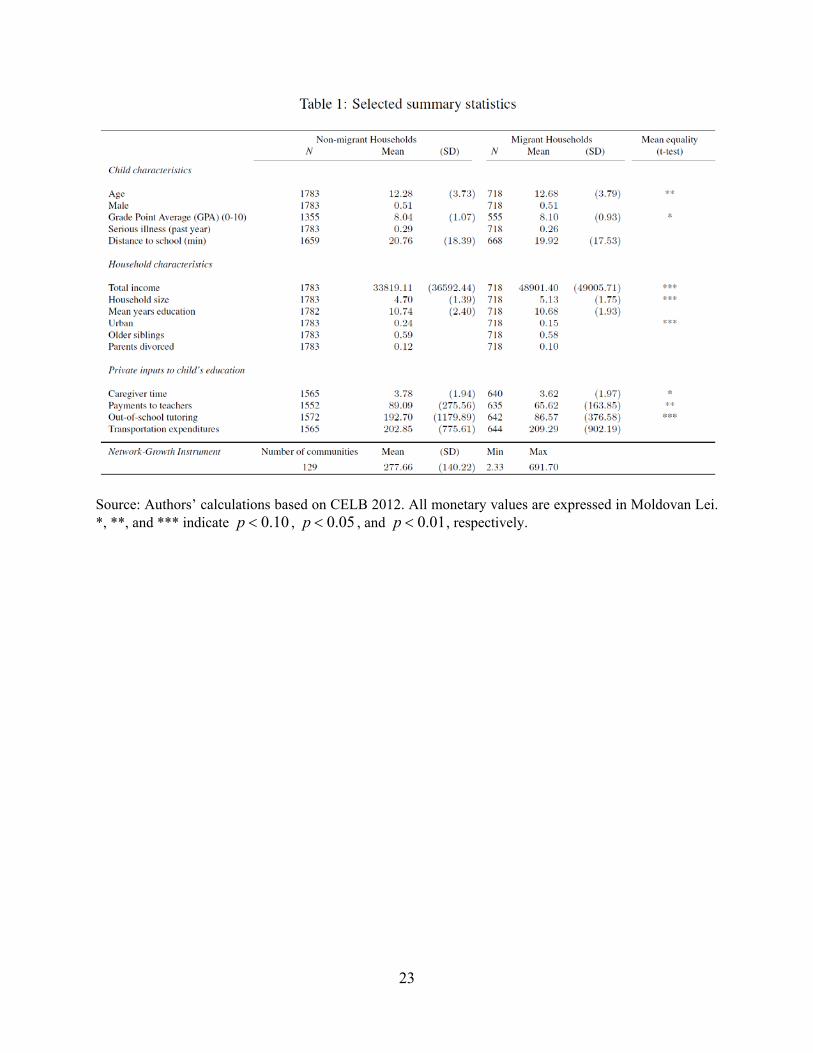
children live in a migrant household (table 1).14 The average student from migrant households is

12.6 years old, five months more than her non-migrant peer. Before accounting for selection into

migration, the average grade (GPA) is 0.06 points higher for children in migrant households.

Migrant families are slightly larger on average and more likely to come from rural areas. Despite

this, their average total income and average per capita income are significantly higher than those

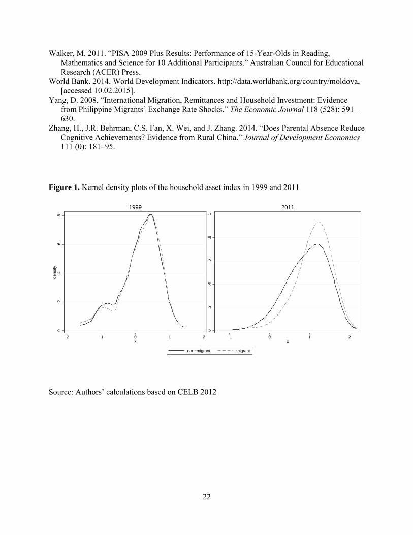
of non-migrants.15 Figure 1 also reflects the underlying effect of migration, showing no

difference in assets in 1999 but significantly higher assets for migrant families in 2011.16

12. The main caregiver is the person responsible for nutrition, health, and schooling of a child at the time of the

survey. 13. In addition, there is a residual category of “other expenditure” for which we find statistically insignificant

effects. 14. Our dataset does not allow us to compare the differences between migrant households with and without

children. Comparisons to other representative data (details on request) reveal that, in households with children, female migration is on average less common. The education level and gender composition do not differ markedly.

15. In reality, the difference could be even wider since migrant households systematically underreport their received remittances and other sources of income (Akee and Kapur 2012).

16. The asset indexes were constructed by a weighted-sum of the following items: (i.) number of cars, motorcycles, bicycles, washing machines, refrigerators, radios, TVs, computers, and cell phones; (ii.) existence of working phone landline and internet access; and (iii.) number of rooms in the house. For 1999, the last three items were excluded due to a large number of missing values. The weights for the index were obtained from a principal

9

Households in our sample report positive payments to teachers for about 37% of all school-

age children.17 Payments to teachers typically vary from 5–40 USD per child per year, which is

substantial given that public expenditure for teaching materials per pupil is about 30 USD per

year, and wage bills per pupil are about 300 USD per year (cf. appendix S.1 and table S.2). In

contrast, households only report tutoring expenses for approximately 10% of children (cf. figure

S.1). Despite higher income, both per child informal payments to teachers and tutoring expenses

are significantly lower in migrant households compared to non-migrant ones. For transportation

expenditure there is no such difference. The differences in informal payments and tutoring are

mostly driven by more migrant households reporting zero payments (not refusals or “don’t

know” answers) rather than by smaller positive expenses. This is not only evident at the

individual level but also results in a strong negative correlation at the community-level between

the share of migrant households and the share of respondents reporting payments to teachers

(table 2: panel A, column 1).18 The slope of the regression line is approximately -0.4, a very high

value that is statistically and economically significant. Note, though, that our data are designed to

be representative at the national but not at the community level. The negative correlation also

holds at the individual level (table 2: panel A, column 2-5).

IV. EMPIRICAL STRATEGY

To analyze whether this strong negative correlation between migration and petty corruption at

the community-level as well as the individual level is indeed closely tied to migration, we

estimate the stylized model:

Migihcs hc ihcs ihcsy X ò (1)

component analysis of the asset list. Dividing the divisible assets by the squared root of household size as an equivalent scaling rule does not change figure 1 in any qualitative way.

17. This figure is remarkably similar to the one reported in the 2013 Global Corruption Barometer: 37% of households in Moldova that came into contact with education authorities paid bribes in the 12 months before the survey (Transparency International 2013). We focus on the likelihood of paying informal fees rather than the values paid since we assume the decision to participate in the informal fee scheme to be the most affected by a change in preferences. Note that we added one LCU to each private expenditure to ensure that the log exists.

18. See figure S.2 for an illustration.

10

where yihcs are private inputs to the education of child i in household h from community c and

school s. We consider three financial inputs (informal payments to teachers, tutoring, and

transport expenditures) and two non-financial inputs if the child is enrolled in school and the

frequency with which the caregiver spends time supporting the child in educational activities.

The main explanatory variable of interest, Mighc is a household-level dummy variable taking the

value one if the child lives in a migrant household and zero otherwise; Xihcs is a vector of child-

and household-level control variables; and ϵihcs is the error term.

Clearly, migrants are not a random population group but rather self-select into migration.

Thus, it can be expected that they systematically exhibit distinct unobservable characteristics

relative to non-migrants that might bias OLS estimates of equation (1). To overcome this

problem, we estimate an instrumental variable approach by two-stage least squares (2SLS).19 Our

instrument for migration status is the interaction between pre-existing migration networks at the

local-level and destination-specific economic conditions. Formally, we use the growth rate of per

capita GDP for each destination country between 2004–2010 and weight it with the share of

migrants that, by 2004, had migrated from the community to that destination.20 The data for the

migrant-destination share at the community level are derived from the 2004 Moldovan Census.21

The variable has already been employed as an instrument for migration in other studies of the

Moldovan context (e.g., Lücke et al. 2012, Böhme et al. 2015). The rationale behind the use of

Network-Growth is twofold. First, migrant networks are known to be very important in

19. The most common approach in the literature is instrumental variable strategies exploiting exogenous

aggregate factors at the origin or destination: past migration rates (McKenzie and Rapoport 2010, Antman 2011, Zhang et al. 2014), financial infrastructure (Calero et al. 2009), and political unrest (Bansak and Chezum 2009) at the origin-level; employment conditions (Antman 2011, Cortes 2015) and exchange rate crises (Yang 2008) at the destination-level.

20. Analytically:

, ,2004 , 1 ,

1 1,2004 ,

migrants GDP GDPNetwork-Growth

population GDP

J Tc j j t j t

cj tc j t

where c is the Moldovan community; 1, 2,3,...,j J is the migration destination countries and t = 2004,

2005, ..., 2010. 21. An advantage of our setting is that migration has been a relatively recent phenomenon in Moldova, and,

thus, there is little scope for the non-migrant population to be influenced over time due to spillovers and long-term confounding developments that might have arisen over time. As a robustness check, we exclude for the analysis the migrant households which already had a migrant in 2004 or before as they might be included in the Census migration rates. The main results do not change qualitatively (available upon request).

11

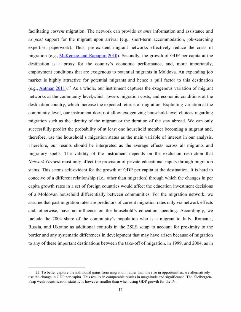
facilitating current migration. The network can provide ex ante information and assistance and

ex post support for the migrant upon arrival (e.g., short-term accommodation, job-searching

expertise, paperwork). Thus, pre-existent migrant networks effectively reduce the costs of

migration (e.g., McKenzie and Rapoport 2010). Secondly, the growth of GDP per capita at the

destination is a proxy for the country’s economic performance, and, more importantly,

employment conditions that are exogenous to potential migrants in Moldova. An expanding job

market is highly attractive for potential migrants and hence a pull factor to this destination

(e.g., Antman 2011).22 As a whole, our instrument captures the exogenous variation of migrant

networks at the community level,which lowers migration costs, and economic conditions at the

destination country, which increase the expected returns of migration. Exploiting variation at the

community level, our instrument does not allow exogenizing household-level choices regarding

migration such as the identity of the migrant or the duration of the stay abroad. We can only

successfully predict the probability of at least one household member becoming a migrant and,

therefore, use the household’s migration status as the main variable of interest in our analysis.

Therefore, our results should be interpreted as the average effects across all migrants and

migratory spells. The validity of the instrument depends on the exclusion restriction that

Network-Growth must only affect the provision of private educational inputs through migration

status. This seems self-evident for the growth of GDP per capita at the destination. It is hard to

conceive of a different relationship (i.e., other than migration) through which the changes in per

capita growth rates in a set of foreign countries would affect the education investment decisions

of a Moldovan household differentially between communities. For the migration network, we

assume that past migration rates are predictors of current migration rates only via network effects

and, otherwise, have no influence on the household’s education spending. Accordingly, we

include the 2004 share of the community’s population who is a migrant to Italy, Romania,

Russia, and Ukraine as additional controls in the 2SLS setup to account for proximity to the

border and any systematic differences in development that may have arisen because of migration

to any of these important destinations between the take-off of migration, in 1999, and 2004, as in

22. To better capture the individual gains from migration, rather than the rise in opportunities, we alternatively

use the change in GDP per capita. This results in comparable results in magnitude and significance. The Kleibergen-Paap weak identification statistic is however smaller than when using GDP growth for the IV.

12

Böhme et al. (2015).23 The IV is not systematically correlated with school expenditures, local

economic conditions as proxied by night lights (Henderson et al. 2012), local infrastructure or

public goods as reported in the community questionnaire. Further, communities with IV values

above and below median values are distributed evenly across the country (figure S.3). Summary

statistics for the IV variable can be found at the bottom of table 1.

V. MAIN RESULTS

The dependent variables of our empirical analysis are the child’s school enrollment status, the

three categories of private education spending - payments to teachers, tutoring expenses,

transportation expenses - and the time spent by the caregiver. The reduced form estimates are

reported in table 2, panel B. The lack of a selection correction results in a statistically significant

correlation between the instrument and school enrollment,24 which indicates better migration

options for those who leave school after the end of compulsory schooling. Correlations between

the instrument and payments to teachers, as well as tutoring expenses, are negative and

statistically significant.25

The first stage IV estimates are reported in panel C of table 2. The Network-Growth-IV is a

positive and highly significant predictor of the household’s migration status. The instrument’s

estimated coefficient implies that a one standard deviation increase in Network-Growth increases

the likelihood of (at least one) household adult member migrating by approximately 14

percentage points. The Kleibergen-Paap rank test rejects underidentification at least at the 5%

significance level in all the 2SLS regressions.

The second stage indicates no statistically significant effect of migration on the enrollment

probability (column 1) as a result of parental migration. Instead, the results indicate a strong

reduction in the likelihood to pay teachers conditional on individual characteristics that is even

more pronounced than the negative correlation in panel A (column 3). For tutoring, we see a

similar negative effect whereas transport expenditure remains unchanged (columns 5 and 7).

Interestingly, the determinants of tutoring are similar to those of paying bribes, supporting the

23. Alternatively using only one control for all migrant shares does not yield different results, but we prefer

keeping to the more conservative ability to control also for different border effects as in that earlier paper. 24. A one standard deviation increase in the instrument implies a 2.5 percentage point reduction in enrollment. 25. See tables S.3, S.4, and S.5 for the point estimates of the control variables for panels B and C.

13

view that tutoring offers a “cleaner” way of making informal payments to teachers. There is

some evidence of caregivers more frequently spending time on the education of their children

(column 8). In order to account for potentially inflated point estimates due to weak IVs, we

provide the conditional likelihood ratio (CLR) confidence region and cluster robust confidence

sets for the respective migration effect at the bottom of the table (Moreira 2009, Mikusheva and

Poi 2006, Finlay and Magnusson 2009). Both methods show that the effect of migration on

informal payments is bounded away from zero even when accounting for weak IVs.26 The results

point to a statistically, as well as economically, significant negative effect of migration on

informal payments.27

The very strong negative correlation, even after rigorously accounting for self-selection,

cannot be the consequence of a mere income effect. At the same time, children’s or parents’

socioeconomic characteristics do not predict petty corruption at the extensive margin very well.

While there is more reporting of payments for older students, girls, and by more educated

parents–one of the core predictors of income–the other controls are statistically insignificant.

Additional analyses yield no evidence of heterogeneous treatment effects by age, yet this is

partly due to imprecise estimates in small subsamples (table S.8).

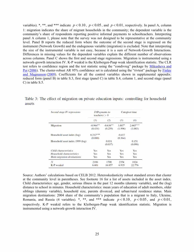
Our main results are not explained by differences in household wealth (proxied by a

household asset index, table 3). Contemporaneous assets are endogenous to migration and, in

fact, constitute one of the main expected transmission channels of migration on education inputs

(column 1 and 3). Pre-migration differences in wealth across households (columns 2 and 4)

should not and do not have any impact on the second stage migration coefficient. To sum up, our

finding on bribes can neither be explained by wealth differences across migrant and non-migrant

households nor by the income effect of remittances.

Regardless of this, the income effect of migration matters by improving families’ ability to

keep children in school. Whereas over 50% of non-migrant parents report barriers that will

prevent the child from achieving the caregiver’s desired level of education this is the case only

for 35% of migrant parents (table S.9: panel A). The modal reason, a lack of finances, is cited by

26. In addition, alternative estimates obtained from an IV probit estimation can be found in table S.6 for comparison.

27. Table S.7 presents OLS estimates for the same set of covariates. Due to the inclusion of a selection correction, covariates such as household size that are predictive of migration but not of informal payments pick up the correlation between migration and informal payments to teachers. The lack of a selection correction also results in statistically significant positive effects on transport expenditure, which are explained by higher available income as additional results show (available upon request).

14

over 80% of caregivers in either group. Migration reduces barriers in general and financial

barriers in particular (table S.9: panel B). The income effect in education is thus strong, in stark

contrast with its effect on petty corruption.

As a supporting ad hoc assessment of the mechanism, log remittances received by the

household can be used in place of the migration dummy as the endogenous variable (results

available on request). In this case, no more significant correlation between the endogenous

variable and informal payment is found in the second stage, which may be taken as tentative

evidence that variation from the instrument does not affect bribe-paying through the remittance

channel. Even though one has to be careful interpreting such evidence because it is no longer a

valid IV approach, this may be interpreted as suggesting that, instead of remittances, other

aspects of migration are likely to be the source of the bribe-reducing effect. In line with other

research, one might hypothesize that the negative coefficient of migration is explained by a

lower willingness to bribe officials in the education system. This could be due to former

migrants’ own likelihood of bribing teachers or through social remittances (cf. Ivlevs and

King 2014, Barsbai et al. forthcoming). Irrespectively of whether it is the migrants themselves or

their families who decrease bribe-paying, our finding is promising from a normative point of

view. From an economic standpoint, the money not given to teachers as informal “service fees”

or “presents” (i.e., for rent-seeking) could be used more productively on other household

expenses and would stop distorting incentives for teachers and students. The emerging picture is

thus a reduction in bribes and a simultaneous increase in the frequency of parental involvement

in children’s education due to migration. In the next section, possible transmission channels will

be discussed in more detail.

VI. TRANSMISSION CHANNELS AND ROBUSTNESS

According to the community leaders interviewed in the survey, the most widely perceived

constraint to school quality is not a scarcity of staff but of other inputs, such as teaching

materials or utilities (table S.10). Parental education inputs could be affected by the public

funding situation of local schools, causing omitted variable bias.28 Thus, we match our household

data with administrative school-level expenditure data from an open budget initiative of the

28. Private educational spending responds to public funding, see for example Houtenville and Conway (2008).

15

World Bank (BOOST) to ensure that the instrument is not picking up community-level variation

in the supply of public education. Matching both datasets is imperfect because the availability of

the budget data was not anticipated at the time of the household survey (see appendix S.1 for a

detailed description of the data and matching procedure). We include the school-level executed

budget in several expenditure categories as additional explanatory variables.29 The strong

negative effect on bribes remains even after adding the additional controls, which approximately

halves the sample size.30 Schools’ wage bills, which closely correspond to the schoolteachers-

per-pupil ratio (cf. figure S.4), teaching material and schools’ maintenance funds are not

significantly correlated with household educational expenditures (table S.11: columns 1-6). By

contrast, schools’ expenditures on utilities and transports, where community leaders often report

lacking funds, exhibit signs of substitutability of private and public expenditure. There is also

some tentative evidence of substitution between the parental investment of time and the time

teachers could allocate to individual children (column 7).31

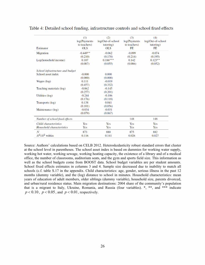
The strong correlation between migration and informal payments to teachers is also robust

when controlling for an index of infrastructural quality of the school (table 4: column 1). We

furthermore tested whether the migration-induced reduction in informal payments is lower in

worse-funded schools where informal payments may be less controversial but did not find any

robust differences (results available upon request). Sending students to schools with funding for

school buses and attending a more distant school, both of which proxy secondary and advanced

secondary schools that cover larger areas, correlate positively (although statistically

insignificantly) with informal payments. Using school fixed-effect regressions to compare

students within schools, we find that better off parents pay more to teachers and buy more

tutoring from their children’s teachers (table 4: columns 3 and 4).32 This underscores the

importance of the income effect. The migration coefficient is negative but insignificant,

suggesting that much of the variation associated with migration occurs at the school level. This

fits well our discussions with Moldovan experts, who stated that the payments to teachers that

29. We do not find evidence that they are systematically correlated with migration. 30. The first-stage estimates are reported in column 2 of table S.4. 31 Table S.12 provides OLS results when the sample is split by migration status. The negative coefficient on the

teacher-pupil ratio (proxied by wages per pupil) is similar for both migrant and non-migrant households, although statistically insignificant for the former.

32. Note that migration as a major source of income inequality is not exogenized here due to a lack of a valid within-community IV.

16

are collected by informal parental committees can quickly stop completely once a few parents

refuse to pay them - an effect that often occurs in public-good settings if punishment is weak

(cf. Fehr and Gächter 2000). In line with our expert discussions, we thus interpret the migration

effects as quickly spilling over within schools.33

To ensure that our results are not driven by local heterogeneity across communities rather

than migration, we add a within-community dimension to the original IV’s community-level

variation. We interact the network-growth IV with the household’s mean years of education

since more educated households can be expected to be better able to respond to the growth-pull

mechanism approximated by our IV. The new variable is positively related with migration and

statistically significant at the 1% level. The estimated effect of migration on payments to

teachers is almost identical to our main estimates (table S.13).

Two motivations for ceasing bribe-paying are plausible: (i) migrant parents being generally

less tolerant of corruption due to their experience abroad; and (ii) migrant parents demanding

actual cognitive achievement instead of good grades because they have witnessed the

unimportance of Moldovan certificates relative to actual skills for success abroad. A full 96% of

caregivers replied that education was important to be successful abroad. Yet, there is no

significant reduction in the perceived quality of children’s individual schools (table S.14).34 This

gives us confidence that our results are not driven by differences in the cost-benefit analysis of

the Moldovan school system between non-migrant and migrant households.

In order to provide some evidence of robustness as well as external validity of our study, we

draw on another, less detailed, dataset to show that a similar negative correlation of migration

and bribe paying exists also in data independent of ours. The so called Barometer of Public

Opinion of Moldova’s Institute for Public Policy, a well-regarded biannual survey which collects

individuals’ opinions on a wide range of topics regarding politics, values, and related issues in

Moldova, covered informal payments to authorities and migration status in the April 2013

survey.35 Those individuals with migration experience to the West were more likely to have had

contact with the justice system and were more likely to have been asked for bribes for the

33. There is no statistically significant correlation between any school budget variable and the migration share of pupils in the household survey. Also, if migrant parents were planning to send their children abroad and therefore stopped paying local teachers, there should be strong differences within schools.

34. Alternatively, the main effects of migration on the provision of educational inputs remain unchanged after including the perceived school quality variable as an additional control (available upon request).

35. The sample contains 1100 individuals from 76 communities and is nationally representative of the adult population. All results are available upon request.

17

solution of their problem. Conditional on reporting not paying a bribe, people with any

experience of migrating and especially the typically more wealthy migrants to the West were

more likely to have been asked to pay informal fees than those without migration experience

(odds ratio: 3.6 times). Individuals with migration experience thus seem to be less likely to pay

bribes under a given level of pressure to do so.36

Finally, our results could be driven by the migration-induced change in the identity of the

child’s caregiver, for example, reflecting that non-parental caregivers (e.g., grandparents,

siblings, aunts, or uncles) have less involvement in (or knowledge of) the education system and

are, therefore, less likely to bribe teachers. They may also have lower opportunity costs of time

and may therefore spend more time on the child’s education. To rule out this mechanism we re-

estimate the main results while excluding all children with caregivers who are not one of their

biological parents (table S.15). The slightly, but not significantly, larger coefficients of migration

provide strong evidence that our results are not driven by caregiver change. Our results are

furthermore robust to alternative but similar definitions of the migration dummy (e.g., who

migrates or how long migration spells have to be). We also find no evidence that our effect is

driven by caregivers who are return migrants.37 More generally, including a dummy variable for

return migrant households (i.e., those households with at least one return migrant but no current

migrants) does not affect the migration coefficient in our educational input IV regressions.

Return migration itself has a negative coefficient which is smaller in absolute magnitude than the

(current) migration estimate, but statistically insignificant (available upon request). Note that

correcting for self-selection into return migration lies beyond the scope of this paper.

Despite controlling for households’ mean years of education in all regressions, it could still

be possible that households were sorted on unobserved ability within Moldova. In that case, the

size of the 2004 network could be correlated with families’ unobservable skills. In the Moldovan

context, this hypothesis is very unlikely. In Soviet times, internal migration was highly restricted

and centralized. Highly skilled individuals were not only concentrated in the main cities, where

tertiary education was available, but were often deployed as state bureaucrats to agricultural or

36. Our instrumental variable strategy does not allow us to identify destination specific effects. Therefore, our

results are the average migration effect across all destinations, not just Western countries. If the effect is entirely driven by migration to the West, where corruption is far less common than in Moldova, then our 2SLS estimates are a lower bound for the true Western migration effect.

37. We define a return migrant as an adult that spent more than three months abroad in one single spell since 1999 but is no longer a migrant at the time of the survey.

18

industrial projects all over the country, especially the countryside. After the collapse of the

Soviet Union, there has not been much internal migration. To corroborate our arguments, we re-

run our main specifications excluding children living in the two cities, Chişinău and Bălţi, that

exert the main pull effect internally. Our results remain fully robust throughout (available upon

request).

As seen above, our main results are robust to a host of alternative explanations. If not paying

bribes, however, had dire consequences for the children’s educational performance, lower

corruption might not be in their best interest. We therefore estimate the effects of migration on

students’ grade point average (GPA) (table S.16). Throughout the different specifications,

payments to teachers remain insignificant. In addition, and in line with the literature, we find a

negative correlation between migration and the GPA that is partly compensated by household

wealth. This underlines that most of the informal payments may not be directly meant to improve

grades relative to classmates but rather operate as illicit user fees or per capita taxes. If their

payment ceases, students on average do not suffer worse grades. However, students who, relative

to their classmates, receive extra attention from teachers due to tutoring (which are partly mere

bribes), do better gradewise. Also, many Moldovans suggest that bribing of teachers for grades is

not effective anyway because students study less hard if they expect to receive higher scores.

Another possibility is that deviating from the common situation of paying bribes has no adverse

effects, especially as standardized tests are increasingly used in the most important exams with

the deliberate aim of fighting corruption in education.

VII. CONCLUSION

In this paper, we analyze the effect of emigration on petty corruption in education, in particular

on informal payments to teachers. Such payments are typically understood to have a dual

motivation: fundraising for maintenance of schools as well as supplementing teachers’ wages to

increase their motivation and/or to focus their attention on individual children. We use the

interaction between migrant networks and economic growth at the destination as an instrumental

variable for the household’s migration status in order to control for selection into migration.

Using this IV approach, we document a reduction in informal payments to teachers. This

aggregate migration effect consists, among others, of a non-negative income effect that is

19

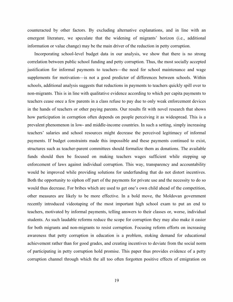
counteracted by other factors. By excluding alternative explanations, and in line with an

emergent literature, we speculate that the widening of migrants’ horizon (i.e., additional

information or value change) may be the main driver of the reduction in petty corruption.

Incorporating school-level budget data in our analysis, we show that there is no strong

correlation between public school funding and petty corruption. Thus, the most socially accepted

justification for informal payments to teachers—the need for school maintenance and wage

supplements for motivation—is not a good predictor of differences between schools. Within

schools, additional analysis suggests that reductions in payments to teachers quickly spill over to

non-migrants. This is in line with qualitative evidence according to which per capita payments to

teachers cease once a few parents in a class refuse to pay due to only weak enforcement devices

in the hands of teachers or other paying parents. Our results fit with novel research that shows

how participation in corruption often depends on people perceiving it as widespread. This is a

prevalent phenomenon in low- and middle-income countries. In such a setting, simply increasing

teachers’ salaries and school resources might decrease the perceived legitimacy of informal

payments. If budget constraints made this impossible and these payments continued to exist,

structures such as teacher-parent committees should formalize them as donations. The available

funds should then be focused on making teachers wages sufficient while stepping up

enforcement of laws against individual corruption. This way, transparency and accountability

would be improved while providing solutions for underfunding that do not distort incentives.

Both the opportunity to siphon off part of the payments for private use and the necessity to do so

would thus decrease. For bribes which are used to get one’s own child ahead of the competition,

other measures are likely to be more effective. In a bold move, the Moldovan government

recently introduced videotaping of the most important high school exam to put an end to

teachers, motivated by informal payments, telling answers to their classes or, worse, individual

students. As such laudable reforms reduce the scope for corruption they may also make it easier

for both migrants and non-migrants to resist corruption. Focusing reform efforts on increasing

awareness that petty corruption in education is a problem, stoking demand for educational

achievement rather than for good grades, and creating incentives to deviate from the social norm

of participating in petty corruption hold promise. This paper thus provides evidence of a petty

corruption channel through which the all too often forgotten positive effects of emigration on

20

origin countries can arise. Future work should seek to more clearly disentangle how such effects

occur and what role the institutional and social contexts play.

REFERENCES

Adams, R.H., and J. Page. 2005. “Do International Migration and Remittances Reduce Poverty in Developing Countries?” World Development 33 (10): 1645–69.

Akee, R., and D. Kapur. 2012. “Remittances and Rashomon.” Working Paper 285, Center for Global Development.

Antman, F.M. 2011. “The Intergenerational Effects of Paternal Migration on Schooling and Work: What Can We Learn from Children’s Time Allocations?” Journal of Development Economics 96 (2): 200–8.

———. 2012. “Gender, Educational Attainment, and the Impact of Parental Migration on Children Left Behind. Journal of Population Economics 25 (4): 1187–214.

Bansak, C., and B. Chezum. 2009. “How do Remittances Affect Human Capital Formation of School-Age Boys and Girls?” The American Economic Review: 145–8.

Barsbai, T., H. Rapoport, A. Steinmayr, and C. Trebesch. Forthcoming. “The Effect of Labor Migration on the Diffusion of Democracy: Evidence from a Former Soviet Republic.” American Economic Journal: Applied Economics.

Batista, C., and P.C. Vicente. 2011. “Do Migrants Improve Governance at Home? Evidence from a Voting Experiment.” The World Bank Economic Review 25 (1): 77–104.

Beine, M., F. Docquier, and M. Schiff. 2013. “International Migration, Transfer of Norms and Home Country Fertility.” Canadian Journal of Economics 46 (4): 1406–30.

Berry, J.W. 1997. “Immigration, Acculturation, and Adaptation.” Applied Psychology 46 (1): 5–34.

Böhme, M., R. Persian, and T. Stöhr. 2015. “Alone But Better Off? Adult Child Migration and Health of Elderly Parents in Moldova.” Journal of Health Economics 39: 211–27.

Böhme, M., T. Stöhr. 2014. “Household Interview Duration Analysis in Capi Survey Management.” Field Methods 26: 390–405.

Borcan, O., M. Lindahl, and A. Mitrut. 2017. “Fighting Corruption in Education: What Works and Who Benefits?” American Economic Journal: Economic Policy 9 (1): 180–209.

Calero, C., A.S. Bedi, and R. Sparrow. 2009. “Remittances, Liquidity Constraints and Human Capital Investments in Ecuador.” World Development 37 (6): 1143–54.

Cameron, L., N. Erkal, L. Gangadharan, and M. Zhang. 2015. “Cultural Integration: Experimental Evidence of Convergence in Immigrants’ Preferences.” Journal of Economic Behavior and Organization 111: 38–58.

Carasciuc, L. 2001. “Corruption and Quality of Governance: the Case of Moldova.” Monograph, Transparency International.

Careja, R., and P. Emmenegger. 2012. “Making Democratic Citizens the Effects of Migration Experience on Political Attitudes in Central and Eastern Europe.” Comparative Political Studies 45 (7): 875–902.

Chauvet, L., and M. Mercier. 2014. “Do Return Migrants Transfer Political Norms to Their Origin Country? Evidence from Mali.” Journal of Comparative Economics 42 (3): 630–51.

21

Corbacho, A., D.W. Gingerich, V. Oliveros, and M. Ruiz-Vega. 2016. “Corruption as a Self-Fulfilling Prophecy: Evidence from a Survey Experiment in Costa Rica. American Journal of Political Science 60 (4): 1077–92.

Cortes, P. 2015. “The Feminization of International Migration and Its Effects on the Children Left Behind: Evidence from the Philippines.” World Development 65: 62–78.

Docquier, F., and H. Rapoport. 2012. “Globalization, Brain Drain, and Development.” Journal of Economic Literature: 681–730.

Dong, B., U. Dulleck, and B. Torgler. 2012. “Conditional Corruption.” Journal of Economic Psychology 33 (3): 609–27.

Emran, M. S., F. Shilpi, and A. Islam. 2013. “Admission Is Free Only If Your Dad Is Rich!: Distributional Effects of Corruption in Schools in Developing Countries.” World Bank Policy Research Working Paper 6671, World Bank.

ESP/NEPC. 2010. Drawing the Line: Parental Informal Payments for Education across Eurasia. Education Support Program (ESP) of the Open Society Institute, Budapest.

Fehr, E., and S. Gächter. 2000. “Cooperation and Punishment in Public Goods Experiments.” The American Economic Review 90 (4): 980–94.

Finlay, K., and L.M. Magnusson. 2009. “Implementing Weak-Instrument Robust Tests for a General Class of Instrumental-Variables Models.” Stata Journal 9 (3): 1–26.

Henderson, J.V., A. Storeygard, and D.N. Weil. 2012. “Measuring Economic Growth from Outer Space.” American Economic Review 102 (2): 994–1028.

Heyneman, S.P., K.H. Anderson, and N. Nuraliyeva. 2008. “The Cost of Corruption in Higher Education.” Comparative Education Review 52 (1): 1–25.

Houtenville, A.J., and K.S. Conway. 2008. “Parental Effort, School Resources, and Student Achievement.” Journal of Human Resources 43 (2): 437–53.

Ivlevs, A., and R.M. King. 2014. “Emigration, Remittances, and Corruption Experience of Those Staying Behind.” IZA Discussion Paper 8521, IZA.

Ivlevs, A. and R. M. King. 2017. "Does emigration reduce corruption?" Public Choice. Lücke, M., T. Omar Mahmoud, and C. Peuker. 2012. “Identifying the Motives of Migrant

Philanthropy.” Working paper no. 1790, Kiel Institute for the World Economy. McKenzie, D., and H. Rapoport. 2010. “Can Migration Reduce Educational Attainment?

Evidence from Mexico.” Journal of Population Economics 24 (4): 1331–58. Mikusheva, A., and B.P. Poi. 2006. “Tests and Confidence Sets With Correct Sive When

Instruments Are Potentially Weak.” Stata Journal 6 (3): 335–47. Moreira, M.J. 2009. “Tests With Correct Size When Instruments Can Be Arbitrarily Weak.”

Journal of Econometrics 152 (2): 131–40. Mountford, A. 1997. “Can A Brain Drain Be Good for Growth in the Source Economy?” Journal

of Development Economics 53 (2): 287–303. MPC. 2013. “Migration Policy Centre: Migration Profile Moldova.” Report. Osipian, A.L. 2009. “Corruption Hierarchies in Higher Education in the Former Soviet Bloc.”

International Journal of Educational Development 29 (3): 321–30. Spilimbergo, A. 2009. “Democracy and Foreign Education.” American Economic Review 99 (1):

528–43. Transparency International. 2013. Global Corruption Barometer: Moldova.

https://www.transparency.org/gcb2013/country/?country=moldova, [accessed 10.06.2015].

22

Walker, M. 2011. “PISA 2009 Plus Results: Performance of 15-Year-Olds in Reading, Mathematics and Science for 10 Additional Participants.” Australian Council for Educational Research (ACER) Press.

World Bank. 2014. World Development Indicators. http://data.worldbank.org/country/moldova, [accessed 10.02.2015].

Yang, D. 2008. “International Migration, Remittances and Household Investment: Evidence from Philippine Migrants’ Exchange Rate Shocks.” The Economic Journal 118 (528): 591–630.

Zhang, H., J.R. Behrman, C.S. Fan, X. Wei, and J. Zhang. 2014. “Does Parental Absence Reduce Cognitive Achievements? Evidence from Rural China.” Journal of Development Economics 111 (0): 181–95.

Figure 1. Kernel density plots of the household asset index in 1999 and 2011

0.2

.4.6

.8de

nsity

−2 −1 0 1 2x

non−migrant migrant

19990

.2.4

.6.8

1

−1 0 1 2x

non−migrant migrant

2011

Source: Authors’ calculations based on CELB 2012

23

Source: Authors’ calculations based on CELB 2012. All monetary values are expressed in Moldovan Lei. *, **, and *** indicate 0.10p , 0.05p , and 0.01p , respectively.

24

Source: Authors’ calculations based on CELB 2012. Standard errors in parentheses. Panel A uses heteroskedasticity-robust standard errors throughout. Panels B and C use heteroskedasticity-robust standard errors that cluster at the community level. All models include a constant. Child characteristics: age, gender, serious illness in the past 12 months (dummy variable), and the (log) distance to school in minutes. Household characteristics: mean years of education of adult members, older siblings (dummy variable), household size, parents divorced, and urban/rural residence status. Main migration destinations: 2004 share of the community’s population that is a migrant to Italy, Ukraine, Romania, and Russia (four

25

variables). *, **, and *** indicate 0.10p , 0.05p , and 0.01p , respectively. In panel A, column 1: migration indicates the share of migrant households in the community; the dependent variable is the community’s share of respondents reporting positive informal payments to schoolteachers. Interpreting panel A column 1, please note that the survey was not designed to be representative at the community level. Panel B reports the reduced form where the outcome of the second stage is regressed on the instrument (Network Growth) and the endogenous variable (migration) is excluded. Note that interpreting the size of the instrumental variable is not easy, because it is a sum of Network-Growth Interactions. Differences in missing values for the dependent variables explain the different number of observations across columns. Panel C shows the first and second stage regressions. Migration is instrumented using a network-growth interaction IV. K-P weakid is the Kleibergen-Paap weak identification statistic. The CLR test refers to confidence region and the test statistic using the “condivreg” package by Mikusheva and Poi (2006). The cluster-robust AR 95% confidence set is calculated using the “rivtest” package by Finlay and Magnusson (2009). Coefficients for all the control variables shown in supplemental appendix: reduced form (panel B) in table S.3, first stage (panel C) in table S.4, column 1, and second stage (panel C) in table S.5.

Source: Authors’ calculations based on CELB 2012. Heteroskedasticity robust standard errors that cluster at the community level in parentheses. See footnote 16 for a list of assets included in the asset index. Child characteristics: age, gender, serious illness in the past 12 months (dummy variable), and the (log) distance to school in minutes. Household characteristics: mean years of education of adult members, older siblings (dummy variable), household size, parents divorced, and urban/rural residence status. Main migration destinations: 2004 share of the community’s population that is a migrant to Italy, Ukraine, Romania, and Russia (4 variables). *, **, and *** indicate 0.10p , 0.05p , and 0.01p , respectively. K-P weakid refers to the Kleibergen-Paap weak identification statistic. Migration is instrumented using a network-growth interaction IV.

26

Source: Authors’ calculations based on CELB 2012. Heteroskedasticity robust standard errors that cluster at the school level in parentheses. The school asset index is based on dummies for working water supply, working hot water, working sewage, working heating capacity, the existence of a library and of a medical office, the number of classrooms, auditorium seats, and the gym and sports field size. This information as well as the school budgets come from BOOST data. School budget variables are per student amounts. School fixed effects estimates in columns 3 and 4. Sample size decreased due to inability to match all schools (c.f. table S.17 in the appendix. Child characteristics: age, gender, serious illness in the past 12 months (dummy variable), and the (log) distance to school in minutes. Household characteristics: mean years of education of adult members, older siblings (dummy variable), household size, parents divorced, and urban/rural residence status. Main migration destinations: 2004 share of the community’s population that is a migrant to Italy, Ukraine, Romania, and Russia (four variables). *, **, and *** indicate

0.10p , 0.05p , and 0.01p , respectively.

Appendix


S.1 Detailed description of school-level data

The data on school-level public expenditures are derived from the World Bank’s Open

Budget Initiative (or BOOST).38 The Moldovan Ministry of Finance provides all budgets

of public organisms at a very disaggregated level and on a yearly basis going back to 2005.

Each item is classified according to source, function and expenditure type. In Moldova,

the financing of public schools is highly decentralized and typically, determined at the

municipality (or rayon) level. We collect all school-level budgets that were executed

during the year 2010 and aggregate expenditures in five categories: 1) staff wages, 2)

teaching materials (also includes food and office supplies), 3) utilities, 4) transportation,

and 5) maintenance (includes small-scale purchases and repairs of physical capital). We

drop all those schools which do not have positive executed expenditures on categories 1),

2) and 3), since they are likely to suffer from severe missing data problems. However, we

allow for zero executed totals on categories 4) and 5), since these are arguably not always

necessary for the core activities of schools.

Finally, we obtain the total number of students for each school from administrative

data of the Moldovan Ministry of Education. In summary, we have complete survey data

for a total of 2,168 school-age children (6-18 years old) from 1,463 households. School

names from the survey and the official records were first matched automatically. In a

second step, we matched strings by hand, thus correcting minor errors such as typos.

Wherever we could certainly establish a link, we then manually entered the school code

for the respective child. In many cases the string variable covering the school name did

not point to a particular school with certainty. Whenever we were less than 100% sure

about the correctness of a match we did not match the respective child’s record. After

matching the survey data with the school-level budgets and number of students, we have

complete data for a sample of 1,158 children from 853 households. Most of the losses in

sample size resulted from not reporting or misreporting the school name in the household

survey and missing executed budget data at the school-level. To a smaller extent, we could

not unambiguously match some school names as reported in the household survey with

their counterparts in the BOOST dataset, for example if parents gave the school name as

i

“liceu <municipality>” but there were several schools of the respective school type in that

municipality.

Table S.17 presents summary statistics of the child-observations successfully matched

across all data sources and of those for which the matching failed. Failure to match is to

some extent random but tends to happen more often in urban areas, where, for example,

a particular part of town has more than one school of a specific kind. As a consequence,

16-18 years old children who attend upper secondary schooling are also disproportion-

ately missing from the matched sample. The reason is that, at higher education levels,

teenagers tend to move away from smaller communities to attend school in more popu-

lous towns, where the chances of ambiguous matches across data sources are higher.39

This pattern also explains why the average distance to school and transportation expen-

ditures are significantly higher for the unmatched sample while average caregiver time is

lower.

For a clearer interpretation of the regression results, Figure S.4 depicts that the school-

level variation on budgets for staff wages is almost completely explained by variation in

the number of teachers employed. The graph plots the values of school expenditures on

wages against the predicted values of a regression of wage spending on the number of

teachers. The red dashed line is the identity line (i.e., y = x). The regression’s R2 is

approximately 98%. Therefore, school budgets for staff wages can be thought of as a

representation of the quantity of schoolteachers.

ii

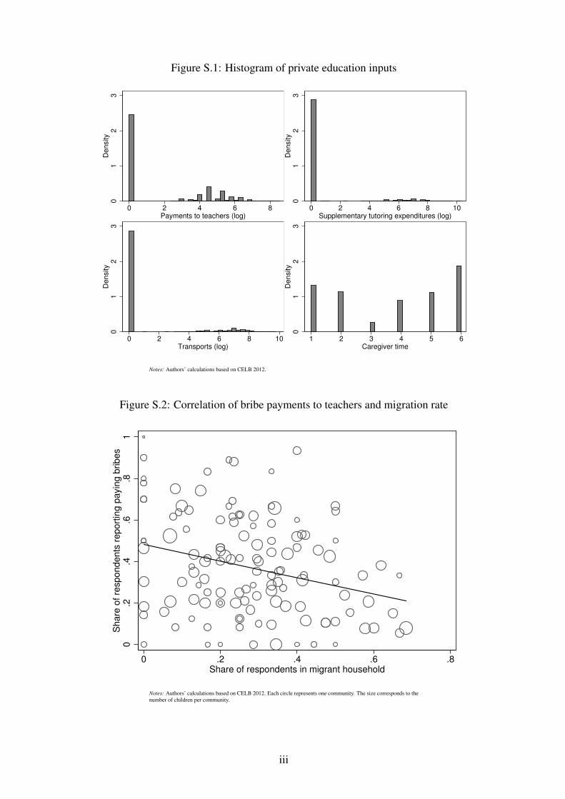
Figure S.1: Histogram of private education inputs

01

23

Density

0 2 4 6 8Payments to teachers (log)

01

23

Density

0 2 4 6 8 10Supplementary tutoring expenditures (log)

01

23

Density

0 2 4 6 8 10Transports (log)

01

23

Density

1 2 3 4 5 6Caregiver time

Notes: Authors’ calculations based on CELB 2012.

Figure S.2: Correlation of bribe payments to teachers and migration rate

0.2

.4.6

.81

Share

of re

spondents

report

ing p

ayin

g b

ribes

0 .2 .4 .6 .8Share of respondents in migrant household

Notes: Authors’ calculations based on CELB 2012. Each circle represents one community. The size corresponds to the

number of children per community.

iii

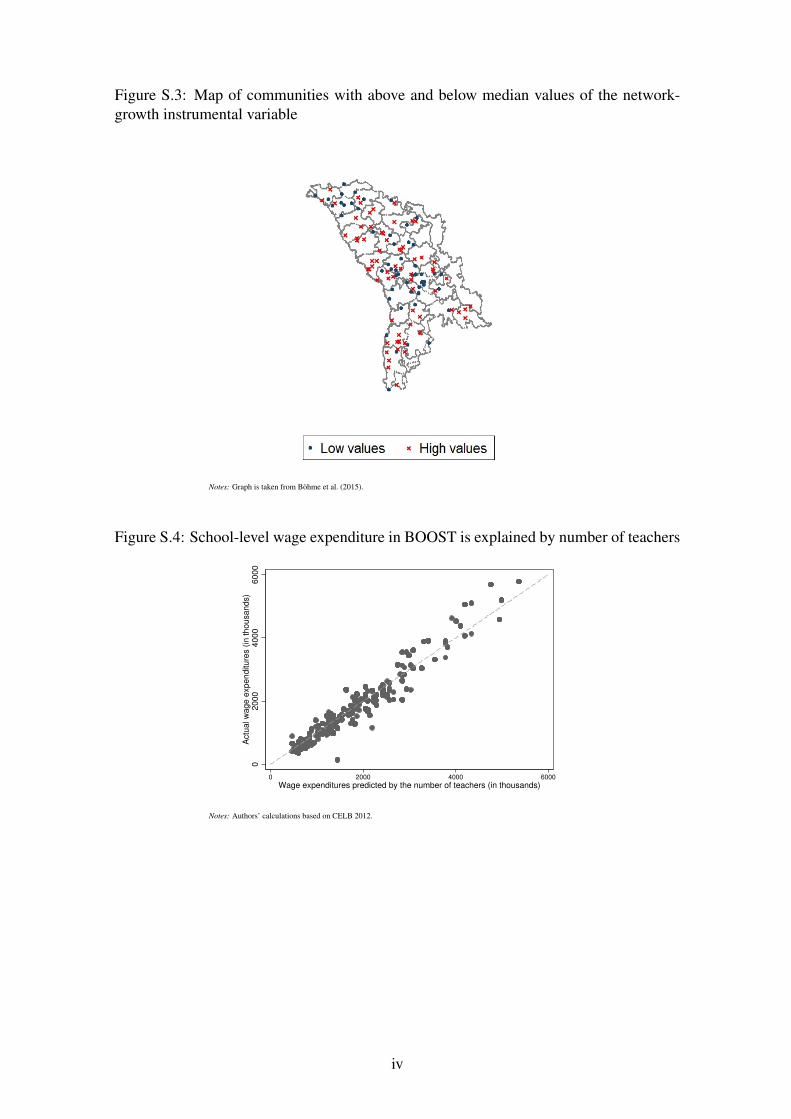
Figure S.3: Map of communities with above and below median values of the network-

growth instrumental variable

Notes: Graph is taken from Böhme et al. (2015).

Figure S.4: School-level wage expenditure in BOOST is explained by number of teachers

02000

6000

4000

Actu

al w

age e

xpenditure

s (

in thousands)

0 2000 4000 6000

Wage expenditures predicted by the number of teachers (in thousands)

Notes: Authors’ calculations based on CELB 2012.

iv

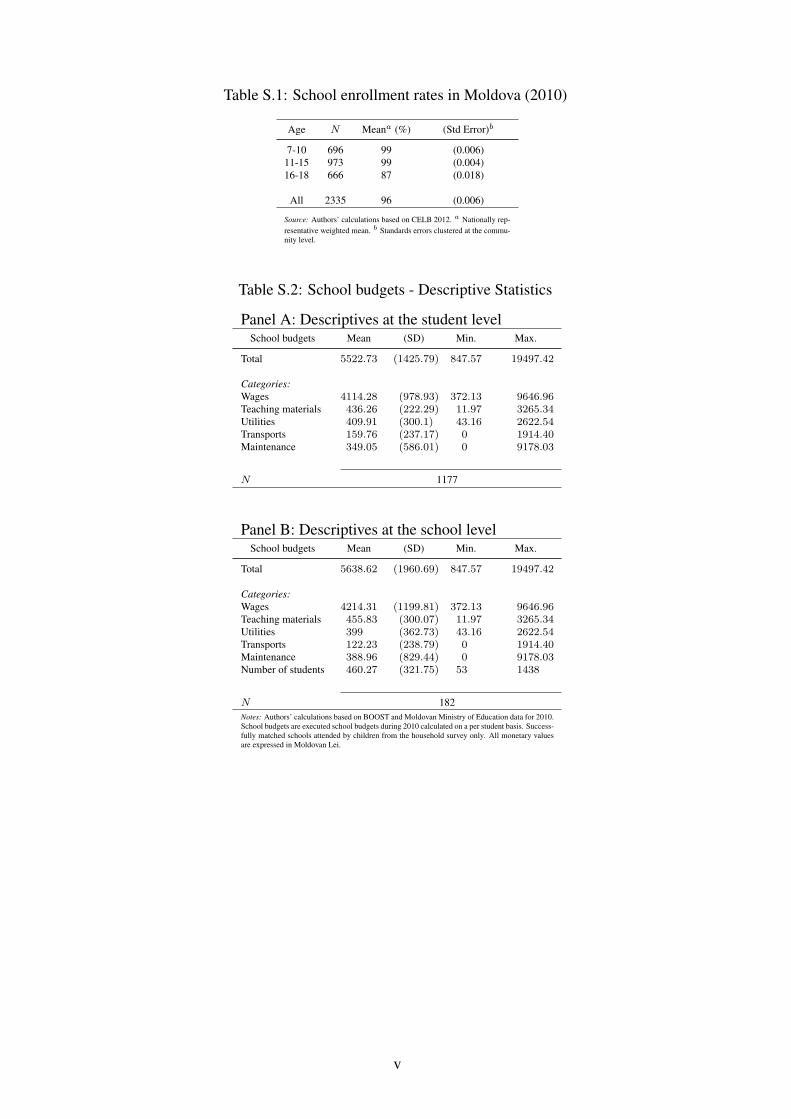
Table S.1: School enrollment rates in Moldova (2010)

Age N Meana (%) (Std Error)b

7-10 696 99 (0.006)

11-15 973 99 (0.004)

16-18 666 87 (0.018)

All 2335 96 (0.006)

Source: Authors’ calculations based on CELB 2012. a Nationally rep-

resentative weighted mean. b Standards errors clustered at the commu-

nity level.

Table S.2: School budgets - Descriptive Statistics

Panel A: Descriptives at the student levelSchool budgets Mean (SD) Min. Max.

Total 5522.73 (1425.79) 847.57 19497.42

Categories:

Wages 4114.28 (978.93) 372.13 9646.96Teaching materials 436.26 (222.29) 11.97 3265.34Utilities 409.91 (300.1) 43.16 2622.54Transports 159.76 (237.17) 0 1914.40Maintenance 349.05 (586.01) 0 9178.03

N 1177

Panel B: Descriptives at the school levelSchool budgets Mean (SD) Min. Max.

Total 5638.62 (1960.69) 847.57 19497.42

Categories:

Wages 4214.31 (1199.81) 372.13 9646.96Teaching materials 455.83 (300.07) 11.97 3265.34Utilities 399 (362.73) 43.16 2622.54Transports 122.23 (238.79) 0 1914.40Maintenance 388.96 (829.44) 0 9178.03Number of students 460.27 (321.75) 53 1438

N 182

Notes: Authors’ calculations based on BOOST and Moldovan Ministry of Education data for 2010.

School budgets are executed school budgets during 2010 calculated on a per student basis. Success-

fully matched schools attended by children from the household survey only. All monetary values

are expressed in Moldovan Lei.

v

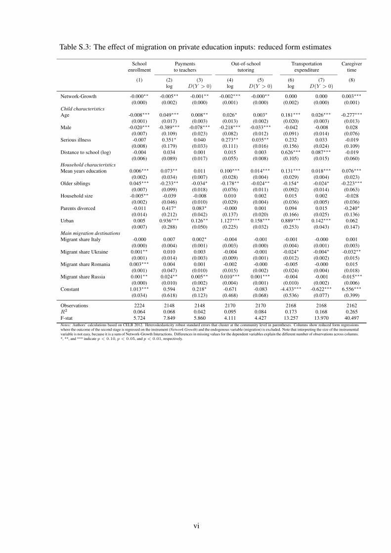
Table S.3: The effect of migration on private education inputs: reduced form estimates

School Payments Out-of-school Transportation Caregiver

enrollment to teachers tutoring expenditure time

(1) (2) (3) (4) (5) (6) (7) (8)

log D(Y > 0) log D(Y > 0) log D(Y > 0)

Network-Growth -0.000∗∗ -0.005∗∗ -0.001∗∗ -0.002∗∗∗ -0.000∗∗ 0.000 0.000 0.003∗∗∗

(0.000) (0.002) (0.000) (0.001) (0.000) (0.002) (0.000) (0.001)

Child characteristics

Age -0.008∗∗∗ 0.049∗∗∗ 0.008∗∗ 0.026∗ 0.003∗ 0.181∗∗∗ 0.026∗∗∗ -0.277∗∗∗

(0.001) (0.017) (0.003) (0.013) (0.002) (0.020) (0.003) (0.013)

Male -0.020∗∗∗ -0.389∗∗∗ -0.078∗∗∗ -0.218∗∗∗ -0.033∗∗∗ -0.042 -0.008 0.028

(0.007) (0.109) (0.023) (0.082) (0.012) (0.091) (0.014) (0.076)

Serious illness -0.007 0.351∗ 0.040 0.273∗∗ 0.035∗∗ 0.232 0.033 -0.019

(0.008) (0.179) (0.033) (0.111) (0.016) (0.156) (0.024) (0.109)

Distance to school (log) -0.004 0.034 0.001 0.015 0.003 0.626∗∗∗ 0.087∗∗∗ -0.019

(0.006) (0.089) (0.017) (0.055) (0.008) (0.105) (0.015) (0.060)

Household characteristics

Mean years education 0.006∗∗∗ 0.073∗∗ 0.011 0.100∗∗∗ 0.014∗∗∗ 0.131∗∗∗ 0.018∗∗∗ 0.076∗∗∗

(0.002) (0.034) (0.007) (0.028) (0.004) (0.029) (0.004) (0.023)

Older siblings 0.045∗∗∗ -0.233∗∗ -0.034∗ -0.178∗∗ -0.024∗∗ -0.154∗ -0.024∗ -0.223∗∗∗

(0.007) (0.099) (0.018) (0.076) (0.011) (0.092) (0.014) (0.063)

Household size -0.005∗∗ -0.039 -0.008 0.010 0.002 0.015 0.002 -0.028

(0.002) (0.046) (0.010) (0.029) (0.004) (0.036) (0.005) (0.036)

Parents divorced -0.011 0.417∗ 0.083∗ -0.000 0.001 0.094 0.015 -0.240∗

(0.014) (0.212) (0.042) (0.137) (0.020) (0.166) (0.025) (0.136)

Urban 0.005 0.936∗∗∗ 0.126∗∗ 1.127∗∗∗ 0.158∗∗∗ 0.889∗∗∗ 0.142∗∗∗ 0.062

(0.007) (0.288) (0.050) (0.225) (0.032) (0.253) (0.043) (0.147)

Main migration destinations

Migrant share Italy -0.000 0.007 0.002∗ -0.004 -0.001 -0.001 -0.000 0.001

(0.000) (0.004) (0.001) (0.003) (0.000) (0.004) (0.001) (0.003)

Migrant share Ukraine 0.001∗∗ 0.010 0.003 -0.004 -0.001 -0.024∗ -0.004∗ -0.032∗∗

(0.001) (0.014) (0.003) (0.009) (0.001) (0.012) (0.002) (0.015)

Migrant share Romania 0.003∗∗∗ 0.004 0.001 -0.002 -0.000 -0.005 -0.000 0.015

(0.001) (0.047) (0.010) (0.015) (0.002) (0.024) (0.004) (0.018)

Migrant share Russia 0.001∗∗ 0.024∗∗ 0.005∗∗ 0.010∗∗∗ 0.001∗∗∗ -0.004 -0.001 -0.015∗∗∗

(0.000) (0.010) (0.002) (0.004) (0.001) (0.010) (0.002) (0.006)

Constant 1.013∗∗∗ 0.594 0.218∗ -0.671 -0.083 -4.433∗∗∗ -0.622∗∗∗ 6.556∗∗∗

(0.034) (0.618) (0.123) (0.468) (0.068) (0.536) (0.077) (0.399)

Observations 2224 2148 2148 2170 2170 2168 2168 2162

R2 0.064 0.068 0.042 0.095 0.084 0.173 0.168 0.265

F-stat 5.724 7.849 5.860 4.111 4.427 13.257 13.970 40.497

Notes: Authors’ calculations based on CELB 2012. Heteroskedasticity robust standard errors that cluster at the community level in parentheses. Columns show reduced form regressions

where the outcome of the second stage is regressed on the instrument (Network Growth) and the endogenous variable (migration) is excluded. Note that interpreting the size of the instrumental

variable is not easy, because it is a sum of Network-Growth Interactions. Differences in missing values for the dependent variables explain the different number of observations across columns.

*, **, and *** indicate p < 0.10, p < 0.05, and p < 0.01, respectively.

vi

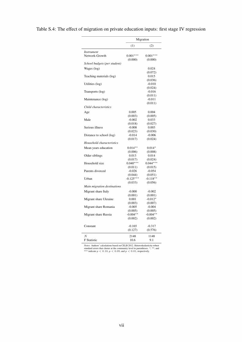
Table S.4: The effect of migration on private education inputs: first stage IV regression

Migration

(1) (2)

Instrument

Network-Growth 0.001∗∗∗ 0.001∗∗∗

(0.000) (0.000)

School budgets (per student)

Wages (log) 0.024

(0.072)

Teaching materials (log) 0.015

(0.036)

Utilities (log) -0.010

(0.024)

Transports (log) -0.016

(0.011)

Maintenance (log) -0.011

(0.011)


Age 0.005 0.004

(0.003) (0.005)

Male -0.002 0.033

(0.018) (0.027)

Serious illness -0.008 0.003

(0.023) (0.030)

Distance to school (log) -0.014 -0.006

(0.017) (0.024)


Mean years education 0.014∗∗ 0.014∗

(0.006) (0.008)

Older siblings 0.013 0.014

(0.017) (0.024)

Household size 0.040∗∗∗ 0.044∗∗∗

(0.011) (0.015)

Parents divorced -0.026 -0.054

(0.044) (0.051)

Urban -0.125∗∗∗ -0.118∗∗

(0.033) (0.056)


Migrant share Italy -0.000 -0.002

(0.001) (0.001)

Migrant share Ukraine 0.001 -0.012∗

(0.003) (0.007)

Migrant share Romania -0.005 -0.004

(0.005) (0.005)

Migrant share Russia -0.004∗∗ -0.004∗∗

(0.002) (0.002)

Constant -0.165 -0.317

(0.127) (0.576)

N 2148 1148

F Statistic 10.6 9.1

Notes: Authors’ calculations based on CELB 2012. Heteroskedasticity robust

standard errors that cluster at the community level in parentheses. *, **, and

*** indicate p < 0.10, p < 0.05, and p < 0.01, respectively.

vii

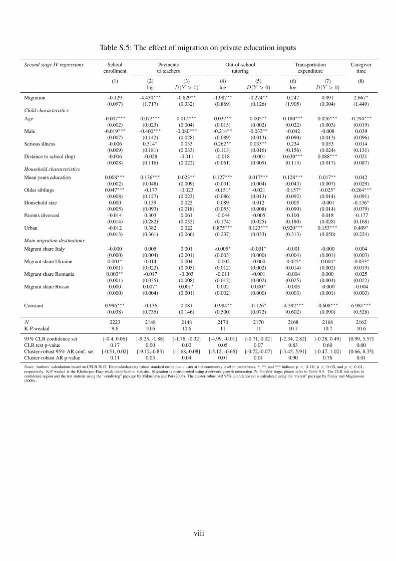
Table S.5: The effect of migration on private education inputs

Second stage IV regressions School Payments Out-of-school Transportation Caregiver


(1) (2) (3) (4) (5) (6) (7) (8)


Migration -0.129 -4.430∗∗∗ -0.829∗∗ -1.987∗∗ -0.274∗∗ 0.247 0.091 2.667∗

(0.097) (1.717) (0.332) (0.869) (0.126) (1.905) (0.304) (1.449)


Age -0.007∗∗∗ 0.072∗∗∗ 0.012∗∗∗ 0.037∗∗ 0.005∗∗ 0.180∗∗∗ 0.026∗∗∗ -0.294∗∗∗

(0.002) (0.023) (0.004) (0.015) (0.002) (0.022) (0.003) (0.019)

Male -0.019∗∗∗ -0.400∗∗∗ -0.080∗∗∗ -0.214∗∗ -0.033∗∗ -0.042 -0.008 0.039

(0.007) (0.142) (0.028) (0.089) (0.013) (0.090) (0.013) (0.096)

Serious illness -0.006 0.314∗ 0.033 0.262∗∗ 0.033∗∗ 0.234 0.033 0.014

(0.009) (0.181) (0.033) (0.113) (0.016) (0.156) (0.024) (0.131)

Distance to school (log) -0.006 -0.028 -0.011 -0.018 -0.001 0.630∗∗∗ 0.088∗∗∗ 0.021

(0.008) (0.116) (0.022) (0.061) (0.009) (0.113) (0.017) (0.087)


Mean years education 0.008∗∗∗ 0.136∗∗∗ 0.023∗∗ 0.127∗∗∗ 0.017∗∗∗ 0.128∗∗∗ 0.017∗∗ 0.042

(0.002) (0.048) (0.009) (0.031) (0.004) (0.043) (0.007) (0.029)

Older siblings 0.047∗∗∗ -0.177 -0.023 -0.151∗ -0.021 -0.157∗ -0.025∗ -0.264∗∗∗

(0.008) (0.127) (0.023) (0.086) (0.013) (0.092) (0.014) (0.091)

Household size 0.000 0.139 0.025 0.089 0.012 0.005 -0.001 -0.136∗

(0.005) (0.093) (0.018) (0.055) (0.008) (0.090) (0.014) (0.079)

Parents divorced -0.014 0.303 0.061 -0.044 -0.005 0.100 0.018 -0.177

(0.014) (0.282) (0.055) (0.174) (0.025) (0.180) (0.028) (0.168)

Urban -0.012 0.382 0.022 0.875∗∗∗ 0.123∗∗∗ 0.920∗∗∗ 0.153∗∗∗ 0.409∗

(0.013) (0.361) (0.066) (0.237) (0.033) (0.313) (0.050) (0.224)


Migrant share Italy -0.000 0.005 0.001 -0.005∗ -0.001∗ -0.001 -0.000 0.004

(0.000) (0.004) (0.001) (0.003) (0.000) (0.004) (0.001) (0.003)

Migrant share Ukraine 0.001∗ 0.014 0.004 -0.002 -0.000 -0.025∗ -0.004∗ -0.033∗

(0.001) (0.022) (0.005) (0.012) (0.002) (0.014) (0.002) (0.019)

Migrant share Romania 0.003∗∗ -0.017 -0.003 -0.011 -0.001 -0.004 0.000 0.025

(0.001) (0.035) (0.008) (0.012) (0.002) (0.025) (0.004) (0.022)

Migrant share Russia 0.000 0.007∗ 0.001∗ 0.002 0.000∗ -0.003 -0.000 -0.004

(0.000) (0.004) (0.001) (0.002) (0.000) (0.003) (0.001) (0.003)

Constant 0.996∗∗∗ -0.136 0.081 -0.984∗∗ -0.126∗ -4.392∗∗∗ -0.608∗∗∗ 6.981∗∗∗

(0.038) (0.735) (0.146) (0.500) (0.072) (0.602) (0.090) (0.528)

N 2223 2148 2148 2170 2170 2168 2168 2162

K-P weakid 9.6 10.6 10.6 11 11 10.7 10.7 10.6

95% CLR confidence set [-0.4, 0.06] [-9.25, -1.88] [-1.76, -0.32] [-4.99, -0.01] [-0.71, 0.02] [-2.34, 2.82] [-0.28, 0.49] [0.99, 5.57]

CLR test p-value 0.17 0.00 0.00 0.05 0.07 0.83 0.60 0.00

Cluster-robust 95% AR conf. set [-0.51, 0.02] [-9.12,-0.83] [-1.68,-0.08] [-5.12, -0.65] [-0.72,-0.07] [-3.45, 5.91] [-0.47, 1.02] [0.66, 8.35]

Cluster-robust AR p-value 0.11 0.03 0.04 0.01 0.01 0.90 0.76 0.01

Notes: Authors’ calculations based on CELB 2012. Heteroskedasticity robust standard errors that cluster at the community level in parentheses. *, **, and *** indicate p < 0.10, p < 0.05, and p < 0.01,

respectively. K-P weakid is the Kleibergen-Paap weak identification statistic. Migration is instrumented using a network-growth interaction IV. For first stage, please refer to Table S.4. The CLR test refers to

confidence region and the test statistic using the “condivreg” package by Mikusheva and Poi (2006). The cluster-robust AR 95% confidence set is calculated using the “rivtest” package by Finlay and Magnusson

(2009).

viii

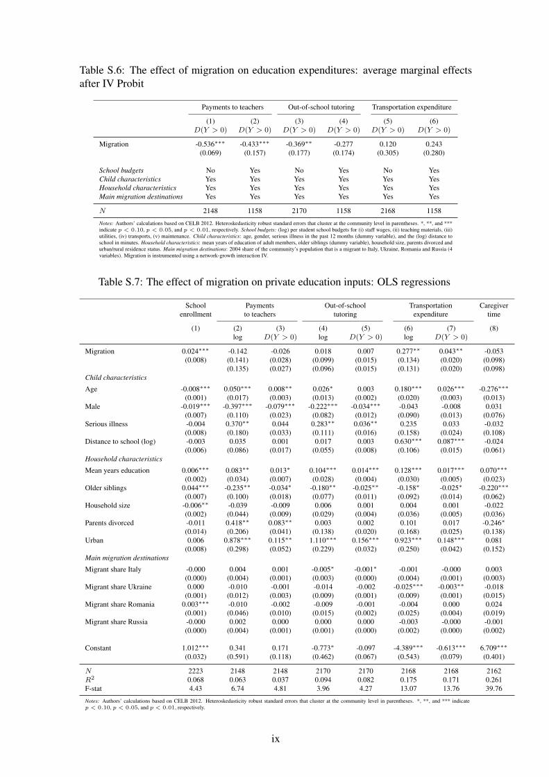
Table S.6: The effect of migration on education expenditures: average marginal effects

after IV Probit

Payments to teachers Out-of-school tutoring Transportation expenditure

(1) (2) (3) (4) (5) (6)

D(Y > 0) D(Y > 0) D(Y > 0) D(Y > 0) D(Y > 0) D(Y > 0)

Migration -0.536∗∗∗ -0.433∗∗∗ -0.369∗∗ -0.277 0.120 0.243

(0.069) (0.157) (0.177) (0.174) (0.305) (0.280)

School budgets No Yes No Yes No Yes

Child characteristics Yes Yes Yes Yes Yes Yes

Household characteristics Yes Yes Yes Yes Yes Yes

Main migration destinations Yes Yes Yes Yes Yes Yes

N 2148 1158 2170 1158 2168 1158

Notes: Authors’ calculations based on CELB 2012. Heteroskedasticity robust standard errors that cluster at the community level in parentheses. *, **, and ***

indicate p < 0.10, p < 0.05, and p < 0.01, respectively. School budgets: (log) per student school budgets for (i) staff wages, (ii) teaching materials, (iii)

utilities, (iv) transports, (v) maintenance. Child characteristics: age, gender, serious illness in the past 12 months (dummy variable), and the (log) distance to

school in minutes. Household characteristics: mean years of education of adult members, older siblings (dummy variable), household size, parents divorced and

urban/rural residence status. Main migration destinations: 2004 share of the community’s population that is a migrant to Italy, Ukraine, Romania and Russia (4

variables). Migration is instrumented using a network-growth interaction IV.

Table S.7: The effect of migration on private education inputs: OLS regressions

School Payments Out-of-school Transportation Caregiver


(1) (2) (3) (4) (5) (6) (7) (8)


Migration 0.024∗∗∗ -0.142 -0.026 0.018 0.007 0.277∗∗ 0.043∗∗ -0.053

(0.008) (0.141) (0.028) (0.099) (0.015) (0.134) (0.020) (0.098)

(0.135) (0.027) (0.096) (0.015) (0.131) (0.020) (0.098)


Age -0.008∗∗∗ 0.050∗∗∗ 0.008∗∗ 0.026∗ 0.003 0.180∗∗∗ 0.026∗∗∗ -0.276∗∗∗

(0.001) (0.017) (0.003) (0.013) (0.002) (0.020) (0.003) (0.013)

Male -0.019∗∗∗ -0.397∗∗∗ -0.079∗∗∗ -0.222∗∗∗ -0.034∗∗∗ -0.043 -0.008 0.031

(0.007) (0.110) (0.023) (0.082) (0.012) (0.090) (0.013) (0.076)

Serious illness -0.004 0.370∗∗ 0.044 0.283∗∗ 0.036∗∗ 0.235 0.033 -0.032

(0.008) (0.180) (0.033) (0.111) (0.016) (0.158) (0.024) (0.108)

Distance to school (log) -0.003 0.035 0.001 0.017 0.003 0.630∗∗∗ 0.087∗∗∗ -0.024

(0.006) (0.086) (0.017) (0.055) (0.008) (0.106) (0.015) (0.061)


Mean years education 0.006∗∗∗ 0.083∗∗ 0.013∗ 0.104∗∗∗ 0.014∗∗∗ 0.128∗∗∗ 0.017∗∗∗ 0.070∗∗∗

(0.002) (0.034) (0.007) (0.028) (0.004) (0.030) (0.005) (0.023)

Older siblings 0.044∗∗∗ -0.235∗∗ -0.034∗ -0.180∗∗ -0.025∗∗ -0.158∗ -0.025∗ -0.220∗∗∗

(0.007) (0.100) (0.018) (0.077) (0.011) (0.092) (0.014) (0.062)

Household size -0.006∗∗ -0.039 -0.009 0.006 0.001 0.004 0.001 -0.022

(0.002) (0.044) (0.009) (0.029) (0.004) (0.036) (0.005) (0.036)

Parents divorced -0.011 0.418∗∗ 0.083∗∗ 0.003 0.002 0.101 0.017 -0.246∗

(0.014) (0.206) (0.041) (0.138) (0.020) (0.168) (0.025) (0.138)

Urban 0.006 0.878∗∗∗ 0.115∗∗ 1.110∗∗∗ 0.156∗∗∗ 0.923∗∗∗ 0.148∗∗∗ 0.081

(0.008) (0.298) (0.052) (0.229) (0.032) (0.250) (0.042) (0.152)


Migrant share Italy -0.000 0.004 0.001 -0.005∗ -0.001∗ -0.001 -0.000 0.003

(0.000) (0.004) (0.001) (0.003) (0.000) (0.004) (0.001) (0.003)

Migrant share Ukraine 0.000 -0.010 -0.001 -0.014 -0.002 -0.025∗∗∗ -0.003∗∗ -0.018

(0.001) (0.012) (0.003) (0.009) (0.001) (0.009) (0.001) (0.015)

Migrant share Romania 0.003∗∗∗ -0.010 -0.002 -0.009 -0.001 -0.004 0.000 0.024

(0.001) (0.046) (0.010) (0.015) (0.002) (0.025) (0.004) (0.019)

Migrant share Russia -0.000 0.002 0.000 0.000 0.000 -0.003 -0.000 -0.001

(0.000) (0.004) (0.001) (0.001) (0.000) (0.002) (0.000) (0.002)

Constant 1.012∗∗∗ 0.341 0.171 -0.773∗ -0.097 -4.389∗∗∗ -0.613∗∗∗ 6.709∗∗∗

(0.032) (0.591) (0.118) (0.462) (0.067) (0.543) (0.079) (0.401)

N 2223 2148 2148 2170 2170 2168 2168 2162

R2 0.068 0.063 0.037 0.094 0.082 0.175 0.171 0.261

F-stat 4.43 6.74 4.81 3.96 4.27 13.07 13.76 39.76

Notes: Authors’ calculations based on CELB 2012. Heteroskedasticity robust standard errors that cluster at the community level in parentheses. *, **, and *** indicate

p < 0.10, p < 0.05, and p < 0.01, respectively.

ix

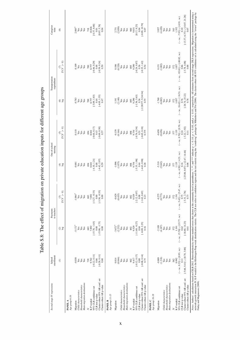
Tab

leS

.8:

The

effe

ctof

mig

rati

on

on

pri

vat

eed

uca

tion

inputs

for

dif

fere

nt

age

gro

ups

Sec

ond

stage

IVre

gre

ssio

ns

Sch

ool

Pay

men

tsO

ut-

of-

school

Tra

nsp

ort

atio

nC

areg

iver

enro

llm

ent

tote

acher

stu

tori

ng

expen

dit

ure

tim

e

(1)

(2)

(3)

(4)

(5)

(6)

(7)

(8)

log

D(Y

>0)

log

D(Y

>0)

log

D(Y

>0)

PA

NE

LA

Age

gro

up

6-1

0

Mig

rati

on

-0.0

30

-5.1

72∗

-1.0

64∗

-0.6

81

-0.1

10

-0.7

83

-0.1

09

2.0

85∗

Chil

dch

ara

cter

isti

csY

esY

esY

esY

esY

esY

esY

esY

es

House

hold

chara

cter

isti

csY

esY

esY

esY

esY

esY

esY

esY

es

Main

mig

rati

on

des

tinati

ons

Yes

Yes

Yes

Yes

Yes

Yes

Yes

Yes

N739

683

683

694

694

700

700

718

K-P

wea

kid

9.7

62

7.8

92

7.8

92

8.8

41

8.8

41

8.7

57

8.7

57

10.8

26

95%

CL

Rco

nfi

den

cese

t[-

0.2

2,0.1

1]

[-15.7

8,-1

.63]

[-3.2

7,-0

.33]

[-4.1

0,1.2

1]

[-0.6

4,0.1

7]

[-3.0

9,1.8

3]

[-0.4

6,0.2

9]

[0.3

7,6.6

8]

CL

Rte

stp-v

alue

0.6

60.0

00.0

00.4

80.4

30.4

40.4

80.0

1

Clu

ster

-robust

95%

AR

conf.

set

[-0.2

8,0.1

1]

[-15.9

8,-1

.75]

[-3.3

0,-0

.35]

[-4.4

2,2.0

7]

[-0.6

9,0.3

0]

[-4.0

5,1.5

5]

[-0.5

9,0.2

4]

[0.0

7,5.7

8]

Clu

ster

-robust

AR

p-v

alue

0.6

80.0

00.0

00.5

90.5

70.4

70.5

00.0

4

PA

NE

LB

Age

gro

up

11-1

5

Mig

rati

on

0.0

14

-3.6

72∗

-0.6

29

-1.0

96

-0.1

39

1.1

91

0.1

86

2.7

51

(0.0

44)

(2.2

32)

(0.4

55)

(1.0

75)

(0.1

64)

(2.1

40)

(0.3

28)

(2.0

50)

Chil

dch

ara

cter

isti

csY

esY

esY

esY

esY

esY

esY

esY

es

House

hold

chara

cter

isti

csY

esY

esY

esY

esY

esY

esY

esY

es

Main

mig

rati

on

des

tinati

ons

Yes

Yes

Yes

Yes

Yes

Yes

Yes

Yes

N902

892

892

898

898

895

895

900

K-P

wea

kid

9.4

17

9.5

29

9.5

29

9.7

54

9.7

54

9.2

90

9.2

90

9.8

31

95%

CL

Rco

nfi

den

cese

t[-

0.1

2,0.1

7]

[-11.6

9,-0

.27]

[-2.1

2,0.0

7]

[-5.3

5,1.9

8]

[-0.7

6,0.3

4]

[-1.5

6,5.6

3]

[-0.2

4,0.8

7]

[0.1

7,9.2

3]

CL

Rte

stp-v

alue

0.8

00.0

40.0

80.4

40.5

10.3

60.3

60.0

4

Clu

ster

-robust

95%

AR

conf.

set

[-0.0

8,0.1

4]

[-8

.89,2.2

5]

[-1.6

2,0.6

5]

[-4.6

3,0.9

0]

[-0.6

5,0.1

8]

[-2.2

8377,9.2

4134]

[-0.3

5,1.4

2]

[-0.0

9,10.7

9]

Clu

ster

-robust

AR

p-v

alue

0.7

50.1

60.2

30.2

80.3

75

0.5

50.5

40.0

7

PA

NE

LC

Age

gro

up

16-1

8

Mig

rati

on

-0.8

89

-2.1

89

-0.2

75

-5.3

19

-0.6

50

-1.7

60

0.1

51

3.9

57

(1.2

18)

(4.1

87)

(0.7

73)

(5.0

42)

(0.6

56)

(6.8

82)

(1.0

02)

(4.4

20)

Chil

dch

ara

cter

isti

csY

esY

esY

esY

esY

esY

esY

esY

es

House

hold

chara

cter

isti

csY

esY

esY

esY

esY

esY

esY

esY

es

Main

mig

rati

on

des

tinati

ons

Yes

Yes

Yes

Yes

Yes

Yes

Yes

Yes

N582

572

572

577

577

572

572

543

K-P

wea

kid

0.9

92

1.1

91

1.1

91

1.1

35

1.1

35

1.0

57

1.0

57

1.3

52

95%

CL

Rco

nfi

den

cese

t(−

∞,0.2

3]∪

[0.9

3,∞

)(−

∞,15.7

0]∪

[15.7

7,∞

)(−

∞,5.4

2]∪

[5.4

7,∞

)(−

∞,4.2

0]∪

[4.2

1,∞

)(−

∞,0.7

0]∪

[0.7

0,∞

)(−

∞,18.4

2]∪

[18.5

1,∞

)(−

∞,-9

3.8

1]∪

[-80.8

2,∞

)(−

∞,-7

.93]∪

[-0.9

1,∞

)

CL

Rte

stp-v

alue

0.1

10.6

20.7

50.1

60.2

40.7

60.8

60.1

0

Clu

ster

-robust

95%

AR

conf.

set

[-5.6

6,0.4

1]∪

[0.7

0,3.8

8]

[-18.6

0,14.2

3]

[-3.3

1,2.7

6]

[-25.0

8,0.0

7]∪

[2.4

7,14.4

4]

[-3.2

2,1.9

2]

[-28.7

4,25.2

2]

[-3.7

8,4.0

8]

[-13.3

7,-

6.3

7]∪

[-0.0

7,21.2

8]

Clu

ster

-robust

AR

p-v

alue

0.6

10.7

30.0

60.1

10.7

80.8

80.0

7

Note

s:A

uth

ors

’ca

lcula

tions

bas

edon

CE

LB

2012.

Het

erosk

edas

tici

tyro

bust

stan

dar

der

rors

that

clust

erat

the

com

munit

yle

vel

inpar

enth

eses

.*,**,an

d***

indic

atep<

0.10

,p<

0.05

,an

dp<

0.01

,re

spec

tivel

y.A

lles

tim

ates

from

seco

nd

stag

e2S

LS

regre

ssio

ns.

Mig

rati

on

isin

stru

men

ted

usi

ng

a

net

work

-gro

wth

inte

ract

ion

IV.

K-P

wea

kid

isth

eK

leib

ergen

-Paa

pw

eak

iden

tifi

cati

on

stat

isti

c.T

he

CL

Rte

stre

fers

toco

nfi

den

cere

gio

nan

dth

ete

stst

atis

tic

usi

ng

the

“condiv

reg”

pac

kag

eby

Mik

ush

eva

and

Poi

(2006).

The

clust

er-r

obust

AR

95%

confi

den

cese

tis

calc

ula

ted

usi

ng

the

“riv

test

”pac

kag

eby

Fin

lay

and

Mag

nuss

on

(2009).

x

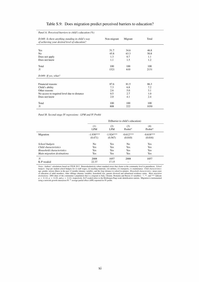
Table S.9: Does migration predict perceived barriers to education?

Panel A: Perceived barriers to child’s education (%)

D.048: Is there anything standing in child’s way

of achieving your desired level of education?

Non-migrant Migrant Total

Yes 51.7 34.6 46.8

No 45.8 63.3 50.8

Does not apply 1.3 0.7 1.1

Does not know 1.1 1.5 1.2

Total 100 100 100

N 1521 610 2131

D.049: If yes, what?

Financial reasons 87.6 81.5 86.3

Child’s ability 7.3 6.8 7.2

Other reasons 2.6 5.0 3.1

No access to required level due to distance 0.5 2.7 1.0

Does not know 2.0 4.1 2.4

Total 100 100 100

N 808 222 1030

Panel B: Second-stage IV regressions - LPM and IV Probit

D(Barrier to child’s education)

(1) (2) (3) (4)

LPM LPM Probita Probita

Migration -1.930*** -1.924*** -0.612*** -0.618***

(0.471) (0.567) (0.010) (0.016)

School budgets No Yes No Yes

Child characteristics Yes Yes Yes Yes

Household characteristics Yes Yes Yes Yes

Main migration destinations Yes Yes Yes Yes

N 2008 1057 2008 1057

K-P weakid 22.37 17.15 – –

Notes: Authors’ calculations based on CELB 2012. Heteroskedasticity robust standard errors that cluster at the community level in parentheses. School

budgets: (log) per student school budgets for (i) staff wages, (ii) teaching materials, (iii) utilities, (iv) transports, (v) maintenance. Child characteristics:

age, gender, serious illness in the past 12 months (dummy variable), and the (log) distance to school in minutes. Household characteristics: mean years

of education of adult members, older siblings (dummy variable), household size, parents divorced and urban/rural residence status. Main migration

destinations: 2004 share of the community’s population that is a migrant to Italy, Ukraine, Romania and Russia (4 variables). *, **, and *** indicate

p < 0.10, p < 0.05, and p < 0.01, respectively. K-P weakid refers to the Kleibergen-Paap weak identification statistic. Migration is instrumented

using a network-growth interaction IV. a average partial effect (APE) reported for IV probit.

xi

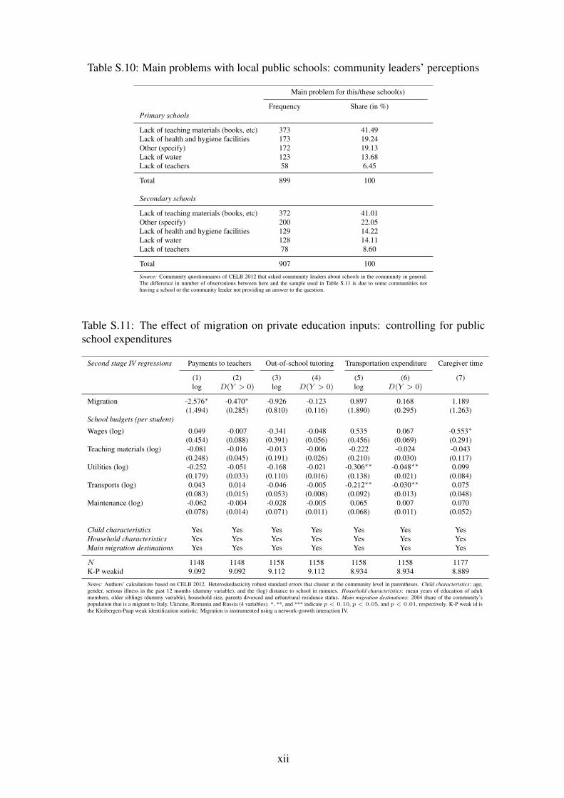
Table S.10: Main problems with local public schools: community leaders’ perceptions

Main problem for this/these school(s)

Frequency Share (in %)

Primary schools

Lack of teaching materials (books, etc) 373 41.49

Lack of health and hygiene facilities 173 19.24

Other (specify) 172 19.13

Lack of water 123 13.68

Lack of teachers 58 6.45

Total 899 100

Secondary schools

Lack of teaching materials (books, etc) 372 41.01

Other (specify) 200 22.05

Lack of health and hygiene facilities 129 14.22

Lack of water 128 14.11

Lack of teachers 78 8.60

Total 907 100

Source: Community questionnaires of CELB 2012 that asked community leaders about schools in the community in general.

The difference in number of observations between here and the sample used in Table S.11 is due to some communities not

having a school or the community leader not providing an answer to the question.

Table S.11: The effect of migration on private education inputs: controlling for public

school expenditures

Second stage IV regressions Payments to teachers Out-of-school tutoring Transportation expenditure Caregiver time

(1) (2) (3) (4) (5) (6) (7)


Migration -2.576∗ -0.470∗ -0.926 -0.123 0.897 0.168 1.189

(1.494) (0.285) (0.810) (0.116) (1.890) (0.295) (1.263)


Wages (log) 0.049 -0.007 -0.341 -0.048 0.535 0.067 -0.553∗

(0.454) (0.088) (0.391) (0.056) (0.456) (0.069) (0.291)

Teaching materials (log) -0.081 -0.016 -0.013 -0.006 -0.222 -0.024 -0.043

(0.248) (0.045) (0.191) (0.026) (0.210) (0.030) (0.117)

Utilities (log) -0.252 -0.051 -0.168 -0.021 -0.306∗∗ -0.048∗∗ 0.099

(0.179) (0.033) (0.110) (0.016) (0.138) (0.021) (0.084)

Transports (log) 0.043 0.014 -0.046 -0.005 -0.212∗∗ -0.030∗∗ 0.075

(0.083) (0.015) (0.053) (0.008) (0.092) (0.013) (0.048)

Maintenance (log) -0.062 -0.004 -0.028 -0.005 0.065 0.007 0.070

(0.078) (0.014) (0.071) (0.011) (0.068) (0.011) (0.052)

Child characteristics Yes Yes Yes Yes Yes Yes Yes

Household characteristics Yes Yes Yes Yes Yes Yes Yes

Main migration destinations Yes Yes Yes Yes Yes Yes Yes

N 1148 1148 1158 1158 1158 1158 1177

K-P weakid 9.092 9.092 9.112 9.112 8.934 8.934 8.889

Notes: Authors’ calculations based on CELB 2012. Heteroskedasticity robust standard errors that cluster at the community level in parentheses. Child characteristics: age,

gender, serious illness in the past 12 months (dummy variable), and the (log) distance to school in minutes. Household characteristics: mean years of education of adult

members, older siblings (dummy variable), household size, parents divorced and urban/rural residence status. Main migration destinations: 2004 share of the community’s

population that is a migrant to Italy, Ukraine, Romania and Russia (4 variables). *, **, and *** indicate p < 0.10, p < 0.05, and p < 0.01, respectively. K-P weak id is

the Kleibergen-Paap weak identification statistic. Migration is instrumented using a network-growth interaction IV.

xii

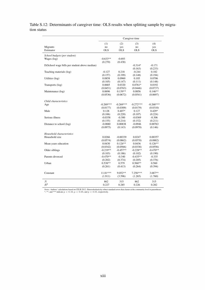
Table S.12: Determinants of caregiver time: OLS results when splitting sample by migra-

tion status

Caregiver time

(1) (2) (3) (4)

Migrants no yes no yes

Estimator OLS OLS OLS OLS


Wages (log) -0.633** -0.693

(0.270) (0.438)

D(School wage bills per student above median) -0.314* -0.171

(0.163) (0.233)

Teaching materials (log) -0.127 0.218 -0.244 0.182

(0.157) (0.199) (0.148) (0.194)

Utilities (log) 0.0858 0.0960 0.105 0.0706

(0.105) (0.147) (0.111) (0.148)

Transports (log) 0.0685 0.0320 0.0761* 0.0192

(0.0451) (0.0763) (0.0446) (0.0737)

Maintenance (log) 0.0696 0.139** 0.0856 0.146**

(0.0536) (0.0672) (0.0541) (0.0697)


Age -0.269*** -0.269*** -0.272*** -0.268***

(0.0177) (0.0309) (0.0179) (0.0310)

Male 0.128 0.407* 0.127 0.429*

(0.106) (0.220) (0.107) (0.224)

Serious illness -0.0358 -0.300 -0.0369 -0.306

(0.155) (0.214) (0.152) (0.211)

Distance to school (log) -0.0880 0.00838 -0.0946 0.00763

(0.0975) (0.143) (0.0970) (0.146)


Household size 0.0266 -0.00339 0.0247 0.00357

(0.0574) (0.0862) (0.0570) (0.0882)

Mean years education 0.0430 0.124** 0.0436 0.126**

(0.0342) (0.0566) (0.0338) (0.0556)

Older siblings -0.219** -0.457** -0.228** -0.470**

(0.103) (0.186) (0.102) (0.190)

Parents divorced -0.470** -0.340 -0.435** -0.335

(0.202) (0.374) (0.205) (0.376)

Urban 0.538** 0.579 0.560** 0.560

(0.261) (0.413) (0.264) (0.394)

Constant 11.81*** 9.052** 7.256*** 3.687**

(1.911) (3.596) (1.265) (1.760)

N 862 315 862 315

R2 0.227 0.285 0.226 0.282

Notes: Authors’ calculations based on CELB 2012. Heteroskedasticity robust standard errors that cluster at the community level in parentheses.

*, **, and *** indicate p < 0.10, p < 0.05, and p < 0.01, respectively.

xiii

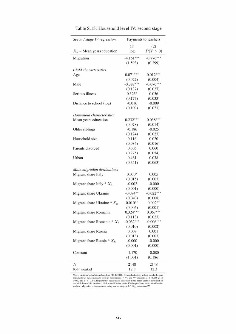
Table S.13: Household level IV: second stage

Second stage IV regression Payments to teachers

(1) (2)

Xh = Mean years education log D(Y > 0)

Migration -4.161∗∗∗ -0.776∗∗∗

(1.593) (0.299)


Age 0.071∗∗∗ 0.012∗∗∗

(0.022) (0.004)

Male -0.382∗∗∗ -0.076∗∗∗

(0.137) (0.027)

Serious illness 0.325∗ 0.036

(0.177) (0.033)


(0.109) (0.021)


Mean years education 0.232∗∗∗ 0.038∗∗∗

(0.078) (0.014)

Older siblings -0.186 -0.025

(0.124) (0.023)

Household size 0.116 0.020

(0.084) (0.016)

Parents divorced 0.305 0.060

(0.275) (0.054)

Urban 0.461 0.038

(0.351) (0.063)


Migrant share Italy 0.030∗ 0.005

(0.015) (0.003)

Migrant share Italy * Xh -0.002 -0.000

(0.001) (0.000)

Migrant share Ukraine -0.094∗∗ -0.022∗∗∗

(0.040) (0.008)

Migrant share Ukraine * Xh 0.010∗∗ 0.002∗∗

(0.005) (0.001)

Migrant share Romania 0.324∗∗∗ 0.067∗∗∗

(0.113) (0.023)

Migrant share Romania * Xh -0.032∗∗∗ -0.006∗∗∗

(0.010) (0.002)

Migrant share Russia 0.008 0.001

(0.013) (0.003)

Migrant share Russia * Xh -0.000 -0.000

(0.001) (0.000)

Constant -1.170 -0.080

(1.001) (0.186)

N 2148 2148

K-P weakid 12.3 12.3

Notes: Authors’ calculations based on CELB 2012. Heteroskedasticity robust standard errors

that cluster at the community level in parentheses. *, **, and *** indicate p < 0.10, p <

0.05, and p < 0.01, respectively. Mean years education is the mean years of education of

the adult household members. K-P weakid refers to the Kleibergen-Paap weak identification

statistic. Migration is instrumented using a network-growth * Xh interaction IV.

xiv

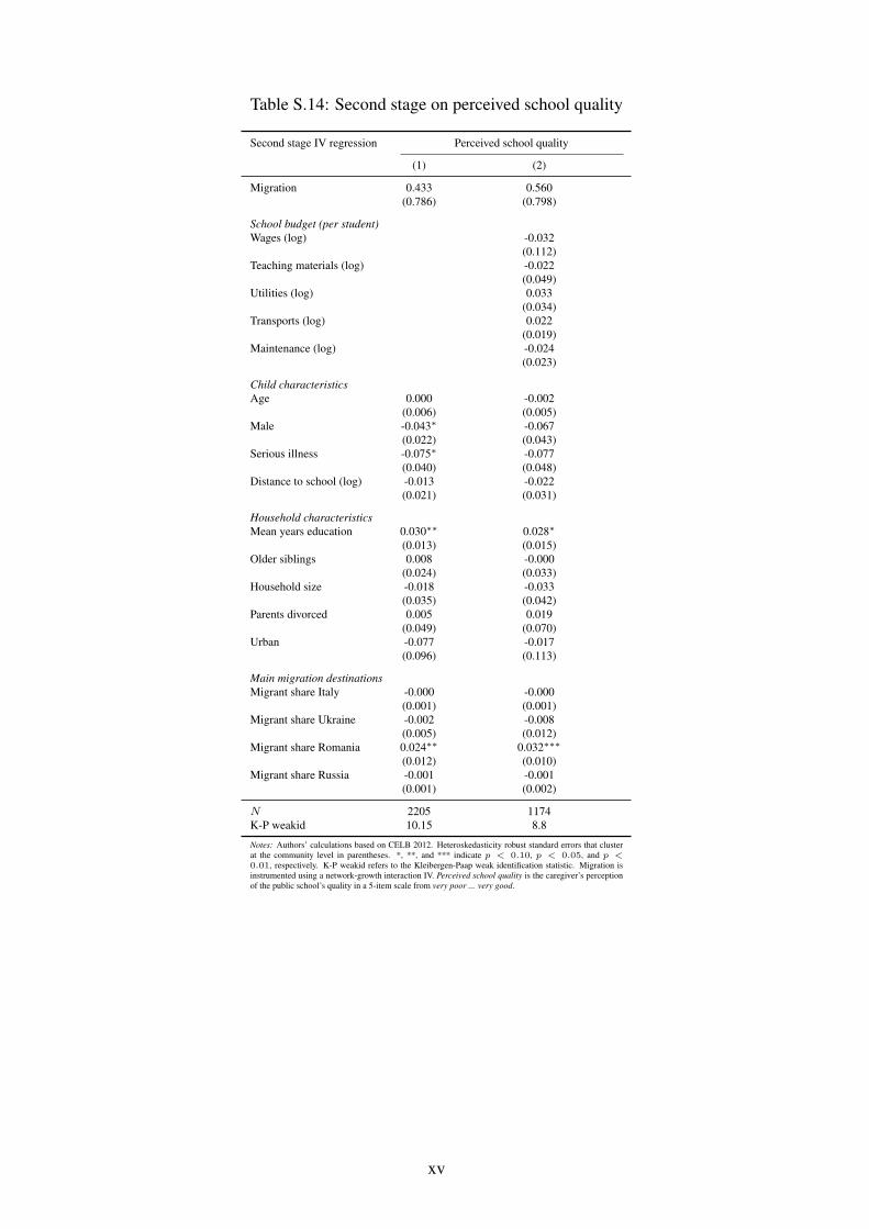
Table S.14: Second stage on perceived school quality

Second stage IV regression Perceived school quality

(1) (2)

Migration 0.433 0.560

(0.786) (0.798)

School budget (per student)

Wages (log) -0.032

(0.112)

Teaching materials (log) -0.022

(0.049)

Utilities (log) 0.033

(0.034)

Transports (log) 0.022

(0.019)

Maintenance (log) -0.024

(0.023)


Age 0.000 -0.002

(0.006) (0.005)

Male -0.043∗ -0.067

(0.022) (0.043)

Serious illness -0.075∗ -0.077

(0.040) (0.048)


(0.021) (0.031)


Mean years education 0.030∗∗ 0.028∗

(0.013) (0.015)

Older siblings 0.008 -0.000

(0.024) (0.033)

Household size -0.018 -0.033

(0.035) (0.042)

Parents divorced 0.005 0.019

(0.049) (0.070)

Urban -0.077 -0.017

(0.096) (0.113)


Migrant share Italy -0.000 -0.000

(0.001) (0.001)

Migrant share Ukraine -0.002 -0.008

(0.005) (0.012)

Migrant share Romania 0.024∗∗ 0.032∗∗∗

(0.012) (0.010)

Migrant share Russia -0.001 -0.001

(0.001) (0.002)

N 2205 1174

K-P weakid 10.15 8.8

Notes: Authors’ calculations based on CELB 2012. Heteroskedasticity robust standard errors that cluster

at the community level in parentheses. *, **, and *** indicate p < 0.10, p < 0.05, and p <

0.01, respectively. K-P weakid refers to the Kleibergen-Paap weak identification statistic. Migration is

instrumented using a network-growth interaction IV. Perceived school quality is the caregiver’s perception

of the public school’s quality in a 5-item scale from very poor ... very good.

xv

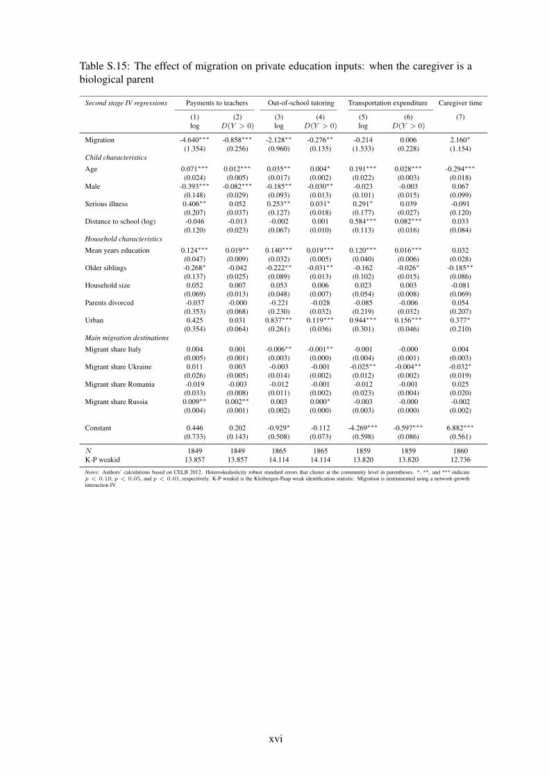
Table S.15: The effect of migration on private education inputs: when the caregiver is a

biological parent

Second stage IV regressions Payments to teachers Out-of-school tutoring Transportation expenditure Caregiver time

(1) (2) (3) (4) (5) (6) (7)


Migration -4.640∗∗∗ -0.858∗∗∗ -2.128∗∗ -0.276∗∗ -0.214 0.006 2.160∗

(1.354) (0.256) (0.960) (0.135) (1.533) (0.228) (1.154)


Age 0.071∗∗∗ 0.012∗∗∗ 0.035∗∗ 0.004∗ 0.191∗∗∗ 0.028∗∗∗ -0.294∗∗∗

(0.024) (0.005) (0.017) (0.002) (0.022) (0.003) (0.018)

Male -0.393∗∗∗ -0.082∗∗∗ -0.185∗∗ -0.030∗∗ -0.023 -0.003 0.067

(0.148) (0.029) (0.093) (0.013) (0.101) (0.015) (0.099)

Serious illness 0.406∗∗ 0.052 0.253∗∗ 0.031∗ 0.291∗ 0.039 -0.091

(0.207) (0.037) (0.127) (0.018) (0.177) (0.027) (0.120)

Distance to school (log) -0.046 -0.013 -0.002 0.001 0.584∗∗∗ 0.082∗∗∗ 0.033

(0.120) (0.023) (0.067) (0.010) (0.113) (0.016) (0.084)


Mean years education 0.124∗∗∗ 0.019∗∗ 0.140∗∗∗ 0.019∗∗∗ 0.120∗∗∗ 0.016∗∗∗ 0.032

(0.047) (0.009) (0.032) (0.005) (0.040) (0.006) (0.028)

Older siblings -0.268∗ -0.042 -0.222∗∗ -0.031∗∗ -0.162 -0.026∗ -0.185∗∗

(0.137) (0.025) (0.089) (0.013) (0.102) (0.015) (0.086)

Household size 0.052 0.007 0.053 0.006 0.023 0.003 -0.081

(0.069) (0.013) (0.048) (0.007) (0.054) (0.008) (0.069)

Parents divorced -0.037 -0.000 -0.221 -0.028 -0.085 -0.006 0.054

(0.353) (0.068) (0.230) (0.032) (0.219) (0.032) (0.207)

Urban 0.425 0.031 0.837∗∗∗ 0.119∗∗∗ 0.944∗∗∗ 0.156∗∗∗ 0.377∗

(0.354) (0.064) (0.261) (0.036) (0.301) (0.046) (0.210)


Migrant share Italy 0.004 0.001 -0.006∗∗ -0.001∗∗ -0.001 -0.000 0.004

(0.005) (0.001) (0.003) (0.000) (0.004) (0.001) (0.003)

Migrant share Ukraine 0.011 0.003 -0.003 -0.001 -0.025∗∗ -0.004∗∗ -0.032∗

(0.026) (0.005) (0.014) (0.002) (0.012) (0.002) (0.019)

Migrant share Romania -0.019 -0.003 -0.012 -0.001 -0.012 -0.001 0.025

(0.033) (0.008) (0.011) (0.002) (0.023) (0.004) (0.020)

Migrant share Russia 0.009∗∗ 0.002∗∗ 0.003 0.000∗ -0.003 -0.000 -0.002

(0.004) (0.001) (0.002) (0.000) (0.003) (0.000) (0.002)

Constant 0.446 0.202 -0.929∗ -0.112 -4.269∗∗∗ -0.597∗∗∗ 6.882∗∗∗

(0.733) (0.143) (0.508) (0.073) (0.598) (0.086) (0.561)

N 1849 1849 1865 1865 1859 1859 1860

K-P weakid 13.857 13.857 14.114 14.114 13.820 13.820 12.736

Notes: Authors’ calculations based on CELB 2012. Heteroskedasticity robust standard errors that cluster at the community level in parentheses. *, **, and *** indicate

p < 0.10, p < 0.05, and p < 0.01, respectively. K-P weakid is the Kleibergen-Paap weak identification statistic. Migration is instrumented using a network-growth

interaction IV.

xvi

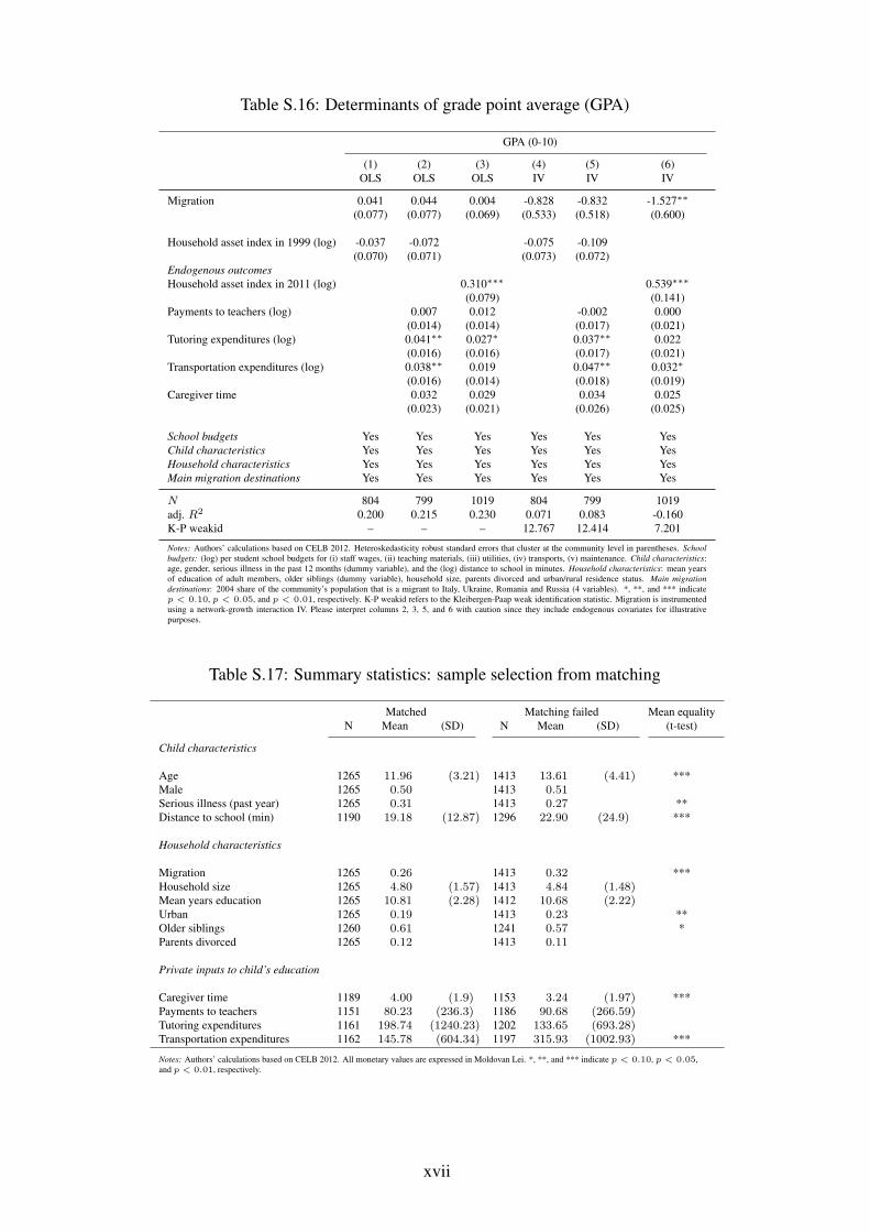
Table S.16: Determinants of grade point average (GPA)

GPA (0-10)

(1) (2) (3) (4) (5) (6)

OLS OLS OLS IV IV IV

Migration 0.041 0.044 0.004 -0.828 -0.832 -1.527∗∗

(0.077) (0.077) (0.069) (0.533) (0.518) (0.600)

Household asset index in 1999 (log) -0.037 -0.072 -0.075 -0.109

(0.070) (0.071) (0.073) (0.072)

Endogenous outcomes

Household asset index in 2011 (log) 0.310∗∗∗ 0.539∗∗∗

(0.079) (0.141)

Payments to teachers (log) 0.007 0.012 -0.002 0.000

(0.014) (0.014) (0.017) (0.021)

Tutoring expenditures (log) 0.041∗∗ 0.027∗ 0.037∗∗ 0.022

(0.016) (0.016) (0.017) (0.021)

Transportation expenditures (log) 0.038∗∗ 0.019 0.047∗∗ 0.032∗

(0.016) (0.014) (0.018) (0.019)

Caregiver time 0.032 0.029 0.034 0.025

(0.023) (0.021) (0.026) (0.025)

School budgets Yes Yes Yes Yes Yes Yes

Child characteristics Yes Yes Yes Yes Yes Yes

Household characteristics Yes Yes Yes Yes Yes Yes

Main migration destinations Yes Yes Yes Yes Yes Yes

N 804 799 1019 804 799 1019

adj. R2 0.200 0.215 0.230 0.071 0.083 -0.160

K-P weakid – – – 12.767 12.414 7.201

Notes: Authors’ calculations based on CELB 2012. Heteroskedasticity robust standard errors that cluster at the community level in parentheses. School

budgets: (log) per student school budgets for (i) staff wages, (ii) teaching materials, (iii) utilities, (iv) transports, (v) maintenance. Child characteristics:

age, gender, serious illness in the past 12 months (dummy variable), and the (log) distance to school in minutes. Household characteristics: mean years

of education of adult members, older siblings (dummy variable), household size, parents divorced and urban/rural residence status. Main migration

destinations: 2004 share of the community’s population that is a migrant to Italy, Ukraine, Romania and Russia (4 variables). *, **, and *** indicate

p < 0.10, p < 0.05, and p < 0.01, respectively. K-P weakid refers to the Kleibergen-Paap weak identification statistic. Migration is instrumented

using a network-growth interaction IV. Please interpret columns 2, 3, 5, and 6 with caution since they include endogenous covariates for illustrative

purposes.

Table S.17: Summary statistics: sample selection from matching

Matched Matching failed Mean equality

N Mean (SD) N Mean (SD) (t-test)


Age 1265 11.96 (3.21) 1413 13.61 (4.41) ***

Male 1265 0.50 1413 0.51Serious illness (past year) 1265 0.31 1413 0.27 **

Distance to school (min) 1190 19.18 (12.87) 1296 22.90 (24.9) ***


Migration 1265 0.26 1413 0.32 ***

Household size 1265 4.80 (1.57) 1413 4.84 (1.48)Mean years education 1265 10.81 (2.28) 1412 10.68 (2.22)Urban 1265 0.19 1413 0.23 **

Older siblings 1260 0.61 1241 0.57 *

Parents divorced 1265 0.12 1413 0.11

Private inputs to child’s education

Caregiver time 1189 4.00 (1.9) 1153 3.24 (1.97) ***

Payments to teachers 1151 80.23 (236.3) 1186 90.68 (266.59)Tutoring expenditures 1161 198.74 (1240.23) 1202 133.65 (693.28)Transportation expenditures 1162 145.78 (604.34) 1197 315.93 (1002.93) ***

Notes: Authors’ calculations based on CELB 2012. All monetary values are expressed in Moldovan Lei. *, **, and *** indicate p < 0.10, p < 0.05,

and p < 0.01, respectively.

xvii

Can Parental Migration Reduce Petty Corruption in...

Documents

Transcript of Can Parental Migration Reduce Petty Corruption in...