
Can Learning Explain Boom-Bust Cycles in Asset Prices? An ... · Can Learning Explain Boom-Bust...
46
K.7 Can Learning Explain Boom-Bust Cycles in Asset Prices? An Application to the US Housing Boom Caines, Colin International Finance Discussion Papers Board of Governors of the Federal Reserve System Number 1181 October 2016 Please cite paper as: Caines, Colin (2016). Can Learning Explain Boom-Bust Cycles in Asset Prices? An Application to the US Housing Boom. International Finance Discussion Papers 1181. http://dx.doi.org/10.17016/IFDP.2016.1181
Transcript of Can Learning Explain Boom-Bust Cycles in Asset Prices? An ... · Can Learning Explain Boom-Bust...

K.7
Can Learning Explain Boom-Bust Cycles in Asset Prices? An Application to the US Housing Boom Caines, Colin
International Finance Discussion Papers Board of Governors of the Federal Reserve System
Number 1181 October 2016
Please cite paper as: Caines, Colin (2016). Can Learning Explain Boom-Bust Cycles in Asset Prices? An Application to the US Housing Boom. International Finance Discussion Papers 1181. http://dx.doi.org/10.17016/IFDP.2016.1181

Board of Governors of the Federal Reserve System
International Finance Discussion Papers
Number 1181
October 2016
Can Learning Explain Boom-Bust Cycles In Asset Prices? An Application to the US Housing
Boom
Colin Caines
NOTE: International Finance Discussion Papers are preliminary materials circulated to stimulate discussionand critical comment. References to International Finance Discussion Papers (other than an acknowledg-ment that the writer has had access to unpublished material) should be cleared with the author or authors.Recent IFDPs are available on the Web at www.federalreserve.gov/pubs/ifdp/. This paper can be down-loaded without charge from Social Science Research Network electronic library at www.ssrn.com.

Can Learning Explain Boom-Bust Cycles In Asset Prices?An Application to the US Housing Boom
Colin Caines�
Abstract: Explaining asset price booms poses a di�cult question for researchers in macroeconomics: howcan large and persistent price growth be explained in the absence large and persistent variation in fun-damentals? This paper argues that boom-bust behavior in asset prices can be explained by a model inwhich boundedly rational agents learn the process for prices. The key feature of the model is that learningoperates in both the demand for assets and the supply of credit. Interactions between agents on eitherside of the market create complementarities in their respective beliefs, providing an additional source ofpropagation. In contrast, the paper shows why learning involving only one side on the market, which hasbeen the focus of most of the literature, cannot plausibly explain persistent and large price booms. Quan-titatively, the model explains recent experiences in US housing markets. A single unanticipated mortgagerate drop generates 20 quarters of price growth whilst capturing the full appreciation in US house prices inthe early 2000s. The model is able to generate endogenous liberalizations in household lending conditionsduring price booms, consistent with US data, and replicates key volatilities of housing market variables atbusiness cycle frequencies.
Keywords: learning, non-rational expectations, house prices, boom-bust cycles
JEL classi�cations: E30, E17, D83, G12, R30
� The author is a sta� economist in the Division of International Finance, Board of Governors of the Federal Reserve
System, Washington, D.C. 20551 U.S.A. The views in this paper are solely the responsibility of the author and
should not be interpreted as re�ecting the views of the Board of Governors of the Federal Reserve System or of any
other person associated with the Federal Reserve System. The email address of the author is [email protected].
The author would like to thank Paul Beaudry, Amartya Lahiri, Jesse Perla, Yaniv Yedid-Levi, Henry Siu, Fabian
Winkler, Bruce Preston, as well as the Social Sciences and Humanities Research Council.

1 Introduction
Following the �nancial crisis of 2008 there has been an intense focus on the tendency of markets to generate
boom-bust patterns in asset prices. Explaining these episodes poses a di�cult question for researchers:
how can large and persistent price growth be explained in the absence of large and persistent exogenous
variation? Across a wide range of settings it has proven di�cult to identify market fundamentals or frictions
that can explain price booms as well as asset price volatility more generally. This paper argues that boom-
bust behavior in asset prices can be explained by a model in which boundedly rational agents learn the
process for prices. The key feature of the model is that, in contrast with the literature, learning operates in
both the demand for assets and the supply of credit. Propagation comes from the interaction between the
two sets of agents in the model, which creates complementarities in their respective beliefs. The quantitative
performance of the model is evaluated in the context of recent experiences in US housing markets. A single
unanticipated mortgage rate drop, consistent with that observed in the early 2000s, generates 20 quarters
of house price growth whilst capturing the full appreciation in US housing in the early 2000s.
The novel feature of this work is that it allows for learning in the credit supply problem facing lenders.
This is in contrast to canonical asset pricing models with learning that restrict subjective beliefs to the
demand side of the market. Models of bounded rationality allow for the possibility of feedback loops to
exist between subjective beliefs and observed outcomes. In order for such environments to generate large
and persistent asset price growth in response to a small set of shocks, beliefs need to exhibit two properties.
First, subjective beliefs must be highly responsive to observed shocks. The response of outcomes to shifts in
beliefs must be of su�cient size to generate subsequent belief shifts. Second, the belief process itself must
be su�ciently persistent to prevent the episode from dying out quickly. A contribution of this paper is to
show that in models with only demand side learning, there exists a trade-o� between these two properties.
In other words, increasing the elasticity of beliefs with respect to shocks comes at the cost of decreasing the
persistence of these beliefs. As a result of this trade-o� such models struggle to explain asset price booms.
Next, the paper shows that this trade-o� in the formation of the belief process can be broken by
extending bounded rationality to credit suppliers. When learning about prices operates in both the demand
side and credit supply side of the market there are complementarities in the beliefs of buyers and lenders.
An increase in buyers' price forecasts increases the capital gains they expect to receive on their assets,
driving up demand. An increase in lenders' price forecasts decreases the default rate they expect to face on
1

their assets, leading to relaxed lending conditions. Each of these actions drive up prices, and through the
learning mechanism further increase the price forecasts of each type of agent. The paper shows that this
complementarity loosens the trade-o� between generating beliefs that are both persistent and responsive.
Finally, the paper shows that this mechanism can quantitatively capture many properties of US housing
markets. The full appreciation in US housing seen in the early 2000s can be explained with observed
mortgage rate movements. The calibrated model is also shown to replicate key volatilities of housing
market variables at business cycle frequencies. Furthermore, the paper explains observed comovements in
house prices and household leverage. The model developed here is able to endogenously generate substantial
liberalizations in households' borrowing environment concurrent with periods of prolonged price growth.
The paper is structured as follows. Section 2 provides an overview of the literature in which this work is
placed as well as a discussion of the recent experience in US housing markets. Section 3 presents the main
model, outlining the microfoundations of agents' beliefs, discussing the decision problem and optimality
conditions of households and lenders, and �nally providing an equilibrium for the model under learning. A
discussion of the model's calibration is to be found in section 4. Section 5 presents the analytical �ndings
of the paper and demonstrates how the presence of bounded rationality in both the demand for housing
and the supply of credit breaks a trade-o� between the persistence of beliefs and the sensitivity of beliefs
to shocks that exists in traditional learning models. Empirical �ndings are discussed in section 6; 6.1
examines the e�ect of observed mortgage rate drops and highlights the model's ability to capture much of
the observed experience in the US housing market post-2000, while 6.2 shows the model's performance in
attempting to match business cycle moments of the US housing market.
2 Background & Related Literature
2.1 Background
Across almost all of the major urban centers in the United States price-rent ratios rose between 20 and
70 percent in the 10 years leading up to the market crash. The experience in US housing is widely seen
as being central to the subsequent crisis in global �nancial markets and the ensuing recession. Housing
wealth, about 80 percent of which is encompassed by the stock of owner-occupied homes, accounts for
half of household net worth in the United States (Iacoviello (2011)) and residential investment has been a
relatively large component of US GDP growth over the past 30 years (Wheaton and Nechayev (2010)). In
2

spite of the prevalence and importance of housing booms, data on housing market fundamentals typically
doesn't display large volatilities. Consequently, standard frameworks struggle to explain large and persistent
movements in house prices1, suggesting a role for an expectations-based explanation. The overweighting
of recently observed information in the formation of beliefs, particularly beliefs about long horizon events,
is documented in many settings2. An implication of such extrapolative behavior when applied to beliefs
about price movements is that agents tend to underpredict price growth during in�ationary periods and
overpredict growth during de�ations.
Figure 1: Home Price Index Futures
120
140
160
180
200
220
240
2006 2008 2010 2012 2014 2016
pri
ce in
dex
year
Case-Shiller Index and CME Futures Prices
Figure 1 plots the 10-city composite of the Case-Shiller Home Price Index together with the prices of
futures contracts that trade on this index on the Chicago Mercantile Exchange3. The futures contracts
provide a proxy for market expectations about future house prices, and they bear the evidence of extrap-
olative expectations. Following the crest in US house prices in 2006, forecasts substantially overpredicted
the realized path of house prices for the best part of two years. After beliefs about future growth adjusted
in late 2007, the forecasted series missed the turning point at the bottom of the market in 2009 and persis-
1Literature has arisen as a result that attempts to explain housing booms as arising from a variety of di�erent and oftencon�icting mechanisms, including: varying supply-side constraints (see Gleaser et al. (2008), Bulusu, Duarte, and Vergaga-Alert (2013), Kiyotaki, Michaelides, and NIkolov (2011)), demand-side factors such as changes in credit conditions (Chu (2014),Favilukis, Ludvigson, and Nieuwerburgh (2010)), income instability (Nakajima (2011), Pastor and Veronesi (2006)), and socialinteraction mechanisms (Burnside, Eichenbaum, and Rebelo (2011)). Also see Justiniano, Primiceri, and Tambalotti (2015)for further discussion
2See Adam and Marcet (2011), Eusepi and Preston (2011), Glaeser, Gyourko, and Saiz (2008) for discussion.3Note a version of this �gure appears in Gelain and Lansing (2013).
3

tently underpredicted prices as in�ation began in 2012. Similar evidence is documented in Case and Shiller
(2003) and Piazzesi and Schneider (2009), who estimate household beliefs about price increases and �nd
increasing levels of optimism throughout the run-up in house prices in the mid 2000s.4
This evidence suggests a potential mechanism for resolving the observed boom in prices with the relative
lack of variation in market fundamentals. If agents' beliefs about future events, particularly in the long-run,
are su�ciently responsive to shocks, booms may arise as self-con�rming events: shocks to prices may shift
the distribution of expected prices � and therefore expected capital gains, expected default rates, etc... �
enough to generate large increases in demand and therefore subsequent price growth. In formulating a
learning model in which boundedly rational agents recursively update beliefs about the process for house
prices this paper captures precisely these kind of dynamics.
Figure 2: House Prices & Household Borrowing
1975 1980 1985 1990 1995 2000 2005 2010 20150.2
0.32
0.44
0.56
0.68
0.8
ne
t li
ab
ilit
y /
GD
P
year
1975 1980 1985 1990 1995 2000 2005 2010 2015200
240
280
320
360
400
pri
ce
net credit mkt liabilities / gdp
net mortgage mkt liabilities / gdp
total mortgage mkt liabilities / gdp
price
(a) US House Prices & Credit Market Liabilities
1994 1996 1998 2000 2002 2004 2006 2008 2010 2012 2014−0.01
−0.005
0
0.005
0.01
0.015
Ne
t N
ew
Bo
rro
win
g /
Mk
t V
alu
e o
f H
ou
sin
g
year
1994 1996 1998 2000 2002 2004 2006 2008 2010 2012 2014
Mk
t V
alu
e o
f H
ou
sin
g
net new mortgage liabilities / value of housing
new mortgage liabilities / value of housing
Mkt Value of Housing
(b) Value of Housing & Mortgage Liabilities
A key feature of the US house price boom was the large increase in credit provided to households. The
left hand panel in �gure 2 plots the All-Transaction House Price index from the Federal Housing Finance
Agency together which three measures of net household liabilities as a fraction of GDP. The right hand
panel shows net new borrowing by US households as a fraction of the market value of housing stock. As
can be seen, the data reveals close comovement between prices and household credit during the late 1990s
and early-mid 2000s. It seems reasonable, then, that a story of price booms in US housing markets should
4Gelain and Lansing (2013)
4

speak to this phenomenon. Under the learning framework developed in this paper, a simple contracting
mechanism between households and lenders endogenously generates substantial comovement in house prices
and household leverage5. This is a result of the sensitivity of credit supply to subjective beliefs. Shifts
in the distribution of expected price growth cause lenders to signi�cantly liberalize lending conditions to
households, driving in�ation in house prices and subsequent shifts in lenders' beliefs.
2.2 Related Literature
This work follows from a wide literature that models learning behavior of economic agents so as to amplify
and propagate shocks in macro models. In such frameworks agents are assumed to be uninformed about
some process or set of processes and hence hold subjective beliefs about their true law of motion. These
beliefs are updated over time to account for new information via a learning rule such as Bayesian updating,
least squares updating, or constant gain learning (under such an updating rule agents place a constant
weight, called a gain, on new information). Typically, agents perceive that temporary shocks have long
run e�ects through their in�uence on learned beliefs. Much of the initial interest in this work arose in the
monetary policy and business cycle literature.
The ability of learning mechanisms to generate improved volatilities and comovements in macroeconomic
environments has been mixed 6. The range of results found in this literature can in part be accounted for by
the e�ect di�erent learning mechanisms have on the microfoundations of agents' decision problems. Preston
(2005) argued that researchers implicitly impose an inconsistency upon agents' beliefs when assuming them
to be uninformed about the future evolution of their own choice variables, an assumption that is common
in the learning literature. When agents are uninformed about the true law of motion of some variable(s)
in learning models, they forecast future values of these variables using a perceived law of motion that they
have estimated from previously observed data. Hence, if uninformed about the law of motion of one of their
own control variables, the agent's forecasts of this object are not constrained to be consistent with what
optimal choices would be given its beliefs about the evolution of other variables in the model. Suppose, for
example, that an agent is uninformed about the true process governing investment. In a learning framework,
forecasted investment would then be given by the expected value of an estimated process for investment
5Box & Mendoza (2014) study the e�ect of credit market liberalizations in a learning framework. The authors are able tocapture signi�cant growth in land prices, however credit market liberalizations are exogenously imposed and the model doesnot allow for feedback between agents' exogenous variables and beliefs.
6See Williams (2003), Carceles-Poveda and Giannitsarou (2008), Huang, Liu, and Zha (2009), and Milani (2007).
5

and not by the expected optimal response of investment to prices and exogenous shocks. Such models
therefore implicitly assume that agents are either uninformed about their decision problem in the future or
that agents predict they will be making suboptimal decisions in the future.7
This work is extended by Adam and Marcet (2011) who formalize the concept of internal rationality. This
stipulates that agents with subjective beliefs should make choices that are everywhere optimal conditional
on these beliefs (ie. on and o� the equilibrium path). In restricting subjective beliefs to the space of
prices observed in the housing market the model formulated in this paper builds upon this work. There
is growing evidence that such frameworks can improve the internal propagation mechanisms of models.
Eusepi and Preston (2011) consider a real business cycle environment where agents are restricted to learning
the parameters of wage and capital return functions via constant gain learning. The speci�cation allows
the consumption-saving decisions of households to be a discounted sum of subjective wage and rental rate
forecasts. Relative to rational expectations the persistence of shocks and overall volatilities are substantially
increased. Similar results are found in Branch and McGough (2011), while Sinha (2011) suggests that
such learning speci�cations can improve the performance of business cycle models in matching �nancial
moments8.9
Asset pricing models with internally rational learning have achieved some success in explaining the
observed volatility and persistence in asset prices (most notably stock prices and house prices) over the
business cycle, however this research has thus far failed to provide a convincing explanation of price booms.
Adam, Beutel, and Marcet (2014) propose a learning framework in which boundedly rational agents believe
stock price growth to be governed by a simple linear hidden Markov model. A similar model is examined
by Adam and Marcet (2010) with agents that are assumed to be uninformed about the evolution of stock
returns instead of price growth. Both frameworks struggle to endogenously generate sequences of beliefs
su�cient to yield price booms in general equilibrium settings.
Adam, Kuang, and Marcet (2011) implement a learning model, similar in spirit to that found in Adam,
Beutel, and Marcet (2014), to try to explain joint house price-currentaccount movements in the G7 over
the 2000s. The authors �nd that reductions in interest rates in the early 2000s can generate substantial
7Marshall and Shea (2013) provide an example of a learning model in housing where households are assumed to beuninformed about the evolution of their own consumption.
8Similar frameworks can be found in Adam, Marcet, and Nicolini (2013), Branch (2014), and Williams (2003).9Note that a question that emerges from the initial learning literature in business cycle models is whether canonical macro
models converge to rational expectations dynamics under learning. For a discussion of these issues see Evans and Honkapohja(2001), as well as Cellarier (2006), Cellarier (2008), Cho, Williams, and Sargent (2002), Evans and Honkapohja (2003), Ellison& Pearlman (2011), McCallum (2007), Williams (2003), and Zhang (2012).
6

increases in house prices as households become increasingly optimistic about price appreciation, however the
result is highly sensitive to the initial conditions of beliefs and price growth at the time shocks hit. Similar
models are formulated by Gelain and Lansing (2013) and Granziera and Kozicki (2012). This paper is
also closely related to Kuang (2014) who considers a Kiyotaki and More (1997) environment with learning.
Internally-rational agents in the model form beliefs about the joint law of motion for collateral prices and
collateral stock. The author shows that the speci�ed process of expectation formation can generate boom-
bust cycles in prices and credit. This paper follows from Kuang (2014) in considering credit constraints
to be an important channel through which learning can operate. This paper goes further, however, in
considering a role for internal rationality in the determination of loan-to-value ratios. It shows that under
such conditions boom-bust cycles can be obtained even with the simple models of expectation formation
found in Adam, Kuang, and Marcet (2011), Gelain and Lansing (2013), and Granziera and Kozicki (2012).
The environment speci�ed here also allows for belief heterogeneity between borrowers and lenders.
Boz and Mendoza (2014) argue that credit market liberalizations in the late 1990s lie at the root of the
US housing boom. The authors propose a learning framework in which agents learn a two-state Markov-
switching model for collateral constraints, however the model cannot explain the majority of the growth in
US house prices.10
This paper also contributes to a literature which considers the role of bounded rationality in driving
the credit supply choices of �nancial institutions. Luzzetti and Neumuller (2015) argue that the dynam-
ics of household debt and bankruptcy can in part be explained when lenders learn the riskiness of the
�nancial environment in which they operate. Similarly, Pancrazi and Pietrunti (2014) consider the role
that boundedly-rational beliefs about prices on the part of lenders can play in determining debt and home
equity extraction.
10Many of the papers in the learning literature make stronger assumptions about agents' information structure. Gelain andLansing (2013) study the behavior of US house prices under a form of learning where households make forecasts of a compositevariable which is composed of price-rent ratios and consumption growth. Williams (2012) considers a model where agentslearn the mean and standard deviation of stock returns. The model includes an occasionally-binding borrowing constraintabout which the agent is uninformed and which it does not internalize in its decision problem. Branch, Petrosky-Nadeau, andRocheteau (2014) examine US housing using a learning model with search and matching frictions in employment. Agents inthe model believe that price growth will always exceed the level of growth extrapolated o� of recent data.
7

3 A Model With Learning
The housing market is modelled as an open economy environment. The key interactions in the model
involve households who purchase and consume housing stock, and mortgage lenders who supply households
with credit in return for claims on their housing. Housing stock is treated as an asset which, in addition to
providing households with a source of capital gains, yields a �ow of housing services and can be posted as
collateral when borrowing. Household borrowing is subject to default. The paper abstracts from modelling
strategic behavior in the household's default choice. While there is a rich literature that seeks to model the
decision problem facing households when defaulting on residential mortgages, these issues are not central to
the mechanism considered in the paper. The default choice is modelled to re�ect observed default patterns
in the data. Lenders are assumed to have access to an outside source of funds (ie. international �nancial
markets) and are owned by agents outside the housing market.
In modelling the lender's problem the paper does not seek to provide a complete description of mortgage
�nancing. Instead, the model provides a stylized contracting problem between lenders and households in
order to capture observed properties of mortgage default as well as measured correlations between default
rates, price growth, and household leverage. Lenders set their supply of credit in response to expected
default rates and the value of their collateral claims in the event of default. Household demand is driven
by expected capital gains, expected default rates, and their credit constraint.
All agents are assumed to be uninformed about the determination of house prices, and therefore hold
subjective beliefs about the evolution of these prices in the economy. Beliefs are homogeneous across
lenders and households, and are updated continuously to account for new information. Stationary Bayesian
updating of beliefs implies that learning follows the well-known constant gain algorithm. Expectations
about price growth at long horizons heavily weight recent price observations. Importantly, the information
structure respects the international rationality of agents' decision problem. Household and lender choices
are optimal responses to their subjective beliefs.
3.1 Household Problem
An individual household has preferences over consumption and housing services given by
EP0
1Xt=0
�tu(ct; ht), where u(ct; ht) = c ct h1� ct (1)
8

where P denotes the household's subjective beliefs. The household receives an exogenous endowment yt each
period out of which it can accumulate housing stock ht and purchase consumption goods (the numeraire in
the economy). Housing stock has a price qt and depreciates at the rate �h. The household also has access
to a technology that allows it to convert consumption goods into non-housing capital one-for-one. Capital
can be rented to builders, who are owned by the household, at a price pt and depreciates fully after one
period. The household can also borrow from a credit supplier at a risk-free rate Rt by posting its housing
stock as collateral. All debt contracts are one period in length. The household's borrowing is limited by a
collateral constraint
Rtbt � �tEPt qt+1ht (2)
which is assumed to bind each period. The �ow budget constraint is given by
ct + qt (ht � (1� �h)ht�1) +Rt�1bt�1 + kt = yt + bt + ptkt�1 +�t (3)
Where �t denotes pro�ts earned by builders. At the beginning of each period the household is able to
decide whether or not it wants to default on its debt repayment Rt�1bt�1. If it chooses not to repay then
the lender con�scates the household's housing stock (1� �h)ht�1. The model abstracts from considerations
of strategic default. Instead, households default so as to minimize their per-period repayment. However
this process is subject to an idiosyncratic shock �, such that the household chooses to default if
(1� �h)qtht�1 � �tRt�1bt�1; log �t � N(log ��; �2� ) (4)
The shock � can be thought of as capturing di�erences in liquidity across households. This formulation
allows the model to re�ect the observed fact that only a subset of households who go into negative equity
end up having their mortgages foreclosed. It is important to be clear about the timing of the default
decision. Households make their default choice before chosing consumption and housing demand in a given
period. Moreover, defaulting households are not subsequently excluded from housing or debt markets. As
a result, households are not constrained to consume zero housing in the periods in which they default.
The household side of the model is completed by outlining the supply of new housing stock. Builders
construct new housing stock from the physical capital they rent from households, according to a production
9

function hs = f(k) = Ak�. Pro�ts earned by builders are returned to the households. The builders' pro�t
maximization problem is given by
max~k
n�(qt;pt; ~k) = qtA~k
� � pt~ko
=) pt = �qtA~k��1t (5)
3.2 Lender Problem
The representative lender chooses the amount of credit to supply to the household at the note rate Rt. The
lender is assumed to have access to an outside source of funds (ie. international �nancial markets) from
which it can borrow. In the event of default, a household's stock of housing is transferred to the lender. The
lender can recoup the value of the collateral in the housing market, however it faces delay in doing so. In
particular, the lender can only sell a unit of the foreclosed housing stock in its possession with probability
� each period. This assumption captures the presence of delay in the foreclosure process and allows the
lender's choice to depend on its beliefs about long-horizon events. The lender's valuation of housing is also
subject to a stochastic markdown, �t11. �t is assumed to follow a random walk in logs (which bounds
�t > 0)
log �t = log �t�1 + �dt (6)
which is known to the lender. The calibration of this process allows the model to match observed correlations
between lagged house prices and household leverage. The lender's pro�ts are given by
�Ljht;P = �~bt + � (1� Pr(defaultjP)) �Rt~bt + ::: (7)
Pr(defaultjP) �
24 1Xj=1
�j(1� �h)j�(1� �)j�1EPt (�t+jqt+j)ht
35
where P denotes the lender's beliefs about future prices. Normalizing �L by the value of household's
housing stock, the pro�t maximization problem can be written
max�
8><>:
� �R� EPt
�qt+1qt
�+ � (1� Pr(defaultjP)) � � � EPt
�qt+1qt
�+ :::
Pr(defaultjP) �hP
1
j=1 �j(1� �h)
j�(1� �)j�1EPt
��t+j
qt+jqt
�i9>=>; (8)
11�t can be thought of as capturing non-monetary costs/bene�ts to liquidating foreclosed housing in a given period (ie. aliquidity value).
10

=) �� = �(mt) (9)
Where � is the value of the debt repayment Rtbt as a fraction of the expected value of the household's
housing stock, EP(qt+1ht). In other words, conditional on its observation of (qt; ht) and its beliefs P, the
lender's choice of credit supply ~b is equivalent to determining the credit constraint that the household faces
in (2)12. The lender's choice of �t implies that the perceived probability of default is given by
Pr(defaultjP) = Pr
�log
�qt+1qt
�� log(�t+1) � log
��t
1� �h
�+ log
�EP
t
�qt+1qt
���(10)
The lender's credit supply choice is determined by the probability of default and the value of its claims to
the collateral in the event of default. As can be seen in (8), delay in the sale of foreclosure inventory implies
that the value of the lender's claim to the housing stock depends on long-run forecasts of price growth13.
This introduces a degree of convexity in the supply of credit with respect to the belief mt.
The contracting problem in the model is intentionally quite stylized, as the determination of mortgage
structure is not the focus of this paper. The model could be augmented to allow the mortgage rate or
additionally, in a substantially more complex setting, the term structure of the mortgage to be endogenized
as part of the lender's choice problem. In such a case the essential mechanism through which lenders and
households interact is the same. Expectations of future house price growth increases the willingness of the
lender to carry the risk of lending, while liberalizations in the supply of credit increase the demand for
housing on the part of households.
3.3 Learning & Subjective Beliefs
The key informational assumption in the model is that each agent is only aware of their own decision
problem. Their information set does not contain the decision problem of any other agent in the economy.
An immediate consequence of this is that agents do not know the correct mapping between the state
variables of the economy and the prices that they observe, as these are equilibrium outcomes and therefore
functions of other agents' choices. Agents do know their own choice problem and so are capable making
decisions which are optimal conditional on their beliefs (to be precise, their beliefs about the distribution of
12As the household's problem is calibrated to ensure that (2) binds in each period, the household will always be willing toaccept this contract.
13Alternatively, this could be achieved through the presence of a foreclosure cost, however the assumed cost function wouldneed to be a function of expected forward prices, which is not intuitive.
11

variables outside of their decision set, P i). In this respect agent behavior satis�es the standard of Internal
Rationality (Adam and Marcet (2011)). The restriction on their information implies, however, that these
beliefs will not include the objective distribution of prices. In order to be able to make choices agents hold
subjective beliefs about house prices. These beliefs are assumed to be homogeneous amongst all agents in
the economy and are extrapolated from observed prices through learning. As a result, the model allows for
feedback between subjective beliefs and equilibrium prices.
As has been widely studied in the learning literature, simple rule-of-thumb updating rules can capture
the property that long-horizon price forecasts heavily weight recent price data, consistent with the evidence
discussed in sections 1 and 2. Such updating rules arise endogenously from Bayesian learning of parsimonious
hidden state models. Agents in the model perceive that prices are generated by the following data generating
process (DGP)
ln qtqt�1
= ln!t + �qt
ln!t = ln!t�1 + �!t
0B@ �qt
�!t
1CA iid� N
0B@ 0
0;
0B@ �2q 0
0 �2!
1CA1CA (11)
where the persistent component of price growth, log!t, is a hidden state variable. Agents observe the
realization of ln qtqt�1
and learn by updating beliefs about the distribution of ln!t. The choice of perceived
DGP follows a number of papers in the asset pricing learning literature, including Adam, Kuang, and Marcet
(2011) and Adam, Beutel, and Marcet (2014). Optimal updating of (11) implies patterns of forecast errors
in prices consistent the evidence discussed in section 2.1.
Under stationary Bayesian learning, an agent's posterior beliefs about ln!t are given by
ln!t � N�lnmt; �0(�q; �!)
2�
(12)
�20 =��2! +
q�4! + 4�2q�
2!
2(13)
The stationary Kalman �ltering equations imply the constant gain algorithm for updating beliefs about the
posterior mean, lnmt
lnmt = lnmt�1 + g(�q; �!) �
�ln
qtqt�1
� lnmt�1
�(14)
g(�q; �!) =�0(�q; �!)
2
�2q(15)
12

Under constant gain updating (14), posterior beliefs will be a weighted average of past price growth ob-
servations. The gain parameter g, which controls the weight agents place on new price data when forming
beliefs, is equivalent to the inverse of the rate at which old observations are discounted over time14.
Given this belief structure, EPt (qt+j=qt) in (8) can be written as
EP
t
�qt+jqt
�= exp
�j log(mt) +
1
2j2�20
�� exp
�1
2j�2q
�� exp
1
2�2!
jXs=1
s2
!(16)
While the representative lender doesn't observe the households' decision problem in full, it is aware of
the liquidity shock, �t, and as a result can infer a perceived default pobability from its beliefs about prices.
A shift in beliefs mt in�uences the lenders' supply of credit via its e�ect on perceived default probabilities
and the expected values of the lenders' claims on housing
mt "=)
8>>>><>>>>:
PPt (Default) #
EPt
��L; defaultt+1
�"
9>>>>=>>>>;
=) ~bt; �t "
The household's Euler equation for housing is given by
qt =uh(t)
uc(t)+ E
Pt
���(1� �) �
�it+1�it
� �t+1 +�tR
�� qt+1 � ��t
�EPt qt+1
� �it+1�it
�t+1
�(17)
where �t+1 = 1 � Pr(defaultjP) in (10). Increases in the economy-wide posterior mean of the permanent
component of price growth, logmt, directly in�uence the households' housing demand via three complemen-
tary channels: (i) increasing expected capital gains on housing, (ii) increasing the supply of credit available
to the households, and (iii) decreasing the households' expected default probability. As neither the lender
nor the households understand the correct mapping between fundamentals and prices, it is assumed that
neither agent is able to account for the e�ect of their actions on future beliefs. In other words, when
forecasting future prices the agents also do not internalize the e�ect of future price movements on mt15.
A few comments should be made at this point about the assumption that beliefs in the model are
14The constant gain makes this a model of perpetual learning. Even when the DGP (11) is correctly speci�ed, discountingof past data implies that mt will not converge in levels. In this case, however, beliefs should be ergodically distributed aroundthe rational expectations equilibrium when the gain is small (see Evans and Honkapohja (2001)).
15This is commonly referred to as the anticipated utility assumption (see Kreps (1998) and Sargent (1999)). In practicethis assumption does not have a signi�cant e�ect on the results presented in section 6 and is made for computational ease.
13

homogeneous across all agents. Heterogeneity could be incorporated into the model in a number of di�erent
ways: (i) households and lenders could be assumed to have the same perceived data generating process for
prices (11) but di�er with respect to rate at which they discount the past (ie. g varies between households
and lenders), (ii) the perceived data generating process for prices could di�er between households and
lenders, or (iii) heterogeneity could be assumed in the beliefs amongst households and lenders. In the case
of (i), the dynamics of the model would be equivalent to formulation considered here with a di�erent overall
gain. In the case of (ii), a general comment about the e�ect on the model's dynamics cannot be made,
however the available evidence does not support the conclusion that �nancial institutions and households
hold structurally di�erent beliefs about house prices 16. Finally, in the case of (iii), the model considered here
abstracts from a transaction margin in housing and features an intentionally sparse contracting problem.
This is done so as to retain a focus on aggregate price movements. As a consequence it is not a rich
framework in which to consider heterogeneity in beliefs amongst households and lenders17.
3.4 Equilibrium Under Learning
The equilibrium concept of the model is an Internally Rational Expectations Equilibrium (IREE), formal-
ized by Adam and Marcet (2011). An Internally Rational Expectations Equilibrium for this economy is
characteized by:
1. A probability measure P i representing an agent's beliefs over s, where s denotes the space ofrealizations of variables exogenous to an agent.
2. A sequence of equilibrium prices fp�t ; q�t g1t=0 where p
�t ; q
�t : t
S ! RN+ 8 t. Markets clear for all t, all
realizations in S almost surely in P i.
3. A sequence of choice functions fc�it; h�it; k
�it; b
�it;
~k�it;~b�it;
~h�itg1t=0 that maximize agent i's objective func-
tion conditional on P i. All agents i = 1; :::; I are internally rational.
A rational expectations equilibrium can be viewed as a being a special case of an IREE. In particular,
a rational expectations equilibrium is an IREE in which subjective beliefs P i coincide with the objective
probability distribution. Under rational expectations agents infer the correct process for prices from their
knowledge of the system. In the equilibrium considered here the agents' knowledge of the system is incom-
plete, hence their beliefs will not in general coincide with the objective distribution over outcomes external
16See Cheng, Raina, and Xiong (2012)17Note, Burnside, Eichenbaum, and Rebelo (2011) consider a housing model with heterogeneity between households. Cali-
brating the distribution of prior beliefs across agents remains an empirical challenge in such frameworks, however.
14

to their decision set. Nevertheless, the microfoundations of agents' choices are preserved as decisions are
always optimal conditional on subjective beliefs.
The model is closed by specifying the market clearing condition for housing. The solution to the
households' problem yields an aggregate housing demand function hd(hdt�1; kt�1; bt�1; qt;mt; �t; ytjP). The
market clearing price q�t is determined by the identity
hd(hdt�1; kt�1; bt�1; q�t ;mt; �t; ytjP)� (1� �h)(1�Dt)h
dt�1 = Ak�t�1 + �(1� �h) �
�Dth
dt�1 + Ft�1
�(18)
where Dt is the proportion of households who default in period t and Ft�1 is the inventory of foreclosed
housing that the lender holds at the end of period t�1. The left hand size of (18) denotes new purchases of
housing after default choices are made. The amount of housing made available for sale is given by the sum
of newly constructed housing and the proportion � of the foreclosure stock the lender is able to liquidate.
The law of motion for F is given by
Ft = (1� �)(1� �h) (Ft�1 +Dtht�1) (19)
The presence of default in the model implies that housing stock will be heterogeneous across households.
Owing to the fact that per period utility in (1) is Cobb-Douglas, the household side of the model can nev-
ertheless be aggregateed to a representative household structure with stochastic default (the representative
households loses only a fraction of his/her housing stock each period as a result of default). The aggregation
is shown in appendix B.
The household problem is solved via a form of parameterized expectations using spectral methods. The
details of the solution method can be found in appendix C. The lender's decision rule is approximated by a
simple interpolation of the solution to (8). Given these two approximations the market clearing prices can
be solved for any state vector via (18).
4 Calibration
The complete set of calibration results can be found in table 118. Exogenous variation in the model comes
from the endowment process yt and mortgage rate Rt. The endowment is estimated as a log AR(1) process
18Appendix D lists the data sources used for this paper.
15

using detrended wages and salaries compensation data from the Bureau of Economic Analysis (BEA)1920.
The mortgage rate series is taken from Freddie Mac's 30-year �xed mortgage average for the United States.
An Augmented Dickey-Fuller test on the series does not reject the hypothesis of a unit root, and the
mortgage rate process is estimated as being a random walk in logs.21
The delay in liquidating foreclosed housing, �, is set so that foreclosure stock as a fraction of total
housing in steady state equals its 1996 value in the National Delinquency Survey of the Mortgage Bankers
Association. The determination of credit supply in the model implies a correlation between a weighted
average of past prices (mt) and household leverage. The length and volatility of the lenders' markdown
shock f�dsgTs=1 are chosen so as to match this correlation as measured from the data, as well as the level
of loan-to-value (LTV) ratios on US mortgages. Using the Federal Housing Finance Agency's (FHFA) All-
Transaction House Prices Series for the United States, a sequence mt(g) is estimated using (14). Household
leverage is measured using net mortgage liabilities from the Federal Reserve Financial Accounts as a fraction
of the aggregate market value of non-farm residential homes, taken from Davis and Heathcote (2007). The
level of the series is adjusted to match the mean LTV ratio on US mortgages in 1996 Q1, measured in
the American Housing Survey (AHS). The parameters are set so that (i) the correlation between these two
series matches the implied correlation of the lender's choice of �t with mt in the model, and (ii) steady state
� matches the LTV ratio in the US in 1996 Q1.
The parameters governing the liquidity shock, �� and �� , in part control the level of default in the model
as well as its volatility. The pair (��; ��) are set so that (i) the level of default in steady state matches
the aggregate delinquency rate on single-family residential mortgages in the US in 1996 Q1 (measured by
the St. Louis Federal Reserve), and (ii) the elasticity of default with respect to � matches an estimated
elasticity of the delinquency rate with respect to household leverage from 1992 Q1 to 2014 Q1.
The gain parameter determines both the size and persistence of the response of beliefs to changes in
prices. It is therefore key in governing the dynamics of the model. The beliefs are calibrated so as to match
forecast errors taken from the data as follows. The perceived DGP for house price growth (11) implies the
19The wages and salaries data is detrended using a bandpass �lter. An AR(1) process is speci�ed to limit the number ofstate variables in the model for computational ease.
20The model presented in section 3 is a zero trend growth environment with a well-de�ned stationary steady state, hencethe model is simulated with shocks to detrended incomes.
21When simulating the model, shocks to y and R are correlated. The correlation is estimated from measured shocks in thedata.
16

relationship
V ar
�log
qtqt�1
� logqt�1qt�2
�= f (�q; �!) (20)
This identity, together with the identities (13) and (15) implies a relationship
�(g) = (�0(g); �q(g); �!(g)) (21)
Therefore, the choice of g together with the variance in (20) implies the values of the prior variances �q
and �!. In order to choose g the left hand side of (20) is measured from the FHFA house price series22 and
the model is simulated over a grid of g values (where for each g the priors are set according to �(g)) using
shocks to yt and Rt measured in the data. The chosen gain is that which minimizes the sum of squared
errors between the vector of model-implied one-quarter-ahead forecast errors log qtqt�1
� EPt�1 logqt
qt�1and a
data analog of this series. Forecast error data is constructed using the prices of futures contracts on the
S&P Case-Shiller home price index, which trade on the Chicago Mercantile Exchange. The futures prices
can be thought of as a measure of the market's expectations about house prices 23. The calibrated gain is
0.014. This value is slightly smaller than the quarterly-implied gain parameter estimated in Adam, Kuang,
and Marcet (2011) and sits within the range of values typically found in the learning literature24.
The parameter c in the utility function is equal to the consumption share of disposable income. This
is set to 0.558 using BEA data on personal consumption expenditures25. The elasticity of housing supply
in the model is given by �=(1 � �). The parameter � is set using Saiz (2010), who provides estimates
of local-level supply elasticities computed using data on land availability at the MSA level. The discount
factor � is set to 0.96 so that the borrowing constraint binds in each period. In order to ensure a stable
solution to the household's problem a compromise has to be made in the calibration of the depreciation
rate, �h, which is set to the relatively high value of 0.06. It should be noted, however, that this compromise
serves to dampen rather than accentuate price volatility during model simulations.
22The level of the house price series is set using the Census Bureau's 2005 American Community Survey.23The futures contracts use price movements in the 10-city composite of the S&P Case-Shiller index, which covers the
following housing markets in the United States: Boston, Chicago, Denver, Las Vegas, Los Angeles, Miami, New York, SanDiego, San Francisco, and Washington, DC. The data series for forecast errors begins in 2007 Q1.
24 See Adam, Kuang, and Marcet (2011). It should be noted that the size of gains found in the learning literature varywith respect to the setting concerned. One should not necessarily expect estimated/calibrated gains to be the same in modelswhere agents learn about asset prices as in models where they learn about economy wide output or wages for example, as itis reasonable to assume that agents' information about these objects di�er.
25 c is set equal to the 1999-2012 mean of the sum of the GDP shares for personal consumption expenditures on durables,nondurables, and services, minus the GDP share of personal consumption expenditures on housing services (imputed rentalof owner-occupied non-farm housing).
17

Table 1: Calibrated Parameter Values
Parameter Value
� discount factor 0.96�h depreciation of housing 0.06 c consumption share of income 0.558� curvature on housing production 0.0172�ss steady state � 0.834� prob. of lender selling housing unit 0.69�y persistence in yt 0.948defss steady state default rate 2.25%�� mean liquidity shock 0.124�� std. dev of log liquidity shock 1.155�0 posterior std. dev 7:957� 10�4
�w priors std. dev. of �!t 9:482� 10�4
�q priors std. dev. of �qt 6:725� 10�2
�d std. dev. of �dt 0.026g gain parameter 0.014
5 Analytic Results
When both households and the suppliers of credit use subjective beliefs to forecast price movements, learning
creates complementarities between the two sides of the market. This departure from standard demand-side
learning frameworks bolsters the internal propagation mechanisms of the model. In order to demonstrate
the di�culty in generating price booms with demand-side learning, consider the model outlined in Section
3 without the lender's problem discussed in 3.2. Such a model is similar to the demand-side learning models
of Adam, Kuang, and Marcet (2011); Adam, Beutel, and Marcet (2014); and Gelain and Lansing (2013)26.
Self-con�rming deviations in prices occur through a simple feedback mechanism27
qt "=) mt "=) EPt [Capital Gain] =) qt+1 "=) mt+1 "
26Such a setting can also be related to learning frameworks used to explain stock price volatilities. Winkler (2015) considersan environment in which both investors and �rms learn the stock price of the �rm. Investors are concerned about capitalgains on their investments while �rms have a debt �nancing constraint that depends upon their market value. This can beconsidered a decentralization of the setting considered here.
27Note that shifts in expected capital gains operate on the household choice through two channels: (i) through changes inthe expected resale value of housing stock, and (ii) through their e�ect on the household's credit constraint.
18

In order to generate large and persistent price growth without relying upon a rich set of shocks to fun-
damentals, such a mechanism requires subjective beliefs to exhibit two properties. First, beliefs must be
su�ciently responsive to price changes that the resulting response of demand drives subsequent price in-
creases. Second, the belief process mt itself must be highly persistent. The trade-o� between the two can
be illustrated by deriving a law of motion for mt. Writing the household's Euler equation (17) in simpli�ed
form
qt = �t + qtmtEPt [�t+1]
28 (22)
This implies
qt =�t
1�mtEPt [�t+1]
(23)
=) log
�qtqt�1
�= log
��t
�t�1
�+ log
1�mt�1E
Pt�1[�t]
1�mtEPt [�t+1]
!(24)
Substituting (24) into (14) yields
logmt = (1� g) logmt�1 + g log
��t
�t�1
�+ g log
1�mt�1E
Pt�1[�t]
1�mtEPt [�t+1]
!(25)
linearizing this equation yields:
lnmt �g
1� ��� g��
8>>>><>>>>:(1� ��) ln
��t
�t�1
�| {z }value of housing
+ ��Et ln
��t+1
�t
�| {z }
price of consumption
9>>>>=>>>>;
+
�Pz }| {1� ��� g
1� ��� g��� lnmt�1| {z }
exp. capital gains + updating
(26)
Note that the persistence parameter P is downward sloping with respect to g
dP
dg=���2 + 2��� 1
(1� ��� g��)2
8>><>>:< 0 if �� 6= 1
= 0 else
(27)
28Where
�t = uh(t)=uc(t)
�t+1 =
��(1� �) �
�it+1�it
� �t+1 +�tR
�� �t+1 � ��t
�EP
t �t+1
� �it+1�it
�t+1
�t+1 = exp��0�t+1 + �qt+1 + �!t+1
��t � N(0; 1)
19

Figure 3: Response to Endowment Shock, Demand-Side Learning
0 10 20 30 40 50
g = 0.002g = 0.016g = 0.03
The law of motion (26) makes clear that in the absence of highly persistent shocks or strong internal
propagation mechanisms in the model, persistent growth in mt requires a relatively large value for P .
Given (27), this can be achieved be lowering the value of the gain parameter. The gain parameter, however,
determines the weight that agents place on new information when updating beliefs. Hence, a reduction in
g diminishes the responsiveness of beliefs to price changes. The trade-o� is illustrated in �gure 3, which
shows the response of log prices to a wage shock in the demand-side learning environment. When the gain
is low the shift in beliefs after the shock hits is insu�cient for the e�ect of higher expected capital gains to
outweigh the e�ect of the wage shock dying out. As a result, the shock does not propagate. In contrast,
under high gain calibrations the shock is propagated through prices. However, owing to household beliefs
placing a relatively larger weight on current shocks (represented through the �t and �t terms in (26)), once
the wage shock dies o� mt is quick to readjust to fundamentals and qt returns to steady state faster than
was the was the case under a low gain. This tight trade-o� between the persistence and responsiveness
of beliefs under demand-side learning implies that such frameworks can struggle to generate the kind of
sustained price growth seen in the data without a similarly persistent set of shocks.
The credit supply problem in 3.2 introduces a complementary learning mechanism into the model. Shifts
in expected log price growth, logmt, lead the lender to increase credit supply due to lower perceived default
risk and higher expected payo�s in the event of default. As households are constrained this increases their
demand for housing. As before, the shift in mt also pushes up the demand for housing through its e�ect on
20

expected capital gains. Hence, shifts in subjective beliefs give rise to credit supply changes that complement
the e�ect of demand-side learning on prices. The parallel channels through which learning operates in the
full model can be illustrated as follows:
q "=) mt "=)
8>>>>>>><>>>>>>>:
Household:
Lender:
EPt[Capital Gain] "
8<:
PrP(Default) #
EPt(Default Value) "
9=; =) �t "
9>>>>>>>=>>>>>>>;
=) Demand "=) q *
Intuitively, the introduction of learning on the credit supply side should increase the persistence in the
belief process. Following the an initial shock to prices and a shift in mt, the subsequent change in prices
should be greater as there is both a demand and credit supply response to the belief shift. This will imply
that the change in mt in the second period following the shock will be greater than under demand-side
learning and so on. As a result, for any level of responsiveness of beliefs to shocks the propagation cycle
should be longer.
In order to explicitly show the in�uence of this parallel mechanism on the dynamics of household beliefs
an approximate law of motion for mt is derived by combining (25) with the lender's decision rule �(mt).
Taking a linear approximation yields
logmt �
�P 0z }| {n1� g
�1 + �1 + �2
�@�@m
�on1� g
��1 + �2
�@�@m
�o � logmt�1
| {z }exp. capital gains+updating+credit supply
+Et
24D(g; ��;R; ��; c) �
0@ log ht
ht�1
log�t+1�t
1A35 (28)
where �1, �2 < 029. The autoregressive coe�cient P 0 now has the following properties
dP 0
d@��=@m> 0 ;
d (abs(dP 0=dg))
d@��=@m< 0 (29)
While the autoregressive coe�cient is decreasing in the gain as before, the e�ect of learning in credit supply
29Combing the (24) with (3) and (2) yields
logqtqt�1
= �1 logmt
mt�1
+ �2�� log�t�t�1
+ �3 loghtht�1
+ �4 log�t+1�t
+ �5 log�t+1
�t
�0 = 1� ��
�1� c c
��
���
R� �
�; �1 =
1
�0�
��+
��
R�
�1� c c
���2 =
1
�0�1
R�
�1� c c
�
�3 = �1
�0�
�1� �+
�1�
��
R
��1� c c
���4 =
1
�0�
���
��
R
��5 =
�
�0
21

on beliefs is clear. First, increasing the elasticity of credit supply with respect tomt increases the persistence
in mt conditional on the gain. Second, as the elasticity of credit supply with respect to mt increases the
in�uence of the gain on persistence P 0 decreases. This is the key in�uence of the complementarity induced
by two-sided learning. If lenders are su�ciently responsive to their beliefs in the full model, the trade-o� in
trying to generate beliefs that are both persistent and sensitive to price changes that exists in demand-side
learning frameworks can be broken. Section 6 tests whether this is indeed the case in the calibrated model.
6 Quantitative Results
Following a number of papers in the literature the constant gain algorithm is modi�ed for model simulations
as follows:
lnmt = lnmt�1 + g(�q; �!) �
�lnqt�1qt�2
� lnmt�1
�(30)
This assumption avoids simultaneity between the determination of prices and beliefs, and signi�cantly
speeds up the computation30. Furthermore, in order to guarantee stability a constraint is imposed on the
lenders credit supply choice when simulating the model: �t � ��. This can be conceptualized as a regulatory
constraint on LTV ratios. In practice, the model does not hit the constraint when simulating at business
cycle frequencies. �� is set equal to 1.05.
6.1 Interest Rates & Boom-Bust in House Prices
The paper now considers the model's ability to endogenously generate persistent growth in house prices
consistent with the observed boom in US housing markets in the mid-2000s. Given the paucity of empirical
evidence that identi�es signi�cant trends in housing market fundamentals during this period, it is desirable
that models should be able to generate persistent price growth following a small set of shocks. This section
evaluates the potential for interest rate movements in particular to generate boom-bust periods in the
calibrated model.
In recent years there has been wide discussion about the extent to which monetary policy contributed to
the 2008 �nancial crisis in general and to the house price boom more particularly. An argument commonly
advanced in both the popular and academic literature is that persistently low interest rates encouraged
excessive borrowing through the early 2000s. The ensuing e�ect of the credit expansion on demand for
30See Adam, Kuang, and Marcet (2011) and Eusepi and Preston (2011).
22

Figure 4: Response of Log House Prices to Interest Rate Drop
-0.05
0
0.05
0.1
0.15
0.2
0.25
0.3
0.35
0.4
2000 2001 2002 2003 2004 2005 2006 2007 2008
Time
Full ModelDemand-Side Learning
Data
housing may have in turn generated appreciation in house prices over a near-10-year period. A growing
empirical literature links interest rate movements with periods of �nancial instability. Hott and Jokipii
(2012) show that over the past 30 years, across a sample of 14 OECD countries, periods of low interest rates
Granger-cause deviations of house prices from fundamentals-implied levels (the authors' characterization
of a bubble). In a similar vein, Ahearne et al. (2005) show that across advanced economies house price
bubbles tend to be preceded by a period of loosening monetary policy.
The early 2000s saw a period of abrupt decreases in mortgage rates across the US economy. Beginning
in late 2000 the 30-year conventional mortgage rate in the US began a 3% drop, and thereafter remained
relatively low until 2006. The rate drop coincided with an acceleration in the aggregate house price index
for the US. In the environment presented in section 3.1, such a rate decrease not only drops the borrowing
costs that households face, but also serves to relax their credit constraints. As discussed in section 5, the
learning framework considered here gives the model strong internal propagation mechanisms by allowing
for potentially large persistence in subjective beliefs without sacri�cing the responsiveness of these beliefs
to new information.
In order to investigate whether the calibrated model can explain the pattern of house prices in the 2000s
the e�ect of an unanticipated drop in R is considered. The model is simulated from steady state with an
initial interest rate set equal to the mean 30-year conventional mortgage rate in the US from 1996 Q1 to
23

2000 Q4. The drop in R is calibrated to match the mean US mortgage rate from 2001 Q1 to 2006 Q431.
Figure 4 plots the response of log prices to the unanticipated rate drop, together with both the response
of prices when learning is restricted to the demand side of the housing market32and the actual path of
the FHFA All-Transaction House Price Index. Under demand-side learning the shift in the distribution of
expected capital gains is insu�cient to subsequently generate large shifts in housing demand. As a result
the propagation of the interest rate shock in house prices is negligible. In the full model the shift in beliefs
mt following the initial increase in prices generates an increase in credit supply relative to the market value
of housing. As is clear in �gure 4, this additional mechanism has a dramatic in�uence on the evolution
of prices following the shock. The model can account for the full appreciation in US house prices in the
early 2000s with total growth between 2001 Q1 and 2006 Q4 slightly overstating the level observed in the
data. Furthermore, the model can explain much of the persistence in prices following 2001. Following
2001 Q1, price growth persists for 20 quarters in the model, compared with 22 quarters in the data series.
Importantly, the model is also capable of capturing asymmetry in boom-bust cycles. Following the peak in
the simulated price series in �gure 4, prices collapse to the steady state level within 12 quarters.
Figure 5: Response of Log House Prices and Credit to Interest Rate Drop
1999 2000 2001 2002 2003 2004 2005 2006 2007 2008 2009
price
Time
1999 2000 2001 2002 2003 2004 2005 2006 2007 2008 2009
abs(FE)
price
abs(FE)
(a) House Price and Absolute Value of the 1-Quarter-Ahead Forecast Error
0.004
0.005
0.006
0.007
0.008
0.009
0.01
1998 2000 2002 2004 2006 2008
Net
New
Bo
rro
win
g / M
ark
et
Valu
e o
f H
ou
sin
g
Time
both sidesdemand side
data
(b) Leverage
31This follows from an exercise carried out in Adam, Kuang, and Marcet (2011). A similar exercise can be found in Kuang(2014).
32In the �demand-side learning model� considered from here on, only households are assumed to have the beliefs speci�edin section 3.3.
24

Two comments should be made about this result. First, the literature on learning has not yet reached a
settled view on how to appropriately calibrate gain parameters in constant gain learning. As a result a wide
range of values are found in the literature and the estimated gain in this paper sits in the high end of this
spectrum. Second, as noted in section 4, the calibration of the model su�ers from the necessity of imposing
a relatively high value for �h. In order to gauge the sensitivity of the price response to these assumptions,
the previous exercise was carried out over a grid of g and �h33. Figure A.1 in appendix A plots the maximum
deviation of log prices from steady state following the R drop as well as the length of the propagation period
(the number of quarters of positive price growth following the shock) over (g; �h). Conditional on a given �h,
decreasing the gain parameter actually increases the size of price growth following the interest rate shock.
Similarly, increasing the depreciation rate on housing serves to augment rather than dampen price growth
in the model. In both cases, changes in �h or g from the values listed in table 1 have an ambiguous e�ect
on the length of the propagation period. However, the �nding that price growth persists for many quarters
following the interest rate shock is robust to perturbations of either parameter in the neighborhood of the
calibrated values.
As discussed in section 1, the available data on price forecasts suggest that agents' forecast errors tend to
be largest following turning points in the price series. This is consistent with the model's response to the R
shock. The left hand panel of �gure 5 plots the absolute value of the forecast error of log price growth in the
model following the unanticipated rate drop. The large spike in forecast errors at the point of the interest
rate drop drives the initial appreciation in expected price growth. As beliefs adjust to higher prices the
magnitude of the forecast errors decreases. This slows the growth in mt, and as a result growth in qt, until
forecast errors go to zero and the model hits a turning point. The ensuing collapse in the simulated prices
and beliefs mt is driven by a series of large negative forecast errors. The model also captures comovements
in house prices and household leverage.
The right hand panel in �gure 5 plots a simulated series of household leverage measures. Because debt
contracts are one period in length and the framework does not feature an occasionally binding constraint,
the model abstracts from some dynamics of household debt. In order to make the data and model series
comparable, the right hand panel in �gure 5 plots net new mortgage borrowing as a fraction of the market
value of housing stock in both the data and the model34. Consistent with evidence provided in �gure 2,
33Note that for the di�erent values of g the priors and parameters of the lender's problem were recalculated as in section 4.34Note, the series are normalized to 2001 Q1.
25

the model generates increases in credit supply and household leverage concurrent with the takeo� in house
prices. Under demand-side learning the growth in leverage is negligible. By contrast the full model can
generate almost a third of the growth in the leverage measure seen in the data. Because the lender's problem
is highly stylized, the leverage series tracks house prices closely following the shock. This is the result of the
lenders' choice being predominantly a function of mt through the lender's credit supply problem outlined
in section 3.2. Nevertheless, the framework suggests a potentially powerful mechanism for endogenously
generating liberalizations in credit markets during price booms.
Table 2: Business Cycle Moments
Data Learning Rational1978Q1 - 1978Q1 - Demand-Side Full Learning Expectations
2014Q1 1990Q1 Learning Model
std(�)=std(y)
q 7.686 2.488 1.715 2.452 0.598q � h� 9.824 2.968 1.770 2.480 0.607
fe(q=q�1) 1.367 1.367 0.556 0.652 0.334F � � 0.849 0.506� 15.560 7.006 � 1.943 9� 10�4
skewness(�)
q 1.118 0.381 0.016 0.195 -0.102q � h 1.345 0.054 0.017 0.196 -0.102
fe(q=q�1) -0.074 -0.074 0.016 0.065 0.016F � � -0.028 0.152 -0.011� -0.021 0.208 � 0.178 0.086
Reported moments are for log values. Simulation moments are taken from simulated sample
of size 50000 quarters, with the �rst 1000 quarters dropped as burn-in. Reported data moments
of one-quarter-ahead forecast errors are from CME data sample running from 2007Q1 to
2011Q1. Wage data, y, is detrended using a bandpass �lter with frequency range 1/32
to 1/8 cycles per quarter.� data for market value of housing stock taken from Davis and Heathcote (2007), see
section 4
26

6.2 Capturing Cyclical Variation in Housing Markets
In order to test whether the results in section 6.1 come at the expense of the the model's ability to capture
normal cyclical variation in prices and forecast errors, several large-sample simulations are carried out.
Table 2 shows moments for simulations of the full model as well as for the model when learning only takes
place on the demand side of the housing market, and the model under rational expectations. Note that the
presence of the mid-2000s price boom has a large e�ect on measured volatilities. Table 2 therefore includes
data moments for a pre-boom sample covering 1978Q1 - 1990Q1 in order to gauge moments during `normal'
periods. Under rational expectations neither prices nor the market value of housing display anything like
the volatility seen in the data. The standard deviation of each of these series, relative to wages, is only about
20-25% of that seen in the pre-boom sample. Furthermore, under rational expectations the relative standard
deviation of the one-quarter-ahead forecast error of house price growth is a quarter of that measured in the
data.
The introduction of bounded rationality on the demand side of the market signi�cantly increases volatil-
ities in the model, however the relative standard deviation of prices and the market value of housing remain
31% and 40% below their pre-boom data values. By contrast, the full two-sided learning model comes close
to matching both of these moments. The model is able to capture almost all the observed volatility in prices
and the vast majority the relative standard deviation in the market value of housing. The volatility of the
housing stock is relatively low in the model. This is a result of the very simple framework governing the
construction of new housing stock. As a result the model performs better in explaining price variation than
it does variation in the market value of total housing stock. Introducing interaction between near-rational
households and near-rational lenders similarly increases the volatility of forecast errors, with the relative
standard deviation 17% higher under two-sided learning. While the model fails to capture the volatility
in household leverage, the introduction of bounded rationality amongst lenders nevertheless produces an
extreme increase in the volatility of � relative to the rational expectations model (as a result there is also
a large increase in the volatility of the foreclosure inventory).
In order to gauge the robustness of these �ndings, �gure 6 plots the relative standard deviation of
simulated prices and forecast errors in the model for di�erent values of g. For each g, f�0; �q; �!; �;Kg
is recalibrated in line with section 4. As can be seen, in the region of the value of g found in section 4
the volatilities displayed by the model remain close to the data values listed in table 2. As is also clear in
27
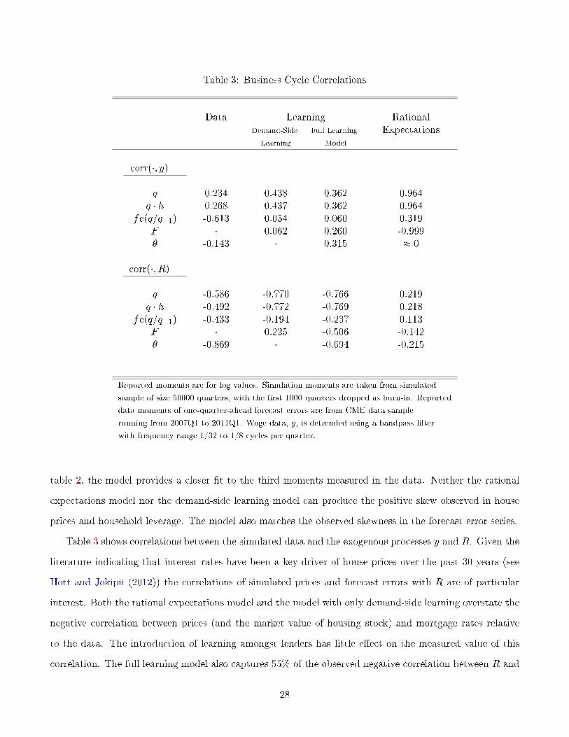
Table 3: Business Cycle Correlations
Data Learning RationalDemand-Side Full Learning Expectations
Learning Model
corr(�; y)
q 0.234 0.438 0.362 0.964q � h 0.268 0.437 0.362 0.964
fe(q=q�1) -0.613 0.054 0.060 0.319F � 0.062 0.260 -0.999� -0.143 � 0.315 � 0
corr(�; R)
q -0.586 -0.770 -0.766 0.219q � h -0.492 -0.772 -0.769 0.218
fe(q=q�1) -0.433 -0.194 -0.237 0.113F � 0.225 -0.506 -0.142� -0.869 � -0.694 -0.215
Reported moments are for log values. Simulation moments are taken from simulated
sample of size 50000 quarters, with the �rst 1000 quarters dropped as burn-in. Reported
data moments of one-quarter-ahead forecast errors are from CME data sample
running from 2007Q1 to 2011Q1. Wage data, y, is detrended using a bandpass �lter
with frequency range 1/32 to 1/8 cycles per quarter.
table 2, the model provides a closer �t to the third moments measured in the data. Neither the rational
expectations model nor the demand-side learning model can produce the positive skew observed in house
prices and household leverage. The model also matches the observed skewness in the forecast error series.
Table 3 shows correlations between the simulated data and the exogenous processes y and R. Given the
literature indicating that interest rates have been a key driver of house prices over the past 30 years (see
Hott and Jokipii (2012)) the correlations of simulated prices and forecast errors with R are of particular
interest. Both the rational expectations model and the model with only demand-side learning overstate the
negative correlation between prices (and the market value of housing stock) and mortgage rates relative
to the data. The introduction of learning amongst lenders has little e�ect on the measured value of this
correlation. The full learning model also captures 55% of the observed negative correlation between R and
28

Figure 6: Standard Deviation of q and fe(q=q�1) Relative to y
0.005 0.01 0.015 0.02 0.025 0.03 0.0351.5
2
2.5
3
Gain
rel.
std
(pri
ce
)
0.005 0.01 0.015 0.02 0.025 0.03 0.0350.4
0.6
0.8
1
rel.
std
(FE
)
rel. std(price)
rel. std(FE)
forecast errors, an improvement upon the demand-side learning model, and comes close to matching the
observed correlation between � and R. As can also be seen in table 3, the full model can also capture the
observed correlation between house prices (and the market value of housing stock) and wages.
Turning to the time-series properties of the model, �gure 7 plots the periodogram of prices for the
three models listed in tables 2 and 3. Under rational expectations house prices fail to display the level of
low-frequency variation seen in the data. This problem is alleviated through the introduction of bounded
rationality in the model. Both the full model as well as the model with only demand-side learning can
capture the bulk of the low frequency (ie. less than 0.2 cycles per quarter) variation in the data, however
the full learning model provides a marginally better �t to the data spectrum. Autocorrelations for forecast
errors and � are shown in table 4. The full learning model matches the �rst order autocorrelation in forecast
errors, however it overstates persistence in the series at higher lags. The learning model also overstates
persistence in household leverage, however it signi�cantly outperforms the rational expectations model in
this regard.
In sum, the model developed here weakly dominates the demand-side learning model along the dimen-
sions discussed. The model captures almost all of the volatility in house prices over the business cycle whilst
providing a closer �t to observed correlations with market fundamentals.
29

Table 4: Autocorrelation
Data� Learning RationalDemand-Side Full Learning Expectations
Learning Model
t (fe(q=q�1)
1 0.412 0.154 0.438 �4:27� 10�4
2 -0.091 -0.037 0.156 �7:19� 10�4
5 -0.068 -0.042 -0.054 �5:10� 10�3
10 -0.282 -0.034 -0.081 �1:08� 10�2
t (�)
1 0.992 � 0.998 0.9992 0.984 � 0.995 0.9995 0.959 � 0.985 0.99810 0.862 � 0.971 0.998
� autocorrelations for � are taken on sample from 1978Q1-2014Q1
Reported moments are for log values. Simulation moments are taken from simulated sample
of size 50000 quarters, with the �rst 1000 quarters dropped as burn-in. Reported data
moments of one-quarter-ahead forecast errors are from CME data sample running from
2007Q1 to 2011Q1. Wage data, y, is detrended using a bandpass �lter with frequency
range 1/32 to 1/8 cycles per quarter.
7 Conclusion
This paper provides a framework for explaining asset price booms. A general equilibrium model with
learning can quantitatively explain US house price growth in the 2000s and account for volatilities in
house prices and forecast errors when agents learn subjective beliefs about prices. The model departs from
established frameworks in allowing for bounded rationality amongst both households and the suppliers of
credit. In demand-side learning models there exists a trade-o� between generating subjective beliefs that
are persistent and at the same time highly responsive to innovations. The interaction between the demand
and credit supply sides of the market under learning boost the persistence in beliefs, thereby breaking this
trade-o�. A single permanent and unanticipated decrease in mortgage rates, consistent with the observed
drop in US interest rates in the early 2000s, produces 20 quarters of price growth whilst capturing the
30

Figure 7: Periodogram of Log House Prices
0 0.05 0.1 0.15 0.2 0.25 0.3 0.35 0.4 0.45 0.5−55
−50
−45
−40
−35
−30
−25
−20
−15
−10
Frequency
Po
wer/
Fre
qu
en
cy
Full Model
Demand−side Learning
REE
Data
total growth in prices observed across the US. The model also outperforms both demand-side learning and
rational expectations models in capturing key business cycle moments.
There are several further issues that can explored using the framework developed here. In particular, the
paper has assumed homogeneous beliefs between households and credit suppliers, however this can be easily
relaxed. The open economy assumption implies that interest rate movements in the model are exogenous.
The model can be augmented to consider endogenous mortgage rates and the in�uence of movements in
mortgage rate expectations amongst households. Similarly, a natural line of inquiry would be to augment
the funding side of the lenders problem and consider the e�ects of uncertainty about �nancial risk.
31

References
Adam, Klaus, Johannes Beutel, and Albert Marcet. 2014. �Stock Price Booms and Expected CapitalGains.� Working Papers 14-12, University of Mannheim, Department of Economics.
Adam, Klaus, Pei Kuang, and Albert Marcet. 2011. �House Price Booms and the Current Account.� NBERMacroeconomics Annual 26:77�122.
Adam, Klaus and Albert Marcet. 2010. �Booms and Busts in Asset Prices.� IMES Discussion Paper Series10-E-02, Institute for Monetary and Economic Studies, Bank of Japan.
���. 2011. �Internal Rationality, Imperfect Market Knowledge and Asset Prices.� Journal of Economic
Theory 146:1224�1252.
Adam, Klaus, Albert Marcet, and Juan Pablo Nicolini. 2013. �Stock Market Volatiliy and Learning.�Working Paper, Federal Reserve Bank of Minneapolis.
Ahearne, Alan G. et al. 2005. �Monetary Policy and House Prices: A Cross-Country Study.� Board ofGovernors of the Federal Reserve System, International Finance Discussion papers, Number 841.
Boz, Ermine and Enrique G. Mendoza. 2014. �Financial innovation. the discovery of risk, and the US creditcrises.� Journal of Monetary Economics 62:1�22.
Branch, William A. 2014. �Imperfect Knowledge, Liquidity and Bubbles.� Working Paper, University ofCalifornia, Irvine.
Branch, William A. and Bruce McGough. 2011. �Bsiness Cycle Theory and Ampli�cation with Heteroge-neous Expectations.� Economy Theory 47:395�421.
Branch, William A., Nicolas Petrosky-Nadeau, and Guillaume Rocheteau. 2014. �Financial Frictions, Hous-ing Market, and Unemployment.� Working Paper, University of California, Irvine.
Bulusu, Narayan, Je�erson Duarte, and Carles Vergaga-Alert. 2013. �Booms and Busts in Houst PricesExplained by Constraints in Housing Suppl.� Working Paper 2013-18, Bank of Canada.
Burnside, Craig, Martin Eichenbaum, and Sergio Rebelo. 2011. �Understanding Booms and Busts inHousing Markets.� Working Paper 16734, National Bureau of Economic Research.
Carceles-Poveda, Eva and Chryssi Giannitsarou. 2008. �Asset Pricing with Adaptive Learning.� Review of
Economic Dynamics 11:629�651.
Case, Karl E. and Robert J. Shiller. 2003. �Is there a Bubble in the Housing Market.� Brookings Papers
on Economic Activity 34:299�362.
Cellarier, Laurent. 2006. �Constant Gain Learning and Business Cycles.� Journal of Macroeconomics
28:51�85.
���. 2008. �Least Squares Learning and Business Cycles.� Journal of Economic Behavior & Organization
68:553�564.
Cheng, Ing-Haw, Sahil Raina, and Wei Xiong. 2012. �Wall Street and the Housing Bubble.� Working Paper,Ross School of Business, University of Michigan.
32

Cho, In-Koo, Noah Williams, and Thomas J. Sargent. 2002. �Escaping Nash In�ation.� Review of Economic
Studies 69:1�40.
Christiano, Lawrence J. and Jonas D.M. Fisher. 2000. �Algorithms for solving dynamic models withoccasionally binding constraints.� Journal of Economic Dynamics and Control 24:1179�1232.
Chu, Yongqiang. 2014. �Credit Constraints, Inelastic Supply, and the Housing Boom.� Review of Economic
Dynamics 17:52�69.
Davis, Morris and Jonathan Heathcote. 2007. �The Price and Quantity of Residential Land in the UnitedStates.� Journal of Monetary Economics 54 (8):2595�2620.
Eusepi, Stefano and Bruce Preston. 2011. �Expectations, Learning and Business Cycle Fluctuations.�American Economic Review 101:2844�2872.
Evans, George W. and Seppo Honkapohja. 2001. Learning and Expectations in Macroeconomics. Princeton:Princeton University Press.
���. 2003. �Expectations and the Stability Problem for Optimal Monetary Policies.� Review of Economic
Studies 70:807�823.
Favilukis, Jack, Sydney C. Ludvigson, and Stijn Van Nieuwerburgh. 2010. �The Macroeconomic E�ects ofHousing Wealth, Housing Finance, and Limited Risk-Sharing in General Equilibrium.� Worker Paper15988, National Bureau of Economic Research.
Gelain, Paolo and Kevin J. Lansing. 2013. �House Prices, Expectations, and Time-Varying Fundamentals.�Working Paper 2013-03, Federal Reserve Bank of San Francisco.
Glaeser, Edward L., Joseph Gyourko, and Albert Saiz. 2008. �Housing Supply and Housing Bubbles.�Journal of Urban Economics 64:198�217.
Granziera, Eleonora and Sharon Kozicki. 2012. �House Price Dynamics: Fundamentals and Expectations.�Working Paper 2012-12, Bank of Canada.
Hott, Christian and Terhi Jokipii. 2012. �Housing Bubbles and Interest Rates.� Swiss National Bank,Working Paper.
Huang, Kevin X.D., Zheng Liu, and Tao Zha. 2009. �Learning, Adaptive Expectations and TechnologyShocks.� The Economic Journal :377�405.
Iacoviello, Matteo. 2011. �Housing Wealth and Consumption.� Board of Governors of the Federal ReserveSystem, International Finance Discussion papers, Number 1027.
Justiniano, Alejandro, Giorgio Primiceri, and Andrea Tambalotti. 2015. �Household Leverage and Delever-aging.� Review of Economic Dynamics 18 (1):3�20.
Kiyotaki, Nobuhiro, Alexander Michaelides, and Kalin NIkolov. 2011. �Winners and Losers in HousingMarkets.� Journal of Money, Credit and Banking 43:255�296.
Kiyotaki, Nobuhiro and John More. 1997. �Credit Cycles.� The Journal of Political Economy 105 (2):211�248.
Kreps, David M. 1998. �Anticipated Utility and Dynamic Choice.� In Frontiers of Research in Economic
Theory, edited by Donald P. Jacobs, Ehud Kalai, Morton I. Kamien, and Nancy L. Shwartz. CambridgeUniversity Press, 242�274.
33

Kuang, Pei. 2014. �A Model of Housing and Credit Cycles.� European Economic Review :419�437.
Luzzetti, Matthew and Seth Neumuller. 2015. �Learning and the Dynamics of Consumer Unsercurted Debtand Bankruptcies.� Working Paper, Wellesley College.
Marshall, Emily and Paul Shea. 2013. �Housing and Endogenous Default.� Working Paper, University ofKentucky.
McCallum, Bennett T. 2007. �E-stability Vis-a-Vis Determinat Results for a Broad Class of Linear RationalExpectations Models.� Journal of Economic Dynamics and Control 31:1376�1391.
Milani, Fabio. 2007. �Expectations, Learning and Macroeconomic Persistence.� Journal of Monetary
Economics 54:2065�2082.
Nakajima, Makoto. 2011. �Understanding House-Price Dynamics.� Business Review Federal Reserve Bankof Philadelphia.
Pancrazi, Roberto and Mario Pietrunti. 2014. �Natural Expectations and Home Equity Extraction.� Work-ing Paper, University of Warwick.
Pastor, Lubos and Pietro Veronesi. 2006. �Was There a NASDAQ Bubble in the Late 1990s?� Journal of
Financial Economics 81:61�100.
Piazzesi, Monika and Martin Schneider. 2009. �Momentum Traders in the Housing Market: Survey Evidenceand a Search Model.� Worker Paper 14669, National Bureau of Economic Research.
Preston, Bruce. 2005. �Learning about Monetary Policy Rules when Long-Horizon Expectations Matter.�International Journal of Central Banking 1:81�126.
Saiz, Albert. 2010. �The Geographic Determinants of Housing Supply.� The Quarterly Journal of Economics125:1253�1296.
Sargent, Thomas J. 1999. The Conquest of American In�ation. Princeon University Press.
Sinha, Arunima. 2011. �Learning and the Yield Curve.� Working Paper, Santa Clara University, LeavySchool of Business.
Wheaton, Williams C. and Gleb Nechayev. 2010. �Residential Investment: a Sleeping Giant.� Unpublished,MIT Center for Real Estate.
Williams, Noah. 2003. �Adaptive learning and business cycles.� Unpublished, Princeton University.
���. 2012. �Financial Instability via Adaptive Learning.� Working Paper, University of Wisconsin -Madison, Department of Economics.
Winkler, Fabian. 2015. �The Role of Learning for Asset Prices, Business Cycles and Monetary Policy.�Working Paper, Board of Governors of the Federal Reserve.
Zhang, Cathy. 2012. �Bad News for News Shocks?� Working Paper, University of California, Irvine.
34

A Additional Figures
Figure A.1: Maximum Log Price Deviation and Length of Propagation Following R Drop
0.01
0.011
0.012
0.013
0.014
0.015
0.016
gain
0.050.055
0.060.065
0.070.075
depreciation rate
0.1
0.15
0.2
0.25
0.3
0.35
0.4
0.45
maxim
um
lo
g d
evia
tio
n
(a) Maximum Log Price Deviation
0.010.011
0.0120.013
0.0140.015
0.016
gain
0.050.055
0.060.065
0.070.075
depreciation rate
6
8
10
12
14
16
18
len
gth
of
pro
pag
ati
on
(b) Length of Propagation Following R Drop
35

B Aggregation of Household Problem to Representative Agent
This appendix outlines the aggregation of the household problem in section 3.1 to a representative agent.
Assume that all notation is in terms of individual household i in a heterogeneous agents economy. All
agents are assumed to have the same information, preferences, credit constraint, etc... Assume that the
households have access to a complete set of Arrow-Debreu securities in consumption goods. Also assume
that the household has access to a security that is indexed to house prices (in other words, a security
that delivers in units of housing). Assume that for both of these securities the household is exempt from
obligations/payments if it defaults. For ease of notation, physical capital kt is omitted from the exposition,
but its presence does not alter the steps outlined below.
� The budget constraint and credit constraint of of household i are
cit + qthit +Rbit�1 + pcte
ict + pht e
iht = yit + (1� �)hit�1 + bit + eict�1 + qte
iht�1 (31)
bit �
��
R
�~Et[qt+1]h
it � ~Qth
it (32)
these imply
cit + (qt � ~Qt)hit = ~yit +
n(1� �)qt �R ~Qt�1
ohit�1 (33)
where
~yit = yit � pcteict � pht e
iht + qte
iht�1 + eict�1 (34)
� Let
1� �t = Pr
�qtqt�1
< �it�
1� �
�= Pr
�Defaultj
qtqt�1
�(35)
� If the household defaults, it loses its stock of housing and no longer has to repay its debt bt�1
� The household's maximization problem can be written as follows
maxEPt
8>>>><>>>>:Xt
�t
0BBBB@
u(cit; hit) + �it
yit + (1� �)qt�th
it�1 + bit + �te
ict�1 + qt�te
iht�1:::
�cit � qthit �R�tb
it�1 � pcte
ict � pht e
iht
!
+�it��EPt fqt+1gh
it �Rbit
�
1CCCCA
9>>>>=>>>>;
(36)
� The �rst order conditions for this problem are
pct = � � EPt
��it+1�it
�t+1
�(37)
pht = � � EPt
��it+1�it
�t+1qt+1
�(38)
�it = uc(cit; h
it) � uic(t) (39)
�it =�itR� ��it+1�t+1 (40)
qt�it = uih(t) + �it�qt+1 + �(1� �)�it+1qt+1�t+1 (41)
36

=) qt =uih(t)
uic(t)+ E
Pt
���(1� �) �
�it+1�it
� �t+1 +�
R
�� qt+1 � ��
�EPt qt+1
� �it+1�it
�t+1
�(42)
� From the securities market:
pct = � � EPt
��it+1�it
�t+1
�= � � EPt
"�jt+1
�jt�t+1
#(43)
pht = � � EPt
��it+1�it
�t+1qt+1
�= � � EPt
"�jt+1
�jt�t+1qt+1
#(44)
� So these markets imply that the price of consumption and default-weighted housing is the same
for all agents
� Rewrite the budget constraint, and combine with the assumption that the borrowing constraint binds
cit + qthit +R ~Qt�1h
it�1 = ~yit + (1� �)qth
it�1 + ~Qth
it (45)
=) cit + (qt � ~Qt)hit = ~yit +
�(1� �)qt �R ~Qt�1
�hit�1 (46)
� From the household Euler
qt =1� c c
�cithit
+ �(1� �) EPt
��it+1�it
�t+1qt+1
�| {z }
common across agents
����EPt qt+1
�EPt
��it+1�it
�t+1
�| {z }
comon across agents
:::
+�
REPt [qt+1]| {z }~Qt
=)cithit
=1� c c
�qt � ~Qt � �(1� �)EPt
��it+1�it
�t+1qt+1
�+ ��
�EPt qt+1
�EPt
��it+1�it
�t+1
��| {z }
�Bt, common across agents
=) cit = Bthit (47)
� Substitute this into the modi�ed budget constraint (46)
cit + (qt � ~Qt)hit = ~yit +
�(1� �)qt �R ~Qt�1
�hit�1
=) cit + (qt � ~Qt)B�1t cit = ~yit +
�(1� �)qt �R ~Qt�1
�hit�1
=)�1 + (qt � ~Qt)B
�1t
�cit = ~yit +
�(1� �)qt �R ~Qt�1
�hit�1
=)�1 + (qt � ~Qt)B
�1t
�Xi
cit =Xi
~yit +�(1� �)qt �R ~Qt�1
�Xi
hit�1 (48)
37

� Note that
Xi
cit = CtXi
hit = Ht
Xi
~yit =Xi
�yit � pcte
ict � pht e
iht + qte
iht�1 + eict�1
�= Yt � pct
Xi
eict| {z }=0
�phtXi
eiht| {z }=0
+qtXi
eiht�1| {z }=0
+Xi
eict�1| {z }=0
where the zeros are the result of market clearing in securities
=)�1 + (qt � ~Qt)B
�1t
�Ct = Yt +
�(1� �)qt �R ~Qt�1
�Ht�1 (49)
which is equivalent to a representative agents' choice
38

C Solving the Household Problem
The solution to the household problem is computed using a parameterized expectations algorithm (PEA).
Rewriting the household Euler (17) in simpli�ed notation
qt �uh(t)
uc(t)= E
Pt [(qt+1; ct+1; ht+1)jct; ht; bt; qt;mt; �t; yt; Rt] (50)
The expectation on the right hand side is approximated as
exp (e(Xt; )) (51)
The basis functions for e(�) are the Chebyshev polynomials. The vector of state variables for the household,
Xt, is (ht�1; kt�1; qt;mt; �t; yt; Rt)35. De�ne to be a coe�cient vector. The order of the approximation
along each dimension is given by (rh; rk; rq; rm; r�; ry; r�), hence is an rh�rk�rq�rm�r��ry�r� vector.
Let i(x) denote the Chebyshev polynomial of order i evaluated at x. Because the Chebyshev polynomials
are de�ned on [�1; 1] the state variables are rescaled according to
~x = 2x� �x
�x� x� 1 2 [�1; 1]
The approximating function e(Xt; ) can be written
e ((h; k; q;m; �; y; R); ) = T (h; k; q;m; �; y; R) (52)
= (Th(h) Tk(k) Tq(q) Tm(m) T�(�) Ty(y) TR(R))
where Tx(x) = ( 0(~x); 1(~x); :::; rx(~x))
The coe�cient vector is solved by appealing to the Chebyshev interpolation theorem and setting the
approximating function e(�) to be exact at the Chebyshev nodes. therefore solves the system
exp�EPt [(�)]
�� e ((h; k; q;m; �; y; R); ) = 0 8 vectors of nodes (h; k; q;m; �; y; R) (53)
which is an rh � rk � rq � rm � r� � ry � r� system of equations with rh � rk � rq � rm � r� � ry � r�
unknowns. (53) is solved by an iterative procedure. Let x denote the rx-vector of Chebyshev nodes along
dimension x and X = h� k � q � m� � � y � R
1. Start from an initial guess 0
2. Compute the vector e (�; 0) for all Chebyshev nodes h� k � q � m� � � y � R using (52)
e�h� k � q � m� � � y � R; 0
�= T (h; k; q; m; �; y; R) � 0
� B � 0
3. Given e(X; 0) one can back out a corresponding vector of choice variables (ct; ht; bt; kt) from the
35In order to limit the size of the space the following approximation is applied bt ��tRt
qtmtht.
39

model equations outlined in section 3.1, call this �(X; 0). Compute the expectation EPt [(�)] at all
the Chebyshev nodes using a Gaussian quadrature, call this vector Y (X; 0);
Y (X; 0) =
��qt+1; ct+1
��(X; 0)
�; ht+1
��(X; 0)
�jX; �(X; 0)
�dF (yt+1; qt+1jqt; yt;P)
4. Compute
� =�B0B
��1B0 log Y (X; 0)
5. Update the guess
1 = ! � + (1� !) 0
for ! 2 (0; 1)36
6. Repeat 1-5 until convergence37
36The procedure fails to converge when 1 = �, necessitating this step.37Further details on such methods can be found in Christiano and Fisher (2000).
40

D Data Appendix
US. Bureau of Economic Analysis, Compensation of employees: Wages and salaries [A576RC1Q027SBEA],retrieved from FRED, Federal Reserve Bank of St. Louis,https://research.stlouisfed.org/fred2/series/A576RC1Q027SBEA/
US. Bureau of Labor Statistics, Consumer Price Index for All Urban Consumers: All Items Less Food &Energy [CPILFENS], retrieved from FRED, Federal Reserve Bank of St. Louis,https://research.stlouisfed.org/fred2/series/CPILFENS/, August 1, 2015.
US. Bureau of Economic Analysis, Personal Consumption Expenditures [PCECA], retrieved from FRED,Federal Reserve Bank of St. Louis,https://research.stlouisfed.org/fred2/series/PCECA/, August 1, 2015.
US. Bureau of Economic Analysis, Personal consumption expenditures: Services: Housing: Imputed rentalof owner-occupied nonfarm housing [DOWNRC1A027NBEA], retrieved from FRED, Federal ReserveBank of St. Louis,https://research.stlouisfed.org/fred2/series/DOWNRC1A027NBEA/, August 1, 2015.
US. Bureau of Economic Analysis, Shares of gross domestic product: Personal consumption expenditures:Durable goods [DDURRE1A156NBEA], retrieved from FRED, Federal Reserve Bank of St. Louis,https://research.stlouisfed.org/fred2/series/DDURRE1A156NBEA/, August 1, 2015.
US. Bureau of Economic Analysis, Shares of gross domestic product: Personal consumption expenditures:Nondurable goods [DNDGRE1A156NBEA], retrieved from FRED, Federal Reserve Bank of St. Louis,https://research.stlouisfed.org/fred2/series/DNDGRE1A156NBEA/, August 1, 2015.
US. Bureau of Economic Analysis, Shares of gross domestic product: Personal consumption expenditures:Services [DSERRE1A156NBEA], retrieved from FRED, Federal Reserve Bank of St. Louis,https://research.stlouisfed.org/fred2/series/DSERRE1A156NBEA/, August 1, 2015.
Freddie Mac, 30-Year Fixed Rate Mortgage Average in the United States [MORTGAGE30US], retrievedfrom FRED, Federal Reserve Bank of St. Louis,https://research.stlouisfed.org/fred2/series/MORTGAGE30US/, August 1, 2015
US. Federal Housing Finance Agency, All-Transactions House Price Index for the United States [USSTHPI],retrieved from FRED, Federal Reserve Bank of St. Louis,https://research.stlouisfed.org/fred2/series/USSTHPI/, August 1, 2015.
Board of Governors of the Federal Reserve System (US), Households and Nonpro�t Organizations; CreditMarket Instruments; Asset, Level [HSTCMAHDNS], retrieved from FRED, Federal Reserve Bank ofSt. Louis,https://research.stlouisfed.org/fred2/series/HSTCMAHDNS/, August 1, 2015.
Board of Governors of the Federal Reserve System (US), Households and Nonpro�t Organizations; CreditMarket Instruments; Liability, Level [CMDEBT], retrieved from FRED, Federal Reserve Bank of St.
41

Louis,https://research.stlouisfed.org/fred2/series/CMDEBT/, August 1, 2015.
Board of Governors of the Federal Reserve System (US), Real Gross Domestic Product [GDPC1], retrievedfrom FRED, Federal Reserve Bank of St. Louis,https://research.stlouisfed.org/fred2/series/GDPC1/, August 1, 2015.
Board of Governors of the Federal Reserve System (US), Households and Nonpro�t Organizations; totalmortgages; asset, Level [HNOTMAQ027S], retrieved from FRED, Federal Reserve Bank of St. Louis,https://research.stlouisfed.org/fred2/series/HNOTMAQ027S/, August 1, 2015.
Board of Governors of the Federal Reserve System (US), Households and Nonpro�t Organizations; totalmortgages; liability [HNOTMLQ027S], retrieved from FRED, Federal Reserve Bank of St. Louis,https://research.stlouisfed.org/fred2/series/HNOTMLQ027S/, August 1, 2015.
Board of Governors of the Federal Reserve System (US), Households and Nonpro�t Organizations; CreditMarket Instrutments; Asset, Level [CMIABSHNO], retrieved from FRED, Federal Reserve Bank of St.Louis,https://research.stlouisfed.org/fred2/series/CMIABSHNO/, August 1, 2015.
Board of Governors of the Federal Reserve System (US), Households and Nonpro�t Organizations; HomeMortgages; Liability [HMLBSHNO], retrieved from FRED, Federal Reserve Bank of St. Louis,https://research.stlouisfed.org/fred2/series/HMLBSHNO/, August 1, 2015.
Board of Governors of the Federal Reserve System (US), Households; Owner's Equity in Real Estate asa Percentage of Household Real Estate, Level [HOEREPHRE], retrieved from FRED, Federal ReserveBank of St. Louis,https://research.stlouisfed.org/fred2/series/HOEREPHRE/, August 1, 2015.
Board of Governors of the Federal Reserve System (US), Households and Nonpro�t Organizations; CreditMarket Instruments; Liability, level [HSTCMDODNS], retrieved from FRED, Federal Reserve Bank ofSt. Louis,https://research.stlouisfed.org/fred2/series/HSTCMDODNS/, August 1, 2015.
Board of Governors of the Federal Reserve System (US), Households; Owner's Equity in Real Estate, Level[OEHRENWBSHNO], retrieved from FRED, Federal Reserve Bank of St. Louis,https://research.stlouisfed.org/fred2/series/OEHRENWBSHNO/, August 1, 2015.
Board of Governors of the Federal Reserve System (US), Delinquency Rate On Single-Family ResidentialMortgages, Booked In Domestic O�ces, All Commercial Banks [DRSFRMACBS], retrieved from FRED,Federal Reserve Bank of St. Louis,https://research.stlouisfed.org/fred2/series/DRSFRMACBS/, August 1, 2015.
S&P Dow Jones Indices LLC, S&P/Case-Shiller 10-City Composite Home Price Index [SPCS10RNSA],retrieved from FRED, Federal Reserve Bank of St. Louis,https://research.stlouisfed.org/fred2/series/SPCS10RNSA/, August 1, 2015.
42

Davis, Morris A. and Jonathan Heathcote, 2007, "The Price and Quantity of Residential Land in the UnitedStates," Journal of Monetary Economics, vol. 54 (8), p. 2595-2620; data located at Land and PropertyValues in the U.S., Lincoln Institute of Land Policy http://www.lincolninst.edu/resources/
Saiz, Albert. 2010. "The Geographic Determinants of Housing Supply," The Quarterly Journal of Eco-nomics 125: 1253-1296.
U.S. Dept. of Commerce, Bureau of the Census. AMERICAN HOUSING SURVEY, 2005: NATIONALMICRODATA. ICPSR04593-v1. Washington, DC: U.S. Dept. of Commerce, Bureau of the Census[producer], 2006. Ann Arbor, MI: Inter-university Consortium for Political and Social Research [dis-tributor], 2007-06-13. http://doi.org/10.3886/ICPSR04593.v1
Bloomberg L.P. CME Case Shiller Home Price Futures 1/5/2007 to 1/2/2015. Retrieved May 20, 2015from Bloomberg database.
43