Can Gambling Increase Savings?

Empirical Evidence on Prize-linked Savings Accounts

Shawn Cole

Harvard Business School and NBER

Benjamin Iverson

Northwestern University

Peter Tufano

University of Oxford - Saïd Business School and NBER

February 2016

Keywords: Household finance; Banking; Savings; Prize-linked savings; Lottery

JEL classification: D14; E21; G21; L83;

__________________________________________________________________ The authors can be contacted via the following email addresses: Shawn Cole: scole@hbs.edu; Ben Iverson: b-

iverson@kellogg.northwestern.edu; Peter Tufano: peter.tufano@sbs.ox.ac.uk.

We are grateful to Daryl Collins, Brian Melzer, Dan Schneider and seminar participants at the Boulder Summer

Conference on Consumer Financial Decision Making, Brigham Young University, NBER Household Finance

Conference, Northwestern University, Research in Behavioural Finance Conference at Erasmus University, the

University of Illinois – Chicago, and the University of Oxford for helpful comments. Veronica Postal, William

Talbott and Xiwen Wang provided excellent research assistance. We are also grateful to First National Bank (FNB),

and especially Francois Thiart and Robert Keip, for assistance with this project and valuable feedback. None of the

authors has ever received compensation from FNB or any of its subsidiaries; all authors declare they have no

material interest in FNB. We acknowledge financial support from HBS' Division of Research and Faculty

Development and the University of Oxford, Saïd Business School.

Can Gambling Increase Savings?

Empirical Evidence on Prize-linked Savings Accounts

Abstract

This paper studies the adoption and impact of prize-linked savings (PLS) accounts, which offer random,

lottery-like payouts to individual account holders in lieu of interest. Using micro-level data from a bank

offering these products in South Africa, we show that PLS is attractive to a broad group of individuals,

across all age, race, and income levels. Financially-constrained individuals and those with no other

deposit accounts are particularly likely to open a PLS account. Participants in the PLS program increase

their total savings on average by 1% of annual income, a 38% increase from the mean level of savings.

Deposits in PLS do not appear to cannibalize same-bank savings in standard savings products. Instead,

PLS appears to serve as a substitute for lottery gambling. Exploiting the random assignment of prizes, we

also present evidence that prize winners increase their investment in PLS, sometimes by more than the

amount of the prize won, and that large prizes generate a local “buzz” which lead to an 11.6% increase in

demand for PLS at a winning branch.

2

I. Introduction

Personal savings often serve as the first available buffer for households when faced with job loss,

healthcare costs, or other financial shocks. However, recent evidence suggests that a large percentage of

households maintain little to no savings, despite potentially high returns to saving (Dupas and Robinson

2013) and significant costs of financial fragility (Lusardi, Schneider, and Tufano 2011; FDIC 2012). In

light of this, economists and policymakers have considered financial innovations to encourage savings,

such as default options, commitment devices, or savings reminders.1 This paper examines prize-linked

savings (PLS) products, which provide participants the chance to win prizes by saving money. The

promise of PLS is that it can deliver the utility of lottery play while simultaneously encouraging

individuals to substitute toward higher financial security.

While PLS programs have existed for hundreds of years and are prevalent around the world,

including their recent legalization in the U.S., 2

they have received little academic attention. Studies to

this point have focused on either high-level, macro data (Tufano 2008), small-scale surveys (Tufano,

Maynard, and De Neve 2008), or laboratory experiments (Atalay et al. 2014; Filiz-Ozbay et al. 2015).3 In

this paper, we use account-level data from a PLS program run by one of the largest banks in South Africa

to demonstrate that PLS is particularly attractive to individuals with no traditional savings accounts and

those with high debt levels. Importantly, we show that PLS participants tend to significantly increase

overall savings rates and that at least some of this increase in net savings comes from reduced lottery

play.

PLS accounts differ from standard savings accounts in that they offer individual savers a

stochastic, heavily-skewed return as opposed to a predetermined interest rate. Depositors in a PLS

account are entered periodically into a drawing in which their chance at winning a potentially large prize

1 See, for example, Carroll et al. (2009), Thaler and Benartzi (2004), Ashraf, Karlan, and Yin (2006) and Karlan et

al. (2012). Tufano and Schneider (2008) provide an overview of policy proposals. 2 In December 2014, the American Savings Promotion Act legalized no-risk cash-prize savings raffles, making PLS

legal in the U.S. for the first time. 3 One exception is Cookson (2014), who uses micro-level data from casinos to examine the impact of PLS on

gambling expenditures.

3

(or smaller prizes) is a function of the amount they have deposited. In aggregate, all savers receive a total

amount of prizes (interest payments) that may approximate market rates, but this lottery-like system

changes the payoff structure for saving, adding an element of risk and, possibly, excitement to holding

money in the account.

Given the widespread demand for lottery gambling, it has been hypothesized that the lottery-like

incentive structure of PLS could be attractive to large numbers of participants (Kearney et al. 2010).

Indeed, participation rates in the UK’s Premium Bond program, a PLS product, are estimated to be

between 22 and 40 percent of UK citizens (Tufano 2008). The PLS account examined in this paper—the

“Million-a-Month Account,” or MaMa, offered by First National Bank (FNB), a large South African

retail bank—saw similarly robust demand: within 18 months of the start date of the program there were

more PLS accounts than regular savings accounts at the bank, and within 3 years PLS deposits amounted

to R1.4 billion at the bank, as compared to total savings of R4.5 billion in the comparable standard

savings account (Figure 1).

[FIGURE 1]

A more vital question, however, is whether PLS can increase savings for individuals who avoid

traditional saving products. In particular, the 2013 Survey of Consumer Finances shows that only 31.7%

of households in the lowest income quintile regularly save. At the same time, low-income households

account for a disproportionate share of lottery expenditures in the U.S., with lottery expenditures totaling

over 5% of income for those in the lowest income brackets (Clotfelter et al. 1999). Further, Lusardi et al.

(2011) show that gamblers are particularly prone to lack precautionary savings. This suggests that PLS

may be uniquely positioned to attract savings from individuals who are less likely to maintain emergency

savings in the formal banking sector. Using account-level data on employees of FNB, we find that

individuals who had no standard savings accounts were 12.2 percentage points more likely to open a PLS

account than those with accounts. In addition, employees who were the largest net borrowers from the

bank were most likely to open a PLS account, while those with moderate savings amounts were least

likely. Corroborating this, we also use survey data from individuals that live near FNB branches and find

4

that usage of PLS was especially strong in areas with low take-up of financial products and where a high

percentage of individuals felt unable to repay their debts.

It is also important to evaluate whether PLS accounts attract new savings or merely cannibalizes

regular savings. We show that bank employees who open a PLS account tend to increase their net

savings at First National Bank by about 1% of their annual income, a 38% increase from the mean level

of savings. We do not find any evidence that employees who open PLS accounts decrease their savings

in standard FNB savings products. Rather, we show that they tend to increase deposits in regular savings

accounts as well, which is surprising as one would expect some substitution effect to be present. Because

the introduction of MaMa was not a randomized trial, we cannot attribute a causal relationship between

PLS usage and savings rates. However, the positive relationship between PLS usage and regular savings

suggests that few individuals removed funds from standard accounts to fund PLS. Further, using the

random size of jackpots in the South Africa National Lottery, we present causal evidence that demand for

the PLS program nationwide was especially strong in periods when the jackpot of the national lottery was

small. Thus, we find that PLS and lottery gambling act as substitutes.4

A unique feature of PLS is the fact that “lucky” account holders win prizes. In the PLS program

run by First National Bank, each month a total of 113 prizes were awarded, including a grand prize of

R1,000,000 (approximately $150,000) and R500,000 in smaller prizes. We track the accounts of these

randomly selected prize-winners and test whether they are more likely to close their accounts after

winning, or whether winning a prize induces them to invest more in PLS. Relative to non-winners,

winners of small R1,000 prizes are 4.2 percentage points more likely to close their accounts within one

year of winning their prize, while winners of larger prizes are no more likely to close their accounts.

Despite being more likely to close their accounts, however, prize winners on average keep substantially

more in their accounts than those who did not win prizes. In some cases, prize winners increase their

4 This is consistent with evidence in Atalay et al. (2014) and Filiz-ozbay et al. (2015), which use experiments to

show that PLS demand is especially strong among lottery players, and Cookson (2014) who shows that casino

gambling decreases when PLS products are introduced in the U.S.

5

account balances in PLS by more than the amount won, indicating that this increased investment in PLS is

more than just a wealth effect. This increased savings is persistent for at least one year after winning.

We also find that large prize winners create a “buzz” that generates more demand for PLS in the

local area. In particular, bank branches which had a R1,000,000 prize winner experienced 11.6% excess

growth in PLS deposits (over and above the amount awarded as a prize) in the month after the win,

relative to all other bank branches.5 Thus, the excitement of winning a prize has spillover effects that also

serve to increase savings by other individuals.

Overall, our findings demonstrate that creating a lottery-like reward structure for savings products

can generate new savers and new saving, in particular by financially fragile individuals with high debt

levels and who do not use traditional savings accounts. Importantly, we show that these results hold in a

large sample of individuals in the field and that the effects are economically large and long-lasting. While

it appears that PLS can provide a natural way for low-wealth individuals to increase savings, PLS is not a

panacea. Although we show that this increased saving is funded at least partially from reduced lottery

expenditure, it is also possible that individuals reduce consumption or investment in other areas in order

to fund their PLS account. Thus, similar to other studies that show increases in household savings, the

welfare implications of PLS are difficult to test.6

The remainder of the paper is organized as follows. Section II gives background information on

First National Bank’s PLS product and the data used in our analysis. Section III provides results on the

characteristics of PLS participants, while Section IV presents evidence on whether PLS reduces deposits

in regular savings products or in the amount of lottery gambling. Section V then discusses how winning a

prize affects both the prize winner and others nearby. Section VI concludes.

II. Background and Data

A. First National Bank’s Prize-Linked Savings Product

5 This finding is similar to Guryan and Kearney (2008), who show that lottery expenditures are higher at “lucky

stores” that sell winning lottery tickets. 6 We discuss welfare further in the conclusion of the paper.

6

The data for this paper come from First National Bank, the retail and commercial bank subsidiary

of FirstRand Bank Limited, the third largest bank in South Africa.7 First National Bank introduced a PLS

account in January, 2005 in an effort to expand its deposit base among low-income and unbanked

individuals (see Cole et al. 2008, who also discuss the informal savings programs that exist in South

Africa).

First National called its PLS account the "Million-a-Month Account," or MaMa, and awarded a

grand prize of R1,000,000 to one random account-holder each month, with the winning account number

announced on national television. In addition to the grand prize, the bank initially also awarded two

prizes of R100,000, 10 prizes of R20,000, and 100 prizes of R1,000 each month. In September, 2007, the

bank doubled the number of smaller prizes given each month, awarding four R100,000 prizes, 20

R20,000 prizes, and 200 R1,000 prizes. Throughout the program, each account-holder received one entry

into the lottery for each R100 held in her account.8 MaMa accounts were 32-day notice accounts,

meaning that if a customer wished to withdraw some of her funds she must notify the bank 32 days in

advance of the withdrawal.9 The most comparable account at First National to MaMa was a standard 32-

day notice account, which paid interest on a variable scale depending on the customer's balance in the

account. As of November, 2004, for balances below R10,000 the 32-day account paid 4% annual interest,

for balances between R10,000 and R25,000 it paid 4.25% APR, and for balances from R25,000 to

R250,000 the APR ranged from 4.5% to 4.75% (Cole et al. 2008).

In contrast to the regular 32-day account, the expected return to holding MaMa balances

depended on the amount of deposits held in the accounts. As the total amount of deposits increased, the

expected return on a 100 Rand deposit decreased, because the chance of winning a prize declined. The

new MaMa accounts proved to be quite popular, and deposits increased dramatically in the first months

7 There were a total of 17 banks functioning in South Africa in 2008, of which the four largest account for 91% of

total assets (South African Reserve Bank 2008). 8 Initially, the accounts paid no interest at all, but the bank began paying a 0.25% interest rate on deposits in addition

to the random prizes in September 2005. There was no discontinuous increase in PLS demand when this change was

made. 9 32-day notice accounts are common in South Africa and are offered by all of the major banks there.

7

(Figure 1). Although the total amount held in MaMa accounts never approached the aggregate balance of

the regular 32-day accounts, the number of MaMa accounts exceeded that of regular 32-day accounts by

June 2006, a mere 18 months after the product was launched. Because of this growth, the expected

interest rate on MaMa accounts declined rapidly. When the first drawing was held in March 2005 (three

months after the start date of the program), the expected annualized interest rate for holding R100 in a

MaMa account was about 12.2%, due to the relatively small amount of total deposits. However, as the

popularity of the program grew, the expected return quickly dropped, and by December 2005 the rate was

3.64%, slightly lower than that offered by the regular 32-day account.10

At its lowest, the expected

interest rate on MaMa accounts was 1.59% in August 2007, just before the number of prizes was

doubled.11

An individual with a preference for lottery-like returns could duplicate the PLS structure by

depositing funds in a regular 32-day account and then using the interest earned from this account to

purchase lottery tickets. This strategy imitates the MaMa account by combining two other readily

available alternatives, and is thus a useful comparison to the MaMa expected return. From 2005-2008,

the expected return on the South African National Lottery was about 46 cents per Rand invested.12

An

individual seeking a skewed return could have deposited, say, R100 (the amount needed for one entry in

the MaMa program) in a regular 32-day account and earned R4 of interest in a given year. If he then used

the R4 to purchase lottery tickets, his expected winnings would amount to about R1.86, giving a net

return of 1.86% on his investment of R100. As noted above, expected returns in the MaMa program were

significantly higher than this amount early on, but dropped to an amount quite close to this as the

popularity of the program grew. In MaMa’s final year, expected returns averaged 1.81% and were quite

10

Barberis and Huang (2008) show that an asset with lottery-like payoffs can earn negative excess returns when

investors overweight small probabilities, as in cumulative prospect theory (Tversky and Kahneman 1992). 11

One would expect that MaMa demand would fall as the PLS expected return decreases relative to the interest rate

in regular 32-day accounts. In unreported regressions, we have tested whether this is the case. We find that the

coefficients are in the expected direction, but that the effect is impossible to separate from a linear time trend, due to

the fact that MaMa usage was quickly growing throughout our sample period. 12

This negative 54% return is similar to that found for other lotteries (e.g. Thaler and Ziemba, 1988).

8

stable, suggesting that equilibrium PLS returns settled near what could have been earned via this synthetic

PLS-like investment.

The MaMa program only lasted until March 2008, when it was deemed a violation of the Lottery

Act of 1997 by the Supreme Court of Appeals (FirstRand Bank v. National Lotteries Board 2008). In

South Africa, as has historically been the case in the U.S., the government holds a monopoly on lotteries.

Although First National argued that its program wasn't technically a lottery, since all principal was

preserved, it failed to convince the courts and was forced to end the program. At the end of March, all

MaMa accounts were converted to regular 32-day accounts, and account holders were allowed to

withdraw their deposits if they chose to do so. The data provided by First National ends in July 2008,

four months after the program ended. During that time period, aggregate MaMa balances fell 16.2% in

April 2008, and an additional 11.8% in May. However, balances held steady in June and July, at which

point our data end. Thus, while some participants in the program did withdraw their funds, over 77% of

all PLS deposits remained in the bank for at least four months after the accounts converted to standard

savings products.

B. Data

Most of the data for this paper come directly from First National Bank, which provided three

main datasets: branch-level data for all bank branches, anonymized account-level data for all bank

employees, and anonymized account-level data for all prize winners. The bank also provided us with

bank-wide data on total accounts and total deposits held in MaMa accounts at a daily frequency. We

augment the data from First National Bank with the 2005 FinScope financial survey of South Africa,

provided by FinMark Trust. Details of each dataset are described below.

B.1. First National Bank Data

First National provided both branch-level and account-level data for this paper. At the branch

level, we have monthly observations for each of 604 bank branches from January 2003 through July 2008.

For each month, we observe the total number of accounts and total Rand balance held at the branch in

9

both standard 32-day accounts and MaMa accounts. Table I provides summary statistics of the total

number of accounts and total deposits at each branch as of March 2008, when the MaMa program ended.

[TABLE I]

In addition to branch-level time series data, we also observe branch-level demographic

characteristics of depositors in both 32-day and MaMa products for one snapshot taken in June 2008, 3

months after the MaMa program ended. This allows us to compare the characteristics of MaMa

participants to those of typical savers, which we do in Table I. With respect to race, MaMa depositors are

less likely to be white, and more likely to be Asian or of mixed race.13

Men account for a total of 52% of

MaMa deposits, as compared to only 46% of regular 32-day deposits, suggesting that the lottery payoff

structure might be more attractive to men than women, perhaps due to lower risk aversion (Eckel and

Grossman 2008) or overconfidence (Barber and Odean 2001). MaMa participants also tend to be younger

than standard 32-day account holders (Figure 2, Panel A). This is important, as younger individuals also

tend to be those who maintain less precautionary savings (Lusardi, Schneider, and Tufano 2011).

[FIGURE 2]

The income profile of MaMa savers appears to be similar to that of regular savers (Figure 2,

Panel B). Specifically, those in the lowest income bracket account for a similar share of total 32-day

balances (45%) as MaMa balances (42%). However, more detailed analysis presented in Section III

shows that those with lower income are somewhat more likely to use PLS. More importantly, evidence in

Section III shows that, after controlling for income, bank employees with lower net savings (or higher

debt) at FNB are more likely to use MaMa. Thus, despite similar income profiles, it is likely that the

wealth levels of PLS users differ from those of regular savings account users.

In addition to the relatively coarse branch-level data, we also analyze account-level data for

employees of First National Bank. This dataset contains month-by-month information on account

balances of 38,256 employees of First National Bank for the time period from January 2005 - March

13

Black persons are those of native African descent. Asian persons include those of Indian descent.

10

2008. For each employee, we observe the month-end balance of their 32-day savings, checking, money

market14

, and MaMa accounts. In addition, we also have a snapshot of the employee's race, gender, age,

income estimate15

, and the region of South Africa in which they work. Summary statistics of employee

account balances are provided in Table I, Panel C.

Of the 38,256 employees, 12,237 had their employment terminated at some point during the

sample period. In all regressions, we include an ex-staff dummy to control for these individuals, but our

results are unchanged if these individuals are removed completely.

There are both advantages and disadvantages to working with staff data. Using account-level

data we get much finer estimates of the effects of PLS. However, as the staff of the bank is not a

representative sample of the South African population, this subsample may limit external validity. For

example, only 41% of bank employees are black as compared to 73% in the population at large. Of more

particular concern is the fact that bank employees are likely better educated and earn more than the

population in general. The average First National employee earns R175,963 per year, while in 2006

average household income in South Africa was estimated to be R74,589 (Statistics South Africa 2008).

Finally, just over 22% of the staff in our sample have no checking, money market, 32-day, or PLS

account at FNB. Nationwide, about 47% of individuals were completely unbanked in South Africa in

2005. To the extent possible, we control for staff characteristics in our analysis, but we do note that there

are large differences between the staff sample and the general population.

Another potential limitation of the staff dataset is that we can only observe deposit accounts held

at FNB, and thus we do not observe their total portfolio if they hold savings elsewhere. However, based

on FinScope Survey data (described below), we estimate that only 3.3% of South Africans have accounts

at multiple banks, conditional on having at least one account. Meanwhile, of survey respondents that

reported having no bank accounts, only 6.3% maintain any savings at home. In addition, one would

14

The money market account was a special account available only to staff of the bank that was launched in July

2007, towards the end of the sample period. 15

Income data was not directly available from First National and was instead estimated by the bank according to an

internal model.

11

expect that the majority of First National employees would do most or all of their banking at First

National due to familiarity with the products, the ease of banking where you work, extra benefits of

banking at work (in particular the ability to utilize overdraft facilities, as discussed below), and likely

encouragement to use the products. Thus, although we cannot observe the entire portfolio of all

employees, we likely have a relatively comprehensive view of staff banking behavior.

An important aspect of the staff data is that it contains information on checking account balances,

which are often negative. Bank staff can easily obtain an overdraft facility on their checking accounts;

this facility offers flexible repayment possibilities. These negative balances can be interpreted as

unsecured consumer credit obtained from the bank. Table I shows that a significant number of bank staff

have negative balances in their checking accounts. Net of these negative balances, the average employee

had about R4,930 in savings across all accounts at the bank in March 2008, or about 3.5% of their annual

income. A total of 29% of employees are net borrowers from the bank, while just over 22% have no

active accounts at the bank at all. To prevent undue influence of a few outlier employees with either large

savings or large borrowings, in all of our analysis using the staff dataset we winsorize account balances at

the 1% and 99% levels.

Finally, we also have account-level information on prize winners. In the winners dataset we have

month-by-month information on MaMa account balances and demographic information only; account

balances in other products were not provided. In total there were 4,965 prizes given out to 4,341 account

holders (some account holders won more than once) between March 2005, when the first drawing was

held, and March 2008, when the program closed.

B.2. FinScope Data

We augment the data obtained from First National Bank with geographic, demographic, and

socioeconomic data collected in the 2005 FinScope Survey. FinScope surveys are nationally

representative surveys carried out annually by FinMark Trust, and are designed to measure the use of

financial products by consumers in South Africa. The 2005 survey contains responses from 3,885

individuals, and has in-depth information on each respondent’s financial sophistication, use of financial

12

products, attitudes towards financial service providers, income and employment status, demographic

information, and indicators of their general well-being.

We relate these characteristics to MaMa demand at individual First National Bank branches by

calculating the average response of individuals who live near each branch. Specifically, we use the

latitude and longitude of each bank branch and the latitude and longitude of the center of the city or town

of each FinScope respondent to measure the distance between the two locations using the Haversine

formula. For each branch, we average the values for all respondents within a 50km (31.1 miles) radius of

the branch, thereby giving the general characteristics of individuals who are likely to use that particular

bank branch.

Table II provides summary statistics of the collapsed survey data at the branch level. For 62 of

the bank branches there were no survey responses with 50 km, and an additional 37 branches had fewer

than 10 respondents, dropping the number of observations to a total of 505 branches.16

In addition, there

are 11 private branches which we remove from the sample, leaving a total of 494 observations. Of

particular note is the high share of individuals with no bank accounts at all (49%) as well as very elevated

unemployment rates (26%).

In the analysis in Section III, we correlate FinScope’s Financial Segmentation Model (FSM) with

demand for MaMa. The FSM places individuals in one of eight tiers based on answers to a set of

questions in the survey. The model is made up of five components, each of which is meant to capture a

specific aspect of each individual’s access and use of financial services, along with how people manage

their money and what drives their financial behavior:

Financial penetration: take-up of available financial products

Financial access: physical access to financial services

Financial discipline

Financial knowledge

16

Results are similar if we use a radius of 30km (18.6 miles). Also, including branches with fewer than 10

respondents does not affect our main results. However, these branches tend to have more extreme values which

skew some OLS coefficients. For example, including these branches suggests a significant negative relationship

between income and PLS usage, but this relationship is driven by two branches with very high income estimates.

For this reason we omit these branches from the sample.

13

Connectedness and optimism: individual’s overall feeling of fulfillment, of being

connected to their community, and of having hope of achieving their lifetime goals17

The respondent’s combined score across these five categories is used to segment the population into eight

tiers, with higher tiers signifying individuals who have more access to take-up of and access to financial

products, have more financial discipline and knowledge, and feel more connected and optimistic.

[TABLE II]

III. MaMa Product Adoption

The widespread growth of MaMa was remarkable. By June 2008, the number of MaMa accounts

at First National Bank exceeded the number of 32-day savings accounts at First National for every age,

gender, income, and race subgroup.18

Among employees of the bank, just 27% used a regular 32-day

savings account (we define this as having had a positive balance for at least one month) during January

2005 - March 2008, while 63% used a MaMa account during the sample period. Why was MaMa so

popular? In this section we analyze the characteristics that are associated with opening a PLS account

using both account-level data of First National employees as well as FinScope survey data. Knowledge

of what drives demand for PLS can help academics and policymakers alike understand how consumers

think about savings and gambling, as well as assess the potential for PLS to encourage precautionary

savings.

A. MaMa demand among bank employees

Because of its lottery-like payoff, it has been hypothesized that PLS might be attractive to low-

wealth individuals, those with less education, or perhaps to particular racial groups, as these groups have

been shown to spend a larger percentage of their income on lottery gambling in other settings (Kearney et

al. 2010). We test these intuitions by using account-level data on First National Bank employees to

associate MaMa demand with individual characteristics. Table III presents results from linear probability

models in which we estimate the relationship between income, age, gender, race, and past saving behavior

17

For more information on the FSM and how it is calculated, see the FinScope 2005 brochure at

http://www.finscope.co.za/documents/2005/SA05_brochure.pdf. 18

However, average account balances were much lower in MaMa accounts than regular 32-day savings.

14

with the propensity to open a MaMa account for 38,262 employees of the bank.19

In all models we

include 34 regional fixed effects to account for geographic differences in MaMa take-up, where regions

are as defined by First National Bank.

[TABLE III]

Panel A of Table III compares demand for standard savings products and demand for MaMa

across different demographic characteristics. The dependent variable in the first column is a dummy

variable equal to one if the employee had a positive balance in a standard 32-day savings account at FNB

at any time between January 2005 and March 2008, when the MaMa product was available. The second

column is similar except it equals one if there was a positive balance in either a standard 32-day savings

account or a special employee-only money market account that the bank made available in July 2007.

The estimates in these first two columns can then be directly compared to the coefficient reported in the

third column, in which the dependent variable equals one if the employee at any time had a positive

balance in a MaMa account.

Given previous literature suggesting that PLS could be particularly attractive for low-income

individuals, results on the relationship between income and the propensity to save in a MaMa account are

of interest. In the regression results in Table III, we estimate the relationship between income and MaMa

usage non-parametrically using income deciles. By comparing coefficient estimates across deciles, it is

apparent that demand for both regular savings and PLS is hump-shaped in income, such that the lowest

and highest deciles are least likely to have an account.20

This pattern can be more easily seen in Figure 3,

where we divide all employees of the bank by income decile, and plot the share of employees that had a

standard savings product and the share that had a MaMa account at any point during the sample period for

each decile. Although the results in Figure 3 are unconditional probabilities of having an account, they

paint the same picture as the coefficient estimates in Table III. While the propensity to have an account is

19

Tables III and VI present linear probability models estimated by OLS, but essentially identical results are found if

the models are estimated using probit or logit models. 20

This pattern is likely due to the lowest income groups being less likely to save at all and the highest income

groups being less likely to save in standard bank products because they have access to alternatives.

15

hump-shaped in income for both regular savings and PLS accounts, MaMa usage appears to be somewhat

less sensitive to income than regular savings. Further, while the lowest-income employees were the least

likely to use MaMa, a substantially higher portion had MaMa accounts (46%) than had standard savings

products (31%). The share with MaMa accounts exceeds the share with regular savings across all income

deciles.

[FIGURE 3]

When evaluating the relationship between income and demand for MaMa, it is important to keep

in mind that the majority of bank employees earn substantially more than the median income in South

Africa. Because of this, the 1st income decile of our sample includes salaries up to R60,000 per year,

while the average household income in South Africa in 2006 was about R74,600 per year. However, even

limiting to employees with the lowest salaries, the same patterns persist: 33% of those who make less than

R38,000 per year opened a MaMa account, while only 19% had a 32-day or money market account. It

appears that, after controlling for other demographic characteristics, low income individuals are more

likely to use a PLS account than a standard savings account.

With regards to gender, we find that males are 8.8% less likely than women to have a standard

savings account, but this gap narrows to only 4.2% for MaMa accounts. Thus, relative to standard

savings, MaMa appears more attractive to men in particular, which is in line with Donkers, Melenberg, &

Soest (2001), who find that men are more likely to play the lottery, and Filiz-ozbay et al. (2013), who find

that men are more likely to save when a PLS option is available in a laboratory experiment. We also find

substantial differences in MaMa demand across racial groups. While black employees are substantially

more likely to have a savings account than other ethnicities, they are equally likely to have a MaMa

account as whites and Asians. Meanwhile, individuals of mixed race are about 4.4% more likely to open

a MaMa account than other racial groups.21

21

It is difficult to connect our results on race to previous literature due to cultural differences within race across

countries. For example, Stinchfield & Winters (1998) find that Hispanic and African American youths have a

higher propensity of gamble, but it is by no means clear that Africans would have a similar propensity to gamble.

16

Panel B of Table III tests whether previous banking behavior is related to the propensity to open a

MaMa account after controlling for demographic and geographic characteristics of employees. The

regressions in this panel are identical to those in the final column of Panel A, except here we test whether

the prior banking behavior of the employees is related to the propensity to open a PLS account. We find

that employees who did not have any saving or checking accounts at FNB were 4.6 percentage points

more likely to open a MaMa account than those who already had active bank accounts at FNB. In the

next column, we control separately for whether the employee lacked a savings or checking account prior

to opening a MaMa account. Relative to employees with both savings and checking accounts, we find

that employees without a standard savings account were 12.2 percentage points more likely to use MaMa,

while employees without checking accounts were equally likely. Thus, the MaMa account was

particularly attractive to individuals who chose not to use a regular savings account. It is important to

note that we cannot observe whether these employees had active accounts at other banks. However, given

that they are employed by FNB it seems reasonable to assume that they would be likely to bank at FNB if

they have bank accounts anywhere. If that is the case, this suggests that PLS-type products may attract

new savers who were previously sitting outside the formal banking sector.

The final column of Panel B separates bank employees not by whether they have active accounts,

but rather by their net financial position at FNB, defined as the sum of their checking, 32-day, and money

market accounts at the bank. Because employees were allowed to maintain negative balances in their

checking accounts, a significant portion (28%) are net borrowers from the bank, while 42% of employees

have net positive balances, and the remaining 30% had no accounts at the bank. We split the group who

are net savers into “high savers” and “low savers” depending on whether they had above- or below-

median net savings at the bank as percentage of annual income. Similarly, we split the net borrowers into

two groups, and thus end up with five groups of employees: above-median savers, below-median savers,

those with no accounts, below-median borrowers, and above-median borrowers. Of these five groups,

employees who have borrowed the most from the bank are the most likely to open a MaMa account. Next

most likely are those with no accounts and those with above-median savings. Staff with small amounts of

17

borrowing or small amounts of saving are the least likely to use MaMa. This striking pattern is consistent

with the hypothesis that PLS is particularly attractive to low-wealth individuals. Under the assumption

that net savings at FNB is a reasonable proxy for individual wealth, we find that the lowest-wealth group

are nearly 18 percentage points more likely to open a MaMa account than those with a small amount of

savings. These individuals are those for whom a large financial prize is a significant incentive, even if the

chances of winning are small, since it represents a chance to significantly change their economic

situation.

B. Geographic characteristics and MaMa demand

In this section we correlate FinScope survey response data to branch-level PLS usage as

additional evidence on the determinants of PLS demand. While the FinScope data is not as detailed as the

FNB employee data, it has the advantage of being nationally representative. Thus, we use it as an

additional data source to confirm the findings in Section III.A above.22

Panel A of Table IV presents OLS

regression results in which we correlate take-up of the MaMa product at each bank branch to

demographic and socioeconomic characteristics of individuals who live within 50 km of the branch, using

responses to the 2005 FinScope survey. In these regressions, the dependent variable is either the log of

the total balances held in MaMa accounts at the branch or the log of the total number of MaMa accounts

as of March 2008. To determine whether demand for MaMa products differs from the demand for regular

32-day savings, we control for the log of the total balance held in 32-day savings accounts in the first

column or the log of the total number of accounts in the second column.23

We also control for whether

the branch is located in a rural area to account for branch size differences.

[TABLE IV]

22

Ideally, we would use multiple waves of FinScope surveys to run diff-in-diff regressions testing whether

individuals who live near FNB branches increase savings by more than individuals living near other bank branches.

Unfortunately, the FinScope data does not allow this because it lacks information on distance to bank branches,

making it impossible to create suitable control groups. 23

Similar results are found if the dependent variable is defined as the ratio of MaMa balances to savings balances

instead of including the total savings balance as a right-hand side variable.

18

After controlling for regular savings demand, we do not find a strong relationship between

demographic characteristics and MaMa demand. Of particular note, we do not find that branches in high-

income areas have lower PLS demand. This mirrors the results in Section III.A above that show that PLS

demand does not vary much by income level for branch employees (instead, PLS demand is higher for

every income level). In addition, there is no relationship between education and PLS demand, suggesting

that PLS demand does not derive from a lack of understanding of standard interest-bearing accounts.

Indeed, the only demographic variable that is strongly associated with MaMa usage is race, where we find

that areas with a higher percentage of black residents have lower PLS demand while areas with more

Asian individuals have higher PLS demand.

Panel B of Table IV tests whether additional financial characteristics are associated with MaMa

demand. To be concise, we only report results for total amount of MaMa deposits as the dependent

variable, but results are similar if we instead use the number of MaMa accounts. We find that areas with

more banked households had lower MaMa demand but the relationship is not statistically strong. In the

next two columns, we use FinScope’s Financial Segmentation Model as an independent variable and test

its association with PLS demand. The FSM categorizes individuals according to their financial access,

knowledge, discipline, and usage of financial products, as well as their overall optimism and

connectedness. When we include the average overall FSM tier for the area we again fail to find a strong

relationship between FSM and MaMa demand. However, in the third column we split the FSM by its

components and find that MaMa demand was significantly lower in areas with higher financial

penetration and higher connectedness and optimism scores.

The FSM financial penetration score is designed to capture the extent to which individuals utilize

available financial products. We estimate that a one standard deviation increase in financial penetration is

associated with an 18.8 percentage point decline in MaMa deposits, significant at the 5% level. This is

consistent with the FNB employee results that show that employees without savings accounts were

particularly likely to open MaMa accounts, and suggests that individuals who do not use standard savings

products even when they are available are substantially more likely to use PLS.

19

Meanwhile, the optimism and connectedness FSM score is derived from a set of survey questions

that are designed to measure an individual’s satisfaction with their life, how hopeful they are of reaching

their life dreams, and how connected they feel to others around them.24

It is striking that it is in areas in

which individuals feel least hopeful that we see the highest usage of the MaMa product. As mentioned

above, optimism—in particular, over-weighting of small probabilities—has been found to be a significant

driver of demand for lotteries and PLS; it is, however, not necessarily the case that individuals who are

attracted to lotteries are overly optimistic in all areas of their lives. Rather, depressed or pessimistic

individuals are likely to value the “dream” of winning the jackpot the most (Thaler and Ziemba 1988;

Brunnermeier and Parker 2005), and these results suggest that this desire is perhaps a significant driver of

PLS demand (Tufano 2008). This finding is also related to evidence from the Consumer Federation of

America and The Financial Planning Association (2006), which found that 21% of Americans, and 38%

of those with incomes below $25,000, thought that winning the lottery represents the most practical way

for them to accumulate several hundred thousand dollars. Individuals who feel that their dreams are

extremely difficult to reach may feel as if the only way possible for them even to have a chance at

reaching those goals is by winning a large prize. PLS differs from standard savings accounts by offering

highly skewed payouts, making large wealth accumulation possible.25

In the final two columns of Panel B, we more directly test whether individuals who are struggling

financially are more likely to use PLS. The key independent variable in these regressions is the

percentage of individuals living near a bank branch who agreed with the statement, “You never seem to

be able to pay off your debt; your debt just keeps getting worse.” Individuals who feel this way may be

more likely to use PLS because it represents a chance for them to pay off their debts and escape a

“poverty trap,” while standard savings products do not accumulate enough interest to do so (Banerjee and

24

For example, respondents are asked whether they agree with statements such as, “I have many dreams in life but

will never achieve them,” “My life has meaning and purpose,” “I feel lonely,” and “In many ways, my life is ideal.” 25

This finding is somewhat inconsistent with Tufano, De Neve, and Maynard (2011), who find that more optimistic

individuals express more interest in PLS, based on survey evidence in the U.S. One possible reason for the

difference is that their measure of optimism is directly tied to future income expectations, while our measure is more

broadly defined as general optimism.

20

Mullainathan 2010). In addition, financial constraints themselves could lead individuals to play the

lottery (Shah, Mullainathan, and Shafir 2012; Haisley, Mostafa, and Loewenstein 2008).

We find that branches in more indebted areas experienced higher MaMa demand, but the

relationship is statistically insignificant (second to last column). However, there are a few outlier

branches which had an extremely high percentage of respondents who were unable to repay their debts.

In the final column of Panel B we remove branches above the 98th percentile (a total of 7 branches),

corresponding to areas where greater than 40% of individuals are unable to pay off their debts. When

these branches are removed, the relationship becomes much stronger and is significant at the 1% level. In

terms of economic magnitude, a one standard deviation increase in the share of individuals who feel

unable to pay their debts (increase of 8.7%) is associated with a 14.3 percentage point increase in MaMa

demand. This evidence corresponds closely with that of the FNB employees presented in Section III.A

above. In both cases, individuals with large amounts of debt are most likely to use PLS, suggesting that

the large prizes offered by PLS are particularly attractive to individuals who are looking for a way to

significantly change their economic circumstances.

Taken together, our findings are indicative that demand for PLS comes from a broad range of

consumers across all income levels, age brackets, and ethnicities, consistent with previous research

showing broad-based preferences for skewness (Scott and Horvath 1980; Mitton and Vorkink 2007;

Barberis and Huang 2008). In addition, the financial position and experience of an individual are

important predictors of PLS demand. In particular, demand for the MaMa product was strongest among

financially constrained individuals and those who do not use regular savings products, as evidenced both

by the FinScope survey results as well as high demand by bank staff who had borrowed heavily from the

bank.

IV. Banking behavior of PLS participants

A. Did MaMa attract new savings?

While the evidence in Section III shows that MaMa attracted new savers into the banking system,

it is also important to test whether PLS can generate significant new net savings, rather than just

21

cannibalizing existing savings. We note two important data limitations of this portion of our analysis.

First, our individual-level data on FNB employees only contains information on their accounts held at

FNB, and thus we cannot observe if these individuals have savings at home, in other banks, or in savings

clubs or other informal institutions. Thus, we can test whether individuals who open MaMa accounts

reduce savings held in other FNB accounts, but we cannot observe whether they are reducing savings held

elsewhere. However, data from the FinScope survey shows that only 2.96% of South Africans had

deposit accounts at multiple banks in 2005. In addition, only 1.73% of unbanked South Africans report

that they regularly save any of their income either at home or in savings clubs. These figures suggest that

it is unlikely that many of the individuals in our sample hold significant savings elsewhere.

A second important caveat is that the MaMa program was not a randomized experiment, and

therefore we cannot draw unambiguous causal inference between usage of MaMa and increases in overall

savings. However, we find no evidence that MaMa account holders reduced their savings in standard

savings products at FNB.

Figure 4 provides a first look at the correlation between MaMa take-up and regular 32-day

account balances. In this figure, we plot the average monthly growth rate of regular 32-day balances for

two sets of bank branches: those that had above-median growth in MaMa account balances and those with

below-median MaMa growth. Prior to the introduction of MaMa, average savings growth rates were very

similar between the two sets of branches. After the MaMa program became active, those branches that

had high average MaMa account growth also saw significantly higher growth in regular 32-day balances.

If significant cannibalization of standard savings were occurring, one would expect just the opposite

pattern.

[FIGURE 4]

Account-level evidence from bank employees presents the same result. Figure 5 plots the change

in net savings over time for employees that opened MaMa accounts relative to employees that did not

open accounts. We define net savings as the sum of all deposit accounts, including 32-day, money

22

market, checking, and MaMa, and then scale this amount by the annual income of the employee. We then

estimate the following regression:

𝑆𝑖,𝑡 = 𝛽𝑋𝑖 + 𝛾𝑟,𝑡 + ∑ 𝐷𝑖,𝑡𝑘 𝛿𝑘

24

𝑘=−12

+ 휀𝑖,𝑡 ,

where 𝑖 indicates employees and 𝑡 indicates months. 𝑆𝑖,𝑡 is the worker’s level of total net savings at the

bank as a percent of income at time 𝑡, 𝑋𝑖 is a vector of worker characteristics including age, race, income,

and gender, and 𝛾𝑟,𝑡 denotes region-by-time fixed effects. 𝐷𝑖,𝑡𝑘 are dummy variables equal to one if month

𝑡 is 𝑘 months after (or before, if 𝑘 < 0) the employee opened a MaMa account, and zero otherwise. The

main coefficients of interest are 𝛿𝑘, which show whether employees who opened MaMa accounts tended

to have more or less savings 𝑘 months after opening MaMa. Employees that never open an account will

have 𝐷𝑖,𝑡𝑘 = 0 for all observations, and serve as the control group.

[FIGURE 5]

In Figure 5, Panel A we plot our estimates of 𝛿𝑘 as well as 95% confidence intervals based on the

above regression.26

As shown in Section III, prior to opening MaMa, these individuals tend to have lower

than average savings levels relative to employees that never opened a MaMa account. About 2 months

prior to opening a PLS account, total net savings begins to increase, with a large jump in savings

occurring on the month that the MaMa account is opened. From this point onwards, MaMa participants

maintain roughly 1% of annual income more in total net savings at the bank, relative to non-participants.

This represents a 38% increase from the average savings level of 2.9% of annual income.

Panel B of Figure 5 shows the trend in regular 32-day balances around the opening of a MaMa

account. This chart is created in exactly the same way as Panel A, except that here the dependent variable

in the regression is deposits in regular 32-day accounts as a percentage of annual income, rather than total

net savings at the bank. If PLS is cannibalizing regular savings, one would expect to see regular savings

26

Confidence intervals are calculated using standard errors that are clustered at the individual level. The regressions

have a total of 1.56 million observations.

23

balances decreasing when PLS accounts are opened. Instead, we find that employees who opened MaMa

accounts tended also to increase their balances in regular 32-day accounts by about 0.3% of income. Put

differently, about 30% of the increase in total savings held by MaMa participants was in standard 32-day

accounts, not the PLS product.27

It is important to note that the choice to open a MaMa account is endogenous, and so we cannot

ascribe a causal relationship between opening a MaMa account and higher overall savings or higher 32-

day balances. Indeed, the fact that savings balances tend to increase in the two months prior to opening a

MaMa account suggests that some of those who chose to open a MaMa account likely did so because of a

desire to save more (e.g., a positive wealth or income shock) and thus increased their balances in standard

savings accounts as well. Because of this, we cannot rule out the possibility that MaMa participants

would have had even higher 32-day savings balances than those who did not open MaMa accounts had

MaMa not been available. However, both Atalay et al. (2012) and Filiz-ozbay et al. (2013) use lab

experiments to show that PLS accounts tend to increase overall savings rates, and our results are in line

with this evidence.

In Panels C and D of Figure 5 we explore further the trends in net savings prior to opening a

MaMa account by focusing on two subsamples of FNB employees: those who are on average net savers

prior to opening a MaMa account and those who are net borrowers. Employees who on average are net

savers or borrowers across the full time period but never open a MaMa account serve as the comparison

group in each panel. We find starkly different trends in net savings prior to opening MaMa accounts for

these two groups. In Panel C, we see that savers who open MaMa accounts are typically accumulating

savings well before obtaining a MaMa account relative to other savers. Meanwhile, net borrowers who

choose to use MaMa typically have deteriorating financing positions (relative to other borrowers) prior to

opening the PLS account. These results highlight the idea that an individual’s wealth can affect her

27

Importantly, we find similar results if we limit the sample to employees who had regular 32-day savings accounts

prior to opening a MaMa account. Thus, the effect is driven partly by new account openings but also by individuals

increasing deposits in pre-existing standard accounts.

24

demand for PLS. For example, our findings are consistent with poverty trap theories in which a

financially fragile household – e.g. the net borrowers in Panel D – that experiences a negative wealth

shock will seek for a highly skewed payoff (such as a lottery ticket or PLS) in order to escape the poverty

trap. Importantly, Panel D also shows that on average those borrowers who choose to open PLS are able

to accumulate savings (or decrease net borrowing) by about 1% of annual income over a 2-year period.

Meanwhile, Panel C shows that savers experience a large increase in net savings prior to using PLS, but

on average their net savings slowly decrease after opening a MaMa account relative to non-MaMa users

such that they also hold about 1% more in net savings after 2 years.

B. MaMa demand and lottery gambling

Kearney et al. (2010) hypothesize that “the introduction of prize-linked savings products could

provide an alternative to lottery tickets that offers a higher (and certainly less negative) return on one’s

‘investment.’” Given the similar payoff structure, and previously documented substitutions between

gambling and saving (Consumer Federation of America and The Financial Planning Association 2006;

Lusardi, Schneider, and Tufano 2011), PLS could act as a natural substitute for lottery gambling. Further,

evidence in Atalay et al. (2012) and Cookson (2014) shows that the introduction of a PLS program can

reduce gambling expenditure.

We use random variation in the size of the jackpot of the National Lottery to test whether PLS

demand and lottery demand are linked. Lottery prize winners in South Africa are drawn each Wednesday

and Saturday, and the size of the jackpot is a function of the number of lottery tickets sold in each period.

However, when a grand prize winner is not drawn, the jackpot rolls over to the next period, creating

random periods in which jackpots are substantially larger than others. If MaMa is a substitute for lottery

gambling, one would expect that MaMa demand should be lower in periods when the lottery jackpot is

particularly high. We use daily data on both the amount of new deposits placed in MaMa accounts and

the number of new MaMa accounts created to calculate the total amount of new balances and number of

new accounts at the bank during each draw period. We then use a time series regression to test whether

25

MaMa demand (i.e., the number of new accounts created or amount of new funds deposited) was lower

during draw periods with larger lottery jackpots.

Table V presents results from this estimation. The main independent variables in these

regressions are dummies for the estimated size of the jackpot for each particular draw. These estimates

were published by the National Lottery at the beginning of each draw period to generate demand for the

lottery, and were hence readily available for potential consumers.28

We include a number of controls to

account for other factors that may affect MaMa demand, including an indicator of whether the draw took

place on a Saturday or a Wednesday and also an indicator of draw periods which offered less opportunity

for customers to open MaMa accounts, because of bank holidays. Between March and October 2007 the

National Lottery was shut down due to disputes over the ownership of the license to run the lottery, and

so there are no jackpot draws for this time period (and these months are not included in the regressions).

We include broad time dummies which split the sample into four time periods of roughly 9 months in

length each: January – September 2005, October 2005 – June 2006, July 2006 – March 2007, and October

2007- March 2008. Including these time dummies controls for changes in the MaMa program—

specifically, the introduction of a 0.25% interest rate in September 2005 and the doubling of prizes in

September 2007—and helps take account of long-run trends in the growth of MaMa accounts. We also

control for the growth in regular 32-day savings balances and accounts at the bank, to account for factors

that might be driving savings in general at the bank. Lastly, we include a lag of the dependent variable to

help remove serial correlation. Newey-West standard errors which account for up to 2 weeks of serial

correlation are reported.

[TABLE V]

In support of the hypothesis that PLS can act as a substitute for lottery gambling, we show that

MaMa demand was lower in draw periods with larger jackpots. When the anticipated jackpot was

28

Actual jackpots are very close to estimates. Estimated jackpots are derived from estimates of lottery ticket sales,

combined with any jackpot which was rolled over from previous periods, or any special promotions (such as a

guaranteed jackpot).

26

between R4 million and R7 million (the third quartile) or over R7 million (fourth quartile), there was a

reduction in total new deposits in MaMa accounts of 14.9% and 15.5%, respectively. Similarly, when

jackpots are in the third (fourth) quartile total new MaMa accounts created decreased by about 383 (316),

a decrease of 11.0% (9.1%) from the mean of 3,483 new accounts created per draw period.29

These results strongly suggest that MaMa was indeed acting as a substitute for lottery gambling,

meaning that reduced lottery expenditure is likely one of the main sources for additional savings

deposited in PLS accounts. Paradoxically, however, we find no discontinuous increase in MaMa demand

when the National Lottery was shut down in March 2007, nor do we find a decrease in demand when it

re-opened in October of 2007. While these are only two data points and there are other possible factors

that could be affecting MaMa demand during this period30

, it is surprising that there was not a

discontinuous or even noticeable increase in MaMa usage during this period. Further work, with

individual-level data on PLS usage and lottery expenditure may help fully resolve this question.

V. Prize winning and saving

A. Prize winner’s own behavior

The behavior of PLS users after winning prizes can be indicative of their purpose in using the

product in the first place, and in addition may be informative of how the prize structure can affect overall

savings levels. In this section, we use account-level data for the 4,965 prize winners to test whether

winning a prize increases or decreases demand for PLS.

Because prizes were awarded randomly, conditional on the MaMa account balance prior to the

win, a prize is an exogenous shock to the financial situation of an account holder. We can examine

whether that individual continues to invest in PLS and, if so, how much she holds in her account. Ex

29

It is somewhat odd that the relationship between new MaMa accounts created and jackpot size is non-monotonic,

as the estimated impact of jackpots in the 3rd

quartile is larger than that of the 4th

quartile. However, standard errors

are large enough that we cannot statistically rule out that the true coefficient for the 4th

quartile is indeed larger than

that of the 3rd

quartile, leaving open the possibility that this anomaly is simply due to statistical noise. 30

Several concurrent events could also have affected MaMa demand around the lottery shutdown, including a series

of appeals in the ongoing lawsuit between FNB and the National Lottery Board regarding the legality of the MaMa

program in April and June 2007, as well as the doubling of MaMa prizes in September 2007.

27

ante, it is unclear whether winning a prize will increase or decrease an individual’s demand for PLS. On

one hand, if an individual has invested in PLS with the hopes of dramatically improving his

socioeconomic status, once a large prize has been won he might be expected to close his account and

invest in more standard investment products, since his goal has been achieved. This effect should be

especially prevalent for larger prizes. On the other hand, it is also possible that lottery play has an

addictive aspect to it (Guryan and Kearney 2010), and that winning a prize serves to strengthen this tie.

In Table VI we estimate the probability that a prize-winner still has a MaMa account open six

months or one year after winning, relative to employees of the bank who did not win prizes. Using bank

employees as a control group is not ideal, as they are not necessarily directly comparable to prize winners

who were not employees31

, but these are the only account-level data available to us which contain

individuals that did not win prizes. To estimate these regressions, for each month we include all bank

employees who had an open account in a given month as well as all prize winners in that month, and then

test whether prize winners had a higher propensity to have an open account six months or one year after

that point in time. In the regressions we include demographic controls as well as year-month fixed effects

so that we are comparing employees and prize winners in the same months to each other. In addition, we

non-parametrically control for the MaMa balance prior to winning by including dummies for each decile

of the distribution. These controls allow a causal interpretation of the estimates because winning a prize

is random, conditional on the amount held in the account.

[TABLE VI]

The main variables of interest in these regressions are dummies indicating the prize won by an

account holder. We split prize amounts into four categories: R1,000 to R19,999, R20,000 to R99,999,

R100,000 to R 999,999, and R1,000,000. We use these ranges because a few prize winners won multiple

prizes in a given month, and hence there are a few cases in which the prize amount is not exactly R1,000,

31

There were only 59 employees who also won prizes, out of a total of 4,965 total prizes awarded, so we lack

sufficient sample size to limit to only employee winners.

28

R20,000, R100,000, or R1 million. However, the vast majority of winners in each category won only a

single prize, and hence are exactly at the lower bound of that category.

We find that R1,000 prize winners are less likely than bank employees to keep their MaMa

accounts open both six months and one year after winning. Coefficients for R20,000 and R100,000 prize

winners are also negative at both horizons, although statistical significance for these groups is only found

for R100,000 prize winners at the 12-month horizon.32

While 79.7% of non-winners keep their accounts

open for at least a year, winning a R1,000 price reduces this likelihood by 4.2 percentage points, and

winning a R100,000 reduces it by 13.7 percentage points. Meanwhile, we also find that winners of the

grand prize are somewhat more likely to keep their account open six months after winning, but the effect

is no longer statistically significant at the one-year horizon. The fact that the finding reverses for the

largest prize winners suggests that winning the jackpot could have some addictive aspect, or perhaps

individuals feel that they have enough money that they can afford to gamble a bit.

In the last two columns of Table VI, we test whether prize winners keep more funds in their

MaMa accounts after winning. The dependent variable in these regressions is the MaMa account balance

at the 6- or 12-month horizon, a figure which we winsorize at the 95th percentile to avoid undue influence

of outliers.33

It should be noted that when prizes were awarded the amounts were automatically deposited

into the winner’s MaMa account, so there is an immediate increase in a winner’s MaMa balance in the

month following the win. Thus, we are testing whether prize winners leave these amounts in their

accounts or even increase their investment, or whether they take their winnings out of the accounts for

other uses.

Across all levels of winnings, prize winners keep substantially more in their accounts than non-

winners, even a full year after the prize was awarded. The magnitude of these effects is quite large: even

winners of R1,000 held on average R5,842 more in their accounts six months after winning a prize. It is

32

Because there are substantially more R1,000 prize winners, estimates of these coefficients tend to be much more

precise than estimates for other prize categories. 33

We also obtain similar results if we use ln(MaMa Balance) as the dependent variable.

29

notable that winners of R1,000 or R20,000 increase their PLS holdings by amounts larger than the prize

awarded. This suggests that the increased holdings reflect more than a pure wealth effect, at least for

smaller prize winners. Instead, this evidence is consistent with the idea that prize winning may add to the

excitement of PLS and hence lead to increased demand.

A year after winning, R100,000 and R1 million prize winners held on average about R20,000

more in their accounts than non-winners, and amount roughly equivalent to increased holdings by winners

of R20,000 prizes. Thus, larger prizes did not lead to correspondingly larger demand for PLS, although

an increase of R20,000 is still a large amount, relative to average (median) account balances of R17,800

(R400).34

Finally, we check to see whether MaMa winners add "new" money into their account in the

period after their prizes are awarded. Specifically, we determine the minimum balance in the six month

period following the date on which they win a prize. We then compare the balance one year after the prize

award date, relative to this minimum. One year after the prize is awarded, 68% of winners (1,670 out of

2,439) have added net deposits to the account; 7% (170) have maintained the balance; and 24% (599)

have made further net withdrawals.

Taken together, these results show that, while prize winners were somewhat more likely to close

their accounts after winning, overall prize-winning leads to significantly higher PLS demand.

B. Effect of prize on other’s behavior

Large prizes can also have an impact on the behavior of others. In this section we test whether

prize winners create a “buzz” at a particular bank branch, leading to increased demand for PLS at that

branch relative to other bank branches. To do this, we follow the methodology of Guryan & Kearney

(2008), who find that in the week following the sale of a winning lottery ticket, lottery ticket sales at the

winning store increase substantially relative to other sales locations. Similarly, we look for a “lucky

savers effect” by testing whether bank branches where the jackpot winner holds an account experience

34

Results are unchanged if we limit to “active” accounts, defined as those with some changes in balances after

winning a prize. Thus, it does not appear that these higher balances are due to inattention.

30

excess demand for MaMa in the month following the win. To do so, we estimate the following

specification:

𝑀𝑎𝑀𝑎𝐺𝑟𝑜𝑤𝑡ℎ𝑏𝑡 = 𝛼𝑘 + 𝛾𝑘𝑤𝑏(𝑡−𝑘) + 𝛿𝑘ln(𝑀𝑎𝑀𝑎𝐵𝑎𝑙𝑏(𝑡−𝑘)) + 𝜇𝑘,𝑡 + 휀𝑘,𝑏𝑡

where 𝑏 indexes bank branches, 𝑡 indexes months, 𝑘 indexes months since the drawing, 𝑀𝑎𝑀𝑎𝐺𝑟𝑜𝑤𝑡ℎ is

the monthly log growth rate of MaMa balances at the branch, 𝑤 is a dummy variable equal to one if the

jackpot winner’s account was at branch 𝑏, ln(𝑀𝑎𝑀𝑎𝐵𝑎𝑙) is the natural log of total MaMa deposits held

at the branch, and 𝜇 is a fixed month effect. With this setup, 𝛾𝑘 is the estimated effect of having a R1

million winner at the branch 𝑘 months after the drawing relative to all other branches. This specification

is estimated once for each value of 𝑘. It is crucial in these specifications to condition on the amount of

MaMa deposits held at the branch, as each branch only has the same chance of having a jackpot winner

conditional on the amount of MaMa deposits held at the branch that month. In addition, when calculating

the growth rate of MaMa balances we remove the jackpot winner’s account from the total balance since

the winner receives R1 million in her account in the month following the win, which has a drastic impact

on growth rates.

Panel A of Figure 6 plots estimates of 𝛾𝑘 for values of 𝑘 ranging from 3 months prior to the

drawing to 3 months after, as well as 95% confidence intervals for the estimate. As expected, coefficient

estimates are statistically indistinguishable from zero for all months prior to the drawing, which verifies

the identifying assumption that the assignment of the prize was truly random conditional on MaMa

deposits held at the branch. In the month following the drawing we find that MaMa deposits grow by an

excess of 11.6% at the branch which had the winning MaMa account. Note that this is a monthly growth

rate. Across the whole sample, the average monthly growth rate of MaMa balances was 13.3%, and so

having a jackpot-winning account holder increases the growth rate of deposits by 87%. However, the

effect does not persist past one month. In the following month, growth at the winning branch is again

indistinguishable from that of other branches. At the same time, the growth rate does not shrink below

31

that of non-winning branches, such that this one-time shock results in a permanent level change in the

amount of MaMa deposits at the branch.35

[FIGURE 6]

In Panel B of Figure 6 we plot a similar picture except in this case the dependent variable in the

regression is the change in the number of MaMa accounts in month 𝑡. In this case, the estimated effect

one month after the prize is not quite statistically significant (p-value=0.07), but the point estimate is

similarly large. Specifically, having a jackpot winner increases the number of new MaMa accounts at the

winning branch by about 36 accounts, a 70.5% increase from the mean increase of 51 new accounts.

We also find evidence that a jackpot winner generates excess demand in non-MaMa savings

deposits. Panel C of Figure 6 shows that bank branches with jackpot winners have 4.2% higher growth in

standard 32-day balances in the month following the win. This suggests that the shock to demand in PLS

can generate spillovers into standard savings products as well.36

Finally, we test whether there is a spillover effect to other nearby First National branches. Here,

we alter the definition of 𝑤 such that it is a dummy equal to 1 if a branch within 10km (6.2 miles) has an

account holder that wins the jackpot. In these regressions we drop the winning branches from the sample,

so as to focus entirely on estimating the spillover effect by itself. Results are presented in Figure 6, Panel

D. We find weak evidence that branches experience excess MaMa deposit growth of about 1.7% in the

month after a nearby branch has a jackpot-winning account. This result is just outside of the range of

statistical significance (p-value=0.056), which is perhaps unsurprising given that effect is an order of

magnitude smaller.

35

In unreported results, we also find that branches with a higher than expected number of prizes experience

abnormally high growth in MaMa balances in the following month. In addition, our results also hold if we change

𝑤 to be a dummy equal to 1 if any large prize (i.e., greater than R1,000) was won by an account holder at a

particular branch, although the estimated impact is smaller at 2.9% excess growth in MaMa balances. 36

While our data allow us to remove the MaMa balances of the jackpot winner in order to focus only on the non-

winners, we do not observe the standard 32-day savings balances of the winner. Because of this, it is possible that

some of the spillover effect to regular 32-day accounts is driven by winners transferring some of their winnings into

regular savings accounts.

32

Our results are consistent with the findings in Guryan & Kearney (2008), who also find strong

same-store effects for selling a winning lottery ticket and much smaller spillover effects to other nearby

stores. In the context of prize-linked savings, our results show that prize-winning can indeed create a

“buzz” that results in significant and permanent increases to savings held in the PLS product even by

those who did not win a prize. We also find increases in non-PLS savings at the winning branch. In this

way, the prizes themselves can act as a self-contained mechanism to generate savings, similar to the

process modeled by Han and Hirshleifer (2013).

VI. Conclusions

The raw growth of the MaMa program confirms that, in South Africa at least, there was strong

“unmet consumer demand…for saving products that offer the (remote) prospect of changing current

wealth status, rather than incrementally building wealth with certainty” (Kearney et al. 2010). By relating

personal characteristics to PLS usage, we find that demand for MaMa came in particular from financially

constrained individuals – consumers who reported feeling unable to repay their debt. Relatedly, we find

evidence that lower levels of optimism are also positively related to PLS demand. These results are in

line with the idea that the attraction of “winning big” is strongest for individuals who have the greatest

desire to obtain a life-changing amount of money, such as low-wealth or depressed individuals. Further,

we did not find a relationship between financial knowledge and PLS take-up, suggesting that the

relatively low observed levels of precautionary savings and high amounts spent on lottery gambling are

not due to a lack of financial sophistication.

Building on this, our evidence suggests that prize-linked savings increase net savings. We do not

see any evidence that the MaMa program cannibalized savings, and instead find the reverse: branches

with higher MaMa usage also saw expansion of regular savings, and individuals who opened MaMa

accounts typically increased their balances in standard savings accounts (although these relationships are

not necessarily causal). Meanwhile, demand for MaMa was highest when the jackpot of the National

Lottery was lowest, suggesting that the two acted as substitutes.

33

The welfare impact of PLS depends crucially on the relative benefits of consumption today versus

savings for tomorrow. By ruling out cannibalization of savings, our evidence shows that increased

savings in PLS is likely to come at the expense of reduced consumption. Some of that reduction comes

from a decline in lottery expenditure (and in that sense can be seen as a shift in investment from the

lottery to PLS), but our data do not allow us to pin down exactly how individuals adjust consumption in

order to invest in PLS. While other evidence suggests that there are potentially large benefits to

increasing savings and that many individuals express a desire to save more (Lusardi, Schneider, and

Tufano 2011; Dupas and Robinson 2013), the exact benefits of PLS must be weighed against a decrease

in current consumption. Another key component for an evaluation of welfare is determining whether PLS

can serve as a gateway to other financial products that may be beneficial to individuals who do not

currently use them. While our evidence shows that many PLS users remained at FNB even after the PLS

program ended, more evidence is needed to know if individuals would eventually make this change

voluntarily.

We also show that prize-winning has a material effect on the saving behavior of both the winner

as well as those nearby. Prize winners tend to increase balances held in PLS by substantial amounts, in

some cases by even more than the amount of the prize won. Further, large prizes create a local “buzz,”

leading to dramatically increased demand for PLS at the winning branch in the month following the win.

These findings are important for academic researchers seeking to understand saving and gambling

behavior, as well as policy makers and practitioners who are considering alternative policies geared

toward increasing savings. Prize-based incentives such as those offered in PLS products can successfully

attract new savers and new savings, and would also likely decrease the amount of lottery gambling. Our

evidence shows that there is a potentially large group of consumers whose savings patterns might be

enhanced if given a chance, however remote, of winning a life-altering prize.

34

Works Cited

Ashraf, Nava, Dean Karlan, and Wesley Yin. 2006. “Tying Odysseus to the Mast: Evidence from a

Commitment Savings Product in the Philippines.” The Quarterly Journal of Economics 121 (2):

635–672.

Atalay, Kadir, Fayzan Bakhtiar, Stephen Cheung, and Robert Slonim. 2014. “Savings and Prize-Linked

Savings Accounts.” Journal of Economic Behavior and Organization 107 (Part A): 86–106.

Banerjee, Abhijit, and Sendhil Mullainathan. 2010. “The Shape of Temptation: Implications for the

Economic Lives of the Poor.”

Barber, Brad M, and Terrance Odean. 2001. “Boys Will Be Boys: Gender, Overconfidence, and Common

Stock Investment.” The Quarterly Journal of Economics 116 (1): 261–292.

Barberis, Nicholas, and Ming Huang. 2008. “Stocks as Lotteries: The Implications of Probability

Weighting for Security Prices.” American Economic Review 98 (5): 2066–2100.

Brunnermeier, Markus K, and Jonathan A Parker. 2005. “Optimal Expectations.” American Economic

Review 95: 1092–1118.

Carroll, Gabriel D, James J Choi, David Laibson, Brigitte C Madrian, and Andrew Metrick. 2009.

“Optimal Defaults and Active Decisions.” The Quarterly Journal of Economics 124 (4) (November

1): 1639–1674.

Clotfelter, Charles T., Philip J. Cook, Julie A. Edell, and Marian Moore. 1999. “State Lotteries at the Turn

of the Century: Report to the National Gambling Impact Study Commission.”

Cole, Shawn, Peter Tufano, Daniel J Schneider, and Daryl Collins. 2008. “First National Bank’s Golden

Opportunity.” Boston: Harvard Business School Publishing.

Consumer Federation of America, and The Financial Planning Association. 2006. “How Americans View

Personal Wealth vs. How Financial Planners View This Wealth.” Washington D.C.

Cookson, J Anthony. 2016. “When Saving Is Gambling.” http://ssrn.com/abstract=2517126.

Donkers, Bas, Bertrand Melenberg, and Arthur Van Soest. 2001. “Estimating Risk Attitudes Using

Lotteries: A Large Sample Approach.” Journal of Risk and Uncertainty 22 (2): 165–195.

Dupas, Pascaline, and Jonathan Robinson. 2013. “Why Don’t the Poor Save More? Evidence from Health

Savings Experiments.” American Economic Review 103 (4) (June): 1138–1171.

Eckel, Catherine C, and Philip J Grossman. 2008. “Men, Women and Risk Aversion : Experimental

Evidence.” In Handbook of Experimental Economics Results, Volume 1, 1:1061 – 1073.

Amsterdam: Elsevier B.V.

FDIC. 2012. “2011 FDIC National Survey of Unbanked and Underbanked Households.”

http://www.fdic.gov/householdsurvey/.

35

Filiz-Ozbay, Emel, Jonathan Guryan, Kyle Hyndman, Melissa Schettini Kearney, and Erkut Y Ozbay.

2015. “Do Lottery Payments Induce Savings Behavior ? Evidence from the Lab.” Journal of Public

Economics 126 (June): 1–24.

Guryan, Jonathan, and Melissa Schettini Kearney. 2008. “Gambling at Lucky Stores: Empirical Evidence

from State Lottery Sales.” The American Economic Review 98 (1): 458–473.

———. 2010. “Is Lottery Gambling Addictive?” American Economic Journal: Economic Policy 2 (3):

90–110.

Haisley, Emily, Romel Mostafa, and George Loewenstein. 2008. “Subjective Relative Income and

Lottery Ticket Purchases.” Journal of Behavioral Decision Making 21 (January): 283–295.

Han, Bing, and David Hirshleifer. 2015. “Self-Enhancing Transmission Bias and Active Investing.”

Karlan, Dean, Margaret McConnell, Sendhil Mullainathan, and Jonathan Zinman. 2012. “Getting to the

Top of Mind: How Reminders Increase Saving.” http://www.nber.org/papers/w16205.

Kearney, Melissa Schettini, Peter Tufano, Jonathan Guryan, and Erik Hurst. 2010. “Making Savers

Winners: An Overview of Prize-Linked Savings Products.” 16433. NBER Working Paper Series.

http://www.nber.org/papers/w16433.

Lusardi, Annamaria, DJ Schneider, and Peter Tufano. 2011. “Financially Fragile Households: Evidence

and Implications.” Brookings Papers on Economic Activity (Spring 2011): 83–134.

Mitton, Todd, and Keith Vorkink. 2007. “Equilibrium Underdiversification and the Preference for

Skewness.” Review of Financial Studies 20 (4): 1255–1288.

Scott, Robert C, and Philip A Horvath. 1980. “On the Direction of Preference for Moments of Higher

Order than the Variance.” The Journal of Finance 35 (4): 915–919.

Shah, Anuj K., Sendhil Mullainathan, and Eldar Shafir. 2012. “Some Consequences of Having Too

Little.” Science 338 (November): 682–685.

South African Reserve Bank. 2008. “Annual Report 2008.”

Statistics South Africa. 2008. “Income & Expenditure of Households 2005/2006.”

http://www.statssa.gov.za/publications/P0100/P01002005.pdf.

Stinchfield, Randy, and Ken C Winters. 1998. “Gambling and Problem Gambling among Youths.” The

Annals of the American Academy of Political and Social Science 556 (March): 172–185.

Thaler, Richard H, and S Benartzi. 2004. “Save More TomorrowTM

: Using Behavioral Economics to

Increase Employee Saving.” Journal of Political Economy 112 (1): 164–187.

Thaler, Richard H, and WT Ziemba. 1988. “Anomalies: Parimutuel Betting Markets: Racetracks and

Lotteries.” The Journal of Economic Perspectives 2 (2): 161–174.

36

Tufano, Peter. 2008. “Saving Whilst Gambling: An Empirical Analysis of UK Premium Bonds.”

American Economic Review 98 (2) (April): 321–326.

Tufano, Peter, Jan-Emmanuel De Neve, and Nick Maynard. 2011. “U.S. Consumer Demand for Prize-

Linked Savings: New Evidence on a New Product.” Economics Letters 111 (2): 116–118.

Tufano, Peter, Nick Maynard, and Jan-Emmanuel De Neve. 2008. “Consumer Demand for Prize-Linked

Savings: A Preliminary Analysis.” 08-061. Harvard Business School Working Paper.

Tufano, Peter, and Daniel J Schneider. 2008. “Using Financial Innovation to Support Savers: From

Coercion to Excitement.” 08-075. Harvard Business School Working Paper. Harvard Business

School Working Paper Series.

Tversky, Amos, and Daniel Kahneman. 1992. “Advances in Prospect Theory: Cumulative Representation

of Uncertainty.” Journal of Risk and Uncertainty 5 (4) (October): 297–323.

ZASCA. 2008. FirstRand Bank v. National Lotteries Board, 29.

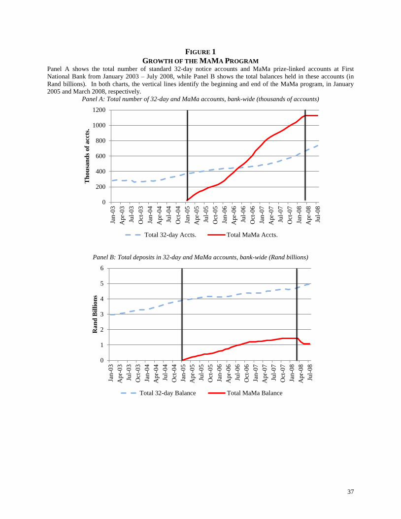
37

FIGURE 1

GROWTH OF THE MAMA PROGRAM Panel A shows the total number of standard 32-day notice accounts and MaMa prize-linked accounts at First

National Bank from January 2003 – July 2008, while Panel B shows the total balances held in these accounts (in

Rand billions). In both charts, the vertical lines identify the beginning and end of the MaMa program, in January

2005 and March 2008, respectively.

Panel A: Total number of 32-day and MaMa accounts, bank-wide (thousands of accounts)

Panel B: Total deposits in 32-day and MaMa accounts, bank-wide (Rand billions)

0

200

400

600

800

1000

1200Ja

n-0

3

Ap

r-0

3

Jul-

03

Oct

-03

Jan

-04

Ap

r-0

4

Jul-

04

Oct

-04

Jan

-05

Ap

r-0

5

Jul-

05

Oct

-05

Jan

-06

Ap

r-0

6

Jul-

06

Oct

-06

Jan

-07

Ap

r-0

7

Jul-

07

Oct

-07

Jan

-08

Ap

r-0

8

Jul-

08

Th

ou

san

ds

of

acc

ts.

Total 32-day Accts. Total MaMa Accts.

0

1

2

3

4

5

6

Jan

-03

Ap

r-0

3

Jul-

03

Oct

-03

Jan

-04

Ap

r-0

4

Jul-

04

Oct

-04

Jan

-05

Ap

r-0

5

Jul-

05

Oct

-05

Jan

-06

Ap

r-0

6

Jul-

06

Oct

-06

Jan

-07

Ap

r-0

7

Jul-

07

Oct

-07

Jan

-08

Ap

r-0

8

Jul-

08

Ra

nd

Bil

lio

ns

Total 32-day Balance Total MaMa Balance

38

FIGURE 2

SHARE OF DEPOSITS HELD IN STANDARD SAVINGS AND PLS, BY AGE AND INCOME Panel A of this figure displays share of total deposits held by individuals in different age brackets for both standard

32-day and MaMa accounts. Panel B shows the share of total balances held by individuals across income brackets.

For reference, the 25th

, 50th

, 75th

, and 95th

percentiles of income in South Africa in 2005 were R13,314, R26,559,

R68,527, and R290,253, respectively. Data reflect account balances as of June 2008, 3 months after the MaMa

program ended.

Panel A: Share of deposits held, by age bracket

Panel B: Share of deposits held, by income bracket

0%

5%

10%

15%

20%

25%

0-21 22-30 31-40 41-50 51-60 61-70 71+

MaMa Standard 32-day

0%

10%

20%

30%

40%

50%

MaMa Standard 32-day

39

FIGURE 3

SHARE OF EMPLOYEES WITH STANDARD SAVINGS OR PLS ACCOUNTS, BY INCOME This figure plots the share of bank employees that have a standard savings account or MaMa account across ten

income deciles. Employees are classified as having a standard savings account if they have either a regular 32-day

notice account or a money market account. Income deciles divide the 38,262 employees into ten groups of 3,826

employees each based on estimated income.

0%

10%

20%

30%

40%

50%

60%

70%

80%

1 2 3 4 5 6 7 8 9 10

Income Decile

MaMa 32-day or Money Market

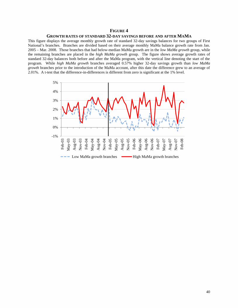
40

FIGURE 4

GROWTH RATES OF STANDARD 32-DAY SAVINGS BEFORE AND AFTER MAMA This figure displays the average monthly growth rate of standard 32-day savings balances for two groups of First

National’s branches. Branches are divided based on their average monthly MaMa balance growth rate from Jan.

2005 – Mar. 2008. Those branches that had below-median MaMa growth are in the low MaMa growth group, while

the remaining branches are placed in the high MaMa growth group. The figure shows average growth rates of

standard 32-day balances both before and after the MaMa program, with the vertical line denoting the start of the

program. While high MaMa growth branches averaged 0.57% higher 32-day savings growth than low MaMa

growth branches prior to the introduction of the MaMa account, after this date the difference grew to an average of

2.01%. A t-test that the difference-in-differences is different from zero is significant at the 1% level.

-1%

0%

1%

2%

3%

4%

5%

Feb

-03

May

-03

Au

g-0

3

No

v-0

3

Feb

-04

May

-04

Au

g-0

4

No

v-0

4

Feb

-05

May

-05

Au

g-0

5

No

v-0

5

Feb

-06

May

-06

Au

g-0

6

No

v-0

6

Feb

-07

May

-07

Au

g-0

7

No

v-0

7

Feb

-08

Low MaMa growth branches High MaMa growth branches

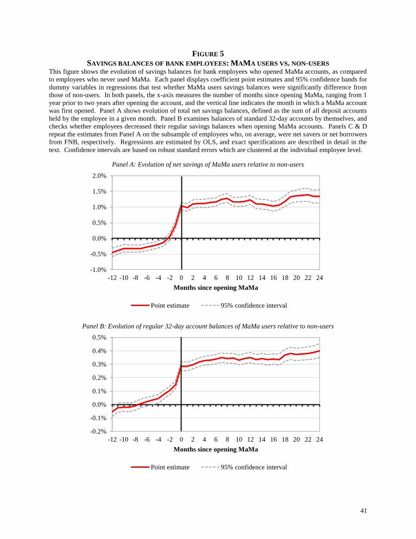
41

FIGURE 5

SAVINGS BALANCES OF BANK EMPLOYEES: MAMA USERS VS. NON-USERS This figure shows the evolution of savings balances for bank employees who opened MaMa accounts, as compared

to employees who never used MaMa. Each panel displays coefficient point estimates and 95% confidence bands for

dummy variables in regressions that test whether MaMa users savings balances were significantly difference from

those of non-users. In both panels, the x-axis measures the number of months since opening MaMa, ranging from 1

year prior to two years after opening the account, and the vertical line indicates the month in which a MaMa account

was first opened. Panel A shows evolution of total net savings balances, defined as the sum of all deposit accounts

held by the employee in a given month. Panel B examines balances of standard 32-day accounts by themselves, and

checks whether employees decreased their regular savings balances when opening MaMa accounts. Panels C & D

repeat the estimates from Panel A on the subsample of employees who, on average, were net savers or net borrowers

from FNB, respectively. Regressions are estimated by OLS, and exact specifications are described in detail in the

text. Confidence intervals are based on robust standard errors which are clustered at the individual employee level.

Panel A: Evolution of net savings of MaMa users relative to non-users

Panel B: Evolution of regular 32-day account balances of MaMa users relative to non-users

-1.0%

-0.5%

0.0%

0.5%

1.0%

1.5%

2.0%

-12 -10 -8 -6 -4 -2 0 2 4 6 8 10 12 14 16 18 20 22 24

Months since opening MaMa

Point estimate 95% confidence interval

-0.2%

-0.1%

0.0%

0.1%

0.2%

0.3%

0.4%

0.5%

-12 -10 -8 -6 -4 -2 0 2 4 6 8 10 12 14 16 18 20 22 24

Months since opening MaMa

Point estimate 95% confidence interval

42

Panel C: Evolution of net savings of MaMa users relative to non-users, employees who are net savers only

Panel D: Evolution of net savings of MaMa users relative to non-users, employees who are net borrowers only

0.0%

0.5%

1.0%

1.5%

2.0%

2.5%

3.0%

-12 -10 -8 -6 -4 -2 0 2 4 6 8 10 12 14 16 18 20 22 24

Months since opening MaMa

Point Estimate 95% confidence interval

-1.5%

-1.0%

-0.5%

0.0%

0.5%

1.0%

1.5%

-12 -10 -8 -6 -4 -2 0 2 4 6 8 10 12 14 16 18 20 22 24

Months since opening MaMa

Point Estimate 95% confidence interval

43

FIGURE 6

EFFECT OF JACKPOT PRIZE WINNER ON LOCAL MAMA DEMAND This figure shows the impact of having a million-Rand prize winner on local MaMa demand. Each panel displays

coefficient point estimates and 95% confidence bands from seven separate regressions which test the lead and lag

effect of a jackpot win. Panel A shows the effect of having a million-Rand winner on the excess monthly growth

rate of MaMa balances at the same branch, relative to all other bank branches. Panels B and C are similar, except

they show the impact of a jackpot win on the change in the number of MaMa accounts and the total standard 32-day

deposits at the branch, respectively. Panel D displays the spillover effect of a jackpot win on the growth rate of

MaMa balances at branches that are within 10km of the winning branch. Regressions are estimated by OLS, and

exact specifications are described in detail in the text. Confidence intervals are based on robust standard errors

which are clustered at the branch level.

Panel A: Excess growth of total MaMa deposits at winning branch

Panel B: Change in number of MaMa accounts at winning branch

-20%

-15%

-10%

-5%

0%

5%

10%

15%

20%

-3 -2 -1 0 1 2 3

Months since winner

Point estimate 95% confidence interval

-60

-40

-20

0

20

40

60

80

-3 -2 -1 0 1 2 3

Point estimate 95% confidence interval

44

FIGURE 6 - continued

Panel C: Excess growth of total 32-day deposits at winning branch

Panel D: Excess growth of total MaMa deposits at nearby branches

-4%

-2%

0%

2%

4%

6%

8%

-3 -2 -1 0 1 2 3

Point estimate 95% confidence interval

-6%

-4%

-2%

0%

2%

4%

6%

8%

-3 -2 -1 0 1 2 3

Point estimate 95% confidence interval

45

TABLE I

SUMMARY STATISTICS OF FIRST NATIONAL BANK DATA

This table reports summary statistics for data obtained from First National Bank. Panel A presents summary

statistics on the total number of accounts and total deposits in standard 32-day and MaMa accounts at 604 bank

branches as of March 2008, when the MaMa program ended. Panel B compares the share of balances owned by

race and gender for 32-day and MaMa accounts. Panel C contains account-level summary statistics for bank

employees.

Panel A: Branch-level summary statistics as of March 2008

Product N Mean

Std.

Dev.

10th

percentile Median

90th

percentile

Total No. of Accounts 32-day 604 1,097 1,064 148 826 2,273

MaMa 604 1,863 2,505 211 1,408 3,797

Total balance (Rand millions) 32-day 604 R 7.81 R 8.08 R 0.89 R 5.29 R 18.00

MaMa 604 R 2.35 R 3.25 R 0.23 R 1.70 R 5.00

Panel B: Share of balances owned by race and gender

MaMa 32-day

Race:

Black 0.45 0.45

White 0.37 0.41

Asian 0.09 0.07

Mixed race 0.08 0.07

Males 0.52 0.46

Panel C: Account-level summary statistics of bank employees as of March 2008

N Mean

Std.

Dev.

10th

%tile Median

90th

%tile

% with non-zero

balance

Jan.

2005

Mar.

2008

Total balance:

32-day saving 38,301 872 9,989 0 0 322 9.9% 15.4%

Money market 38,301 3,285 31,091 0 0 841 -- 22.9%

Checking 38,301 206 17,507 -5,833 0 2,703 39.0% 62.6%

MaMa 38,301 567 5,510 0 0 723 5.5% 45.5%

Combined 38,301 4,930 39,921 -5,065 0 10,043 41.4% 77.9%

Income Estimate 38,301 175,920 203,408 60,000 112,297 360,000 -- --

Combined bal. (% income) 38,301 3.41 62.44 -4.4 0 6.9 -- --

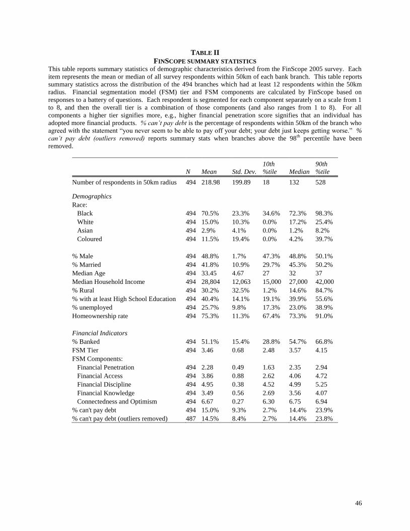
46

TABLE II

FINSCOPE SUMMARY STATISTICS This table reports summary statistics of demographic characteristics derived from the FinScope 2005 survey. Each

item represents the mean or median of all survey respondents within 50km of each bank branch. This table reports

summary statistics across the distribution of the 494 branches which had at least 12 respondents within the 50km

radius. Financial segmentation model (FSM) tier and FSM components are calculated by FinScope based on

responses to a battery of questions. Each respondent is segmented for each component separately on a scale from 1

to 8, and then the overall tier is a combination of those components (and also ranges from 1 to 8). For all

components a higher tier signifies more, e.g., higher financial penetration score signifies that an individual has

adopted more financial products. % can’t pay debt is the percentage of respondents within 50km of the branch who

agreed with the statement “you never seem to be able to pay off your debt; your debt just keeps getting worse.” %

can’t pay debt (outliers removed) reports summary stats when branches above the 98th

percentile have been

removed.

N Mean Std. Dev.

10th

%tile Median

90th

%tile

Number of respondents in 50km radius 494 218.98 199.89 18 132 528

Demographics

Race:

Black 494 70.5% 23.3% 34.6% 72.3% 98.3%

White 494 15.0% 10.3% 0.0% 17.2% 25.4%

Asian 494 2.9% 4.1% 0.0% 1.2% 8.2%

Coloured 494 11.5% 19.4% 0.0% 4.2% 39.7%

% Male 494 48.8% 1.7% 47.3% 48.8% 50.1%

% Married 494 41.8% 10.9% 29.7% 45.3% 50.2%

Median Age 494 33.45 4.67 27 32 37

Median Household Income 494 28,804 12,063 15,000 27,000 42,000

% Rural 494 30.2% 32.5% 1.2% 14.6% 84.7%

% with at least High School Education 494 40.4% 14.1% 19.1% 39.9% 55.6%

% unemployed 494 25.7% 9.8% 17.3% 23.0% 38.9%

Homeownership rate 494 75.3% 11.3% 67.4% 73.3% 91.0%

Financial Indicators

% Banked 494 51.1% 15.4% 28.8% 54.7% 66.8%

FSM Tier 494 3.46 0.68 2.48 3.57 4.15

FSM Components:

Financial Penetration 494 2.28 0.49 1.63 2.35 2.94

Financial Access 494 3.86 0.88 2.62 4.06 4.72

Financial Discipline 494 4.95 0.38 4.52 4.99 5.25

Financial Knowledge 494 3.49 0.56 2.69 3.56 4.07

Connectedness and Optimism 494 6.67 0.27 6.30 6.75 6.94

% can't pay debt 494 15.0% 9.3% 2.7% 14.4% 23.9%

% can't pay debt (outliers removed) 487 14.5% 8.4% 2.7% 14.4% 23.8%

47

TABLE III

INDIVIDUAL-LEVEL MAMA TAKE-UP AMONG BANK STAFF This table presents estimates from OLS regressions run on the First National Bank staff dataset. In each regression,

the dependent variable equals one if the employee has a positive balance in a particular saving product at any time

during the sample period (Jan. 2005 - Mar. 2008). In Panel A we correlate demographic characteristics with the

propensity to have either a standard 32-day savings account, a money market or standard 32-day account, or a

MaMa account. Ex-staff indicate employees whose employment terminated at some point during the sample period.

In Panel B we test whether previous banking behavior is correlated with the propensity to open a MaMa account,

after controlling for all demographic characteristics contained in Panel A. High and low savings before MaMa are

dummy variables indicating employees with above- and below-median savings, respectively, as a percent of income

prior to opening a MaMa account. High and low borrowing before MaMa are defined similarly for net borrowers

(and thus those with no accounts are the omitted group). All regressions contain 34 bank region fixed effects

(regions are defined internally by First National Bank). Robust standard errors (reported in parentheses) are

clustered at the region level. ***, **, * indicate significance at the 1%, 5%, and 10% level, respectively.

Panel A: Demographic characteristics

Dependent Variable:

Has 32-day

Savings

Account

Has 32-day

or MM

account

Has

MaMa

Account

Age (<30 omitted):

30-39 -0.074*** -0.093*** 0.056***

(0.005) (0.005) (0.011)

40+ -0.096*** -0.104*** 0.146***

(0.009) (0.007) (0.017)

Income decile (1st omitted):

2nd

0.058*** 0.095*** 0.105***

(0.011) (0.010) (0.013)

3rd

0.087*** 0.141*** 0.153***

(0.013) (0.013) (0.016)

4th

0.106*** 0.148*** 0.190***

(0.015) (0.011) (0.010)

5th

0.107*** 0.143*** 0.203***

(0.015) (0.014) (0.012)

6th

0.082*** 0.129*** 0.182***

(0.009) (0.011) (0.013)

7th

0.083*** 0.141*** 0.178***

(0.018) (0.015) (0.012)

8th

0.058*** 0.126*** 0.174***

(0.010) (0.012) (0.012)

9th

0.046*** 0.099*** 0.168***

(0.016) (0.017) (0.014)

10th 0.018 0.064*** 0.145***

(0.015) (0.017) (0.019)

Male -0.061*** -0.088*** -0.042***

(0.004) (0.005) (0.005)

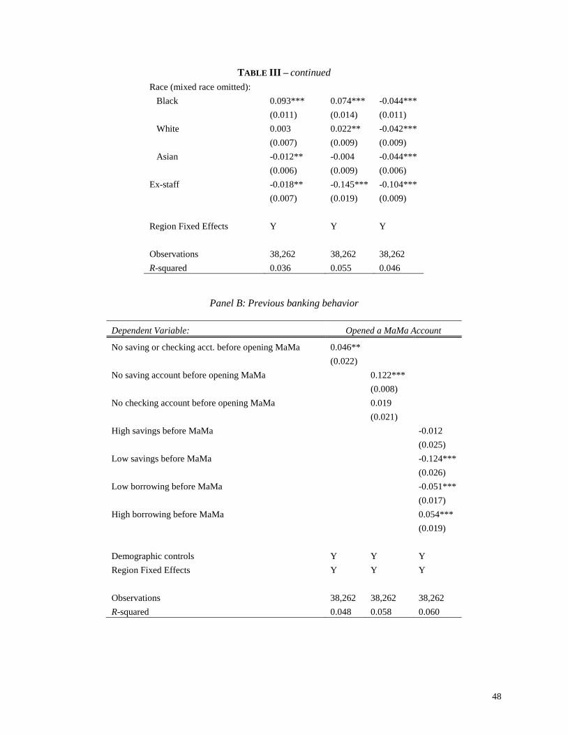
48

TABLE III – continued

Race (mixed race omitted):

Black 0.093*** 0.074*** -0.044***

(0.011) (0.014) (0.011)

White 0.003 0.022** -0.042***

(0.007) (0.009) (0.009)

Asian -0.012** -0.004 -0.044***

(0.006) (0.009) (0.006)

Ex-staff -0.018** -0.145*** -0.104***

(0.007) (0.019) (0.009)

Region Fixed Effects Y Y Y

Observations 38,262 38,262 38,262

R-squared 0.036 0.055 0.046

Panel B: Previous banking behavior

Dependent Variable: Opened a MaMa Account

No saving or checking acct. before opening MaMa 0.046**

(0.022)

No saving account before opening MaMa

0.122***

(0.008)

No checking account before opening MaMa

0.019

(0.021)

High savings before MaMa

-0.012

(0.025)

Low savings before MaMa

-0.124***

(0.026)

Low borrowing before MaMa

-0.051***

(0.017)

High borrowing before MaMa

0.054***

(0.019)

Demographic controls Y Y Y

Region Fixed Effects Y Y Y

Observations 38,262 38,262 38,262

R-squared 0.048 0.058 0.060

49

TABLE IV

BRANCH-LEVEL MAMA TAKE-UP AS A FUNCTION OF DEMOGRAPHIC AND FINANCIAL

CHARACTERISTICS This table presents results of OLS regressions where the dependent variable is the log total usage of MaMa in March

2008 (at the close of the program) for each bank branch. Panel A shows the relationship between demographic

characteristics and MaMa usage, as measured both by log total MaMa deposits and by the log number of MaMa

accounts. Panel B adds financial characteristics to these demographic controls to test whether banking attitudes

have an additional impact on MaMa usage. To be concise, we present only results relating to log total MaMa

deposits in Panel B, but similar results are found using log number of MaMa accounts. Independent variables come

from the FinScope 2005 survey, and are averages (or medians, if specified) for all respondents within a 50km radius

of the bank branch. FSM Tier is a classification created by FinScope which categorizes respondents by various

financial segments, and is based on 5 separate components which are identified separately in Panel B. See text for a

complete explanation of how the FSM tiers were created. The final column of Panel B removes branches above the

98th

percentile of % can’t pay debt. In all regressions we control for the size of the branch by including the log total

amount of regular 32-day deposits as an independent variable. Standard errors are clustered by 54 district

municipalities, and are reported in parentheses. ***, **, and * indicate significance at the 1%, 5%, and 10% level,

respectively.

Panel A: Demographic characteristics

Dependent variable:

Ln(MaMa

deposits)

Ln(No. of

MaMa

accts.)

Race (% Coloured omitted):

% Black -0.560** -0.869***

(0.267) (0.205)

% White -0.188 -0.753

(0.660) (0.591)

% Asian 3.343*** 3.986***

(0.748) (0.682)

% Male 1.500 0.423

(1.771) (1.748)

% Married -0.169 -0.158

(0.279) (0.317)

Median Age -0.009 -0.004

(0.007) (0.009)

Median Household Income -0.005 -0.003

(0.004) (0.003)

% with at least High School education 0.510 0.236

(0.362) (0.367)

Unemployment rate -0.572 -0.169

(0.472) (0.407)

Homeownership rate -0.594* -0.490

(0.299) (0.315)

Rural Area -0.342 -0.291

(0.212) (0.207)

Ln(Regular savings demand) 0.796*** 0.856***

(0.034) (0.037)

Observations 494 494

R-squared 0.772 0.754

50

TABLE IV - continued

Panel B: Financial characteristics

Full Sample

Outliers

removed

Dependent variable: Ln(MaMa deposits)

% banked -0.495

(0.411)

FSM Tier

-0.122

(0.158)

FSM Components:

Financial Penetration

-0.385**

(0.191)

Financial Access

0.080

(0.081)

Financial Discipline

-0.131

(0.114)

Financial Knowledge

0.255

(0.156)

Connectedness and Optimism

-0.350***

(0.126)

% can't pay off debt

0.742

1.685***

(0.550)

(0.433)

Demographic controls Y Y Y Y

Y

Observations 494 494 494 494

487

R-squared 0.773 0.773 0.781 0.775 0.777

51

TABLE V

BANK-WIDE MAMA GROWTH AND THE NATIONAL LOTTERY This table relates overall MaMa demand to the size of the jackpot available in the South Africa National Lottery.

Each week, winning lotto numbers are drawn on Wednesday and Saturday. For each regression, the dependent

variable is an indicator of growth in MaMa usage over the 3-day period (M-W or Th-S) preceding the draw. ln(New

funds deposited) is the log of total Rand deposited in new accounts during the draw period , and # of new accts.

opened is the total number of new MaMa accounts opened over the draw period. Jackpot sizes were estimated and

published by the National Lottery prior to the draw. We non-parametrically divide jackpots into 4 quartiles, where

the largest jackpots are typically due to rollovers or guaranteed prizes. Saturday indicates draws that were done on

Saturday, and controls for time-of-week fixed effects. Few business days controls for draw periods that covered less

than 3 business days due to holidays. Savings growth controls for the growth in regular 32-day deposit balances (1st

column) and accounts (2nd

column) at First National during the draw period. To remove serial correlation, we

include lagged values of the dependent variable. In addition, 4 time fixed effects are included to control for different

periods of the MaMa program: Jan-Sept. 2005, Oct. 2005-Jun. 2006, Jul. 2006-Mar. 2007, and the period after the

lottery re-opened from Oct. 2007-Mar. 2008. Newey-West standard errors that account for up to 2 weeks of

remaining serial correlation are reported. ***, **, * indicate significance at the 1%, 5%, and 10% levels,

respectively.

Dependent Variable:

ln(New funds

deposited)

# of new

accts. opened

Estimated Jackpot size (< R3 million omitted)

R3 million - R4 million -0.0140

-121.0

(0.0705)

(151.9)

R4 million - R7 million -0.149***

-382.6***

(0.0473)

(130.7)

> R7 million -0.155***

-315.8**

(0.0589)

(159.1)

Saturday -0.0602

74.67

(0.0460)

(99.79)

Few Business days -0.409***

-1,189***

(0.0893)

(170.2)

Savings Growth (%) 3.045

13,347**

(2.564)

(5,794)

Lagged dependent variable 0.672***

0.693***

(0.0578)

(0.0567)

Time period fixed effects Y

Y

Observations 276 276

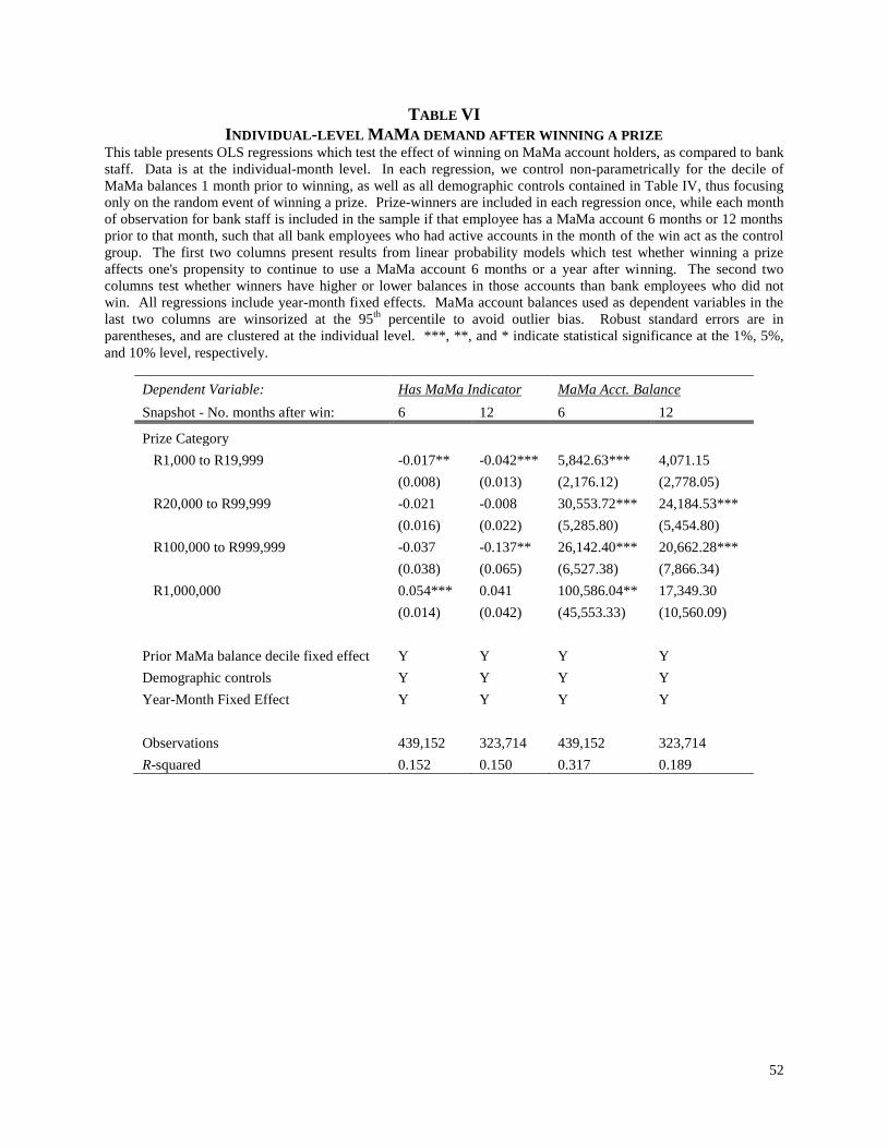
52

TABLE VI

INDIVIDUAL-LEVEL MAMA DEMAND AFTER WINNING A PRIZE This table presents OLS regressions which test the effect of winning on MaMa account holders, as compared to bank

staff. Data is at the individual-month level. In each regression, we control non-parametrically for the decile of

MaMa balances 1 month prior to winning, as well as all demographic controls contained in Table IV, thus focusing

only on the random event of winning a prize. Prize-winners are included in each regression once, while each month

of observation for bank staff is included in the sample if that employee has a MaMa account 6 months or 12 months

prior to that month, such that all bank employees who had active accounts in the month of the win act as the control

group. The first two columns present results from linear probability models which test whether winning a prize

affects one's propensity to continue to use a MaMa account 6 months or a year after winning. The second two

columns test whether winners have higher or lower balances in those accounts than bank employees who did not

win. All regressions include year-month fixed effects. MaMa account balances used as dependent variables in the

last two columns are winsorized at the 95th

percentile to avoid outlier bias. Robust standard errors are in

parentheses, and are clustered at the individual level. ***, **, and * indicate statistical significance at the 1%, 5%,

and 10% level, respectively.

Dependent Variable: Has MaMa Indicator MaMa Acct. Balance

Snapshot - No. months after win: 6 12 6 12

Prize Category

R1,000 to R19,999 -0.017** -0.042*** 5,842.63*** 4,071.15

(0.008) (0.013) (2,176.12) (2,778.05)

R20,000 to R99,999 -0.021 -0.008 30,553.72*** 24,184.53***

(0.016) (0.022) (5,285.80) (5,454.80)

R100,000 to R999,999 -0.037 -0.137** 26,142.40*** 20,662.28***

(0.038) (0.065) (6,527.38) (7,866.34)

R1,000,000 0.054*** 0.041 100,586.04** 17,349.30

(0.014) (0.042) (45,553.33) (10,560.09)

Prior MaMa balance decile fixed effect Y Y Y Y

Demographic controls Y Y Y Y

Year-Month Fixed Effect Y Y Y Y

Observations 439,152 323,714 439,152 323,714

R-squared 0.152 0.150 0.317 0.189