Can exchange traded funds be used to exploit

country and industry momentum?1

Laura Andreu University of Zaragoza

landreu@unizar.es

Laurens Swinkels Erasmus Research Institute of Management

Robeco Investments

lswinkels@ese.eur.nl

Liam Tjong-A-Tjoe Lazard

Liam.TjongATjoe@lazard.com

January 2011

1 The views expressed in this paper are those of the authors and do not necessarily represent the views of the companies they are affiliated with. This paper was written when Andreu was a visiting scholar at Erasmus School of Economics and Tjong-A-Tjoe was affiliated with Erasmus School of Economics.

2

Can exchange traded funds be used to exploit

industry and country momentum?

ABSTRACT

There is overwhelming empirical evidence on the existence of country and industry

momentum effects. This line of research suggests that investors who buy countries and

industries with relatively high past returns and sell countries and industries with relatively low

past returns will earn positive risk-adjusted returns. These studies focus on country and

industry indexes that cannot be traded directly by investors. This warrants the question

whether country and industry momentum effects can really be exploited by investors or are

illusionary in nature. We analyze the profitability of country and industry momentum

strategies using actual price data on Exchange Traded Funds. We find that, over the sample

periods that these ETFs were traded, an investor would have been able to exploit country and

industry momentum strategies with an excess return of about 5% per annum. The daily

average bid-ask spreads on ETFs are substantially below the implied break-even transaction

costs levels. Hence, we conclude that investors that are not willing or able to trade individual

stocks are able to use ETFs to benefit from momentum effects in country and industry

portfolios.

Keywords: Alpha, Country momentum strategies, Exchange traded funds, Industry

momentum strategies, Transactions costs

JEL Codes: C53, G11, G12

3

1. Introduction The medium-term momentum effect, initially documented by Jegadeesh and Titman (1993),

has generated much interest from academia as well as investment professionals. While

academia has tried to understand the source and nature of this effect, many investment

professionals are concerned with the question whether it is possible to implement momentum

strategies in practice to generate excess returns for themselves or their clients.2 Investing in a

momentum strategy is cumbersome for investors, as it requires monthly buying and short-

selling of many individual stocks.3 It would be much more convenient for investors if

momentum would also be present in aggregated return series that can be traded more easily;

such as country or industry portfolios.

Bhojraj and Swaminathan (2006) indicate that country momentum profits can be earned by

buying stock market indexes of countries with high past returns and selling country indexes

with low past returns. Similarly, Moskowitz and Grinblatt (1999) report that most of the

momentum effect measured on the individual stock level can be captured by following an

industry momentum strategy. They base their industry portfolios on industry classifications

that are not tradable. Hence, investors who would like to follow this strategy are still required

to buy and short-sell individual stocks. O’Neal (2000) investigates whether industry

momentum is also present in tradable industry assets by evaluating the existence of industry

mutual fund momentum. He finds a significant excess return of 7.5% per annum over the

period 1989 to 1999 for past winner industry mutual funds over past loser industry mutual

funds even after accounting for the initial loads and redemption fees. However, he concludes

long-only investors cannot improve their risk-adjusted performance by following an industry

momentum strategy using industry mutual funds.

Using industry mutual funds to exploit the momentum effect has some disadvantages. O’Neal

(2000) notes that the industry mutual funds he uses are actively managed. Hence, it is not

2 See Swinkels (2004) for an overview on research on momentum investing. Pettengill, Edwards, and Schmitt (2006) suggest that momentum strategies a not viable for individual investors. 3 As far as we know, private investors do not have the opportunity to follow an individual momentum strategy by purchasing a mutual fund or exchange traded fund that solely focuses on this strategy. The AQR Momentum Fund (AMOMX) is a notable exception, but requires at least $5 million as an initial investment (source: Morningstar). .

4

clear whether the 7.5% per annum relative performance is due to industry momentum or

mutual fund portfolio manager skill. The use of index mutual funds would alleviate this

problem to a certain extent, but it is hardly possible to short-sell mutual funds, which is

required if investors would like to follow the long-short industry momentum strategy. Hence,

our analysis focuses on Exchange Traded Funds (ETFs), which do not suffer from these

disadvantages.4 ETFs are designed to passively mimic a predefined index by construction, are

less effected by capital gains tax, and can be sold short relatively easy, which makes them a

more suitable candidate for implementing momentum strategies than mutual funds.

The contribution of this paper is twofold. First, we investigate whether the country and

industry momentum effects are present in tradable securities that have the objective to mimic

country and industry indexes. We find that over the period ETFs are available they have been

able to generate country and industry momentum returns that are economically as large as

those calculated before using non-tradable indexes. Second, we use daily data on bid-ask

spreads of country and industry ETFs to gauge the importance of transaction costs on the real-

life returns that investors following these strategies might earn. We find that bid-ask spreads

are substantially smaller than break-even levels of transaction costs for the ETF-based

momentum strategies. Our results imply that country and industry momentum effects are not

illusionary, but can be captured by investors not willing or able to trade each individual stock

separately. Another implication is that asset managers employing trading strategies that are

country or industry neutral do not make use of a viable source of additional return.

The setup of this paper is as follows. In Section 2, we analyze the paper profitability of

country and industry momentum strategies. In Section 3, we introduce ETFs and their

advantages and disadvantages over mutual funds. In Section 4, we indicate how to translate

the paper momentum profits into real-life trading profits by using ETFs and taking into

account transactions costs. Section 5 concludes.

2. The profitability of momentum strategies In this section we start by explaining the methodology that we follow to construct momentum

portfolios. Then we proceed to examine US industry momentum over the period 1926-2009.

4 De Jong and Rhee (2008) also investigate momentum effects using ETFs. However, they investigate momentum across asset classes instead of country and industry momentum within equity markets.

5

Next, we investigate the existence of country momentum at the country index level over the

period 1970 to 2009.

2.1 Portfolio construction methodology

We use the portfolio composition technique as also employed by Jegadeesh and Titman

(1993). Using different combinations of J formation periods and K investment periods we test

16 different strategies, with J and K taking values of 3, 6, 9 or 12 months.

Let us, for expositional purposes, assume that we follow a (6,6) strategy, meaning that both J

and K are 6 months. We also assume that our strategy takes a long position in the single best

performing asset and a short position in the single worst performing asset. The investment

procedure is as follows: at t = 0 we consider the investment objects that are available (the

industry or country indices) and rank them based on their performance over the last 6 months.

Then, at t = 0, we invest 1/6 of the amount of total capital in the best performing index based

on their performance in the 6 months directly preceding the investment. The amount of capital

that we want exposed does not have very stringent restrictions as this investment is financed

by selling short exactly the same amount of the worst performing index. After the first month

we do this again and keep doing this for 6 months. This means that after 6 months we have

put in the full amount of capital in our long position and financed this amount by our short

position. Now, after 6 months, we liquidate the investment made at t = 0. For the long

position this means that we sell 1/6 of our initial capital of the investment object that we

invested in K months ago plus (minus) the growth (loss) that the position encountered during

those months.

2.2 Industry momentum

In this subsection we show that industry momentum strategies based on non-tradable indexes

have historically been profitable with both economic and statistical significance.5 We start by

investigating the industry classification from the Kenneth French on-line data library. These

indices together cover all the stocks from the NYSE, AMEX and NASDAQ. They are sorted

into 10 portfolios based on their 4 digit SIC code. The index returns are based on the market

capitalization weighted returns of the individual assets. We use data for the period July 1926 5 In this paper we focus on U.S. industry momentum. Swinkels (2002) shows that industry momentum strategies are also profitable when using non-tradable industry indices provided by Thomson Financial for the U.S. and Europe, and to a lesser extent Japan. Giannikos and Ji (2007) investigate industry momentum strategies for many more countries and regions, and conclude that industry momentum is globally present.

6

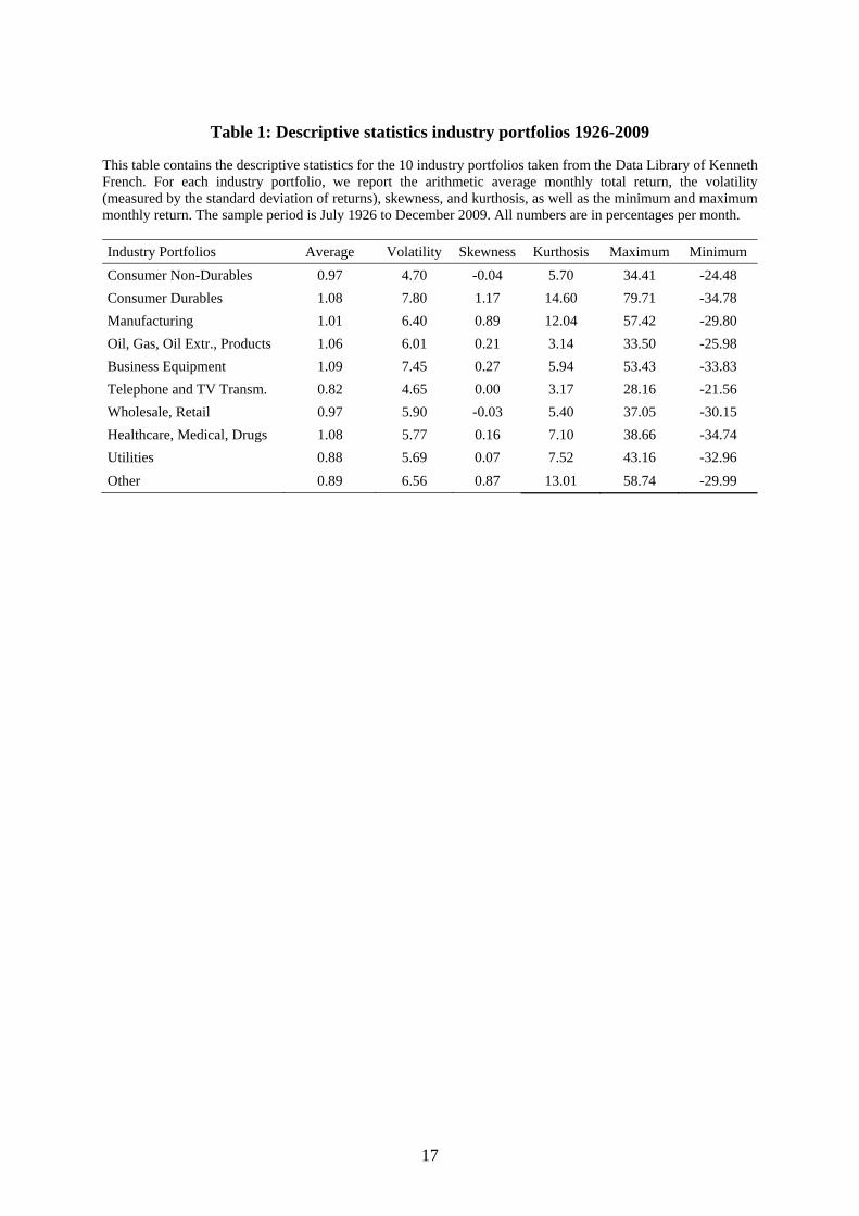
to December 2009. In Table 1 the descriptive statistics of these 10 industry portfolio can be

seen. The average returns are between 0.8% and 1.1% per month for each of the industries,

while standard deviations vary between 4.6% and 7.8% per month.

Once the descriptive statistics of our dataset have been shown, we investigate the presence of

industry momentum. Panel A of Table 2 contains the results of the industry momentum

strategy on the 10 industry portfolios over the period 1926 to 2009. For each of the

observation and holding periods the industry momentum returns are positive. For example,

the short-term (3,3) strategy generates a 0.26% per month excess return. Even on a sample of

more than 80 years, this excess return is not statistically significant at the 5% level. However,

the medium-term momentum strategies show strong statistical significance with t-values well

above two. For example, the medium (6,6) strategy has an excess return of 0.43% per month

with a t-statistic of 2.65 indicating statistical significance. For longer holding periods, the

industry momentum return is again lower. The magnitude of the industry momentum profits is

similar to the figures reported in Moskowitz and Grinblatt (1999), who investigate industry

momentum over the period 1965 to 1995. They coincidentally also report 0.43% excess return

for their medium-term industry momentum strategy. The (12,12) industry momentum strategy

in their study has a somewhat higher excess return, with 0.26% per month versus the 0.12%

per month that we find. Panel B of Table 2 suggests that when the Winner and Loser portfolio

contain three industry portfolios instead of one, the excess returns are still statistically

significant, but with a lower economic magnitude. For example, the (6,6) strategy now has an

excess return of 0.27% per month instead of 0.43% per month. In Panel C of Table 2 we see

that, when all US stocks are divided in 30 industry portfolios and the Winner and Loser

portfolio contain the three industry portfolios with highest and lowest past return, the excess

returns are economically and statistically significant.

2.3 Country momentum

In addition to industry momentum, research on international equity markets has extensively

investigated the presence of momentum at the country index level. For example, Richards

(1997), Chan, Hameed, and Tong (2000), and Bhojraj and Swaminathan (2006) all find

7

country momentum to be profitable investment strategies.6 Indeed, also these authors do not

directly test these strategies on tradable assets, but use non-tradable calculated indexes

instead. Table 3 contains the descriptive statistics of our country indexes from Morgan

Stanley Capital International (MSCI) over the period 1970 to 2009. The average returns are

between 0.79% and 1.75% per month for each of the countries, while standard deviations vary

between 4.5% and 10.4% per month.

Next, we extend the country momentum analysis from Bhojraj and Swaminathan (2006) using

a sample of non-tradable country indexes over the period 1970 to 2009. Table 4 contains the

momentum profits from formation and investment periods ranging from 3 to 12 months based

on 16 country indexes. Panel A of Table 4 contains the results for momentum strategies that

take a long and short position in a single country index. This panel indicates substantial

profits from country momentum trading on the medium term. The (6,6) country momentum

strategy returns a statistically significant 0.73% per month return. This is almost double the

industry momentum return analyzed in the previous section. For shorter and longer formation

and holding periods the returns are somewhat weaker and less often statistically significant.

Our results are in line with those by Bhojraj and Swaminathan (2006). They also report a

0.7% per month return on a strategy that ranks countries from developed markets based on

US$ returns. In Panel B of Table 4 we also investigate the excess returns when we take the

three countries with highest and lowest momentum, instead of the single country approach in

Panel A. We see that for the (6,6) strategy the average excess return is virtually the same as in

Panel A, but since we obtain some country diversification, t-values are substantially higher for

such strategy.

3. Exchange Traded Funds In this section we explain in more detail what an Exchange Traded Fund (ETF) is and why

ETFs are particularly useful for investors that want to trade a group of securities, such as an

industry or country portfolio, with just one trade. We also discuss the differences with more

traditional assets such as mutual funds.

6 Nijman, Swinkels, and Verbeek (2004) report that for momentum strategies within Europe, country momentum is virtually non-existent once industry momentum effects are taken into account.

8

3.1 What is an Exchange Traded Fund? Exchange Traded Funds (ETFs) pool together a set of individual underlying assets in such a

way that they can be securitized (i.e. converted into tradable assets). Usually ETFs are used to

provide a tradable security that mimics the results and thus the composition of a certain index.

If an investor wants to put his or her money in that index (e.g. the S&P500) they can buy an

ETF instead of having to buy all the underlying assets that are included in that index (e.g. the

500 stocks in the S&P500, correctly weighted). An ETF is then traded on a stock exchange,

just like any other regular stock. With the creation of this relatively new investment tool a

new opportunity is created for investors to easily diversify their investment portfolio.

At the end of the 1970s, stock brokers started offering investors the possibility to place a

single order to buy an entire portfolio of stocks (at that time consisting usually of all the

stocks of the S&P500; Gastineau 2001). This development led to the interest of smaller

investors for opportunities to achieve the same level of diversification in an easy way without

having to buy the actual 500 shares. After the development of a couple of somewhat complex

structures with this goal, the first ETF was introduced in 1993. The American Stock Exchange

(Amex) developed the Standard and Poor’s Depository Receipt (SPDR, commonly referred to

as “spiders”), a Unit Investment Trust structure (UIT) tracking the S&P500 index.

The UIT, together with the Open-End Structure, is one of the two common legal structures

that are used for ETFs. The main difference between a UIT and an open-end fund is that

dividends related to the underlying stocks are paid out to investors under a UIT structure

while under an open-end structure they are reinvested in underlying stock. Dividends under a

UIT are deposited in a non-interest bearing account until actual distribution, thus creating a

‘cash drag’.

3.2 How ETFs Work in Comparison to Mutual Funds

An ETF is initiated as follows: individual assets like stocks or bonds are acquired by the

initiator (the market maker) and set aside. The number of assets is usually quite high such that

the number of ETF shares that can be distributed is in the range of a couple of ten-thousands.

The market maker can now sell the ETFs to the market where they are subsequently traded

secondarily just like any other tradable security.

9

The reverse process of creation takes place upon redemption. ETFs can be removed from the

market by the owner if he has sufficient units to claim a set of underlying assets that were set

aside. He then trades in his ETFs against one complete set of the underlying assets. This is

called ‘redemption in kind’. As pointed out by Gastineau (2001), the fact that market

participants can redeem at any time (given that they have enough shares) ensures that the

trading price of an ETF correctly resembles the Net Asset Value (NAV) of the underlying

assets. If the price of an ETF is significantly higher than the value of the underlying stocks,

market makers will try to profit by buying more of those stocks on the market (at the low

price), creating ETFs and selling those at the high price. The opposite happens when the ETF

price drops too low; Poterba and Shoven (2002). Changes in supply and demand due to

arbitrage possibilities will then move the ETF price back to NAV.

An ETF in some respect resembles a mutual fund: the owner has a stake in a pool of

underlying assets and is therefore entitled to a share in the returns of that pool. There are some

key aspects however that set ETFs apart. It has to be pointed out that the mutual fund universe

is very diverse and that some of these funds are less comparable with ETFs than others,

specifically: mutual funds that are actively managed by a fund manager. The goal of an ETF

is to track an existing index and thus active management of the composition of the underlying

assets does not fit in the ETF concept. The so-called open-end index mutual funds share this

passive attitude and will therefore be our framework for comparison. Generally we recognize

three important differences.

First, considered of the most important characteristics of ETFs that they not share with index

mutual funds is the fact that they can be actively traded on the market. Mutual fund shares can

only be bought and sold directly from and to the issuer. Also, mutual funds have a single point

in the day where the NAV of the fund is established (usually at 4:00pm, at the end of the

trading day) that determines the price that is used in a trade. This is not the case with ETFs,

whose prices constantly change during trading as a result of supply and demand forces.

Because of this, ETFs are a more efficient tool for traders that regularly act on intraday

information.

A second advantage of the fact that ETFs are traded just like stocks is that they can be sold

short. This is not the case with mutual funds which might drive an ETF’s appeal over their

10

mutual fund counterpart in some situations as well. We see later that this is in fact an essential

part of momentum trading.

The third major difference is the tax implication of ETFs compared to mutual funds. We

mentioned that ETFs can be redeemed in kind. This is not possible with mutual funds, where

redemption takes place in cash. The potential tax benefit of ETFs is then created in two ways.

Agapova (2011) argues that mutual funds will often sell a part of the portfolio in order to

create liquidity to pay the investors that redeem. If the fund sells assets that have increased in

value since their acquisition a taxable capital gain is created for all investors that take part in

that mutual fund. This means that investors do not have control over this part of taxable gains.

ETFs do not have this problem. The second potential benefit is that investors who decide to

redeem their ETFs do not generate a taxable capital gain because of the fact that they just

receive the basket of underlying assets. Taxation is postponed to a later date where they

decide to sell those stocks; Poterba and Shoven (2002).

4. Momentum profits using tradable assets In this section we investigate whether the excess returns calculated using non-tradable country

and industry portfolios can be captured when tradable ETFs are used. We also attempt to

gauge the effect of transaction costs by analyzing the bid-ask spread on these ETFs in more

detail.

4.1 Do tradable country or industry indexes exhibit momentum?

Our goal is to find out if it is possible to set up a strategy that can translate the industry

momentum effect as found by Moskowitz and Grinblatt (1999) and country momentum effect

as in Bhojraj and Swaminathan (2006) into real-life profits for investors. If the effect truly

exists, we should find that the industries or countries that have performed well in the past 3 to

12 months will continue to do so in the coming 3 to 12 months. Since neither the industry

portfolios of Moskowitz and Grinblatt (1999), nor the Kenneth French industry portfolios

used in Section 2 are directly tradable instruments, we consider a set of ETFs that track

industry indices as our investment universe. One of the main advantages of using ETFs as

opposed to individual stocks belonging to the same industry is that it drastically reduces the

number of trades in a strategy, which impacts the amount of trading and the magnitude of

11

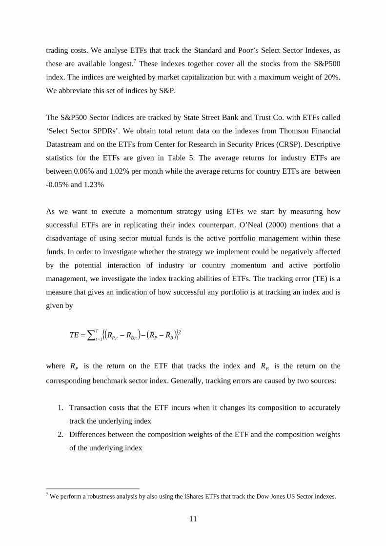
trading costs. We analyse ETFs that track the Standard and Poor’s Select Sector Indexes, as

these are available longest.7 These indexes together cover all the stocks from the S&P500

index. The indices are weighted by market capitalization but with a maximum weight of 20%.

We abbreviate this set of indices by S&P.

The S&P500 Sector Indices are tracked by State Street Bank and Trust Co. with ETFs called

‘Select Sector SPDRs’. We obtain total return data on the indexes from Thomson Financial

Datastream and on the ETFs from Center for Research in Security Prices (CRSP). Descriptive

statistics for the ETFs are given in Table 5. The average returns for industry ETFs are

between 0.06% and 1.02% per month while the average returns for country ETFs are between

-0.05% and 1.23%

As we want to execute a momentum strategy using ETFs we start by measuring how

successful ETFs are in replicating their index counterpart. O’Neal (2000) mentions that a

disadvantage of using sector mutual funds is the active portfolio management within these

funds. In order to investigate whether the strategy we implement could be negatively affected

by the potential interaction of industry or country momentum and active portfolio

management, we investigate the index tracking abilities of ETFs. The tracking error (TE) is a

measure that gives an indication of how successful any portfolio is at tracking an index and is

given by

( ) ( ){ }∑ =−−−=

T

t BPtBtP RRRRTE1

2,,

where PR is the return on the ETF that tracks the index and BR is the return on the

corresponding benchmark sector index. Generally, tracking errors are caused by two sources:

1. Transaction costs that the ETF incurs when it changes its composition to accurately

track the underlying index

2. Differences between the composition weights of the ETF and the composition weights

of the underlying index

7 We perform a robustness analysis by also using the iShares ETFs that track the Dow Jones US Sector indexes.

12

Unreported results indicate that the ETFs are successful in tracking their indexes with tracking

errors generally below 1 percent. Therefore, we conclude that our study does not suffer from

the potential interaction of industry or country momentum and active portfolio management,

as could be the case in the study of O’Neal (2000).

The methodology used to create portfolio returns is the same as in Section 2.1. First, we

consider the zero-investment strategy based on SPDRs and display the results in Panel A of

Table 6. In this panel we see that the basic (6,6) industry momentum ETF strategy generates

an abnormal return of 0.84% per month. This return is not statistically significant with a t-

value of 1.29. The relatively low t-value can be attributed to the short time period, about 10

years, that industry ETFs are available. This lack of significance is not a problem, as we do

not need to test for the existence of the industry momentum effect by itself. The existence of

industry momentum was already established based on the empirical results from Table 2, in

which we analyzed the period 1926 to 2009. Since the goal of our analysis is to determine

whether industry momentum can be captured, we can conclude that using tradable industry

ETFs investors may be able to capture industry momentum. In Panel B of Table 6 we see that

for a Winner and Loser portfolio that contains three instead of one industry, the economic

significance is reduced to 0.27% per month. This is again in line with our findings on the

longer sample period. For shorter and longer holding periods the returns are typically lower,

something we already observed for the analyses on the index level.

Panel C of Table 6 contains the results for a country momentum investor using ETFs. The

(6,6) country momentum strategy generates an excess return of 0.61% per month over the

period 1996 to 2009. This is similar to the 0.73% per month that we reported in Table 4 at the

country index level starting in 1970. Panel D of Table 6 indicates that for a Winner and Loser

portfolio consisting of three instead of one country, the economic significance is somewhat

weaker with 0.47% per month. The excess returns on the ETF-based country momentum

strategies are close to those reported before, hence, it seems that investors can also use ETFs

to exploit the country momentum effect successfully.

The next step is to include transactions costs in the analysis to make sure that the excess

returns can be obtained by real-life investors.

13

4.2 The impact of transaction costs

The investment strategies analyzed in the previous subsection are based on actual traded

prices. To measure the real-life trading profits, we also have to take into account transaction

costs incurred in the process of trading. Such transaction costs analyses have been carried out

before on individual momentum strategies with mixed empirical evidence. On the one hand,

Lesmond, Schill and Zhou (2004) find that individual stock momentum returns vanish once

transactions costs are taken into account. On the other hand, Korajczyk and Sadka (2004) find

that the momentum effect can be exploited for portfolio sizes up to $5 billion once portfolios

are liquidity weighted instead of equal weighted.

For a long-short (6,6) momentum strategy, an investor needs to trade eight times. Since the

industry momentum strategy over the period 1926-2009 returns a little over 5% per annum,

the break even transactions costs are about 0.65% per single trade. The industry momentum

strategies over the period 1998-2009 suggest that break-even transactions costs are at least at

high over the period ETFs existed. The break-even transactions costs for country momentum

strategies are with 1.10% per single trade almost double as those for industry momentum

strategies.

Investors expect to incur transactions costs because of the spread between the bid and ask

price, trading commission costs, and the market impact of the trades, among others. For

individual investors, the market impact can be expected to be a relatively small cost.

Nowadays, trading commission costs are relatively low, but historically this could have also

been a substantial costs. Several online trading platforms now allow trading in securities for a

fixed fee, less than $10 per trade. Trading entire countries or industries in one trade instead of

all the underlying individual stocks reduces these costs to a large extent. The spread between

the bid and ask price, however, might affect the real-life performance negatively as these are

costs incurred for each trade.

We obtain the data on bid-ask spreads for each of the ETFs in our sample. These spreads are

available from the CRSP data tapes at the daily frequency starting in January 2001. In the first

six months, the data contains many missing observations and several outliers. Hence, we use

bid-ask spread data starting from July 2001. In Figure 1 we show the 20-day moving average

of the average bid-ask spread across each of the industry and country ETFs in our analysis.

14

We observe that in the beginning of our daily sample, bid-ask spreads for industry ETFs were

relatively high at about 0.5%. This steadily declined to less than 0.1% from 2005 to 2008.

After the bankruptcy of Lehman Brothers, uncertainty in financial markets was high and

liquidity low, resulting in bid-ask spreads increasing to above 0.4% for industry ETFs. In the

second half of 2009, these bid-ask spreads again declined to less than 0.1%. Bid-ask spreads

for country ETFs are generally following the same pattern, but turn out to be higher than for

industry EFTs.

The average bid-ask spread for industry ETFs is 0.17% over this sample period, and for

country ETFs the average bid-ask spread is 0.53%. These estimates are well below break-even

levels for transactions costs of 0.65% and 1.10% for industry and country momentum

strategies, respectively. The industry momentum strategy that contains three industries in the

Winner and Loser portfolio showed a 3.24% annual excess return. This implies break-even

transaction costs of 0.40%, still more than twice the 0.17% observed in the data. The country

momentum strategy with three countries in the Winner and Loser portfolio results in a 0.70%

break-even transaction cost level, also well above the break-even transaction costs.

Hence, we conclude that investors may be able to exploit country and industry momentum

profits by investing in ETFs.

5. Conclusions This paper addresses the question whether investors that are unwilling or unable to trade

many individual stocks can exploit country and industry momentum effects by trading a

limited number of passively managed Exchange Traded Funds.

We find that the paper profits from this tradable industry momentum strategies are of similar

magnitude to those of the non-tradable industries, about 5% per annum. Country momentum

strategies have historically been even more profitable with about 8% per annum excess return,

which can also be captured by trading country ETFs.

We use daily data on the bid-ask spread of ETFs and find that the average spread for industry

ETFs is about 0.17%, while the bid-ask spread for country ETFs is about 0.52%. These

15

estimated transactions costs are well below break-even levels of transaction costs. This

implies that investors can exploit country and industry momentum effects when using ETFs.

References Agapova, A., 2011, “Conventional Mutual Index Funds versus Exchange Traded Funds”, Journal of Financial Markets, forthcoming. Bhojraj, S. and Swaminathan, B., 2006, “Macromomentum: Returns Predictability in International Equity Indices”, Journal of Business, Vol. 79, No. 1, pp. 429-451. Chan, K., Hameed, A., Tong, W., 2000, “Profitability of momentum strategies in the international equity markets”, Journal of Financial and Quantitative Analysis, Vol. 35, No. 2, pp. 153–172. De Jong, J.C., and Rhee, S.G., 2008, “Abnormal returns with momentum/contrarian strategies using exchange-traded funds”, Journal of Asset Management, Vol. 9, No. 4, pp. 289-299. Gastineau, G., 2001, “Exchange-Traded Funds: An Introduction”, Journal of Portfolio Management, Vol. 27, No. 3, pp. 88-96. Jegadeesh, N. and Titman, S., 1993, “Returns to Buying Winners and Selling Losers: Implications for Stock Market Efficiency”, Journal of Finance, Vol. 48, No. 1, pp. 65-91. Giannikos, C. and Ji, X., 2007, “Industry Momentum at the End of the 20th Century”, International Journal of Business and Economics, Vol. 6, No. 1, pp. 29-46. Korajczyk, R. and Sadka, R., 2004, “Are Momentum Profits Robust to Trading Costs?”, Journal of Finance, Vol. 59, No. 3, pp. 1039-1082. Lesmond, D., Schill M., and Zhou, C., 2004, “The Illusory Nature of Momentum Profits”, Journal of Financial Economics Vol. 71, No. 2, pp. 349-380. Moskowitz, T. and Grinblatt, M., 1999, “Do Industries Explain Momentum?”, Journal of Finance, Vol. 54, No. 4, pp. 1249-1290. Nijman, Th.E., Swinkels., L., and Verbeek, M., 2004, “Do countries or industries explain momentum in Europe?”, Journal of Empirical Finance, Vol. 11, No. 4, pp. 461-481. O’Neal, E., 2000, “Industry Momentum and Sector Mutual Funds”, Financial Analysts Journal, Vol. 56, No. 4, pp. 37-49 Pettengill, G.N., Edwards, S.M., and Schmitt, D.E., 2006, “Is Momentum Investing a Viable Strategy for Individual Investors?”, Financial Services Review, Vol.15, pp. 181-197. Poterba, J. and Shoven, J., 2002, “Exchange-Traded Funds: A New Investment Option for Taxable Investors”, American Economic Review, Vol. 92, No. 2, pp. 422-427.

16

Richards, A.J., 1997, “Winner– loser reversals in national stock market indices: can they be explained?”, Journal of Finance, Vol. 52, No. 5, pp. 2129–2144. Swinkels, L., 2002, “International Industry Momentum”, Journal of Asset Management, Vol. 3, No. 2, pp. 124-141. Swinkels, L., 2004, “Momentum Investing: A survey”, Journal of Asset Management, Vol. 5, No. 2, pp. 120-143.

17

Table 1: Descriptive statistics industry portfolios 1926-2009

This table contains the descriptive statistics for the 10 industry portfolios taken from the Data Library of Kenneth French. For each industry portfolio, we report the arithmetic average monthly total return, the volatility (measured by the standard deviation of returns), skewness, and kurthosis, as well as the minimum and maximum monthly return. The sample period is July 1926 to December 2009. All numbers are in percentages per month. Industry Portfolios Average Volatility Skewness Kurthosis Maximum Minimum Consumer Non-Durables 0.97 4.70 -0.04 5.70 34.41 -24.48 Consumer Durables 1.08 7.80 1.17 14.60 79.71 -34.78 Manufacturing 1.01 6.40 0.89 12.04 57.42 -29.80 Oil, Gas, Oil Extr., Products 1.06 6.01 0.21 3.14 33.50 -25.98 Business Equipment 1.09 7.45 0.27 5.94 53.43 -33.83 Telephone and TV Transm. 0.82 4.65 0.00 3.17 28.16 -21.56 Wholesale, Retail 0.97 5.90 -0.03 5.40 37.05 -30.15 Healthcare, Medical, Drugs 1.08 5.77 0.16 7.10 38.66 -34.74 Utilities 0.88 5.69 0.07 7.52 43.16 -32.96 Other 0.89 6.56 0.87 13.01 58.74 -29.99

18

Table 2: Industry momentum strategies 1926-2009 This table shows the average monthly result of a self financing momentum strategy using sets of 10 United States industry indices. Each month the performance of the indices is ranked based on their past J month return and a long position is taken in the top industry. This position is financed by taking a short position in the bottom industry. The positions are held for K months and subsequently liquidated. The t-values associated with the average excess return of the ‘Winner’ portfolio over the ‘Loser’ portfolio are presented on the right. Statistical significance is denoted by * for 10%, ** for 5% and *** for 1%. Panel A: 10 industry portfolios – Winner and Loser consist of one industry portfolio K (Investment Period)

3 6 9 12

J (Formation Period)

return t-value return t-value return t-value return t-value 3 0.26% 1.71* 0.19% 1.43 0.21% 1.77* 0.22% 2.08** 6 0.40% 2.19** 0.43% 2.65*** 0.41% 2.80*** 0.29% 2.17** 9 0.59% 3.05*** 0.55% 3.10*** 0.42% 2.52** 0.26% 1.69*

12 0.63% 3.26*** 0.49% 2.67*** 0.27% 1.54 0.12% 0.78

Panel B: 10 industry portfolios – Winner and Loser consist of three industry portfolios K (Investment Period)

3 6 9 12

J (Formation Period)

return t-value return t-value return t-value return t-value 3 0.22% 2.22** 0.18% 2.09** 0.19% 2.47** 0.19% 2.79*** 6 0.26% 2.35** 0.27% 2.61** 0.29% 3.08*** 0.22% 2.54** 9 0.34% 2.88*** 0.31% 2.88*** 0.25% 2.50** 0.16% 1.71*

12 0.38% 3.18*** 0.29% 2.50** 0.20% 1.86* 0.08% 0.84

Panel C: 30 industry portfolios – Winner and Loser consist of three industry portfolios K (Investment Period)

3 6 9 12

J (Formation Period)

return t-value return t-value return t-value return t-value 3 0.28% 1.97* 0.31% 2.52** 0.35% 3.25*** 0.40% 4.20*** 6 0.46% 2.68*** 0.50% 3.35*** 0.57% 4.22*** 0.47% 3.84*** 9 0.57% 3.25*** 0.68% 4.19*** 0.59% 3.91*** 0.44% 3.13***

12 0.77% 4.22*** 0.66% 3.88*** 0.53% 3.37*** 0.37% 2.52**

19

Table 3: Descriptive statistics country portfolios 1970-2009

This table contains the descriptive statistics for country portfolios. For each country portfolio, we report the arithmetic average monthly total return, the volatility (measured by the standard deviation of returns), skewness, and kurthosis, as well as the minimum and maximum monthly return. The sample period is January 1970 to December 2009. All numbers are in percentages per month.

Country portfolio Average Volatility Skewness Kurthosis Maximum MinimumAustralia 1.04 7.08 -0.69 4.71 25.51 -44.51 Austria 0.98 6.73 -0.16 5.06 28.11 -37.04 Belgium 1.11 6.02 -0.59 5.53 26.76 -36.56 Canada 1.00 5.79 -0.52 2.38 21.26 -26.94 France 1.08 6.61 -0.13 1.49 26.83 -23.18 Germany 1.02 6.37 -0.32 1.53 23.69 -24.35 Hong Kong 1.75 10.35 0.90 10.93 87.86 -43.44 Italy 0.79 7.41 0.19 0.95 30.99 -23.60 Japan 0.97 6.29 0.23 0.63 24.26 -19.38 Netherlands 1.17 5.62 -0.54 2.59 25.68 -25.11 Singapore 1.30 8.43 0.39 5.55 53.27 -41.34 Spain 1.06 6.75 -0.18 1.84 26.72 -27.31 Sweden 1.34 7.06 -0.16 1.08 25.49 -26.66 Switzerland 1.08 5.34 -0.10 1.32 24.58 -17.64 United Kingdom 1.04 6.49 1.23 11.54 56.41 -21.53 United States 0.86 4.52 -0.42 1.92 17.79 -21.22

20

Table 4: Country momentum strategies 1970-2009

This table shows the average monthly result of a self financing momentum strategy using 16 MSCI country indices. Each month the performance of the indices is ranked based on their past J month return and a long position is taken in the top country. This position is financed by taking a short position in the bottom country. The positions are held for K months and subsequently liquidated. The t-values associated with the average excess return of the ‘Winner’ portfolio over the ‘Loser’ portfolio are presented on the right. Statistical significance is denoted by * for 10%, ** for 5% and *** for 1%. Panel A: 16 developed countries – Winner and Loser consist of one country K (Investment Period)

3 6 9 12

J (Formation Period)

return t-value return t-value return t-value return t-value 3 0.18% 0.51 0.34% 1.15 0.61% 2.33** 0.45% 1.91* 6 0.53% 1.32 0.73% 2.06** 0.78% 2.44** 0.56% 1.93* 9 0.58% 1.41 0.73% 1.90* 0.65% 1.85* 0.50% 1.57

12 0.77% 1.85* 0.69% 1.80* 0.68% 1.94* 0.56% 1.69*

Panel B: 16 developed countries – Winner and Loser consist of three countries K (Investment Period)

3 6 9 12

J (Formation Period)

return t-value return t-value return t-value return t-value 3 0.37% 1.58 0.39% 2.01** 0.55% 3.06*** 0.48% 2.87*** 6 0.69% 2.72*** 0.74% 3.13*** 0.73% 3.30*** 0.54% 2.73*** 9 0.80% 3.02*** 0.80% 3.14*** 0.65% 2.71*** 0.49% 2.15**

12 0.76% 2.66*** 0.58% 2.17** 0.48% 1.87* 0.34% 1.43

21

Table 5: Descriptive Statistics ETF returns

This table gives the descriptive statistics for the monthly returns on the ETFs that we use in our analysis. Panel A contains the returns of the 9 industry ETFs over the period December 1998 to December 2009. Panel B contains the returns of the 16 country ETFs over the period April 1996 to December 2009. The column next to the industry name is the ticker symbol of the index tracking ETF. The remaining columns contain the arithmetic average monthly total return, the volatility (measured by the standard deviation of returns), the skewness, the kurthosis, as well as the minimum and maximum monthly return. All numbers are in percentages per month.

Panel A: Industry ETFs S&P500 Industries Ticker Average Volatility Skewness Kurthosis Min Max Materials XLB 0.73 6.74 0.06 1.43 -22.40 24.71 Energy XLE 1.02 6.49 -0.19 0.51 -18.80 16.78 Financials XLF 0.06 6.96 -0.40 2.80 -26.20 21.79 Industrials XLI 0.40 5.76 -0.33 1.62 -18.25 18.07 Information Tech. XLK 0.13 8.19 -0.20 0.70 -24.91 24.77 Consumer Staples XLP 0.21 3.72 -0.92 1.55 -12.61 9.13 Utilities XLU 0.43 4.79 -0.66 1.19 -14.72 13.16 Health XLV 0.32 4.31 -0.43 1.04 -14.48 11.60 Consumer Discr. XLY 0.36 5.85 -0.05 0.79 -17.63 18.52

Panel B: Country ETFs

MSCI Countries Ticker Average Volatility Skewness Kurthosis Min Max

Australia EWA 1.00 6.55 -0.6547 2.0452 19.34 -27.02 Austria EWO 0.80 7.25 -0.9544 4.5508 21.79 -35.81 Belgium EWK 0.59 6.52 -1.3671 5.0928 16.53 -33.74 Canada EWC 1.11 6.67 -0.7460 2.2965 23.27 -27.18 France EWQ 0.79 6.17 -0.6385 1.5876 17.28 -23.36 Germany EWG 0.79 7.31 -0.5231 1.8042 24.74 -23.98 Hong Kong EWH 0.67 8.22 0.4347 3.3103 38.39 -28.11 Italy EWI 0.82 6.68 -0.1839 1.2069 19.44 -23.54 Japan EWJ -0.05 6.05 0.1565 0.2941 21.09 -16.44 Netherlands EWN 0.60 6.24 -0.9090 2.1313 15.34 -25.66 Singapore EWS 0.54 8.82 0.2325 3.4823 40.00 -27.82 Spain EWP 1.23 6.60 -0.5893 1.7413 15.62 -23.71 Sweden EWD 0.99 8.00 -0.2451 1.1376 23.41 -25.55 Switzerland EWL 0.64 5.23 -0.4365 1.5403 17.73 -18.00 United Kingd’m EWU 0.58 4.79 -0.5184 2.2356 17.05 -19.76 United States SPY 0.58 4.66 -0.6787 0.8786 9.93 -16.52

22

Table 6: Momentum Strategies using ETFs

The table shows the average monthly return of a momentum strategy using ETFs. Panel A gives the results for a set of SPDR ETFs tracking S&P industry indexes. Each month the performance of the ETFs is ranked based on their past J month return and a long position is taken in the top industry. This position is financed by taking a short position in the bottom industry. The positions are held for K months and subsequently liquidated. The t-values associated with the average excess return of the ‘Winner’ portfolio over the ‘Loser’ portfolio are presented on the right. Statistical significance is denoted by * for 10%, ** for 5% and *** for 1%.

Panel A: Industry ETF momentum – Winner and Loser consist of one industry K (Investment Period) 3 6 9 12

J (Formation

Period)

return t-value return t-value return t-value return t-value 3 0.05% 0.08 0.45% 0.86 0.28% 0.57 -0.03% -0.08 6 0.61% 0.86 0.84% 1.29 0.49% 0.81 0.43% 0.74 9 0.56% 0.73 0.27% 0.38 0.30% 0.43 -0.01% -0.02 12 0.47% 0.61 0.55% 0.73 0.16% 0.22 0.43% 0.61

Panel B: Industry ETF momentum – Winner and Loser consist of three industries

K (Investment Period) 3 6 9 12

J (Formation

Period)

return t-value return t-value return t-value return t-value 3 0.05% 0.15 0.16% 0.57 0.15% 0.59 0.08% 0.36 6 0.28% 0.70 0.27% 0.76 0.03% 0.10 0.11% 0.39 9 0.18% 0.43 -0.01% -0.04 0.02% 0.05 -0.09% -0.26 12 -0.10% -0.24 -0.03% -0.08 -0.18% -0.51 -0.05% -0.14

Panel C: Country ETF momentum – Winner and Loser consist of one country

K (Investment Period) 3 6 9 12

J (Formation

Period)

return t-value return t-value return t-value return t-value 3 0.38% 0.82 0.43% 1.14 0.22% 0.62 0.23% 0.71 6 1.00% 1.71* 0.61% 1.14 0.55% 1.15 0.50% 1.12 9 0.14% 0.25 0.24% 0.47 0.31% 0.63 0.03% 0.06 12 0.16% 0.26 0.20% 0.35 0.06% 0.11 0.05% 0.10

Panel D: Country ETF momentum – Winner and Loser consist of three countries

K (Investment Period) 3 6 9 12

J (Formation

Period)

return t-value return t-value return t-value return t-value 3 0.42% 1.28 0.43% 1.45 0.27% 1.00 0.16% 0.64 6 0.61% 1.66 0.47% 1.37 0.38% 1.24 0.25% 0.84 9 0.45% 1.19 0.32% 0.89 0.17% 0.50 0.00% 0.00 12 0.14% 0.36 0.08% 0.21 -0.12% -0.33 -0.22% -0.63

23

Figure 1: Bid-ask spreads 2001-2009 The figure contains the average bid-ask spread for industry and country ETFs. The lines are the 20-day moving averages from the cross-sectional average relative bid-ask spread for the 9 industry ETFs and the 16 country ETFs. The bid and ask prices for each ETF are obtained from the CRSP daily tapes. The relative bid-ask spread is calculated by dividing the difference between the bid and ask price by the average of the bid and ask price.

0.0%

0.2%

0.4%

0.6%

0.8%

1.0%

1.2%

1.4%

1.6%

Jun-01 Jun-02 Jun-03 Jun-04 Jun-05 Jun-06 Jun-07 Jun-08 Jun-09

iShares Country ETFs

SPDRs Industry ETFs