Camera Calibration and Perf ormance Evaluation of Depth...

Camera Calibration and Performance Evaluation of Depth From Defocus (DFD)

Tao Xian, Murali Subbarao

Dept. of Electrical & Computer Engineering*

State Univ. of New York at Stony Brook, Stony Brook, NY, USA 11794-2350

ABSTRACT Real-time and accurate autofocusing of stationary and moving objects is an important problem in modern digital cameras. Depth From Defocus (DFD) is a technique for autofocusing that needs only two or three images recorded with different camera parameters. In practice, there exist many factors that affect the performance of DFD algorithms, such as nonlinear sensor response, lens vignetting, and magnification variation. In this paper, we present calibration methods and algorithms for these three factors. Their correctness and effects on the performance of DFD have been investigated with experiments. Keywords: Autofocusing, Depth From Defocus (DFD), camera calibration, nonlinear sensor response, lens vignetting, magnification variation

1. INTRODUCTION Depth From Defocus (DFD) is a technique for autofocusing that needs only two or three images recorded with different camera parameters. It recovers depth information by estimating the degree of blur. Due to the inherent advantage of being local in nature, the spatial domain approach for DFD is more suitable for real-time autofocusing applications. In practice, there exist many factors that affect the performance of DFD algorithms. In particular, nonlinear sensor response, lens vignetting, and magnification variation affect the accuracy of DFD. In order to implement DFD on off-the-shelf commercial digital cameras, these factors need to be calibrated and corrected. In this paper, we present new calibration methods for these three factors. Their correctness and effects on performance of DFD have been evaluated with experiments. Most digital cameras utilize the nonlinear sensor response to extend the dynamic gray-level range through a log-like or gamma transform. DFD theory requires inverse mapping of this non-linear response to linear response through calibration. The intensity measured by the image sensor depends on illumination, exposure period, and reflectance. A method is proposed and tested for correcting this non-linear sensor response. Optical vignetting is the phenomenon where the effective light energy transmitted by the optical system decreases with increasing inclination of light rays with respect to the optical axis. A vignetting calibration method is implemented and tested for its effects on DFD performance. In DFD based autofocusing where the lens position is moved, the magnification of an object will change when two images are recorded with different camera parameters. A magnification calibration method is implemented and the estimation error has been evaluated. The calibration methods for nonlinear response and vignetting correction are direct methods based on illumination measurement using a digital lux tester. They do not need expensive and strictly controlled laboratory environment and

* E-mail: {txian, murali}@ece.sunysb.edu; Tel: 1 631 632-9149; WWW: www.ece.sunysb.edu/~cvl

Please verify that (1) all pages are present, (2) all figures are acceptable, (3) all fonts and special characters are correct, and (4) all text and figures fit within themargin lines shown on this review document. Return to your MySPIE ToDo list and approve or disapprove this submission.

6000-10 V. 2 (p.1 of 10) / Color: No / Format: Letter / Date: 9/24/2005 5:42:19 PM

SPIE USE: ____ DB Check, ____ Prod Check, Notes:

can be used for off-the-shelf cameras. Therefore, these calibration methods should be of general value to other image based algorithms.

2. STM-DFD ALGORITHM The principle of Spatial-domain Convolution/Deconvolution Transform (S Transform) based Depth from Defocus algorithm is proposed by Subbarao and Surya[1], the performance evaluation for different STM based techniques is analysized in Xian and Subbarao[2]. Here a brief summary of STM1 is included for further discussion. According to S Transform, the focused image ),( yxf can be obtained from its corresponding blur version ),( yxg by local decomposition in the spatial domain.

),(4

),(),( 22

yxgyxgyxf h ∇−=σ (1)

where hσ is a spread parameter of the point spread function (PSF) ),( yxh , And 2

2

2

22

yx ∂∂

+∂∂

=∇ denotes Laplacian

operator. For simplicity, the focused image ),( yxf and defocused images ),( yxg are denoted by f and g in the

following discussion. If two images 1g and 2g are recorded with two different parameter settings ),,( 1111 Dfse =→

and

),,( 2222 Dfse =→

, from Eqn. (1) we have 2

1 214

g g G g− = ∇ (2)

where

ggg

G 2212

22

1)(4

∇−

=−= σσ (3)

Under the local third order polynomial model of image brightness, 22

12 gg ∇=∇ . Therefore 1

2 g∇ and 22g∇ can be

replaced by: 2/)( 22

122 ggg ∇+∇=∇

If the lens position is changed during the acquisition of the two images 1g and 2g , the sigma can be calculated from:

222β

βσ −=

G (4)

where β is a system parameter. For a specific imaging system, β is fixed and can be determined from optical configuration. The focus lens step can be calculated from a Sigma-Lens Step lookup table. [1, 2] A new binary mask is introduced to improve the robustness of STM algorithm in [2]. The binary mask is formed by thresholding Laplacian values, which removes unreliable points with low Signal-to-Noise Ratio (SNR). In the Binary Mask based STM1 version of Without Square Without Integration (BM_OSOI), the average of G is calculated based on the binary mask:

[ ]∑ ∑∈ ∇

−=

Wyx yxgyxgyxg

yxMU

G),(

221

0 ),(),(),(

),(4 (5)

where ∑ ∑∈

=Wyx

yxMU),(

0 ),( is the total weight of the binary mask.

In practice, there exist many factors such as the nonlinear sensor response, lens vignetting, and magnification variation, which may affect the performance of the DFD algorithm. To further understand their effects, the following calibration methods are presented.




3. NONLINEAR SENSOR RESPONSE COMPENSATION The formation of a digital image on the image sensor of a camera can be described by:

∫ ∫+∞

=τ

λλλ0 0

)(),,,(),( dtdstyxqyxg s (6)

where ),( yxg is the photo-quantity of the specific sensor element ),( yx ; ),,,( tyxqs λ is the actual light energy falling on the image sensor ),( yx ; )(λs is the spectral sensitivity of an element of the sensor. τ denotes the integration period, which is controlled by exposure time of the camera. From this equation, photo-quantity ),( yxg is neither radiometric nor photometric unit, since it also related to the sensor spectral sensitivity )(λs . For a specific camera system, the photo-quality depends on the light energy falling on the sensor cell per unit time, and camera exposure time. Once the parameters of DFD ( Dfss ,,, 21 for STM1) are fixed, the measurement from DFD algorithms should only be related to the object distance, and should not be affected by other changes such as illumination and camera exposure. However, most digital cameras utilize the nonlinear sensor response to extend the dynamic gray-level range through transforms (e.g. log(z)). That means more graylevels are assigned to the photo-quality range with higher probabilities while less graylevels are assigned to the photo-quality range with lower probabilities. 3.1. Error analysis of non-linear sensor response The nonlinear sensor response is a point-wise mapping, which can be formulated by a function K:

[ ]),(),(' yxgKyxg = (7) where ),(' yxg is the distorted intensity after point-wise sensor response mapping, and ),( yxg is the original photo-quantity formed as in Eqn. (6). If digital images are quantized to n bits, the point-wise sensor mapping can be expressed by the transform vector k without sacrificing generality:

bIkiK i +=)( (8) where b is the dark offset, I is the original photo-quantity vector, and ik is the i th coefficient to map from level i in the original photo-quantity g to distorted intensity 'g .

[ ]tnI 1210 −= Λ (9) [ ]

1210 −= nkkkk Λ (10)

For a linear mapping, the components in the coefficient vector for each level should be the same, i.e. kkk ji == ; while for a nonlinear mapping, ji kk ≠ is valid for some level ji, . Due to nonlinear sensor response, the sigma '2σ in Eqn. (4) can be calculated from:

1 1 2 21 22 2 2

1 2

4( )2( ' ')'' 2 ( ) 2

s s

s s

k g k gg gg k k g

β βσβ β

−−= − = −

∇ + ∇ (11)

where '1g and '2g correspond to the distorted blur images acquired at different lens step. The sigma error due to sensor response ε is expressed by the difference between sigma calculated from distorted image pairs and the ones without distortion.

1 2 1 22 2 2

1 2

2( )' s s

s s

k k g gk k g

ε σ σβ

− += − =

+ ∇ (12)

From Eqn. (12), the sigma error ε is not only related to the system parameter β , but also depends on camera nonlinear mapping coefficient and the image itself. The sigma error ε is transferred to the step error through the sigma-step mapping ),( εσSS . A dependence on illumination and/or exposure is hence introduced. This is not desirable in autofocusing applications.




This sigma error ε can be eliminated only if 21 ss kk = in Eqn. (12). Since the value of 1g and 2g are arbitrary intensities in the range of ]12,0[ −n , the following equation should be valid for any intensity to compensate for ε :

kkk ss == 21 (13) Eqn. (13) demonstrates ε can be eliminated when there exists a linear relation between observed intensity and photo-quantity. The linearization can be obtained by inverse mapping of sensor response 1−K .

ggKKgKg === −− )]([)'( 110 (14)

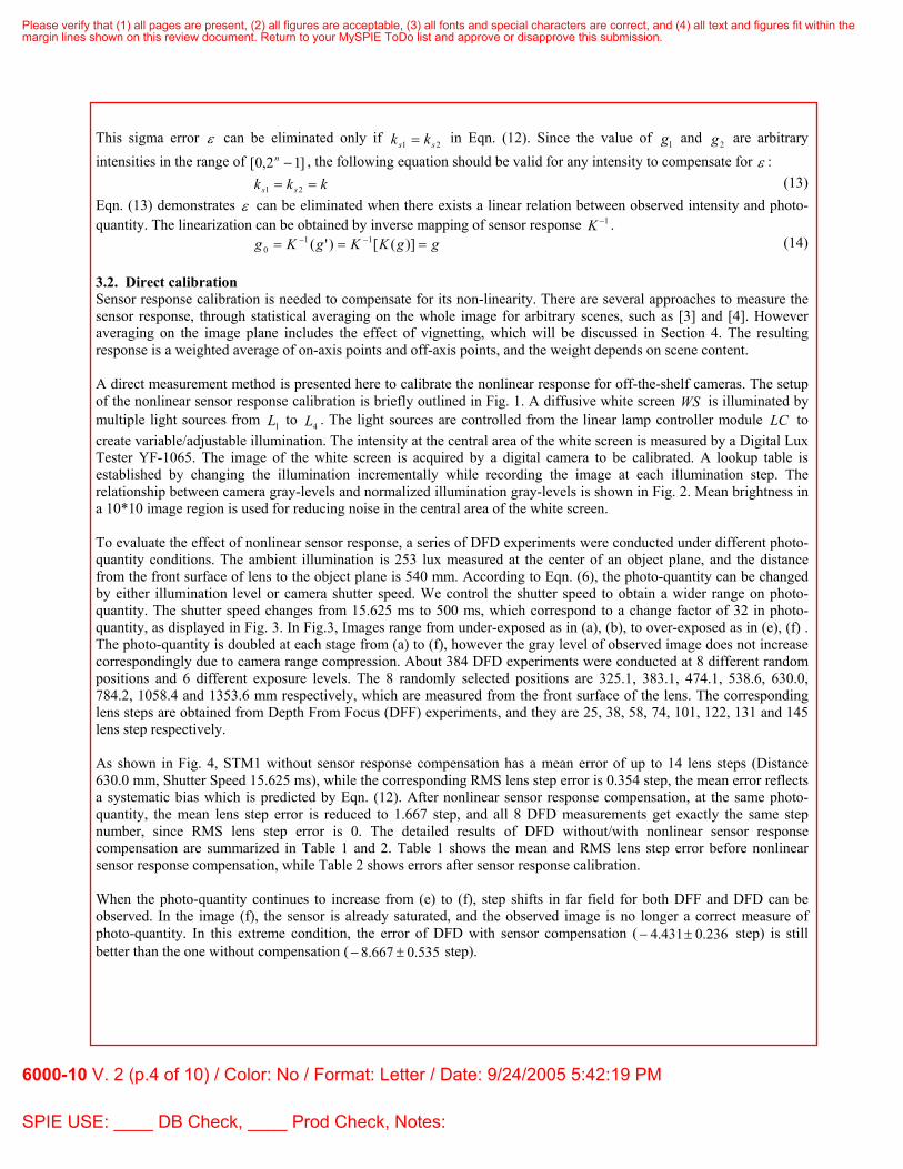
3.2. Direct calibration Sensor response calibration is needed to compensate for its non-linearity. There are several approaches to measure the sensor response, through statistical averaging on the whole image for arbitrary scenes, such as [3] and [4]. However averaging on the image plane includes the effect of vignetting, which will be discussed in Section 4. The resulting response is a weighted average of on-axis points and off-axis points, and the weight depends on scene content. A direct measurement method is presented here to calibrate the nonlinear response for off-the-shelf cameras. The setup of the nonlinear sensor response calibration is briefly outlined in Fig. 1. A diffusive white screen WS is illuminated by multiple light sources from 1L to 4L . The light sources are controlled from the linear lamp controller module LC to create variable/adjustable illumination. The intensity at the central area of the white screen is measured by a Digital Lux Tester YF-1065. The image of the white screen is acquired by a digital camera to be calibrated. A lookup table is established by changing the illumination incrementally while recording the image at each illumination step. The relationship between camera gray-levels and normalized illumination gray-levels is shown in Fig. 2. Mean brightness in a 10*10 image region is used for reducing noise in the central area of the white screen. To evaluate the effect of nonlinear sensor response, a series of DFD experiments were conducted under different photo-quantity conditions. The ambient illumination is 253 lux measured at the center of an object plane, and the distance from the front surface of lens to the object plane is 540 mm. According to Eqn. (6), the photo-quantity can be changed by either illumination level or camera shutter speed. We control the shutter speed to obtain a wider range on photo-quantity. The shutter speed changes from 15.625 ms to 500 ms, which correspond to a change factor of 32 in photo-quantity, as displayed in Fig. 3. In Fig.3, Images range from under-exposed as in (a), (b), to over-exposed as in (e), (f) . The photo-quantity is doubled at each stage from (a) to (f), however the gray level of observed image does not increase correspondingly due to camera range compression. About 384 DFD experiments were conducted at 8 different random positions and 6 different exposure levels. The 8 randomly selected positions are 325.1, 383.1, 474.1, 538.6, 630.0, 784.2, 1058.4 and 1353.6 mm respectively, which are measured from the front surface of the lens. The corresponding lens steps are obtained from Depth From Focus (DFF) experiments, and they are 25, 38, 58, 74, 101, 122, 131 and 145 lens step respectively. As shown in Fig. 4, STM1 without sensor response compensation has a mean error of up to 14 lens steps (Distance 630.0 mm, Shutter Speed 15.625 ms), while the corresponding RMS lens step error is 0.354 step, the mean error reflects a systematic bias which is predicted by Eqn. (12). After nonlinear sensor response compensation, at the same photo-quantity, the mean lens step error is reduced to 1.667 step, and all 8 DFD measurements get exactly the same step number, since RMS lens step error is 0. The detailed results of DFD without/with nonlinear sensor response compensation are summarized in Table 1 and 2. Table 1 shows the mean and RMS lens step error before nonlinear sensor response compensation, while Table 2 shows errors after sensor response calibration. When the photo-quantity continues to increase from (e) to (f), step shifts in far field for both DFF and DFD can be observed. In the image (f), the sensor is already saturated, and the observed image is no longer a correct measure of photo-quantity. In this extreme condition, the error of DFD with sensor compensation ( 236.0431.4 ±− step) is still better than the one without compensation ( 535.0667.8 ±− step).




0 50 100 150 200 250

0

50

100

150

200

250

Normalized Illumination Level

Cam

era

Gra

ylev

el

Figure 1. Setup for nonlinear sensor response

calibration

Figure 2. Nonlinear sensor response

(a) 1x (b) 2x (c) 4x

(d) 8x (e) 16x (f) 32x

Figure 3. Images obtained at different photo-quantity From (a) to (f), images are captured with exposure time of 15.625, 31.25, 62.5, 125, 250 and 500 ms.

Assume the photo-quantity in (a) as a unit measure, the photo-quantity doubles in each stage from (a) to (f)




0 5 10 15 20 25 30 350

25

50

75

100

125

150

Exposure Level [n x]

Ste

ps

woNLwNLDFF

Figure 4. DFD Results without/with nonlinear sensor response calibration woNL: DFD STM1 without Non-Linear sensor response compensation wNL: DFD STM1 with Non-Linear sensor response compensation DFF: Depth From Focus

Exposure 1 Exposure 2 Exposure 3 Exposure 4 Exposure 5 Exposure 6 Mean Std Mean Std Mean Std Mean Std Mean Std Mean Std

Pos 1 6.833 0.000 4.583 0.463 3.083 0.463 0.833 0.000 -0.042 0.354 -1.542 0.518 Pos 2 6.167 0.000 4.917 0.463 3.167 0.000 0.167 0.000 -1.333 0.535 -4.208 0.518 Pos 3 -0.417 0.463 -0.167 0.000 -0.167 0.000 0.333 0.535 0.708 0.354 -2.042 0.354 Pos 4 -7.167 0.000 -6.042 0.354 -3.167 0.000 0.458 0.518 2.333 0.535 1.208 0.518 Pos 5 -14.125 0.354 -12.250 0.707 -6.875 0.641 -0.750 0.463 1.750 0.463 3.250 0.707 Pos 6 -4.625 0.991 -3.750 0.463 -4.125 0.518 -3.250 0.463 -3.250 0.463 -1.500 0.535 Pos 7 -0.583 0.463 -0.583 0.463 -0.708 0.354 0.292 0.354 0.417 0.463 -1.833 0.000 Pos 8 -4.292 0.835 -2.292 0.991 -0.542 1.061 -0.042 0.991 0.458 0.744 -8.667 0.535

Table 1. DFD lens step error by mean and rms

without nonlinear sensor compensation

Exposure 1 Exposure 2 Exposure 3 Exposure 4 Exposure 5 Exposure 6 Mean Std Mean Std Mean Std Mean Std Mean Std Mean Std

Pos 1 -0.347 0.236 -1.139 0.309 0.611 0.000 -0.056 0.000 -0.347 0.236 0.278 0.000 Pos 2 -0.528 0.309 -1.278 0.000 0.056 0.000 -0.153 0.345 -0.278 0.000 -0.861 0.309 Pos 3 -0.139 0.309 0.236 0.236 -0.056 0.000 -0.056 0.000 0.111 0.356 -0.639 0.309 Pos 4 1.194 0.309 2.986 0.236 -0.056 0.000 0.694 0.309 1.528 0.309 -0.181 0.345 Pos 5 1.667 0.000 3.292 0.236 -0.500 0.356 1.250 0.309 1.250 0.309 0.292 0.427 Pos 6 0.083 0.309 0.375 0.345 0.083 0.309 0.167 0.000 -0.125 0.236 -0.958 0.345 Pos 7 -0.611 0.000 -0.569 0.236 -0.611 0.000 -0.319 0.236 -0.611 0.000 -1.611 0.000 Pos 8 -2.472 0.992 -1.306 0.690 -0.514 0.496 -0.347 0.661 -0.556 0.356 -4.431 0.236

Table 2. DFD lens step error by mean and rms

with nonlinear sensor compensation




4 LENS VIGNETTING COMPENSATION

Optical vignetting is the phenomenon wherein the effective light energy transmitted by the optical system decreases with increasing inclination of light rays with respect to the optical axis. The consequence of optical vignetting for a focused scene is merely a reduced brightness towards the image corners. However, optical vignetting can also have a pronounced effect on out-of-focus parts of the image. Because the shape of an Out-Of-Focus Highlight (OOFH) mimics the shape of the clear aperture, this leads to the so-called cat's eye effect. With an increasing distance from the optical axis the shape of the OOFH progressively narrows and starts to resemble a cat's eye. The larger the distance from the image center, the narrower the cat's eye becomes. A vignetting calibration method is used to evaluate the effect of vignetting on DFD measurement. If a uniform illumination is available, the vignetting coefficient could be simply calculated from a single image of a diffusive white screen. However it is difficult to obtain a uniform illumination that is accurate, although not impossible. An alternative way is used in our calibration. The setup for vignetting calibration was similar to that in Fig.1. A 5*5 grid pattern is used as a calibration pattern (see Fig. 3(a) ). In each grid, illumination is measured by the Digital Lux Tester YF-1065 at the center of grids, and the image of the grid pattern is captured by the camera. The gray level obtained is a transformed value of real photo-quantity due to the nonlinearity of sensor response. A lookup table for the reverse mapping discussed in Section 3 is used. The vignetting coefficient is calculated by the ratio of illumination intensity at pixel

),( yx to the intensity at the center of the image. Due to the rotational symmetry property, the relation between vignetting coefficient and pixel distance in polar coordinate is obtained from a third-order polynomial fitting:

1*10*6.7845-*10*3.2488*10*-3.1064)( -52-73-9 ++= ρρρρV (15)

0 50 100 150 200 250 300 350 4000.65

0.7

0.75

0.8

0.85

0.9

0.95

1

Distance [Pixel]

Vig

netti

ng F

acto

r

(a) (b)

Figure 5. Vignetting calibration (a) Pattern (b) Result

The result of vignetting factor vs. pixel distance is shown in Fig. 5(b). From Fig. 5(b), if the DFD AF window is in the center area, the distortion of vignetting can be ignored. (for a 96*96 focusing window, the intensity attenuation is 0.24%). When the focusing window is near a corner of the view, there could be a 12.1% difference in the diagonal direction. In this case, vignetting should be compensated by multiplying the reciprocal of the corresponding vignetting coefficient.




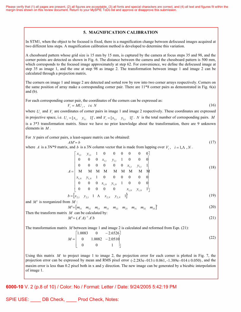
5. MAGNIFICATION CALIBRATION In STM1, when the object to be focused is fixed, there is a magnification change between defocused images acquired at two different lens steps. A magnification calibration method is developed to determine this variation. A chessboard pattern whose grid size is 15 mm by 15 mm, is captured by the camera at focus steps 35 and 98, and the corner points are detected as shown in Fig. 6. The distance between the camera and the chessboard pattern is 500 mm, which corresponds to the focused image approximately at step 62. For convenience, we define the defocused image at step 35 as image 1, and the one at step 98 as image 2. The transformation between image 1 and image 2 can be calculated through a projection matrix. The corners on image 1 and image 2 are detected and sorted row by row into two corner arrays respectively. Corners on the same position of array make a corresponding corner pair. There are 11*8 corner pairs as demonstrated in Fig. 6(a) and (b). For each corresponding corner pair, the coordinates of the corners can be expressed as:

NiMUV ii ∈= , (16) where iU and iV are coordinates of corner pairs in image 1 and image 2 respectively. These coordinates are expressed in projective space, i.e. t

iii yxU ]1[ ,1,1= , and tiii yxV ]1[ ,2,2= . N is the total number of corresponding pairs. M

is a 3*3 transformation matrix. Since we have no prior knowledge about the transformation, there are 9 unknown elements in M . For N pairs of corner pairs, a least-square matrix can be obtained:

bAM =' (17) where A is a 3N*9 matrix, and b is a 3N column vector that is made from lapping over NiVi ,,1, Λ= .

⎥⎥⎥⎥⎥⎥⎥⎥⎥

⎦

⎤

⎢⎢⎢⎢⎢⎢⎢⎢⎢

⎣

⎡

=

10000000010000000001

100000000010000000001

,1,1

,1,1

,1,1

1,11,1

1,11,1

1,11,1

NN

NN

NN

yxyx

yx

yxyx

yx

A ΜΜΜΜΜΜΜΜΜ (18)

[ ]tNN yxyxb 11 ,2,21,21,2 Λ= (19) and 'M is reorganized from M :

[ ]tmmmmmmmmmM 333231232221131211'= (20) Then the transform matrix M can be calculated by:

bAAAM tt 1)(' −= (21) The transformation matrix M between image 1 and image 2 is calculated and reformed from Eqn. (21):

⎥⎥⎥

⎦

⎤

⎢⎢⎢

⎣

⎡−−

=1000510.20082.106526.200083.1

M (22)

Using this matrix M to project image 1 to image 2, the projection error for each corner is plotted in Fig. 7, the projection error can be expressed by mean and RMS pixel error 0.050)014-1.389e- 0.061,013--2.283e( ±± , and the maxim error is less than 0.2 pixel both in x and y direction. The new image can be generated by a bicubic interpolation of image 1.




OdX

dY

Xc (in camera frame)

Yc

(in c

amer

a fra

me)

Extracted corners

100 200 300 400 500 600

50

100

150

200

250

300

350

400

450

OdX

dY

Xc (in camera frame)

Yc

(in c

amer

a fra

me)

Extracted corners

100 200 300 400 500 600

50

100

150

200

250

300

350

400

450

(a)

(b)

Figure 6. Magnification calibration using pattern captured at different steps (a) chessboard pattern captured at step 35 (b) chessboard pattern captured at step 98

-0.2 -0.15 -0.1 -0.05 0 0.05 0.1 0.15 0.2-0.2

-0.15

-0.1

-0.05

0

0.05

0.1

0.15

0.2

X dir [pixel]

Y d

ir [p

ixel

]

Projection Error

Figure 7. Project error from estimated transformation matrix M

6. CONCLUSION

In this paper, calibration methods and procedures for nonlinear sensor response, optical vignetting, and magnification variation are presented. The correctness and effects on the performance of DFD have been evaluated with experiments. These calibrations do not need expensive and strictly controlled laboratory environment. They can be used for off-the-shelf cameras. Therefore, these calibration methods should be of general value to other image based algorithms.




REFERENCES 1. M. Subbarao and G. Surya, "Depth from Defocus: A Spatial Domain Approach", International Journal of

Computer Vision, Vol. 13, No. 3, p. 271-294,1994 2. T. Xian, and M. Subbarao, “Performance Evaluation of Different Depth-From-Defocus (DFD) Techniques”, Proc.

of SPIE, Boston, Oct. 2005 3. S. Mann, “Comparametric Equations with Practical Applications”, IEEE Trans. Image Processing, Vol. 9, No. 8,

P1389-1406, 2000 4. S.Y. Park, and M. Subbarao, “Automatic Focusing of a Digital Still Camera using a Depth-from Defocus

Technique: An Approach for Compensating Non-Linear Camera Response Function”, Internal Technical Report, Computer Vision Lab, ECE, State Univ. of New York at Stony Brook, 2004




Camera Calibration and Perf ormance Evaluation of Depth...

Documents

Transcript of Camera Calibration and Perf ormance Evaluation of Depth...