California State Waters Map Series—Offshore of Scott Creek, California

By Guy R. Cochrane, Peter Dartnell, Samuel Y. Johnson, H. Gary Greene, Mercedes D. Erdey, Bryan E. Dieter, Nadine E. Golden, Charles A. Endris, Stephen R. Hartwell, Rikk G. Kvitek, Clifton W. Davenport, Janet T. Watt, Lisa M. Krigsman, Andrew C. Ritchie, Ray W. Sliter, David P. Finlayson, and Katherine L. Maier

(Guy R. Cochrane and Susan A. Cochran, editors)

Pamphlet to accompany

Open-File Report 2015–1191

2015

U.S. Department of the Interior U.S. Geological Survey

U.S. Department of the Interior SALLY JEWELL, Secretary

U.S. Geological Survey Suzette M. Kimball, Acting Director

U.S. Geological Survey, Reston, Virginia: 2015

For more information on the USGS—the Federal source for science about the Earth, its natural and living resources, natural hazards, and the environment—visit http://www.usgs.gov/ or call 1–888–ASK–USGS (1–888–275–8747).

For an overview of USGS information products, including maps, imagery, and publications, visit http://www.usgs.gov/pubprod/.

To order USGS information products, visit http://store.usgs.gov/.

Any use of trade, firm, or product names is for descriptive purposes only and does not imply endorsement by the U.S. Government.

Although this information product, for the most part, is in the public domain, it also may contain copyrighted materials as noted in the text. Permission to reproduce copyrighted items must be secured from the copyright owner.

Suggested citation: Cochrane, G.R., Dartnell, P., Johnson, S.Y., Greene, H.G., Erdey, M.D., Dieter, B.E., Golden, N.E., Endris, C.A., Hartwell, S.R., Kvitek, R.G., Davenport, C.W., Watt, J.T., Krigsman, L.M., Ritchie, A.C., Sliter, R.W., Finlayson, D.P., and Maier, K.L. (G.R. Cochrane and S.A. Cochran, eds.), 2015, California State Waters Map Series—Offshore of Scott Creek, California: U.S. Geological Survey Open-File Report 2015–1191, pamphlet 40 p., 10 sheets, scale 1:24,000, http://dx.doi.org/10.3133/ofr20151191.

ISSN 2331-1258 (online)

iii

Contents Preface ........................................................................................................................................................................... 1 Chapter 1. Introduction ................................................................................................................................................... 3

By Guy R. Cochrane ................................................................................................................................ 3 Regional Setting ......................................................................................................................................................... 3 Publication Summary .................................................................................................................................................. 5

Chapter 2. Bathymetry and Backscatter-Intensity Maps of the Offshore of Scott Creek Map Area (Sheets 1, 2, and 3) .................................................................................................................................................................................... 8

By Peter Dartnell and Rikk G. Kvitek ........................................................................................................ 8 Chapter 3. Data Integration and Visualization for the Offshore of Scott Creek Map Area (Sheet 4) ............................. 10

By Peter Dartnell .................................................................................................................................... 10 Chapter 4. Seafloor-Character Map of the Offshore of Scott Creek Map Area (Sheet 5) ............................................. 11

By Mercedes D. Erdey and Guy R. Cochrane ........................................................................................ 11 Chapter 5. Ground-Truth Studies for the Offshore of Scott Creek Map Area (Sheet 6) ................................................ 15

By Nadine E. Golden and Guy R. Cochrane .......................................................................................... 15 Chapter 6. Potential Marine Benthic Habitats of the Offshore of Scott Creek Map Area (Sheet 7) .............................. 18

By H. Gary Greene and Charles A. Endris ............................................................................................. 18 Classifying Potential Marine Benthic Habitats .......................................................................................................... 18 Examples of Attribute Coding ................................................................................................................................... 20 Map Area Habitats .................................................................................................................................................... 20

Chapter 7. Subsurface Geology and Structure of the Offshore of Scott Creek Map Area and the Pigeon Point to Southern Monterey Bay Region (Sheets 8 and 9) ........................................................................................................ 21

By Samuel Y. Johnson, Stephen R. Hartwell, Janet T. Watt, and Katherine L. Maier ............................ 21 Data Acquisition ........................................................................................................................................................ 21 Seismic-Reflection Imaging of the Continental Shelf ................................................................................................ 21 Geologic Structure and Recent Deformation ............................................................................................................ 22 Thickness and Depth to Base of Uppermost Pleistocene and Holocene Deposits ................................................... 23

Chapter 8. Geologic and Geomorphic Map of the Offshore of Scott Creek Map Area (Sheet 10) ................................ 27 By Samuel Y. Johnson, Stephen R. Hartwell, and Clifton W. Davenport ............................................... 27

Geologic and Geomorphic Summary ........................................................................................................................ 27 Description of Map Units .......................................................................................................................................... 31

Offshore Geologic And Geomorphic Units ............................................................................................................ 31 Onshore Geologic and Geomorphic Units ............................................................................................................ 31

Acknowledgments ........................................................................................................................................................ 34 References Cited ......................................................................................................................................................... 35

Figures Figure 1–1. Physiography of Pigeon Point to southern Monterey Bay region and its environs .................................... 6 Figure 1–2. Coastal geography of Offshore of Scott Creek map area. ......................................................................... 7 Figure 4–1. Detailed view of ground-truth data, showing accuracy-assessment methodology .................................. 13 Figure 5–1. Photograph of camera sled used in USGS 2007 ground-truth survey..................................................... 15 Figure 5–2. Graph showing distribution of primary and secondary substrate determined from video observations in

Offshore of Scott Creek map area. ......................................................................................................... 17 Figure 8–1. Schematic map showing major offshore structural features northwest of Monterey Bay ........................ 30

iv

Tables Table 4–1. Conversion table showing how video observations of primary substrate, secondary substrate, and

abiotic seafloor complexity are grouped into seafloor-character-map Classes I, II, and III for use in supervised classification and accuracy assessment in Offshore of Scott Creek map area ....................... 14

Table 4–2. Accuracy-assessment statistics for seafloor-character-map classifications in Offshore of Scott Creek map area .................................................................................................................................................. 14

Table 7–1. Area, sediment-thickness, and sediment-volume data for California’s State Waters in Pigeon Point to southern Monterey Bay region (domains 1-6), as well as in Offshore of Scott Creek map area ............... 26

Table 8–1. Areas and relative proportions of offshore geologic map units in Offshore of Scott Creek map area ....... 28

Map Sheets Sheet 1. Colored Shaded-Relief Bathymetry, Offshore of Scott Creek Map Area, California

By Peter Dartnell, Andrew C. Ritchie, David P. Finlayson, and Rikk G. Kvitek Sheet 2. Shaded-Relief Bathymetry, Offshore of Scott Creek Map Area, California

By Peter Dartnell, Andrew C. Ritchie, David P. Finlayson, and Rikk G. Kvitek Sheet 3. Acoustic Backscatter, Offshore of Scott Creek Map Area, California

By Peter Dartnell, Andrew C. Ritchie, David P. Finlayson, and Rikk G. Kvitek Sheet 4. Data Integration and Visualization, Offshore of Scott Creek Map Area, California

By Peter Dartnell Sheet 5. Seafloor Character, Offshore of Scott Creek Map Area, California

By Mercedes D. Erdey and Guy R. Cochrane Sheet 6. Ground-Truth Studies, Offshore of Scott Creek Map Area, California

By Nadine E. Golden, Guy R. Cochrane, and Lisa M. Krigsman Sheet 7. Potential Marine Benthic Habitats, Offshore of Scott Creek Map Area, California

By Charles A. Endris, H. Gary Greene, Bryan E. Dieter, and Mercedes D. Erdey Sheet 8. Seismic-Reflection Profiles, Offshore of Scott Creek Map Area, California

By Samuel Y. Johnson, Stephen R. Hartwell, and Ray W. Sliter Sheet 9. Local (Offshore of Scott Creek Map Area) and Regional (Offshore from Pigeon Point to Southern

Monterey Bay) Shallow-Subsurface Geology and Structure, California By Samuel Y. Johnson, Stephen R. Hartwell, Janet T. Watt, Ray W. Sliter, and Katherine L. Maier

Sheet 10. Offshore and Onshore Geology and Geomorphology, Offshore of Scott Creek Map Area, California By Stephen R. Hartwell, Samuel Y. Johnson, and Clifton W. Davenport

1

California State Waters Map Series—Offshore of Scott Creek, California

By Guy R. Cochrane,1 Peter Dartnell,1 Samuel Y. Johnson,1 H. Gary Greene,2 Mercedes D. Erdey,1 Bryan E. Dieter,2 Nadine E. Golden,1 Charles A. Endris,2 Stephen R. Hartwell,1 Rikk G. Kvitek,3 Clifton W. Davenport,4 Janet T. Watt,1 Lisa M. Krigsman,5 Andrew C. Ritchie,1 Ray W. Sliter,1 David P. Finlayson,1 and Katherine L. Maier1

(Guy R. Cochrane1 and Susan A. Cochran,1 editors)

Preface In 2007, the California Ocean Protection Council initiated the California Seafloor Mapping

Program (CSMP), designed to create a comprehensive seafloor map of high-resolution bathymetry, marine benthic habitats, and geology within California’s State Waters. The program supports a large number of coastal-zone- and ocean-management issues, including the California Marine Life Protection Act (MLPA) (California Department of Fish and Wildlife, 2008), which requires information about the distribution of ecosystems as part of the design and proposal process for the establishment of Marine Protected Areas. A focus of CSMP is to map California’s State Waters with consistent methods at a consistent scale.

The CSMP approach is to create highly detailed seafloor maps through collection, integration, interpretation, and visualization of swath sonar bathymetric data (the undersea equivalent of satellite remote-sensing data in terrestrial mapping), acoustic backscatter, seafloor video, seafloor photography, high-resolution seismic-reflection profiles, and bottom-sediment sampling data. The map products display seafloor morphology and character, identify potential marine benthic habitats, and illustrate both the surficial seafloor geology and shallow subsurface geology. It is emphasized that the more interpretive habitat and geology maps rely on the integration of multiple, new high-resolution datasets and that mapping at small scales would not be possible without such data.

This approach and CSMP planning is based in part on recommendations of the Marine Mapping Planning Workshop (Kvitek and others, 2006), attended by coastal and marine managers and scientists from around the state. That workshop established geographic priorities for a coastal mapping project and identified the need for coverage of “lands” from the shore strand line (defined as Mean Higher High Water; MHHW) out to the 3-nautical-mile (5.6-km) limit of California’s State Waters. Unfortunately, surveying the zone from MHHW out to 10-m water depth is not consistently possible using ship-based surveying methods, owing to sea state (for example, waves, wind, or currents), kelp coverage, and shallow rock outcrops. Accordingly, some of the maps presented in this series commonly do not cover the zone from the shore out to 10-m depth; these “no data” zones appear pale gray on most maps.

This map is part of a series of online U.S. Geological Survey (USGS) publications, each of which includes several map sheets, some explanatory text, and a descriptive pamphlet. Each map sheet

1 U.S. Geological Survey 2 Moss Landing Marine Laboratories, Center for Habitat Studies 3 California State University, Monterey Bay, Seafloor Mapping Lab 4 California Geological Survey 5 National Oceanic and Atmospheric Administration, National Marine Fisheries Service

2

is published as a PDF file. Geographic information system (GIS) files that contain both ESRI6 ArcGIS raster grids (for example, bathymetry, seafloor character) and geotiffs (for example, shaded relief) are also included for each publication. For those who do not own the full suite of ESRI GIS and mapping software, the data can be read using ESRI ArcReader, a free viewer that is available at http://www.esri.com/software/arcgis/arcreader/index.html (last accessed March 5, 2014).

The California Seafloor Mapping Program (CSMP) is a collaborative venture between numerous different federal and state agencies, academia, and the private sector. CSMP partners include the California Coastal Conservancy, the California Ocean Protection Council, the California Department of Fish and Wildlife, the California Geological Survey, California State University at Monterey Bay’s Seafloor Mapping Lab, Moss Landing Marine Laboratories Center for Habitat Studies, Fugro Pelagos, Pacific Gas and Electric Company, National Oceanic and Atmospheric Administration (NOAA, including National Ocean Service – Office of Coast Surveys, National Marine Sanctuaries, and National Marine Fisheries Service), U.S. Army Corps of Engineers, the Bureau of Ocean Energy Management, the National Park Service, and the U.S. Geological Survey.

6 Environmental Systems Research Institute, Inc.

3

Chapter 1. Introduction By Guy R. Cochrane

Regional Setting The map area offshore of the mouth of Scott Creek, in central California, which is referred to

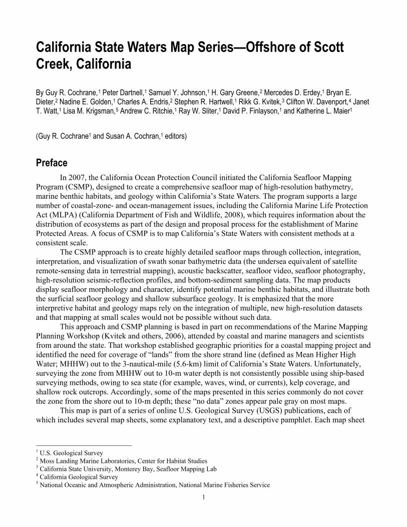
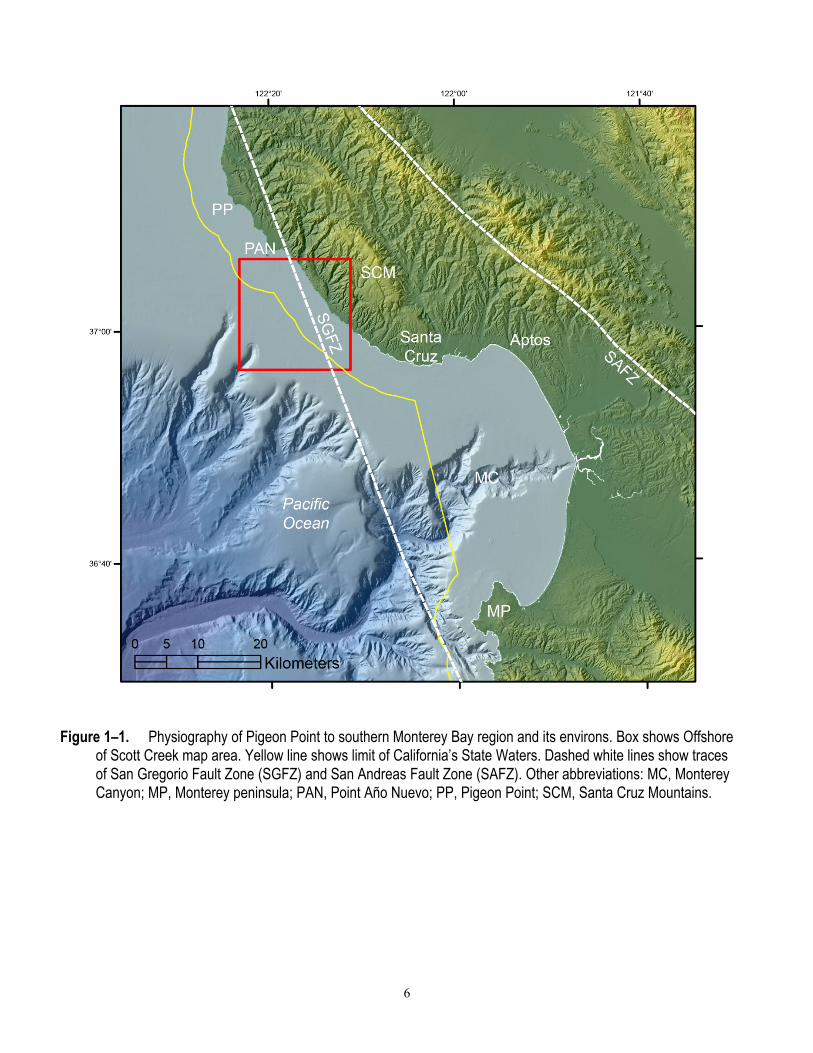
herein as the “Offshore of Scott Creek” map area (figs. 1–1, 1–2), is located on the Pacific Coast, 65 km south of San Francisco and 12 km northwest of Santa Cruz. The onshore part of the Offshore of Scott Creek map area is sparsely populated. The only onshore cultural center is Davenport (fig. 1–2), a small community with a population of less than 500 that lies on the coast near the east edge of the map area. The hilly coastal area is virtually undeveloped, and a large percentage of coastal land in the map area is incorporated in open-space trusts. A lumber mill is on the south flank of Waddell Creek (fig. 1–2), and a large cement plant once operated in Davenport but closed in 2010. Agricultural land (much of which is owned by California Polytechnic State University, San Luis Obispo, and operated partly as a remote campus for agricultural science) is almost entirely limited to coastal areas between the shoreline and the northwest-trending Santa Cruz Mountains (fig. 1–1), on Pleistocene alluvial fan deposits and the lowest emergent marine terrace (see sheet 10). The Santa Cruz Mountains are part of the northwest-trending Coast Ranges that run roughly parallel to the San Andreas Fault Zone (California Geological Survey, 2002).

The map area is cut by an offshore section of the San Gregorio Fault Zone (fig. 1–2), and it lies a few kilometers southwest of the San Andreas Fault Zone (see fig. 1–1; see also, California Geological Survey, 2002). The San Andreas Fault Zone is the most important structure within the Pacific–North American plate boundary, the only continental margin in the world delineated largely by transform faults (Dickinson, 2004). Regional folding and uplift along the coast has been attributed to a westward bend in the San Andreas Fault Zone and also to right-lateral movement along the San Gregorio Fault Zone (Anderson and Menking, 1994). The irregular coastal geomorphology of this area, which consists of low, rocky cliffs and sparse, small pocket beaches backed by low, terraced hills (Griggs and others, 2005), is partly attributable to this ongoing deformation.

The offshore part of the Offshore of Scott Creek map area primarily consists of relatively flat and shallow continental shelf. The shelf dips gently (less than 1°) seaward, so that water depths at the 3-nautical-mile (5.6-km) limit of California’s State Waters range from about 50 to about 65 m. The shelf break, which lies approximately 12 to 20 km from the shoreline, is incised by the heads of several submarine canyons, two of which extend north-northeast well into the outer continental shelf area (see fig. 1–1; see also, lower left corner of fig. 1–2). At water depths of about 130 m, the shelf break approximates the shoreline during the sea-level lowstand of the Last Glacial Maximum (LGM), about 21,000 years ago (see, for example, Stanford and others, 2011).

The shelf in the Offshore of Scott Creek map area is underlain by variable amounts (0 to 25 m) of upper Quaternary shelf, nearshore, and fluvial sediments deposited as sea level fluctuated in the late Pleistocene (see sheet 9). The northernmost part of the map area is characterized by the presence of uplifted bedrock that has been linked to a local transpressional zone in the San Gregorio Fault Zone (Weber, 1990). This uplift, coupled with high wave energy, has resulted in little or no sediment cover in this area where exposures of bedrock are present at water depths of as much as 45 m. The thickest deposits of sediment lie offshore of both Davenport and the mouth of Waddell Creek (see sheet 9).

This part of central California is exposed to large North Pacific swells from the northwest throughout the year. North Pacific swell heights range from 2 to 10 m, the larger swells occurring from October to May (Storlazzi and Wingfield, 2005). During El Niño–Southern Oscillation (ENSO) events, winter storms track farther south than they do in normal (non-ENSO) years, thereby impacting the map

4

area more frequently and with waves of larger heights (Storlazzi and Wingfield, 2005). Bedrock exposed along the coast consists of erosion-resistant sedimentary rocks, and significant erosion events primarily are restricted to storm-wave activity that also erodes the overlying unconsolidated marine-terrace sediments (Griggs and others, 2005).

Coastal sediment transport in the Offshore of Scott Creek map area is characterized by north-to-south littoral transport of sediment that is derived mainly from streams in the Santa Cruz Mountains and also from local coastal erosion (Hapke and others, 2006). Shoreline-change studies indicate long-term erosion; within the region between San Francisco and Davenport, the highest long- and short-term coastal-erosion rates (-1.8 and -2.6 m/y, respectively) occur north of the Offshore of Scott Creek map area, just north of Point Año Nuevo (Hapke and others, 2006) (fig. 1–1). During the last approximately 300 years, as much as 18 million cubic yards (14 million cubic meters) of sand-sized sediment has been eroded from the area between Año Nuevo Island and Point Año Nuevo and transported south (Griggs and others, 2005). Once widened by this pulse of eroded sediment, beaches in the Offshore of Scott Creek map area are now narrowing as the tail end of this mass of sand progresses farther south (Griggs and others, 2005).

Seafloor habitats in the Offshore of Scott Creek map area (see sheet 7 of this report) lie within the Shelf (continental shelf) megahabitat of Greene and others (1999). Significant rocky outcrops, which support kelp-forest communities in the nearshore and rocky-reef communities in deeper water, dominate the inner shelf waters. Sand-filled paleochannels cut through the rocky reefs offshore of coastal creeks. In the midshelf to outer shelf areas, habitats grade seaward from sand to fine-grained sand and mud. Offshore of Davenport, an extensive area of depressions, which are caused by current scour, extends out to 50 m water depth (see sheet 3).

Benthic species observed in the Offshore of Scott Creek map area are natives of the cold-temperate biogeographic zone that is called either the “Oregonian province” (Briggs, 1974) or the “northern California ecoregion” (Spalding and others, 2007). This biogeographic province is maintained by the long-term stability of the southward-flowing California Current, the eastern limb of the North Pacific subtropical gyre that flows from southern British Columbia to Baja California. At its midpoint off central California, the California Current transports subarctic surface (0–500 m deep) waters southward, about 150 to 1,300 km from shore (Lynn and Simpson, 1987; Collins and others, 2000). Seasonal northwesterly winds (Inman and Jenkins, 1999) that are, in part, responsible for the California Current, generate coastal upwelling. The south end of the Oregonian province is at Point Conception (about 320 km south of the map area), although its associated phylogeographic group of marine fauna may extend beyond to the area offshore of Los Angeles in southern California (Dawson and others, 2006). The ocean off of central California has experienced a warming over the last 50 years that is driving an ecosystem shift away from the productive subarctic regime towards a depopulated subtropical environment (McGowan and others, 1998).

Biological productivity resulting from coastal upwelling supports populations of Sooty Shearwater (Puffinus griseus), Western Gull (Larus occidentalis), Common Murre (Uria aalge), Cassin’s Auklet (Ptychoramphus aleuticus), and many other less populous bird species (Ainley and Hyrenbach, 2010). In addition, an observable recovery of Humpback and Blue Whales (Megaptera novaeangliae and Balaenoptera musculus, respectively) has occurred in the area; both species are dependent on coastal upwelling to provide nutrients (Calambokidis and Barlow, 2004). The large extent of exposed inner shelf bedrock supports large forests of “bull kelp” (Nereocystis luetkeana) (Miller and Estes, 1989), which is well adapted for high-wave-energy environments (Koehl and Wainwright, 1977). The kelp beds are the northernmost known habitat for the population of southern sea otters (Enhydra lutris nereis) (Tinker and others, 2008). Common fish species found in the kelp beds and rocky reefs include blue rockfish (Sebastes mystinus), black rockfish (Sebastes melanops), olive rockfish (Sebastes serranoides), kelp rockfish (Sebastes atrovirens), gopher rockfish (Sebastes carnatus), black-and-yellow

5

rockfish (Sebastes chrysomelas), painted greenling (Oxylebius pictus), kelp greenling (Hexagrammos decagrammus), and lingcod (Ophiodon elongatus) (Stephens and others, 2006).

Publication Summary This publication about the Offshore of Scott Creek map area includes ten map sheets that contain

explanatory text, in addition to this descriptive pamphlet and a data catalog of geographic information system (GIS) files. Sheets 1, 2, and 3 combine data from four different sonar surveys to generate comprehensive high-resolution bathymetry and acoustic-backscatter coverage of the map area. These data reveal a range of physiographic features (highlighted in the perspective views on sheet 4) such as the flat, sediment-covered, inner continental to midcontinental shelf, as well as shallow “scour depressions” and local, tectonically controlled bedrock uplifts. To validate geological and biological interpretations of the sonar data shown in sheets 1, 2, and 3, the U.S. Geological Survey towed a camera sled over specific offshore locations, collecting both video and photographic imagery; these “ground-truth” surveying data are summarized on sheet 6. Sheet 5 is a “seafloor character” map, which classifies the seafloor on the basis of depth, slope, rugosity (ruggedness), and backscatter intensity and which is further informed by the ground-truth-survey imagery. Sheet 7 is a map of “potential habitats,” which are delineated on the basis of substrate type, geomorphology, seafloor process, or other attributes that may provide a habitat for a specific species or assemblage of organisms. Sheet 8 compiles representative seismic-reflection profiles from the map area, providing information on the subsurface stratigraphy and structure of the map area. Sheet 9 shows the distribution and thickness of young sediment (deposited over the last about 21,000 years, during the most recent sea-level rise) in both the map area and the larger Pigeon Point to southern Monterey Bay region, interpreted on the basis of the seismic-reflection data. Sheet 10 is a geologic map that merges onshore geologic mapping (compiled from existing maps by the California Geological Survey) and new offshore geologic mapping that is based on integration of high-resolution bathymetry and backscatter imagery (sheets 1, 2, 3), seafloor-sediment and rock samples (Reid and others, 2006), digital camera and video imagery (sheet 6), and high-resolution seismic-reflection profiles (sheet 8).

The information provided by the map sheets, pamphlet, and data catalog has a broad range of applications. High-resolution bathymetry, acoustic backscatter, ground-truth-surveying imagery, and habitat mapping all contribute to habitat characterization and ecosystem-based management by providing essential data for delineation of marine protected areas and ecosystem restoration. Many of the maps provide high-resolution baselines that will be critical for monitoring environmental change associated with climate change, coastal development, or other forcings. High-resolution bathymetry is a critical component for modeling coastal flooding caused by storms and tsunamis, as well as inundation associated with longer term sea-level rise. Seismic-reflection and bathymetric data help characterize earthquake and tsunami sources, critical for natural-hazard assessments of coastal zones. Information on sediment distribution and thickness is essential to the understanding of local and regional sediment transport, as well as the development of regional sediment-management plans. In addition, siting of any new offshore infrastructure (for example, pipelines, cables, or renewable-energy facilities) will depend on high-resolution mapping. Finally, this mapping will both stimulate and enable new scientific research and also raise public awareness of, and education about, coastal environments and issues.

6

Figure 1–1. Physiography of Pigeon Point to southern Monterey Bay region and its environs. Box shows Offshore of Scott Creek map area. Yellow line shows limit of California’s State Waters. Dashed white lines show traces of San Gregorio Fault Zone (SGFZ) and San Andreas Fault Zone (SAFZ). Other abbreviations: MC, Monterey Canyon; MP, Monterey peninsula; PAN, Point Año Nuevo; PP, Pigeon Point; SCM, Santa Cruz Mountains.

7

Figure 1–2. Coastal geography of Offshore of Scott Creek map area. Yellow line shows limit of California’s State Waters. Dashed white line shows trace of San Gregorio Fault Zone (SGFZ). Other abbreviations: AP, Agua Puera Creek; SC, Scott Creek; SV, San Vincente Creek; WC, Waddell Creek.

8

Chapter 2. Bathymetry and Backscatter-Intensity Maps of the Offshore of Scott Creek Map Area (Sheets 1, 2, and 3) By Peter Dartnell and Rikk G. Kvitek

The colored shaded-relief bathymetry (sheet 1), the shaded-relief bathymetry (sheet 2), and the acoustic-backscatter (sheet 3) maps of the Offshore of Scott Creek map area in central California were generated from bathymetry and backscatter data collected by Fugro Pelagos, by California State University, Monterey Bay (CSUMB), and by the U.S. Geological Survey (USGS) (fig. 1 on sheets 1, 2, 3). Mapping was completed between 2006 and 2009, using a combination of 400-kHz Reson 7125 and 244-kHz Reson 8101 multibeam echosounders, as well as a 234-kHz SWATHplus bathymetric sidescan-sonar system. These mapping missions combined to collect both bathymetry (sheets 1, 2) and acoustic-backscatter data (sheet 3) from about the 10-m isobath to beyond the 3-nautical-mile limit of California’s State Waters.

During the Fugro Pelagos and CSUMB mapping missions, an Applanix POS MV (Position and Orientation System for Marine Vessels) was used to accurately position the vessels during data collection, and it also accounted for vessel motion such as heave, pitch, and roll (position accuracy, ±2 m; pitch, roll, and heading accuracy, ±0.02°; heave accuracy, ±5%, or 5 cm). To account for tidal-cycle fluctuations, Fugro Pelagos used StarFix HP and XP real-time kinematic (RTK) GPS receivers, and CSUMB used a NavCom 2050 receiver; in addition, sound-velocity profiles were collected with an Applied Microsystems (AM) SVPlus sound velocimeter. Soundings were corrected for vessel motion using the Applanix POS MV data, for variations in water-column sound velocity using the AM SVPlus data, and for variations in water height (tides) using vertical-position data from the RTK receivers. The backscatter data were postprocessed using Geocoder, within which the backscatter intensities were radiometrically corrected (including despeckling and angle-varying gain adjustments), and the position of each acoustic sample was geometrically corrected for slant range on a line-by-line basis. After the lines were corrected, they were mosaicked into 1- or 2-m-resolution images. Overlap between parallel lines was resolved using a priority table whose values were based on the distance of each sample from the ship track, with the samples that were closest to and furthest from the ship track being given the lowest priority. An anti-aliasing algorithm was also applied. The mosaics were then exported as georeferenced TIFF images, imported into a geographic information system (GIS), and converted to GRIDs at 2-m resolution.

During the USGS mapping mission, GPS data with real-time-kinematic corrections were combined with measurements of vessel motion (heave, pitch, and roll) in a CodaOctopus F180 attitude-and-position system to produce a high-precision vessel-attitude packet. This packet was transmitted to the acquisition software in real time and combined with instantaneous sound-velocity measurements at the transducer head before each ping. The returned samples were projected to the seafloor using a ray-tracing algorithm that works with previously measured sound-velocity profiles. Statistical filters were applied to discriminate seafloor returns (soundings) from unintended targets in the water column (Ritchie and others, 2010). The backscatter data were postprocessed using USGS software (D.P. Finlayson, written commun., 2011) that normalizes for time-varying signal loss and beam-directivity differences. Thus, the raw 16-bit backscatter data were gain-normalized to enhance the backscatter of the SWATHplus system. The resulting normalized-amplitude values were rescaled to 16-bit and gridded into GeoJPEGs using GRID Processor Software, then imported into a GIS and converted to GRIDs.

Processed soundings from the different mapping missions were exported from the acquisition or processing software as XYZ files and bathymetric surfaces. All of the surfaces were then merged into one overall 2-m-resolution bathymetric-surface model and clipped to the boundary of the map area.

9

Difference calculations of the overlapping bathymetry grids showed that there is good agreement (a mean difference of only a 0.18 m, with 0.34 m standard deviation) between the 2006–2007 Fugro Pelagos and CSUMB bathymetry data and the overlapping 2009 USGS data, even though the data were collected at different times using different mapping systems.

An illumination having an azimuth of 300° and from 45° above the horizon was then applied to the bathymetric surface to create the shaded-relief imagery (sheets 1, 2). In addition, a modified “rainbow” color ramp was applied to the bathymetry data for sheet 1, using reds to represent shallower depths, and yellows to represent greater depths (note that the Offshore of Scott Creek map area requires only the shallower part of the full-rainbow color ramp used on some of the other maps in the California State Waters Map Series; see, for example, Kvitek and others, 2012). This colored bathymetry surface was draped over the shaded-relief imagery at 60-percent transparency to create a colored shaded-relief map (sheet 1). Note that the ripple patterns and parallel lines that are apparent within the map area are data-collection and -processing artifacts. In addition, lines at the borders of some surveys are the result of slight differences in depth, as measured by different mapping systems in different years. These various artifacts are made obvious by the hillshading process.

Bathymetric contours (sheets 1, 2, 3, 5, 7, 10) were generated at 10-m intervals from the merged 2-m-resolution bathymetric surface. The merged surface was smoothed using the Focal Mean tool in ArcGIS and a circular neighborhood that has a radius of between 20 and 30 m (depending on the location). The contours were generated from this smoothed surface using the Spatial Analyst Contour tool in ArcGIS. The most continuous contour segments were preserved; smaller segments and isolated island polygons were excluded from the final output. The contours were then clipped to the boundary of the map area.

The acoustic-backscatter imagery from each mapping system and processing method were merged into their own individual grids. These individual grids, which cover different areas, were displayed in a GIS to create a composite acoustic-backscatter map (sheet 3). On the map, brighter tones indicate higher backscatter intensity, and darker tones indicate lower backscatter intensity. The intensity represents a complex interaction between the acoustic pulse and the seafloor, as well as characteristics within the shallow subsurface, providing a general indication of seafloor texture and composition. Backscatter intensity depends on the acoustic source level; the frequency used to image the seafloor; the grazing angle; the composition and character of the seafloor, including grain size, water content, bulk density, and seafloor roughness; and some biological cover. Harder and rougher bottom types such as rocky outcrops or coarse sediment typically return stronger intensities (high backscatter, lighter tones), whereas softer bottom types such as fine sediment return weaker intensities (low backscatter, darker tones). The differences in backscatter intensity that are apparent in some areas of the map on sheet 3 are due to the different frequencies of the mapping systems, as well as to different processing techniques. Parallel lines of higher backscatter intensity throughout the map area are data-collection and -processing artifacts.

The onshore-area image was generated by applying an illumination having an azimuth of 300° and from 45° above the horizon to 2-m-resolution topographic-lidar data from the California Coastal Conservancy (available from National Oceanic and Atmospheric Administration [NOAA] Coastal Service Center’s Digital Coast at http://www.csc.noaa.gov/digitalcoast/data/coastallidar/) and to 10-m-resolution topographic-lidar data from the U.S. Geological Survey’s National Elevation Dataset (available at http://ned.usgs.gov/).

10

Chapter 3. Data Integration and Visualization for the Offshore of Scott Creek Map Area (Sheet 4) By Peter Dartnell

Mapping California’s State Waters has produced a vast amount of acoustic and visual data, including bathymetry, acoustic backscatter, seismic-reflection profiles, and seafloor video and photography. These data are used by researchers to develop maps, reports, and other tools to assist in the coastal and marine spatial-planning capability of coastal-zone managers and other stakeholders. For example, seafloor-character (sheet 5), habitat (sheet 7), and geologic (sheet 10) maps of the Offshore of Scott Creek map area may assist in the designation of Marine Protected Areas, as well as in their monitoring. These maps and reports also help to analyze environmental change owing to sea-level rise and coastal development, to model and predict sediment and contaminant budgets and transport, to site offshore infrastructure, and to assess tsunami and earthquake hazards. To facilitate this increased understanding and to assist in product development, it is helpful to integrate the different datasets and then view the results in three-dimensional representations such as those displayed on the data integration and visualization sheet for the Offshore of Scott Creek map area (sheet 4).

The maps and three-dimensional views on sheet 4 were created using a series of geographic information systems (GIS) and visualization techniques. Using GIS, the bathymetric and topographic data (sheet 1) were converted to ASCIIRASTER format files, and the acoustic-backscatter data (sheet 3) were converted to geoTIFF images. The bathymetric and topographic data were imported in the Fledermaus® software (QPS). The bathymetry was color-coded to closely match the colored shaded-relief bathymetry on sheet 1, in which reds represent shallower depths and yellows represent deeper depths; topographic data were shown in gray shades. Acoustic-backscatter geoTIFF images also were draped over the bathymetry data. The colored bathymetry, topography, and draped backscatter were then tilted and panned to create the perspective views such as those shown in figures 1, 2, 4, 5, and 6 on sheet 4. These views highlight the seafloor morphology in the Offshore of Scott Creek map area, which includes an extensive, featureless, sedimented seafloor, as well as layered, folded, and fractured bedrock.

Video-mosaic images created from digital seafloor video (for example, fig. 3 on sheet 4) display the geologic complexity (rock, sand, and mud; see sheet 10) and biologic complexity of the seafloor. Whereas photographs capture high-quality snapshots of smaller areas of the seafloor (see sheet 6), video mosaics capture larger areas and can show transition zones between seafloor environments. Digital seafloor video is collected from a camera sled towed approximately 1 to 2 meters above the seafloor, at speeds less than 1 nautical mile/hour. Using standard video-editing software, as well as software developed at the Center for Coastal and Ocean Mapping, University of New Hampshire, the digital video is converted to AVI format, cut into 1- to 2-minute sections, and desampled to every second or third frame. The frames are merged together using pattern-recognition algorithms from one frame to the next and converted to a TIFF image. The images are then rectified to the bathymetry data using ship navigation recorded with the video and layback estimates of the towed camera sled.

Block diagrams that combine the bathymetry with seismic-reflection-profile data help integrate surface and subsurface observations, especially stratigraphic and structural relations (for example, fig. 6 on sheet 4). These block diagrams were created by converting digital seismic-reflection-profile data (see sheet 8) into TIFF images, while taking note of the starting and ending coordinates and maximum and minimum depths. The images were then imported into the Fledermaus® software as vertical images and merged with the bathymetry imagery.

11

Chapter 4. Seafloor-Character Map of the Offshore of Scott Creek Map Area (Sheet 5) By Mercedes D. Erdey and Guy R. Cochrane

The California State Marine Life Protection Act (MLPA) calls for protecting representative types of habitat in different depth zones and environmental conditions. A science team, assembled under the auspices of the California Department of Fish and Wildlife (CDFW), has identified seven substrate-defined seafloor habitats in California’s State Waters that can be classified using sonar data and seafloor video and photography. These habitats include rocky banks, intertidal zones, sandy or soft ocean bottoms, underwater pinnacles, kelp forests, submarine canyons, and seagrass beds. The following five depth zones, which determine changes in species composition, have been identified: Depth Zone 1, intertidal; Depth Zone 2, intertidal to 30 m; Depth Zone 3, 30 to 100 m; Depth Zone 4, 100 to 200 m; and Depth Zone 5, deeper than 200 m (California Department of Fish and Wildlife, 2008). The CDFW habitats, with the exception of depth zones, can be considered a subset of a broader classification scheme of Greene and others (1999) that has been used by the U.S. Geological Survey (USGS) (Cochrane and others, 2003, 2005). These seafloor-character maps are generalized polygon shapefiles that have attributes derived from Greene and others (2007).

A 2007 Coastal Map Development Workshop, hosted by the USGS in Menlo Park, California, identified the need for more detailed (relative to Greene and others’ [1999] attributes) raster products that preserve some of the transitional character of the seafloor when substrates are mixed and (or) they change gradationally. The seafloor-character map, which delineates a subset of the CDFW habitats, is a GIS-derived raster product that can be produced in a consistent manner from data of variable quality covering large geographic regions.

The following four substrate classes are identified in the Offshore of Scott Creek map area: • Class I: Fine- to medium-grained smooth sediment • Class II: Mixed smooth sediment and rock • Class III: Rock and boulder, rugose • Class IV: Medium- to coarse-grained sediment (in scour depressions) The seafloor-character map of the Offshore of Scott Creek map area (sheet 5) was produced

using video-supervised maximum-likelihood classification of the bathymetry and intensity of return from sonar systems, following the method described by Cochrane (2008). The two variants used in this classification were backscatter intensity and derivative rugosity. The rugosity calculation was performed using the Terrain Ruggedness (VRM) tool within the Benthic Terrain Modeler toolset v. 3.0 (Wright and others, 2012; available at http://esriurl.com/5754).

Classes I, II, and III values were delineated using multivariate analysis. Class IV (medium- to coarse-grained sediment, in scour depressions) values were determined on the basis of their visual characteristics using both shaded-relief bathymetry and backscatter (slight depression in the seafloor, very high backscatter return). The resulting map (gridded at 2 m) was cleaned by hand to remove data-collection artifacts (for example, the trackline nadir).

On the seafloor-character map (sheet 5), the four substrate classes have been colored to indicate the California MLPA depth zones and the Coastal and Marine Ecological Classification Standard (CMECS) slope zones (Madden and others, 2008) in which they belong. The California MLPA depth zones are Depth Zone 1 (intertidal), Depth Zone 2 (intertidal to 30 m), Depth Zone 3 (30 to 100 m), Depth Zone 4 (100 to 200 m), and Depth Zone 5 (greater than 200 m); in the Offshore of Scott Creek map area, only Depth Zones 2 and 3 are present. The slope classes that represent the CMECS slope

12

zones are Slope Class 1 = flat (0° to 5°), Slope Class 2 = sloping (5° to 30°), Slope Class 3 = steeply sloping (30° to 60°), Slope Class 4 = vertical (60° to 90°), and Slope Class 5 = overhang (greater than 90°); in the Offshore of Scott Creek map area, only Slope Classes 1 and 2 are present. The final classified seafloor-character raster map image has been draped over the shaded-relief bathymetry for the area (sheets 1 and 2) to produce the image shown on the seafloor-character map on sheet 5.

The seafloor-character classification also is summarized on sheet 5 in table 1. Fine- to medium-grained smooth sediment (sand and mud) makes up 80.6 percent (103.2 km2) of the map area: 9.1 percent (11.7 km2) is in Depth Zone 2, and 71.5 percent (91.5 km2) is in Depth Zone 3. Mixed smooth sediment (sand and gravel) and rock (that is, sediment typically forming a veneer over bedrock, or rock outcrops having little to no relief) make up 8.1 percent (10.3 km2) of the map area: 2.7 percent (3.5 km2) is in Depth Zone 2, and 5.4 percent (6.8 km2) is in Depth Zone 3. Rock and boulder, rugose (rock and boulder outcrops having high surficial complexity) makes up 10.4 percent (13.3 km2) of the map area: 7.4 percent (9.4 km2) is in Depth Zone 2, and 3.0 percent (3.9 km2) is in Depth Zone 3. Medium- to coarse-grained sediment (in scour depressions consisting of material that is coarser than the surrounding seafloor) makes up 0.9 percent (1.2 km2) of the map area: 0.1 percent (0.1 km2) is in Depth Zone 2, and 0.8 percent (1.1 km2) is in Depth Zone 3.

A small number of video observations were used to supervise the numerical classification of the seafloor. All video observations (see sheet 6) are used for accuracy assessment of the seafloor-character map after classification. To compare observations to classified pixels, each observation point is assigned a class (I, II, or III), according to the visually derived, major or minor geologic component (for example, sand or rock) and the abiotic complexity (vertical variability) of the substrate recorded during ground-truth surveys (table 4–1; see, also, chapter 5 of this pamphlet). Class IV values were assigned on the basis of the observation of one or more of a group of features that includes both larger scale bedforms (for example, sand waves), as well as sediment-filled scour depressions that resemble the “rippled scour depressions” of Cacchione and others (1984) and Phillips and others (2007) and also the “sorted bedforms” of Murray and Thieler (2004), Goff and others (2005), and Trembanis and Hume (2011). On the geologic map (see sheet 10 of this report), they are referred to as “marine shelf scour depressions.”

Next, circular buffer areas were created around individual observation points using a 10-m radius to account for layback and positional inaccuracies inherent to the towed-camera system. The radius length is an average of the distances between the positions of sharp interfaces seen on both the video (the position of the ship at the time of observation) and sonar data, plus the distance covered during a 10-second observation period at an average speed of 1 nautical mile/hour. Each buffer, which covers more than 300 m2, contains approximately 77 pixels. The classified (I, II, III) buffer is used as a mask to extract pixels from the seafloor-character map. These pixels are then compared to the class of the buffer. For example, if the shipboard-video observation is Class II (mixed smooth sediment and rock), but 12 of the 77 pixels within the buffer area are characterized as Class I (fine- to medium-grained smooth sediment), and 15 (of the 77) are characterized as Class III (rock and boulder, rugose), then the comparison would be “Class I, 12; Class II, 50; Class III, 15” (fig. 4–1). If the video observation of substrate is Class II, then the classification is accurate because the majority of seafloor pixels in the buffer are Class II. The accuracy values in table 4–2 represent the final of several classification iterations aimed at achieving the best accuracy, given the variable quality of sonar data (see discussion in Cochrane, 2008) and the limited ground-truth information available when compared to the continuous coverage provided by swath sonar. Presence/absence values in table 4–2 reflect the percentages of observations where the sediment classification of at least one pixel within the buffer zone agreed with the observed sediment type at a certain location.

The seafloor in the Offshore of Scott Creek map area is covered predominantly by Class I sediment composed of soft, unconsolidated sand and mud. Several exposures of the deformed and differentially eroded rocks of the Santa Cruz Mudstone (Class III) are present in the nearshore area

13

offshore of Scott Creek and Davenport. The northern part of the map area is dominated by exposures of the Monterey and Purisima Formations offshore of Point Año Nuevo. The bedrock outcrops are covered with varying thicknesses of fine (Class I) to coarse (Class II) sediment. Several areas of medium- to coarse-grained scour depressions (Class IV) also have been identified, most commonly adjacent to rock outcrops, and they reach water depths of about 55 m.

The classification accuracy of Classes I, III, and IV (73 percent, 67 percent, and 92 percent accurate, respectively; table 4–2) is determined by comparing the shipboard video observations and the classified map. The weaker (33 percent accurate) agreement in Class II (mixed smooth sediment and rock and flat rock outcrop) likely is due to the relatively narrow and intermittent nature of transition zones from sediment to rock and also the size of the buffer. The bedrock outcrops in this area are composed of differentially eroded sedimentary rocks (Cochrane and Lafferty, 2002). Erosion of softer layers produces Class I and II sediments, resulting in patchy areas of rugose rock and boulder habitat (Class III) on the seafloor. A single buffered observation locale of 78 pixels, therefore, is likely to be interspersed with other classes of pixels, in addition to Class III. Percentages for presence/absence within a buffer also were calculated as a better measure of the accuracy of the classification for patchy rock habitat. The presence/absence accuracy was found to be significant for all classes (90 percent for Class I, 64 percent for Class II, 95 percent for Class III, and 100 percent for Class IV).

Figure 4–1. Detailed view of ground-truth data, showing accuracy-assessment methodology. A, Dots illustrate ground-truth observation points, each of which represents 10-second window of substrate observation plotted over seafloor-character grid; circle around dot illustrates area of buffer depicted in B. B, Pixels of seafloor-character data within 10-m-radius buffer centered on one individual ground-truth video observation.

14

Table 4–1. Conversion table showing how video observations of primary substrate (more than 50 percent seafloor coverage), secondary substrate (more than 20 percent seafloor coverage), and abiotic seafloor complexity (in first three columns) are grouped into seafloor-character-map Classes I, II, and III for use in supervised classification and accuracy assessment in Offshore of Scott Creek map area.

[In areas of low visibility where primary and secondary substrate could not be identified with confidence, recorded observations of substrate (in fourth column) were used to assess accuracy]

Primary-substrate component Secondary-substrate component Abiotic seafloor complexity Low-visibility observations

Class I mud sand low

sand mud low

sand mud trace

sand sand low

sediment

ripples

Class II cobbles sand low

rock mud low

rock sand low

rock rock low

boulders sand moderate

sand cobbles low

sand rock low

sand rock moderate

Class III boulders cobbles moderate

boulders rock moderate

cobbles boulders moderate

rock boulders high

rock boulders moderate

rock cobbles moderate

rock rock high

rock rock moderate

rock sand high

rock sand moderate

Table 4–2. Accuracy-assessment statistics for seafloor-character-map classifications in Offshore of Scott Creek map area.

[Accuracy assessments are based on video observations]

Class Number of observations % majority % presence/absence

I—Fine- to medium-grained smooth sediment 190 72.6 90.0 II—Mixed smooth sediment and rock 38 32.9 64.4 III—Rock and boulder, rugose 168 66.9 94.9 IV—Medium- to coarse-grained sediment (in scour depressions) 31 91.9 100.0

15

Chapter 5. Ground-Truth Studies for the Offshore of Scott Creek Map Area (Sheet 6) By Nadine E. Golden and Guy R. Cochrane

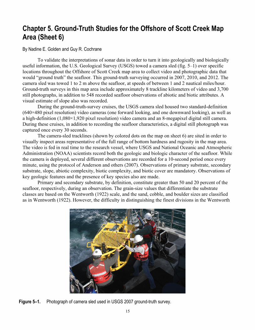
To validate the interpretations of sonar data in order to turn it into geologically and biologically useful information, the U.S. Geological Survey (USGS) towed a camera sled (fig. 5–1) over specific locations throughout the Offshore of Scott Creek map area to collect video and photographic data that would “ground truth” the seafloor. This ground-truth surveying occurred in 2007, 2010, and 2012. The camera sled was towed 1 to 2 m above the seafloor, at speeds of between 1 and 2 nautical miles/hour. Ground-truth surveys in this map area include approximately 8 trackline kilometers of video and 3,700 still photographs, in addition to 548 recorded seafloor observations of abiotic and biotic attributes. A visual estimate of slope also was recorded.

During the ground-truth-survey cruises, the USGS camera sled housed two standard-definition (640×480 pixel resolution) video cameras (one forward looking, and one downward looking), as well as a high-definition (1,080×1,920 pixel resolution) video camera and an 8-megapixel digital still camera. During these cruises, in addition to recording the seafloor characteristics, a digital still photograph was captured once every 30 seconds.

The camera-sled tracklines (shown by colored dots on the map on sheet 6) are sited in order to visually inspect areas representative of the full range of bottom hardness and rugosity in the map area. The video is fed in real time to the research vessel, where USGS and National Oceanic and Atmospheric Administration (NOAA) scientists record both the geologic and biologic character of the seafloor. While the camera is deployed, several different observations are recorded for a 10-second period once every minute, using the protocol of Anderson and others (2007). Observations of primary substrate, secondary substrate, slope, abiotic complexity, biotic complexity, and biotic cover are mandatory. Observations of key geologic features and the presence of key species also are made.

Primary and secondary substrate, by definition, constitute greater than 50 and 20 percent of the seafloor, respectively, during an observation. The grain-size values that differentiate the substrate classes are based on the Wentworth (1922) scale, and the sand, cobble, and boulder sizes are classified as in Wentworth (1922). However, the difficulty in distinguishing the finest divisions in the Wentworth

Figure 5–1. Photograph of camera sled used in USGS 2007 ground-truth survey.

16

(1922) scale during video observations made it necessary to aggregate some grain-size classes, as was done in the Anderson and others (2007) methodology: the granule and pebble sizes have been grouped together into a class called “gravel,” and the clay and silt sizes have been grouped together into a class called “mud.” In addition, hard bottom and clasts larger than boulder size are classified as “rock.” Benthic-habitat complexity, which is divided into abiotic (geologic) and biotic (biologic) components, refers to the visual classification of local geologic features and biota that potentially can provide refuge for both juvenile and adult forms of various species (Tissot and others, 2006).

Sheet 6 contains a smaller, simplified (depth-zone symbology has been removed) version of the seafloor-character map on sheet 5. On this simplified map, the camera-sled tracklines used to ground-truth-survey the sonar data are shown by aligned colored dots, each dot representing the location of a recorded observation. A combination of abiotic attributes (primary- and secondary-substrate compositions), as well as vertical variability, were used to derive the different classes represented on the seafloor-character map (sheet 5); on the simplified map, the derived classes are represented by colored dots. Also on this map are locations of the detailed views of seafloor character, shown by boxes (Boxes A through E); for each view, the box shows the locations (indicated by colored stars) of representative seafloor photographs. For each photograph, an explanation of the observed seafloor characteristics recorded by USGS and NOAA scientists is given. Note that individual photographs often show more substrate types than are reported as the primary and secondary substrate. Organisms, when present, are labeled on the photographs.

The ground-truth survey is designed to investigate areas that represent the full spectrum of high-resolution multibeam bathymetry and backscatter-intensity variation. Figure 5–2 shows that the seafloor surface in the Offshore of Scott Creek map area predominantly consists of high-relief rocky habitat in the nearshore and also out to water depths of 45 m; sand and mud habitat dominates in deeper waters (see also, sheets 5, 7, 9).

17

Figure 5–2. Graph showing distribution of primary and secondary substrate determined from video observations in Offshore of Scott Creek map area.

18

Chapter 6. Potential Marine Benthic Habitats of the Offshore of Scott Creek Map Area (Sheet 7) By H. Gary Greene and Charles A. Endris

The map on sheet 7 shows “potential” marine benthic habitats in the Offshore of Scott Creek map area, representing a substrate type, geomorphology, seafloor process, or any other attribute that may provide a habitat for a specific species or assemblage of organisms. This map, which is based largely on seafloor geology, also integrates information displayed on several other thematic maps of the Offshore of Scott Creek map area. High-resolution sonar bathymetry data, converted to depth grids (seafloor DEMs; sheet 1), are essential to development of the potential marine benthic habitat map, as is shaded-relief imagery (sheet 2), which allows visualization of seafloor terrain and provides a foundation for interpretation of submarine landforms.

Backscatter maps (sheet 3) also are essential for developing potential benthic habitat maps. High backscatter is further indication of “hard” bottom, consistent with interpretation as rock or coarse sediment. Low backscatter, indicative of a “soft” bottom, generally indicates a fine-sediment environment. Habitat interpretations also are informed by actual seafloor observations from ground-truth surveying (sheet 6), by seafloor-character maps that are based on video-supervised maximum-likelihood classification (sheet 5), and by seafloor-geology maps (sheet 10). The habitat interpretations on sheet 7 are further informed by the usSEABED bottom sampling compilation of Reid and others (2006).

Broad, generally smooth areas of seafloor that lack sharp and angular edge characteristics are mapped as “sediment;” these areas may be further defined by various sedimentary features (for example, erosional scours and depressions) and (or) depositional features (for example, dunes, mounds, or sand waves). In contrast, many areas of seafloor bedrock exposures are identified by their common sharp edges and high relative relief; these may be contiguous outcrops, isolated parts of outcrop protruding through sediment cover (pinnacles or knobs), or isolated boulders. In many locations, areas within or around a rocky feature appear to be covered by a thin veneer of sediment; these areas are identified on the habitat map as “mixed” induration (that is, containing both rock and sediment). The combination of remotely observed data (for example, high-resolution bathymetry and backscatter, seismic-reflection profiles) and directly observed data (for example, camera transects, sediment samples) translates to higher confidence in the ability to interpret broad areas of the seafloor.

To avoid any possible misunderstanding of the term “habitat,” the term “potential habitat” (as defined by Greene and others, 2005) is used herein to describe a set of distinct seafloor conditions that in the future may qualify as an “actual habitat.” Once habitat associations of a species are determined, they can be used to create maps that depict actual habitats, which then need to be confirmed by in situ observations, video, and (or) photographic documentation.

Classifying Potential Marine Benthic Habitats Potential marine benthic habitats in the Offshore of Scott Creek map area are mapped using the

Benthic Marine Potential Habitat Classification Scheme, a mapping-attribute code developed by Greene and others (1999, 2007). This code, which has been used previously in other offshore California areas (see, for example, Greene and others, 2005, 2007), was developed to easily create categories of marine benthic habitats that can then be queried within a GIS or a database. The code contains several categories that can be subdivided relative to the spatial scale of the data. The following categories can be applied directly to habitat interpretations determined from remote-sensing imagery collected at a scale of tens of kilometers to one meter: Megahabitat, Seafloor Induration, Meso/Macrohabitat, Modifier, Seafloor Slope, Seafloor Complexity, and Geologic Unit. Additional categories of Macro/Microhabitat,

19

Seafloor Slope, Seafloor Complexity, and Geologic Attribute can be applied to habitat interpretations determined from seafloor samples, video, still photographs, or direct observations at a scale of 10 meters to a few centimeters. These two scale-dependent groups of categories can be used together, to define a habitat across spatial scales, or separately, to compare large- and small-scale habitat types.

The four categories and their attribute codes that are used on the Offshore of Scott Creek map area are explained in detail below (note, however, that not all categories may be used in a particular map area, given the study objectives, data availability, or data quality); attribute codes in each category are depicted on the map by the letters and, in some cases, numbers that make up the map-unit symbols:

Megahabitat—Based on depth and general physiographic boundaries; used to distinguish features on a scale of tens of kilometers to kilometers. Depicted on map by capital letter, listed first in map-unit symbol; generalized depth ranges are given below:

E = Estuary (0 to 100 m) S = Shelf; continental and island shelves (0 to 200 m) Seafloor Induration—Refers to substrate hardness. Depicted on map by lower-case letter, listed

second in map-unit symbol; may be further subdivided into distinct sediment types, depicted by lower-case letter(s) in parentheses, listed immediately after substrate hardness; multiple attributes listed in general order of relative abundance, separated by slash; queried where inferred:

h = Hard bottom (for example, rock outcrop or sediment pavement) m = Mixed hard and soft bottom (for example, local sediment cover of bedrock) s = Soft bottom; sediment cover (b) = Boulders (g) = Gravel (s) = Sand (m) = Mud, silt, and (or) clay Meso/Macrohabitat—Related to scale of habitat; consists of seafloor features one kilometer to

one meter in size. Depicted on map by lower-case letter and, in some cases, additional lower-case letter in parentheses, listed third in map-unit symbol; multiple attributes separated by slash:

(b)/p = Pinnacle indistinguishable from boulder d = Deformed, tilted and (or) folded bedrock; overhang e = Exposure; bedrock g = Gully; channel h = Hole; depression m = Mound; linear ridge p = Pinnacle; cone s = Scarp, cliff, fault, or slump scar w = Dynamic bedform Modifier—Describes texture, bedforms, biology, or lithology of seafloor. Depicted on map by

lower-case letter, in some cases followed by additional lower-case letter(s) either after a hyphen or in parentheses (or both), following an underscore; multiple attributes separated by slash:

_a = Anthropogenic (artificial reef, breakwall, shipwreck, disturbance) _a-dd = Dredge disturbance _a-dg = Dredge groove or channel _a-dm = Dredge mound (disposal) _a-dp = Dredge pothole _a-f = Ferry (or other vessel) propeller-wash scour or scar _a-g = Groin, jetty, rip-rap _a-p = Pipeline _a-td = Trawl disturbance

20

_b = Bimodal (conglomeratic, mixed [gravel, cobbles, and pebbles]) _c = Consolidated sediment (claystone, mudstone, siltstone, sandstone, breccia, or

conglomerate) _d = Differentially eroded _f = Fracture, joint; faulted _g = Granite _h = Hummocky, irregular relief _r = Ripple (amplitude, greater than 10 cm) _s = Scour (current or ice; direction noted) _u = Unconsolidated sediment

Examples of Attribute Coding To illustrate how these attribute codes can be used to describe remotely sensed data, the

following examples are given: Ss(s)_u = Soft, unconsolidated sediment (sand), on continental shelf. Es(s/m)_r/u = Rippled, soft, unconsolidated sediment (sand and mud), in estuary. She_g = Hard rock outcrop (granite), on continental shelf.

Map Area Habitats The Offshore of Scott Creek map area includes the nearshore and inner shelf areas from just

south of Point Año Nuevo to the vicinity of Davenport. Delineated on the map are nine potential marine benthic habitat types, all on the continental shelf (“Shelf” megahabitat). These include soft, unconsolidated sediment (6 habitat types) such as fine sand and mud and also just sand, as well as dynamic features such as mobile sand sheets, sediment waves, and rippled sediment depressions; mixed substrate (1 habitat type) such as soft sand and gravels that overlie hard consolidated sedimentary bedrock and gravel pavement; and hard substrate (2 habitat types) such as deformed and differentially eroded bedrock and also pinnacles and boulders.

Acoustic-backscatter data show that most of the area is underlain by “soft” materials, consistent with the interpretation that unconsolidated sediments dominate the seafloor in the map area. Sedimentary processes are quite active, especially on the inner shelf just south of Point Año Nuevo, and, thus, habitats are highly dynamic, with sediment transport primarily to the southeast. An extensive exposure of deformed and differentially eroded bedrock is located in the northern part of the map area, offshore of Point Año Nuevo and Año Nuevo Island, and it extends in the nearshore area all the way to Davenport; such areas of rocky seafloor potentially provide good habitat for rockfish (Sebastes spp.).

Of the 128.49 km2 mapped on the continental shelf in the Offshore of Scott Creek map area, soft, unconsolidated sediment is the dominant habitat type, covering 109.01 km2 (84.8 percent). Hard rock covers 18.58 km2 (14.5 percent), and 0.91 km2 (0.7 percent) is mixed hard-soft substrate.

21

Chapter 7. Subsurface Geology and Structure of the Offshore of Scott Creek Map Area and the Pigeon Point to Southern Monterey Bay Region (Sheets 8 and 9) By Samuel Y. Johnson, Stephen R. Hartwell, Janet T. Watt, and Katherine L. Maier

The seismic-reflection profiles presented on sheet 8 provide a third dimension—depth beneath the seafloor—to complement the surficial seafloor-mapping data already presented (sheets 1 through 7) for the Offshore of Scott Creek map area. These data, which are collected at several resolutions, extend to varying depths in the subsurface, depending on the purpose and mode of data acquisition. The seismic-reflection profiles (sheet 8) provide information on sediment character, distribution, and thickness, as well as potential geologic hazards, including active faults, areas prone to strong ground motion, and tsunamigenic slope failures. The information on faults provides essential input to national and state earthquake-hazard maps and assessments (see, for example, Petersen and others, 2014).

The maps on sheet 9 show the following interpretations, which are based on the seismic-reflection profiles on sheet 8: the thickness of the composite uppermost Pleistocene and Holocene sediment unit; the depth to base of this uppermost unit; and both the local and regional distribution of faults and earthquake epicenters (data from U.S. Geological Survey and California Geological Survey, 2010; Northern California Earthquake Data Center, 2014).

Data Acquisition Most profiles displayed on sheet 8 (figs. 1, 2, 3, 4, 6, 7, 9, 10) were collected in 2009 on U.S.

Geological Survey (USGS) cruise S–N1–09–MB. The single-channel seismic-reflection data were acquired using a SIG 2Mille minisparker that used a 500-J high-voltage electrical discharge fired 2 times per second, which, at normal survey speeds of 4 to 4.5 nautical miles/hour, gives a data trace every 1.0 to 1.5 m of lateral distance covered. The data were digitally recorded in standard SEG-Y 32-bit floating-point format, using Triton Subbottom Logger (SBL) software that merges seismic-reflection data with differential GPS-navigation data. After the survey, a short-window (20 ms) automatic gain control algorithm was applied to the data, along with a 160- to 1,200-Hz bandpass filter and a heave correction that uses an automatic seafloor-detection window (averaged over 30 m of lateral distance covered). These data can resolve geologic features a few meters thick (and, hence, are considered “high-resolution”), down to subbottom depths of as much as 400 m.

Figures 5 and 8 on sheet 8 show migrated, deep-penetration, multichannel seismic-reflection profiles collected in 1976 and 1982 by WesternGeco on cruises W–14–76–SF and W–34–82–MB, respectively. These profiles and other similar data were collected in many areas offshore of California in the 1970s and 1980s when these areas were considered a frontier for oil and gas exploration. Much of these data have been publicly released and are now archived at the U.S. Geological Survey National Archive of Marine Seismic Surveys (U.S. Geological Survey, 2009). These data were acquired using a large-volume air-gun source that has a frequency range of 3 to 40 Hz and recorded with a multichannel hydrophone streamer about 2 km long. Shot spacing was about 30 m. These data can resolve geologic features that are 20 to 30 m thick, down to subbottom depths of as much as 4 km.

Seismic-Reflection Imaging of the Continental Shelf Sheet 8 shows seismic-reflection profiles in the Offshore of Scott Creek map area, providing an

image of the subsurface geology. The offshore part of the map area consists of gently (about 0.6° to 0.8°) offshore-dipping nearshore, inner shelf, and midshelf areas, reaching water depths of about 70 m at

22

the limit of California’s State Waters. Most of the shelf is underlain by flat, sandy and muddy sediment; in addition, bedrock forms moderate-relief outcrops that locally extend from the shoreline out to water depths of as much as 45 m (see sheets 1, 2, 10). The seismic-reflection profiles provide the data for interpreting subbottom stratigraphy, sediment thickness, and geologic structure (see sheets 9, 10).

The high-resolution seismic-reflection profiles on sheet 8 (figs. 1, 2, 3, 4, 6, 7, 9, 10) show a lower unit of deformed Neogene bedrock and one or two upper units (pink and blue shading) that consist of upper Quaternary sediments. Bedrock is characterized by folded and faulted, moderate- to high-amplitude, variably continuous, parallel to subparallel reflections (terminology from Mitchum and others, 1977).

Throughout the map area, the contact between the Neogene bedrock and the overlying upper Quaternary sediments is an angular unconformity that commonly is marked by minor channeling, an eastward onlap onto reflection-free bedrock, and an upward change to lower amplitude, more diffuse reflections. Two upper Quaternary units are recognized in the high-resolution profiles on sheet 8. The lower unit (pink shading; figs. 2, 4, 7), which is present only in the south half of the map area, is as thick as 15 m, and it notably includes low-amplitude, low-angle (1° to 3°), offshore-dipping clinoforms (Catuneanu, 2006). The upper unit (blue shading; figs. 1, 2, 3, 4, 6, 7, 9, 10) typically is characterized by low-amplitude, continuous to moderately continuous, diffuse, subparallel reflections, and it has a maximum thickness of about 12 m.

Eustasy was an important control on late Quaternary deposition. Global sea level was about 125 m lower than present during the Last Glacial Maximum (LGM) about 21,000 years ago, at which time the Offshore of Scott Creek map area was emergent and the shoreline was about 12 to 15 km west of its present location. Sea-level fall prior to the LGM led to the westward migration of the shoreline and wave-cut platform, as well as the subaerial exposure and subsequent incision of the continental shelf. The post-LGM sea-level rise was rapid (about 9 to 11 m per thousand years) until about 7,000 years ago, when it slowed considerably to about 1 m per thousand years (Peltier and Fairbanks, 2006; Stanford and others, 2011). Post-LGM sea-level rise led to a broadening of the continental shelf, the progressive eastward migration of the shoreline and wave-cut platform, and the associated transgressive erosion and deposition.

Our preferred hypothesis is that the clinoforms in the lower (pink shading in profiles on sheet 8) of the two upper Quaternary units represent a progradational shoreface that formed between about 30,000 and 21,000 years ago during the pre-LGM sea-level drop of marine-isotope stage 2 (Waelbroeck and others, 2002). The overlying upper unit (blue shading in profiles on sheet 8) represents shelf deposits that formed during the post-LGM sea-level rise of the last about 21,000 years (Stanford and others, 2011). In this interpretation, the surface at the base of the upper unit throughout the map area is a transgressive surface of erosion that formed as the shoreface migrated landward. Because the two upper Quaternary units each consist of unconsolidated upper Quaternary sediments and together overlie the prominent angular unconformity with bedrock, we have combined their thicknesses on the thickness maps (Maps B, D) on sheet 9.

Geologic Structure and Recent Deformation The Offshore of Scott Creek map area straddles the right-lateral San Gregorio Fault Zone, an

important structure in the distributed transform boundary between the North American and Pacific plates (see, for example, Dickinson and others, 2005). This fault zone is part of a fault system that is present predominantly in the offshore for about 400 km, from Point Conception in the south (where it is known as the Hosgri Fault; Johnson and Watt, 2012) to Bolinas and Point Reyes in the north (Bruns and others, 2002; Ryan and others, 2008). The San Gregorio Fault Zone in the map area is part of a 90-km-long offshore segment that extends northward from Point Sur (about 75 km south of the map area), across

23

outer Monterey Bay to Point Año Nuevo (1 km north of the map area) (see sheet 9; see also, Weber and Lajoie, 1980; Brabb and others, 1998; Wagner and others, 2002). Offshore parts of this fault zone are identified in seismic-reflection profiles on the basis of the abrupt truncation or warping of reflections and (or) the juxtaposition of reflection panels that have differing seismic parameters, such as amplitude, frequency, geometry, continuity, and vertical sequence. In this map area, the San Gregorio Fault forms a distributed shear zone about 2 km wide that includes two main fault strands (see figs. 2, 3, 4, 6, 7, 9 on sheet 8; see also, sheet 10). The nearshore east strand, known as the Coastways Fault, partly coincides with a prominent bathymetric lineament on the outer flank of nearshore bedrock outcrops present between Davenport and the mouth of Waddell Creek (see sheets 1, 2). The west strand, known as the Frijoles Fault, cuts across the flat, sediment-covered shelf. Underlying strata east of the Coastways Fault consist of the upper Miocene Santa Cruz Mudstone; west of the fault, underlying strata are inferred to consist of a mix of Neogene rocks that include the middle and upper Miocene Monterey Formation, the upper Miocene and Pliocene Purisima Formation, and possibly the upper Miocene Santa Cruz Mudstone. Cumulative lateral slip on the San Gregorio Fault Zone is thought to range from 4 to 10 mm/yr based on offset shoreline angles and drainages at Point Año Nuevo (Weber, 1994).

Map E on sheet 9 shows the regional pattern of major faults and recorded earthquakes. Fault locations, which have been simplified, are compiled from our mapping within California’s State Waters (see sheet 10), from Wagner and others (2002), and from the U.S. Geological Survey’s Quaternary fault and fold database (U.S. Geological Survey and California Geological Survey, 2010). Earthquake epicenters are from the Northern California Earthquake Data Center (2014), which is maintained by the U.S. Geological Survey and the University of California, Berkeley, Seismological Laboratory; all events that have inferred or measured magnitudes of 2.0 and greater for the time period 1967 through April 2014 are shown. The 1989 Loma Prieta earthquake (M6.9, 10/17/1989), on the San Andreas Fault Zone in the Santa Cruz Mountains (Spudich, 1996), is the most significant event in the region. The largest recorded earthquake in the Offshore of Scott Creek map area (M3.8, 12/24/1979) occurred within the San Gregorio Fault Zone.

Thickness and Depth to Base of Uppermost Pleistocene and Holocene Deposits Maps on sheet 9 show the interpreted thickness and the depth to base of uppermost Pleistocene

and Holocene deposits, both for the Offshore of Scott Creek map area (Maps A, B) and, to establish regional context, for a larger area that extends about 91 km along the coast from the Pigeon Point area to southern Monterey Bay (Maps C, D). To make these maps, water bottom and depth to base of the uppermost Pleistocene and Holocene sediment layer were mapped from seismic-reflection profiles (see fig. 1 on sheet 9; see also, sheet 8). The difference between the two horizons was exported for every shot point as XY coordinates (UTM zone 10) and two-way travel time (TWT). The thickness of the uppermost Pleistocene and Holocene unit (Maps B, D) was determined by applying a sound velocity of 1,600 m/sec to the TWT. The thickness points were interpolated to a preliminary continuous surface, overlaid with zero-thickness bedrock outcrops (see sheet 10), and contoured, following the methodology of Wong and others (2012).

Several factors required manual editing of the preliminary sediment-thickness maps to make the final product. The Monterey Bay, San Andreas, and San Gregorio Fault Zones disrupt the sediment sequence in the region (Maps D, E on sheet 9). The thickness data points also are dense along tracklines (about 1 m apart) and sparse between tracklines (1,000 to 1,250 m apart), resulting in minor contouring artifacts. To incorporate the effects of the faults, to remove irregularities from interpolation, and to reflect other geologic information and complexity, the resulting interpolated contours were modified. Contour modifications and regridding were repeated several times to produce the final sediment-thickness maps (Maps B, D). Information for the depth to base of the uppermost Pleistocene and

24

Holocene unit (Maps A, C) was generated by adding the thickness data to water depths determined by multibeam bathymetry (see sheet 1).

The thickness of the uppermost Pleistocene and Holocene sediments in the Offshore of Scott Creek map area ranges from 0 to 24 m (Map B on sheet 9), and the depth to the unconformity at the base of this unit ranges from less than 10 to 87 m (Map A). Mean sediment thickness for the map area is 7.3 m, and the total sediment volume is 885×106 m3 (table 7–1). The thickest sediment in the map area is found in two discrete depocenters. The more northern of the two depocenters, the “Waddell Creek depocenter,” has a maximum sediment thickness of 19 m and consists entirely of younger, post-LGM deposits (Map B; see also, fig. 3 on sheet 8). This depocenter overlies a uniformly offshore-dipping basement surface (Map A), indicating that it forms a low-relief mound on the seafloor. This low-relief mound is continuous with a lowstand fluvial channel cut into bedrock at the mouth of Waddell Creek (Map B), the presumed primary sediment source for this depocenter. Preservation of this low-relief sediment mound is due, in part, to its more protected (from wave energy) location on the south flank of the protruding bedrock high associated with Point Año Nuevo and Año Nuevo Island.

The more southern of the two depocenters, the “Davenport depocenter,” is found southwest of Davenport, and it has a maximum sediment thickness of 24 m (Map B). Most of this sediment is part of the lower clinoform-bearing unit (pink shading in profiles; see fig. 1 on sheet 9; see also, figs. 2, 4, 7 on sheet 8) of inferred pre-LGM, regressive origin. The upper Quaternary sediments in the depocenter form a lens that thins in both the onshore and offshore directions (see, for example, fig. 1 on sheet 9), and the axis of the depocenter coincides with an offshore decrease in slope of the underlying unconformity, from about 1.0° to 0.5°. The thicker sediment effectively fills the accommodation space above the slope change, giving the modern continental shelf a relatively smooth, offshore-dipping (about 0.6° to 0.8°) profile. The clinoforms are not present at the mouths of significant coastal watersheds and, thus, are inferred to represent an offshore-prograding shoreface, rather than prograding delta foresets.

The decreased thickness of upper Quaternary sediments between the two shelf depocenters in the map area results primarily from decreased depths to the underlying bedrock unconformity (Maps A, C on sheet 9). Elevated bedrock between the depocenters locally crops out on the seafloor (see sheet 10) and coincides with a broad anticline. As with the southeastern depocenter, accommodation space is created by a decrease in slope on the unconformity (from 1.0° to as low as 0.2°); however, this space is not filled with sediment, presumably because of its shallower water depths and also its greater exposure to erosive wave energy during the transgression.

Six different informal “domains” of thickness of uppermost Pleistocene to Holocene sediment (table 7–1) are recognized on the regional sediment-thickness map (Map D on sheet 9), each with its own diverse set of geologic and (or) oceanographic controls. Note that data from within the Monterey Canyon system (including Soquel Canyon), in the southern part of the Pigeon Point to southern Monterey Bay region, were excluded from this analysis because available seismic-reflection data are insufficient to map sediment distribution in this extremely variable environment.

(1) The southern Monterey Bay domain is bounded by the Monterey Bay shoreline on the south and east, the Monterey Canyon on the north, and the limit of California’s State Waters on the west. Sediment derived from the Salinas River forms a large, shore-parallel, subaqueous delta (thickness of as much as 32 m) that progrades across a thinly sediment-mantled bedrock shelf. Small changes in sediment thickness on the shelf are controlled by irregular bedrock relief that is at least partly attributable to the Monterey Bay Fault Zone (Greene, 1990).

(2) The northern Monterey Bay domain is bounded on the south by Monterey Canyon, on the north and east by the Monterey Bay shoreline, and on the west by the limit of California’s State Waters. The head of Monterey Canyon extends nearly to the shoreline, and the canyon forms a sediment trap that effectively separates the littoral- and shelf-sediment transport systems of the two (northern and southern) Monterey Bay domains. The northern Monterey Bay domain is characterized by (a) a sediment-poor

25

inner shelf cut by paleochannels of the San Lorenzo River, the Pajaro River, and Soquel Creek; (b) a midshelf depocenter that has sediment as thick as 32 m, much of which was deposited in a pre-LGM prograding delta and (or) shoreface complex and was preserved above a decrease in slope on the underlying unconformity; and (c) a midshelf to outer shelf zone in which sediment generally becomes progressively thinner in the offshore direction.

(3) The Davenport shelf domain extends from the northern limit of Monterey Bay northward to the southern margin of the Waddell Creek depocenter. The Davenport shelf domain, as well as the three domains farther north, occupy a section of open, wave-dominated coast that is exposed to wave energy higher than that of the Monterey Bay domains to the south. The Davenport shelf domain includes the Davenport depocenter, a prominent midshelf, shore-parallel depocenter present between Davenport and Santa Cruz that mostly consists of a lower, pre-LGM, clinoform-bearing unit of inferred prograding-shoreface origin. Sediment in this depocenter also is preserved in accommodation space linked to an offshore decrease in the slope of the underlying unconformity. Sediment thickness within the Davenport shelf domain decreases to both the northwest and southeast of this depocenter, owing to the presence of elevated bedrock and (or) the related absence of the lower clinoform-bearing unit.

(4) The Waddell Creek delta domain lies offshore of the mouth of the Waddell Creek coastal watershed, and it is connected to it by a submerged channel. The domain is both distinguished and delineated by the significant Waddell Creek depocenter (maximum sediment thickness of 19 m), which forms a moundlike delta that consists entirely of inferred post-LGM deposits whose primary source is Waddell Creek. Sediment thins both north and south of this moundlike delta; its preservation is attributable to its semiprotected (from erosive wave energy) location on the south flank of Point Año Nuevo.

(5) The Año Nuevo shelf domain lies offshore of Point Año Nuevo, from just north of Franklin Point on the north to just north of the mouth of Waddell Creek on the south. Bedrock exposures, which locally reach water depths of 45 m, cover a substantial part of this wave-exposed domain; in deeper waters farther offshore, sediment cover is relatively thin. Sediment thickness in this domain appears to be limited both by the lack of sediment supply (because of its distance from large coastal watersheds) and by the presence of uplifted bedrock, which is linked to a local zone of transpression in the San Gregorio Fault Zone (Weber, 1990). The uplift has raised this domain and exposed it to the high wave energy that is characteristic of this area (Storlazzi and Wingfield, 2005).

(6) The Pigeon Point shelf domain lies on the west flank of the Pigeon Point high (McCulloch, 1987). Sediment in the Pigeon Point shelf domain is thickest in a shore-parallel band that overlies a slope break in the underlying bedrock surface. Much of the sediment probably was derived from Pescadero Creek, a large coastal watershed that enters the Pacific Ocean about 3 km north of the Pigeon Point to southern Monterey Bay regional map area (see Maps C, D on sheet 9). The Pigeon Point shelf domain is transitional to the Pacifica-Pescadero shelf domain just north of it (see Watt and others, 2014).

Eittreim and others (2002, their fig. 15) showed an uppermost Pleistocene and Holocene sediment-thickness map that covers part of the area shown in Maps C and D on sheet 9 (from Point Año Nuevo in the north to Marina in the south). Their map combines three older investigations that cover the Davenport shelf (Mullins and others, 1985), Monterey Bay (Greene, 1977), and south-central Monterey Bay (Chin and others, 1988). These three investigations relied on analog seismic-reflection data collected in the 1970s and early 1980s, and they predate the availability of both digital high-resolution seismic-reflection data (see sheet 8) and high-resolution bathymetry (see, for example, sheets 1, 2), both of which provided essential input to the development of the maps shown on sheet 9. Although the sediment-depth and -thickness patterns are grossly similar between the two generations of maps, the accuracy and level of detail in the newer maps is significantly higher.

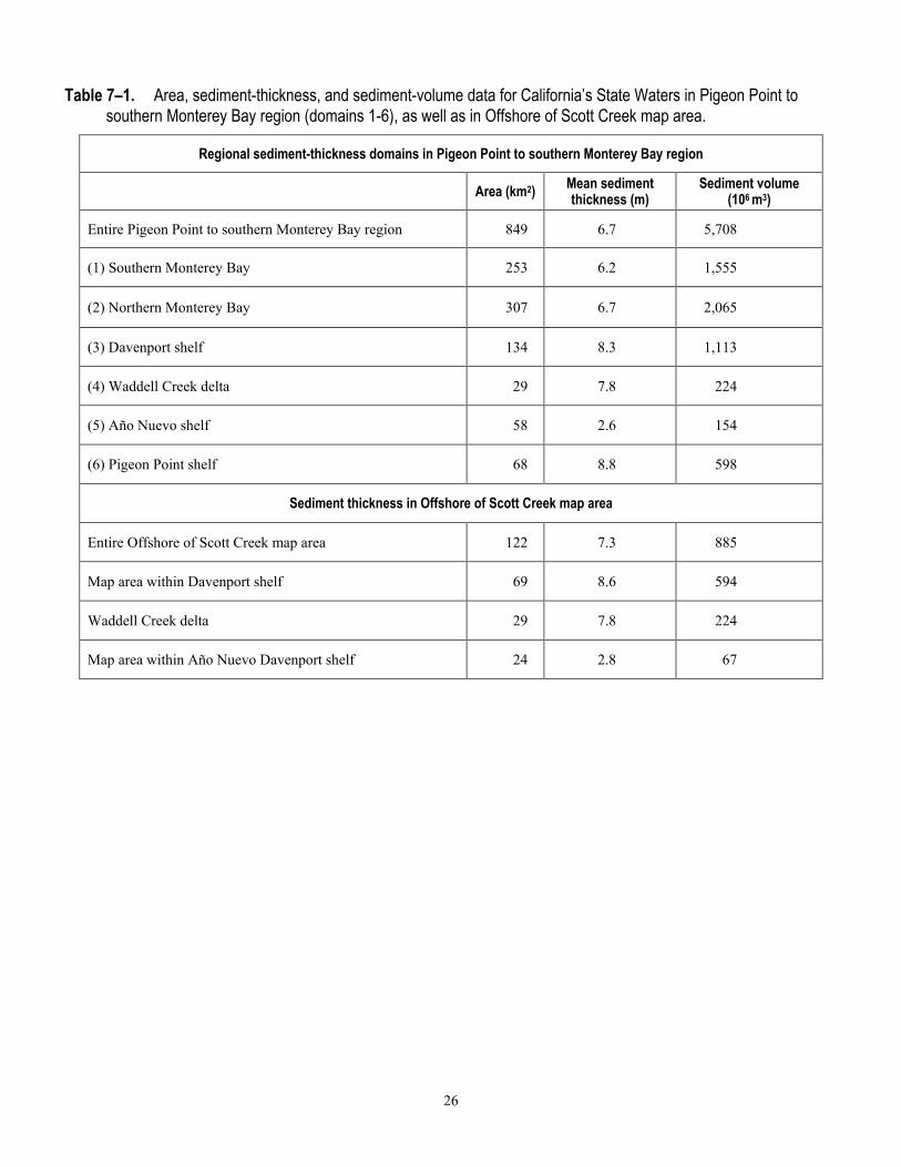
26

Table 7–1. Area, sediment-thickness, and sediment-volume data for California’s State Waters in Pigeon Point to southern Monterey Bay region (domains 1-6), as well as in Offshore of Scott Creek map area.

Regional sediment-thickness domains in Pigeon Point to southern Monterey Bay region

Area (km2) Mean sediment thickness (m)

Sediment volume (106 m3)

Entire Pigeon Point to southern Monterey Bay region 849 6.7 5,708

(1) Southern Monterey Bay 253 6.2 1,555

(2) Northern Monterey Bay 307 6.7 2,065

(3) Davenport shelf 134 8.3 1,113

(4) Waddell Creek delta 29 7.8 224

(5) Año Nuevo shelf 58 2.6 154

(6) Pigeon Point shelf 68 8.8 598

Sediment thickness in Offshore of Scott Creek map area

Entire Offshore of Scott Creek map area 122 7.3 885

Map area within Davenport shelf 69 8.6 594

Waddell Creek delta 29 7.8 224

Map area within Año Nuevo Davenport shelf 24 2.8 67

27

Chapter 8. Geologic and Geomorphic Map of the Offshore of Scott Creek Map Area (Sheet 10) By Samuel Y. Johnson, Stephen R. Hartwell, and Clifton W. Davenport

Geologic and Geomorphic Summary Marine geology and geomorphology were mapped in the Offshore of Scott Creek map area from

approximate Mean High Water (MHW) to the 3-nautical-mile limit of California’s State Waters. MHW is defined at an elevation of 1.46 m above the North American Vertical Datum of 1988 (NAVD 88) (Weber and others, 2005). Offshore geologic units were delineated on the basis of integrated analyses of adjacent onshore geology with multibeam bathymetry and backscatter imagery (sheets 1, 2, 3), seafloor-sediment and rock samples (Reid and others, 2006), digital camera and video imagery (sheet 6), and high-resolution seismic-reflection profiles (sheet 8). Aerial photographs taken in multiple years were used to map the nearshore area (0 to 10 m water depth) and to link the offshore and onshore geology. The relative proportions of all offshore map units are shown in table 8–1.

The onshore geology was compiled from Smith (1981), California Geological Survey (1982), Brabb (1997), and Graymer and others (2006); unit ages, which are from these sources, reflect local stratigraphic relations. In addition, some units were modified by C.W. Davenport on the basis of analysis of 2009 lidar imagery.

The offshore part of the map area lies southwest of the southwest flank of the Santa Cruz Mountains, extending from the shoreline to water depths of about 60 to 75 m on the gently dipping (about 0.6° to 0.8°) continental shelf. The shelf is underlain by Neogene bedrock and a variably thick (as much as 24 m) upper Quaternary sediment cover (see sheet 9). Sea level has risen about 120 to 130 m during the last about 21,000 years (see, for example, Stanford and others, 2011), leading to broadening of the continental shelf, progressive eastward migration of the shoreline and wave-cut platform, and associated transgressive erosion and deposition of sediment (see, for example, Catuneanu, 2006). The Offshore of Scott Creek map area is now an open-ocean shelf that is subjected to full, and sometimes severe, wave energy. Shelf morphology and geology also are affected by local faulting, folding, uplift, and possibly subsidence.

The Offshore of Scott Creek map area straddles the right-lateral San Gregorio Fault Zone, an important structure in the distributed transform boundary between the North American and Pacific plates (see, for example, Dickinson and others, 2005). This fault zone is part of a regional fault system that is present predominantly in the offshore for about 400 km, from Point Conception in the south (where it is known as the Hosgri Fault; Johnson and Watt, 2012) to Bolinas and Point Reyes in the north (Bruns and others, 2002; Ryan and others, 2008). The San Gregorio Fault Zone in the map area is part of a 90-km-long offshore segment that extends northward from Point Sur (about 75 km south of the map area), across outer Monterey Bay to Point Año Nuevo (1 km north of the map area) (see sheet 9; see also, Weber and Lajoie, 1980; Brabb and others, 1998; Wagner and others, 2002). Offshore parts of this fault zone are identified in seismic-reflection profiles on the basis of abrupt truncation or warping of reflections and (or) the juxtaposition of reflection panels that have differing seismic parameters (see sheet 8). In this map area, the San Gregorio Fault forms a distributed shear zone about 2 km wide that includes two main fault strands. The nearshore east strand, known as the Coastways Fault, partly coincides with a prominent bathymetric lineament on the outer flank of nearshore bedrock outcrops present between Davenport and the mouth of Waddell Creek (see sheets 1, 2). The west strand, known as the Frijoles Fault, cuts across the flat, sediment-covered shelf. Cumulative lateral slip on the San Gregorio Fault Zone is thought to range from 4 to 10 mm/yr on the basis of field observations at Point Año Nuevo (Weber, 1994).

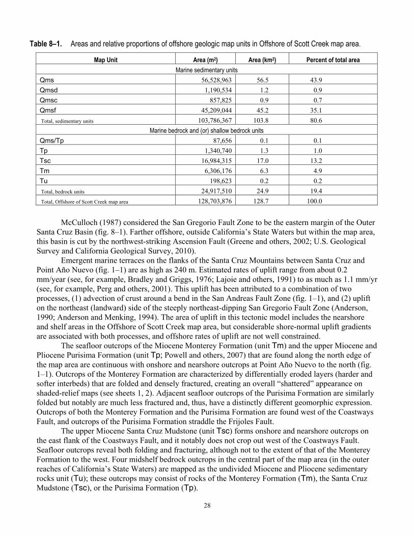
28

Table 8–1. Areas and relative proportions of offshore geologic map units in Offshore of Scott Creek map area.

Map Unit Area (m2) Area (km2) Percent of total area Marine sedimentary units

Qms 56,528,963 56.5 43.9 Qmsd 1,190,534 1.2 0.9 Qmsc 857,825 0.9 0.7 Qmsf 45,209,044 45.2 35.1 Total, sedimentary units 103,786,367 103.8 80.6

Marine bedrock and (or) shallow bedrock units Qms/Tp 87,656 0.1 0.1 Tp 1,340,740 1.3 1.0 Tsc 16,984,315 17.0 13.2 Tm 6,306,176 6.3 4.9 Tu 198,623 0.2 0.2 Total, bedrock units 24,917,510 24.9 19.4 Total, Offshore of Scott Creek map area 128,703,876 128.7 100.0

McCulloch (1987) considered the San Gregorio Fault Zone to be the eastern margin of the Outer

Santa Cruz Basin (fig. 8–1). Farther offshore, outside California’s State Waters but within the map area, this basin is cut by the northwest-striking Ascension Fault (Greene and others, 2002; U.S. Geological Survey and California Geological Survey, 2010).

Emergent marine terraces on the flanks of the Santa Cruz Mountains between Santa Cruz and Point Año Nuevo (fig. 1–1) are as high as 240 m. Estimated rates of uplift range from about 0.2 mm/year (see, for example, Bradley and Griggs, 1976; Lajoie and others, 1991) to as much as 1.1 mm/yr (see, for example, Perg and others, 2001). This uplift has been attributed to a combination of two processes, (1) advection of crust around a bend in the San Andreas Fault Zone (fig. 1–1), and (2) uplift on the northeast (landward) side of the steeply northeast-dipping San Gregorio Fault Zone (Anderson, 1990; Anderson and Menking, 1994). The area of uplift in this tectonic model includes the nearshore and shelf areas in the Offshore of Scott Creek map area, but considerable shore-normal uplift gradients are associated with both processes, and offshore rates of uplift are not well constrained.

The seafloor outcrops of the Miocene Monterey Formation (unit Tm) and the upper Miocene and Pliocene Purisima Formation (unit Tp; Powell and others, 2007) that are found along the north edge of the map area are continuous with onshore and nearshore outcrops at Point Año Nuevo to the north (fig. 1–1). Outcrops of the Monterey Formation are characterized by differentially eroded layers (harder and softer interbeds) that are folded and densely fractured, creating an overall “shattered” appearance on shaded-relief maps (see sheets 1, 2). Adjacent seafloor outcrops of the Purisima Formation are similarly folded but notably are much less fractured and, thus, have a distinctly different geomorphic expression. Outcrops of both the Monterey Formation and the Purisima Formation are found west of the Coastways Fault, and outcrops of the Purisima Formation straddle the Frijoles Fault.

The upper Miocene Santa Cruz Mudstone (unit Tsc) forms onshore and nearshore outcrops on the east flank of the Coastways Fault, and it notably does not crop out west of the Coastways Fault. Seafloor outcrops reveal both folding and fracturing, although not to the extent of that of the Monterey Formation to the west. Four midshelf bedrock outcrops in the central part of the map area (in the outer reaches of California’s State Waters) are mapped as the undivided Miocene and Pliocene sedimentary rocks unit (Tu); these outcrops may consist of rocks of the Monterey Formation (Tm), the Santa Cruz Mudstone (Tsc), or the Purisima Formation (Tp).

29

Modern nearshore and inner shelf to midshelf sediments are mostly sand (unit Qms) and a mix of sand and gravel (units Qmsc and Qmsd). Unit Qms notably is also present in well-defined channels that cut through nearshore bedrock exposures at the mouths of Waddell Creek, Scott Creek, Agua Puera Creek, and San Vicente Creek (fig. 1–2). These distinct channels, which extend to water depths of 20 to 40 m, were formed by subaerial erosion during sea-level lowstands (Anima and others, 2002). The coarser grained sands and gravels (units Qmsc and Qmsd) are recognized primarily on the basis of bathymetry and (or) high backscatter (see sheets 1, 2, 3). Unit Qmsc mainly is found adjacent to bedrock, in water depths of less than 40 m.

Unit Qmsd typically is mapped as erosional lags in scour depressions (see, for example, Cacchione and others, 1984) that are bounded by relatively sharp or, less commonly, diffuse contacts with the horizontal sand sheets of unit Qms. These depressions typically are irregular to lenticular and a few tens of centimeters deep, and they range in size from a few tens of square meters to as much as about 290,000 m2. They most commonly are found adjacent to seafloor bedrock exposures, at water depths that range from about 15 to 55 m. Such scour depressions are common along this stretch of the California coast (see, for example, Cacchione and others, 1984; Hallenbeck and others, 2012; Davis and others, 2013), where offshore sandy sediment can be relatively thin (and, thus, is unable to fill the depressions) owing to low sediment supply from rivers and also to significant erosion and offshore transport of sediment during large northwest winter swells. Such features have been referred to as “rippled scour depressions” (see, for example, Cacchione and others, 1984) or “sorted bedforms” (see, for example, Goff and others, 2005; Trembanis and Hume, 2011). Although the general areas in which both unit Qmsd scour depressions and surrounding Qms sand sheets are found are not likely to change substantially, the boundaries of the unit(s) likely are ephemeral, changing seasonally and during significant storm events.

An offshore transition from unit Qms to the finer grained marine sediments of unit Qmsf is present at water depths of 50 to 65 m. Unit Qmsf primarily consists of mud and muddy sand and commonly is extensively bioturbated. These fine-grained shelf sediments are derived from local coastal watersheds, bluff erosion, and the northward advection of sediment from fluvial sources within Monterey Bay (Edwards, 2002; Grossman and others, 2006).

In areas where shelf sediments form thin (less than 2.5 m) veneers over low-relief rocks of the upper Miocene and Pliocene Purisima Formation, composite unit Qms/Tp is mapped. This composite unit is recognized on the basis of the combination of flat relief, continuity with moderate- to high-relief bedrock outcrops, and moderate to high backscatter (see sheet 3). Overlying sediment is interpreted as an ephemeral and dynamic sediment layer that may or may not be continuously present, depending on storms, seasonal and (or) annual patterns of sediment movement, or longer term climate cycles. Storlazzi and others (2011) described the seasonal burial and exhumation of submerged bedrock in a similar high-energy setting in northern Monterey Bay, just south of the map area.

30

Figure 8–1. Schematic map showing major offshore structural features northwest of Monterey Bay (modified from McCulloch, 1987; Greene and others, 2002; Dickinson, 2005). Red box shows Offshore of Scott Creek map area. Yellow line shows limit of California’s State Waters. Outer Santa Cruz Basin (modified from McCulloch, 1987) shown by blue shading and hachured lines (hachures point into basin). Solid black lines show traces of faults: AF, Ascension Fault (sawteeth on upper plate); CF, Coastways Fault; FF, Frijoles Fault; SGFZ, San Gregorio Fault Zone (also shown by dark-gray shading); SAF, San Andreas Fault; ZYF, Zayante-Vergeles Fault. Dashed magenta lines show axes of structural highs: PPH, Pigeon Point high; SCH, Santa Cruz high. Other abbreviations: PAN, Point Año Nuevo; PP, Pigeon Point.

31

DESCRIPTION OF MAP UNITS

OFFSHORE GEOLOGIC AND GEOMORPHIC UNITS

[Note that, where older units (typically, bedrock) are overlain by thin (<1 m thick) Quaternary deposits, composite units are mapped. These composite units, which are shown with gray stipple pattern on older unit, are designated by composite label indicating both overlying sediment cover and lower (older) unit, separated by slash (for example, Qms/Tp indicates that thin sheet of Qms overlies Tp)] Qms Marine nearshore and shelf deposits (late Holocene)—Predominantly sand; ripple marks

common; found on gently seaward-dipping (about 0.6° to 0.8°) surface that extends from shoreline to water depths of about 50 to 65 m

Qmsd Marine shelf scour depressions (late Holocene)—Inferred to be coarse sand and possibly gravel; generally found as single depressions or in groups of depressions interspersed with elevated shelf sediments (unit Qms), adjacent to and (or) offshore of bedrock outcrops. Depressions typically have curved to irregular margins and diffuse to sharp boundaries, and they typically are 15 to 50 cm deep. In map area, backscatter data show intensity contrasts that suggest depressions are filled with sediment that is coarser than intervening elevated sandy shelf deposits. General area in which unit is found is not likely to change substantially, but boundaries of unit(s) and locations of individual depressions (and intervening flat sheets) likely are ephemeral, changing during significant storm events

Qmsc Coarse-grained marine nearshore and shelf deposits (late Holocene)—Predominantly coarse sand and gravel

Qmsf Fine-grained marine shelf deposits (late Holocene)—Predominantly mud to muddy sand; commonly bioturbated; found on gently seaward-dipping (less than 1°) surfaces, in water depths greater than about 50 to 65 m

Tp Purisima Formation (Pliocene and late Miocene)—Medium-grained to very fine-grained, poorly indurated to friable, marine sandstone, siltstone, and claystone; also includes conglomerate lenses and a few beds of white volcanic ash. Stippled areas (composite unit Qms/Tp) indicate where thin sheets of Qms overlie unit. Age is based on biostratigraphic and geochronologic data summarized by Powell and others (2007)

Tu Sedimentary rocks, undivided (Pliocene and Miocene)—May consist of rocks of the Purisima Formation (Tp), the Santa Cruz Mudstone (Tsc), or the Monterey Formation (Tm)

Tsc Santa Cruz Mudstone (late Miocene)—Siliceous organic mudstone and nonsiliceous mudstone, siltstone, and minor amounts of sandstone

Tm Monterey Formation (late and middle Miocene)—Porcelaneous shale and chert, porcelaneous mudstone, calcareous claystone, and small amounts of siltstone and sandstone

ONSHORE GEOLOGIC AND GEOMORPHIC UNITS

[Units compiled from Smith (1981), California Geological Survey (1982), Brabb (1997), and Graymer and others (2006); unit ages, which are from these sources, reflect local stratigraphic relations. In addition, some units modified by C.W. Davenport on basis of analysis of 2009 lidar imagery] af Artificial fill (late Holocene)—Material placed by humans Qc Stream-channel deposits (late Holocene)—Sand and gravel deposits within active stream

channels

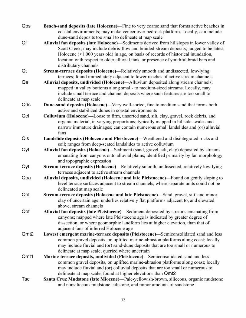
32

Qbs Beach-sand deposits (late Holocene)—Fine to very coarse sand that forms active beaches in coastal environments; may make veneer over bedrock platform. Locally, can include dune-sand deposits too small to delineate at map scale

Qf Alluvial fan deposits (late Holocene)—Sediments derived from hillslopes in lower valley of Scott Creek; may include debris-flow and braided-stream deposits; judged to be latest Holocene (<1,000 years old) in age, on basis of records of historical inundation, location with respect to older alluvial fans, or presence of youthful braid bars and distributary channels

Qt Stream-terrace deposits (Holocene)—Relatively smooth and undissected, low-lying terraces; found immediately adjacent to lower reaches of active stream channels

Qa Alluvial deposits, undivided (Holocene)—Alluvium deposited along stream channels; mapped in valley bottoms along small- to medium-sized streams. Locally, may include small terrace and channel deposits where such features are too small to delineate at map scale

Qds Dune-sand deposits (Holocene)—Very well-sorted, fine to medium sand that forms both active and stabilized dunes in coastal environments

Qcl Colluvium (Holocene)—Loose to firm, unsorted sand, silt, clay, gravel, rock debris, and organic material, in varying proportions; typically mapped in hillside swales and narrow immature drainages; can contain numerous small landslides and (or) alluvial fans

Qls Landslide deposits (Holocene and Pleistocene)—Weathered and disintegrated rocks and soil; ranges from deep-seated landslides to active colluvium

Qyf Alluvial fan deposits (Holocene)—Sediment (sand, gravel, silt, clay) deposited by streams emanating from canyons onto alluvial plains; identified primarily by fan morphology and topographic expression

Qyt Stream-terrace deposits (Holocene)—Relatively smooth, undissected, relatively low-lying terraces adjacent to active stream channels

Qoa Alluvial deposits, undivided (Holocene and late Pleistocene)—Found on gently sloping to level terrace surfaces adjacent to stream channels, where separate units could not be delineated at map scale

Qot Stream-terrace deposits (Holocene and late Pleistocene)—Sand, gravel, silt, and minor clay of uncertain age; underlies relatively flat platforms adjacent to, and elevated above, stream channels

Qof Alluvial fan deposits (late Pleistocene)—Sediment deposited by streams emanating from canyons; mapped where late Pleistocene age is indicated by greater degree of dissection, or where geomorphic landform lies at higher elevation, than that of adjacent fans of inferred Holocene age

Qmt2 Lowest emergent marine-terrace deposits (Pleistocene)—Semiconsolidated sand and less common gravel deposits, on uplifted marine-abrasion platforms along coast; locally may include fluvial and (or) sand-dune deposits that are too small or numerous to delineate at map scale; queried where uncertain

Qmt1 Marine-terrace deposits, undivided (Pleistocene)—Semiconsolidated sand and less common gravel deposits, on uplifted marine-abrasion platforms along coast; locally may include fluvial and (or) colluvial deposits that are too small or numerous to delineate at map scale; found at higher elevations than Qmt2

Tsc Santa Cruz Mudstone (late Miocene)—Pale-yellowish-brown, siliceous, organic mudstone and nonsiliceous mudstone, siltstone, and minor amounts of sandstone

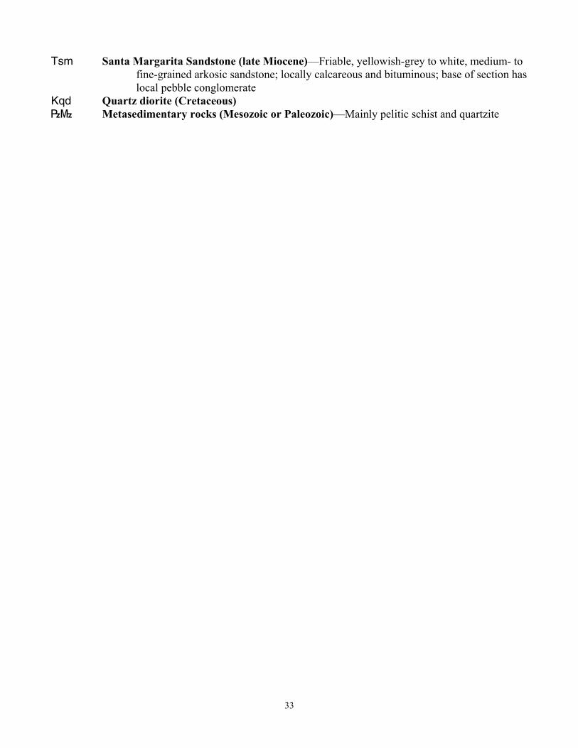
33

Tsm Santa Margarita Sandstone (late Miocene)—Friable, yellowish-grey to white, medium- to fine-grained arkosic sandstone; locally calcareous and bituminous; base of section has local pebble conglomerate

Kqd Quartz diorite (Cretaceous) Metasedimentary rocks (Mesozoic or Paleozoic)—Mainly pelitic schist and quartzite

34

Acknowledgments This publication was funded by the California Ocean Protection Council and the U.S. Geological

Survey (USGS) Coastal and Marine Geology Program. We thank the officers, crew, and scientific parties of the ships—R/V VenTresca, California State University, Monterey Bay, Seafloor Mapping Lab; F/V Quicksilver, Fugro Pelagos; and R/V Parke Snavely, USGS Pacific Coastal and Marine Science Center—for their skill and professionalism in collecting the data presented in this report. We thank Mary Young (University of California, Santa Cruz) and Robert Peters (USGS) for their critical reviews that greatly improved this report. We are very grateful to USGS editor Taryn Lindquist for helping us develop the templates and formats for this series of publications, and for invaluable editorial review and suggestions.

35

References Cited Ainley, D.B., and Hyrenbach, K.D., 2010, Top-down and bottom-up factors affecting seabird population

trends in the California current system (1985-2006): Progress in Oceanography, v. 84, p. 242–254. Anderson, R.S., 1990, Evolution of the northern Santa Cruz Mountains by advection of crust past a San

Andreas Fault bend: Science, v. 249, p. 397–401. Anderson, R.S., and Menking, K.M., 1994, The Quaternary marine terraces of Santa Cruz, California—

Evidence for coseismic uplift on two faults: Geological Society of America Bulletin, v. 106, p. 649–664.

Anderson, T.J., Cochrane, G.R., Roberts, D.A., Chezar, H., and Hatcher, G., 2007, A rapid method to characterize seabed habitats and associated macro-organisms, in Todd, B.J., and Greene, H.G., eds., Mapping the seafloor for habitat characterization: Geological Association of Canada Special Paper 47, p. 71–79.

Anima, R.J., Eittreim, S.L., Edwards, B.D., and Stevenson, A.J., 2002, Nearshore morphology and late Quaternary geologic framework of the northern Monterey Bay Marine Sanctuary, California: Marine Geology, v. 181, p. 35–54.

Brabb, E.E., 1997, Geologic map of Santa Cruz County, California—A digital database: U.S. Geological Survey Open-File Report 97–489, scale 1:62,500, available at http://pubs.usgs.gov/of/1997/of97-489/.

Brabb, E.E., Graymer, R.W., and Jones, D.L., 1998, Geology of the onshore part of San Mateo County, California—A digital database: U.S. Geological Survey Open-File Report 98–137, scale 1:62,500, available at http://pubs.usgs.gov/of/1998/of98-137/.

Bradley, W.C., and Griggs, G.B., 1976, Form, genesis, and deformation of central California wave-cut platforms: Geological Society of America Bulletin, v. 87, p. 433–449.

Briggs, J.C., 1974, Marine zoogeography: New York, McGraw-Hill, 480 p. Bruns, T.R., Cooper, A.K., Carlson, P.R., and McCulloch, D.S., 2002, Structure of the submerged San

Andreas and San Gregorio Fault zones in the Gulf of Farallones as inferred from high-resolution seismic-reflection data, in Parsons, T., ed., Crustal structure of the coastal and marine San Francisco Bay region, California: U.S. Geological Survey Professional Paper 1658, p. 77–117, available at http://pubs.usgs.gov/pp/1658/.

Cacchione, D.A., Drake, D.E., Grant, W.D., and Tate, G.B., 1984, Rippled scour depressions of the inner continental shelf off central California: Journal of Sedimentary Petrology, v. 54, p. 1,280–1,291.

Calambokidis, J., and Barlow, J., 2004, Abundance of blue and humpback whales in the eastern North Pacific estimated by capture-recapture and line-transect methods: Marine Mammal Science, v. 20, p. 63–85.

California Department of Fish and Wildlife, 2008, California Marine Life Protection Act master plan for marine protected areas—Revised draft: California Department of Fish and Wildlife [formerly California Department of Fish and Game], available at http://www.dfg.ca.gov/mlpa/masterplan.asp.

California Geological Survey, 1982, Alquist-Priolo earthquake fault zone map of Año Nuevo quadrangle: California Geological Survey, State of California Special Studies Zone Map, scale 1:24,000, available at http://www.quake.ca.gov/gmaps/WH/regulatorymaps.htm.

California Geological Survey, 2002, California geomorphic provinces: California Geologic Survey Note 36, 4 p.

Catuneanu, O., 2006, Principles of sequence stratigraphy: Amsterdam, Elsevier, 375 p. Chin, J.L., Clifton, H.E., and Mullins, H.T., 1988, Seismic stratigraphy and late Quaternary shelf

history, south-central Monterey Bay, California: Marine Geology, v. 81, p. 137–157. Cochrane, G.R., 2008, Video-supervised classification of sonar data for mapping seafloor habitat, in

Reynolds, J.R., and Greene, H.G., eds., Marine habitat mapping technology for Alaska: Fairbanks, University of Alaska, Alaska Sea Grant College Program, p. 185–194, available at

36

http://doc.nprb.org/web/research/research%20pubs/615_habitat_mapping_workshop/Individual%20Chapters%20High-Res/Ch13%20Cochrane.pdf.

Cochrane, G.R., Conrad, J.E., Reid, J.A., Fangman, S., and Golden, N., 2005, Nearshore benthic habitat GIS for the Channel Islands National Marine Sanctuary and southern California state fisheries reserves, vol. II: U.S. Geological Survey Open-File Report 2005–1170, available at http://pubs.usgs.gov/of/2005/1170/.

Cochrane, G.R., and Lafferty, K.D., 2002, Use of acoustic classification of sidescan sonar data for mapping benthic habitat in the Northern Channel Islands, California: Continental Shelf Research, v. 22, p. 683–690.

Cochrane, G.R., Nasby, N.M., Reid, J.A., Waltenberger, B., and Lee, K.M., 2003, Nearshore benthic habitat GIS for the Channel Islands National Marine Sanctuary and southern California state fisheries reserves, vol. I: U.S. Geological Survey Open-File Report 03–85, available at http://pubs.usgs.gov/ of/2003/0085/.

Collins, C.A., Garfield, N., Rago, T.A., Rischmiller, F.W., and Carter, E., 2000, Mean structure of the inshore counter-current and California undercurrent off Point Sur, California: Deep-Sea Research II, v. 47, p. 765–782.

Davis, A.C.D., Kvitek, R.G., Mueller, C.B.A., Young, M.A., Storlazzi, C.D., and Phillips, E.L., 2013, Distribution and abundance of rippled scour depressions along the California coast: Continental Shelf Research, v. 69, p. 88–100, doi:10.1016/j.csr.2013.09.010.

Dawson, M.N., Waples, R.S., and Bernardi, G., 2006, Phylogeography, in Allen, L.G., Pondella, D.J., II, and Horn, M.H., eds., The ecology of marine fishes, California and adjacent waters: Berkeley, University of California Press, 660 p.

Dickinson, W.R., 2004, Evolution of the North American cordillera: Annual Reviews of Earth and Planetary Sciences, v. 32, p. 13–45.

Dickinson, W.R., Ducea, M., Rosenberg, L.I., Greene, H.G., Graham, S.A., Clark, J.C., Weber, G.E., Kidder, S., Ernst, W.G., and Brabb, E.E., 2005, Net dextral slip, Neogene San Gregorio–Hosgri fault zone, coastal California—Geologic evidence and tectonic implications: Geological Society of America Special Paper 391, 43 p.

Edwards, B.D., 2002, Variations in sediment texture on the northern Monterey Bay National Marine Sanctuary continental shelf: Marine Geology, v. 181, p. 83–100.

Eittreim, S.L., Anima, R.J., and Stevenson, A.J., 2002, Seafloor geology of the Monterey Bay area continental shelf: Marine Geology, vol. 181, p. 3–34.

Goff, J.A., Mayer, L.A., Traykovski, P., Buynevich, I., Wilkens, R., Raymond, R., Glang, G., Evans, R.L., Olson, H., and Jenkins, C., 2005, Detailed investigations of sorted bedforms or “rippled scour depressions,” within the Martha’s Vineyard Coastal Observatory, Massachusetts: Continental Shelf Research, v. 25, p. 461–484, doi:10.1016/j.csr.2004.09.019.

Graymer, R.W., Moring, B.C., Saucedo, G.J., Wentworth, C.M., Brabb, E.E., and Knudsen, K.L., 2006, Geologic map of the San Francisco Bay region: U.S. Geological Survey Scientific Investigations Map 2918, available at http://pubs.usgs.gov/sim/2006/2918/.

Greene, H.G., 1977, Geology of the Monterey Bay region: U.S. Geological Survey Open-File Report 77–718, 347 p.

Greene, H.G., 1990, Regional tectonics and structural evolution of the Monterey Bay region, central California, in Garrison, R.E., Greene, H.G., Hicks, K.R., Weber, G.E., and Wright, T.L., eds., Geology and tectonics of the central California coastal region, San Francisco to Monterey: American Association of Petroleum Geologists, Pacific Section, Guidebook GB67, p. 31–56.

Greene, H.G., Bizzarro, J.J., O’Connell, V.M., and Brylinsky, C.K., 2007, Construction of digital potential marine benthic habitat maps using a coded classification scheme and its application, in Todd,

37

B.J., and Greene, H.G., eds., Mapping the seafloor for habitat characterization: Geological Association of Canada Special Paper 47, p. 141–155.

Greene, H.G., Bizzarro, J.J., Tilden, J.E., Lopez, H.L., and Erdey, M.D., 2005, The benefits and pitfalls of geographic information systems in marine benthic habitat mapping, in Wright, D.J., and Scholz, A.J., eds., Place matters: Portland, Oregon State University Press, p. 34–46.

Greene, H.G., Maher, N.M., and Paull, C.K., 2002, Physiography of the Monterey Bay National Marine Sanctuary and implications about continental margin development: Marine Geology, v. 181, p. 55–82.

Greene, H.G., Yoklavich, M.M., Starr, R.M., O’Connell, V.M., Wakefield, W.W., Sullivan, D.E., McRea, J.E., and Cailliet, G.M., 1999, A classification scheme for deep seafloor habitats: Oceanologica Acta, v. 22, p. 663–678.

Griggs, G., Patsch, K., and Savoy, L., 2005, Living with the changing California coast: Berkeley, University of California Press, 540 p.

Grossman, E.E., Eittreim, S.L., Field, M.E., and Wong, F.L., 2006, Shallow stratigraphy and sedimentation history during high-frequency sea-level changes on the central California shelf: Continental Shelf Research, v. 26, p. 1,217–1,239, doi:10.1016/j.csr.2006.04.001.

Hallenbeck, T.R., Kvitek, R.G., and Lindholm, J., 2012, Rippled scour depressions add ecologically significant heterogeneity to soft-bottom habitats on the continental shelf: Marine Ecology Progress Series, v. 468, p. 119–133, doi:10.3354/meps09948.

Hapke, C.J., Reid, D., Richmond, B.B., Ruggiero, P., and List, J., 2006, National assessment of shoreline change, part 3—Historical shoreline change and associated coastal land loss along sandy shorelines of the California coast: U.S. Geological Survey Open-File Report 2006–1219, 72 p., available at http://pubs.usgs.gov/of/2006/1219/.

Inman, D.L., and Jenkins, D.A., 1999, Climate change and the episodicity of sediment flux of small California rivers: Journal of Geology, v. 107, p. 251–270.

Johnson, S.Y., and Watt, J.T., 2012, Influence of fault trend, bends, and convergence on shallow structure and geomorphology of the Hosgri strike-slip fault, offshore Central California: Geosphere, v. 8, p. 1,632–1,656, doi:10.1130/GES00830.1.

Koehl, M.A.R., and Wainwright, S.A., 1977, Mechanical adaptations of a giant kelp: Limnology and Oceanography, v. 22, p. 1,067–1,071.

Kvitek, R., Bretz, C., Cochrane, G., and Greene, H.G., 2006, Final report, Statewide Marine Mapping Planning Workshop, December 12–13, 2005, Seaside, Calif.: California State University, Monterey Bay, 108 p., available at http://euclase.csumb.edu/DATA_DOWNLOAD/StrategicMapgWrkshp05/ MappingWorkshop12_12-13/Final_Report/CA Habitat Mapping Rpt.pdf.

Kvitek, R.G., Phillips, E.L., and Dartnell, P., 2012, Colored shaded-relief bathymetry, Hueneme Canyon and vicinity, California, sheet 1 in Johnson, S.Y., Dartnell, P., Cochrane, G.R., Golden, N.E., Phillips, E.L., Ritchie, A.C., Kvitek, R.G., Greene, H.G., Krigsman, L.M., Endris, C.A., Clahan, K.B., Sliter, R.W., Wong, F.L., Yoklavich, M.M., and Normark, W.R. (S.Y. Johnson, ed.), California State Waters Map Series—Hueneme Canyon and vicinity, California: U.S. Geological Survey Scientific Investigations Map 3225, pamphlet 41 p., 12 sheets, available at http://pubs.usgs.gov/sim/3225/.

Lajoie, K.R., Ponti, D.J., Powell, C.L., II, Mathieson, S.A., and Sarna-Wojcicki, A.M., 1991, Emergent marine strandlines and associated sediments, coastal California—A record of Quaternary sea-level fluctuations, vertical tectonic movements, climatic changes, and coastal processes, in Morrison, R.B., ed., The Geology of North America, Quaternary nonglacial geology—Conterminous U.S.: Geological Society of America, Decade of North American Geology, v. K–2, p. 190–214.

Lynn, R.J., and Simpson, J.J., 1987, The California Current system—The seasonal variability of its physical characteristics: Journal of Geophysical Research, v. 92, p. 12,947–12,966.

38

Madden, C.J., Goodin, K.L., Allee, R., Finkbeiner, M., and Bamford, D.E., 2008, Draft Coastal and Marine Ecological Classification Standard: National Oceanic and Atmospheric Administration (NOAA) and NatureServe, v. III, 77 p.

McCulloch, D.S., 1987, Regional geology and hydrocarbon potential of offshore central California, in Scholl, D.W., Grantz, A., and Vedder, J.G., eds., Geology and resource potential of the continental margin of western North America and adjacent ocean basins—Beaufort Sea to Baja California: Circum-Pacific Council for Energy and Mineral Resources, Earth Science Series, v. 6, p. 353–401.

McGowan, J.A., Cayan, D.R., and Korman, L.M., 1998, Climate-ocean variability and ecosystem response in the Northeast Pacific: Science, v. 281, p. 210–217.

Miller, K.A., and Estes, J.A., 1989, Western range extension for Nereocystis luetkeana in the North Pacific Ocean: Botanica Marina, v. 32, p. 535–538.

Mitchum, R.M., Jr., Vail, P.R., and Sangree, J.B., 1977, Seismic stratigraphy and global changes of sea level, part 6—Stratigraphic interpretation of seismic reflection patterns in depositional sequences, in Payton, C.E., ed., Seismic stratigraphy—Applications to hydrocarbon exploration: Tulsa, Okla., American Association of Petroleum Geologists, p. 117–133.

Mullins, H.T., Nagel, D.K., and Dominguez, L.L., 1985, Tectonic and eustatic controls of late Quaternary shelf sedimentation along the central California (Santa Cruz) continental margin—High-resolution seismic stratigraphic evidence: Sedimentary Geology, v. 45, p. 327–347.

Murray, A.B., and Thieler, E.R., 2004, A new hypothesis and exploratory model for the formation of large-scale inner-shelf sediment sorting and “rippled scour depressions:” Continental Shelf Research, v. 24, no. 3, p. 295–315.

Northern California Earthquake Data Center, 2014, Northern California earthquake catalog: Northern California Earthquake Data Center database, accessed April 5, 2014, at http://www.ncedc.org/ncsn/.

Peltier, W.R., and Fairbanks, R.G., 2006, Global glacial ice volume and Last Glacial Maximum duration from an extended Barbados sea level record: Quaternary Science Reviews, v. 25, p. 3,322–3,337.

Perg, L.A., Anderson, R.S., and Finkel, R.C., 2001, Use of a new 10Be and 26Al inventory to data marine terraces, Santa Cruz, California, USA: Geology, v. 29, p. 879–882.

Petersen, M.D., Moschetti, M.P., Powers, P.M., Mueller, C.S., Haller, K.M., Frankel, A.D., Zeng, Yuehua, Rezaeian, Sanaz, Harmsen, S.C., Boyd, O.S., Field, Ned, Chen, Rui, Rukstales, K.S., Luco, Nico, Wheeler, R.L., Williams, R.A., and Olsen, A.H., 2014, Documentation for the 2014 update of the United States national seismic hazard maps: U.S. Geological Survey Open-File Report 2014–1091, 243 p., available at http://dx.doi.org/10.3133/ofr20141091.

Phillips, E.L., Storlazzi, C.D., Dartnell, P., and Edwards, B.D., 2007, Exploring rippled scour depressions offshore Huntington Beach, CA: Coastal Sediments 2007, v. 3, p. 1,851–1,864.

Powell, C.L., II, Barron, J.A., Sarna-Wojcicki, A.M., Clark, J.C., Perry, F.A., Brabb, E.E., and Fleck, R.J., 2007, Age, stratigraphy, and correlations of the late Neogene Purisima Formation, central California Coast Ranges: U.S. Geological Survey Professional Paper 1740, 32 p., available at http://pubs.usgs.gov/pp/2007/1740/.

Reid, J.A., Reid, J.M., Jenkins, C.J., Zimmerman, M., Williams, S.J., and Field, M.E., 2006, usSEABED —Pacific Coast (California, Oregon, Washington) offshore surficial-sediment data release: U.S. Geological Survey Data Series 182, available at http://pubs.usgs.gov/ds/2006/182/.

Ritchie, A.C., Finlayson, D.P., and Logan, J.B., 2010, Swath bathymetry surveys of the Monterey Bay area from Point Año Nuevo to Moss Landing, San Mateo, Santa Cruz, and Monterey Counties, California: U.S. Geological Survey Data Series 514, available at http://pubs.usgs.gov/ds/514/.

Ryan, H.F., Parsons, T., and Sliter, R.W., 2008. Vertical tectonic deformation associated with the San Andreas fault zone offshore of San Francisco, California: Tectonophysics, v. 429, p. 209–224, doi:10.1016/j.tecto.2008.06.011.

39

Smith, T.C., 1981, Fault evaluation report, Año Nuevo and Franklin Point quadrangles, California: California Division of Mines and Geology FER-116, April 1981, available at http://www.quake.ca.gov/gmaps/WH/regulatorymaps.htm.

Spalding, M.D., Fox, H.E., Allen, G.R., Davidson, N., Ferdana, Z.A., Finlayson, M., Halpern, B.S., Jorge, M.A., Lombana, A., Lourie, S.A., Martin, K.D., McManus, E., Molnar, J., Recchia, C.A., and Robertson, J., 2007, Marine ecoregions of the world—A bioregionalization of coastal and shelf areas: BioScience, v. 57, p. 573–583.

Spudich, P., ed., 1996, The Loma Prieta, California, earthquake of October 17, 1989—Main shock characteristics: U.S. Geological Survey Professional Paper 1550–A, 297 p., available at http://pubs.usgs.gov/pp/pp1550/pp1550a/.

Stanford, J.D., Hemingway, R., Rohling, E.J., Challenor, P.G., Medina-Elizalde, M., and Lester, A.J., 2011, Sea-level probability for the last deglaciation—A statistical analysis of far-field records: Global and Planetary Change, v. 79, p. 193–203, doi:10.1016/j.gloplacha.2010.11.002.

Stephens, J.S., Larson, R.J., and Pondella, D.J., II, 2006, Rocky reefs and kelp beds, in Allen, L.G., Pondella, D.J., II, and Horn, M.H., eds., The ecology of marine fishes, California and adjacent waters: Berkeley, University of California Press, 660 p.

Storlazzi, C.D., and Wingfield, D.K., 2005, Spatial and temporal variations in oceanographic and meteorologic forcing along the central California coast, 1980–2002: U.S. Geological Survey Scientific Investigations Report 2005–5085, 39 p., available at http://pubs.usgs.gov/sir/2005/5085/.

Storlazzi, C.D., Fregoso, T.A., Golden, N.E., and Finlayson, D.P., 2011, Sediment dynamics and the burial and exhumation of bedrock reefs along on emergent coastline as elucidated by repetitive sonar surveys, northern Monterey Bay, CA: Marine Geology, v. 289, p. 46–59.

Tinker, M.T., Doak, D.F., and Estes, J.A., 2008, Using demography and movement behavior to predict range expansion of the southern sea otter: Ecological Applications, v. 18, p. 1,781–1,794, doi:10.1890/07-0735.1.

Tissot, B.N., Yoklavich, M.M., Love, M.S., York, K., and Amend, M., 2006, Benthic invertebrates that form habitat on deep banks off southern California, with special reference to deep sea coral: Fishery Bulletin, v. 104, p. 167–181.

Trembanis, A.C., and Hume, T.M., 2011, Sorted bedforms on the inner shelf off northeastern New Zealand—Spatiotemporal relationships and potential paleo-environmental implications: Geo-Marine Letters, v. 31, p. 203–214, doi:10.1007/s00367-010-0225-8.

U.S. Geological Survey, 2009, National Archive of Marine Seismic Surveys: U.S. Geological Survey database, available at http://walrus.wr.usgs.gov/NAMSS/.

U.S. Geological Survey and California Geological Survey, 2010, Quaternary fault and fold database of the United States: U.S. Geological Survey database, accessed April 5, 2014, at http://earthquake.usgs.gov/hazards/qfaults/.

Waelbroeck, C., Labeyrie, L., Michel, E., Duplessy, J.C., McManus, J.F., Lambeck, K., Balbon, E., and Labracherie, M., 2002, Sea-level and deep water temperature changes derived from benthic foraminifera isotopic records: Quaternary Science Reviews, v. 21, p. 295–305.

Wagner, D.L., Greene, H.G., Saucedo, G.J., and Pridmore, C.L., 2002, Geologic map of the Monterey 30' × 60' quadrangle and adjacent areas, California: California Geological Survey Regional Geologic Map Series, scale 1:100,000, available at http://www.quake.ca.gov/gmaps/RGM/monterey/ monterey.html.

Watt, J.T., Hartwell, S.R., Johnson, S.Y., Sliter, R.W., Phillips, E.L., Ross, S.L., and Chin, J.L., 2014, Local (Offshore of San Gregorio map area) and regional (offshore from Bolinas to Pescadero) shallow-subsurface geology and structure, California, sheet 9 in Cochrane, G.R., Dartnell, P., Greene, H.G., Watt, J.T., Golden, N.E., Endris, C.A., Phillips, E.L., Hartwell, S.R., Johnson, S.Y., Kvitek, R.G., Erdey, M.D., Bretz, C.K., Manson, M.W., Sliter, R.W., Ross, S.L., Dieter, B.E., and Chin, J.L.

40

(G.R. Cochrane and S.A. Cochran, eds.), California State Waters Map Series—Offshore of San Gregorio, California: U.S. Geological Survey Scientific Investigations Map 3306, pamphlet 38 p., 10 sheets, scale 1:24,000, available at http://dx.doi.org/10.3133/sim3306.

Weber, G.E., 1990, Late Pleistocene slip rates on the San Gregorio fault zone at Point Año Nuevo, San Mateo County, California, in Greene, H.G., Weber, G.E., Wright, T.L., and Garrison, R.E., eds., Geology and tectonics of the central California coast region—San Francisco to Monterey: American Association of Petroleum Geologists, Pacific Section, volume and guidebook, v. 67, p. 193–204.

Weber, G.E., 1994, Late Pleistocene slip rates on the San Gregorio fault zone at Point Año Nuevo, San Mateo County, California, in Lettis, W.R., ed., Field trip guidebook—Transpressional deformation in the San Francisco Bay region: Friends of the Pleistocene, Pacific Southwest Cell, Guidebook, 1994 fall field trip, Sept. 30–Oct. 2, 1994, 101 p.

Weber, G.E., and Lajoie, K.R., 1980, Map of Quaternary faulting along the San Gregorio fault zone, San Mateo and Santa Cruz Counties, California: U.S. Geological Survey Open-File Report 80–907, 3 sheets, scale 1:24,000, available at http://pubs.er.usgs.gov/publication/ofr80907.

Weber, K.M., List, J.H., and Morgan, K.L.M., 2005, An operational mean high water datum for determination of shoreline position from topographic lidar data: U.S. Geological Survey Open-File Report 2005–1027, available at http://pubs.usgs.gov/of/2005/1027/.

Wentworth, C.K., 1922, A scale of grade and class terms for clastic sediments: Journal of Geology, v. 30, p. 377–392.

Wong, F.L., Phillips, E.L., Johnson, S.Y, and Sliter, R.W., 2012, Modeling of depth to base of Last Glacial Maximum and seafloor sediment thickness for the California State Waters Map Series, eastern Santa Barbara Channel, California: U.S. Geological Survey Open-File Report 2012–1161, 16 p., available at http://pubs.usgs.gov/of/2012/1161/.

Wright, D.J., Pendleton, M., Boulware, J., Walbridge, S., Gerlt, B., Eslinger, D., Sampson, D., and Huntley, E., 2012, ArcGIS Benthic Terrain Modeler (BTM), v. 3.0: Environmental Systems Research Institute and NOAA Coastal Services Center, Massachusetts Office of Coastal Zone Management, accessed February 1, 2013, at http://esriurl.com/5754.