Calibration of the Biological Condition Gradient for High ... · Calibration of the Biological...
86
Calibration of the Biological Condition Gradient for High Gradient Streams of Connecticut Prepared for: U.S. EPA Office of Science and Technology Connecticut Department of Environmental Protection By: Tetra Tech, Inc. 400 Red Brook Blvd. Suite 200 Owings Mills, MD 21117 August 2007 August 2007
Transcript of Calibration of the Biological Condition Gradient for High ... · Calibration of the Biological...

Calibration of the Biological Condition Gradient for High Gradient Streams of Connecticut
Prepared for: U.S. EPA Office of Science and Technology Connecticut Department of Environmental Protection By: Tetra Tech, Inc. 400 Red Brook Blvd. Suite 200 Owings Mills, MD 21117 August 2007 August 2007
CALIBRATION OF THE BIOLOGICAL
CONDITION GRADIENT FOR HIGH GRADIENT STREAMS OF CONNECTICUT
Prepared for:
U.S. EPA Office of Science and Technology Susan Jackson, Work Assignment Manager
Connecticut Department of Environmental Protection
Ernest Pizzuto
Prepared by:
Jeroen Gerritsen Ben Jessup
Tetra Tech, Inc. 400 Red Brook Boulevard, Suite 200
Owings Mills, MD 21117
August 2007
CT TALU Workshop Documentation
Tetra Tech, Inc. iii
EXECUTIVE SUMMARY In recent years, several states and the US EPA have developed a framework to support improved biological assessment. The framework, called Tiered Aquatic Life Use (TALU) supports development of tiered biological criteria in a state’s water quality standards that can protect the best quality waters, that can be used as a tool to prevent or remediate cumulative, incremental degradation, and that can help to establish realistic management goals for impaired waters. In recent years, several states and the US EPA have developed a framework to support improved biological assessment. The framework, called Tiered Aquatic Life Use (TALU), supports development of tiered biological criteria in a state’s water quality standards that can protect the best quality waters, that can be used as a tool to prevent or remediate cumulative, incremental degradation, and that can help to establish realistic management goals for impaired waters. The basis of the TALU framework is recognition that biological condition of water bodies responds to aggregate human-caused disturbance and stress, and that the biological condition can be measured reliably. For TALU implementation, biological condition is measured on the Biological Condition Gradient (BCG), a universal measurement system or yardstick that is calibrated on a common scale for all states and regions. This document describes the calibration of the BCG to high-gradient streams of Connecticut, which are routinely sampled in Connecticut DEP’s monitoring program. The BCG includes decision criteria to assign streams to levels of the BCG, and thus it can be directly applied to tiered aquatic life uses in Connecticut’s Criteria and Standards. The BCG is a more accurate and representative way to classify the condition of water bodies than previous methods, because its measurement standard is based on natural, undisturbed condition rather than a sliding scale of local conditions. Although it is intended to be a universal scale, it is not “one-size-fits-all” and takes into account natural classes and variability. Description of the BCG The Biological Condition Gradient is a conceptual model that describes changes in aquatic communities. It is consistent with ecological theory and has been verified by aquatic biologists throughout the US. Specifically, the BCG describes how ten biological attributes of natural aquatic systems change in response to increasing pollution and disturbance. The ten attributes are in principle measurable, although several are not commonly measured in monitoring programs. The attributes are:
1. Historically documented, sensitive, long-lived or regionally endemic taxa 2. Sensitive and rare taxa 3. Sensitive but ubiquitous taxa 4. Taxa of intermediate tolerance 5. Tolerant taxa 6. Non-native taxa 7. Organism condition 8. Ecosystem functions
CT TALU Workshop Documentation
Tetra Tech, Inc. iv
9. Spatial and temporal extent of detrimental effects 10. Ecosystem connectance
The gradient represented by the BCG has been divided into 6 BCG Levels of condition that biologists thought could be readily discerned in most areas of North America:
1. Natural or native condition 2. Minimal changes in structure of the biotic community and minimal changes in
ecosystem function 3. Evident changes in structure of the biotic community and minimal changes in
ecosystem function 4. Moderate changes in structure of the biotic community with minimal changes in
ecosystem function 5. Major changes in structure of the biotic community and moderate changes in ecosystem
function 6. Severe changes in structure of the biotic community and major loss of ecosystem
function The BCG and a multimetric index calibrated for Connecticut streams This report summarizes the findings of a panel of aquatic biologists in Connecticut who applied and calibrated the general BCG model to benthic macroinvertebrate data from Connecticut streams. Data from Connecticut’s monitoring program were examined to determine if the data were adequate to apply to the BCG. The panel was able to assign species in the database to the first five attributes listed above, and the panel assigned a set of test sites to BCG levels 2 to 6 based on the sample data. No Level 1 sites (pristine, natural condition) were identified in Connecticut’s database. The panel assigned 48 samples to levels of the BCG. For some samples, the panel’s evaluation reflected some ambiguity between adjacent levels, such that a sample may have had characteristics intermediate between two levels. From the general descriptions of each of the levels, the panel developed a set of operational rules for assigning sites to levels. These rules ensure consistent decision-making and captured the consensus professional judgment of the panel. Finally, we developed a computerized decision analysis model based on mathematical set theory to replicate the expert panel decisions. This model explicitly uses linguistic rules or logic statements, e.g., “If taxon richness is high, then condition is good” for quantitative, computerized decisions. The decision model can also produce ambiguous decisions among levels, and the model’s ambiguity often matched the panel’s ambiguity. The model exactly matched the panel decision in 45 of 48 cases (94% concordance). For the remaining 3 cases, the model selected the panel’s minority decision as its level of greatest membership. A multimetric index was also developed for the macroinvertebrate data. Several alternative indexes were evaluated based on the degree of separation of reference site and stressed site index scores, the reliability that the index could separate the stressed sites form the reference sites, variability of index scores among reference sites, and verification results.
CT TALU Workshop Documentation
Tetra Tech, Inc. v
The multimetric index included the following metrics: • Ephemeroptera taxa (scoring adjusted for watershed area) • Plecoptera taxa • Trichoptera taxa • Percent sensitive EPT (scoring adjusted for watershed area) • Scraper taxa • BCG Taxa Biotic Index • Percent dominant genus
The BCG decision model and the multimetric index were overall in concordance on the assessments from the 2 methods. The scoring range of the multimetric index was broken into categories corresponding to BCG levels. This resulted in disagreement of 32% of multimetric scores compared to the BCG decision model, always by a single level. Where the two models did not agree, the expert panel felt that the BCG decision model reflected the true BCG level for the site, but that the anomalous index score showed a potential unusual situation for the site: a particularly good or poor condition within the given BCG level (e.g., a very high Level 4 site), but not enough to rate the site in the next Level. Data from a set of 20 sites that had been sampled in multiple years were analyzed for variability. The data collected by Connecticut, and the indexes derived from them, show remarkable stability when samples from the same sites are compared among years. The maximum difference within sites was 21 points of the MMI (of 100 points), and 1 level of the BCG. Implementation of Tiered Aquatic Life Use Connecticut has 3 Designated Use classes for streams that meet water quality criteria (Connecticut DEP, 2002): Class AA: all waters that are designated for an existing or proposed drinking water supply,
e.g., all waters upstream of existing drinking water intakes are Class AA; Class A: all waters with no permitted discharges that may be potential drinking water
supplies; Class B: All other waters (mostly with permitted discharges). In Connecticut’s current water quality standards for aquatic life use, there is no reliable mechanism to recognize and protect high quality aquatic communities. Adoption of Tiered Aquatic Life Uses, even within the context of the current AA, A, B classification, would allow the State to protect its best waters, and at the same time to establish tangible and attainable restoration goals for biologically impaired waters, including waters subject to UAA and site-specific criteria. An approach proposed in this document would be to establish Aquatic Life Use Tiers I, II, and III, corresponding to BCG levels 2, 3, and 4. Waters with a biological community in BCG Level 2 would receive the highest aquatic life classification (Tier I), and would possibly qualify for outstanding natural resource waters.
CT TALU Workshop Documentation
Tetra Tech, Inc. vi
Consensus of the Connecticut biologists was that BCG Level 4 is minimally acceptable: streams that were rated at low BCG Level 4 or at Level 5 were deemed to fail biocriteria as currently applied in Connecticut. Under the proposed implementation of Tiered Aquatic Life Uses, this current minimum would be retained, and all waters would have a default (unassessed) assignment to Tier III (=BCG level 4). Streams would be reassigned to Tiers I and II upon biological assessment, and finding that they meet the biological conditions for those Tiers. Issues to Resolve for Implementation The above system proposes 3 aquatic life use tiers, such that unassessed waters are assumed to be the lowest acceptable Tier (III), which is equivalent to the current minimum acceptable biological condition. Finding that a water body attains a higher Tier is a permanent upward ratchet: waterbodies are protected from degrading from Tier I to II, II to III, etc. There are several issues to resolve in order to implement Tiered Aquatic Life Uses: • How can the State protect sites before they become degraded? Waterbodies that meet Tier
I could be reclassified (upgraded) as an Outstanding Natural Resource Water. How can the state protect Tier II waterbodies?
• How does the State enforce the biocriteria after degradation is found? For example, suppose a Class A stream was sampled, and found to meet ALU Tier II. Five years later, it is found to have degraded (permanently) to Tier III because several developments have been built in the watershed. Does that stream now go on the TMDL list? Or is there another mechanism under Antidegradation to restore/rehabilitate streams?
• Assignment to tiers should ultimately be based on existing, long-standing unalterable human land use and infrastructure. For example, rural streams with mixed land use in their watersheds may be expected to attain Tier II. The “Expected attainment” is also the restoration goal for water bodies that do not attain the expected Tier.

CT TALU Workshop Documentation
Tetra Tech, Inc. vii
ACKNOWLEDGMENTS This report is the product of a workshop hosted by the Connecticut Department of Environmental Protection (CT DEP), September 6–7, 2006, in Hartford, CT. Principal participants and contribution of the workshop were biologists of Connecticut DEP who implement Connecticut’s biological monitoring program: Ernie Pizzuto, Guy Hoffman, and Michael Beauchene.

CT TALU Workshop Documentation
Tetra Tech, Inc. viii
DISCLAIMER
This report utilizes data collected by Connecticut Department of Environmental Protection (CT DEP). All data passed CT DEP’s QA/QC procedures. No further data quality requirements were defined by EPA; hence, no further data QA was necessary for this project. Quality of the data used for this report has not been evaluated by EPA.
CT TALU Workshop Documentation
Tetra Tech, Inc. ix
TABLE OF CONTENTS
Page EXECUTIVE SUMMARY ......................................................................................................... iii ACKNOWLEDGMENTS .......................................................................................................... vii 1.0 INTRODUCTION.......................................................................................................... 1-1 1.1 The Biological Condition Gradient .................................................................... 1-2 1.1.1 Biological Attributes.................................................................................. 1-2 1.1.2 Levels of the Condition Gradient............................................................... 1-4 1.2 Development of Attributes and Gradient for Connecticut............................... 1-4 1.3 Aquatic Life Uses ................................................................................................. 1-5
2.0 METHODS ..................................................................................................................... 2-1 2.1 Connecticut Ambient Monitoring Program ...................................................... 2-1 2.2 Identifying Attributes .......................................................................................... 2-4 2.2.1 Preliminary Disturbance Gradient............................................................ 2-4 2.2.2 Taxa List and Site Gradient....................................................................... 2-8 2.3 Development of the BCG ..................................................................................... 2-8 2.3.1 Classification ............................................................................................. 2-8 2.3.2 BCG levels ................................................................................................. 2-9 2.4 Decision Criteria Model..................................................................................... 2-10 2.5 Multimetric Index (MMI) Development .......................................................... 2-11 3.0 STREAMS AND BENTHOS OF CONNECTICUT-DESCRIPTIVE RESULTS ....................................................................................................................... 3-1 3.1 Regional Description............................................................................................ 3-1 3.2 Stream Classification ........................................................................................... 3-1 3.3 BCG Taxa Attributes........................................................................................... 3-4 4.0 Biological Condition Gradient (BCG).......................................................................... 4-1 4.1 Site Assignments and BCG Level Descriptions ................................................. 4-1 4.2 Operational Rule Development........................................................................... 4-1 4.3 BCG Level Descriptions ...................................................................................... 4-6 4.4 Automated Decision Criteria Model .................................................................. 4-7 4.4.1 Model Performance ................................................................................... 4-8 5.0 MULTIMETRIC INDEX (MMI) ................................................................................. 5-1 5.1 Metric Methods .................................................................................................... 5-1 5.2 Metric Results....................................................................................................... 5-3 5.3 Multimetric Index Composition ......................................................................... 5-3 5.4 Index Results ........................................................................................................ 5-4

CT TALU Workshop Documentation
Tetra Tech, Inc. x
TABLE OF CONTENTS (CONTINUED)
Page 6.0 DISCUSSION AND CONCLUCLSIONS ................................................................... 6-1 6.1 BCG and MMI Concordance.............................................................................. 6-1 6.2 Variability ............................................................................................................. 6-1 6.3 The BCG as an Assessment Tool ........................................................................ 6-4 6.4 The BCG and Aquatic Life Use .......................................................................... 6-5 6.5 Technical Recommendations .............................................................................. 6-6 7.0 LITERATURE CITED ................................................................................................. 7-1
APPENDIXES
A CONNECTICUT INVERTEBRATE TAXA LIST AND ATTRIBUTE ASSIGNMENTS
B BIOLOGICAL DATA AND BCG LEVEL ASSIGNMENTS
C DESCRIPTIONS OF BCG LEVELS IN CONNECTICUT STREAMS
D METRIC STATISTICS

CT TALU Workshop Documentation
Tetra Tech, Inc. xi
LIST OF FIGURES
Figure Page 1-1 Schematic of biological condition gradient, showing six levels of condition......................................................................................................... 1-1
2-1 Distribution of sampling sites across Connecticut as of 2001, showing major basins ....................................................................................................... 2-3 2-2 Number of Plecoptera (stonefly) taxa and dissolved copper concentrations .................................................................................................... 2-5 3-1 NMS ordination of reference data by presence/absence and relative abundance of benthic macroinvertebrates...................................................... 3-2 3-2 Observed and predicted values for the % sensitive EPT metric in reference sites..................................................................................................... 3-3 3-3 Observed and predicted values for the Ephemeroptera taxa metric in reference sites..................................................................................................... 3-4 3-4 Ordination of Connecticut macroinvertebrate assemblages ......................... 3-5 3-5 Occurrence and relative abundance of Epeorus in ordination space ........... 3-6 3-6 Occurrence and relative abundance of Ephemerella in ordination space .... 3-7 3-7 Occurrence and relative abundance of Corydalus in ordination space ........ 3-8 3-8 Occurrence and relative abundance of Hydropsyche in ordination space ... 3-9 4-1 Box plots of BCG metrics, by nominal BCG level (group majority choice) for 48 assigned sites ........................................................................................... 4-2 4-2 Box plots of BCG metrics, by nominal BCG level .......................................... 4-3 4-3 Fuzzy set membership functions assigning linguistic values of Total Taxa to defined quantitative ranges ................................................................ 4-8 5-1 Illustration of metric discrimination efficiency (DE) between reference and stressed sites................................................................................................ 5-2 5-2 Metric scoring schematic for metrics that decrease with increasing stress ................................................................................................................... 5-4

CT TALU Workshop Documentation
Tetra Tech, Inc. xii
LIST OF FIGURES (CONTINUED)
Figure Page 5-3 Index values in reference and degraded sites ................................................. 5-7 6-1 Comparison of index values and mean BCG levels (from group development), with outliers labeled ................................................................. 6-2 6-2 Connecticut multimetric index by BCG levels, estimated from decision analysis model .................................................................................................... 6-2 6-3 Nominal BCG assessments and IBI scores for 20 sites with repeated samples ............................................................................................................... 6-3
CT TALU Workshop Documentation
Tetra Tech, Inc. xiii
LIST OF TABLES
Table Page 2-1 Stress criteria ................................................................................................................. 2-4 2-2 Metals Criteria (all dissolved) ...................................................................................... 2-5 2-3 Least stressed and severely stressed sites used in BCG and index development ................................................................................................................... 2-6 3-1 Adjustments to metric values to account for catchment size .................................... 3-3 3-2 Breakdown of taxa in macroinvertebrate taxa list by attribute group .................. 3-10 4-1 Ranges of attribute metrics in Connecticut high gradient samples by group assigned BCG levels....................................................................................................... 4-4 4-2 Candidate decision rules for Connecticut High Gradient Streams .......................... 4-5 5-1 Index alternatives 1–14, with metrics included in each metric and evaluation statistics .......................................................................................................................... 5-6 5-2 Performance statistics and scoring formulas for index metrics ................................ 5-8 5-3 Correlations (Pearson r) among index metrics........................................................... 5-8 6-1 Variability of indexes and metrics from multiyear observations.............................. 6-3
CT TALU Workshop Documentation
Tetra Tech, Inc. 1-1
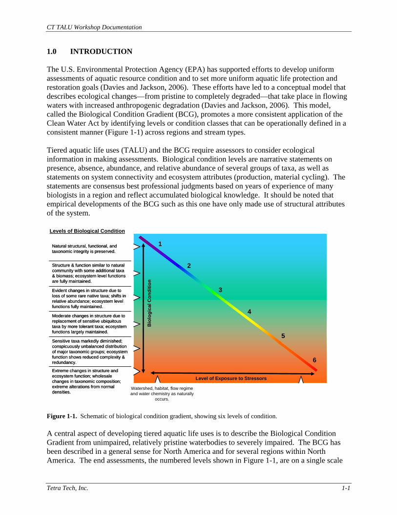
1.0 INTRODUCTION The U.S. Environmental Protection Agency (EPA) has supported efforts to develop uniform assessments of aquatic resource condition and to set more uniform aquatic life protection and restoration goals (Davies and Jackson, 2006). These efforts have led to a conceptual model that describes ecological changes—from pristine to completely degraded—that take place in flowing waters with increased anthropogenic degradation (Davies and Jackson, 2006). This model, called the Biological Condition Gradient (BCG), promotes a more consistent application of the Clean Water Act by identifying levels or condition classes that can be operationally defined in a consistent manner (Figure 1-1) across regions and stream types. Tiered aquatic life uses (TALU) and the BCG require assessors to consider ecological information in making assessments. Biological condition levels are narrative statements on presence, absence, abundance, and relative abundance of several groups of taxa, as well as statements on system connectivity and ecosystem attributes (production, material cycling). The statements are consensus best professional judgments based on years of experience of many biologists in a region and reflect accumulated biological knowledge. It should be noted that empirical developments of the BCG such as this one have only made use of structural attributes of the system.
Figure 1-1. Schematic of biological condition gradient, showing six levels of condition. A central aspect of developing tiered aquatic life uses is to describe the Biological Condition Gradient from unimpaired, relatively pristine waterbodies to severely impaired. The BCG has been described in a general sense for North America and for several regions within North America. The end assessments, the numbered levels shown in Figure 1-1, are on a single scale
Watershed, habitat, flow regime and water chemistry as naturally
occurs.
5
6
4
3
2
1
Levels of Biological Condition
Bio
logi
cal C
ondi
tion
Level of Exposure to Stressors Extreme changes in structure and ecosystem function; wholesale changes in taxonomic composition; extreme alterations from normal densities.
Sensitive taxa markedly diminished; conspicuously unbalanced distribution of major taxonomic groups; ecosystem function shows reduced complexity & redundancy.
Moderate changes in structure due to replacement of sensitive ubiquitous taxa by more tolerant taxa; ecosystem functions largely maintained.
Evident changes in structure due to loss of some rare native taxa; shifts in relative abundance; ecosystem level functions fully maintained.
Structure & function similar to natural community with some additional taxa & biomass; ecosystem level functions are fully maintained.
Natural structural, functional, and taxonomic integrity is preserved.
Extreme changes in structure and ecosystem function; wholesale changes in taxonomic composition; extreme alterations from normal densities.
Sensitive taxa markedly diminished; conspicuously unbalanced distribution of major taxonomic groups; ecosystem function shows reduced complexity & redundancy.
Moderate changes in structure due to replacement of sensitive ubiquitous taxa by more tolerant taxa; ecosystem functions largely maintained.
Evident changes in structure due to loss of some rare native taxa; shifts in relative abundance; ecosystem level functions fully maintained.
Structure & function similar to natural community with some additional taxa & biomass; ecosystem level functions are fully maintained.
Natural structural, functional, and taxonomic integrity is preserved.

CT TALU Workshop Documentation
Tetra Tech, Inc. 1-2
that can be applied nationwide. As a universal scale, the BCG can be calibrated to local conditions using specific, local expertise to apply it to conditions within a state. This report describes the application of the BCG to streams of Connecticut and the development of a more traditional multimetric index; either of which can be used for defining levels for restoration goals and aquatic life protection criteria. For clarity, we reiterate three important definitions: aquatic life use tiers, BCG levels, and BCG attributes. The tiers of the aquatic life use framework refer to programmatic categories of expected use attainment for waterbodies within a state. These should not be confused with the BCG levels, which are narrative descriptions of the biological condition with respect to a gradient from completely natural to severely disturbed. Unless specifically stated, we refer to levels of the BCG from this point forward. The BCG attributes are characteristics of the biological community, individual organisms within the community, and the physical environment. BCG attributes are used to help recognize BCG levels. The predominant BCG attributes used in this analysis are coded as numerals I through VI, which is the same range as the scale of the BCG levels, but level and attribute numbers are not identical or interchangeable. 1.1 The Biological Condition Gradient Stream communities change in response to pollution, and aquatic biologists have developed indexes to reflect and standardize these changes. Communities are altered on a relatively predictable gradient from pristine to slightly impaired to severely impaired. Indexes that reflect the gradient have included the Saprobien index (Cairns and Pratt, 1993), the index of biotic integrity (IBI; Karr et al., 1986), similarly constructed indexes for macroinvertebrates (Barbour et al., 1999), simple diversity and richness indexes that follow the general loss of native taxa with impairment (e.g., Cairns et al., 1993), and more complex indexes that compare observed taxa to model-predicted expected taxa, such as the River Invertebrate Prediction and Classification System (RIVPACS; Clarke et al., 1996). 1.1.1 Biological Attributes The BCG systematizes the cumulative knowledge of how aquatic communities change with disturbance by first identifying critical attributes of the community, and then by describing how each attribute changes in response to human disturbance. Through a series of national, EPA-sponsored workshops, a technical workgroup of State, Tribal, academic, and federal biologists described the BCG using the following 10 attributes (EPA, 2005; Davies and Jackson, 2006):
I. Historically documented, sensitive, long-lived or regionally endemic taxa: refers to taxa known to have been supported in a waterbody or region prior to enactment of the Clean Water Act, according to historical records compiled by state or federal agencies or published scientific literature. Sensitive or regionally endemic taxa have restricted, geographically isolated distribution patterns (occurring only in a locale as opposed to a region), often due to unique life history requirements. They may be long-lived, late maturing, low fecundity, limited mobility, or require a mutualist relation with other species. May be among listed endangered/threatened or special concern species. Predictability of occurrence is often low, therefore, requiring documented observation. Recorded occurrence may be highly dependent on sample methods, site selection and level of effort.
II. Highly Sensitive Taxa: taxa that naturally occur in low numbers relative to total population density
but may make up large relative proportion of richness. They may be ubiquitous in occurrence or
CT TALU Workshop Documentation
Tetra Tech, Inc. 1-3
may be restricted to certain micro-habitats, but because of low density, recorded occurrence is dependent on sample effort. Often stenothermic (having a narrow range of thermal tolerance) or cold-water obligates; they are commonly k-strategists (populations maintained at a fairly constant level; slower development; longer life-span). They may have specialized food resource needs or feeding strategies and are generally intolerant to significant alteration of the physical or chemical environment; is often the first taxa observed to be lost from a community.
III. Intermediate Sensitive Taxa, (or Sensitive and Common Taxa): taxa that are ordinarily common
and abundant in natural communities when conventional sample methods are used. They often have a broader range of thermal tolerance than Sensitive- Rare taxa. These are taxa that comprise a substantial portion of natural communities, and that often exhibit negative response (loss of population, richness) at mild pollution loads or habitat alteration.
IV. Taxa of Intermediate Tolerance: taxa that make up a substantial portion of natural communities;
may be r-strategists (early colonizers with rapid turn-over times; “boom/bust” population characteristics). They may be eurythermal (having a broad thermal tolerance range). May have generalist or facultative feeding strategies enabling utilization of relatively more diversified food types. Readily collected with conventional sample methods. May increase in number in waters with moderately increased organic resources and reduced competition but are intolerant of excessive pollution loads or habitat alteration.
V. Tolerant Taxa: Taxa that make up a low proportion of natural communities. These taxa often are
tolerant of a broader range of environmental conditions and are thus resistant to a variety of pollution or habitat induced stress. They may increase in number (sometimes greatly) in the absence of competition. Commonly r-strategists (early colonizers with rapid turn-over times; “boom/bust” population characteristics), able to capitalize when stress conditions occur. These are the last survivors in severely disturbed systems.
VI. Non-native or Intentionally Introduced Species: with respect to a particular ecosystem, any species
that is not found in that ecosystem. Species introduced or spread from one region of the U.S. to another outside their normal range are non-native or non-indigenous, as are species introduced from other continents.
VII. Organism Condition (especially of long-lived organisms): general indicators of organism health,
such as deformities, anomalies, lesions, tumors, or excess parasitism are all external indicators of condition.
VIII. Ecosystem Function: function includes trophic levels, production, respiration, total biomass and
biomass in functional levels, P/R ratios, etc.
IX. Spatial and Temporal Extent of Detrimental Effects: the spatial extent of damage or degradation from a particular source.
X. Ecosystem Connectance: natural connections and relation among ecosystem units, such as extent
fragmentation, connections of riparian areas with the stream and floodplain, etc. The last three attributes, Ecosystem Function, Spatial and Temporal Extent, and Ecosystem Connectance, were all deemed ecologically important by the workgroups that developed the BCG (Davies and Jackson, 2006), but none have been applied or tested in either regional or state contexts. There is disagreement among ecologists whether measures of ecosystem function provide unique information on condition not already provided by the more common structural measures. Attributes IX and X, both spatial attributes, were considered by some ecologists to be measures of stress, and not biological response to stress. Routine monitoring programs (including Connecticut’s) do not normally collect information on these attributes (VIII to X). In

CT TALU Workshop Documentation
Tetra Tech, Inc. 1-4
this development for Connecticut, we did not use attributes VII to X. Attribute VII, Organism Condition, is commonly measured by agencies that monitor fish and edible shellfish. 1.1.2 Levels of the Condition Gradient At the national workshops, biologists agreed that in most stream ecosystems it was possible to discriminate six levels in the condition gradient, ranging from undisturbed natural condition to severely degraded and almost devoid of natural life. The levels are described in terms of changes in the structure and function of native aquatic communities. Although the condition levels are described in terms of both structure and function, empirical application of the BCG have so far not incorporated the functional or spatial attributes.
1. Natural or native condition: Native structural, functional and taxonomic integrity is preserved; ecosystem function is preserved within the range of natural variability.
2. Minimal changes in structure of the biotic community and minimal changes in ecosystem
function: Virtually all native taxa are maintained with some changes in biomass and/or abundance; ecosystem functions are fully maintained within the range of natural variability.
3. Evident changes in structure of the biotic community and minimal changes in ecosystem
function: Evident changes in structure due to loss of some rare native taxa; shifts in relative abundance of taxa but sensitive-ubiquitous taxa are common and abundant; ecosystem functions are fully maintained through redundant attributes of the system.
. 4. Moderate changes in structure of the biotic community with minimal changes in
ecosystem function: Moderate changes in structure due to replacement of some sensitive-ubiquitous taxa by more tolerant taxa, but reproducing populations of some sensitive taxa are maintained; overall balanced distribution of all expected major groups; ecosystem functions largely maintained through redundant attributes.
5. Major changes in structure of the biotic community and moderate changes in ecosystem
function: Sensitive taxa are markedly diminished; conspicuously unbalanced distribution of major groups from that expected; organism condition shows signs of physiological stress; ecosystem function shows reduced complexity and redundancy; increased build-up or export of unused materials.
6. Severe changes in structure of the biotic community and major loss of ecosystem
function: Extreme changes in structure; wholesale changes in taxonomic composition; extreme alterations from normal densities and distributions; organism condition is often poor; ecosystem functions are severely altered.
1.2 Development of Attributes and Gradient for Connecticut Aquatic biologists familiar with Connecticut streams convened in a workshop to develop both the ecological attributes and rules for assigning sites to levels in the gradient. Their expertise included aquatic ecology, benthic macroinvertebrate sampling and monitoring, water quality, and
CT TALU Workshop Documentation
Tetra Tech, Inc. 1-5
fisheries biology. Although the BCG is intended to be developed and applied for as many taxonomic groups as possible (e.g., benthic macroinvertebrates, periphyton, fish, herpetofauna, vascular plants, etc.), this development of the gradient included systematic application to benthic macroinvertebrates only, collected by the methods used in Connecticut’s monitoring program. Integration of fish and other taxonomic groups into the descriptions of the BCG must await future iterations of the process. As in other applications, we developed the BCG using only Attributes I–VI, because the monitoring program does not collect information on the other attributes. After reviewing EPA’s conceptual model of the biological condition gradient, the group reviewed the list of taxa identified in the Connecticut ambient monitoring program to assign taxa to attribute groups I–VI. Appendix A includes the taxa list and assigned attribute groups. The group then considered data from selected monitoring sites and assigned the sites to levels in the BCG based on the taxa present in the sample. Details of these processes are presented in the Methods section. 1.3 Aquatic Life Uses A biological condition gradient requires strong scientific knowledge on the response of aquatic biological assemblages to stressors, as well as the biota inhabiting a region. Using the scientific information to better assess and manage living aquatic resources also requires a legal foundation that permits the determination of scientifically defensible management goals (policies, designated uses, standards, criteria) in keeping with the goals of the Clean Water Act. Finally, developing a quantitative methodology for assessing waterbodies in relation to the BCG requires a scientifically sound biological monitoring program. Under the Clean Water Act a state can identify use classes, called Designated Uses, for its waterbodies. As biological condition can be divided into levels, so can designated aquatic life uses of waterbodies be divided into tiers corresponding to the biological expectation for the different uses. The relationship between aquatic life use (ALU) tiers and BCG levels must be addressed in the context of State programs and policies. BCG development may be required for each tier of ALU (where the ALU tier is defined by environmental classification), or BCG levels may coincide with aquatic life use tiers (where the expected biological condition is the basis for the ALU tier). In this report, we focus on the BCG level development.
CT TALU Workshop Documentation
Tetra Tech, Inc. 2-1
2.0 METHODS The calibration process includes
• assessment of the state's biological monitoring program to support quantitative calibration of a regional BCG;
• identification of attributes of condition that will be used to build the BCG; assigning taxa to the attributes;
• development of the regional model of the BCG, and its calibration for operational assessment; and
• analysis of biological condition using additional tools to confirm BCG model development and to aid in its application.
The development process is iterative and may require several passes through the process to converge on a coherent, locally calibrated BCG that is scientifically defensible. 2.1 Connecticut Ambient Monitoring Program Consistent, high quality biological monitoring information is key to developing a quantitative assessment system within a BCG framework. Connecticut DEP operates a sizable ambient monitoring program throughout the state (CT DEP, 2005). The following description is excerpted from DEP’s draft report (CT DEP, 2004) “Ambient Water Quality Monitoring: Rotating Basin Approach Data Summary (1996–2001)”:
Connecticut contains a total of approximately 5,830 miles of rivers and streams (EPA, 1993). The Connecticut DEP has organized the hydrography of the State into a hierarchical system of natural drainage basins comprised of four basic levels of magnitude (CT DEP, 1981). Major basins represent the greatest level of magnitude and are roughly equivalent, but not identical to, USGS eight digit cataloging units. Major basins are comprised of three categories of sub basins; in order of decreasing magnitude, these are regional, sub-regional, and local basins. The distribution of drainage basin units at each level of magnitude is listed below. Beginning in 1996, the Bureau of Water Management (BWM) initiated a rotating basin approach to monitoring and assessment. This approach is consistent with the current 305(b) guidelines and the overall goal of a more comprehensive statewide assessment by ultimately increasing the number of river miles monitored. To accomplish this plan the State was divided into five hydrologic assessment units comprised of one or two CT DEP major basins, or USGS cataloging units. The assessment units are… shown in Figure 2-1. Monitoring and assessment efforts will be concentrated on one unit each year for a five-year period. Implementation began during the fall of 1996.
Sample Collection: The primary collection method follows EPA Rapid Bioassessment Protocol III (RBP III) for Streams and Rivers (Plafkin, 1989). RBP III involves collecting 12 kick samples (stops) throughout riffles at sampling sites using a rectangular net (18"x18"x10") with 800 × 900 µm mesh. The stops are spread out as best as possible both up, down, and across the riffle. The resulting sample is meant to represent the community as a whole within the riffle. The contents from all 12 stops are composited into sample container(s) and preserved in the field with 70% ethyl alcohol. An alternate method when

CT TALU Workshop Documentation
Tetra Tech, Inc. 2-2
habitat may be limited to the benthic community is RBP I (Plafkin et al., 1989). The primary difference with RBP III is that the organisms are removed directly from the debris in the net and are not sub-sampled in the laboratory under controlled conditions. Samples collected using the RBP I method are termed "NQ-Pick", for Non-quantitative Pick. Benthic community sites for each basin are sampled during the fall benthic community index period (October 1–November 30). Benthic community sampling can also occur during a spring index period (April 1–May 31), but based on experience, DEP considers the fall index period to better represent the worst-case condition. Since differences in habitat conditions are minimized with this approach, differences in the benthic communities of two sites should be primarily due to water quality differences. A complete description of sampling protocol is available in the Ambient Biological Monitoring-Benthic Macroinvertebrates Quality Assurance Project Plan (CT DEP, 2003b).
Laboratory Analysis: Identification is to lowest practical taxa based on a 200-organism minimum sub-sample. Based on the organisms present in the sub-sample, a series of community structure metrics are calculated and compared to metrics a reference site. A reference site is a specific locality on a waterbody that is minimally impaired and is representative of the expected ecological integrity of other localities on the same waterbody or nearby waterbodies. The final result of RBP III is an assessment of the impairment level of the benthic community. Rotating Secondary Physical/Chemical Monitoring Network This network is intended to supplement the primary network sites by providing physical/chemical data on selected rivers. Sampling frequency is quarterly for one year, which is consistent with the rotating basin schedule. Third quarter sampling events are coincident with critical stress periods characterized by low stream flow and elevated water temperature. Sampling site selection is based on a targeted approach considering sub basin size, location of wastewater discharges, land use, and resource value. Conventional water quality parameters, toxic metals, and indicator bacteria are measured by means of grab samples. Personnel from the DEP, Bureau of Water Management, perform sample collection and field measurements. The Connecticut Department of Public Health (CT DPH), Laboratory Division, conducted laboratory analyses (CT DEP, 2004).
Land Use/ Land Cover data Land cover data were obtained from the University of Connecticut’s Center for Land use Education and Research (CLEAR); (http://clear.uconn.edu/projects/landscape/index.htm). We used land cover estimated for 2002, in the following categories:
• Impervious surface • Developed land (built-up, roads) • Turf and grass (e.g., lawns and parks) • Agriculture and grass (e.g., pasture) • Deciduous forest • Coniferous forest • Water • Forested wetland • Non-forested freshwater wetland • Tidal wetland • Utility right-of-way • Barren land

CT TALU Workshop Documentation
Tetra Tech, Inc. 2-3
Connecticut DEP had delineated catchments for each sampling site in the data base and calculated the area of each land cover category within the catchment. Because the CLEAR database did not extend beyond Connecticut’s borders, some sites with catchments partially in Massachusetts and New York had incomplete land cover data. For data analysis, the two forest, water, and three wetland categories were added to define a “natural land cover” category. Data Management Currently, all benthic data and associated metadata are entered into a Microsoft Access database, where metrics and summary information are generated through queries. Some of the benthic data is still brought into Access through Excel sheets, but CT DEP is working towards entering all of the benthic data from the taxonomist’s logbook directly into Access via existing entry forms (M. Beauchene, pers. comm. to J. Gerritsen).
#Y
#Y
#Y
#Y#Y
#Y#Y
#Y
#Y
#Y
#Y
#Y
#Y
#Y
#Y
#Y#Y#Y
#Y
#Y#Y#Y
#Y
#Y#Y
#Y
#Y
#Y#Y#Y
#Y#Y
#Y#Y
#Y
#Y#Y#Y #Y
#Y
#Y
#Y
#Y
#Y
#Y
#Y
#Y #Y
#Y
#Y
#Y#Y
#Y
#Y
#Y
#Y
#Y
#Y#Y
#Y
#Y
#Y
#Y
#Y
#Y
#Y#Y
#Y
#Y
#Y
#Y
#Y
#Y
#Y
#Y
#Y
#Y
#Y#Y
#Y#Y
#Y
#Y
#Y#Y
#Y#Y
#Y#Y
#Y
#Y #Y #Y#Y
#Y
#Y
#Y
#Y
#Y
#Y
#Y
#Y
#Y
#Y
#Y#Y
#Y
#Y
#Y
#Y
#Y
#Y #Y#Y
#Y#Y#Y
#Y
#Y
#Y #Y
#Y
#Y
#Y
#Y#Y
#Y
#Y#Y
#Y
#Y
#Y#Y
#Y
#Y
#Y
#Y#Y#Y
#Y#Y#Y
#Y
#Y
#Y
#Y#Y#Y
#Y#Y#Y
#Y
#Y#Y
#Y #Y
#Y
#Y#Y
#Y
#Y#Y
#Y #Y
#Y
#Y
#Y#Y
#Y
#Y#Y
#Y
#Y#Y
#Y
#Y#Y
#Y #Y
#Y
#Y#Y
#Y
#Y
#Y
#Y
#Y
#Y#Y
#Y
#Y
#Y
#Y
#Y
#Y
#Y
#Y
#Y
#Y
#Y
#Y
#Y
#Y#Y
#Y#Y
#Y
#Y
#Y
#Y
#Y
#Y#Y
#Y
#Y#Y
#Y
#Y
#Y
#Y
#Y
#Y
#Y#Y
#Y
#Y
#Y
#Y
#Y
#Y
#Y
#Y
#Y
#Y
#Y
#Y
#Y
Macroinvertebrate Collection LocationsN = 227
Major BasinPawcatuckSE CoastalThamesConnecticutS. Central CoastalHousatonicSW CoastalHudson
#Y ABM Sample Location
Figure 2-1. Distribution of sampling sites across Connecticut as of 2001, showing major basins (from CT DEP, 2004).
CT TALU Workshop Documentation
Tetra Tech, Inc. 2-4
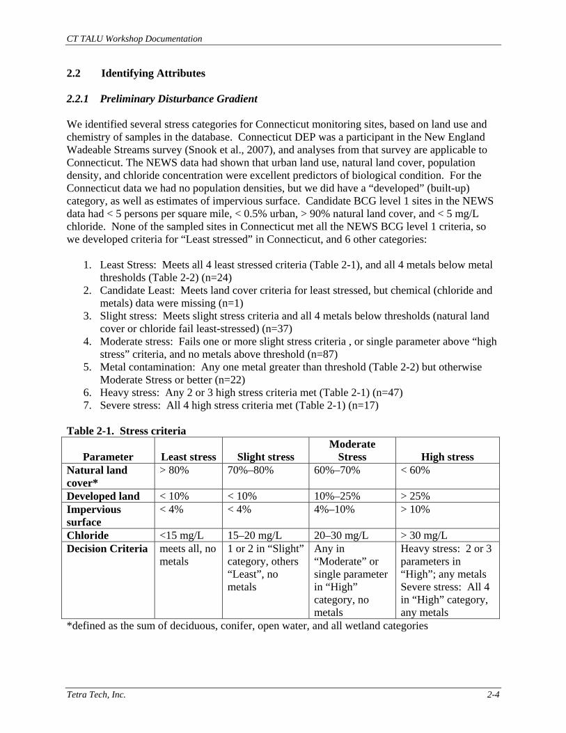
2.2 Identifying Attributes 2.2.1 Preliminary Disturbance Gradient We identified several stress categories for Connecticut monitoring sites, based on land use and chemistry of samples in the database. Connecticut DEP was a participant in the New England Wadeable Streams survey (Snook et al., 2007), and analyses from that survey are applicable to Connecticut. The NEWS data had shown that urban land use, natural land cover, population density, and chloride concentration were excellent predictors of biological condition. For the Connecticut data we had no population densities, but we did have a “developed” (built-up) category, as well as estimates of impervious surface. Candidate BCG level 1 sites in the NEWS data had < 5 persons per square mile, < 0.5% urban, > 90% natural land cover, and < 5 mg/L chloride. None of the sampled sites in Connecticut met all the NEWS BCG level 1 criteria, so we developed criteria for “Least stressed” in Connecticut, and 6 other categories:
1. Least Stress: Meets all 4 least stressed criteria (Table 2-1), and all 4 metals below metal thresholds (Table 2-2) (n=24)
2. Candidate Least: Meets land cover criteria for least stressed, but chemical (chloride and metals) data were missing (n=1)
3. Slight stress: Meets slight stress criteria and all 4 metals below thresholds (natural land cover or chloride fail least-stressed) (n=37)
4. Moderate stress: Fails one or more slight stress criteria , or single parameter above “high stress” criteria, and no metals above threshold (n=87)
5. Metal contamination: Any one metal greater than threshold (Table 2-2) but otherwise Moderate Stress or better (n=22)
6. Heavy stress: Any 2 or 3 high stress criteria met (Table 2-1) (n=47) 7. Severe stress: All 4 high stress criteria met (Table 2-1) (n=17)
Table 2-1. Stress criteria
Parameter Least stress Slight stress Moderate
Stress High stress Natural land cover*
> 80% 70%–80% 60%–70% < 60%
Developed land < 10% < 10% 10%–25% > 25% Impervious surface
< 4% < 4% 4%–10% > 10%
Chloride <15 mg/L 15–20 mg/L 20–30 mg/L > 30 mg/L Decision Criteria meets all, no
metals 1 or 2 in “Slight” category, others “Least”, no metals
Any in “Moderate” or single parameter in “High” category, no metals
Heavy stress: 2 or 3 parameters in “High”; any metals Severe stress: All 4 in “High” category, any metals
*defined as the sum of deciduous, conifer, open water, and all wetland categories

CT TALU Workshop Documentation
Tetra Tech, Inc. 2-5
Table 2-2. Metals Criteria (all dissolved) Metal Threshold (mg/L) notes Copper 0.008 Highest concentrations all impaired Iron 0.4 Effect marginal Nickel 0.01 Highest concentrations showed effects, but confounded
by detection limit Zinc 0.02 Strong effect Screening thresholds for metals (Table 2-2) were determined from scatterplots of number of mayfly or stonefly taxa in the samples vs. metal concentrations (Figure 2-2). These two orders are generally considered highly sensitive to metal contamination, in part due to the large number of chloride cells on their surfaces (e.g., Buchwalter and Luoma, 2005). Metals not included in Table 2-2 (Al, Cd, Hg, Pb, Se) were not associated with biological responses (Al, Hg, Pb), or had too few detectable observations in the data (Cd, Se). Data were not stratified for several other potential stressors (nutrients, BOD, total solids, coliform) because they were redundant with the stressor gradient classes described above. Using the criteria of Tables 2-1 and 2-2, we identified 24 Least Stressed sites as potential reference sites, and 17 Severely Stressed sites to help calibrate the BCG and the MMI (Table 2-3).
Figure 2-2. Number of Plecoptera (stonefly) taxa and dissolved copper concentration. The screening criterion was determined from sharp decline of stonefly taxa above 0.008 mg/L copper.
Least stressed Highly stressed Other
0.000 0.005 0.010 0.015 0.020 0.025 0.030
Copper, Dissolved (mg/L)
-1
0
1
2
3
4
5
6
7
8
9
Ple
copt
era
Taxa
Screening criterion
CT TALU Workshop Documentation
Tetra Tech, Inc. 2-6
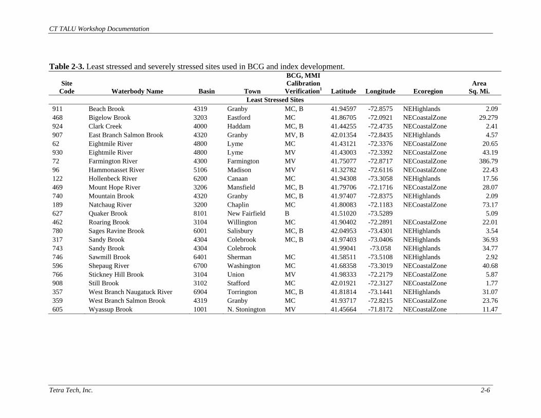
Table 2-3. Least stressed and severely stressed sites used in BCG and index development.
Site Code Waterbody Name Basin Town
BCG, MMI Calibration Verification1 Latitude Longitude Ecoregion
Area Sq. Mi.
Least Stressed Sites 911 Beach Brook 4319 Granby MC, B 41.94597 -72.8575 NEHighlands 2.09 468 Bigelow Brook 3203 Eastford MC 41.86705 -72.0921 NECoastalZone 29.279 924 Clark Creek 4000 Haddam MC, B 41.44255 -72.4735 NECoastalZone 2.41 907 East Branch Salmon Brook 4320 Granby MV, B 42.01354 -72.8435 NEHighlands 4.57 62 Eightmile River 4800 Lyme MC 41.43121 -72.3376 NECoastalZone 20.65 930 Eightmile River 4800 Lyme MV 41.43003 -72.3392 NECoastalZone 43.19 72 Farmington River 4300 Farmington MV 41.75077 -72.8717 NECoastalZone 386.79 96 Hammonasset River 5106 Madison MV 41.32782 -72.6116 NECoastalZone 22.43 122 Hollenbeck River 6200 Canaan MC 41.94308 -73.3058 NEHighlands 17.56 469 Mount Hope River 3206 Mansfield MC, B 41.79706 -72.1716 NECoastalZone 28.07 740 Mountain Brook 4320 Granby MC, B 41.97407 -72.8375 NEHighlands 2.09 189 Natchaug River 3200 Chaplin MC 41.80083 -72.1183 NECoastalZone 73.17 627 Quaker Brook 8101 New Fairfield B 41.51020 -73.5289 5.09 462 Roaring Brook 3104 Willington MC 41.90402 -72.2891 NECoastalZone 22.01 780 Sages Ravine Brook 6001 Salisbury MC, B 42.04953 -73.4301 NEHighlands 3.54 317 Sandy Brook 4304 Colebrook MC, B 41.97403 -73.0406 NEHighlands 36.93 743 Sandy Brook 4304 Colebrook 41.99041 -73.058 NEHighlands 34.77 746 Sawmill Brook 6401 Sherman MC 41.58511 -73.5108 NEHighlands 2.92 596 Shepaug River 6700 Washington MC 41.68358 -73.3019 NECoastalZone 40.68 766 Stickney Hill Brook 3104 Union MV 41.98333 -72.2179 NECoastalZone 5.87 908 Still Brook 3102 Stafford MC 42.01921 -72.3127 NECoastalZone 1.77 357 West Branch Naugatuck River 6904 Torrington MC, B 41.81814 -73.1441 NEHighlands 31.07 359 West Branch Salmon Brook 4319 Granby MC 41.93717 -72.8215 NECoastalZone 23.76 605 Wyassup Brook 1001 N. Stonington MV 41.45664 -71.8172 NECoastalZone 11.47

CT TALU Workshop Documentation
Tetra Tech, Inc. 2-7
Table 2-3. Continued. Site
Code Waterbody Name Basin Town BCG, MMI Calibration Verification1
Latitude Longitude Ecoregion Area Sq. Mi.
Severely Stressed Sites 76 Five Mile River 7401 New Canaan MC 41.14183 -73.4833 NECoastalZone 6.23 119 Hockanum River 4500 Manchester MC 41.78828 -72.5503 NECoastalZone 55.48 110 Hockanum River 4500 East Hartford MV 41.78218 -72.5912 NECoastalZone 74.40 159 Mad River 6914 Waterbury MC, B 41.54393 -73.0384 NECoastalZone 25.93 233 Noroton River 7403 Stamford MC, B 41.08984 -73.5152 NECoastalZone 9.58 236 Norwalk River 7300 Norwalk MC, B 41.13587 -73.426 NECoastalZone 27.61 267 Pequabuck River 4315 Bristol MC, B 41.67381 -72.8977 NECoastalZone 45.64 269 Pequonnock River 7105 Trumbull MC 41.2343 -73.1838 NECoastalZone 22.08 272 Piper Brook 4402 Newington MC 41.71861 -72.7274 NECoastalZone 17.21 289 Quinnipiac River 5200 Wallingford MC, B 41.45008 -72.8407 NECoastalZone 110.98 514 Steele Brook 6912 Waterbury 41.56869 -73.0574 NECoastalZone 17.04 331 Steele Brook 6912 Waterbury MV 41.58051 -73.0703 NECoastalZone 17.04 339 Still River 6600 Danbury MC 41.40633 -73.4253 NECoastalZone 38.05 333 Still River 6600 Brookfield MC, B 41.4389 -73.401 NECoastalZone 52.33 338 Still River 6600 Danbury MV 41.38981 -73.4637 NECoastalZone 14.43 342 Sympaug Brook 6604 Danbury MC, B 41.39229 -73.4284 NECoastalZone 7.25 354 Trout Brook 4403 West Hartford MV 41.73135 -72.7231 NECoastalZone 17.75
1 MC: MMI calibration site; MV: MMI verification site; B: BCG panel calibration site; Blank: Not used for calibration - met criteria for reference or stressed but too close to another site used in index development; would have represented redundant data.

CT TALU Workshop Documentation
Tetra Tech, Inc. 2-8
2.2.2 Taxa List and Site Gradient Prior to calibrating BCG levels, the workgroup assigned Connecticut taxa to the taxonomic attribute groups (Attributes I to VI; Section 1.1.1). Assignments of taxa to attributes relied on a combination of empirical examination of taxon occurrences at sites in the different stress classes, as well as professional experience of field biologists who had sampled the streams of Connecticut. The empirical analyses and professional opinions tended to agree, but in cases of disagreement, the group relied on consensus professional opinion, unless contradicted by an overwhelming response in the data analysis. As a group, participants discussed each taxon in the calibration data set, and developed a consensus assignment (Appendix A). Biologists have long observed that taxa differ in their sensitivity to pollution and disturbance. While biologists largely agree on the relative sensitivity of taxa, there may be subtle differences among stream types (high vs. low gradient) or among geographic regions. The workgroup empirically examined the sensitivities of the benthic macroinvertebrates to the generalized stressor gradient classes described above. 2.3 Development of the BCG Calibrating a regional BCG requires adjustment of the generalized conceptual model to regional conditions (Davies and Jackson, 2006; EPA, 2005; summarized in the Introduction). This includes components that construct a coherent ecological description of response to stressors in keeping with ecological theory and empirical observation: • Describe the native aquatic assemblages under natural, undisturbed conditions. The
description of natural conditions requires biological knowledge of the region, a natural classification of the assemblages, and, if available, historical descriptions of the habitats and assemblages.
• Identify regional stressors. A description of regionally dominant stressors will help define expectations for biological responses that are likely to occur. This step considers sources of physical and chemical stressors and causes of land use disturbance.
• Quantitative description of BCG levels that are the system responses to anthropogenic stressors.
2.3.1 Classification Bioassessment is based on developing expectations for natural conditions where there are many natural variables (such as stream size, slope, dominant natural substrate, etc.) which may affect species composition of undisturbed streams. Accordingly, a critical step in any bioassessment development is to classify the natural conditions to the extent that they affect the biological indicators (Gerritsen and Paul, 2006). Strata of biologically similar groups can be identified among reference sites through examination of biological gradients or assemblage types and association of the biological gradient with natural variables. We used non-metric multidimensional scaling (NMS) of the taxonomic data to
CT TALU Workshop Documentation
Tetra Tech, Inc. 2-9
examine potential groupings. Additional supporting analyses included indicator species analysis, correlations, cluster analysis, metric distribution plots, and regression analysis. Stratification into distinct site classes is useful when each of the resulting classes is represented by sufficient numbers of samples to allow meaningful analysis within or among site classes. NMS allows a comparison of taxa within each sample and an arrangement of the samples so that similar samples plot closer together than dissimilar samples in multiple dimensions. Natural environmental variables can be associated with the biological gradient through correlations with the biologically defined axes of the NMS diagram. NMS is a robust method for detecting similarity and differences among ecological community samples and works as well using presence/absence data as relative abundance data (McCune and Grace, 2002). A site by taxa matrix was compiled. Similarity among reference biological samples was made using the Bray-Curtis (BC) similarity measure. The BC formula is sometimes written in shorthand as
BC = 1-2W/(A+B)
where W is the sum of shared abundances and A and B are the sums of abundances in individual sample units. The ordination software (PC-Ord, McCune and Grace, 2002) calculates a site by site matrix of BC similarity from which the arrangement of samples in the ordination diagram is derived. Multiple dimensions are compressed into two or three dimensions that we can perceive. Rare and ambiguous taxa are not useful in the NMS ordination. Rare taxa were defined as those that occurred in less than three reference samples. Ambiguous taxa are those that are identified at higher taxonomic levels because of damaged or undeveloped specimens. The site by taxa matrix was therefore reduced to retain as much information as possible while excluding rare and ambiguous taxa. When several rare genera occurred within one family or when several identifications were at the family level, then all individuals were counted at the family level. When most identifications within a family were made at genus level, then the fewer identifications made at family level were excluded from the analysis. The site by environmental variable matrix included location information and catchment characteristics. The NMS ordination methods used in classification of natural strata were also used in distinguishing taxa responses to the stressor gradient. 2.3.2 BCG levels BCG level descriptions in the conceptual model tend to be rather general (e.g., “reduced richness”). To allow for consistent assignments of sites to BCG levels, it is necessary to operationalize, or codify, the general BCG level descriptions into a set of rules that anyone can follow and obtain the same BCG level assignments as the group of experts. Operational rules codify the BCG level descriptions (“as naturally occur”, “reduced”, “greatly reduced”, etc.) to quantitative or semi-quantitative rules for each attribute (“Attribute 2 taxa > 50% of any other attribute”). These rules preserve the collective professional judgment of the

CT TALU Workshop Documentation
Tetra Tech, Inc. 2-10
expert group and set the stage for the development of models that reliably assign sites to BCG levels without having to reconvene the same group. In essence, the rules and the models capture the group’s collective decision criteria. Rules are logic statements that experts use to make their decisions, for example: “If taxon richness is high, then biological condition is high.” Rules on attributes can be combined, for example: “If the number of highly sensitive taxa (Attribute II) is high, and the number of tolerant individuals (Attribute V) is low, then the BCG level is 2.” In questioning individuals on how decisions are made in assigning sites to BCG levels, it became evident that rules are not sharply defined (“crisp”). For example, there is no distinct number of highly sensitive taxa that would always distinguish BCG level 2 from BCG level 3. Rather, people use strength of evidence in allowing some deviation from their ideal for any individual attributes, as long as most attributes are in or near the desired range. Clearly, the definitions of “high,” “moderate,” “low,” etc., are uncertain. These rules preserve the collective professional judgment of the expert group and set the stage for the development of models that reliably assign sites to BCG levels without having to reconvene the same group. In essence, the rules and the models capture the group’s collective decision criteria. Rule development required discussion and documentation of BCG level assignment decisions and the reasoning behind the decisions. During this discussion, we recorded
• each participant’s decision (“vote”) for the site;
• the critical or most important information for the decision—for example, the number of taxa of a certain attribute, the abundance of an attribute, the presence of indicator taxa, etc.; and
• any confounding or conflicting information and how this was resolved for the eventual decision.
Rule development was iterative. Following the initial development phase, the draft rules were tested by the panel to ensure that new data and new sites are assessed in the same way. The test sites had not been used in the initial rule development and also spanned the range of anthropogenic stress. Any remaining ambiguities and inconsistencies from the first iterations were also resolved. Rules can be used directly for assessments, for calibrating other assessment methods (e.g., multimetric index or discriminant model), or as the basis of an expert system. 2.4 Decision Criteria Model Consensus professional judgment used to describe the BCG levels can take into account nonlinear responses, uncommon stressors, masking of responses, and unequal weighting of attributes. This is in contrast to the commonly used biological indexes, which are typically unweighted sums of attributes (e.g., multimetric indexes; Karr and Chu, 1999; Barbour et al., 1999), or a single attribute, observed to expected taxa (e.g., Wright, 2000; Simpson and Norris, 2000). Consensus assessments built from the professional judgment of many experts result in a high degree of confidence in the assessments, but the assessments are labor-intensive (several experts must rate each site). It is also not practical to reconvene the same group of experts for every site monitored in a long-term program for assessment and management. Since individuals
CT TALU Workshop Documentation
Tetra Tech, Inc. 2-11
may be replaced on a panel over time, assessments may in turn “drift” due to individual differences of new panelists. Management and regulation, however, require clear and consistent methods and rules for assessment, which do not drift unless deliberately reset. Use of the BCG in operational monitoring, management, and regulation thus requires a way to automate the consensus expert judgment so that the assessments are consistent until such time that they are explicitly altered due to new knowledge becoming available. Two options have been used in the past: the Maine DEP developed a set of multivariate linear discriminant models to imitate the expert consensus and predict a site assessment (Davies et al., 1995); and the UK Environmental Agency defined ranges of scores of two indexes (their RIVPACS index and a tolerance index) that corresponded to the expert consensus (Hemsley-Flint, 2000). Both of these approaches require one or more multivariate statistical models to statistically predict the expert judgment in assessments. Instead of a statistical prediction of expert judgment, we have chosen to use a methodology that directly, explicitly and transparently converts the expert consensus to automated site assessment. The method uses fuzzy set theory applied to rules developed by the group of experts. Fuzzy sets and fuzzy logic are directly applicable to environmental assessment; they have been used extensively in engineering applications worldwide (e.g., Demicco and Klir, 2004) and environmental applications have been explored in Europe and Asia (e.g., Castella and Speight, 1996; Ibelings et al., 2003). We applied the approach for a fuzzy-set model developed for BCG assessment in New Jersey (Gerritsen et al., submitted), modified for the rules developed specifically for Connecticut streams. Fuzzy sets and fuzzy logic allow degrees of membership (in sets) and degrees of truth (in logic), compared to all-or-nothing in classical set theory and logic. This has immediate advantages in scientific classification, for example, “sand” and “gravel,” where a particle with diameter of 1.999 mm is classified as “sand” in classical set theory, and one with 2.001 mm diameter is classified as “gravel.” In fuzzy set theory, both particles may have nearly equal membership in both classes (Demicco, 2004). Demicco and Klir (2004) proposed four reasons why fuzzy sets and fuzzy logic enhance scientific methodology
• fuzzy sets can capture “irreducible measurement uncertainty”, as in the sand/gravel example above;
• fuzzy logic captures vagueness of linguistic terms, such as “many,” “large” or “few”; • fuzzy sets and logic can be used to manage complexity and computational costs of
control and decision systems; and • fuzzy logic enhances the ability to model human reasoning and decision-making.
2.5 Multimetric Index (MMI) Development MMIs incorporate several signals of biological response by combining multiple measurements of a sample. In this analysis, the MMI was used to confirm results of the BCG calibration and to provide another tool for its application. The premise of the index development process is that physical and chemical disturbances are reflected by changes in the benthic macroinvertebrate community. Physical and chemical characteristics can first be used to distinguish minimally

CT TALU Workshop Documentation
Tetra Tech, Inc. 2-12
disturbed (reference) sites from sites disturbed through human activity. Meaningful biological signals of disturbance are summarized in a multimetric index that can be used to evaluate biological integrity in sites of unknown quality. The development of a multimetric index calibrated on the benthic macroinvertebrate and environmental data collected in wadeable Connecticut streams followed a series of steps, as follows:
1. Collect and organize the data; 2. Define reference and stressed sites; 3. Stratify natural biological conditions; 4. Calculate biological metrics and determine metric sensitivity to stresses; 5. Combine appropriate metrics into index alternatives; 6. Select the most appropriate index for application in high gradient streams based on
sensitivity and variability, and; 7. Assess performance of the index.

CT TALU Workshop Documentation
Tetra Tech, Inc. 3-1
3.0 STREAMS AND BENTHOS OF CONNECTICUT-DESCRIPTIVE RESULTS 3.1 Regional Description Connecticut is similar to most of the rest of the eastern US in the historical patterns of settlement and land use. Initial clearing of native forest was primarily for agriculture, towns, and lumber needs in the Colonial and early Federal eras. By the late 1700s, most of the native forest had been clearly (Bell, 1985). Connecticut’s abundant water power from high gradient streams fostered early industrial development from the late Colonial era until the advent of steam power. Dominant industries of the 19th century were iron, copper, and textiles. The iron industry used local areas and charcoal for smelting, resulting in severe deforestation and firewood shortages in the mid-1800s (Bell, 1985). Connecticut’s iron industry disappeared by the early 20th century because it could not compete against Midwestern large-scale and steel mill. The copper industry and textiles remained important until the mid-20th century, after which they also declined. Light and medium industrial development continued through the middle of the 20th century, but the large-scale basic industries of steel and refining were limited by distance from raw materials. Industrialization also left a legacy on the landscape and in the state’s waterbodies, often as buried or exposed contamination, which may leach or run off into streams. Agriculture was more extensive in the uplands and hills outside of major river valleys prior to the US Civil War (1861-65) than it is today. The growth of railroad transportation during the 19th century led to the importation of cheaper food from the Midwest. Economically marginal farms established on rocky upland soils were largely abandoned in the period between 1870 and 1930, and reverted to forest (e.g., Bell, 1985). A legacy of 18th and 19th century agriculture is the stone fences now seen throughout New England’s forests. Connecticut has been urbanized since the peak of 19th century industrial development. Major urban areas today include the southwestern counties that form suburbs and exurbs of New York, New Haven and Hartford. Increasing suburban development extending from urban centers has led to extensive conversion of mixed agriculture and regrown wooded land to urban and suburban uses (e.g., Bell, 1985; Maizel et al., 1998). 3.2 Stream Classification Ordination In the NMS ordination of reference samples, the strongest classification variable was catchment size category. In ordinations of sites in taxa space (both presence/absence and relative abundance), the small and large sites (cutoff 10 square miles) are on opposite ends of the first axis (Figure 3-1). The smaller sites have more representation by the flies (Diptera), especially midges (Chironomidae). Mayflies, stoneflies, and caddisflies (Ephemeroptera, Plecoptera, and Trichoptera; EPT) were more dominant in larger sites (especially mayflies). Cluster analysis A cluster analysis revealed obvious groupings based on two or three clusters. With only two clusters, sample similarities based on relative abundance and on presence/absence give identical results. Discriminant function analysis (DFA) was used to identify natural determinants of the

CT TALU Workshop Documentation
Tetra Tech, Inc. 3-2
distinctive biological groupings. The DFA was efficient at identifying two clusters based on catchment size alone. After entering catchment size in the models, other variables (e.g., ecoregion, latitude, longitude) have insignificant discriminatory power. Ecoregion was coded as a binary variable (NE Coastal Zone = 0, NE Highlands = 1). Classification errors increased when models identifying three groups were attempted.
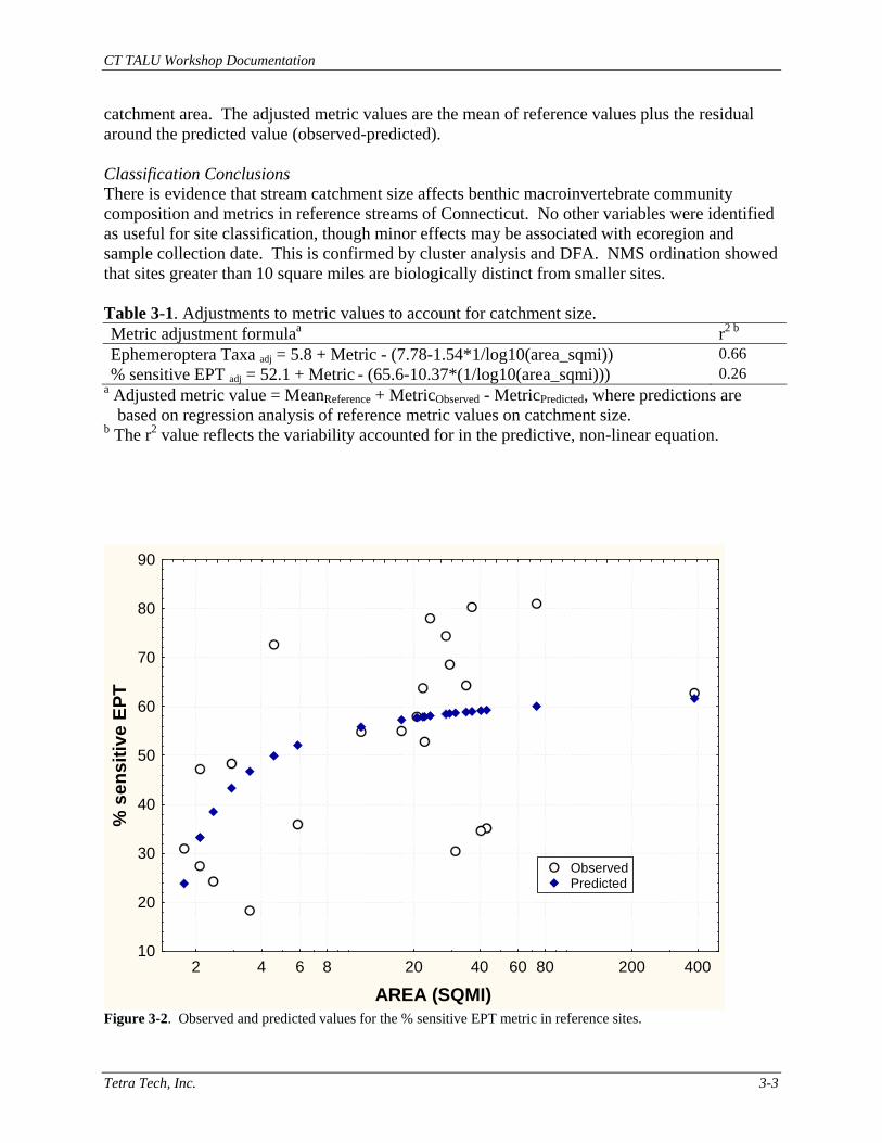
Figure 3-1. NMS ordination of reference data by presence/absence and relative abundance of benthic macroinvertebrates. Correlation and Regression Analysis Seventeen (17) reference metrics were significantly correlated with catchment area and two with ecoregion. Only two of the metrics that showed significant correlations with catchment area were considered in index development. The other metrics correlated with catchment area did not discriminate between reference and stressed sites. Small streams tend to have fewer mayfly taxa and a smaller proportion of sensitive EPT individuals than larger streams. Midges and Diptera (taxa and relative abundance of individuals) can be dominant in small reference streams (displacing the sensitive EPTs). The pattern described agrees with CT DEP biologist’s observations that small streams can be dominated by midges. Regression analysis was used to derive an adequate adjustment for the metrics so that differences in catchment size would not affect metric and index scoring (Table 3-1, Figures 3-2–3-3). Because of the asymptotic form of the relationship, a regression equation was fit in the form of b-m(1/x) where x is the log of
CT TALU Workshop Documentation
Tetra Tech, Inc. 3-3
catchment area. The adjusted metric values are the mean of reference values plus the residual around the predicted value (observed-predicted). Classification Conclusions There is evidence that stream catchment size affects benthic macroinvertebrate community composition and metrics in reference streams of Connecticut. No other variables were identified as useful for site classification, though minor effects may be associated with ecoregion and sample collection date. This is confirmed by cluster analysis and DFA. NMS ordination showed that sites greater than 10 square miles are biologically distinct from smaller sites. Table 3-1. Adjustments to metric values to account for catchment size. Metric adjustment formulaa r2 b Ephemeroptera Taxa adj = 5.8 + Metric - (7.78-1.54*1/log10(area_sqmi)) 0.66 % sensitive EPT adj = 52.1 + Metric - (65.6-10.37*(1/log10(area_sqmi))) 0.26
a Adjusted metric value = MeanReference + MetricObserved - MetricPredicted, where predictions are based on regression analysis of reference metric values on catchment size.
b The r2 value reflects the variability accounted for in the predictive, non-linear equation.
2 4 6 8 20 40 60 80 200 400
AREA (SQMI)
10
20
30
40
50
60
70
80
90
% s
ensi
tive
EPT
Observed Predicted
Figure 3-2. Observed and predicted values for the % sensitive EPT metric in reference sites.

CT TALU Workshop Documentation
Tetra Tech, Inc. 3-4
2 4 6 8 20 40 60 80 200 400
AREA (SQMI)
1
2
3
4
5
6
7
8
9Ep
hem
erop
tera
Tax
a
Observed Predicted
Figure 3-3. Observed and predicted values for the Ephemeroptera taxa metric in reference sites. Correlation analysis reveals that several metrics are related to catchment area. However, many of the correlated metrics are not the strongest indicators of environmental stress (see Section 6 below). Distinct site classification introduces an artificial “breakpoint” to define the different classes, such as, sites above, or below, 10 square miles in catchment area. However, a site that is 9 square miles may be very similar to a site that is 11 square miles. A continuous classification system adjusts individual metrics on a site specific basis, as demonstrated in the regression analysis. It is more appropriate than discrete classification in this analytical data set because: continuous classification avoids the artificial threshold between site categories, and it allows application of a single index in all sites, as opposed to applying different indices or different metric scoring scales depending on site class. The classification adjustments are applied only in the limited number of metrics that show effects of natural environmental gradients. It allows analysis of all data combined, which increases the robustness of the index development results compared to separate development processes for a smaller number of samples in each site class. 3.3 BCG Taxa Attributes Graphical analysis of individual taxa on ordination plots was deemed to be the most useful for identifying attribute groups. The response gradient was defined by ordination analysis, where the least stressed and the most stressed sites were identified in the ordination, and where the least and most stressed sites were well-separated in the ordination (Figure 3-4). These sites thus represent the endpoints of the stressor gradient in ordination space, and the stressor gradient was
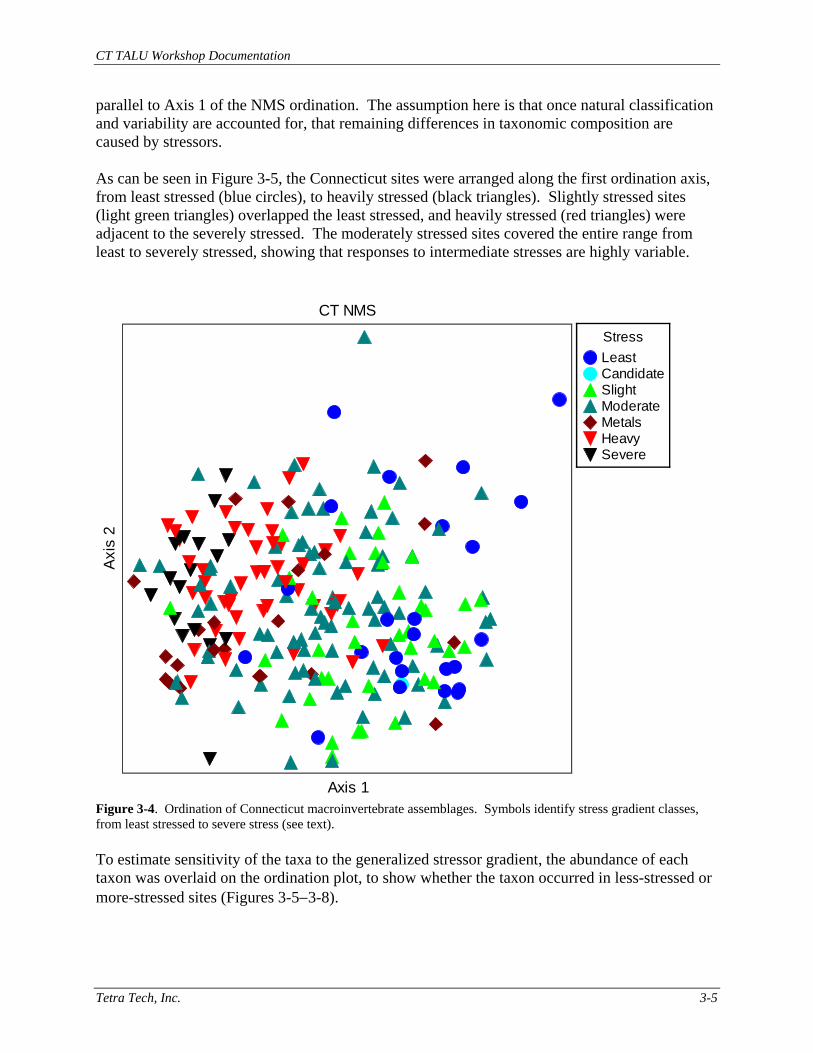
CT TALU Workshop Documentation
Tetra Tech, Inc. 3-5
parallel to Axis 1 of the NMS ordination. The assumption here is that once natural classification and variability are accounted for, that remaining differences in taxonomic composition are caused by stressors. As can be seen in Figure 3-5, the Connecticut sites were arranged along the first ordination axis, from least stressed (blue circles), to heavily stressed (black triangles). Slightly stressed sites (light green triangles) overlapped the least stressed, and heavily stressed (red triangles) were adjacent to the severely stressed. The moderately stressed sites covered the entire range from least to severely stressed, showing that responses to intermediate stresses are highly variable.
CT NMS
Axis 1
Axi
s 2
StressLeastCandidateSlightModerateMetalsHeavySevere
Figure 3-4. Ordination of Connecticut macroinvertebrate assemblages. Symbols identify stress gradient classes, from least stressed to severe stress (see text). To estimate sensitivity of the taxa to the generalized stressor gradient, the abundance of each taxon was overlaid on the ordination plot, to show whether the taxon occurred in less-stressed or more-stressed sites (Figures 3-5−3-8).
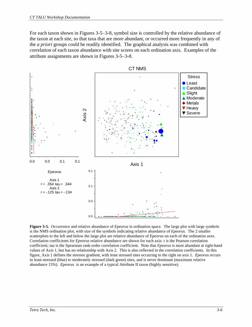
CT TALU Workshop Documentation
Tetra Tech, Inc. 3-6
For each taxon shown in Figures 3-5−3-8, symbol size is controlled by the relative abundance of the taxon at each site, so that taxa that are more abundant, or occurred more frequently in any of the a priori groups could be readily identified. The graphical analysis was combined with correlation of each taxon abundance with site scores on each ordination axis. Examples of the attribute assignments are shown in Figures 3-5−3-8.
CT NMS
Axis 1
Axi
s 2
0.0
0.0
0.1
0.1Epeorus
Axis 1r = .354 tau = .344
Axis 2r = -.125 tau = -.134
0.0 0.0 0.1 0.1
StressLeastCandidateSlightModerateMetalsHeavySevere
Figure 3-5. Occurrence and relative abundance of Epeorus in ordination space. The large plot with large symbols is the NMS ordination plot, with size of the symbols indicating relative abundance of Epeorus. The 2 smaller scatterplots to the left and below the large plot are relative abundance of Epeorus on each of the ordination axes. Correlation coefficients for Epeorus relative abundance are shown for each axis: r is the Pearson correlation coefficient; tau is the Spearman rank-order correlation coefficient. Note that Epeorus is most abundant at right-hand values of Axis 1, but has no relationship with Axis 2. This is also reflected in the correlation coefficients. In this figure, Axis 1 defines the stressor gradient, with least stressed sites occurring to the right on axis 1. Epeorus occurs in least-stressed (blue) to moderately stressed (dark green) sites, and is never dominant (maximum relative abundance 15%). Epeorus is an example of a typical Attribute II taxon (highly sensitive).
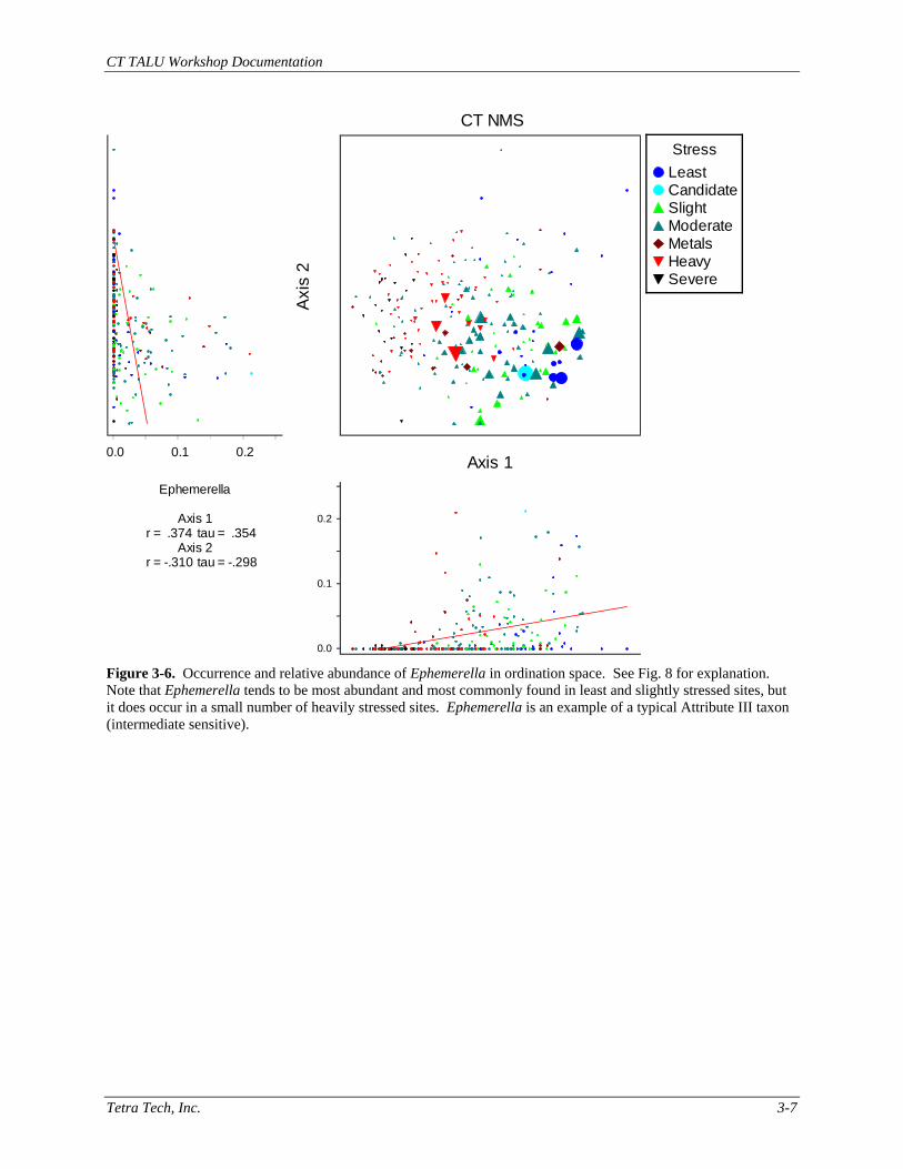
CT TALU Workshop Documentation
Tetra Tech, Inc. 3-7
CT NMS
Axis 1
Axi
s 2
0.0
0.1
0.2
Ephemerella
Axis 1r = .374 tau = .354
Axis 2r = -.310 tau = -.298
0.0 0.1 0.2
StressLeastCandidateSlightModerateMetalsHeavySevere
Figure 3-6. Occurrence and relative abundance of Ephemerella in ordination space. See Fig. 8 for explanation. Note that Ephemerella tends to be most abundant and most commonly found in least and slightly stressed sites, but it does occur in a small number of heavily stressed sites. Ephemerella is an example of a typical Attribute III taxon (intermediate sensitive).

CT TALU Workshop Documentation
Tetra Tech, Inc. 3-8
CT NMS
Axis 1
Axi
s 2
0
3.2E-02Corydalus
Axis 1r = .109 tau = .132
Axis 2r = -.210 tau = -.214
0 3.2E-02
StressLeastCandidateSlightModerateMetalsHeavySevere
Figure 3-7. Occurrence and relative abundance of Corydalus in ordination space. See Fig. 8 for explanation. Corydalus is most abundant in moderate stressed sites, but occurs in all stress categories from least-stressed to severe. Corydalus is an example of a typical Attribute IV taxon (intermediate-tolerant).

CT TALU Workshop Documentation
Tetra Tech, Inc. 3-9
CT NMS
Axis 1
Axi
s 2
0.0
0.4
0.8
Hydropsyche
Axis 1r = -.491 tau = -.397
Axis 2r = .486 tau = .405
0.0 0.4 0.8
StressLeastCandidateSlightModerateMetalsHeavySevere
Figure 3-8. Occurrence and relative abundance of Hydropsyche in ordination space. See Fig. 8 for explanation. Hydropsyche is most abundant in heavily stressed and severely-stressed sites, and is an example of a typical Attribute V taxon (tolerant). The genus occurs at reduced abundance, and reduced frequency, in least-stressed sites. Breakdown of taxa by attribute group is shown in Table 3-2. The Connecticut taxa list and final attribute assignments are given in Appendix A. Thirty six taxa were left unassigned because participants felt there was insufficient information on the taxa, or they were too rare in the dataset.
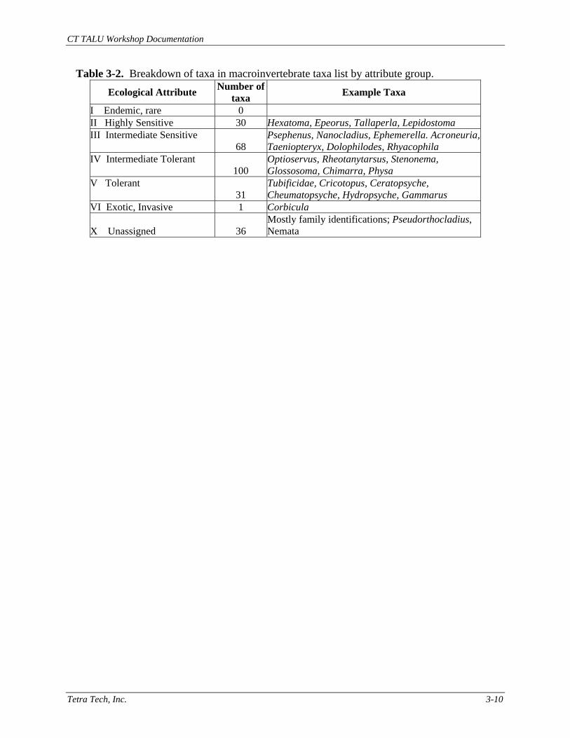
CT TALU Workshop Documentation
Tetra Tech, Inc. 3-10
Table 3-2. Breakdown of taxa in macroinvertebrate taxa list by attribute group.
Ecological Attribute Number of taxa Example Taxa
I Endemic, rare 0 II Highly Sensitive 30 Hexatoma, Epeorus, Tallaperla, Lepidostoma III Intermediate Sensitive 68
Psephenus, Nanocladius, Ephemerella. Acroneuria, Taeniopteryx, Dolophilodes, Rhyacophila
IV Intermediate Tolerant 100
Optioservus, Rheotanytarsus, Stenonema, Glossosoma, Chimarra, Physa
V Tolerant 31
Tubificidae, Cricotopus, Ceratopsyche, Cheumatopsyche, Hydropsyche, Gammarus
VI Exotic, Invasive 1 Corbicula
X Unassigned 36 Mostly family identifications; Pseudorthocladius, Nemata

CT TALU Workshop Documentation
Tetra Tech, Inc. 4-1
4.0 BIOLOGICAL CONDITION GRADIENT (BCG) 4.1 Site Assignments and BCG level Descriptions The workgroup examined macroinvertebrate data from 48 high gradient sites and was able to reach consensus on the BCG level assignments for all sites reviewed. Data for each site, notes and decisions are in Appendix B. In some cases, there was discussion and some disagreement on which of two adjacent BCG levels a site should be assigned to. These sites were apparently intermediate, with characteristics of both of the adjacent BCG levels. The group was able to distinguish 5 separate BCG levels (BCG levels 2-6). The first BCG level described in Davies and Jackson (2006) consists of entirely pristine sites, and was not included because there was no clear consensus whether BCG level 1 (pristine) sites actually occur in Connecticut. Nevertheless, two of the least stressed sites examined appeared to be candidates for BCG level 1 status. Further examination may be necessary to determine if these sites meet criteria for “minimally disturbed” (Stoddard et al., 2006). 4.2 Operational Rule Development Examinations of taxonomic attributes among the BCG levels determined by the panel showed that several of the attributes are useful in distinguishing levels, and indeed, were used by the panel’s biologists for decision criteria. Statistical summaries of each attribute and BCG level are given in Table 6, and are shown graphically in Figures 4-1 and 4-2. The group had developed preliminary decision rules for Connecticut data during the earlier NEWS data analysis (43 sites); however, the NEWS rules were calibrated to the NEWS multihabitat sampling methodology, and not to Connecticut’s riffle-only samples. Using the data distributions shown in Table 4-1 and Figures 4-1 and 4-2, we modified the NEWS rules to reflect the decisions made for sites using Connecticut’s sampling method (Table 4-2). Differences between the current rules and the earlier NEWS rules were minor, consisting of a slight increase of standards for BCG level 2 (one additional Attribute II taxon required, and the proportion of sensitive taxa increased by 15%), and a slight relaxation of standards for levels 3 and 4. We found that most biologists preferred to use taxon richness within the two sensitive attributes as the first and most important criterion for determining site BCG level assignments. Thus, the number of highly sensitive taxa was most often used to distinguish between BCG level 2 and level 3 sites. BCG level 2 should have several highly sensitive taxa (Attribute II), but their richness may be reduced in level 3. For example, a rule for BCG level 2 is that highly sensitive taxon richness (Attribute II taxon richness) should be more than three to five taxa (Figure 4-1; Table 4-2). BCG level 3 is also discriminated from level 4 by total number of sensitive taxa, and by % sensitive individuals. BCG levels 4 and 5 are discriminated by the almost complete loss of sensitive taxa in level 5 (richness and relative abundance); and concomitant increase in relative abundance of tolerant taxa. The workgroup identified only two BCG level 6 sites in the calibration data set. The level 6 sites were similar to level 6 decisions from the historical data set (analyzed in the NEWS project): few total taxa or extremely low abundance (< 50% of target of 200 individuals in subsample), or extreme dominance by highly tolerant taxa (Attribute V).

CT TALU Workshop Documentation
Tetra Tech, Inc. 4-2
Group Nominal BCG Level
2 3 4 5 60
10
20
30
40
50To
tal T
axa
2 3 4 5 6
0123456789
Attr
ibut
e II
Taxa
2 3 4 5 602468
1012141618202224
Attr
ibut
e III
Tax
a
2 3 4 5 60
5
10
15
20
25
30
35
Attr
ibut
e (II
+ II
I) Ta
xa
2 3 4 5 602468
101214161820
Attr
ibut
e IV
Tax
a
2 3 4 5 60
2
4
6
8
10
12
Tole
rant
Tax
a
Figure 4-1. Box plots of BCG metrics, by nominal BCG level (group majority choice) for 48 assigned sites. Taxon richness metrics. Sensitive taxa is the sum of both Attribute II and Attribute III taxa.

CT TALU Workshop Documentation
Tetra Tech, Inc. 4-3
Group Nominal BCG Level
2 3 4 5 602468
101214161820222426
Attri
bute
II %
of I
nd.
2 3 4 5 6-10
0
10
20
30
40
50
60
70
Attri
bute
III %
of I
nd.
2 3 4 5 6-10
0102030405060708090
Attr
ibut
e (II
+III)
% o
f Ind
.
2 3 4 5 60
10
20
30
40
50
60
70
80
Attri
bute
IV %
of I
nd.
2 3 4 5 6-0.1
0.0
0.1
0.2
0.3
0.4
0.5
0.6
0.7
Attr
ibut
e (II
+III)
% o
f Tax
a
2 3 4 5 6
0102030405060708090
100
Attri
bute
V %
of I
nd.
Figure 4-2. Box plots of BCG metrics, by nominal BCG level. Percent metrics.

CT TALU Workshop Documentation
Tetra Tech, Inc. 4-4
Table 4-1. Ranges of attribute metrics in Connecticut high gradient samples by group assigned BCG levels. Group assigned BCG level (nominal) Attributes
1 2 (n=8) 3 (n=15) 4 (n=8) 5 (n=15) 6 (n=2) 0 General rich 30–47
rich 28–47
rich 20–31
rich 11–24
Rich 7–11 Number: 44–214
I Endemics II Highly sensitive taxa
4–8 taxa 10–25%
0–4 taxa 0–6%
0–2 taxa 0–1%
0–1 taxa 0–1%
0 taxa
11–23 taxa 16–61% of indiv.
9–23 taxa 18–60% of indiv.
4–12 taxa 7–34% of indiv.
0–4 taxa 0–8% of indiv.
0 taxa III Intermediate Sensitive taxa
II + III: 16–31 taxa II + III: 53–66% of taxa II + III: 27–80% of indiv
II+III: 9–27 taxa II+III: 27–59% of taxa II+III: 22–62% of indiv
II+III: 4–13 taxa II+III: 15–50% of taxa II+III: 7–34% of indiv
II+III: 0–5 taxa II+III: 0–36% of taxa II+III: 0–9% of indiv
0
IV Intermediate Tolerant taxa
10–14 taxa, 14–68% 8–21 taxa, 19–59% 9–15 taxa, 11–51% 2–13 taxa, 3–45% 2–3 taxa, 4–5%
V Tolerant taxa 1–5 taxa, 2–17% Va+Vb: 1–5 taxa, V+Va 2–17% of indiv
2–7 taxa, 5–47% Va+Vb: 2–8 taxa, Va+Vb: 5–47% of indiv.
2–7 taxa, 15–72% Va+Vb: 2–9 taxa, Va+Vb: 15–73% of indiv.
3–7 taxa, 47–96% of indiv. Va+Vb: 4–11 taxa, Va+Vb: 50–97% of indiv.
4–7 taxa, 88–95% of indiv. Va+Vb: 4–8 taxa, Va+Vb: 91–95% of indiv
V.a Highly tolerant taxa
0 taxa IV + V + Vb: 20-73%
0–2 taxa IV + V + Vb: 38–78%
0–4 taxa, 0–8% IV + V + Vb: 66–93 %
0–4 taxa, 0–32% IV + V + Vb: 91–100%
0–1 taxa, 0–2% IV + V + Vb: 100%
Indicator Taxa1 E rich: 3–8 P rich: 2–7 T rich: 6–13 EPT: 15–24 E %: 2–41 Hydro 3–15% Tubi: 0–1% Nonins: 0.5–3%
E rich: 2–7 P rich: 1–6 T rich: 5–13 EPT: 9–20 E %: 1–41 Hydro 5–43% Tubi: 0–12% Nonins: 0–18%
E rich: 2–6 P rich: 1–3 T rich: 6–9 EPT: 10–17 E %: 2–25 Hydro 16–67 Tubi: 0–0.44% Nonins: 2–17%
E rich: 0–3 P rich: 0–1 T rich: 2–7 EPT: 2–11 E %: 0–16% Hydro 2–94% Tubi: 0–0.6% Nonins: 0–43%
E rich: 1 P rich: 0 T rich: 3–4 EPT: 4–5 E %: 2% Hydro 68–89% Tubi: 0–7% Nonins: 3–14%
1. E = Ephemeroptera; P = Plecoptera; T = Trichoptera; Hydro = Hydropsychidae; Tubi = Tubificidae; Nonins = non-insects
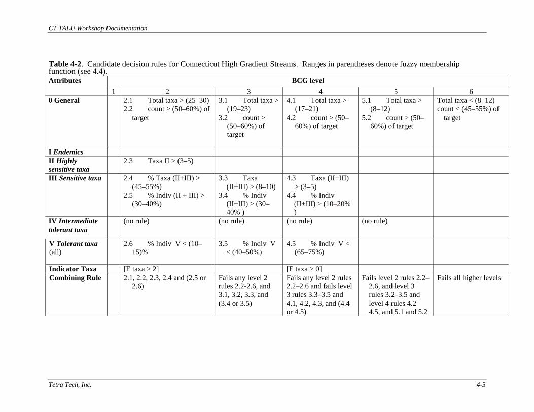
CT TALU Workshop Documentation
Tetra Tech, Inc. 4-5
Table 4-2. Candidate decision rules for Connecticut High Gradient Streams. Ranges in parentheses denote fuzzy membership function (see 4.4).
BCG level Attributes 1 2 3 4 5 6
0 General 2.1 Total taxa > (25–30) 2.2 count > (50–60%) of
target
3.1 Total taxa > (19–23)
3.2 count > (50–60%) of target
4.1 Total taxa > (17–21)
4.2 count > (50–60%) of target
5.1 Total taxa > (8–12)
5.2 count > (50–60%) of target
Total taxa < (8–12) count < (45–55%) of
target
I Endemics II Highly sensitive taxa
2.3 Taxa II > (3–5)
III Sensitive taxa 2.4 % Taxa (II+III) > (45–55%)
2.5 % Indiv (II + III) > (30–40%)
3.3 Taxa (II+III) > (8–10)
3.4 % Indiv (II+III) > (30–40% )
4.3 Taxa (II+III) > (3–5)
4.4 % Indiv (II+III) > (10–20% )
IV Intermediate tolerant taxa
(no rule) (no rule) (no rule) (no rule)
V Tolerant taxa (all)
2.6 % Indiv V < (10–15)%
3.5 % Indiv V < (40–50%)
4.5 % Indiv V < (65–75%)
Indicator Taxa [E taxa > 2] [E taxa > 0] Combining Rule 2.1, 2.2, 2.3, 2.4 and (2.5 or
2.6) Fails any level 2 rules 2.2-2.6, and 3.1, 3.2, 3.3, and (3.4 or 3.5)
Fails any level 2 rules 2.2–2.6 and fails level 3 rules 3.3–3.5 and 4.1, 4.2, 4.3, and (4.4 or 4.5)
Fails level 2 rules 2.2–2.6, and level 3 rules 3.2–3.5 and level 4 rules 4.2–4.5, and 5.1 and 5.2
Fails all higher levels

CT TALU Workshop Documentation
Tetra Tech, Inc. 4-6
4.3 BCG Level Descriptions Based on the characterization of sites identified as belonging to different BCG levels, we developed a set of linguistic rules for distinguishing levels. More complete description of the levels are in Appendix C. BCG level 2
• Total Taxon Richness: high • Total abundance: near target for subsample (200) • Highly sensitive taxa: At least some taxa are present • All sensitive taxa (highly sensitive + intermediate sensitive): comprise half or more
of all • All sensitive individuals: comprise 30% or more of all organisms • Tolerant individuals (tolerant + highly tolerant): a small fraction of all organisms
Based on the group decisions, the BCG level 2 rules 1–4 are “all or nothing”, that is, all must be met for a sample to be considered level 2. Logically, they are combined with AND operators. Rules 5 and 6 are less stringent: one of rules 5 and 6 must be met, but not both (joined with OR operator). The BCG level 2 rules discriminate level 2 from level 3 (and lower). BCG level 3
• Total Taxon Richness: moderate to high • Total abundance: near target for subsample
Highly sensitive taxa: may be absent (no rule)
• Richness of all sensitive taxa (highly sensitive + intermediate sensitive) is moderate • All sensitive individuals: comprise 30% or more of all organisms • Tolerant individuals (tolerant + highly tolerant): less than half of all individuals
As with BCG level 2, the relative abundance rules 4 and 5 are less stringent: one of rules 4 or 5 must be met, but not both (joined with OR operator). The BCG level 3 rules discriminate level 3 from level 4 (and lower). BCG level 4
• Total Taxon Richness: moderate to high • Total abundance: near target for subsample
Highly sensitive taxa: may be absent (no rule)
• All sensitive taxa (highly sensitive + intermediate sensitive) present but may be low
richness • All sensitive individuals: more than an insignificant fraction
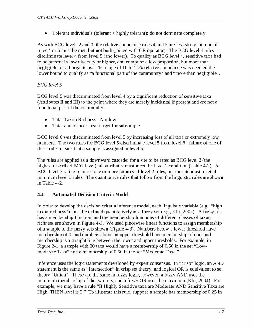
CT TALU Workshop Documentation
Tetra Tech, Inc. 4-7
• Tolerant individuals (tolerant + highly tolerant): do not dominate completely As with BCG levels 2 and 3, the relative abundance rules 4 and 5 are less stringent: one of rules 4 or 5 must be met, but not both (joined with OR operator). The BCG level 4 rules discriminate level 4 from level 5 (and lower). To qualify as BCG level 4, sensitive taxa had to be present in low diversity or higher, and comprise a low proportion, but more than negligible, of all organisms. The range of 10 to 15% relative abundance was deemed the lower bound to qualify as “a functional part of the community” and “more than negligible”. BCG level 5 BCG level 5 was discriminated from level 4 by a significant reduction of sensitive taxa (Attributes II and III) to the point where they are merely incidental if present and are not a functional part of the community.
• Total Taxon Richness: Not low • Total abundance: near target for subsample
BCG level 6 was discriminated from level 5 by increasing loss of all taxa or extremely low numbers. The two rules for BCG level 5 discriminate level 5 from level 6: failure of one of these rules means that a sample is assigned to level 6. The rules are applied as a downward cascade: for a site to be rated as BCG level 2 (the highest described BCG level), all attributes must meet the level 2 condition (Table 4-2). A BCG level 3 rating requires one or more failures of level 2 rules, but the site must meet all minimum level 3 rules. The quantitative rules that follow from the linguistic rules are shown in Table 4-2. 4.4 Automated Decision Criteria Model In order to develop the decision criteria inference model, each linguistic variable (e.g., “high taxon richness”) must be defined quantitatively as a fuzzy set (e.g., Klir, 2004). A fuzzy set has a membership function, and the membership functions of different classes of taxon richness are shown in Figure 4-3. We used piecewise linear functions to assign membership of a sample to the fuzzy sets shown (Figure 4-3). Numbers below a lower threshold have membership of 0, and numbers above an upper threshold have membership of one, and membership is a straight line between the lower and upper thresholds. For example, in Figure 2-1, a sample with 20 taxa would have a membership of 0.50 in the set “Low-moderate Taxa” and a membership of 0.50 in the set “Moderate Taxa.” Inference uses the logic statements developed by expert consensus. In “crisp” logic, an AND statement is the same as “Intersection” in crisp set theory, and logical OR is equivalent to set theory “Union”. These are the same in fuzzy logic, however, a fuzzy AND uses the minimum membership of the two sets, and a fuzzy OR uses the maximum (Klir, 2004). For example, we may have a rule “If Highly Sensitive taxa are Moderate AND Sensitive Taxa are High, THEN level is 2.” To illustrate this rule, suppose a sample has membership of 0.25 in
CT TALU Workshop Documentation
Tetra Tech, Inc. 4-8
the set: “Highly Sensitive taxa are Moderate” and membership of 0.75 in “Sensitive Taxa are High;” then its membership in level 2 is min(0.75, 0.25) = 0.25. Output of the inference model may include membership of a sample in a single level only, ties between levels, and varying memberships among two or more levels. The level with the highest membership value is taken as the nominal level.
Figure 4-3. Fuzzy set membership functions assigning linguistic values of Total Taxa to defined quantitative ranges. Heavy dashed line shows membership of fuzzy set defined by “Total taxa are moderate to high.”
4.4.1 Model Performance Model output is membership of a sample in each of the levels described in Table 3-2. In most cases, a single level is given a membership value of 1, and all the rest 0. Often, a single level will have a highest value and one or more other levels will be given a lower, non-zero membership value. We considered any two membership values within 0.1 as a tied decision between the levels. The fuzzy decision model was developed and calibrated with 48 high-gradient samples rated by the group. The final model treats the levels as a logical cascade from level 2 to level 6: failure of a rule for any level is considered a “success” for the next lower level. Overall, the decision model matched the panel decisions almost exactly: the nominal level of the fuzzy model exactly matched the workgroup nominal level assignments in 45 of 48 samples (94%). In all 3 cases where the model and the group did not agree, the respective minority and nominal choices were “flipped”. For example, for site CT 40-01, Clark Creek,
0
1
Total Taxa
Deg
ree
of m
embe
rshi
p
0 5 10 15 20 25 30 35
Low HighModerateLow-
moderate0.5

CT TALU Workshop Documentation
Tetra Tech, Inc. 4-9
the panel’s mean BCG level was 3.32, or a high-quality level 3, with a minority selection of level 2. The decision model was exactly tied between level 2 and level 3. Examination of the disagreements may also reveal inconsistencies by the human assessors; for example, the group may have assessed a sample as level 5 because of a single sensitive taxon among only 7 taxa total, while the rule had required more taxa to qualify for level 5. In other instances, the comparisons revealed the need for refining model calibration.
CT TALU Workshop Documentation
Tetra Tech, Inc. 5-1
5.0 MULTIMETRIC INDEX (MMI) A biological metric is a numerical expression of a biological community attribute that responds to human disturbance in a predictable fashion. Metrics were considered for inclusion in this multimetric index on the basis of discrimination efficiency, low inter-annual or seasonal variability, ecological meaningfulness, contribution of representative and unique information, and sufficient range of values. They were organized into seven categories: richness, composition, evenness, pollution tolerance, BCG attributes (Section 3.3), functional feeding group, and habit (mode of locomotion). 5.1 Metric Methods A suite of commonly applied, empirically proven, and theoretically responsive metrics was calculated for possible inclusion in a multimetric index. Tolerance metrics were based on both Hilsenhoff tolerance values and BCG taxa attribute groups (Davies and Jackson, 2006). Hilsenhoff tolerance values are on a 0 to 10 scale (most sensitive to most tolerant). The Hilsenhoff scale was derived primarily to address taxa tolerance to organic pollutants (Hilsenhoff, 1987). Attributes associated with taxa for BCG analysis range from sensitive-endemic to pollution tolerant. BCG attributes were assigned to taxa by consensus of a core group of agency biologists during a workshop conducted at DEP on September 6 and 7, 2006. All richness metrics (e.g., insect taxa and non-insect taxa) were calculated such that only unique taxa are counted. Those taxa that were identified at higher taxonomic levels because of damage or under-developed features were not counted as unique taxa if other individuals in the sample were identified to a lower taxonomic level within the same sample. Genus level taxonomy was expected to provide responsive metrics, so all metrics were calculated at the level. Metrics were calculated in a modified version of the Ecological Data Application System (EDAS), a Microsoft Access application. Once calculated, the metrics were imported into the statistical package Statistica for further analysis. Discrimination efficiency Discrimination efficiency (DE) is the capacity of the biological metric or index to detect stressed conditions. It is measured as the percentage of stressed sites that have values lower than the 25th percentile of reference values (Stribling et al., 2000). For metrics that increase with increasing stress, DE is the percentage of stressed sites that have values higher than the 75th percentile of reference values. DE can be visualized on box plots of reference and stressed metric or index values with the inter-quartile range plotted as the box (Figure 5-1). When there is no overlap of boxes representing reference and stressed sites, the DE is greater than 75%. A metric with a high DE thus has a greater ability to detect stress than a metric with a low DE. Metrics with DEs <25% do not discriminate and were not considered for inclusion in the index.

CT TALU Workshop Documentation
Tetra Tech, Inc. 5-2
Reference Stressed0
2
4
6
8
10
12
14
16
18
20
22
24
26
28EP
T Ta
xa
Median 25%-75% Non-Outlier Range Outliers
25th percentile of reference
DE = 100%: All stressed sites have metric values below the 25th percentile of reference
Figure 5-1. Illustration of metric discrimination efficiency (DE) between reference and stressed sites. Metric variability When comparing metrics, those with lower variability in the reference sites are preferable to those with higher variability. Variability was measured as the coefficient of variability (CV) in reference sites, calculated as the metric standard deviation over the mean, expressed as a percentage. Lower CVs indicate greater precision of metrics. Other metric considerations Ecologically meaningful metrics are those for which the assemblage response mechanisms are understandable and are represented by the calculated value. Ecological meaningfulness is a professional judgment based on theoretical or observed response mechanisms. Those metrics that respond according to expectations established in other studies are more defensible. Metrics contribute information representative of integrity if they are from diverse metric categories. As many metric categories as practical should be represented in an index so that signals of various stressors can be integrated into the index. While several metrics should be included to represent biological integrity, those that are included should not be redundant with each other. Redundancy was evaluated using Pearson product-moment correlation analysis. For metrics to discriminate on a gradient of stress, they must have a sufficient range of values. Metrics with limited ranges (e.g., richness of taxa poor groups or percentages of rare taxa) may

CT TALU Workshop Documentation
Tetra Tech, Inc. 5-3
have good discrimination efficiency. However, small metric value changes will result in large and perhaps meaningless metric scoring changes. Comprehensive metrics of sample composition were calculated in addition to the categorical metrics described above. RIVPACS provides a metric which compares the number of taxa expected to occur in reference sites with the number observed in test sites. After adjusting taxa counts for natural site classification variables, the observed to expected ratio (O/E) gives a measure of the degree to which the benthic sample reaches its potential richness. RIVPACS relies on cluster analysis of reference samples to identify naturally distinct community types; discriminant function analysis (DFA) to identify natural determinants of sites in the distinctive biological groupings; and models of expected and observed taxa; based on the predicted membership of a site in a group and of the probabilities of capturing each taxon in each site type. In the analysis, a null model was tested as a baseline for comparison of predictive precision in the final model. The null model does not account for natural variability and the final model does. 5.2 Metric Results Eighty (80) metrics were calculated in the seven metric categories. Within calibration samples, 51 metrics responded with at least 75 percent of stressed sites worse than the 25th or 75th percentile of reference (Appendix D). Metrics were excluded from consideration in possible index alternatives if they discriminated weakly between reference and stressed sites (DE < 75%), were redundant with more discriminating metrics, had limited ranges of values, or were not representative of the benthic community. RIVPACS Model The null RIVPACS model had an O/E mean and standard deviation of 1.00 and 0.21. The final model, accounting for catchment size, had an O/E mean and standard deviation of 1.07 and 0.19. The best RIVPACS models have means near 1.00 and standard deviations less than 0.20, optimally lower than 0.18. The model accounting for catchment size is slightly better than the null model because it has lower standard deviation (better precision). The discrimination efficiency of the final O/E index is 100%. Use of the O/E as an indicator has potential in Connecticut. However, it is not currently applicable because of computational complexities; calculation of O/E for new sites requires substantial software development and technology transfer to DEP. If O/E indices are pursued in the future, it would be worth exploring additional predictor variables, many of which can be obtained through remote (GIS) analysis. 5.3 Multimetric Index Composition A multimetric index is a combination of metric scores that indicates a degree of biological stress in the stream community (Barbour et al., 1999). Individual metrics are candidate for inclusion in the index if they
• discriminate well between reference and stressed sites; • are ecologically meaningful (mechanisms of responses can be explained); • represent diverse types of community information (multiple metric categories); and

CT TALU Workshop Documentation
Tetra Tech, Inc. 5-4
• are not redundant with other metrics in the index. Metrics are scored on a common scale prior to combination in an index. The scale ranges from 0 to 100 and the optimal score is determined by the distribution of data. For metrics that decrease with increasing stress, the 95th percentile of all high gradient data was considered optimal and scored as 100 points. All other metric values were scored as a percentage of the 95th percentile value (Figure 5-2) except those that exceeded 100, which were assigned a score of 100. The 95th percentile value was selected as optimal instead of the maximum so that outlying values would not skew the scoring scale.
Figure 5-2. Metric scoring schematic for metrics that decrease with increasing stress. For metrics that increased with increasing stress (not shown), the 5th percentile of the data was considered optimal and assigned a value of 100 points, with increasing values scaled down to 0. 5.4 Index Results Eleven index alternatives were calculated using an iterative process of adding and removing metrics, calculating the index, and evaluating index responsiveness and variability (Table 5-1). The first index alternatives included those metrics that had the highest DEs within each metric category. Subsequent index alternatives were formulated by adding, removing, or replacing one metric at a time from the initial index alternatives that performed well. The index alternatives did not exhaust the possible combinations of metrics. The few alternatives tested all discriminated reference and stressed sites completely—there was no overlap of index value distributions. Therefore the selection of metrics was more subjective than if there were extreme (or even meaningfully discernible) differences in index performance among index alternatives. The bias in metric selection was for those metrics that performed best
Met
ric V
alue
s
0
2
4
6
8
10
12
All samples Reference Degraded
Met
ric S
core
s
0
10
20
30
40
50
60
70
80
90
10095th%ile

CT TALU Workshop Documentation
Tetra Tech, Inc. 5-5
in each metric category, that have precedent in regional bioassessment indices, and that are not redundant either statistically or conceptually. An example of conceptually redundant metrics are the several measures based on BCG attributes (counts of attribute 3 taxa are conceptually redundant with % of attribute 3 taxa). Also, the number of metrics was limited to simplify index application. None of the community model metrics (O/E and PMA) were used in index alternatives for two reasons: to simplify application of the multimetric index and because metrics of this type are usually considered as stand-alone indicators. The final index alternative is one that met the criteria listed above and that performed best (high DE, low variability) among the alternatives tested. Each alternative index was evaluated based on discrimination efficiency (DE, calculated as for individual metrics), separation of reference and stressed index means as a multiple of the standard deviation reference scores (Z score), variability in reference sites, and verification results. Three indexes had Z scores above 5. The Z score is an expression of the statistical separation of the reference and stressed sites: the difference between reference mean and stressed mean, divided by the standard deviation of the reference sites. The selected index (#13 in Table 5-1) had a slightly higher Z-score and slightly lower coefficient of variation (CV) than the nearest contenders. The final index includes the following metrics:
• Ephemeroptera taxa (scoring adjusted for watershed area) • Plecoptera taxa • Trichoptera taxa • Percent sensitive EPT (scoring adjusted for watershed area) • Scraper taxa • BCG Taxa Biotic Index • Percent dominant genus
The selected index has a discrimination efficiency of 100%; all of the highly degraded sites have index values less than the 25th percentile of reference sites (Table 5-1). In fact, all of the degraded index values fall below the minimum of reference values (Figure 5-3). The verification data were comparable to calibration data.

CT TALU Workshop Documentation
Tetra Tech, Inc. 5-6
Table 5-1. Index alternatives 1–14, with metrics included in each metric and evaluation statistics. Metric DE 1 2 3 4 5 6 7 8 9 10 11 12 13* 14Total Taxa 100 2 3 4 5 6 7 8 9Non-Insect Taxa Percent 83.3 1EPT Taxa 100 1 8 11Ephemeroptera Taxa 100 2Ephemeroptera Taxa (adjusted for watershed area) 100 3 4 5 6 7 9 10 12 13 14
Plecoptera Taxa 100 2 3 4 5 6 7 9 10 12 13 14Trichoptera Taxa 83.3 2 3 4 5 6 7 9 10 12 13 14% EPT excluding Hydropsychidae and Baetidae 100 1 2% EPT excluding Hydropsychidae and Baetidae (adjusted for watershed area) 100 3 4 5 6 7 8 9 10 11 12 13 14
% Filterer 100 1% Predator 100 1 2 3 4 7Collector Taxa 100 9Scraper Taxa 100 2 3 4 5 6 7 8 10 11 12 13 14Biotic Index, Individual TALU Attributes 100 2 3 4 5 6 7 8 9 10 11Biotic Index, Taxa TALU Attributes 100 13 14Simpson's Index 100 4% dominant 1 91.7 2 3 6 9 10 11 12 13% Intolerant 100 1
DE calibration 100 100 100 100 100 100 100 100 100 100 100 100 100 100mean, all ref 74.3 73.0 75.5 75.4 76.9 78.0 74.2 80.1 76.7 77.5 81.0 77.8 77.9 76.6
stddev, all ref 16.1 12.3 12.1 12.5 12.1 11.5 12.6 12.8 11.4 11.4 12.1 10.7 10.5 11.2CV, ref 21.6 16.8 16.1 16.5 15.7 14.8 17.0 16.0 14.9 14.7 14.9 13.7 13.5 14.6
Cal Ref 25th %ile 56.2 62.2 71.3 71.1 71.0 72.7 69.2 71.7 71.7 72.7 73.0 73.7 72.2 70.0mean, all deg 18.8 19.3 20.5 17.9 18.2 21.8 17.2 19.5 22.9 20.5 22.8 22.7 20.9 16.6
Z-score ((Mean Ref - Mean Deg) / Stdev Ref) 3.5 4.4 4.5 4.6 4.8 4.9 4.5 4.7 4.7 5.0 4.8 5.2 5.4 5.3
CT TALU Workshop Documentation
Tetra Tech, Inc. 5-7
Ref Deg10
20
30
40
50
60
70
80
90
100R
ecom
men
ded
Inde
x
Figure 5-3. Index values in reference and degraded sites. Calibration data are shown in box plots, verification data are shown as individual points. The BCG taxa biotic index is the average attribute value for all taxa in the sample (attribute 5a was given a value of 6 so that it could be averaged). Performance statistics and scoring formulas of the index metrics (Table 5-2) will allow application and interpretation of the index. Investigators should calculate scores from sample taxa lists (using genus level taxonomy) and average the scores to arrive at the appropriate index value. Total taxa is in several of the index alternatives, but it was dropped from the final because it is borderline redundant (correlation coefficient near 0.80) with Trichoptera taxa, scraper taxa, and the BCG taxa biotic index. The strongest correlations among index metrics were between BCG taxa biotic index and both Ephemeroptera taxa and Plecoptera taxa, with a correlation coefficient of -0.76 (Table 5-3). This level of redundancy is acceptable.
CT TALU Workshop Documentation
Tetra Tech, Inc. 5-8
Table 5-2. Performance statistics and scoring formulas for index metrics. Metric CV 1 DE 2 Response 3 Scoring Formula 4 Ephemeroptera taxa 5 18.7 100 Dec = 100* (X + 1.4) / 8.5 Plecoptera taxa 45.5 100 Dec = 100* X / 6 Trichoptera taxa 33.8 83.3 Dec = 100* X / 13 % sensitive EPT 5 31.3 100 Dec = 100* (X + 9.2) / 75.2 Scraper taxa 30.1 100 Dec = 100* X / 11 BCG Taxa Biotic Index 6.3 100 Inc = 100*(4.6-X) / 1.5 % dominant genus 41.0 91.7 Inc = 100*(85-X) / 73
1 CV = Coefficient of Variability = 100*StdDevRef / MeanRef. 2 DE = Discrimination Efficiency = percentage of degraded samples with metric values outside of the
reference quartile range in the direction of response (calibration data only). 3 Direction of metric response with increasing stress, decreasing (Dec) or increasing (Inc). 4 The scoring range is between 0 and 100. If formula results in a value outside of the range, reset the
score to the nearest extreme of the range. 5 See Table 2-3 for metric adjustment prior to scoring Table 5-3. Correlations (Pearson r) among index metrics.
# Metric 1 2 3 4 5 6 7 1 Ephemeroptera taxa (adj.) • 2 Plecoptera taxa 0.58 • 3 Trichoptera taxa 0.57 0.50 • 4 % sensitive EPT (adj.) 0.69 0.54 0.52 • 5 Scraper taxa 0.67 0.50 0.75 0.52 • 6 BCG Taxa Biotic Index -0.76 -0.76 -0.68 -0.74 -0.69 • 7 % dominant genus -0.61 -0.54 -0.62 -0.59 -0.60 0.66 •

CT TALU Workshop Documentation
Tetra Tech, Inc. 6-1
6.0 DISCUSSION AND CONCLUSIONS 6.1 BCG and MMI Concordance The MMI uses metrics that are similar in objective to the BCG attributes but calculated somewhat differently (e.g., EPT taxa metrics in the MMI include taxa considered to be Attributes II, III, IV; and Attribute II includes taxa from the EPT orders, as well as a few dipteran and beetle taxa). The total MMI score is based on the average of all metrics, while BCG decisions are based on decision-specific critical attribute groups; e.g., Attributes II and III for the higher levels and Attribute V for lower levels. Concordance of the two assessment endpoints is strong (Figures 6-1−6-2). Figure 6-1 shows the BCG calibration data as rated by the panel, and Figure 6-2 shows the predicted results of the BCG model. In spite of these differences, MMI scores could be used to separate levels (Figures 6-1, 6-2). Potential MMI scoring thresholds could be as follows:
BCG level MMI Scoring Range levels 1, 2 MMI > 75 level 3 75 ≥ MMI > 60 level 4 60 ≥ MMI > 43 level 5 43 ≥ MMI > 20 level 6 20 ≥ MMI
6.2 Variability Data from a set of 20 sites that had been sampled in multiple years were analyzed for variability. The sites were selected on the basis of greater land use, land cover, and disturbance stability over the sampling period, that is, these sites had no major construction, development, restoration, or discharge upgrades in the period between samples. Some of the sites were protected, and some were in heavily disturbed areas. Stations were sampled 2–8 times over time periods of 1 to 10 years; consecutive samples were separated by 1 to 8 years The data collected by Connecticut, and the indexes derived from them, show remarkable stability when samples from the same sites are compared among years (Figure 6-3, Table 6-1). The maximum difference within sites was 21 points of the MMI, and 1 level of the BCG. With respect to BCG levels, 16 of the 20 sites were stable within a single level with at most a single observation rated in an adjacent level. Two sites appeared to be intermediate between adjacent levels, with 2 or more observations rated in each level (Eightmile River and Roaring Brook).
CT TALU Workshop Documentation
Tetra Tech, Inc. 6-2
102030405060708090100
CT MMI
2.0
2.5
3.0
3.5
4.0
4.5
5.0
5.5
6.0
6.5
Mea
n B
CG
Tie
r Reference Degraded Other
Sages Ravine
West Branch Naugatuck
Tier 6
Tier 2
Tier 5
Tier 4
Tier 3
Figure 6-1. Comparison of index values and mean BCG levels (from group development), with outliers labeled. Horizontal lines indicate nominal BCG levels.
Median 25%-75% Non-Outlier Range OutliersExtremes2 3 4 5 6
Model Tier (nominal)
0
10
20
30
40
50
60
70
80
90
100
Mul
timet
ric In
dex
32 2744189
Figure 6-2. Connecticut Multimetric index by BCG levels, estimated from decision analysis model. Number of samples given below boxes.
CT TALU Workshop Documentation
Tetra Tech, Inc. 6-3
Tier 2 Tier 3 Tier 4 Tier 5 Tier 6
Eig
htm
ile R
Gre
en F
all R
Har
bor B
rLi
ttle
RM
atta
bess
et R
Nat
chau
g R
Nau
gatu
ck R
14
Nau
gatu
ck R
26A
Nau
gatu
ck R
15
Peq
uabu
ck R
Qua
ker B
rR
oarin
g B
rSa
lmon
RS
andy
Br
Sau
gatu
ck R
She
paug
RSh
unoc
k R
Titic
us R
W B
Nau
gatu
ckW
hitfo
rd B
r
Waterbody
0
10
20
30
40
50
60
70
80
90
100
110C
T M
MI
Model Tier
Figure 6-3. Nominal BCG assessments and IBI scores for 20 sites with repeated samples. Table 6-1. Variability of indexes and metrics from multiyear observations Quantity Range s.d. Approx. 95% C.I. BCG Nominal level 2 - 6 0.396 0.78 BCG Average level 2 - 6 0.382 0.75 Multimetric Index 0 - 100 5.41 10.6
% Dominant taxon 0 - 100 11 21.56 Plecoptera taxa 0 - 8 1.08 2.12 Scraper taxa 0 - 14 1.24 2.43 Ephemeroptera taxa 0 - 12 0.994 1.94 % Sensitive EPT 0 - 90 10.2 19.99 Trichoptera taxa 2 - 18 1.426 2.79 BCG Attribute index 2 - 6 0.141 0.276
The repeated observations (Figure 6-3, Table 6-1) demonstrate that the Connecticut methodology has low inherent variability in measurements taken among years. Each of the metrics has a standard deviation that is approximately 7–10% of the expected range of the metric. Such stability among years, at sites with no known changes in anthropogenic sources and stressors,
CT TALU Workshop Documentation
Tetra Tech, Inc. 6-4
indicates that the methods and analysis are stable over time. Natural variability is confined to a single BCG level, or about 20 points on the MMI scale. Demonstration that a site has consistently shifted a single BCG level, or 20 MMI points, is positive indication of a change in stress level at the site (increase or decrease), beyond that expected due to natural variability. We also examined whether there was an association between the biological scores and potential drought stress in the streams. We used the Palmer hydrological drought Index (PHDI), obtained from the National Climatic Data Center (www.ncdc.noaa.gov). There were no severe drought years in the data set, and there was no association between biological scores (MMI or BCG level) and the PHDI, within the range of the PHDI observed in these streams (-1.5 to + 3.5; or mild drought to moderately wet). 6.3 The BCG as an Assessment Tool The BCG, as developed conceptually in Davies and Jackson (2006), addresses several limitations of existing biotic indexes. Advantages of the BCG include (Gerritsen et al., submitted):
• The BCG is based on ecological considerations with wide expert agreement, rather than on empirical analysis of a particular data set. It is calibrated using a data set, but the result is intended to be more general than a regression analysis of biological response to stressors.
• The BCG uses universal attributes (Attributes I to VI) that are intended to apply in all
regions. Specifics of the attributes (taxon membership, attribute levels indicating good, fair, poor, etc.) do vary across regions and stream types, but the attributes themselves and their importance are consistent.
• The BCG requires descriptions of the classes or levels, from pristine to degraded . While
requiring extra work, this ensures that future information and discoveries can be related back to the baseline level descriptions. Levels are not perfect or static—they will be altered by increase in knowledge.
The BCG may be more robust than current indexes because it allows, in some cases, for nonlinear responses. The BCG is not conceptually tied to “best available” sites as a reference condition: although best available sites are used as a practical ground truth, it is recognized at the outset that these sites are typically less than pristine, and may be a lower level (e.g., 2, 3, 4). Implementation will be made more consistent with automated methods to assign sites to levels. At the simplest level, an IBI score range or metric, or a RIVPACs-based observed/expected score range (e.g., Barbour et al., 1999) can be divided into classes corresponding to levels developed here. The IBI and RIVPACs models characterize a gradient, but they do not necessarily reflect the professional consensus that goes into the level descriptions. An alternative is to develop a scoring model that replicates the professional consensus in the level descriptions, either by statistical inference (e.g., Davies et al. 1993) or by direct replication of the rules.

CT TALU Workshop Documentation
Tetra Tech, Inc. 6-5
6.4 The BCG and Aquatic Life Use The terms “Use”, “Designated Uses”, and “Aquatic Life Use” have specific meanings for water quality management in the context of the Clean Water Act. A state defines the uses for its waters, and develops physical, chemical and biological criteria to protect those uses. TALUs are aquatic life uses that are matched more closely to the Designated Uses, rather than a single one-size-fits-all aquatic life use (EPA, 2005). The BCG is a scientific model of biological condition of waters, set on a universal scale from natural and undisturbed (BCG level 1) to completely biologically and ecologically disrupted (BCG level 6). The BCG, as a universal yardstick, is intended to be used in setting biological criteria to match specific TALUs. It is important to note that levels of the BCG are NOT equivalent to TALUs. The BCG is a scientific measurement yardstick only; it does not express policy decisions and breakpoints for designated uses. Designated Uses are intended to be set at the highest attainable use for a water body, taking into account natural limitations or irreversible physical (infrastructure) alterations to the habitat or watershed (e.g., existing urban infrastructure, flood control, harbor facilities, irrigation, etc.). Infrastructure is not always irreversible: roads can be rerouted, many older dams and obstructions are being removed from streams, habitat can be restored, etc. Designated uses thus also include potential quality or condition that may not currently be attained, but could be attained with appropriate controls or restoration. Thus, Aquatic Life Uses must be set according to the biological potential of waterbodies, not according to their current condition. The BCG, as a scientific measurement tool, does not explicitly include assessment of potential condition. The restoration potential of an impaired water body can only be predicted scientifically if the cause of impairment is known, that is, if we know what to do to restore the waterbody, and hence, we know which stressors will be reduced. Setting of designated uses, which implies a restoration goal, does not require causal analysis, because the designated uses are societal decisions on the desired state of a waterbody, and are determined by existing highest uses and watershed/habitat alterations deemed irreversible by the state (and existing as of 1976). The levels of the BCG are biologically recognizable stages in condition of stream waterbodies. As such, they can form a biological basis for criteria and regulation of a state’s waterbodies. Current thresholds of biocriteria in many states (usually an IBI score, or something similar) are relatively low (e.g., level 4-level 5), and fail to protect outstanding condition waters (levels 1 and 2), or even good condition waters (level 3). Thus, biocriteria set at a lower BCG level will allow incremental degradation of waterbodies to the regulatory level. The BCG provides a powerful approach for an operational monitoring and assessment program, for communicating resource condition to the public and for management decisions to protect or remediate water resources. The BCG and the calibrated decision system allow practical and operational implementation of multiple aquatic life uses in a state’s water quality criteria and standards. Adoption of the BCG as an assessment tool in the context of multiple Aquatic Life Uses (Tiered Uses) yields the technical tools for protecting the state’s highest quality waters, as well as developing realistic restoration goals for urban and agricultural waters.
CT TALU Workshop Documentation
Tetra Tech, Inc. 6-6
Connecticut could use the BCG, or an IBI index calibrated to the BCG, to identify biological expectations for tiered aquatic life uses. Several of the stream sites in least-stressed catchments in this report were rated a BCG level 2 by the panel of biologists. The least-stressed catchments may also correspond to Outstanding or Exceptional waters (this would need to be confirmed). Accordingly, the biological criterion for these waters could be BCG level 2 or better. 6.5 Technical Recommendations The Connecticut BCG is promising as a basis for decision criteria for Tiered Aquatic Life Use development. Results reported here should be confirmed and reviewed to address discrepancies between the BCG and MMI, and to examine outlier sites. The BCG description and rules can be tested and recalibrated, and Connecticut’s monitoring program can be strengthened to support use of the BCG: Develop BCG for low gradient streams. Connecticut’s sampling and assessment has been developed and calibrated for high-gradient streams, because these are by far the dominant stream resource. Nevertheless, low gradient streams are common in coastal areas, and occur throughout the state. They are dominated by sandy stream bottom, and principal invertebrate habitat consists of snags, root wads, undercut banks, and emergent vegetation. Standardized high-gradient methods (mid-stream sampling) applied to low-gradient streams often results in low richness and dominance of organisms adapted to fine sediment. Development of a BCG for the low gradient streams would require a data set sampled with low-gradient methods (Barbour et al., 1999), with similar numbers of samples in reference and highly-stressed sites. Develop BCG for a second assemblage. Two assemblages do not respond to stressors in exactly the same way and would not always agree in assessments. Fish may not be sampled (nor need to be) at all locations where benthic macroinvertebrates are sampled – assessments can be made from benthic macroinvertebrates alone, but the fish (or other assemblages) may indicate problems or issues that the invertebrates do not. Assessments based on fish are less reliable in small headwater streams (Yoder and Rankin, 1995). In Ohio, full attainment requires that both assemblages and all indexes meet the biocriteria, nonattainment of one but not both assemblages results in a rating of “partial attainment” (Yoder and Rankin, 1995). Search for level 1 sites. No sites sampled met the NEWS criteria for Minimally Disturbed (Snook et al., 2007; Stoddard et al., 2006). Biological and ecological attributes for level 1 should also include a second assemblage of the spatial attributes, (IX and X), and the endemic-rare species attributes (Attribute I). Candidate minimally disturbed sites could be found in neighboring states (Massachusetts, New York, northern Pennsylvania).

CT TALU Workshop Documentation
Tetra Tech, Inc. 7-1
7.0 LITERATURE CITED Barbour, M.T., J. Gerritsen, B.D. Snyder, and J.B. Stribling. 1999. Rapid Bioassessment Protocols for Use in Streams and Wadeable Rivers: Periphyton, Benthic Macroinvertebrates and Fish. Second Edition. EPA/841-B-99-002. U.S. EPA, Office of Water, Washington, D.C. Bell, M. 1985. The Face of Connecticut. Bulletin 110, State Geological and Natural History Survey of Connecticut, Hartford, CT. Buchwalter, D.B. and S.N. Luoma. 2005. Differences in dissolved cadmium and zinc uptake among stream insects: mechanistic explanations. Environ. Sci. Technol. 39:498-504. Cairns, J. Jr., P.V. McCormick and B.R. Niederlehner. 1993. A proposed framework for developing indicators of ecosystem health. Hydrobiologia 263:1-44. Cairns, J. Jr., and J.R. Pratt. 1993. A history of biological monitoring using benthic macroinvertebrates. Pages 10-27 in D.M. Rosenberg and V.H. Resh (editors). Freshwater Biomonitoring and Benthic Macroinvertebrates. Chapman and Hall, Inc., New York. Castella, E. and M.C.D. Speight. 1996. Knowledge representation using fuzzy coded variables: an example based on the use of Syrphidae (Insecta, Diptera) in the assessment of riverine wetlands. Ecol. Model. 85:13-25. Clarke, R.T., M.T. Furse, J.M. Wright, and D. Moss. 1996. Derivation of a biological quality index for river sites: comparison of the observed with the expected fauna. J. Appl. Stat. 23:311-322. Connecticut DEP. 2005. Connecticut Comprehensive Ambient Water Quality Monitoring Strategy. Connecticut Department of Environmental Protection, Bureau of Water Management, Hartford, CT. Connecticut DEP. 2004. Ambient Water Quality Monitoring: Rotating Basin Approach Data Summary (1996-2001). Draft report. Connecticut Department of Environmental Protection, Bureau of Water Management, Hartford, CT. Davies, S.P., and S.K. Jackson, 2006. The Biological Condition Gradient: A descriptive model for interpreting change in aquatic ecosystems. Ecol.ogical Applic. 16:1251-1266. Davies, S. P., L. Tsomides, D. L. Courtemanch, and F. Drummond. 1995. Maine biological monitoring and biocriteria development program. Maine Department of Environmental Protection, Bureau of Water Quality Control. DEP-LW108. Demicco, R.V. 2004. Fuzzy Logic and Earth Science: An Overview. In Fuzzy Logic in Geology, R.V. Demicco and G.J. Klir (eds.), pp. 11-61. Elsevier Academic Press, San Diego, CA.

CT TALU Workshop Documentation
Tetra Tech, Inc. 7-2
Demicco, R.V., and G.J. Klir. 2004. Introduction. In Fuzzy Logic in Geology, R.V. Demicco and G.J. Klir (eds.), pp. 1-10. Elsevier Academic Press, San Diego, CA. Gerritsen, J., and M. J. Paul. 2006. Statistical guidance for developing biological indicators for rivers and streams: A Guide for constructing multimetric and multivariate predictive bioassessment models. USEPA, Office of Research and Development and Office of Science and Technology, Washington, DC. (in press). Gerritsen, J., J.G. Kennen, J. Kurtenbach, D. Bryson, V. Poretti, J. Bower-Altman, E.W. Leppo, and K. Berry. In review. Decision criteria for assessing aquatic biological condition: A practical application. Submitted to Environmental Management. Hilsenhoff, W.L. 1987. An improved biotic index of organic stream pollution. Gt. Lakes Entomol. 20:31-39. Ibelings, B.W., M Vonk, H.F.J. Los, D.T. Van Der Molen, and W.M. Mooij. 2003. Fuzzy modeling of Cyanobacterial surface waterblooms: validation with NOAA-AVHRR satellite images. Ecological Applications 13:1456-1472.Hilsenhoff 1987 Karr, J.R. and E. W. Chu. 1999. Restoring Life In Running Waters: Better Biological Monitoring. Island Press, Washington, DC. Karr, J.R., K.D. Fausch, P.L. Angermeier, P.R. Yant, and I.J. Schlosser. 1986. Assessing biological integrity in running waters: A method and its rationale. Special publication 5. Illinois Natural History Survey. Klir, G.J. 2004. Fuzzy Logic: A Specialized Tutorial. In Fuzzy Logic in Geology, R.V. Demicco and G.J. Klir (eds.), pp. 11-61. Elsevier Academic Press, San Diego, CA. Maizel, M., R.D. White, R. Root, S. Gage, S. Stitt, L. Osborne, and G. Muehlbach. 1998. Historical Interrelationships Between Population Settlement and Farmland in the Conterminous United States, 1790 to 1992. Ch. 2 in Sisk, T.D., editor. 1998. Perspectives on the land-use history of North America: a context for understanding our changing environment. U.S. Geological Survey, Biological Resources Division, Biological Science Report USGS/BRD/BSR 1998-0003 (Revised September 1999). 104 pp. http://biology.usgs.gov/luhna/cover.html McCune, B., and I.B. Grace. 2002. Analysis of Ecological Communities. MJM Software Design, Dunedin Beach, OR. Plafkin, J.L., M.T. Barbour, K.D. Porter, S.K. Gross, and R.M. Hughes. 1989. Rapid bioassessment protocols for use in streams and rivers: Benthic macroinvertebrates and fish. EPA/440/4-89/001. U.S. EPA Office of Water, Washington, DC.

CT TALU Workshop Documentation
Tetra Tech, Inc. 7-3
Simpson, J.C and R.H. Norris. 2000. Biological assessment of river quality: development of AusRivAS models and outputs. In Assessing the Biological Quality of Fresh Waters: RIVPACS and Other Techniques. J.F. Wright, D.W. Sutcliffe and M.T. Furse (eds.), pp. 125-142. Freshwater Biological Association, Ambleside, UK. Snook, H., S.P. Davies, J. Gerritsen, B.K. Jessup, R. Langdon, D. Neils, and E. Pizutto. 2007. The New England Wadeable Stream Survey (NEWS): Development of Common Assessments in the Framework of the Biological Condition Gradient. U.S. EPA and New England Interstate Water Pollution Control Commission. Stoddard, J.L., D.P. Larsen, C.P. Hawkins, R.K. Johnson, and R.H. Norris. 2006. Setting expectations for the ecological condition streams: The concept of reference condition. Ecol. Applic. 16:1267-1276. U.S. Environmental Protection Agency (USEPA). 2005. Use of Biological Information to Better Define Designated Aquatic Life Uses in State and Tribal Water Quality Standards. Tiered Aquatic Life Uses. Public Science Review Draft. EPA-822-R-05-001. Wright, J.F. 2000. An introduction to RIVPACS. In Assessing the Biological Quality of Fresh Waters: RIVPACS and Other Techniques. J.F. Wright, D.W. Sutcliffe and M.T. Furse (eds.), pp. 1-24. Freshwater Biological Association, Ambleside, UK. Yoder, C.O. and E.T. Rankin. 1995. Biological criteria program development and implementation in Ohio. In Biological assessment and criteria: tools for water resource planning and decision making, Davis, W.S. and Simon, T.P. (eds.), pp. 109-144. Lewis Publishers, Boca Raton, FL.

APPENDIX A
CONNECTICUT INVERTEBRATE TAXA LIST AND ATTRIBUTE ASSIGNMENTS

Class or Order Family GenusBCG
AttributeHBI
ToleranceNo. of
IndividualsNo. of
SamplesHirudinea Erpobdellidae 5.5 8 1 1Hirudinea Erpobdellidae Erpobdella 5.5 8 89 18Hirudinea Erpobdellidae Nephelopsis 5.5 8 1 1Hirudinea Glossiphoniidae Glossiphonia 5.5 6 1 1Hirudinea Glossiphoniidae Helobdella 5.5 10 1 1Oligochaeta x 9 4 3Oligochaeta Enchytraeidae 3 8 24 14Oligochaeta Lumbricidae x 10 2 1Oligochaeta Lumbricidae Lumbricina 4 8 51 5Oligochaeta Naididae 4 8 23 4Oligochaeta Naididae Dero x 10 1 1Oligochaeta Naididae Nais 4 8 19 12Oligochaeta Naididae Pristinella x 7 1Oligochaeta Tubificidae 5 10 362 84Oligochaeta Tubificidae Aulodrilus 5 8 8 1Oligochaeta Tubificidae Limnodrilus 5 10 20 1Oligochaeta Lumbriculidae 4 8 326 55Acari 4 4 28 20Acari Lebertiidae Lebertia 4 4 6 1Acari Limnocharidae Rhyncholimnochares 4 4 3 3Acari Sperchonidae Sperchon 4 4 6 5Acari Sperchonidae Sperchonopsis 4 4 9 6Acari Torrenticolidae Torrenticola 4 4 6 6Collembola x 5 2 1Coleoptera Dryopidae Helichus 4 5 6 5Coleoptera Dytiscidae Dytiscidae 4 5 1 1Coleoptera Elmidae Ancyronyx 4 6 12 12Coleoptera Elmidae Dubiraphia 4 6 58 24Coleoptera Elmidae Elmidae 4 4 67 23Coleoptera Elmidae Macronychus 4 4 40 29Coleoptera Elmidae Microcylloepus 4 3 49 23Coleoptera Elmidae Optioservus 4 3 1913 210Coleoptera Elmidae Oulimnius 3 4 425 110Coleoptera Elmidae Promoresia 3 3 549 99Coleoptera Elmidae Stenelmis 4 5 1239 174Coleoptera Hydrochidae Hydrochus 5 1 1Coleoptera Hydrophilidae Berosus 5 22 11Coleoptera Psephenidae Ectopria 3 5 99 50Coleoptera Psephenidae Psephenus 3 4 1748 177Coleoptera Ptilodactylidae Anchytarsus 3 2 76 23Diptera x 8 4Diptera Athericidae Atherix 3 2 131 50Diptera Ceratopogonidae Bezzia 3 6 17 16Diptera Ceratopogonidae Ceratopogoninae 3 6 1 1Diptera Chironomidae x 7 342 69Diptera Chironomidae Brillia 4 5 39 31Diptera Chironomidae Cardiocladius 5.5 5 54 26Diptera Chironomidae Chaetocladius x 1 1Diptera Chironomidae Chironomini 4 7 6 4Diptera Chironomidae Chironomus 5 10 8 6
CT Data
A-1
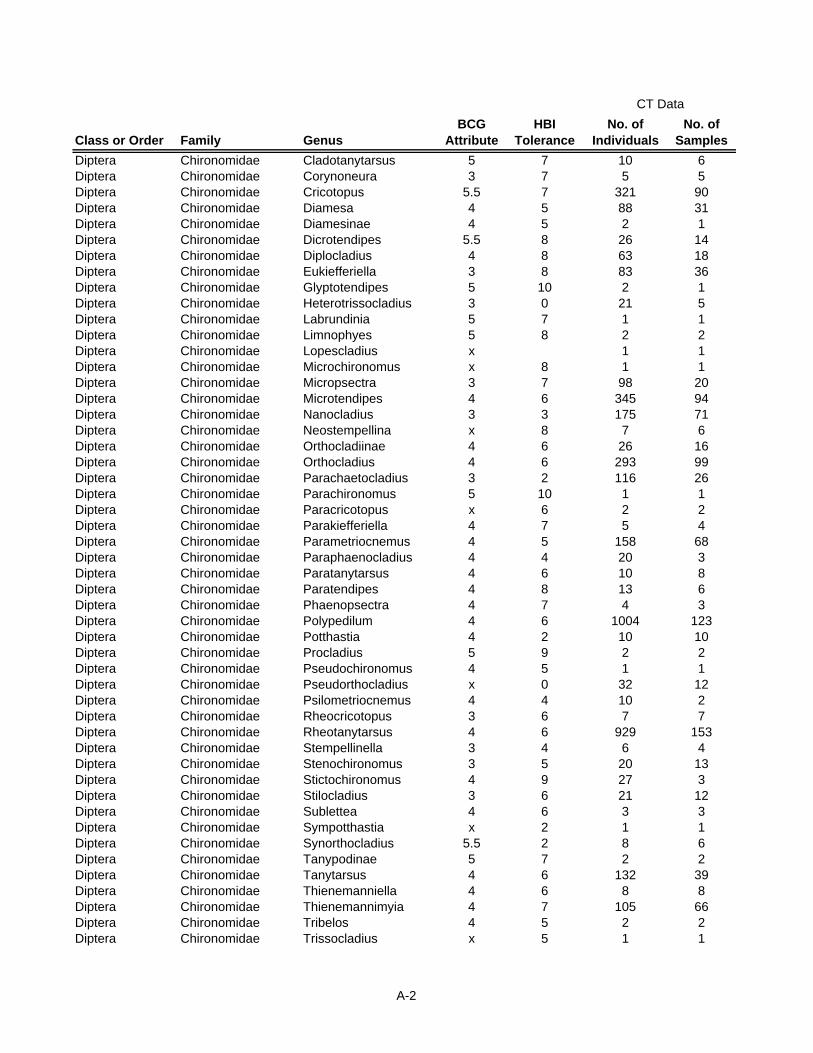
Class or Order Family GenusBCG
AttributeHBI
ToleranceNo. of
IndividualsNo. of
Samples
CT Data
Diptera Chironomidae Cladotanytarsus 5 7 10 6Diptera Chironomidae Corynoneura 3 7 5 5Diptera Chironomidae Cricotopus 5.5 7 321 90Diptera Chironomidae Diamesa 4 5 88 31Diptera Chironomidae Diamesinae 4 5 2 1Diptera Chironomidae Dicrotendipes 5.5 8 26 14Diptera Chironomidae Diplocladius 4 8 63 18Diptera Chironomidae Eukiefferiella 3 8 83 36Diptera Chironomidae Glyptotendipes 5 10 2 1Diptera Chironomidae Heterotrissocladius 3 0 21 5Diptera Chironomidae Labrundinia 5 7 1 1Diptera Chironomidae Limnophyes 5 8 2 2Diptera Chironomidae Lopescladius x 1 1Diptera Chironomidae Microchironomus x 8 1 1Diptera Chironomidae Micropsectra 3 7 98 20Diptera Chironomidae Microtendipes 4 6 345 94Diptera Chironomidae Nanocladius 3 3 175 71Diptera Chironomidae Neostempellina x 8 7 6Diptera Chironomidae Orthocladiinae 4 6 26 16Diptera Chironomidae Orthocladius 4 6 293 99Diptera Chironomidae Parachaetocladius 3 2 116 26Diptera Chironomidae Parachironomus 5 10 1 1Diptera Chironomidae Paracricotopus x 6 2 2Diptera Chironomidae Parakiefferiella 4 7 5 4Diptera Chironomidae Parametriocnemus 4 5 158 68Diptera Chironomidae Paraphaenocladius 4 4 20 3Diptera Chironomidae Paratanytarsus 4 6 10 8Diptera Chironomidae Paratendipes 4 8 13 6Diptera Chironomidae Phaenopsectra 4 7 4 3Diptera Chironomidae Polypedilum 4 6 1004 123Diptera Chironomidae Potthastia 4 2 10 10Diptera Chironomidae Procladius 5 9 2 2Diptera Chironomidae Pseudochironomus 4 5 1 1Diptera Chironomidae Pseudorthocladius x 0 32 12Diptera Chironomidae Psilometriocnemus 4 4 10 2Diptera Chironomidae Rheocricotopus 3 6 7 7Diptera Chironomidae Rheotanytarsus 4 6 929 153Diptera Chironomidae Stempellinella 3 4 6 4Diptera Chironomidae Stenochironomus 3 5 20 13Diptera Chironomidae Stictochironomus 4 9 27 3Diptera Chironomidae Stilocladius 3 6 21 12Diptera Chironomidae Sublettea 4 6 3 3Diptera Chironomidae Sympotthastia x 2 1 1Diptera Chironomidae Synorthocladius 5.5 2 8 6Diptera Chironomidae Tanypodinae 5 7 2 2Diptera Chironomidae Tanytarsus 4 6 132 39Diptera Chironomidae Thienemanniella 4 6 8 8Diptera Chironomidae Thienemannimyia 4 7 105 66Diptera Chironomidae Tribelos 4 5 2 2Diptera Chironomidae Trissocladius x 5 1 1
A-2
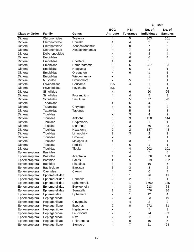
Class or Order Family GenusBCG
AttributeHBI
ToleranceNo. of
IndividualsNo. of
Samples
CT Data
Diptera Chironomidae Tvetenia 4 5 303 101Diptera Chironomidae Unniella 4 4 2 2Diptera Chironomidae Xenochironomus 2 0 7 6Diptera Chironomidae Xestochironomus x 7 4 3Diptera Dolichopodidae x 4 4 4Diptera Empididae 4 6 6 4Diptera Empididae Chelifera 4 6 5 5Diptera Empididae Hemerodromia 5 6 237 93Diptera Empididae Neoplasta x 6 1 1Diptera Empididae Oreogeton x 6 1 1Diptera Empididae Wiedemannia x 1 1Diptera Muscidae Limnophora x 5 1 1Diptera Psychodidae Pericoma 5.5 4 1 1Diptera Psychodidae Psychoda 5.5 1 1Diptera Simuliidae x 6 50 25Diptera Simuliidae Prosimulium 4 4 5 3Diptera Simuliidae Simulium 5 5 331 90Diptera Tabanidae 4 6 4 3Diptera Tabanidae Chrysops 4 6 5 2Diptera Tabanidae Tabanus 4 5 3 3Diptera Tipulidae x 3 4 2Diptera Tipulidae Antocha 5 3 458 144Diptera Tipulidae Cryptolabis 2 3 1 1Diptera Tipulidae Dicranota 3 3 70 33Diptera Tipulidae Hexatoma 2 2 137 48Diptera Tipulidae Limnophila 2 3 2 2Diptera Tipulidae Limonia x 4 1Diptera Tipulidae Molophilus 4 3 2 1Diptera Tipulidae Pedicia x 6 1 1Diptera Tipulidae Tipula 4 4 202 101Ephemeroptera Baetidae 4 4 7 5Ephemeroptera Baetidae Acentrella 4 4 376 106Ephemeroptera Baetidae Baetis 4 5 619 102Ephemeroptera Baetidae Plauditus 3 4 16 5Ephemeroptera Baetiscidae Baetisca 3 3 3 2Ephemeroptera Caenidae Caenis 4 7 6 4Ephemeroptera Ephemerellidae 3 1 26 11Ephemeroptera Ephemerellidae Dannella 2 2 1 1Ephemeroptera Ephemerellidae Ephemerella 3 1 1600 145Ephemeroptera Ephemerellidae Eurylophella 4 3 213 74Ephemeroptera Ephemerellidae Serratella 3 2 476 86Ephemeroptera Ephemeridae Ephemera 2 1 12 4Ephemeroptera Heptageniidae x 4 63 19Ephemeroptera Heptageniidae Cinygmula x 4 2 2Ephemeroptera Heptageniidae Epeorus 2 0 272 51Ephemeroptera Heptageniidae Heptagenia x 5 3Ephemeroptera Heptageniidae Leucrocuta 2 1 74 33Ephemeroptera Heptageniidae Nixe x 2 1 1Ephemeroptera Heptageniidae Rhithrogena 2 0 10 5Ephemeroptera Heptageniidae Stenacron 4 7 51 24
A-3

Class or Order Family GenusBCG
AttributeHBI
ToleranceNo. of
IndividualsNo. of
Samples
CT Data
Ephemeroptera Heptageniidae Stenonema 4 3 3294 235Ephemeroptera Isonychiidae Isonychia 3 2 3108 173Ephemeroptera Leptophlebiidae 2 2 331 57Ephemeroptera Leptophlebiidae Habrophlebiodes 4 6 1 1Ephemeroptera Leptophlebiidae Leptophlebia 2 4 8 4Ephemeroptera Leptophlebiidae Paraleptophlebia 2 1 191 23Ephemeroptera Potamanthidae Anthopotamus 2 4 9 7Hemiptera Sialidae Sialis 3 4 38 27Hemiptera Veliidae Microvelia x 2 1Hemiptera Veliidae Rhagovelia x 2 2Lepidoptera x 5 2 2Lepidoptera Pyralidae x 5 1 1Lepidoptera Pyralidae Paraponyx x 5 1 1Lepidoptera Pyralidae Petrophila x 5 16 10Megaloptera Corydalidae Corydalus 3 6 197 87Megaloptera Corydalidae Nigronia 3 4 792 186Odonata Aeshnidae Boyeria 4 2 45 31Odonata Calopterygidae Calopteryx 4 5 26 18Odonata Coenagrionidae 4 9 2 2Odonata Coenagrionidae Argia 4 7 51 27Odonata Coenagrionidae Enallagma 4 9 2 2Odonata Cordulegastridae Cordulegaster 3 3 6 5Odonata Gomphidae 3 1 118 40Odonata Gomphidae Dromogomphus 3 5 2 2Odonata Gomphidae Hagenius 2 1 1 1Odonata Gomphidae Lanthus 3 5 14 10Odonata Gomphidae Ophiogomphus 2 1 107 41Odonata Gomphidae Stylogomphus 3 0 50 31Plecoptera x 9 3Plecoptera Capniidae 4 1 99 51Plecoptera Capniidae Allocapnia 4 3 184 13Plecoptera Capniidae Paracapnia 3 1 6 5Plecoptera Chloroperlidae 3 1 3 3Plecoptera Chloroperlidae Haploperla 3 1 12 1Plecoptera Chloroperlidae Rasvena 3 0 2 2Plecoptera Chloroperlidae Suwallia 3 0 1 1Plecoptera Chloroperlidae Sweltsa 3 0 7 5Plecoptera Chloroperlidae Utaperla 3 1 1Plecoptera Leuctridae 2 0 5 5Plecoptera Leuctridae Leuctra 2 0 28 11Plecoptera Leuctridae Paraleuctra 2 1 1Plecoptera Nemouridae 3 2 4 4Plecoptera Nemouridae Prostoia 3 2 3 2Plecoptera Nemouridae Shipsa 3 2 1 1Plecoptera Nemouridae Soyedina 3 0 4 4Plecoptera Peltoperlidae Tallaperla 2 0 132 42Plecoptera Perlidae x 1 51 15Plecoptera Perlidae Acroneuria 3 0 843 154Plecoptera Perlidae Agnetina 3 2 36 17Plecoptera Perlidae Eccoptura 3 0 16 7
A-4
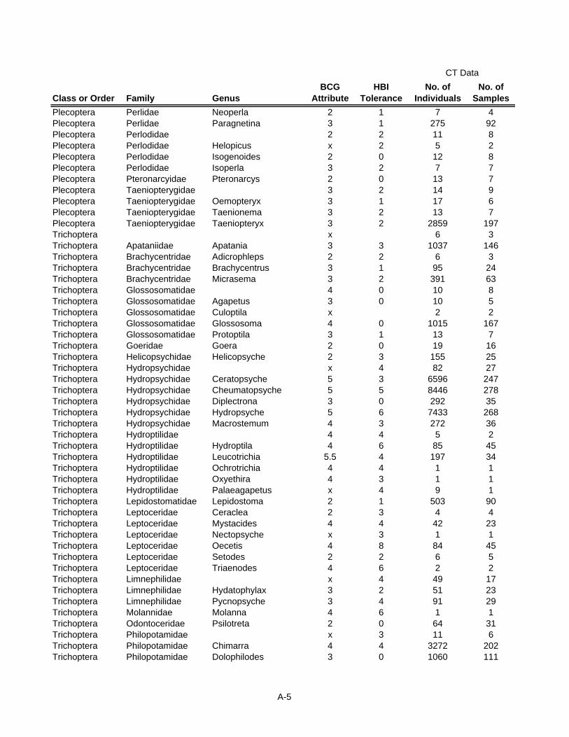
Class or Order Family GenusBCG
AttributeHBI
ToleranceNo. of
IndividualsNo. of
Samples
CT Data
Plecoptera Perlidae Neoperla 2 1 7 4Plecoptera Perlidae Paragnetina 3 1 275 92Plecoptera Perlodidae 2 2 11 8Plecoptera Perlodidae Helopicus x 2 5 2Plecoptera Perlodidae Isogenoides 2 0 12 8Plecoptera Perlodidae Isoperla 3 2 7 7Plecoptera Pteronarcyidae Pteronarcys 2 0 13 7Plecoptera Taeniopterygidae 3 2 14 9Plecoptera Taeniopterygidae Oemopteryx 3 1 17 6Plecoptera Taeniopterygidae Taenionema 3 2 13 7Plecoptera Taeniopterygidae Taeniopteryx 3 2 2859 197Trichoptera x 6 3Trichoptera Apataniidae Apatania 3 3 1037 146Trichoptera Brachycentridae Adicrophleps 2 2 6 3Trichoptera Brachycentridae Brachycentrus 3 1 95 24Trichoptera Brachycentridae Micrasema 3 2 391 63Trichoptera Glossosomatidae 4 0 10 8Trichoptera Glossosomatidae Agapetus 3 0 10 5Trichoptera Glossosomatidae Culoptila x 2 2Trichoptera Glossosomatidae Glossosoma 4 0 1015 167Trichoptera Glossosomatidae Protoptila 3 1 13 7Trichoptera Goeridae Goera 2 0 19 16Trichoptera Helicopsychidae Helicopsyche 2 3 155 25Trichoptera Hydropsychidae x 4 82 27Trichoptera Hydropsychidae Ceratopsyche 5 3 6596 247Trichoptera Hydropsychidae Cheumatopsyche 5 5 8446 278Trichoptera Hydropsychidae Diplectrona 3 0 292 35Trichoptera Hydropsychidae Hydropsyche 5 6 7433 268Trichoptera Hydropsychidae Macrostemum 4 3 272 36Trichoptera Hydroptilidae 4 4 5 2Trichoptera Hydroptilidae Hydroptila 4 6 85 45Trichoptera Hydroptilidae Leucotrichia 5.5 4 197 34Trichoptera Hydroptilidae Ochrotrichia 4 4 1 1Trichoptera Hydroptilidae Oxyethira 4 3 1 1Trichoptera Hydroptilidae Palaeagapetus x 4 9 1Trichoptera Lepidostomatidae Lepidostoma 2 1 503 90Trichoptera Leptoceridae Ceraclea 2 3 4 4Trichoptera Leptoceridae Mystacides 4 4 42 23Trichoptera Leptoceridae Nectopsyche x 3 1 1Trichoptera Leptoceridae Oecetis 4 8 84 45Trichoptera Leptoceridae Setodes 2 2 6 5Trichoptera Leptoceridae Triaenodes 4 6 2 2Trichoptera Limnephilidae x 4 49 17Trichoptera Limnephilidae Hydatophylax 3 2 51 23Trichoptera Limnephilidae Pycnopsyche 3 4 91 29Trichoptera Molannidae Molanna 4 6 1 1Trichoptera Odontoceridae Psilotreta 2 0 64 31Trichoptera Philopotamidae x 3 11 6Trichoptera Philopotamidae Chimarra 4 4 3272 202Trichoptera Philopotamidae Dolophilodes 3 0 1060 111
A-5
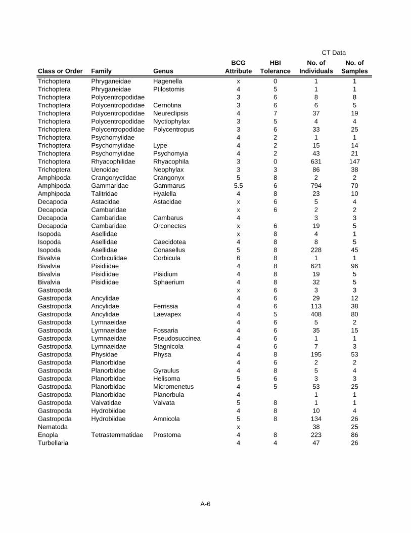
Class or Order Family GenusBCG
AttributeHBI
ToleranceNo. of
IndividualsNo. of
Samples
CT Data
Trichoptera Phryganeidae Hagenella x 0 1 1Trichoptera Phryganeidae Ptilostomis 4 5 1 1Trichoptera Polycentropodidae 3 6 8 8Trichoptera Polycentropodidae Cernotina 3 6 6 5Trichoptera Polycentropodidae Neureclipsis 4 7 37 19Trichoptera Polycentropodidae Nyctiophylax 3 5 4 4Trichoptera Polycentropodidae Polycentropus 3 6 33 25Trichoptera Psychomyiidae 4 2 1 1Trichoptera Psychomyiidae Lype 4 2 15 14Trichoptera Psychomyiidae Psychomyia 4 2 43 21Trichoptera Rhyacophilidae Rhyacophila 3 0 631 147Trichoptera Uenoidae Neophylax 3 3 86 38Amphipoda Crangonyctidae Crangonyx 5 8 2 2Amphipoda Gammaridae Gammarus 5.5 6 794 70Amphipoda Talitridae Hyalella 4 8 23 10Decapoda Astacidae Astacidae x 6 5 4Decapoda Cambaridae x 6 2 2Decapoda Cambaridae Cambarus 4 3 3Decapoda Cambaridae Orconectes x 6 19 5Isopoda Asellidae x 8 4 1Isopoda Asellidae Caecidotea 4 8 8 5Isopoda Asellidae Conasellus 5 8 228 45Bivalvia Corbiculidae Corbicula 6 8 1 1Bivalvia Pisidiidae 4 8 621 96Bivalvia Pisidiidae Pisidium 4 8 19 5Bivalvia Pisidiidae Sphaerium 4 8 32 5Gastropoda x 6 3 3Gastropoda Ancylidae 4 6 29 12Gastropoda Ancylidae Ferrissia 4 6 113 38Gastropoda Ancylidae Laevapex 4 5 408 80Gastropoda Lymnaeidae 4 6 5 2Gastropoda Lymnaeidae Fossaria 4 6 35 15Gastropoda Lymnaeidae Pseudosuccinea 4 6 1 1Gastropoda Lymnaeidae Stagnicola 4 6 7 3Gastropoda Physidae Physa 4 8 195 53Gastropoda Planorbidae 4 6 2 2Gastropoda Planorbidae Gyraulus 4 8 5 4Gastropoda Planorbidae Helisoma 5 6 3 3Gastropoda Planorbidae Micromenetus 4 5 53 25Gastropoda Planorbidae Planorbula 4 1 1Gastropoda Valvatidae Valvata 5 8 1 1Gastropoda Hydrobiidae 4 8 10 4Gastropoda Hydrobiidae Amnicola 5 8 134 26Nematoda x 38 25Enopla Tetrastemmatidae Prostoma 4 8 223 86Turbellaria 4 4 47 26
A-6

APPENDIX B
BIOLOGICAL DATA AND BCG LEVEL ASSIGNMENTS

Stream name date EP GH MB JG BJ median mean NominalHockanum Brook 10/31/1996 4.2 3.5 3.5 3.5 3.7333 3East Branch Byram River 10/03/2002 3.8 4.2 3.8 3.2 3.8 3.75 3East Branch Byram River 10/03/2002 3.8 4.2 3.5 3.8 3.8333 3Hockanum River 10/26/1998 5.5 5.5 5.8 5.5 5.2 5.5 5.5 5Mad River 11/14/1996 5.8 6.5 6.5 6.5 6.2 6.5 6.3 6Mattabesset River 10/16/1996 5.5 5.8 5.8 5.5 5.5 5.5 5.62 5Mill River 11/13/1997 4.2 4.2 4.2 4.8 3.8 4.2 4.24 4Mill River 10/14/1997 3.8 3.5 3.5 3.5 3.6 3Branford River 10/17/1997 4.2 3.8 4.5 4.5 4.8 4.5 4.36 4Naugatuck River 11/05/1996 5.5 5.2 5.2 5.5 5.35 5.35 5Noroton River 10/10/2000 5.5 5.8 5.8 6.2 5.8 5.8 5.82 5Norwalk River 10/30/1997 5.5 5.2 5.5 5.5 5.5 5.5 5.44 5Norwalk River 10/28/1997 5.2 5.2 5.2 5.5 5.2 5.2 5.26 5Byram River 10/20/1997 5.8 5.8 5.8 5.5 5.5 5.8 5.68 5Pattaconk Brook 10/29/1998 3.5 3.5 3.5 3.2 3.2 3.5 3.38 3Pequabuck River 10/01/1998 5.2 5.2 5.2 4.8 5.2 5.2 5.12 5Pequabuck River 10/01/1998 5.5 5.8 5.8 5.8 5.8 5.8 5.74 5Pequabuck River 10/02/1998 5.8 5.8 5.8 5.8 5.8 5Quinnipiac River 10/14/1997 5.5 6.2 5.2 5.8 5.5 5.5 5.64 5Rippowam River 10/31/1997 5.5 5.5 5.5 5.5 5.5 5.5 5.5 5Salmon Brook 10/19/1998 4.5 3.5 3.5 3.8 4.2 3.8 3.9 3Salmon River 10/27/1998 2.2 2.5 2.5 2.5 2.8 2.5 2.5 2Sandy Brook 10/21/1998 2.5 2.5 2.8 2.5 2.8 2.5 2.62 2Scantic River 10/22/1998 4.8 5.2 4.5 4.8 4.8 4.825 4Shetucket River 10/28/1999 4.8 5.2 4.8 4.8 4.8 4.8 4.88 4Still River 10/24/2000 6.2 6.2 6.2 6.5 6.2 6.275 6West Branch Naugatuck Rive 11/05/1996 4.2 3.5 4.2 4.5 4.2 4.2 4.12 4Willimantic River 10/14/1999 3.5 3.8 4.2 3.5 3.5 3.5 3.7 3Willimantic River 10/03/2000 5.5 5.8 5.8 6.2 5.8 5.8 5.82 5Mount Hope River 10/26/1999 3.5 3.2 3.5 3.5 3.4 3Moosup River 10/28/1999 3.5 3.2 3.5 3.5 3.4 3Blackwell Brook 10/22/1999 3.8 3.8 3.8 3.5 3.5 3.8 3.68 3Broad Brook 10/06/1999 3.8 4.5 4.2 3.8 4.2 4.2 4.1 4Merrick Brook 10/07/1999 2.8 2.8 2.8 2.5 2.8 2.8 2.74 2Quinebaug River 10/27/1999 4.5 4.5 4.2 4.5 4.8 4.5 4.5 4Shunock River 10/07/2003 3.8 4.2 3.5 3.5 4.2 3.8 3.84 3Seth Williams Brook 10/19/2000 5.5 5.5 5.5 5.5 5.5 5.5 5.5 5Quaker Brook 10/23/2000 3.5 3.2 3.5 3.2 3.2 3.2 3.32 3Sages Ravine Brook 10/21/2002 2.5 2.5 2.5 2.5 2.5 2Furnace Brook 10/13/1999 4.2 4.5 5.2 5.2 4.8 4.8 4.78 4East Branch Salmon Brook 11/01/2004 2.5 2.2 1.8 2.2 2.5 2.2 2.24 2Beach Brook 11/01/2004 2.5 2.5 2.8 2.5 2.5 2.575 2Housatonic River 10/27/2004 3.5 3.8 3.2 3.5 3.5 3Crooked Brook 10/27/2004 3.8 3.5 3.8 3.5 3.8 3.8 3.68 3Clark Creek 10/28/2004 3.5 3.2 3.5 3.2 3.2 3.2 3.32 3Hammonasset River 10/21/1997 3.2 2.8 2.8 2.8 3.2 2.8 2.96 2Sympaug Brook 10/17/2000 5.5 5.8 5.5 5.8 6.2 5.8 5.6857 5Mountain Brook 10/28/2002 2.8 2.8 2.8 2.8 2.88 2
Panel
B-1

APPENDIX C
DESCRIPTIONS OF BCG LEVELS IN CONNECTICUT STREAMS

C-1
Biological Condition Gradient: description of gradient and rules for cold-water streams of Connecticut
Resource Condition Tiers
Biological Condition Characteristics (Effects)
1 Natural or native condition Native structural, functional and taxonomic integrity is preserved; ecosystem function is preserved within the range of natural variability
I Historically documented, sensitive, long-lived, or regionally endemic taxa Long-lived native species of fish-host specialist or long-term brooder mussels such as Brook floater-
Alasmodonta varicosa; Triangle floater- Alasmodonta undulata; Yellow lampmussel- Lampsilis cariosa are present in naturally occurring densities
II Highly Sensitive taxa
The proportion of total richness represented by rare, specialist and vulnerable taxa is high: Plecoptera: Peltoperlidae, Amphinemura, Isogenoides, Neoperla, Pteronarcys, Leuctra; Ephemeroptera: Centroptilum, Heterocloeon, Brachycercus, Drunella, Rhithrogena, Epeorus, Leucrocuta; Trichoptera: Protoptila; Psilotreta, Lepidostoma, Ceraclea; Diptera: Blephariceridae, Stempellina, Limnophila
III Intermediate Sensitive taxa
Densities of Intermediate Sensitive taxa are as naturally occur: Plecoptera: Acroneuria; Ephemeroptera: Ephemerella, Baetisca, Procloeon; Coleoptera: Psephenus Diptera: Rheocricotopus, Stempelinella
IV Taxa of Intermediate tolerance
Densities of intermediate tolerance taxa are as naturally occur: Trichoptera: Diplectrona, Hydroptila, Chimarra, Neureclipsis; Diptera: Tvetenia, Polypedilum ,Microtendipes, Simulium; Coleoptera: Stenelmis;
V Tolerant taxa
Occurrence and densities of Tolerant taxa are as naturally occur: Diptera: Cricotopus, Chironomus, Rheotanytarsus, Dicrotendipes; Non-Insects: Caecidotea, Isopoda, Erpobdellidae, Tubificidae, Glossiphoniidae
VI Non native or intentionally introduced taxa
Non native taxa such as Brown trout, Rainbow trout, Yellow perch, are absent or, if they occur, their presence does not displace native biota or alter native structure and function
VII Physiological condition of long-lived organisms
Anomalies are absent or rare; any that occur are consistent with naturally occurring incidence and characteristics
VIII Ecosystem Function
Rates and characteristics of life history (e.g., reproduction, immigration, mortality, etc.), and materials exchange processes (e.g., production, respiration, nutrient exchange, decomposition, etc.) are comparable to that of “natural” systems
The system is predominantly heterotrophic, sustained by leaf litter inputs from intact riparian areas, with low algal biomass; P/R<1 (Photosynthesis: Respiration ratio)
IX Spatial and temporal extent of detrimental effects
Not applicable- disturbance is limited to natural events such as storms, droughts, fire, earth-flows. A natural flow regime is maintained.
X Ecosystem connectance
Reach is highly connected with groundwater, its floodplain, and riparian zone, and other reaches in the basin, at least annually. Allows for access to habitats and maintenance of seasonal cycles that are necessary for life history requirements, colonization sources, migration and refugia for extreme events.

C-2
2 Minimal changes in structure of the biotic community and minimal changes in ecosystem function Virtually all native taxa are maintained with some changes in biomass and/or abundance; ecosystem functions are fully maintained within the range of natural variability
Whole assemblage and sample Overall taxa richness and density is as naturally occurs RULE 1, 2: Taxa richness is high and subsample density is near target Quantitative Rule 1, 2: Total taxa > (25-30) genera and Total individuals > (50-60%
of target) I Historically documented, sensitive, long-lived, regionally endemic taxa
Rule not defined. II Highly Sensitive taxa
Richness of rare and/or specialist invertebrate taxa is low to moderate though densities may be low .
RULE 3: At least some taxa are present Quantitative Rule 3: Taxa (II) > (3-5)
III Intermediate Sensitive taxa
Richness and abundance of intermediate sensititve taxa is high. Some may have increased due to slightly elevated production
RULE 4: All sensitive taxa (highly sensitive + intermediate sensitive): comprise half
or more of all taxa RULE 5 : All sensitive individuals: comprise nearly half or more of all organisms Quantitative Rule 4: Taxa (II + III) > (45 – 55%) of all taxa Quantitative Rule 5: Individuals (II + III) > (30-40%)
IV Taxa of Intermediate tolerance
May be slight increases in densities of macroinvertebrate taxa RULE: None
V Tolerant taxa (also includes taxa considered highly tolerant)
Occurrence and densities of Tolerant taxa are as naturally occur. Typically present but a very small fraction of organisms.
RULE 6: Tolerant individuals (tolerant + highly tolerant) comprise a small fraction or less of all organisms
Quantitative Rule 6: Individuals (V) < (10-15%) VI-IX Non-native taxa; Physiological condition; Ecosystem Function; Spatial and temporal extent
Not addressed for macroinvertebrates X Ecosystem connectance
Connectance on a local scale (floodplain, tributaries) remains good but dams and other flow obstructions downstream impede migration of fish and mussels (eels, salmonids, migration-dependent unionids)
COMBINATORIAL RULE
To be considered Tier 2, rules 1 - 4 must apply; combined with AND, and Rule OR Rule 6.
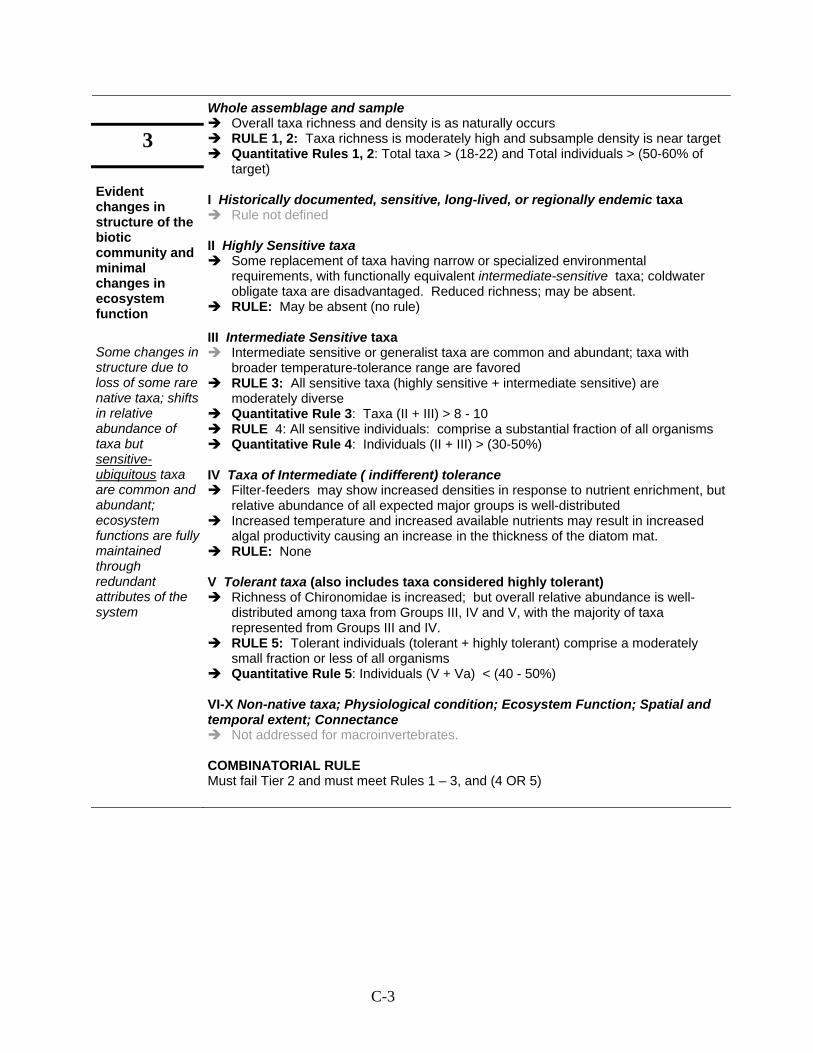
C-3
3 Evident changes in structure of the biotic community and minimal changes in ecosystem function Some changes in structure due to loss of some rare native taxa; shifts in relative abundance of taxa but sensitive-ubiquitous taxa are common and abundant; ecosystem functions are fully maintained through redundant attributes of the system
Whole assemblage and sample Overall taxa richness and density is as naturally occurs RULE 1, 2: Taxa richness is moderately high and subsample density is near target Quantitative Rules 1, 2: Total taxa > (18-22) and Total individuals > (50-60% of
target) I Historically documented, sensitive, long-lived, or regionally endemic taxa
Rule not defined II Highly Sensitive taxa
Some replacement of taxa having narrow or specialized environmental requirements, with functionally equivalent intermediate-sensitive taxa; coldwater obligate taxa are disadvantaged. Reduced richness; may be absent.
RULE: May be absent (no rule) III Intermediate Sensitive taxa
Intermediate sensitive or generalist taxa are common and abundant; taxa with broader temperature-tolerance range are favored
RULE 3: All sensitive taxa (highly sensitive + intermediate sensitive) are moderately diverse
Quantitative Rule 3: Taxa (II + III) > 8 - 10 RULE 4: All sensitive individuals: comprise a substantial fraction of all organisms Quantitative Rule 4: Individuals (II + III) > (30-50%)
IV Taxa of Intermediate ( indifferent) tolerance
Filter-feeders may show increased densities in response to nutrient enrichment, but relative abundance of all expected major groups is well-distributed
Increased temperature and increased available nutrients may result in increased algal productivity causing an increase in the thickness of the diatom mat.
RULE: None
V Tolerant taxa (also includes taxa considered highly tolerant) Richness of Chironomidae is increased; but overall relative abundance is well-
distributed among taxa from Groups III, IV and V, with the majority of taxa represented from Groups III and IV.
RULE 5: Tolerant individuals (tolerant + highly tolerant) comprise a moderately small fraction or less of all organisms
Quantitative Rule 5: Individuals (V + Va) < (40 - 50%) VI-X Non-native taxa; Physiological condition; Ecosystem Function; Spatial and temporal extent; Connectance
Not addressed for macroinvertebrates. COMBINATORIAL RULE Must fail Tier 2 and must meet Rules 1 – 3, and (4 OR 5)
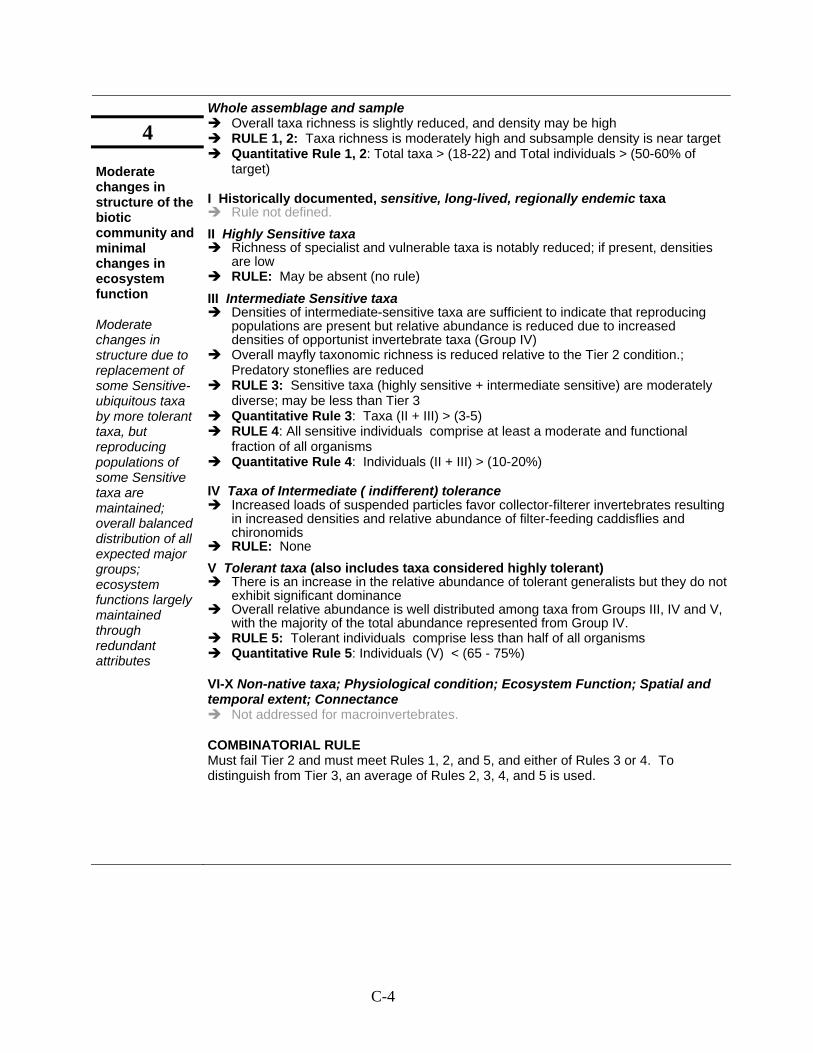
C-4
4 Moderate changes in structure of the biotic community and minimal changes in ecosystem function Moderate changes in structure due to replacement of some Sensitive-ubiquitous taxa by more tolerant taxa, but reproducing populations of some Sensitive taxa are maintained; overall balanced distribution of all expected major groups; ecosystem functions largely maintained through redundant attributes
Whole assemblage and sample Overall taxa richness is slightly reduced, and density may be high RULE 1, 2: Taxa richness is moderately high and subsample density is near target Quantitative Rule 1, 2: Total taxa > (18-22) and Total individuals > (50-60% of
target) I Historically documented, sensitive, long-lived, regionally endemic taxa
Rule not defined. II Highly Sensitive taxa
Richness of specialist and vulnerable taxa is notably reduced; if present, densities are low
RULE: May be absent (no rule)
III Intermediate Sensitive taxa Densities of intermediate-sensitive taxa are sufficient to indicate that reproducing
populations are present but relative abundance is reduced due to increased densities of opportunist invertebrate taxa (Group IV)
Overall mayfly taxonomic richness is reduced relative to the Tier 2 condition.; Predatory stoneflies are reduced
RULE 3: Sensitive taxa (highly sensitive + intermediate sensitive) are moderately diverse; may be less than Tier 3
Quantitative Rule 3: Taxa (II + III) > (3-5) RULE 4: All sensitive individuals comprise at least a moderate and functional
fraction of all organisms Quantitative Rule 4: Individuals (II + III) > (10-20%)
IV Taxa of Intermediate ( indifferent) tolerance
Increased loads of suspended particles favor collector-filterer invertebrates resulting in increased densities and relative abundance of filter-feeding caddisflies and chironomids
RULE: None V Tolerant taxa (also includes taxa considered highly tolerant)
There is an increase in the relative abundance of tolerant generalists but they do not exhibit significant dominance
Overall relative abundance is well distributed among taxa from Groups III, IV and V, with the majority of the total abundance represented from Group IV.
RULE 5: Tolerant individuals comprise less than half of all organisms Quantitative Rule 5: Individuals (V) < (65 - 75%)
VI-X Non-native taxa; Physiological condition; Ecosystem Function; Spatial and temporal extent; Connectance
Not addressed for macroinvertebrates. COMBINATORIAL RULE Must fail Tier 2 and must meet Rules 1, 2, and 5, and either of Rules 3 or 4. To distinguish from Tier 3, an average of Rules 2, 3, 4, and 5 is used.
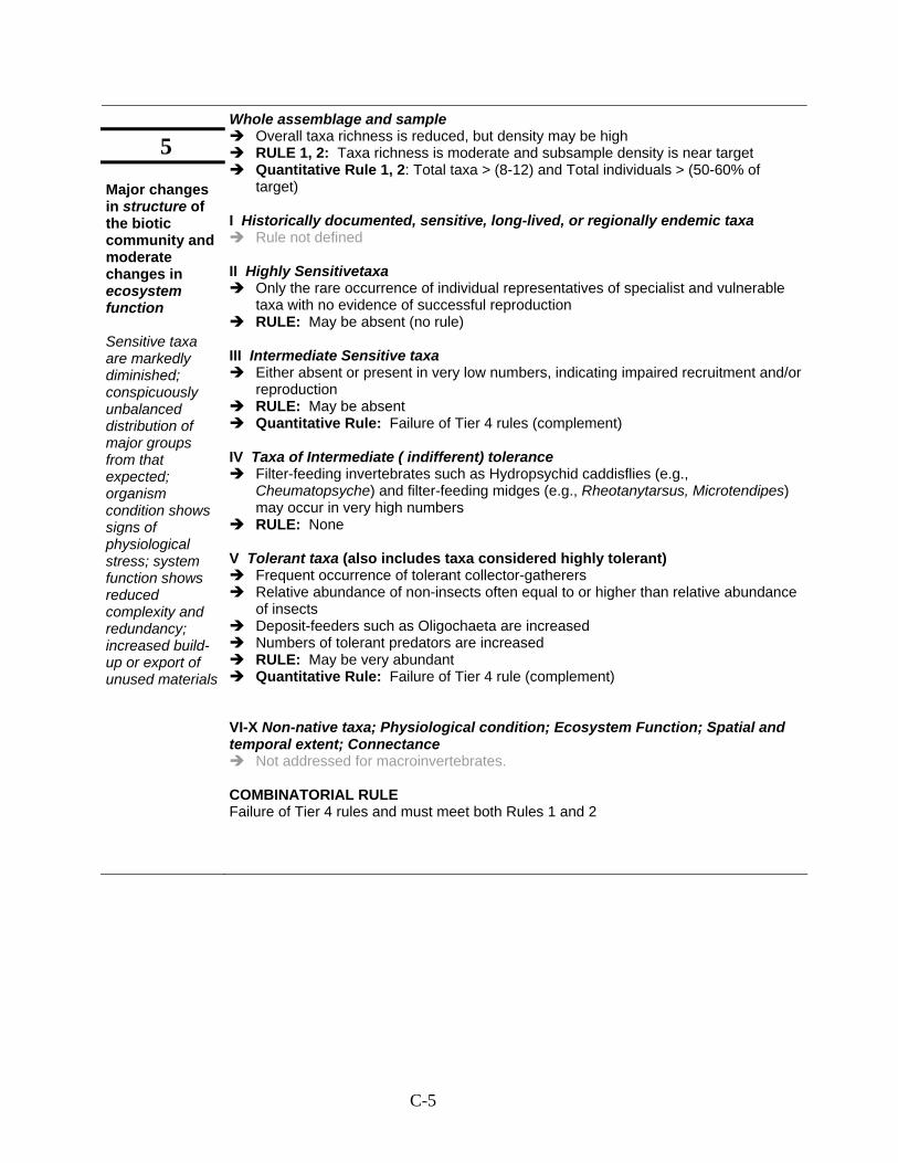
C-5
5 Major changes in structure of the biotic community and moderate changes in ecosystem function Sensitive taxa are markedly diminished; conspicuously unbalanced distribution of major groups from that expected; organism condition shows signs of physiological stress; system function shows reduced complexity and redundancy; increased build-up or export of unused materials
Whole assemblage and sample Overall taxa richness is reduced, but density may be high RULE 1, 2: Taxa richness is moderate and subsample density is near target Quantitative Rule 1, 2: Total taxa > (8-12) and Total individuals > (50-60% of
target) I Historically documented, sensitive, long-lived, or regionally endemic taxa
Rule not defined II Highly Sensitivetaxa
Only the rare occurrence of individual representatives of specialist and vulnerable taxa with no evidence of successful reproduction
RULE: May be absent (no rule) III Intermediate Sensitive taxa
Either absent or present in very low numbers, indicating impaired recruitment and/or reproduction
RULE: May be absent Quantitative Rule: Failure of Tier 4 rules (complement)
IV Taxa of Intermediate ( indifferent) tolerance
Filter-feeding invertebrates such as Hydropsychid caddisflies (e.g., Cheumatopsyche) and filter-feeding midges (e.g., Rheotanytarsus, Microtendipes) may occur in very high numbers
RULE: None V Tolerant taxa (also includes taxa considered highly tolerant)
Frequent occurrence of tolerant collector-gatherers Relative abundance of non-insects often equal to or higher than relative abundance
of insects Deposit-feeders such as Oligochaeta are increased Numbers of tolerant predators are increased RULE: May be very abundant Quantitative Rule: Failure of Tier 4 rule (complement)
VI-X Non-native taxa; Physiological condition; Ecosystem Function; Spatial and temporal extent; Connectance
Not addressed for macroinvertebrates. COMBINATORIAL RULE Failure of Tier 4 rules and must meet both Rules 1 and 2
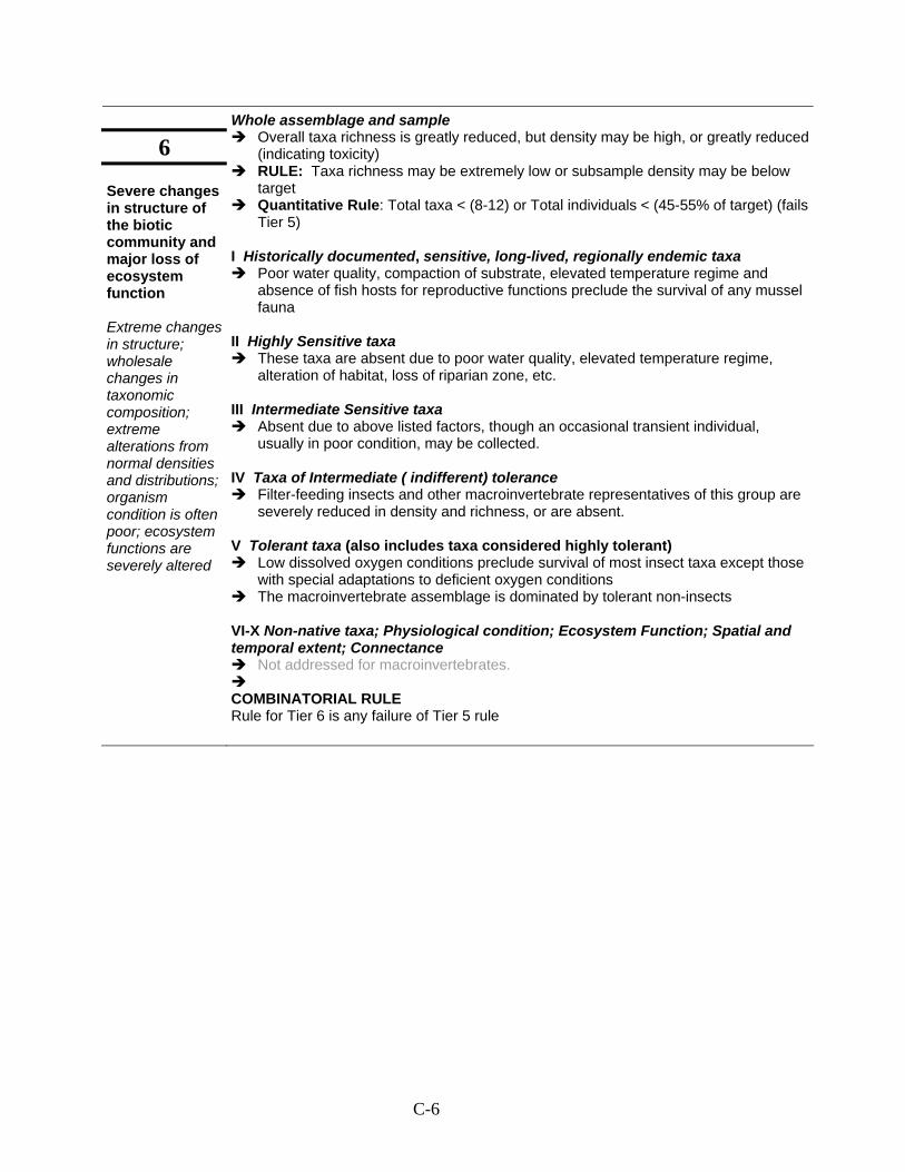
C-6
6 Severe changes in structure of the biotic community and major loss of ecosystem function Extreme changes in structure; wholesale changes in taxonomic composition; extreme alterations from normal densities and distributions; organism condition is often poor; ecosystem functions are severely altered
Whole assemblage and sample Overall taxa richness is greatly reduced, but density may be high, or greatly reduced
(indicating toxicity) RULE: Taxa richness may be extremely low or subsample density may be below
target Quantitative Rule: Total taxa < (8-12) or Total individuals < (45-55% of target) (fails
Tier 5) I Historically documented, sensitive, long-lived, regionally endemic taxa
Poor water quality, compaction of substrate, elevated temperature regime and absence of fish hosts for reproductive functions preclude the survival of any mussel fauna
II Highly Sensitive taxa
These taxa are absent due to poor water quality, elevated temperature regime, alteration of habitat, loss of riparian zone, etc.
III Intermediate Sensitive taxa
Absent due to above listed factors, though an occasional transient individual, usually in poor condition, may be collected.
IV Taxa of Intermediate ( indifferent) tolerance
Filter-feeding insects and other macroinvertebrate representatives of this group are severely reduced in density and richness, or are absent.
V Tolerant taxa (also includes taxa considered highly tolerant)
Low dissolved oxygen conditions preclude survival of most insect taxa except those with special adaptations to deficient oxygen conditions
The macroinvertebrate assemblage is dominated by tolerant non-insects VI-X Non-native taxa; Physiological condition; Ecosystem Function; Spatial and temporal extent; Connectance
Not addressed for macroinvertebrates.
COMBINATORIAL RULE Rule for Tier 6 is any failure of Tier 5 rule

APPENDIX D
METRIC STATISTICS
D-1
Appendix D
Metric Statistics Trend: Direction of metric response with increasing stress. The trends for unresponsive metrics were left blank.
Incr = increasing metric values with increasing stress. Decr = decreasing metric values with increasing stress.
DE: Discrimination Efficiency = the percentage of degraded samples lower or higher than the quartile of the reference samples, in the direction of the trend. This appendix considers calibration data only. CVref: Coefficient of Variability = the standard deviation of reference metric values over the mean of the values, expressed as a percentage.

D-2
Metric Name Metric Code Trend DE CVref
Richness Total Taxa TotalTax Decr 100 22.2 Insect Taxa InsecTax Decr 100 23.6 Non-Insect Taxa Percent NonInsPT Incr 83.3 83.1 EPT Taxa EPTTax Decr 100 22.9 Ephemeroptera Taxa EphemTax Decr 100 33.0 Ephemeroptera Taxa (adjusted for watershed area) adjEphemTax Decr 100 18.7 Plecoptera Taxa PlecoTax Decr 100 45.5 Trichoptera Taxa TrichTax Decr 83.3 33.8 Diptera Taxa DipTax Decr 41.7 55.0 Midge Taxa ChiroTax Decr 41.7 68.5 Orthocladiinae Taxa OrthoTax 73.2 Tanytarsini Taxa TanytTax 94.9 Coleoptera Taxa ColeoTax Decr 100 41.2 Crustacea & Mollusca Taxa CrMolTax 8.3 101.0 Oligochaeta Taxa OligoTax 135.6 Composition % EPT EPTPct Incr 50.0 28.2 % EPT excluding Hydropsychidae and Baetidae EPTnHBpct Decr 100 37.3 % EPT excluding Hydropsychidae and Baetidae (adjusted for watershed area) adj%SEPT Decr 100 31.3
% Ephemeroptera EphemPct Decr 66.7 71.4 % Plecoptera PlecoPct Decr 100 84.3 % Trichoptera TrichPct Incr 100 53.3 % Baetidae:Ephemeroptera Baet2EphPct 16.7 217.9 % Hydropsychidae:EPT Hyd2EPTPct Incr 100 74.6 % Hydropsychidae:Trichoptera Hyd2TriPct Incr 100 52.8 % Diptera DipPct 116.2 % Midge ChiroPct Decr 41.7 135.5 % Non-Insect NonInPct Incr 50.0 160.2 % Amphipoda AmphPct 33.3 % Coleoptera ColeoPct Decr 91.7 68.5 Cricotopus&Chironomus/Chironomidae CrCh2ChiPct 33.3 361.8 % Bivalvia BivalPct 8.3 212.1 % Crustacea & Mollusca CrMolPct Incr 41.7 237.9 % Gastropoda GastrPct Incr 41.7 270.7 % Isopoda IsoPct 25.0 % Odonata OdonPct 8.3 126.9 % Oligochaeta OligoPct 16.7 277.2 % Orthocladiinae:Midges Orth2ChiPct Incr 41.7 70.3 % Tanytarsini TanytPct 179.6 % Tanytarsini:Midges Tnyt2ChiPct 33.3 116.4 Evenness Shannon-Weiner Index (base e) Shan_e Decr 100 13.7 Evenness Evenness Decr 91.7 14.5 Margoleff's Diversity D_Mg Decr 100 23.8 Simpson's Index D Incr 100 49.3
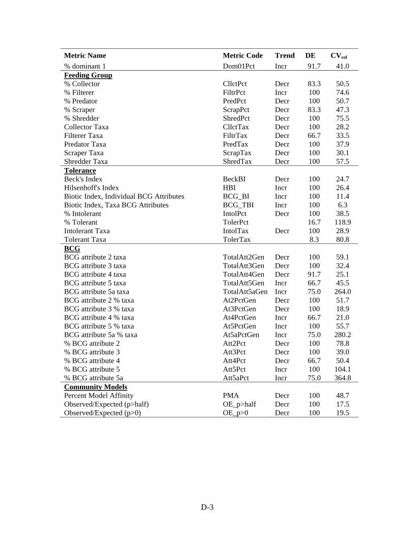
D-3
Metric Name Metric Code Trend DE CVref % dominant 1 Dom01Pct Incr 91.7 41.0 Feeding Group % Collector CllctPct Decr 83.3 50.5 % Filterer FiltrPct Incr 100 74.6 % Predator PredPct Decr 100 50.7 % Scraper ScrapPct Decr 83.3 47.3 % Shredder ShredPct Decr 100 75.5 Collector Taxa CllctTax Decr 100 28.2 Filterer Taxa FiltrTax Decr 66.7 33.5 Predator Taxa PredTax Decr 100 37.9 Scraper Taxa ScrapTax Decr 100 30.1 Shredder Taxa ShredTax Decr 100 57.5 Tolerance Beck's Index BeckBI Decr 100 24.7 Hilsenhoff's Index HBI Incr 100 26.4 Biotic Index, Individual BCG Attributes BCG_BI Incr 100 11.4 Biotic Index, Taxa BCG Attributes BCG_TBI Incr 100 6.3 % Intolerant IntolPct Decr 100 38.5 % Tolerant TolerPct 16.7 118.9 Intolerant Taxa IntolTax Decr 100 28.9 Tolerant Taxa TolerTax 8.3 80.8 BCG BCG attribute 2 taxa TotalAtt2Gen Decr 100 59.1 BCG attribute 3 taxa TotalAtt3Gen Decr 100 32.4 BCG attribute 4 taxa TotalAtt4Gen Decr 91.7 25.1 BCG attribute 5 taxa TotalAtt5Gen Incr 66.7 45.5 BCG attribute 5a taxa TotalAtt5aGen Incr 75.0 264.0 BCG attribute 2 % taxa At2PctGen Decr 100 51.7 BCG attribute 3 % taxa At3PctGen Decr 100 18.9 BCG attribute 4 % taxa At4PctGen Incr 66.7 21.0 BCG attribute 5 % taxa At5PctGen Incr 100 55.7 BCG attribute 5a % taxa At5aPctGen Incr 75.0 280.2 % BCG attribute 2 Att2Pct Decr 100 78.8 % BCG attribute 3 Att3Pct Decr 100 39.0 % BCG attribute 4 Att4Pct Decr 66.7 50.4 % BCG attribute 5 Att5Pct Incr 100 104.1 % BCG attribute 5a Att5aPct Incr 75.0 364.8 Community Models Percent Model Affinity PMA Decr 100 48.7 Observed/Expected (p>half) OE_p>half Decr 100 17.5 Observed/Expected (p>0) OE_p>0 Decr 100 19.5