Calibration Estimation of Semiparametric Copula...
50
Calibration Estimation of Semiparametric Copula Models with Data Missing at Random Shigeyuki Hamori 1 Kaiji Motegi 1 Zheng Zhang 2 1 Kobe University 2 Renmin University of China Econometrics Workshop Keio University July 10, 2018 Hamori, Motegi & Zhang (Kobe & RUC) Copula Models with Data MAR July 10, 2018 1 / 50
Transcript of Calibration Estimation of Semiparametric Copula...

Calibration Estimation of SemiparametricCopula Models with Data Missing at Random
Shigeyuki Hamori1 Kaiji Motegi1 Zheng Zhang2
1Kobe University2Renmin University of China
Econometrics WorkshopKeio University
July 10, 2018
Hamori, Motegi & Zhang (Kobe & RUC) Copula Models with Data MAR July 10, 2018 1 / 50
Introduction
Copula
Model
Treatment
Effect
Data
Missing
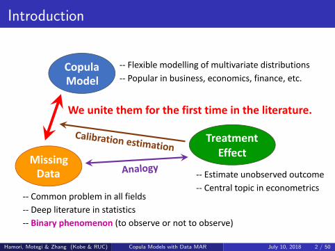
-- Flexible modelling of multivariate distributions
-- Popular in business, economics, finance, etc.
-- Common problem in all fields
-- Deep literature in statistics
-- Central topic in econometrics
-- Estimate unobserved outcome
We unite them for the first time in the literature.
-- Binary phenomenon (to observe or not to observe)
Hamori, Motegi & Zhang (Kobe & RUC) Copula Models with Data MAR July 10, 2018 2 / 50
Introduction
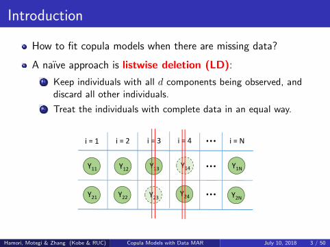
How to fit copula models when there are missing data?
A naıve approach is listwise deletion (LD):
1 Keep individuals with all d components being observed, anddiscard all other individuals.
2 Treat the individuals with complete data in an equal way.
Y2N
…
i = 1 i = 3i = 2 i = 4 i = N…
Y11
Y21
Y12
Y22
Y13
Y23
Y14
Y24
Y1N
…
Hamori, Motegi & Zhang (Kobe & RUC) Copula Models with Data MAR July 10, 2018 3 / 50

Introduction
LD leads to a consistent estimator for the copula parameter ofinterest if the missing mechanism is missing completely atrandom (MCAR).
LD leads to an inconsistent estimator if the missing mechanismis missing at random (MAR).
Under MAR, target variables Yi = [Y1i, . . . , Ydi]⊤ and their
missing status are independent of each other given observedcovariates Xi = [X1i, . . . , Xmi]
⊤.
LD treats individuals with complete data all equally, and it doesnot use the information of Xi. That can cause substantial biasunder MAR.
Hamori, Motegi & Zhang (Kobe & RUC) Copula Models with Data MAR July 10, 2018 4 / 50
Introduction
How to obtain a consistent estimator for the copula parameterwhen the missing mechanism is MAR?
As is well known in the literature of missing data and averagetreatment effects, a key step is the estimation of propensityscore function (i.e. conditional probability of observing datagiven covariates).
Direct estimation of propensity score is notoriously challenging,whether it is performed parametrically or nonparametrically.
Parametric approaches are haunted by misspecificationproblems, while nonparametric approaches often lack stability.
Hamori, Motegi & Zhang (Kobe & RUC) Copula Models with Data MAR July 10, 2018 5 / 50

Introduction
Chan, Yam, and Zhang (2016, JRSS-B) propose an alternativeapproach called calibration estimation in the literature ofaverage treatment effects.
The calibration estimator is derived by balancing covariatesamong treatment, control, and whole groups. It does notrequire a direct estimation of propensity score.
We apply the calibration estimation to a missing data problemfor the first time in the literature.
Hamori, Motegi & Zhang (Kobe & RUC) Copula Models with Data MAR July 10, 2018 6 / 50
Introduction
The calibration estimator for the copula parameter satisfiesconsistency and asymptotic normality under someassumptions including i.i.d. data and the MAR condition.
We also derive a consistent estimator for the asymptoticcovariance matrix.
We perform Monte Carlo simulations. Our simulation resultsindicate that the calibration estimator dominates listwisedeletion, parametric approach, and nonparametric approach.
Hamori, Motegi & Zhang (Kobe & RUC) Copula Models with Data MAR July 10, 2018 7 / 50
Table of Contents
1) Introduction
2) Review of Copula Models
3) Review of Missing Data
4) Set-up of Main Problem
5) Theory of Calibration Estimation
6) Monte Carlo Simulations
7) Conclusions
Hamori, Motegi & Zhang (Kobe & RUC) Copula Models with Data MAR July 10, 2018 8 / 50
Review of Copula Models
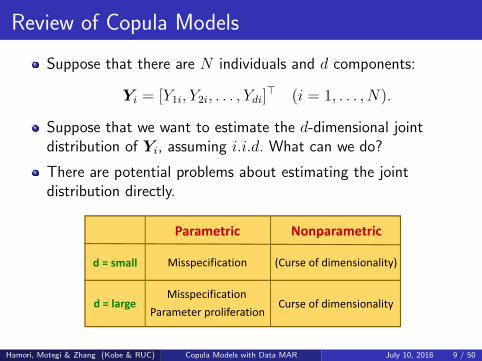
Suppose that there are N individuals and d components:
Yi = [Y1i, Y2i, . . . , Ydi]⊤ (i = 1, . . . , N).
Suppose that we want to estimate the d-dimensional jointdistribution of Yi, assuming i.i.d. What can we do?
There are potential problems about estimating the jointdistribution directly.
Parametric Nonparametric
d = large
d = small Misspecification
MisspecificationCurse of dimensionality
(Curse of dimensionality)
Parameter proliferation
Hamori, Motegi & Zhang (Kobe & RUC) Copula Models with Data MAR July 10, 2018 9 / 50

Review of Copula Models
Copula models accomplish flexible specification with a smallnumber of parameters.
Copula models follow a two-step procedure.
Step 1: Model the marginal distribution of each of the dcomponents separately.
Step 2: Combine the d marginal distributions to recover a jointdistribution.
Step 2
Nonparametric
Parametric
Parametric
Name of model
Parametric copula model
Semiparametric copula model
Nonparametric copula model
(Target of our paper)
Step 1
Parametric
Nonparametric
Nonparametric
Hamori, Motegi & Zhang (Kobe & RUC) Copula Models with Data MAR July 10, 2018 10 / 50
Review of Copula Models
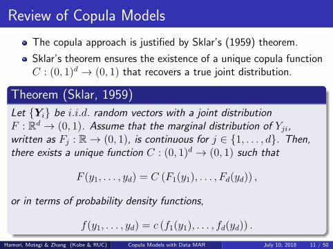
The copula approach is justified by Sklar’s (1959) theorem.
Sklar’s theorem ensures the existence of a unique copula functionC : (0, 1)d → (0, 1) that recovers a true joint distribution.
Theorem (Sklar, 1959)
Let {Yi} be i.i.d. random vectors with a joint distributionF : Rd → (0, 1). Assume that the marginal distribution of Yji,written as Fj : R → (0, 1), is continuous for j ∈ {1, . . . , d}. Then,there exists a unique function C : (0, 1)d → (0, 1) such that
F (y1, . . . , yd) = C (F1(y1), . . . , Fd(yd)) ,
or in terms of probability density functions,
f(y1, . . . , yd) = c (f1(y1), . . . , fd(yd)) .
Hamori, Motegi & Zhang (Kobe & RUC) Copula Models with Data MAR July 10, 2018 11 / 50

Review of Copula Models
A well-known example of copula function: bivariate Claytoncopula with a scalar parameter α > 0.
Cumulative distribution function is
C2(u1, u2; α) = (u−α1 + u−α
2 − 1)−1α ,
where u1 = F1(y1) ∈ (0, 1) and u2 = F2(y2) ∈ (0, 1) aremarginal distribution functions of Y1i and Y2i, respectively.
Probability density function is
c2(u1, u2; α) = (1 + α)(u1u2)−α−1(u−α
1 + u−α2 − 1)−
1α−2.
Kendall’s rank correlation coefficient is τ = α/(α + 2).
Larger α implies stronger association between Y1i and Y2i.
Hamori, Motegi & Zhang (Kobe & RUC) Copula Models with Data MAR July 10, 2018 12 / 50
Review of Copula Models
01
10
1
u2
0.5
u1
20
0.50 0
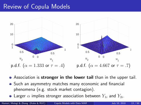
p.d.f. (α = 1.333 or τ = .4)
01
10
1
u2
0.5
u1
20
0.50 0
p.d.f. (α = 4.667 or τ = .7)
Association is stronger in the lower tail than in the upper tail.
Such an asymmetry matches many economic and financialphenomena (e.g. stock market contagion).
Larger α implies stronger association between Y1i and Y2i.
Hamori, Motegi & Zhang (Kobe & RUC) Copula Models with Data MAR July 10, 2018 13 / 50
Review of Missing Data
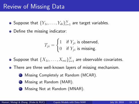
Suppose that {Y1i, . . . , Ydi}Ni=1 are target variables.
Define the missing indicator:
Tji =
{1 if Yji is observed,
0 if Yji is missing.
Suppose that {X1i, . . . , Xmi}Ni=1 are observable covariates.
There are three well-known layers of missing mechanism.
1 Missing Completely at Random (MCAR).
2 Missing at Random (MAR).
3 Missing Not at Random (MNAR).
Hamori, Motegi & Zhang (Kobe & RUC) Copula Models with Data MAR July 10, 2018 14 / 50
Review of Missing Data
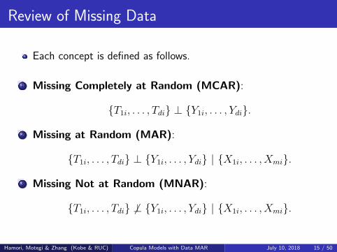
Each concept is defined as follows.
1 Missing Completely at Random (MCAR):
{T1i, . . . , Tdi} ⊥ {Y1i, . . . , Ydi}.
2 Missing at Random (MAR):
{T1i, . . . , Tdi} ⊥ {Y1i, . . . , Ydi} | {X1i, . . . , Xmi}.
3 Missing Not at Random (MNAR):
{T1i, . . . , Tdi} ⊥ {Y1i, . . . , Ydi} | {X1i, . . . , Xmi}.
Hamori, Motegi & Zhang (Kobe & RUC) Copula Models with Data MAR July 10, 2018 15 / 50
Review of Missing Data
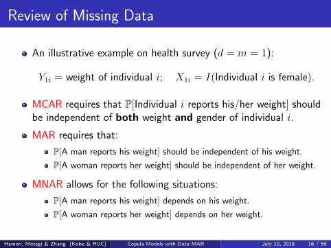
An illustrative example on health survey (d = m = 1):
Y1i = weight of individual i; X1i = I(Individual i is female).
MCAR requires that P[Individual i reports his/her weight] shouldbe independent of both weight and gender of individual i.
MAR requires that:
P[A man reports his weight] should be independent of his weight.
P[A woman reports her weight] should be independent of her weight.
MNAR allows for the following situations:
P[A man reports his weight] depends on his weight.
P[A woman reports her weight] depends on her weight.
Hamori, Motegi & Zhang (Kobe & RUC) Copula Models with Data MAR July 10, 2018 16 / 50
Review of Missing Data
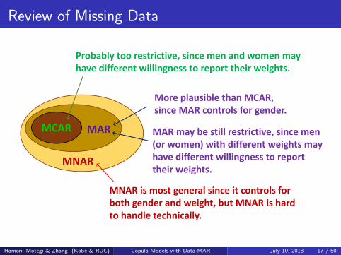
MCAR MAR
MNAR
Probably too restrictive, since men and women may
have different willingness to report their weights.
More plausible than MCAR,
since MAR controls for gender.
MNAR is most general since it controls for
both gender and weight, but MNAR is hard
to handle technically.
MAR may be still restrictive, since men
(or women) with different weights may
have different willingness to report
their weights.
Hamori, Motegi & Zhang (Kobe & RUC) Copula Models with Data MAR July 10, 2018 17 / 50

Review of Missing Data
It is well known that listwise deletion (LD) leads to consistentinference under MCAR.
It is also well known that LD leads to inconsistent inferenceunder MAR.
Correct inference under MAR has been extensively studied sincethe seminal work of Rubin (1976).
The present paper assumes MAR and elaborates the estimationof semiparametric copula models, which has not been done inthe literature.
Hamori, Motegi & Zhang (Kobe & RUC) Copula Models with Data MAR July 10, 2018 18 / 50
Set-up of Main Problem
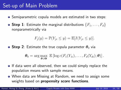
Semiparametric copula models are estimated in two steps:
Step 1: Estimate the marginal distributions {F1, . . . , Fd}nonparametrically via
Fj(y) = P(Yji ≤ y) = E[I(Yji ≤ y)].
Step 2: Estimate the true copula parameter θ0 via
θ0 = argmaxθ∈Θ
E [log c(F1(Y1i), . . . , Fd(Ydi);θ)] .
If data were all observed, then we could simply replace thepopulation means with sample means.
When data are Missing at Random, we need to assign someweights based on propensity score functions.
Hamori, Motegi & Zhang (Kobe & RUC) Copula Models with Data MAR July 10, 2018 19 / 50

Set-up of Main Problem
Define propensity score functions:
πj(x) = P(Tji = 1 |Xi = x), j ∈ {1, . . . , d}.
Define pj(x) = 1/πj(x).
Step 1 is rewritten as
Fj(y) = E[I(Yji ≤ y)] = E[E[I(Yji ≤ y)|Xi]] (∵ LIE)
= E[E[
Tji
πj(Xi)
∣∣∣∣Xi
]× E [I(Yji ≤ y)|Xi]
]= E
[E[
Tji
πj(Xi)× I(Yji ≤ y)
∣∣∣∣Xi
]](∵ MAR)
= E[
Tji
πj(Xi)× I(Yji ≤ y)
](∵ LIE)
= E[Tji × pj(Xi)× I(Yji ≤ y)].
Hamori, Motegi & Zhang (Kobe & RUC) Copula Models with Data MAR July 10, 2018 20 / 50
Set-up of Main Problem
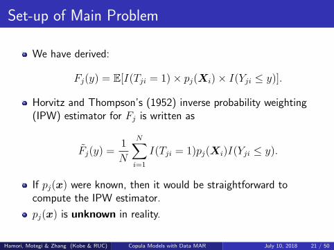
We have derived:
Fj(y) = E[I(Tji = 1)× pj(Xi)× I(Yji ≤ y)].
Horvitz and Thompson’s (1952) inverse probability weighting(IPW) estimator for Fj is written as
Fj(y) =1
N
N∑i=1
I(Tji = 1)pj(Xi)I(Yji ≤ y).
If pj(x) were known, then it would be straightforward tocompute the IPW estimator.
pj(x) is unknown in reality.
Hamori, Motegi & Zhang (Kobe & RUC) Copula Models with Data MAR July 10, 2018 21 / 50
Set-up of Main Problem
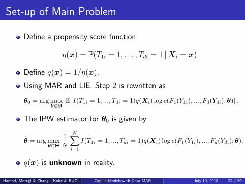
Define a propensity score function:
η(x) = P(T1i = 1, . . . , Tdi = 1 |Xi = x).
Define q(x) = 1/η(x).
Using MAR and LIE, Step 2 is rewritten as
θ0 = argmaxθ∈Θ
E [I(T1i = 1, ..., Tdi = 1)q(Xi) log c(F1(Y1i), ..., Fd(Ydi);θ)] .
The IPW estimator for θ0 is given by
θ = argmaxθ∈Θ
1
N
N∑i=1
I(T1i = 1, ..., Tdi = 1)q(Xi) log c(F1(Y1i), ..., Fd(Ydi);θ).
q(x) is unknown in reality.
Hamori, Motegi & Zhang (Kobe & RUC) Copula Models with Data MAR July 10, 2018 22 / 50

Set-up of Main Problem
Estimation of propensity score functions has been a major issuein the literature of missing data and treatment effects.
Many papers attempt a direct estimation of pj(x) and q(x),either parametrically or nonparametrically.
Parametric approaches: Zhao and Lipsitz (1992), Robins,Rotnitzky, and Zhao (1994), and Bang and Robins (2005).
The parametric approaches are notoriously sensitive tomisspecification (cf. Lawless, Kalbfleisch, and Wild, 1999).
Nonparametric approaches: Hahn (1998), Hirano, Imbens,and Ridder (2003), Imbens, Newey, and Ridder (2005), andChen, Hong, and Tarozzi (2008).
The nonparametric approaches have a notoriously poorperformance in finite sample.
Hamori, Motegi & Zhang (Kobe & RUC) Copula Models with Data MAR July 10, 2018 23 / 50
Theory of Calibration Estimation
In the treatment effect literature, Chan, Yam, and Zhang (2016)propose an alternative approach that bypasses a directestimation of propensity score.
They construct calibration weights by balancing the momentsof observed covariates among treatment, control, and wholegroups.
The present paper applies their method to a missing dataproblem for the first time.
Hamori, Motegi & Zhang (Kobe & RUC) Copula Models with Data MAR July 10, 2018 24 / 50
Theory of Calibration Estimation
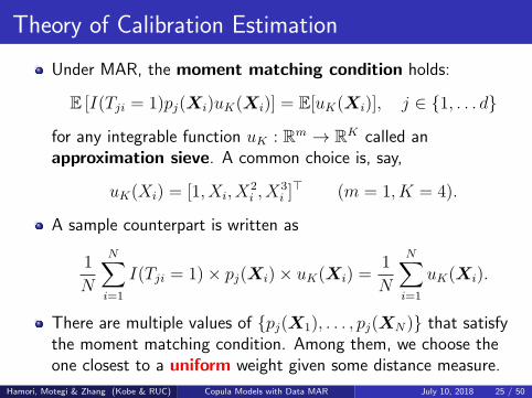
Under MAR, the moment matching condition holds:
E [I(Tji = 1)pj(Xi)uK(Xi)] = E[uK(Xi)], j ∈ {1, . . . d}
for any integrable function uK : Rm → RK called anapproximation sieve. A common choice is, say,
uK(Xi) = [1, Xi, X2i , X
3i ]
⊤ (m = 1, K = 4).
A sample counterpart is written as
1
N
N∑i=1
I(Tji = 1)× pj(Xi)× uK(Xi) =1
N
N∑i=1
uK(Xi).
There are multiple values of {pj(X1), . . . , pj(XN)} that satisfythe moment matching condition. Among them, we choose theone closest to a uniform weight given some distance measure.
Hamori, Motegi & Zhang (Kobe & RUC) Copula Models with Data MAR July 10, 2018 25 / 50
Theory of Calibration Estimation
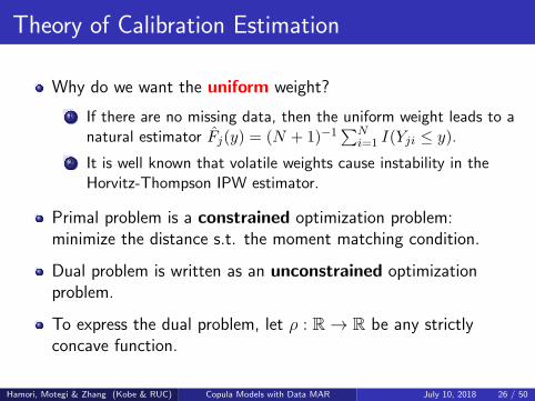
Why do we want the uniform weight?
1 If there are no missing data, then the uniform weight leads to anatural estimator Fj(y) = (N + 1)−1
∑Ni=1 I(Yji ≤ y).
2 It is well known that volatile weights cause instability in theHorvitz-Thompson IPW estimator.
Primal problem is a constrained optimization problem:minimize the distance s.t. the moment matching condition.
Dual problem is written as an unconstrained optimizationproblem.
To express the dual problem, let ρ : R → R be any strictlyconcave function.
Hamori, Motegi & Zhang (Kobe & RUC) Copula Models with Data MAR July 10, 2018 26 / 50
Theory of Calibration Estimation
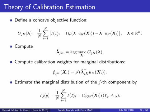
Define a concave objective function:
GjK(λ) =1
N
N∑i=1
[I(Tji = 1)ρ(λ⊤uK(Xi))− λ⊤uK(Xi)
], λ ∈ RK .
ComputeλjK = argmax
λGjK(λ).
Compute calibration weights for marginal distributions:
pjK(Xi) = ρ′(λ⊤jKuK(Xi)).
Estimate the marginal distribution of the j-th component by
Fj(y) =1
N
N∑i=1
I(Tji = 1)pjK(Xi)I(Yji ≤ y).
Hamori, Motegi & Zhang (Kobe & RUC) Copula Models with Data MAR July 10, 2018 27 / 50
Theory of Calibration Estimation
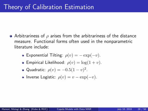
Arbitrariness of ρ arises from the arbitrariness of the distancemeasure. Functional forms often used in the nonparametricliterature include:
Exponential Tilting: ρ(v) = − exp(−v).
Empirical Likelihood: ρ(v) = log(1 + v).
Quadratic: ρ(v) = −0.5(1− v)2.
Inverse Logistic: ρ(v) = v − exp(−v).
Hamori, Motegi & Zhang (Kobe & RUC) Copula Models with Data MAR July 10, 2018 28 / 50
Theory of Calibration Estimation
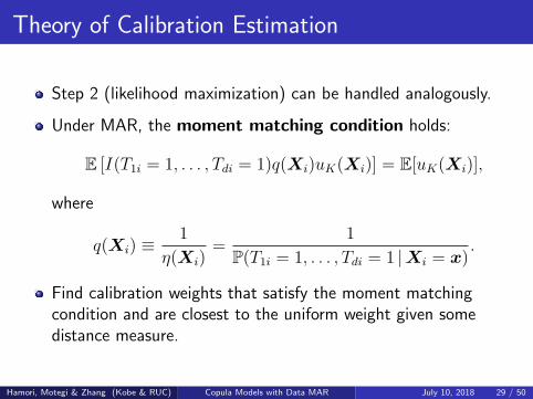
Step 2 (likelihood maximization) can be handled analogously.
Under MAR, the moment matching condition holds:
E [I(T1i = 1, . . . , Tdi = 1)q(Xi)uK(Xi)] = E[uK(Xi)],
where
q(Xi) ≡1
η(Xi)=
1
P(T1i = 1, . . . , Tdi = 1 |Xi = x).
Find calibration weights that satisfy the moment matchingcondition and are closest to the uniform weight given somedistance measure.
Hamori, Motegi & Zhang (Kobe & RUC) Copula Models with Data MAR July 10, 2018 29 / 50
Theory of Calibration Estimation
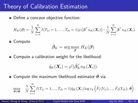
Define a concave objective function:
HK(β) =1
N
N∑i=1
I(T1i = 1, . . . , Tdi = 1)ρ(β⊤uK(Xi)
)− 1
N
N∑i=1
β⊤uK(Xi).
ComputeβK = argmax
βHK(β).
Compute a calibration weight for the likelihood:
qK(Xi) = ρ′(β⊤KuK(Xi)).
Compute the maximum likelihood estimator θ via
maxθ∈Θ
1
N
N∑i=1
I(T1i = 1, ..., Tdi = 1)qK(Xi) log cd
(F1(Y1i), ..., Fd(Ydi); θ
).
Hamori, Motegi & Zhang (Kobe & RUC) Copula Models with Data MAR July 10, 2018 30 / 50
Theory of Calibration Estimation
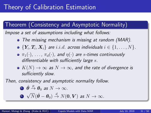
Theorem (Consistency and Asymptotic Normality)
Impose a set of assumptions including what follows:
The missing mechanism is missing at random (MAR).
{Yi,Ti,Xi} are i.i.d. across individuals i ∈ {1, . . . , N}.π1(·), . . . , πd(·), and η(·) are s-times continuouslydifferentiable with sufficiently large s.
K(N) → ∞ as N → ∞, and the rate of divergence issufficiently slow.
Then, consistency and asymptotic normality follow.
1 θp→ θ0 as N → ∞.
2
√N(θ − θ0)
d→ N(0,V ) as N → ∞.
Hamori, Motegi & Zhang (Kobe & RUC) Copula Models with Data MAR July 10, 2018 31 / 50

Theory of Calibration Estimation
The asymptotic covariance matrix V is expressed as
V = B−1ΣB−1.
We can construct consistent estimators for B and Σ, and hence
V = B−1ΣB−1 p→ V .
See the main paper for a complete set of assumptions, proofs ofthe consistency and asymptotic normality, and the constructionof V and V .
Hamori, Motegi & Zhang (Kobe & RUC) Copula Models with Data MAR July 10, 2018 32 / 50

Monte Carlo Simulations: DGP
Target variables are Yi = [Y1i, Y2i]⊤ (d = 2).
Consider a scalar covariate Xi.
Define Ui = [U1i, U2i, U3i]⊤ = [F1(Y1i), F2(Y2i), FX(Xi)]
⊤.
F1(·) is the marginal distribution of Y1i, and we use N(0, 1).
F2(·) is the marginal distribution of Y2i, and we use N(0, 1).
FX(·) is the marginal distribution of Xi, and we use N(0, 1).
The inverse distribution functions F−11 (·), F−1
2 (·), and F−1X (·)
are known and tractable.
Hamori, Motegi & Zhang (Kobe & RUC) Copula Models with Data MAR July 10, 2018 33 / 50
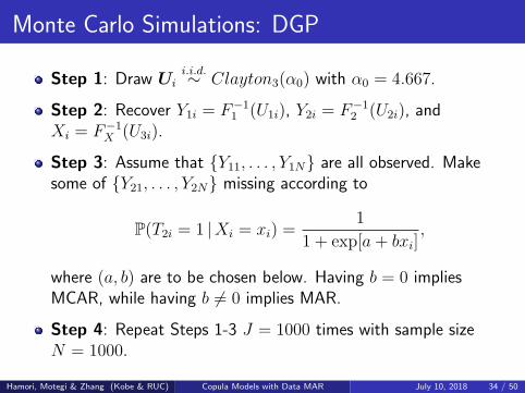
Monte Carlo Simulations: DGP
Step 1: Draw Uii.i.d.∼ Clayton3(α0) with α0 = 4.667.
Step 2: Recover Y1i = F−11 (U1i), Y2i = F−1
2 (U2i), andXi = F−1
X (U3i).
Step 3: Assume that {Y11, . . . , Y1N} are all observed. Makesome of {Y21, . . . , Y2N} missing according to
P(T2i = 1 |Xi = xi) =1
1 + exp[a+ bxi],
where (a, b) are to be chosen below. Having b = 0 impliesMCAR, while having b = 0 implies MAR.
Step 4: Repeat Steps 1-3 J = 1000 times with sample sizeN = 1000.
Hamori, Motegi & Zhang (Kobe & RUC) Copula Models with Data MAR July 10, 2018 34 / 50
Monte Carlo Simulations: DGP
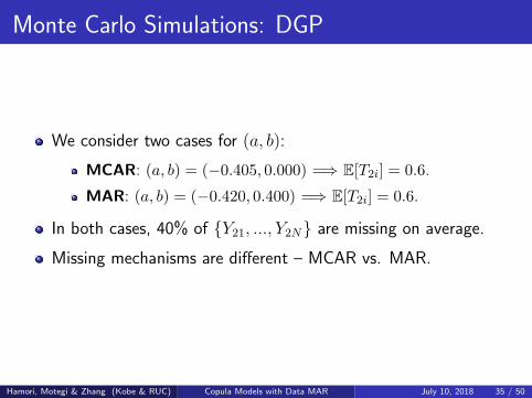
We consider two cases for (a, b):
MCAR: (a, b) = (−0.405, 0.000) =⇒ E[T2i] = 0.6.
MAR: (a, b) = (−0.420, 0.400) =⇒ E[T2i] = 0.6.
In both cases, 40% of {Y21, ..., Y2N} are missing on average.
Missing mechanisms are different – MCAR vs. MAR.
Hamori, Motegi & Zhang (Kobe & RUC) Copula Models with Data MAR July 10, 2018 35 / 50
Monte Carlo Simulations: Estimation
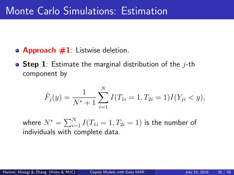
Approach #1: Listwise deletion.
Step 1: Estimate the marginal distribution of the j-thcomponent by
Fj(y) =1
N∗ + 1
N∑i=1
I(T1i = 1, T2i = 1)I(Yji < y),
where N∗ =∑N
i=1 I(T1i = 1, T2i = 1) is the number ofindividuals with complete data.
Hamori, Motegi & Zhang (Kobe & RUC) Copula Models with Data MAR July 10, 2018 36 / 50
Monte Carlo Simulations: Estimation
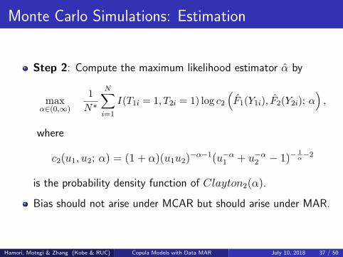
Step 2: Compute the maximum likelihood estimator α by
maxα∈(0,∞)
1
N∗
N∑i=1
I(T1i = 1, T2i = 1) log c2
(F1(Y1i), F2(Y2i); α
),
where
c2(u1, u2; α) = (1 + α)(u1u2)−α−1(u−α
1 + u−α2 − 1)−
1α−2
is the probability density function of Clayton2(α).
Bias should not arise under MCAR but should arise under MAR.
Hamori, Motegi & Zhang (Kobe & RUC) Copula Models with Data MAR July 10, 2018 37 / 50
Monte Carlo Simulations: Estimation
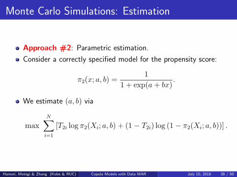
Approach #2: Parametric estimation.
Consider a correctly specified model for the propensity score:
π2(x; a, b) =1
1 + exp(a+ bx).
We estimate (a, b) via
maxN∑i=1
[T2i log π2(Xi; a, b) + (1− T2i) log (1− π2(Xi; a, b))] .
Hamori, Motegi & Zhang (Kobe & RUC) Copula Models with Data MAR July 10, 2018 38 / 50

Monte Carlo Simulations: Estimation
Compute
p2(Xi) = q(Xi) =1
π2(Xi; a, b).
Estimate marginal distributions by
Fj(y) =1
N
N∑i=1
I(Tji = 1)pj(Xi)I(Yji < y).
Estimate the copula parameter α via
maxα∈(0,∞)
1
N
N∑i=1
I(T1i = 1, T2i = 1)q(Xi) log c2
(F1(Y1i), F2(Y2i); α
).
Hamori, Motegi & Zhang (Kobe & RUC) Copula Models with Data MAR July 10, 2018 39 / 50
Monte Carlo Simulations: Estimation
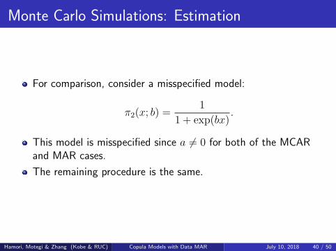
For comparison, consider a misspecified model:
π2(x; b) =1
1 + exp(bx).
This model is misspecified since a = 0 for both of the MCARand MAR cases.
The remaining procedure is the same.
Hamori, Motegi & Zhang (Kobe & RUC) Copula Models with Data MAR July 10, 2018 40 / 50
Monte Carlo Simulations: Estimation
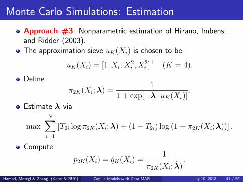
Approach #3: Nonparametric estimation of Hirano, Imbens,and Ridder (2003).
The approximation sieve uK(Xi) is chosen to be
uK(Xi) = [1, Xi, X2i , X
3i ]
⊤ (K = 4).
Define
π2K(Xi;λ) =1
1 + exp[−λ⊤uK(Xi)].
Estimate λ via
maxN∑i=1
[T2i log π2K(Xi;λ) + (1− T2i) log (1− π2K(Xi;λ))] .
Compute
p2K(Xi) = qK(Xi) =1
π2K(Xi; λ).
Hamori, Motegi & Zhang (Kobe & RUC) Copula Models with Data MAR July 10, 2018 41 / 50

Monte Carlo Simulations: Estimation
The nonparametric approach with K = 2 is essentially identicalto the parametric approach with the correctly specified model.
This is just a coincidence given that the true missing mechanismobeys a logistic function.
In theory, K → ∞ as N → ∞ and the nonparametric approachleads to a consistent estimator for any missing mechanism.
Finite sample performance is another question.
Hamori, Motegi & Zhang (Kobe & RUC) Copula Models with Data MAR July 10, 2018 42 / 50
Monte Carlo Simulations: Estimation
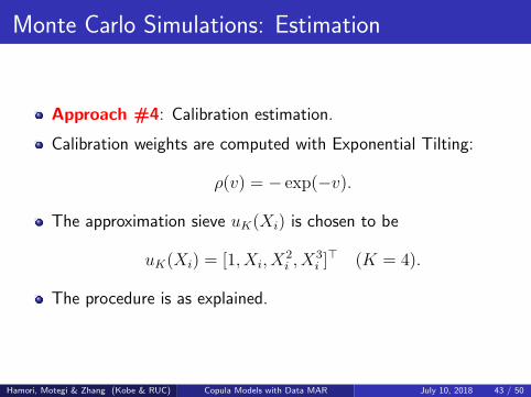
Approach #4: Calibration estimation.
Calibration weights are computed with Exponential Tilting:
ρ(v) = − exp(−v).
The approximation sieve uK(Xi) is chosen to be
uK(Xi) = [1, Xi, X2i , X
3i ]
⊤ (K = 4).
The procedure is as explained.
Hamori, Motegi & Zhang (Kobe & RUC) Copula Models with Data MAR July 10, 2018 43 / 50
Monte Carlo Simulations: Results
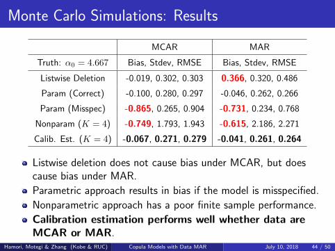
MCAR MAR
Truth: α0 = 4.667 Bias, Stdev, RMSE Bias, Stdev, RMSE
Listwise Deletion -0.019, 0.302, 0.303 0.366, 0.320, 0.486
Param (Correct) -0.100, 0.280, 0.297 -0.046, 0.262, 0.266
Param (Misspec) -0.865, 0.265, 0.904 -0.731, 0.234, 0.768
Nonparam (K = 4) -0.749, 1.793, 1.943 -0.615, 2.186, 2.271
Calib. Est. (K = 4) -0.067, 0.271, 0.279 -0.041, 0.261, 0.264
Listwise deletion does not cause bias under MCAR, but doescause bias under MAR.
Parametric approach results in bias if the model is misspecified.
Nonparametric approach has a poor finite sample performance.
Calibration estimation performs well whether data areMCAR or MAR.
Hamori, Motegi & Zhang (Kobe & RUC) Copula Models with Data MAR July 10, 2018 44 / 50

Monte Carlo Simulations: Results
-3 -2 -1 0 1 2 3 4
Y1
-3
-2
-1
0
1
2
3
4
Y2
Missing
Observed
0 = 4.667
LD = 5.085 (Bias = 0.418)
CE = 4.625 (Bias = -0.042)
A MC Sample (N = 500)
14
1.5
42
q(X
)
2
Y2
20
Y1
2.5
0-2 -2
Calibration Weights
Clayton has lower-tail dependence and upper-tail independence.
Missing data arise more often at the upper tail and hence theassociation appears to be stronger than what it is.
Hence listwise deletion results in positive bias.
CE avoids bias by putting larger weights at the upper tail.
Hamori, Motegi & Zhang (Kobe & RUC) Copula Models with Data MAR July 10, 2018 45 / 50
Conclusions
We investigate the estimation of semiparametric copulamodels under missing data for the first time in the literature.
There is analogy between missing data and average treatmenteffects since observing or not observing data is a binaryphenomenon.
Chan, Yam, and Zhang (2016) propose the calibrationestimation for average treatment effects.
We apply the calibration estimation to missing data for the firsttime in the literature.
Hamori, Motegi & Zhang (Kobe & RUC) Copula Models with Data MAR July 10, 2018 46 / 50

Conclusions
The calibration estimator satisfies consistency and asymptoticnormality under some assumptions including i.i.d. data and themissing at random (MAR) mechanism.
We also derive a consistent estimator for the asymptoticcovariance matrix.
In view of the simulation results, the calibration estimatordominates listwise deletion, parametric approach, andnonparametric approach.
Hamori, Motegi & Zhang (Kobe & RUC) Copula Models with Data MAR July 10, 2018 47 / 50
References
Bang, H. and J. M. Robins (2005). Doubly Robust Estimation inMissing Data and Causal Inference Models. Biometrics, 61, 962-973.
Chan, K. C. G., S. C. P. Yam, and Z. Zhang (2016). GloballyEfficient Non-Parametric Inference of Average Treatment Effects byEmpirical Balancing Calibration Weighting. Journal of the RoyalStatistical Society, Series B, 78, 673-700.
Chen, X., H. Hong, and A. Tarozzi (2008). SemiparametricEfficiency in GMM Models with Auxiliary Data. The Annals ofStatistics, 36, 808-843.
Hahn, J. (1998). On the Role of the Propensity Score in EfficientSemiparametric Estimation of Average Treatment Effects.Econometrica, 66, 315-331.
Hamori, Motegi & Zhang (Kobe & RUC) Copula Models with Data MAR July 10, 2018 48 / 50
References
Hirano, K., G. W. Imbens, and G. Ridder (2003). EfficientEstimation of Average Treatment Effects Using the EstimatedPropensity Score. Econometrica, 71, 1161-1189.
Horvitz, D. G. and D. J. Thompson (1952). A Generalization ofSampling without Replacement from a Finite Universe. Journal ofthe American Statistical Association, 47, 663-685.
Imbens, G. W., W. K. Newey, and G. Ridder (2005).Mean-square-error Calculations for Average Treatment Effects. IEPRWorking Paper No. 05.34.
Lawless, J. F., J. D. Kalbfleisch, and C. J. Wild (1999).Semiparametric Methods for Response-Selective and Missing DataProblems in Regression. Journal of the Royal Statistical Society,Series B, 61, 413-438.
Hamori, Motegi & Zhang (Kobe & RUC) Copula Models with Data MAR July 10, 2018 49 / 50
References
Robins, J. M., A. Rotnitzky, and L. P. Zhao (1994). Estimation ofRegression Coefficients When Some Regressors are not AlwaysObserved. Journal of the American Statistical Association, 89,846-866.
Rubin, D. B. (1976). Inference and Missing Data. Biometrika, 63,581-592.
Sklar, A. (1959). Fonctions de repartition a n dimensions et leursmarges. Publications de l’Institut de Statistique de L’Universite deParis, 8, 229-231.
Zhao, L. P. and S. Lipsitz (1992). Designs and Analysis ofTwo-Stage Studies. Statistics in Medicine, 11, 769-782.
Hamori, Motegi & Zhang (Kobe & RUC) Copula Models with Data MAR July 10, 2018 50 / 50