
Calibrated Submanifolds and the Exceptional Geometries
172
Calibrated Submanifolds and the Exceptional Geometries Jason Dean Lotay Christ Church University of Oxford A thesis submitted for the degree of Doctor of Philosophy Trinity Term 2005
Transcript of Calibrated Submanifolds and the Exceptional Geometries
Calibrated Submanifolds
and the
Exceptional Geometries
Jason Dean Lotay
Christ Church
University of Oxford
A thesis submitted for the degree of
Doctor of Philosophy
Trinity Term 2005

To Mom and Dad, without whom none of this would have been possible.

Acknowledgements
First and foremost I wish to thank my supervisor Dominic Joyce for his tireless efforts
in guiding me through the research that has culminated in this thesis. It has been a
pleasure being his student and I am indebted to him for all his help in the past three
years.
I would also like to thank all my family and friends, paying particular tribute to my
parents for their love and support, my brother Gavin for, amongst many other things,
helping me (slightly unwittingly!) to solve a problem, and to my girlfriend Vicky for her
love, patience and understanding.
Finally, I must thank my examiners, Andrew Dancer and Alexei Kovalev, for their helpful
advice and EPSRC for providing the funding for this research project.
Contents
Preface v
1 Introduction 1
1.1 Calibrated Geometry . . . . . . . . . . . . . . . . . . . . . . . . . . . . . . . . . . . . 2
1.2 Asymptotics . . . . . . . . . . . . . . . . . . . . . . . . . . . . . . . . . . . . . . . . . 3
1.3 Number Systems . . . . . . . . . . . . . . . . . . . . . . . . . . . . . . . . . . . . . . 5
2 The Exceptional Geometries 6
2.1 The Octonions . . . . . . . . . . . . . . . . . . . . . . . . . . . . . . . . . . . . . . . 6
2.1.1 Cayley multiplication table . . . . . . . . . . . . . . . . . . . . . . . . . . . . 6
2.1.2 Cross products . . . . . . . . . . . . . . . . . . . . . . . . . . . . . . . . . . . 7
2.1.3 G2 and Spin(7) . . . . . . . . . . . . . . . . . . . . . . . . . . . . . . . . . . . 9
2.2 Holonomy Groups . . . . . . . . . . . . . . . . . . . . . . . . . . . . . . . . . . . . . 10
2.3 The G2 Calibrations . . . . . . . . . . . . . . . . . . . . . . . . . . . . . . . . . . . . 12
2.3.1 G2 geometry on R7 . . . . . . . . . . . . . . . . . . . . . . . . . . . . . . . . . 12
2.3.2 G2 structures on 7-manifolds . . . . . . . . . . . . . . . . . . . . . . . . . . . 14
2.4 The Spin(7) Calibration . . . . . . . . . . . . . . . . . . . . . . . . . . . . . . . . . . 15
2.4.1 Spin(7) geometry on R8 . . . . . . . . . . . . . . . . . . . . . . . . . . . . . . 15
2.4.2 Spin(7) structures on 8-manifolds . . . . . . . . . . . . . . . . . . . . . . . . . 18
I Constructions in Euclidean Space 20
3 Special Lagrangian m-folds in Cm 21
3.1 Basic Theory . . . . . . . . . . . . . . . . . . . . . . . . . . . . . . . . . . . . . . . . 21
3.2 Evolution Equations . . . . . . . . . . . . . . . . . . . . . . . . . . . . . . . . . . . . 23
3.3 An Explicit Construction in C3 . . . . . . . . . . . . . . . . . . . . . . . . . . . . . . 25
i

4 Associative 3-folds in R7 28
4.1 The First Evolution Equation . . . . . . . . . . . . . . . . . . . . . . . . . . . . . . . 28
4.2 Constructions Using Symmetries . . . . . . . . . . . . . . . . . . . . . . . . . . . . . 29
4.2.1 A subgroup of R×U(1)2 . . . . . . . . . . . . . . . . . . . . . . . . . . . . . 29
4.2.2 U(1)-invariant cones . . . . . . . . . . . . . . . . . . . . . . . . . . . . . . . . 33
4.3 The Second Evolution Equation . . . . . . . . . . . . . . . . . . . . . . . . . . . . . . 38
4.4 An Explicit Affine Evolution Construction . . . . . . . . . . . . . . . . . . . . . . . . 39
4.4.1 Singularities . . . . . . . . . . . . . . . . . . . . . . . . . . . . . . . . . . . . . 41
4.4.2 Solving the equations . . . . . . . . . . . . . . . . . . . . . . . . . . . . . . . 43
4.4.3 Periodicity . . . . . . . . . . . . . . . . . . . . . . . . . . . . . . . . . . . . . 48
4.5 1-Ruled Associative 3-folds . . . . . . . . . . . . . . . . . . . . . . . . . . . . . . . . 50
4.5.1 The associative condition . . . . . . . . . . . . . . . . . . . . . . . . . . . . . 51
4.5.2 The partial differential equations . . . . . . . . . . . . . . . . . . . . . . . . . 55
4.5.3 Holomorphic vector fields . . . . . . . . . . . . . . . . . . . . . . . . . . . . . 57
4.5.4 Examples . . . . . . . . . . . . . . . . . . . . . . . . . . . . . . . . . . . . . . 59
5 Coassociative 4-folds in R7 and Cayley 4-folds in R8 60
5.1 Evolution Equations . . . . . . . . . . . . . . . . . . . . . . . . . . . . . . . . . . . . 60
5.2 Coassociative 4-folds with Symmetries . . . . . . . . . . . . . . . . . . . . . . . . . . 62
5.2.1 U(1)2-invariant cones . . . . . . . . . . . . . . . . . . . . . . . . . . . . . . . 62
5.2.2 SU(2) symmetry 1 . . . . . . . . . . . . . . . . . . . . . . . . . . . . . . . . . 63
5.2.3 SU(2) symmetry 2 . . . . . . . . . . . . . . . . . . . . . . . . . . . . . . . . . 66
5.3 Cayley 4-folds with Symmetries . . . . . . . . . . . . . . . . . . . . . . . . . . . . . . 68
5.3.1 U(1)2-invariant cones . . . . . . . . . . . . . . . . . . . . . . . . . . . . . . . 68
5.3.2 SU(2) symmetry 1 . . . . . . . . . . . . . . . . . . . . . . . . . . . . . . . . . 69
5.3.3 SU(2) symmetry 2 . . . . . . . . . . . . . . . . . . . . . . . . . . . . . . . . . 72
5.3.4 Some U(1)-invariant examples . . . . . . . . . . . . . . . . . . . . . . . . . . . 73
5.4 2-Ruled Calibrated 4-folds in R7 and R8 . . . . . . . . . . . . . . . . . . . . . . . . . 75
5.4.1 The partial differential equations . . . . . . . . . . . . . . . . . . . . . . . . . 76
5.4.2 Gauge transformations . . . . . . . . . . . . . . . . . . . . . . . . . . . . . . . 82
5.4.3 Planar 2-ruled Cayley 4-folds . . . . . . . . . . . . . . . . . . . . . . . . . . . 84
5.4.4 Main results . . . . . . . . . . . . . . . . . . . . . . . . . . . . . . . . . . . . . 85
5.4.5 Holomorphic vector fields . . . . . . . . . . . . . . . . . . . . . . . . . . . . . 89
5.4.6 Examples . . . . . . . . . . . . . . . . . . . . . . . . . . . . . . . . . . . . . . 91
ii
II Noncompact Coassociative Deformations 95
6 Analysis on Noncompact Riemannian Manifolds 96
6.1 AC and CS Manifolds . . . . . . . . . . . . . . . . . . . . . . . . . . . . . . . . . . . 96
6.2 Weighted Banach Spaces . . . . . . . . . . . . . . . . . . . . . . . . . . . . . . . . . . 98
6.3 Uniformly Elliptic AC and CS Operators . . . . . . . . . . . . . . . . . . . . . . . . . 101
6.3.1 Fredholm theory . . . . . . . . . . . . . . . . . . . . . . . . . . . . . . . . . . 101
6.3.2 Index theory . . . . . . . . . . . . . . . . . . . . . . . . . . . . . . . . . . . . 104
6.4 Elliptic Regularity . . . . . . . . . . . . . . . . . . . . . . . . . . . . . . . . . . . . . 106
6.5 Hodge Theory . . . . . . . . . . . . . . . . . . . . . . . . . . . . . . . . . . . . . . . . 107
7 Deformation Theory of Asymptotically Conical Coassociative 4-folds 109
7.1 The Deformation Map . . . . . . . . . . . . . . . . . . . . . . . . . . . . . . . . . . . 110
7.1.1 Preliminaries . . . . . . . . . . . . . . . . . . . . . . . . . . . . . . . . . . . . 110
7.1.2 The map F and the associated map G . . . . . . . . . . . . . . . . . . . . . . 111
7.1.3 Regularity . . . . . . . . . . . . . . . . . . . . . . . . . . . . . . . . . . . . . . 115
7.2 Study of the Cokernel . . . . . . . . . . . . . . . . . . . . . . . . . . . . . . . . . . . 116
7.2.1 The image of d + d∗ . . . . . . . . . . . . . . . . . . . . . . . . . . . . . . . . 116
7.2.2 Obstructions and the kernel of the adjoint map . . . . . . . . . . . . . . . . . 117
7.2.3 Dimension of the cokernel . . . . . . . . . . . . . . . . . . . . . . . . . . . . . 119
7.3 The Deformation Space . . . . . . . . . . . . . . . . . . . . . . . . . . . . . . . . . . 121
7.3.1 The image of F . . . . . . . . . . . . . . . . . . . . . . . . . . . . . . . . . . . 121
7.3.2 The moduli space . . . . . . . . . . . . . . . . . . . . . . . . . . . . . . . . . . 122
7.4 Dimension of the Moduli Space . . . . . . . . . . . . . . . . . . . . . . . . . . . . . . 123
7.5 Study of Rates λ < −2 . . . . . . . . . . . . . . . . . . . . . . . . . . . . . . . . . . . 127
7.6 An Example . . . . . . . . . . . . . . . . . . . . . . . . . . . . . . . . . . . . . . . . . 129
8 Deformation Theory of Coassociative 4-folds with Conical Singularities 131
8.1 Basic Theory . . . . . . . . . . . . . . . . . . . . . . . . . . . . . . . . . . . . . . . . 131
8.2 The Deformation Problems . . . . . . . . . . . . . . . . . . . . . . . . . . . . . . . . 134
8.2.1 Problem 1: fixed singularities and G2 structure . . . . . . . . . . . . . . . . . 134
8.2.2 Problem 2: moving singularities and fixed G2 structure . . . . . . . . . . . . 138
8.2.3 Problem 3: moving singularities and varying G2 structure . . . . . . . . . . . 141
8.3 The Deformation and Obstruction Spaces . . . . . . . . . . . . . . . . . . . . . . . . 145
8.3.1 Problem 1 . . . . . . . . . . . . . . . . . . . . . . . . . . . . . . . . . . . . . . 145
iii

8.3.2 Problem 2 . . . . . . . . . . . . . . . . . . . . . . . . . . . . . . . . . . . . . . 149
8.3.3 Problem 3 . . . . . . . . . . . . . . . . . . . . . . . . . . . . . . . . . . . . . . 151
8.4 Dimension Calculations . . . . . . . . . . . . . . . . . . . . . . . . . . . . . . . . . . 152
8.5 ϕ-Closed 7-Manifolds . . . . . . . . . . . . . . . . . . . . . . . . . . . . . . . . . . . . 156
Afterword: Further Research 158
Bibliography 159
iv

Preface
The knowledge of which geometry aims is the knowledge of the eternal.– Plato
Calibrated geometry, since conception, has been tied to the exceptional geometries occurring in seven
and eight dimensions. Harvey and Lawson [17, §IV], in their seminal paper on the subject, dedicate
a chapter to the relationship between these two fields. In seven dimensions the relevant holonomy
group is G2 and the calibrated submanifolds are known as associative 3-folds and coassociative
4-folds, whereas in eight the group is Spin(7) and Cayley 4-folds form the calibrated geometry.
The dearth of concrete formulations of calibrated submanifolds in manifolds with exceptional
holonomy, even in the simple cases of 7- and 8-dimensional Euclidean space, is markedly evident.
The exhibition of examples in mathematics, perhaps particularly in geometry, is crucial to our un-
derstanding of the theory involved. Part I of this thesis addresses this need by presenting methods
of constructing calibrated submanifolds of R7 and R8 related to the exceptional geometries and,
moreover, utilising them to produce explicit descriptions of associative, coassociative and Cayley
submanifolds. Much of this work has already appeared in the author’s papers [38] and [39]: specifi-
cally, Chapter 4, apart from §4.2, and §5.4 form the material of the former and the latter respectively,
with the addition of further examples.
Having studied what one may tentatively label the ‘applied’ aspects of the subject, Part 2 tackles,
remaining cautious with our verbiage, more ‘abstract’ problems. It is concerned with deformations
of two distinguished classes of noncompact coassociative 4-folds which are, in a sense, dual to one
another: asymptotically conical (AC) and 4-folds with conical singularities (CS). Informally, AC
submanifolds ‘look like’ cones near infinity, whereas CS submanifolds have a finite number of points
at which they locally have the appearance of a cone near its vertex. McLean [45, §4] fully describes
the deformation theory of compact coassociative 4-folds, demonstrating that the moduli space of
deformations is a smooth manifold of known dimension. This result motivates our study as both
AC and CS submanifolds are natural extensions from the compact case. The material in Chapter 7
on AC deformations forms the core of the author’s paper [40].
v

The incentive for the research detailed within this dissertation is not limited to mathematics. In
high-energy theoretical physics there are areas of study known as String Theory, M-theory and F-
theory. The ultimate goal of String Theory is to combine Quantum Theory and General Relativity.
The key concept is that particles are not modelled as points in space but rather as a 1-dimensional
object, called a ‘string’. An unusual feature of the theory is that the universe is forced to have a
dimension higher than four. The most popular version of String Theory requires the universe to
have ten dimensions. However, the dimension of the universe may be eleven (for M-theory), twelve
(for F-theory) or possibly even twenty-six.
String theorists hypothesise that, geometrically, the universe comprises a large, observable, 4-
dimensional piece and a very small extra piece which has six, seven, eight or more dimensions. For
an 11-dimensional universe the additional constituent must be a compact G2 manifold; that is, a
compact 7-dimensional Riemannian manifold with holonomy group contained in G2. Associative
and coassociative submanifolds of a G2 manifold then have physical significance in M-theory, with
a particular interest shown for their singularities. A similar picture may hold for a 12-dimensional
universe in F-theory, where the relevant 8-dimensional piece might be a Spin(7) manifold, but the
physics is as yet unclear.
An area of conjectures in String Theory is called Mirror Symmetry. There is a proposed geometric
explanation of this result for 10-dimensional String Theory known as the SYZ conjecture, which
involves the consideration of fibrations of a compact Calabi–Yau 3-fold by 3-dimensional calibrated
submanifolds, known as special Lagrangian 3-folds, that are allowed to have singularities. It has
been conjectured, based on physical arguments, that the analogous situation in seven dimensions is
true. The hope is that the work in this document will aid in the solution of this difficult problem.
It may appear that we have spent much of this preface detailing the usefulness of the research
discussed in this thesis. Although this is certainly true, it would only be honest to close with the
following quotation with which the author agrees wholeheartedly.
The mathematician does not study pure mathematics because it is useful; he studies it
because he delights in it and he delights in it because it is beautiful.
– Henri Poincare
vi

Chapter 1
Introduction
The research presented here lies within the broader subject of calibrated geometry. In this chapter the
basic theory underlying this topic is given. Certain types of asymptotic behaviour of submanifolds
at infinity are also discussed and a section is dedicated to some elementary properties of number
systems and their relationship with group theory. This final section of the chapter provides the reader
with background material before the exposition of the octonions, or Cayley numbers, in Chapter 2.
The focus of the second chapter is on the exceptional Lie groups G2 and Spin(7) and the formula-
tion of calibrations on R7 and R8 which are associated to these groups. This allows the definition of
associative 3-folds and coassociative 4-folds in R7 and Cayley 4-folds in R8. Moreover, it is demon-
strated that there is a generalisation of these calibrations and calibrated submanifolds for particular
7- and 8-dimensional Riemannian manifolds, known as G2 and Spin(7) manifolds respectively.
Following these two preliminary chapters, the rest of the dissertation is split into two parts
each containing three chapters. Part I begins, in Chapter 3, with a review of the theory and
constructions of special Lagrangian m-folds in Cm which shall be pertinent in the sequel. Chapter
4 gives construction methods and examples for associative 3-folds in R7. The final chapter in Part
I is a similar presentation for coassociative 4-folds in R7 and Cayley 4-folds in R8.
Chapter 6, the first chapter in Part II, reviews various definitions and results from the study
of analysis on asymptotically conical (AC) manifolds and manifolds with conical singularities (CS).
This material is predominately based on a paper by Lockhart and McOwen [37]. The final chapters
are dedicated to the study of deformations of AC coassociative 4-folds in R7 and CS coassocia-
tive 4-folds in a G2 manifold. In Chapter 7 it is proved that an AC coassociative 4-fold, which
converges with generic rate in a specified range to a cone at infinity, has a locally smooth moduli
space of deformations of known dimension. In Chapter 8, three different deformation problems for
CS coassociative 4-folds are studied. For each case there is a weaker result: the moduli space is
1

locally homeomorphic to the kernel of a smooth map between smooth manifolds. However, if the
obstructions in the problem are known to be zero, the moduli space is locally smooth and a lower
bound is given on its dimension.
In this thesis, manifolds are taken to be smooth and nonsingular almost everywhere and sub-
manifolds are assumed to be immersed, unless otherwise stated.
1.1 Calibrated Geometry
We define calibrations and calibrated submanifolds following the approach in [17].
Definition 1.1.1. Let (M, g) be a Riemannian manifold. An oriented tangent k-plane V on M is
an oriented k-dimensional vector subspace V of TxM , for some x in M . Given an oriented tangent
k-plane V on M , g|V is a Euclidean metric on V and hence, using g|V and the orientation on V ,
there is a natural volume form, volV , which is a k-form on V .
A closed k-form η on M is a calibration on M if η|V ≤ volV for all oriented tangent k-planes V
on M , where η|V = κ · volV for some κ ∈ R, so η|V ≤ volV if κ ≤ 1. An oriented k-dimensional
submanifold N of M is a calibrated submanifold or η-submanifold if η|TxN = volTxN for all x ∈ N .
Calibrated submanifolds are minimal submanifolds [17, Theorem II.4.2]. Minimal submanifolds
of Rn are related to harmonic functions, i.e. functions f satisfying ∆f = d∗df = 0, by the following
elementary result [35, Corollary 9].
Theorem 1.1.2. A submanifold of Rn, with immersion ι, is minimal if and only if ι is harmonic;
that is, each component of ι mapping to R is harmonic.
If η is a k-form satisfying the restrictions in Definition 1.1.1 but is not closed, η-submanifolds are
no longer minimal, yet may still be defined. We shall return to this point in Sections 2.3.2 and 2.4.2
and, with greatest interest, in §8.5. However, the minimality of calibrated submanifolds provides
the following property, as discussed in [17].
Theorem 1.1.3. A calibrated submanifold is real analytic wherever it is nonsingular.
One may think of the calibrated condition as corresponding to a partial differential equation
which has solutions described by calibrated submanifolds. Given the analytic techniques employed
in this thesis and the many appearances which differential equations make during the course of our
study, this viewpoint is one we encourage the reader to adopt. Having chosen this perspective,
the inherent difficulty we face lies within the fact that the calibrations we consider correspond to
equations that are strictly nonlinear, for which solutions are hard to find in general.
2
A particular result from the theory of partial differential equations that we use is the Cauchy–
Kowalevsky Theorem [48, Theorem B.1], which we now state.
Theorem 1.1.4 (Cauchy–Kowalevsky Theorem). Let u = (u1, . . . , uN ) = u(x, t) be a vector-
valued function of x = (x1, . . . , xn) ∈ Rn and t ∈ R. Let aijk and bj be real analytic functions of
z = (x,u) in a neighbourhood of zero in Rn+N for i = 1, . . . , n and j, k = 1, . . . , N . The system of
differential equations
∂uj
∂t= bj (z) +
n∑
i=1
N∑
k=1
aijk(z)
∂uk
∂xi, j = 1, . . . , N,
with initial condition u(x, 0) = 0 has a real analytic solution in a neighbourhood of zero in Rn+1.
Moreover, this solution is unique in the class of real analytic functions.
1.2 Asymptotics
On a number of occasions we study the asymptotic behaviour of submanifolds and thus make a few
definitions relating to this area.
Definition 1.2.1. Let M and M0 be closed submanifolds of Rn. We say that M is asymptotic with
rate λ at infinity in Rn to M0 if there exist constants R > 0 and λ < 1, a compact subset K of M
and a diffeomorphism Ψ : M0 \ BR → M \K such that
|Ψ(x)− x| = O(rλ) as r →∞,
where r is the radius function on Rn and BR is the closed ball of radius R.
We continue by considering cones and conical behaviour at infinity, using the convention that
N = 0, 1, 2, . . ..
Definition 1.2.2. A cone in Rn is a submanifold of Rn which is invariant under dilations and is
nonsingular except possibly at 0. A cone C is said to be two-sided if C = −C.
Definition 1.2.3. Let M0 be a closed cone in Rn and let M be a closed nonsingular submanifold
of Rn. Then M is asymptotically conical (AC) to M0 with rate λ if there exist constants R > 0 and
λ < 1, a compact subset K of M and a diffeomorphism Ψ : M0 \ BR → M \K such that
|∇j(Ψ(x)− ι(x))| = O(rλ−j) for j ∈ N as r →∞, (1.1)
where BR is the closed ball of radius R in Rn, ι : M0 → Rn is the inclusion map and r is the radius
function on Rn. Here | . | is calculated using the cone metric on M0 \ BR, and ∇ is a combination
of the Levi–Civita connection derived from the cone metric and the flat connection on Rn acting as
partial differentiation.
3

If λ ≥ 0 in the definition above, M is AC with rate λ to any translation of M0 in Rn, since
translations correspond to O(1) displacements. If we could take λ ≥ 1, M would be AC with rate λ
to any SO(n)nRn transformation of M0, since rotations in Rn are O(r) displacements, which would
be a very weak kind of convergence.
The proposition below shows the relationship of AC behaviour to calibrated geometry.
Proposition 1.2.4. Let η be a calibration k-form on Rn and let M be an η-submanifold of Rn
which is AC with rate λ to a closed cone M0 in Rn. Provided M0 is k-dimensional, it is calibrated
with respect to η.
Proof. Use the notation of Definition 1.2.3. Write M0 = (0,∞)×Σ, where Σ = M0∩Sn−1, let (r, σ)
be coordinates on M0 and let gΣ be the induced metric on Σ from the round metric on Sn−1. Note
that there are two different metrics on M0: the cylindrical metric gcyl = dr2 + gΣ and the conical
metric gcone = dr2 + r2gΣ.
Let g0 be the Euclidean metric on Rn. Since M is calibrated with respect to η,∣∣∣dΨ|∗(r, σ)(η)
∣∣∣dΨ|∗(r, σ)(g0)
= 1 and hence∣∣∣r−kdΨ|∗(r, σ)(η)
∣∣∣r−2dΨ|∗(r, σ)(g0)
= 1 (1.2)
by the scaling properties of η and g0 under dilations.
From (1.1), ∣∣∣dΨ|∗(r, σ)(η)− dι|∗(r, σ)(η)∣∣∣gcone
= O(rλ−1) as r →∞.
Therefore, ∣∣∣r−kdΨ|∗(r, σ)(η)− r−kdι|∗(r, σ)(η)∣∣∣gcyl
= O(rλ−1) as r →∞ (1.3)
by the relationship between gcone and gcyl. Similarly,∣∣∣r−2dΨ|∗(r, σ)(g0)− r−2dι|∗(r, σ)(g0)
∣∣∣gcyl
= O(rλ−1) as r →∞. (1.4)
Since λ < 1, rλ−1 → 0 as r →∞. Moreover, gcyl is independent of r, so using (1.2)-(1.4) we deduce∣∣∣r−kdι|∗(r, σ)(η)
∣∣∣r−2dι|∗(r, σ)(g0)
→ 1 as r →∞.
However, since ι(r, σ) = rσ, r−kdι|∗(r, σ)(η) and r−2dι|∗(r, σ)(g0) are independent of r. Thus, dι∗(η) is
equal to the volume form with respect to dι∗(g0) on T(1, σ)M0 for all σ ∈ Σ. Finally note that, since
M0 is a cone, T(r, σ)M0 = T(1, σ)M0 for all r > 0. The result follows.
Another required result related to asymptotics is a Maximum Principle for harmonic functions
due to Hopf [35, p. 12].
Theorem 1.2.5 (Maximum Principle). Let f be a smooth function on a Riemannian manifold
M with boundary ∂M . If f is harmonic and assumes a local maximum (or minimum) at a point in
M \ ∂M it is constant.
4

1.3 Number Systems
We reiterate that throughout this document we suppose that N = 0, 1, 2, . . ..
We may define the orthogonal group O(n) as the set of n×n real matrices preserving the Euclidean
metric on Rn. Alternatively, O(n) preserves the dot product on Rn. The special orthogonal group
SO(n) is the subgroup of O(n) of determinant 1 matrices; i.e. it preserves the orientation on Rn.
Similarly, on Cn, we have the unitary and special unitary groups, U(n) and SU(n) respectively, for
which we simply replace real matrices by complex matrices. For the next stage we want to describe
the compact symplectic group Sp(n), for which we choose to consider the quaternions H.
The quaternions are a 4-dimensional generalisation of complex numbers discovered by Hamilton
in 1843. They are spanned by 1 and elements i, j and k satisfying the following multiplication law:
i j k
i −1 k −j
j −k −1 i
k j −i −1.
This can be summarised in the following elegant diagram.
Then Sp(n) is the group of n× n quaternionic matrices preserving the dot product on Hn. The ori-
entation preserving group, or ‘determinant 1’ group if you will, associated with Sp(n) is Sp(n) Sp(1).
We complete our discussion of number systems with the octonions, or Cayley numbers, O. They
are an 8-dimensional generalisation of complex numbers discovered in 1843 by Hamilton’s college
friend John Graves, but first appeared in a publication by Arthur Cayley in 1845. They will be
discussed in detail in §2.1. Here it is not as obvious to define the groups Spin(7) and G2 associated
with O to complete the sequence of groups described here, so we shall leave this until §2.1.3. However,
we hope that the reader will appreciate that, rather than G2 and Spin(7) appearing ‘out of the blue’,
they are the final stage of a natural progression often called the Cayley–Dickson process.
5

Chapter 2
The Exceptional Geometries
We study the exceptional geometries in seven and eight dimensions, described by the Lie groups
G2 and Spin(7), making extensive use of the octonions which are discussed in §2.1. In Sections 2.3
and 2.4, we expose the relationship of G2 and Spin(7) with calibrated geometry, both for Euclidean
spaces and, more generally, for certain types of Riemannian manifold.
2.1 The Octonions
The octonions, or Cayley numbers, O help us provide an elegant description of the exceptional
geometries and are used on many occasions in Chapters 4 and 5.
2.1.1 Cayley multiplication table
Let e1, . . . , e7 be a basis for ImO. Then a Cayley multiplication table for O is as shown.
1 e1 e2 e3 e4 e5 e6 e7
1 1 e1 e2 e3 e4 e5 e6 e7
e1 e1 −1 e3 −e2 e5 −e4 e7 −e6
e2 e2 −e3 −1 e1 e6 −e7 −e4 e5
e3 e3 e2 −e1 −1 −e7 −e6 e5 e4
e4 e4 −e5 −e6 e7 −1 e1 e2 −e3
e5 e5 e4 e7 e6 −e1 −1 −e3 −e2
e6 e6 −e7 e4 −e5 −e2 e3 −1 e1
e7 e7 e6 −e5 −e4 e3 e2 −e1 −1
(2.1)
This table is not standard but chosen to agree with our later conventions. The information can be
6

encoded in a diagram known as the Fano projective plane, which is referred to, for example, in [49,
p. 157].
The multiplication is neither commutative nor associative. However, there are 4-dimensional asso-
ciative subalgebras of O which, along with their complements, will be used to describe calibrated
3-planes and 4-planes in R7.
2.1.2 Cross products
We define cross products and multiple cross products of octonions which help us to describe and
interpret the geometry of R7 and R8. The material is mainly derived from [17, Appendix IV.B]. We
must note however that, because of the conventions adopted, there are some minor modifications to
the formulae given in [17]. The differences come from our choice of basis for O, so our formulae are
equivalent up to a coordinate transformation and possible reversal of orientation, amounting to a
change in sign. We endeavour to make these discrepancies apparent to the reader.
Definition 2.1.1. Let x, y, z, w ∈ O. The cross product of x and y is
x× y = −12
(xy − yx). (2.2)
Note that x× y = Im(yx), which shows that the cross product is imaginary-valued.
The triple cross product of x, y, z is
x× y × z = −12(x(yz)− z(yx)
)(2.3)
7

and the fourfold cross product of x, y, z, w is
x× y × z × w =14(x(y × z × w) + y(z × x× w) + z(x× y × w) + w(y × x× z)
). (2.4)
The triple cross product of x, y and z can also be defined as the alternation of −x(yz). Hence, the
triple and fourfold cross products are alternating multilinear forms.
Equations (2.2)-(2.3) are the opposite sign to the equivalent formulae in [17] and (2.4) is unaltered
because the sign change is already accounted for by the choice in (2.3). Note that x × y × z 6=x× (y × z) 6= (x× y)× z in general and a similar statement is true for the fourfold cross product.
We make some observations about the real parts of the products [17, Lemma IV.B.9].
Proposition 2.1.2. If x, y, z, w ∈ O and x′, y′, z′ are the imaginary parts of x, y, z respectively,
Re(x× y) = 0,
Re(x× y × z) = g0(x′ × y′, z′) and
Re(x× y × z × w) = g0(x× y × z, w),
where g0 is the Euclidean metric on O ∼= R8.
Recall the commutator [x, y] = xy − yx of x and y. This leads us to define the associator.
Definition 2.1.3. The associator [x, y, z] of x, y, z ∈ O is given by:
[x, y, z] = (xy)z − x(yz).
Whereas the commutator measures the extent to which commutativity fails, the associator gives the
degree to which associativity fails in O. In §4.4 we require some properties of the associator which
we state as a proposition taken from [17, Proposition IV.B.16].
Proposition 2.1.4. The associator [x, y, z] of x, y, z ∈ O is alternating, imaginary-valued and
orthogonal to x, y, z and to [a, b] for any subset a, b of x, y, z.
On ImO we can also define the coassociator.
Definition 2.1.5. The coassociator [x, y, z, w] of x, y, z, w ∈ ImO is given by:
[x, y, z, w] = −(g0(y, zw)x + g0(z, xw)y + g0(x, yw)z + g0(y, xz)w
),
where g0 is the Euclidean metric on ImO ∼= R7.
If we restrict to considering ImO we get the following neat result [17, Proposition IV.B.14].
8

Proposition 2.1.6. For x, y, z, w ∈ ImO,
2 Im(x× y) = [x, y],
2 Im(x× y × z) = [x, y, z] and
2 Im(x× y × z × w) = [x, y, z, w].
We conclude by focusing on the cross product (2.2) restricted to ImO. Let x, y ∈ ImO and write
x = x1e1 + . . . + x7e7, y = y1e1 + . . . + y7e7 and x× y = z1e1 + . . . + z7e7. Then
z1 = x2y3 − x3y2 + x4y5 − x5y4 + x6y7 − x7y6,
z2 = x3y1 − x1y3 + x4y6 − x6y4 + x7y5 − x5y7,
z3 = x1y2 − x2y1 + x7y4 − x4y7 + x6y5 − x5y6,
z4 = x5y1 − x1y5 + x6y2 − x2y6 + x3y7 − x7y3,
z5 = x1y4 − x4y1 + x2y7 − x7y2 + x3y6 − x6y3,
z6 = x7y1 − x1y7 + x2y4 − x4y2 + x5y3 − x3y5 and
z7 = x1y6 − x6y1 + x5y2 − x2y5 + x4y3 − x3y4.
We can use this to prove the proposition below.
Proposition 2.1.7. If x, y ∈ ImO and g0 is the Euclidean metric on ImO ∼= R7,
|x× y|2 + (g0(x, y))2 = |x|2|y|2.
Hence x× y = 0 if and only if x and y are linearly dependent.
Proof. Establishing the formula is a straightforward calculation. We have that g0(x, y) = |x||y| cos θ,
where θ is the angle between x and y, so (g0(x, y))2 = |x|2|y|2 if and only if θ = 0, i.e. when x and
y are linearly dependent. We deduce the result.
2.1.3 G2 and Spin(7)
We now define the exceptional Lie group G2 in terms of the octonions.
Definition 2.1.8. The subgroup of the automorphisms of ImO preserving the cross product (2.2) is
G2. It is a compact, connected, simply connected, simple, 14-dimensional Lie group which preserves
the orientation on ImO.
This definition leads to the next proposition, which is in fact an instance of a general result from
the theory of normed algebras, as discussed in [16, Chapter 6].
9

Proposition 2.1.9. The Euclidean metric g0 on ImO is preserved by G2. Thus G2 ⊆ SO(7).
Proof. Let x, y ∈ ImO and define
cpx(u) = x× u and cpy(u) = y × u for u ∈ ImO.
Then cpx and cpy are linear maps and so have matrices Ax and Ay with respect to the basis
e1, . . . , e7 of ImO. If x = x1e1 + . . . + x7e7, consultation of the table (2.1) shows that
Ax =
0 x3 −x2 x5 −x4 x7 −x6
−x3 0 x1 x6 −x7 −x4 x5
x2 −x1 0 −x7 −x6 x5 x4
−x5 −x6 x7 0 x1 x2 −x3
x4 x7 x6 −x1 0 −x3 −x2
−x7 x4 −x5 −x2 x3 0 x1
x6 −x5 −x4 x3 x2 −x1 0
(2.5)
and we have a similar expression for Ay.
A straightforward calculation using formula (2.5) then gives:
−6g0(x, y) = Tr(AxAy).
We deduce the result from the definition of G2.
We can also define Spin(7) using O.
Definition 2.1.10. The subgroup of the automorphisms of O preserving the triple cross product
(2.3) is Spin(7). It is a compact, connected, simply connected, simple, 21-dimensional Lie group,
which preserves the Euclidean metric and the orientation on O. Thus Spin(7) ⊆ SO(8). It is
isomorphic to the double cover of SO(7).
The fact that Spin(7) preserves the metric can be proved in a similar way to Proposition 2.1.9.
2.2 Holonomy Groups
For this section, let (M, g) be an n-dimensional Riemannian manifold and let ∇ denote the Levi–
Civita connection of g. We begin with the definition of parallel transport.
Definition 2.2.1. Let γ : [0, 1] → M be a piecewise-smooth path from x to y in M . For each
v ∈ TxM there exists a unique section s of γ∗(TM), which is smooth whenever γ is smooth, such
10

that s(0) = v and ∇γ(t)s(t) = 0 for all t ∈ [0, 1]. Define Pγ(v) = s(1). Then Pγ : TxM → TyM is
a linear map called the parallel transport map. If γ(0) = γ(1) = x, γ is a loop based at x and the
parallel transport map Pγ is an invertible linear map from TxM to itself.
We may now define the holonomy groups of g at x ∈ M .
Definition 2.2.2. The holonomy group of g at x is
Holx(g) = Pγ : γ is a loop based at x.
The restricted holonomy group of g at x is
Hol0x(g) = Pγ : γ is a null-homotopic loop based at x.
They are subgroups of GL(TxM), the group of invertible linear transformations of TxM .
If M is connected, [23, Propositions 2.2.3 & 2.5.2] show that the holonomy groups are independent
of the point x at which they are based and are subgroups of O(n).
Proposition 2.2.3. If M is connected, Holx(g) and Hol0x(g) can be considered as subgroups of
O(n) defined up to conjugation in O(n) and are then independent of x. We thus use the notation
Hol(g) and Hol0(g) for the subgroups of O(n).
This allows us to make our main definition.
Definition 2.2.4. Let M be connected. Define the holonomy group of g and restricted holonomy
group of g to be Hol(g) and Hol0(g) respectively. The holonomy group Hol(g) is a subgroup of O(n)
and, by [23, Theorem 3.2.8], Hol0(g) is a closed, hence compact, connected Lie subgroup of SO(n),
each defined up to conjugation in O(n). Note that if M is simply connected, Hol(g) = Hol0(g) since
all loops in M are null-homotopic.
In 1955, Berger made an important advance in the classification of holonomy groups of Rie-
mannian metrics with the following theorem [4, Theorem 3] which also appears in [49, p. 1].
Theorem 2.2.5. If (M, g) is an oriented, simply connected, connected, n-dimensional Riemannian
manifold which is neither locally a product nor symmetric, Hol(g) must equal one of
SO(n), U(n2 ), SU(n
2 ), Sp(n4 ) Sp(1), Sp(n
4 ), G2 (for n = 7) or Spin(7) (for n = 8).
The theorem also gives the particular subgroups of O(n) which are isomorphic to each of the Lie
groups in the list. In Berger’s Theorem, Spin(9) was included as a possible holonomy group but
Alekseevskii [2] first showed that any Riemannian metric with holonomy Spin(9) is symmetric. The
group SO(n) is the holonomy group of a generic metric.
11

Suppose M is of dimension n = 2m. If Hol(g) ⊆ U(m) then g is a Kahler metric and if Hol(g) ⊆SU(m) then g is called a Calabi–Yau metric. Suppose further that n = 4k. If Hol(g) ⊆ Sp(k), g is
called a hyperkahler metric and if Hol(g) ⊆ Sp(k) Sp(1), g is a quaternionic Kahler metric.
Examples of all but the quaternionic Kahler metrics are known to exist in both the compact and
complete cases. Calabi–Yau and hyperkahler metrics are Kahler and Ricci flat, even though generic
Kahler metrics, which have holonomy U(m), are not. Quaternionic Kahler metrics are neither Kahler
nor Ricci flat but they are Einstein.
The groups G2 and Spin(7) in Theorem 2.2.5 are thus the exceptions in the list of possible
holonomy groups. They are therefore known as the exceptional holonomy groups. Metrics with
exceptional holonomy are Ricci flat. The local existence of metrics with holonomy G2 and Spin(7)
was proved in 1985 by Bryant [6]. Complete examples were given by Bryant and Salamon in [9] and
compact examples were constructed by Joyce in [20], [21] and [22].
2.3 The G2 Calibrations
2.3.1 G2 geometry on R7
We start by defining calibrations on R7 as in [23, Chapter 10].
Definition 2.3.1. Let (x1, . . . , x7) be coordinates on R7 and write dxij...k for the form dxi ∧ dxj ∧. . . ∧ dxk. Define a 3-form ϕ0 by:
ϕ0 = dx123 + dx145 + dx167 + dx246 − dx257 − dx347 − dx356. (2.6)
By [17, Theorem IV.1.4], ϕ0 is a calibration on R7 and submanifolds calibrated with respect to ϕ0
are called associative 3-folds.
The 4-form ∗ϕ0, where ϕ0 and ∗ϕ0 are related by the Hodge star, is given by:
∗ϕ0 = dx4567 + dx2367 + dx2345 + dx1357 − dx1346 − dx1256 − dx1247. (2.7)
By [17, Theorem IV.1.16], ∗ϕ0 is a calibration on R7 and ∗ϕ0-submanifolds are called coassociative
4-folds.
We make a few observations, identifying the standard basis on R7 with (e1, . . . , e7) on ImO.
Proposition 2.3.2. If x, y, z, w ∈ ImO ∼= R7 and g0 is the Euclidean metric on ImO,
ϕ0(x, y, z) = g0(x× y, z) and ∗ ϕ0(x, y, z, w) = 12 g0([x, y, z], w), (2.8)
where the cross product is defined by (2.2) and the associator is given in Definition 2.1.3.
12

The proof of this proposition is immediate from (2.1) and Definitions 2.1.1, 2.1.3 and 2.3.1. We are
now able to make further definitions.
Definition 2.3.3. Let g0 be the Euclidean metric on R7. Define a cross product for vectors x,y ∈ R7
using index notation by
(x× y)d = (ϕ0)abcxayb(g0)cd. (2.9)
This coincides with the definition of the octonionic cross product in (2.2) by (2.8).
We also define the associator on R7 by
[x,y, z]e = 2(∗ϕ0)abcdxaybzc(g0)de (2.10)
for vectors x,y, z ∈ R7. This agrees with the identification of R7 with ImO by (2.8).
Finally, if x,y, z ∈ R7, we define the triple cross product of x,y, z by
(x× y × z)e = (∗ϕ0)abcdxaybzc(g0)de. (2.11)
This agrees with the triple cross product (2.3) if ϕ0(x,y, z) = 0 by Propositions 2.1.2 and 2.1.6, the
formula for ϕ0 given in (2.8) and equation (2.10) for the associator.
We can use the associator to characterise associative 3-planes [17, Corollary IV.1.7].
Proposition 2.3.4. A 3-plane in R7 with basis (x,y, z), appropriately oriented, is associative if
and only if [x,y, z] = 0.
This has a useful corollary which follows from Proposition 2.1.7 and a straightforward calculation
using (2.9) and (2.10).
Corollary 2.3.5. If x and y are linearly independent vectors in R7, (x,y,x × y) is an oriented
basis for a 3-plane V in R7. Moreover, V , with this orientation, is associative.
We may also characterise coassociative 4-planes in ImO ∼= R7 as ones on which the coassociator,
given in Definition 2.1.5, vanishes [17, Proposition IV.1.25]. However, we have a far more useful
description of coassociative 4-folds which follows from [17, Proposition IV.4.5 & Theorem IV.4.6].
Proposition 2.3.6. A 4-dimensional submanifold M of R7, with an appropriate orientation, is
coassociative if and only if ϕ0|M ≡ 0.
We now give an alternative characterisation of G2.
Proposition 2.3.7. The stabilizer of ϕ0 in GL(7,R) is G2. Moreover, G2 preserves ∗ϕ0.
Proof. Since G2 preserves the cross product on ImO by Definition 2.1.8 and g0 by Proposition 2.1.9,
it preserves ϕ0 by (2.8). Note that G2 preserves the Hodge star on R7 and hence preserves ∗ϕ0.
13
The form ϕ0 is often referred to as the G2 3-form on R7, which is justified by Proposition 2.3.7.
It, along with ∗ϕ0, which we may call the G2 4-form, is the central component of our study of
calibrated geometry on R7.
2.3.2 G2 structures on 7-manifolds
We start with two definitions following [8, p. 7] and [23, p. 243].
Definition 2.3.8. Let M be an oriented 7-manifold. For each x ∈ M there exists an orientation
preserving isomorphism ιx from TxM to R7 and thus ι∗x(ϕ0) ∈ Λ3T ∗x M . Since dim G2 = 14,
dim GL+ (TxM) = 49 and dim Λ3T ∗x M = 35 for all x ∈ M , the GL+(TxM) orbit of ι∗x(ϕ0) in
Λ3T ∗x M , denoted Λ3+T ∗x M , is open. A 3-form ϕ on M is definite, or positive, if ϕ|TxM ∈ Λ3
+T ∗x M for
all x ∈ M . Denote the bundle of definite 3-forms Λ3+T ∗M . It is a bundle with fibre GL+(7,R)/ G2
which is not a vector subbundle of Λ3T ∗M .
Essentially, a definite 3-form is identified with the G2 3-form on R7 at each point in M . Therefore,
to each definite 3-form ϕ we can uniquely associate a 4-form ∗ϕ and a metric g on M such that the
triple (ϕ, ∗ϕ, g) corresponds to (ϕ0, ∗ϕ0, g0) at each point. This leads us to our next definition.
Definition 2.3.9. Let M be an oriented 7-manifold, let ϕ be a definite 3-form on M and let g be
the metric associated to ϕ. We call (ϕ, g) a G2 structure on M . If dϕ = 0, (ϕ, g) is a closed G2
structure, and if d∗ϕ = 0 then (ϕ, g) is a coclosed G2 structure. A closed and coclosed G2 structure
is called torsion-free.
Our choice of notation here agrees with [8]. Fernandez [14] calls closed G2 structures associative and
coclosed G2 structures coassociative. However, the author feels that this is potentially confusing,
which justifies our choice of notation. Moreover, a G2 structure (ϕ, g) defines a unique principal G2
subbundle of the frame bundle and so there is a 1-1 correspondence between pairs (ϕ, g) and G2
structures in the sense of bundles.
Our definition of torsion-free G2 structure is not standard, but agrees with other definitions by
the following result [49, Lemma 11.5].
Proposition 2.3.10. Let (ϕ, g) be a G2 structure and let ∇ be the Levi–Civita connection of g. The
following are equivalent:
dϕ = d∗ϕ = 0; ∇ϕ = 0; and Hol(g) ⊆ G2 with ϕ as the associated 3-form.
We now complete our definitions.
14
Definition 2.3.11. Let M be an oriented 7-manifold endowed with a G2 structure (ϕ, g), denoted
(M,ϕ, g). We say that (M,ϕ, g) is a ϕ-closed , or ϕ-coclosed , 7-manifold if (ϕ, g) is a closed, respec-
tively coclosed, G2 structure. If (ϕ, g) is torsion-free, we call (M, ϕ, g) a G2 manifold .
If M has a G2 structure (ϕ, g) then, since ϕ0 and ∗ϕ0 are calibrations on R7, ϕ and ∗ϕ are
calibrations on M if we relax the condition that a calibration is closed. Therefore, although it
is most natural to consider calibrated submanifolds of G2 manifolds, they can be defined for G2
structures which are not torsion-free.
Definition 2.3.12. An oriented 3-dimensional submanifold N of (M, ϕ, g) is associative if it is
calibrated with respect to ϕ. An oriented 4-dimensional submanifold N of (M,ϕ, g) is coassociative
if it is calibrated with respect to ∗ϕ.
Note that, by Proposition 2.3.6, we have an alternative characterisation of coassociative 4-folds.
Proposition 2.3.13. A 4-dimensional submanifold N of (M,ϕ, g), with an appropriate orientation,
is coassociative if and only if ϕ|N ≡ 0.
McLean [45] studies the deformation theory of compact coassociative 4-folds in a G2 manifold.
We state a key result, required in Chapters 7 and 8, which follows from [45, Proposition 4.2].
Proposition 2.3.14. Let N be a coassociative 4-fold in (M, ϕ, g). There is an isomorphism between
the normal bundle ν(N) of N in M and Λ2+T ∗N given by v 7→ (v · ϕ)|TN .
We finish this section with McLean’s main result on compact coassociative 4-folds [45, Theorem 4.5].
Theorem 2.3.15. Let N be a compact coassociative 4-fold in a ϕ-closed 7-manifold (M, ϕ, g). The
moduli space of compact coassociative deformations of N in M is a smooth manifold of dimension
b2+(N).
The result is actually for G2 manifolds but analysis of the proof, as noted in [15], shows that closed
G2 structures suffice. McLean [45, §5] also considers deformations of compact associative 3-folds N
in a G2 manifold. As shown in [1, §4], the proof works for any G2 structure and, for generic choices
of (ϕ, g), one expects that N will admit no deformations.
2.4 The Spin(7) Calibration
2.4.1 Spin(7) geometry on R8
We define a 4-form on R8 as in [23, Chapter 10]
15

Definition 2.4.1. Let (x1, . . . , x8) be coordinates on R8 and write dxij...k for the form dxi ∧ dxj ∧. . . ∧ dxk. Define a 4-form Φ0 by:
Φ0 = dx1234 + dx1256 + dx1278 + dx1357 − dx1368 − dx1458 − dx1467
+ dx5678 + dx3478 + dx3456 + dx2468 − dx2457 − dx2367 − dx2358. (2.12)
By [17, Theorem IV.1.24], Φ0 is a calibration on R8 and submanifolds calibrated with respect to Φ0
are called Cayley 4-folds.
We first relate Φ0 to octonionic multiplication, where we take R8 ∼= O by identifying the standard
basis on R8 with (1, e1, . . . , e7).
Proposition 2.4.2. If x, y, z, w ∈ O ∼= R8 and g0 is the Euclidean metric on O,
Φ0(x, y, z, w) = g0(x× y × z, w), (2.13)
where the triple cross product is defined by (2.3).
The proof of this result is immediate from inspection of (2.1), (2.3) and (2.12). We are thus led to
make the next definition.
Definition 2.4.3. Let g0 be the Euclidean metric on R8. Define the triple cross product of vectors
x,y, z ∈ R8 using index notation by
(x× y × z)e = (Φ0)abcdxaybzc(g0)de. (2.14)
This agrees with the identification of R8 with O by Proposition 2.4.2. Note, from (2.13), that
x× y × z is orthogonal to x, y and z.
We may characterise Cayley 4-planes using the fourfold cross product on O, defined by (2.4), as
in [17, Corollary IV.1.29].
Proposition 2.4.4. A 4-plane in O ∼= R8 with basis (x, y, z, w), appropriately oriented, is Cayley
if and only if Im(x× y × z × w) = 0.
This has a useful corollary, which follows from a straightforward calculation using (2.4) and (2.14).
Corollary 2.4.5. If x, y and z are linearly independent vectors in R8, (x,y, z,x × y × z) is an
oriented basis for a 4-plane V in R8. Moreover, V , with this orientation, is Cayley.
In order to use Proposition 2.4.4 effectively, as required at various stages in the proof of Theorem
5.4.3, we desire efficient methods for computing the fourfold cross product. We give details of these
methods now.
16

For our purposes we need only consider fourfold cross products of the form
fjk = e0 × e1 × ej × ek,
where we take e0 = 1. It is clear by Definition 2.1.1 that fjk is antisymmetric and that fjk = 0 for
0 ≤ j, k ≤ 1 since the fourfold cross product is alternating.
We only want to consider the case when Im fjk 6= 0. By Proposition 2.4.4 this occurs if and only
if e0, e1, ej , ek does not lie in a Cayley 4-plane. Hence Im fjk = 0 if j, k is 2, 3, 4, 5 or 6, 7.We next make the following observation. By the invariance of the fourfold cross product under
Spin(7), if ej , ek, el, em is an ordered basis for a Cayley 4-plane, then either fjk = flm or fjk =
−flm, depending on whether ej , ek, el, em is a positively oriented basis or not.
Therefore, the only fourfold cross products we require are given below.
Proposition 2.4.6. Let fjk = 1× e1 × ej × ek ∈ O. The only fjk with Im fjk 6= 0 are:
f47 = e2 = f56; f46 = e3 = f75; f63 = e4 = f72;
f37 = e5 = f62; f25 = e6 = f34; and f24 = e7 = f53.
We observe that associative 3-folds and coassociative 4-folds in R7 can be thought of as special
cases of Cayley 4-folds in R8 in the following sense.
Proposition 2.4.7. If we consider R8 ∼= R ⊕ R7, with x1 as the coordinate on R and coordinates
on R7 labelled as (x2, . . . , x8), then
Φ0 = dx1 ∧ ϕ0 + ∗ϕ0. (2.15)
Hence, L is an associative 3-fold in R7 if and only if R× L ⊆ R⊕R7 is a Cayley 4-fold in R8 and
N is a coassociative 4-fold in R7 if and only if 0 ×N ⊆ R⊕ R7 is a Cayley 4-fold in R8.
The proof follows from (2.6), (2.7) and (2.12) and Definitions 2.3.1 and 2.4.1. The equation (2.15)
is also given in [23, Proposition 13.1.3].
We now give an alternative characterisation of Spin(7).
Proposition 2.4.8. The stabilizer of Φ0 in GL(8,R) is Spin(7).
Proof. From Definition 2.1.10, Spin(7) preserves the triple cross product on O and the metric g0.
Thus, by Proposition 2.4.2, Spin(7) preserves Φ0.
This result justifies referring to Φ0 as the Spin(7) 4-form.
17

2.4.2 Spin(7) structures on 8-manifolds
For completeness we discuss the analogy of G2 structures for 8-manifolds, following [23, p. 255].
Definition 2.4.9. Let M be an oriented 8-manifold. For each x ∈ M there exists an orientation
preserving isomorphism ιx from TxM to R8 and thus ι∗x(Φ0) ∈ Λ4T ∗x M . Since dim Spin(7) = 21,
dim GL+(TxM) = 64 and dim Λ4T ∗x M = 70 for all x ∈ M , the GL+(TxM) orbit of ι∗x(Φ0) in Λ4T ∗x M ,
denoted Λ4aT ∗x M , has codimension 27. A 4-form Φ on M is admissible if Φ|TxM ∈ Λ4
aT ∗x M for all x ∈M . Denote the bundle of admissible 4-forms Λ4
aT ∗M . It is a bundle with fibre GL+(8,R)/ Spin(7)
which is not a vector subbundle of Λ4T ∗M .
An admissible 4-form Φ defines an isomorphism between TxM and R8 for all x ∈ M such that Φ|TxM
is identified with Φ0. Thus, Φ uniquely defines a metric g on M such that (Φ, g) corresponds to
(Φ0, g0) for all x ∈ M .
Definition 2.4.10. Let M be an oriented 8-manifold, let Φ be an admissible 4-form on M and let
g be the metric associated to Φ. We call (Φ, g) a Spin(7) structure on M . If dΦ = 0, we say that
the Spin(7) structure is torsion-free.
As for G2 structures, there is a 1-1 correspondence between pairs (Φ, g) and Spin(7) structures as
in the theory of bundles. Again, our definition of torsion-free is not standard, but is equivalent to
other definitions by the following result [49, Lemma 12.4].
Proposition 2.4.11. Let (Φ, g) be a Spin(7) structure and let ∇ be the Levi–Civita connection of
g. The following are equivalent:
dΦ = 0; ∇Φ = 0; and Hol(g) ⊆ Spin(7) with Φ as the associated 4-form.
We now define Spin(7) manifolds.
Definition 2.4.12. Let M be an oriented 8-manifold with a Spin(7) structure (Φ, g), which we
denote (M, Φ, g). We call (M, Φ, g) a Spin(7) manifold if (Φ, g) is torsion-free.
As for G2 structures, if (Φ, g) is a Spin(7) structure on M then Φ satisfies the calibration condition
since Φ0 does and is a genuine calibration if it is closed. It is therefore most natural to describe
Cayley 4-folds in Spin(7) manifolds, but they can be defined for any Spin(7) structure by relaxing
the closed restriction.
Definition 2.4.13. An oriented 4-dimensional submanifold N of (M, Φ, g) is Cayley if it is calibrated
with respect to Φ.
18

McLean [45, §6] studies the deformation theory of Cayley 4-folds N in a Spin(7) manifold
(M, Φ, g). His work involves a twisted Dirac operator /D. For generic choices of (Φ, g) one ex-
pects N to admit a moduli space of deformations with dimension equal to the index of /D, provided
this index is non-negative.
19
Part I
Constructions in Euclidean Space
...the source of all great mathematics is the special case, the concrete example. It is
frequent in mathematics that every instance of a concept of seemingly great generality
is in essence the same as a small and concrete special case.– Paul R. Halmos
20
Chapter 3
Special Lagrangian m-folds in Cm
Of all the work on calibrated submanifolds, the greatest attention has been paid to the special
Lagrangian category, particularly the area of special Lagrangian 3-folds. This chapter presents a
selection of definitions and results relating to special Lagrangian geometry, with the papers [24],
[25] and [26] as the main sources. We shall show that special Lagrangian 3-folds and 4-folds can
be considered as particular examples of, respectively, associative 3-folds and Cayley 4-folds. This
observation will aid us in Chapters 4 and 5.
3.1 Basic Theory
We begin with the definition of special Lagrangian m-folds in Cm.
Definition 3.1.1. Let (z1, . . . , zm) be complex coordinates on Cm. Define a metric gm, a real 2-form
ωm and a complex m-form Ωm on Cm by:
gm = |dz1|2 + . . . + |dzm|2;
ωm =i
2(dz1 ∧ dz1 + . . . + dzm ∧ dzm); and
Ωm = dz1 ∧ . . . ∧ dzm.
A real oriented m-dimensional submanifold L of Cm is a special Lagrangian (SL) m-fold in Cm with
phase eiθ if L is calibrated with respect to the real m-form cos θ ReΩm + sin θ Im Ωm. If the phase
of L is unspecified it is taken to be one so that L is a Re Ωm-submanifold of Cm.
One may define SL m-folds more generally in Calabi–Yau m-folds, or even in almost Calabi–Yau
m-folds, but this shall not be required. Harvey and Lawson [17, Corollary III.1.11] give the following
alternative characterisation of SL m-folds in Cm.
21

Proposition 3.1.2. Let L be a real m-dimensional submanifold of Cm. There is an orientation on
L making it into an SL m-fold in Cm with phase eiθ if and only if ωm|L ≡ 0 and (sin θ ReΩm −cos θ ImΩm)|L ≡ 0.
The relationship between the G2 and Spin(7) forms and the special Lagrangian calibrations is
given in the propositions below, the proofs of which are immediate from Definitions 2.3.1, 2.4.1 and
3.1.1. These results are also given in [23, Propositions 11.1.2 & 13.1.4]
Proposition 3.1.3. Let (x1, . . . , x7) be coordinates on R7. Consider R7 ∼= R ⊕ C3 with x1 as the
coordinate on R and (z1, z2, z3) as coordinates on C3, where z1 = x2 + ix3, z2 = x4 + ix5 and
z3 = x6 + ix7. Then
ϕ0 = dx1 ∧ ω3 + Re Ω3 and ∗ ϕ0 =12
ω3 ∧ ω3 − dx1 ∧ ImΩ3. (3.1)
Thus, L is an SL 3-fold in C3 with phase 1 if and only if 0 × L is an associative 3-fold in R7.
Moreover, L is an SL 3-fold in C3 with phase −i if and only if R×L is a coassociative 4-fold in R7
with ω3|L ≡ 0.
Proposition 3.1.4. Let (x1, . . . , x8) be coordinates on R8. Consider R8 ∼= C4 with (z1, z2, z3, z4)
as coordinates on C4, where z1 = x1 + ix2, z2 = x3 + ix4, z3 = x5 + ix6 and z4 = x7 + ix8. Then
Φ0 =12
ω4 ∧ ω4 + Re Ω4. (3.2)
Hence, L is an SL 4-fold in C4 if and only if L is a Cayley 4-fold in R8 with ω4|L ≡ 0.
In C3 we may define a cross product which will be useful in describing the construction in §3.3.
Definition 3.1.5. Define a cross product × : C3 × C3 → C3, using index notation, by
(x× y)d = (ReΩ3)abcxayb(g3)cd (3.3)
for x,y ∈ C3, regarding C3 as a real vector space.
We can relate this product to the cross product on R7 given in Definition 2.3.3.
Proposition 3.1.6. Consider R7 ∼= R ⊕ C3 as in Proposition 3.1.3. Let ×R7 and ×C3 denote the
cross products on R7 and C3 given by (2.9) and (3.3) respectively. For vectors x,y ∈ C3 ⊆ R7,
x×R7 y = (ω3(x,y), x×C3 y). (3.4)
Thus, the cross products on R7 and C3 are equivalent for x,y ∈ C3 such that ω3(x,y) = 0.
The proof is immediate from the definitions of the cross products and (3.1). Proposition 3.1.6 has
the following corollary.
22
Corollary 3.1.7. Use the notation of Proposition 3.1.6. If x and y are linearly independent vectors
in C3 such that ω3(x,y) = 0, (x,y,x×C3 y) is an oriented basis for a 3-plane V in C3. Moreover,
V , with this orientation, is an SL 3-plane.
Proof. From Corollary 2.3.5, (x,y,x ×R7 y) is an oriented basis for a 3-plane U in R7 which is
associative. However, since x ×R7 y = (0,x ×C3 y) by (3.4), U = 0 × V where V is an oriented
3-plane in C3 with basis (x,y,x×C3 y). Then V is an SL 3-plane in C3 by Proposition 3.1.3.
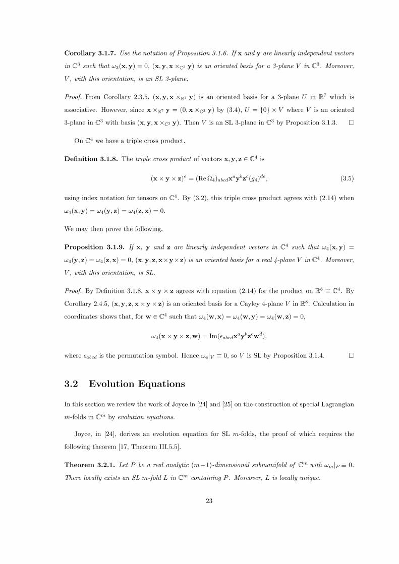
On C4 we have a triple cross product.
Definition 3.1.8. The triple cross product of vectors x,y, z ∈ C4 is
(x× y × z)e = (ReΩ4)abcdxaybzc(g4)de, (3.5)
using index notation for tensors on C4. By (3.2), this triple cross product agrees with (2.14) when
ω4(x,y) = ω4(y, z) = ω4(z,x) = 0.
We may then prove the following.
Proposition 3.1.9. If x, y and z are linearly independent vectors in C4 such that ω4(x,y) =
ω4(y, z) = ω4(z,x) = 0, (x,y, z,x×y×z) is an oriented basis for a real 4-plane V in C4. Moreover,
V , with this orientation, is SL.
Proof. By Definition 3.1.8, x × y × z agrees with equation (2.14) for the product on R8 ∼= C4. By
Corollary 2.4.5, (x,y, z,x× y× z) is an oriented basis for a Cayley 4-plane V in R8. Calculation in
coordinates shows that, for w ∈ C4 such that ω4(w,x) = ω4(w,y) = ω4(w, z) = 0,
ω4(x× y × z,w) = Im(εabcdxaybzcwd),
where εabcd is the permutation symbol. Hence ω4|V ≡ 0, so V is SL by Proposition 3.1.4.
3.2 Evolution Equations
In this section we review the work of Joyce in [24] and [25] on the construction of special Lagrangian
m-folds in Cm by evolution equations.
Joyce, in [24], derives an evolution equation for SL m-folds, the proof of which requires the
following theorem [17, Theorem III.5.5].
Theorem 3.2.1. Let P be a real analytic (m−1)-dimensional submanifold of Cm with ωm|P ≡ 0.
There locally exists an SL m-fold L in Cm containing P . Moreover, L is locally unique.
23

The use of the Cartan–Kahler Theorem in the proof of Theorem 3.2.1 necessitates the requirement
that P be real analytic. We now give a key result from [24], taken from [24, Theorem 3.3].
Theorem 3.2.2. Let P be a compact, orientable, (m−1)-dimensional, real analytic manifold, χ
a real analytic nowhere vanishing section of Λm−1TP and ψ : P → Cm a real analytic embedding
(immersion) such that ψ∗(ωm) ≡ 0 on P . There exist ε > 0 and a unique family ψt : t ∈ (−ε, ε)of real analytic maps ψt : P → Cm with ψ0 = ψ satisfying
(dψt
dt
)b
= (ψt)∗(χ)a1... am−1(ReΩm)a1... am−1am(gm)amb,
using index notation for tensors on Cm. Define Ψ : (−ε, ε) × P → Cm by Ψ(t, p) = ψt(p). Then
M = Image Ψ is a nonsingular embedded (immersed) SL m-fold in Cm.
In [25, §3] Joyce introduces the idea of affine evolution data with which he is able to derive an
evolution equation, and therefore reduces the infinite-dimensional problem of Theorem 3.2.2 to a
finite-dimensional one.
Definition 3.2.3. Let 2 ≤ m ≤ n be integers. A set of affine evolution data is a pair (P, χ), where
P is an (m−1)-dimensional submanifold of Rn and χ : Rn → Λm−1Rn is an affine map, such that
χ(p) is a nonzero element of Λm−1TP in Λm−1Rn for each nonsingular p ∈ P . We suppose also that
P is not contained in any proper affine subspace Rk of Rn.
Let Aff (Rn,Cm) be the affine space of affine maps ψ : Rn → Cm and define Cωm
P to be the set of
ψ ∈ Aff (Rn,Cm) satisfying:
(i) ψ∗(ωm)|P ≡ 0;
(ii) ψ|TpP : TpP → Cm is injective for all p in a dense open subset of P .
Then (i) is a quadratic condition on ψ and (ii) is an open condition on ψ, so Cωm
P is a nonempty
open set in the intersection of a finite number of quadrics in Aff (Rn,Cm).
The conditions upon χ in Definition 3.2.3 are strong. The result is that there are few known examples
of affine evolution data. The evolution equation derived in [25, Theorem 3.5] is given below.
Theorem 3.2.4. Let (P, χ) be a set of affine evolution data and let ψ ∈ Cωm
P , where Cωm
P is defined
in Definition 3.2.3. There exist ε > 0 and a unique real analytic family ψt : t ∈ (−ε, ε) in Cωm
P
with ψ0 = ψ, satisfying(
dψt
dt(x)
)b
= (ψt)∗(χ(x))a1... am−1(ReΩm)a1... am−1am(gm)amb
for all x ∈ Rn, using index notation for tensors in Cm. Moreover, M = ψt(p) : t ∈ (−ε, ε), p ∈ Pis an SL m-fold in Cm wherever it is nonsingular.
24
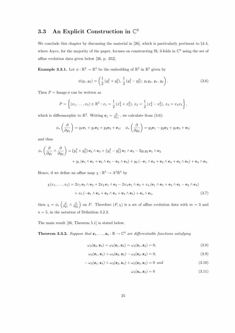
3.3 An Explicit Construction in C3
We conclude this chapter by discussing the material in [26], which is particularly pertinent to §4.4,
where Joyce, for the majority of the paper, focuses on constructing SL 3-folds in C3 using the set of
affine evolution data given below [26, p. 352].
Example 3.3.1. Let φ : R2 → R5 be the embedding of R2 in R5 given by
φ(y1, y2) =(
12
(y21 + y2
2),12
(y21 − y2
2), y1y2, y1, y2
). (3.6)
Then P = Image φ can be written as
P =
(x1, . . . , x5) ∈ R5 : x1 =12
(x24 + x2
5), x2 =12
(x24 − x2
5), x3 = x4x5
,
which is diffeomorphic to R2. Writing ej = ∂∂xj
, we calculate from (3.6):
φ∗
(∂
∂y1
)= y1e1 + y1e2 + y2e3 + e4; φ∗
(∂
∂y2
)= y2e1 − y2e2 + y1e3 + e5;
and thus
φ∗
(∂
∂y1∧ ∂
∂y2
)=
(y21 + y2
2
)e2 ∧ e3 +
(y21 − y2
2
)e1 ∧ e3 − 2y1y2 e1 ∧ e2
+ y1 (e1 ∧ e5 + e2 ∧ e5 − e3 ∧ e4) + y2 (−e1 ∧ e4 + e2 ∧ e4 + e3 ∧ e5) + e4 ∧ e5.
Hence, if we define an affine map χ : R5 → Λ2R5 by
χ(x1, . . . , x5) = 2x1 e2 ∧ e3 + 2x2 e1 ∧ e3 − 2x3 e1 ∧ e2 + x4 (e1 ∧ e5 + e2 ∧ e5 − e3 ∧ e4)
+ x5 (−e1 ∧ e4 + e2 ∧ e4 + e3 ∧ e5) + e4 ∧ e5, (3.7)
then χ = φ∗(
∂∂y1
∧ ∂∂y2
)on P . Therefore (P, χ) is a set of affine evolution data with m = 3 and
n = 5, in the notation of Definition 3.2.3.
The main result [26, Theorem 5.1] is stated below.
Theorem 3.3.2. Suppose that z1, . . . , z6 : R→ C3 are differentiable functions satisfying
ω3(z2, z3) = ω3(z1, z3) = ω3(z1, z2) = 0, (3.8)
ω3(z1, z5) + ω3(z2, z5)− ω3(z3, z4) = 0, (3.9)
− ω3(z1, z4) + ω3(z2, z4) + ω3(z3, z5) = 0 and (3.10)
ω3(z4, z5) = 0 (3.11)
25

at t = 0, and the equations:
dz1
dt= 2z2 × z3;
dz2
dt= 2z1 × z3;
dz3
dt= −2z1 × z2; (3.12)
dz4
dt= z1 × z5 + z2 × z5 − z3 × z4;
dz5
dt= −z1 × z4 + z2 × z4 + z3 × z5; and (3.13)
dz6
dt= z4 × z5 (3.14)
for all t ∈ R, where × is defined by (3.3). The subset M of C3 given by
M =
12
(y21 + y2
2) z1(t) +12
(y21 − y2
2) z2(t) + y1y2 z3(t) + y1 z4(t) + y2 z5(t) + z6(t) : y1, y2, t ∈ R
is a special Lagrangian 3-fold in C3 wherever it is nonsingular.
Joyce [26] solves (3.12)-(3.14) subject to the conditions (3.8)-(3.11), dividing the solutions into
sets based on the dimension of 〈z1(t), z2(t), z3(t)〉R for generic t ∈ R. Our concern shall lie with the
case dim 〈z1(t), z2(t), z3(t)〉R = 3, which forms the bulk of the results of [26]. The solutions here
involve the Jacobi elliptic functions: sn(u, k), cn(u, k) and dn(u, k) for k ∈ [0, 1]. A description of
these functions may be found in [10, Chapter VII].
The embedding given in Example 3.3.1 was constructed by considering the action of SL(2,R)nR2
on R2. Hence, Joyce [26, Proposition 9.1] shows that solutions of (3.12), satisfying the condition
(3.8), are equivalent under the natural actions of SL(2,R) and SU(3) to a solution z1 = (z1, 0, 0),
z2 = (0, z2, 0), z3 = (0, 0, z3), for differentiable functions z1, z2, z3 : R→ C. We therefore assume z1,
z2 and z3 are of this form. Equations (3.12) become
dz1
dt= 2 z2z3,
dz2
dt= −2 z3z1 and
dz3
dt= −2 z1z2. (3.15)
The next result is taken from [26, Proposition 9.2].
Proposition 3.3.3. Given any initial data, z1(0), z2(0) and z3(0), solutions to (3.15) exist for all
t ∈ R. Wherever the zj(t) are nonzero they may be written as:
2z1 = eiθ1
√α2
1 + v ; 2z2 = eiθ2
√α2
2 − v ; and 2z3 = eiθ3
√α2
3 − v,
where αj ∈ R for all j and v, θ1, θ2, θ3 : R → R are differentiable functions. Let θ = θ1 + θ2 + θ3
and let Q(v) = (α21 + v)(α2
2 − v)(α23 − v). There exists A ∈ R such that Q(v)
12 sin θ = A.
We conclude with the statement of a theorem [26, Theorem 9.3] that shall be of great use in §4.4.
Theorem 3.3.4. Use the notation of Proposition 3.3.3. Let αj > 0 for all j with α−21 = α−2
2 +α−23 .
Suppose that v has a minimum at t = 0, θ2(0) = θ3(0) = 0, A ≥ 0 and α2 ≤ α3. Exactly one of the
following four cases holds.
26

(i) A = 0, α2 = α3 and z1, z2, z3 are given by:
2z1(t) =√
3α1 tanh(√
3α1t)
and 2z2(t) = 2z3(t) =√
3α1 sech(√
3α1t)
.
(ii) A = 0, α2 < α3 and z1, z2, z3 are given by:
2z1(t) =√
α21 + α2
2 sn(σt, τ);
2z2(t) =√
α21 + α2
2 cn(σt, τ); and
2z3(t) =√
α21 + α2
3 dn(σt, τ),
where σ =√
α21 + α2
3 and τ =
√α2
1 + α22
α21 + α2
3
.
(iii) 0 < A < α1α2α3. Let the roots of Q(v)−A2 be γ1, γ2, γ3, ordered such that γ1 ≤ 0 ≤ γ2 ≤ γ3.
Then v, θ1, θ2, θ3 are given by:
v(t) = γ1 + (γ2 − γ1) sn2(σt, τ);
θ1(t) = θ1(0)−A
∫ t
0
ds
α21 + γ1 + (γ2 − γ1) sn2(σs, τ)
;
θ2(t) = A
∫ t
0
ds
α22 − γ1 − (γ2 − γ1) sn2(σs, τ)
; and
θ3(t) = A
∫ t
0
ds
α23 − γ1 − (γ2 − γ1) sn2(σs, τ)
,
where σ =√
γ3 − γ1 and τ =√
γ2 − γ1
γ3 − γ1.
(iv) A = α1α2α3. Define a1, a2, a3 ∈ R by:
a1 = −α2α3
α1; a2 =
α3α1
α2; and a3 =
α1α2
α3.
Then a1 + a2 + a3 = 0, since α−21 = α−2
2 + α−23 , and z1, z2, z3 are given by:
2z1(t) = iα1eia1t; 2z2(t) = α2e
ia2t; and 2z3(t) = α3eia3t.
27

Chapter 4
Associative 3-folds in R7
In this chapter we construct examples of associative 3-folds in R7 by three separate methods. The
first method, described in §4.2, produces 3-folds with symmetries using evolution equations. In §4.4
an affine evolution equation gives a 14-dimensional family of associative 3-folds. Finally, in §4.5, we
consider 1-ruled 3-folds. The material exhibited is a generalisation of the work of Joyce in [24], [25],
[26] and [27].
4.1 The First Evolution Equation
To derive our evolution equation we shall require two results related to real analyticity. The first is
an immediate corollary of Theorem 1.1.3.
Theorem 4.1.1. An associative 3-fold in R7 is real analytic wherever it is nonsingular.
The proof of the next result [17, Theorem IV.4.1] relies on the Cartan–Kahler Theorem, which is
only applicable in the real analytic category.
Theorem 4.1.2. Let P be a 2-dimensional real analytic submanifold of ImO ∼= R7. There locally
exists a real analytic associative 3-fold N in R7 which contains P . Moreover, N is locally unique.
We now formulate an evolution equation for associative 3-folds, given a 2-dimensional real ana-
lytic submanifold of R7, following Theorem 3.2.2.
Theorem 4.1.3. Let P be a compact, orientable, 2-dimensional, real analytic manifold, χ a real
analytic nowhere vanishing section of Λ2TP and ψ : P → R7 a real analytic embedding (immersion).
There exist ε > 0 and a unique family ψt : t ∈ (−ε, ε) of real analytic maps ψt : P → R7 with
ψ0 = ψ satisfying (dψt
dt
)d
= (ψt)∗(χ)ab(ϕ0)abc(g0)cd, (4.1)
28
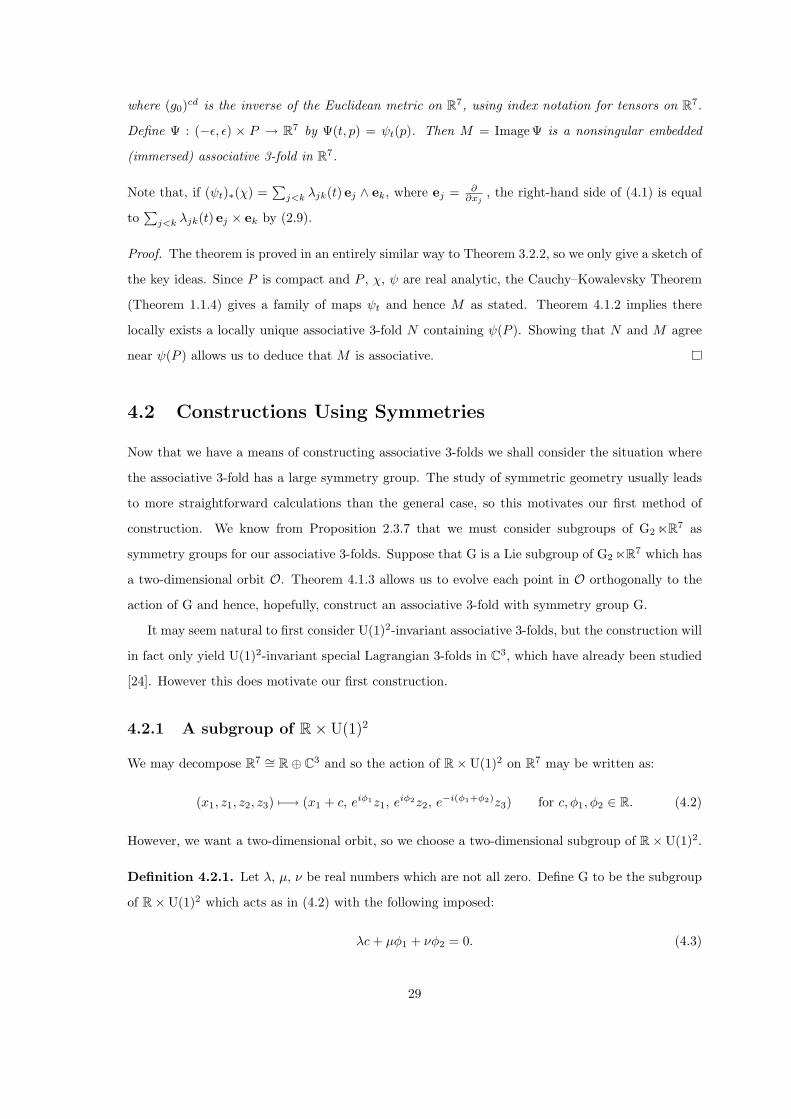
where (g0)cd is the inverse of the Euclidean metric on R7, using index notation for tensors on R7.
Define Ψ : (−ε, ε) × P → R7 by Ψ(t, p) = ψt(p). Then M = Image Ψ is a nonsingular embedded
(immersed) associative 3-fold in R7.
Note that, if (ψt)∗(χ) =∑
j<k λjk(t) ej ∧ ek, where ej = ∂∂xj
, the right-hand side of (4.1) is equal
to∑
j<k λjk(t) ej × ek by (2.9).
Proof. The theorem is proved in an entirely similar way to Theorem 3.2.2, so we only give a sketch of
the key ideas. Since P is compact and P , χ, ψ are real analytic, the Cauchy–Kowalevsky Theorem
(Theorem 1.1.4) gives a family of maps ψt and hence M as stated. Theorem 4.1.2 implies there
locally exists a locally unique associative 3-fold N containing ψ(P ). Showing that N and M agree
near ψ(P ) allows us to deduce that M is associative.
4.2 Constructions Using Symmetries
Now that we have a means of constructing associative 3-folds we shall consider the situation where
the associative 3-fold has a large symmetry group. The study of symmetric geometry usually leads
to more straightforward calculations than the general case, so this motivates our first method of
construction. We know from Proposition 2.3.7 that we must consider subgroups of G2nR7 as
symmetry groups for our associative 3-folds. Suppose that G is a Lie subgroup of G2nR7 which has
a two-dimensional orbit O. Theorem 4.1.3 allows us to evolve each point in O orthogonally to the
action of G and hence, hopefully, construct an associative 3-fold with symmetry group G.
It may seem natural to first consider U(1)2-invariant associative 3-folds, but the construction will
in fact only yield U(1)2-invariant special Lagrangian 3-folds in C3, which have already been studied
[24]. However this does motivate our first construction.
4.2.1 A subgroup of R× U(1)2
We may decompose R7 ∼= R⊕ C3 and so the action of R×U(1)2 on R7 may be written as:
(x1, z1, z2, z3) 7−→ (x1 + c, eiφ1z1, eiφ2z2, e−i(φ1+φ2)z3) for c, φ1, φ2 ∈ R. (4.2)
However, we want a two-dimensional orbit, so we choose a two-dimensional subgroup of R×U(1)2.
Definition 4.2.1. Let λ, µ, ν be real numbers which are not all zero. Define G to be the subgroup
of R×U(1)2 which acts as in (4.2) with the following imposed:
λc + µφ1 + νφ2 = 0. (4.3)
29

If µ = ν = 0 then G is U(1)2. Suppose µν 6= 0. If there exist coprime integers p and q such that
µp + νq = 0 then G is R×U(1) and otherwise it is an R2 subgroup.
Define smooth maps ψt : G → R7 by:
ψt(c, eiφ1 , eiφ2) = (x1(t) + c, eiφ1z1(t), eiφ2z2(t), e−i(φ1+φ2)z3(t)), (4.4)
where x1(t), z1(t) = x2(t) + ix3(t), z2(t) = x4(t) + ix5(t) and z3(t) = x6(t) + ix7(t) are smooth
functions of t.
Using (4.4) we calculate:
v1 = (ψt)∗
(∂
∂φ1
)= i
(z1
∂
∂z1− z1
∂
∂z1
)− i
(z3
∂
∂z3− z3
∂
∂z3
)
= x2∂
∂x3− x3
∂
∂x2− x6
∂
∂x7+ x7
∂
∂x6; (4.5)
v2 = (ψt)∗
(∂
∂φ2
)= i
(z2
∂
∂z2− z2
∂
∂z2
)− i
(z3
∂
∂z3− z3
∂
∂z3
)
= x4∂
∂x5− x5
∂
∂x4− x6
∂
∂x7+ x7
∂
∂x6; and (4.6)
v3 = (ψt)∗
(∂
∂c
)=
∂
∂x1, (4.7)
where z1 = x2 + ix3, z2 = x4 + ix5 and z3 = x6 + ix7. These three vectors are tangential to the
action of R×U(1)2; the vector v1 corresponds to a rotation of z1 by i and of z3 by −i, and similarly
for v2. The condition (4.3) corresponds to the choice of a nowhere vanishing section χ of Λ2TG:
χ = λ∂
∂φ1∧ ∂
∂φ2+ µ
∂
∂φ2∧ ∂
∂c+ ν
∂
∂c∧ ∂
∂φ1.
If we let u = v1 ∧ v2, v = v2 ∧ v3 and w = v3 ∧ v1 then
(ψt)∗(χ) = λu + µv + νw.
Therefore, using (4.5)-(4.7) and equation (2.6) for ϕ0 we find that, writing ej = ∂∂xj
,
(ψt)∗(χ)ab(ϕ0)abc(g0)cd =(λ(x5x7 − x4x6)− νx2
)e2 +
(λ(x5x6 + x4x7)− νx3
)e3
+(λ(x3x7 − x2x6) + µx4
)e4 +
(λ(x3x6 + x2x7) + µx5
)e5
+(λ(x3x5 − x2x4) + (ν − µ)x6
)e6 +
(λ(x3x4 + x2x5) + (ν − µ)x7
)e7. (4.8)
We also have thatdψt
dt=
7∑
j=1
dxj(t)dt
ej . (4.9)
Equating both sides of (4.1) using (4.8) and (4.9) and applying Theorem 4.1.3 provides the
following theorem.
30
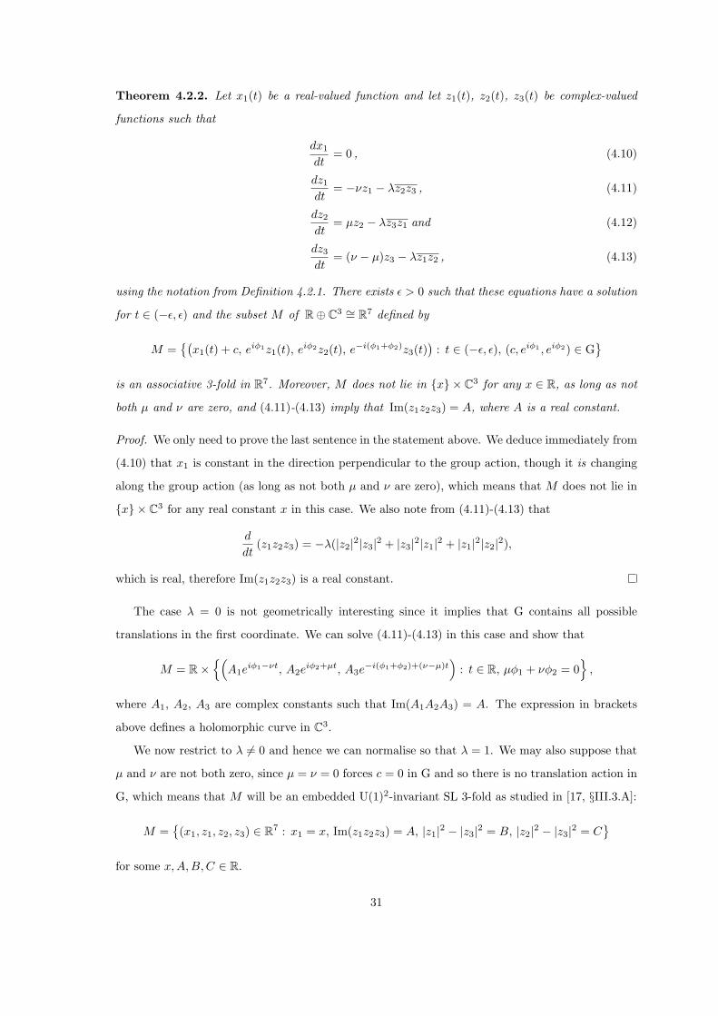
Theorem 4.2.2. Let x1(t) be a real-valued function and let z1(t), z2(t), z3(t) be complex-valued
functions such that
dx1
dt= 0 , (4.10)
dz1
dt= −νz1 − λz2z3 , (4.11)
dz2
dt= µz2 − λz3z1 and (4.12)
dz3
dt= (ν − µ)z3 − λz1z2 , (4.13)
using the notation from Definition 4.2.1. There exists ε > 0 such that these equations have a solution
for t ∈ (−ε, ε) and the subset M of R⊕ C3 ∼= R7 defined by
M =(
x1(t) + c, eiφ1z1(t), eiφ2z2(t), e−i(φ1+φ2)z3(t))
: t ∈ (−ε, ε), (c, eiφ1 , eiφ2) ∈ G
is an associative 3-fold in R7. Moreover, M does not lie in x × C3 for any x ∈ R, as long as not
both µ and ν are zero, and (4.11)-(4.13) imply that Im(z1z2z3) = A, where A is a real constant.
Proof. We only need to prove the last sentence in the statement above. We deduce immediately from
(4.10) that x1 is constant in the direction perpendicular to the group action, though it is changing
along the group action (as long as not both µ and ν are zero), which means that M does not lie in
x × C3 for any real constant x in this case. We also note from (4.11)-(4.13) that
d
dt(z1z2z3) = −λ(|z2|2|z3|2 + |z3|2|z1|2 + |z1|2|z2|2),
which is real, therefore Im(z1z2z3) is a real constant.
The case λ = 0 is not geometrically interesting since it implies that G contains all possible
translations in the first coordinate. We can solve (4.11)-(4.13) in this case and show that
M = R×(
A1eiφ1−νt, A2e
iφ2+µt, A3e−i(φ1+φ2)+(ν−µ)t
): t ∈ R, µφ1 + νφ2 = 0
,
where A1, A2, A3 are complex constants such that Im(A1A2A3) = A. The expression in brackets
above defines a holomorphic curve in C3.
We now restrict to λ 6= 0 and hence we can normalise so that λ = 1. We may also suppose that
µ and ν are not both zero, since µ = ν = 0 forces c = 0 in G and so there is no translation action in
G, which means that M will be an embedded U(1)2-invariant SL 3-fold as studied in [17, §III.3.A]:
M =(x1, z1, z2, z3) ∈ R7 : x1 = x, Im(z1z2z3) = A, |z1|2 − |z3|2 = B, |z2|2 − |z3|2 = C
for some x,A, B, C ∈ R.
31
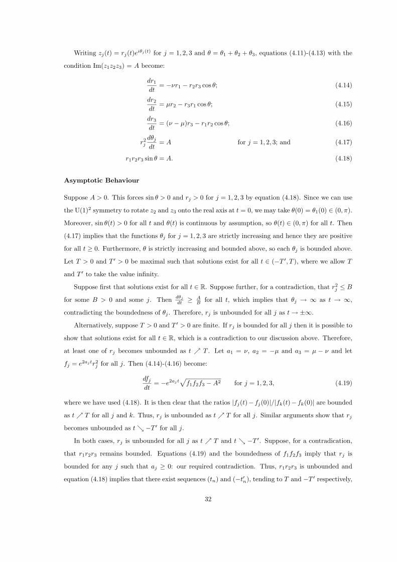
Writing zj(t) = rj(t)eiθj(t) for j = 1, 2, 3 and θ = θ1 + θ2 + θ3, equations (4.11)-(4.13) with the
condition Im(z1z2z3) = A become:
dr1
dt= −νr1 − r2r3 cos θ; (4.14)
dr2
dt= µr2 − r3r1 cos θ; (4.15)
dr3
dt= (ν − µ)r3 − r1r2 cos θ; (4.16)
r2j
dθj
dt= A for j = 1, 2, 3; and (4.17)
r1r2r3 sin θ = A. (4.18)
Asymptotic Behaviour
Suppose A > 0. This forces sin θ > 0 and rj > 0 for j = 1, 2, 3 by equation (4.18). Since we can use
the U(1)2 symmetry to rotate z2 and z3 onto the real axis at t = 0, we may take θ(0) = θ1(0) ∈ (0, π).
Moreover, sin θ(t) > 0 for all t and θ(t) is continuous by assumption, so θ(t) ∈ (0, π) for all t. Then
(4.17) implies that the functions θj for j = 1, 2, 3 are strictly increasing and hence they are positive
for all t ≥ 0. Furthermore, θ is strictly increasing and bounded above, so each θj is bounded above.
Let T > 0 and T ′ > 0 be maximal such that solutions exist for all t ∈ (−T ′, T ), where we allow T
and T ′ to take the value infinity.
Suppose first that solutions exist for all t ∈ R. Suppose further, for a contradiction, that r2j ≤ B
for some B > 0 and some j. Then dθj
dt ≥ AB for all t, which implies that θj → ∞ as t → ∞,
contradicting the boundedness of θj . Therefore, rj is unbounded for all j as t → ±∞.
Alternatively, suppose T > 0 and T ′ > 0 are finite. If rj is bounded for all j then it is possible to
show that solutions exist for all t ∈ R, which is a contradiction to our discussion above. Therefore,
at least one of rj becomes unbounded as t T . Let a1 = ν, a2 = −µ and a3 = µ − ν and let
fj = e2ajtr2j for all j. Then (4.14)-(4.16) become:
dfj
dt= −e2ajt
√f1f2f3 −A2 for j = 1, 2, 3, (4.19)
where we have used (4.18). It is then clear that the ratios |fj(t)− fj(0)|/|fk(t)− fk(0)| are bounded
as t T for all j and k. Thus, rj is unbounded as t T for all j. Similar arguments show that rj
becomes unbounded as t −T ′ for all j.
In both cases, rj is unbounded for all j as t T and t −T ′. Suppose, for a contradication,
that r1r2r3 remains bounded. Equations (4.19) and the boundedness of f1f2f3 imply that rj is
bounded for any j such that aj ≥ 0: our required contradiction. Thus, r1r2r3 is unbounded and
equation (4.18) implies that there exist sequences (tn) and (−t′n), tending to T and −T ′ respectively,
32

such that (sin θ(tn)) and (sin θ(−t′n)) are strictly decreasing sequences tending to 0. However, θ is
a strictly increasing function taking values in (0, π) and hence sin θ must be eventually decreasing
as t T and t −T ′. Therefore, sin θ → 0 as t T and t −T ′. We conclude that θ → π as
t T and θ → 0 as t −T ′. Moreover, r1r2r3 →∞ as t T and t −T ′.
The upshot of this analysis is that we can now write down the asymptotic differential equations.
Since cos θ → −1, the approximate equations as t T are thus:
dr1
dt= −νr1 + r2r3;
dr2
dt= µr2 + r3r1; and
dr3
dt= (ν − µ)r3 + r1r2.
Equations (4.19) imply that r1, r2 and r3 must eventually grow at the same rate as t T , so we
approximate further by neglecting the linear terms, which will be dominated by the quadratic parts
as t T , to give:
rjdrj
dt= r1r2r3 for j = 1, 2, 3.
These equations can be solved to show that, for t sufficiently near T , which must be finite,
rj ∼ 1T − t
for j = 1, 2, 3.
Hence the functions r1, r2 and r3 reach infinity in finite positive time. Similarly, since cos θ → 1 as
t −T ′ we deduce that T ′ must be finite and that, for t sufficiently near −T ′,
rj ∼ 1T ′ + t
for j = 1, 2, 3.
Hence the functions r1, r2 and r3 reach infinity in finite negative time.
We conclude that, at infinity, these associative 3-folds behave like the standard U(1)2-invariant
SL 3-fold as studied by Harvey and Lawson [17, §III.3.A]:
(z1, z2, z3) ∈ C3 : |z1| = |z2| = |z3|, Im(z1z2z3) = A, Re(z1z2z3) > 0.
This is the result expected since the translation component of the group action becomes negligible
in comparison to the U(1)2 action as r1, r2 and r3 become large.
4.2.2 U(1)-invariant cones
In this subsection we consider associative 3-folds which are invariant both under an action of U(1)
on the C3 component of R7 ∼= R⊕ C3, and under dilations.
Definition 4.2.3. Let R+ denote the group of positive real numbers under multiplication. The
group action of R+ ×U(1) on R7 ∼= R⊕ C3 is given by, for some fixed α1, α2, α3 ∈ R:
(x1, z1, z2, z3) 7−→ (rx1, reisα1z1, reisα2z2, reisα3z3) r > 0, s ∈ R.
33

To ensure we have a U(1) action in G2, we choose α1, α2, α3 to be coprime integers satisfying
α1 + α2 + α3 = 0.
Define smooth maps ψt : R+ ×U(1) → R7 by:
ψt(r, eis) = (rx1(t), reisα1z1(t), reisα2z2(t), reisα3z3(t)), (4.20)
where x1(t), z1(t) = x2(t) + ix3(t), z2(t) = x4(t) + ix5(t) and z3(t) = x6(t) + ix7(t) are smooth
functions of t.
Using (4.20) we calculate the tangent vectors to the group action given in Definition 4.2.3:
u = (ψt)∗
(∂
∂r
)=
7∑
j=1
xj∂
∂xjand
v = (ψt)∗
(∂
∂s
)= α1
(x2
∂
∂x3− x3
∂
∂x2
)+ α2
(x4
∂
∂x5− x5
∂
∂x4
)+ α3
(x6
∂
∂x7− x7
∂
∂x6
).
If we take χ = ∂∂r ∧ ∂
∂s then (ψt)∗(χ) = u ∧ v. We deduce that, writing ej = ∂∂xj
,
u× v =(α1(x2
2 + x23) + α2(x2
4 + x25) + α3(x2
6 + x27)
)e1
+(− α1x1x2 + (α2 − α3)(x4x7 + x5x6)
)e2 +
(− α1x1x3 + (α2 − α3)(x4x6 − x5x7))e3
+(− α2x1x4 + (α3 − α1)(x2x7 + x3x6)
)e4 +
(− α2x1x5 + (α3 − α1)(x2x6 − x3x7))e5
+(− α3x1x6 + (α1 − α2)(x2x5 + x3x4)
)e6 +
(− α3x1x7 + (α1 − α2)(x2x4 − x3x5))e7.
We also have thatdψt
dt=
7∑
j=1
dxj(t)dt
ej .
Equating both sides of (4.1) using the above formulae as in §4.2.1 we obtain the following theorem.
Theorem 4.2.4. Use the notation of Definition 4.2.3. Let β1 = α2 − α3, β2 = α3 − α1 and
β3 = α1 − α2. Let x1(t) be a real-valued function and let z1(t), z2(t), z3(t) be complex-valued
functions such that
dx1
dt= α1|z1|2 + α2|z2|2 + α3|z3|2, (4.21)
dz1
dt= −α1x1z1 + iβ1z2z3, (4.22)
dz2
dt= −α2x1z2 + iβ2z3z1 and (4.23)
dz3
dt= −α3x1z3 + iβ3z1z2. (4.24)
These equations have a solution for all t ∈ R and the subset M of R⊕ C3 ∼= R7 defined by
M =(
rx1(t), reisα1z1(t), reisα2z2(t), reisα3z3(t))
: r ∈ R+, s, t ∈ R
34

is an associative 3-fold in R7. Moreover, (4.21)-(4.24) imply that x21 + |z1|2 + |z2|2 + |z3|2 can be
chosen to be 1 and that Re(z1z2z3) = A, where A is a real constant.
Proof. Noting that β1 + β2 + β3 = 0, we immediately see that x21 + |z1|2 + |z2|2 + |z3|3 is a constant
which we can take to be one. This is hardly surprising since the associative 3-fold was constructed
so as to be a cone. We also see from (4.22)-(4.24) that
d
dt(z1z2z3) = i(β1|z2|2|z3|2 + β2|z3|2|z1|2 + β3|z1|2|z2|2),
which is purely imaginary, and therefore Re(z1z2z3) = A is a real constant.
The proof that (4.21)-(4.24) have solutions for all t ∈ R is deferred until later in the subsection.
Writing zj(t) = rj(t)eiθj(t) for j = 1, 2, 3 and θ = θ1 + θ2 + θ3, (4.21)-(4.24) become:
dx1
dt= α1r
21 + α2r
22 + α3r
23; (4.25)
dr1
dt= −α1x1r1 + β1r2r3 sin θ; (4.26)
dr2
dt= −α2x1r2 + β2r3r1 sin θ; (4.27)
dr3
dt= −α3x1r3 + β3r1r2 sin θ; and (4.28)
r2j
dθj
dt= βjA for j = 1, 2, 3, (4.29)
with the conditions
x21 + r2
1 + r22 + r2
3 = 1 and (4.30)
r1r2r3 cos θ = A. (4.31)
Unlike in §4.2.1, we are restricted in our choices of the real parameter A. The problem of
maximising A2, by (4.30) and (4.31), is equivalent to the problem of maximising r21r
22r
23 subject to
r21 +r2
2 +r23 = 1. By direct calculation the solution is r2
1 = r22 = r2
3 = 13 . Therefore A ∈
[− 1
3√
3, 1
3√
3
].
We can restrict to A ≥ 0 since changing the sign of A corresponds to reversing the sign of cos θ, so
the addition of π to θ.
The case where A = 13√
3is immediately soluble since this forces r1 = r2 = r3 = 1√
3, which
implies x1 = 0 by (4.30) and cos θ = 1 by (4.31), so we can take θ = 0. Equations (4.29) become
13
dθj
dt=
13√
3βj for j = 1, 2, 3,
which can easily be solved, along with the condition θ = 0, to give:
θj(t) =βj√3
t + γj for j = 1, 2, 3,
35
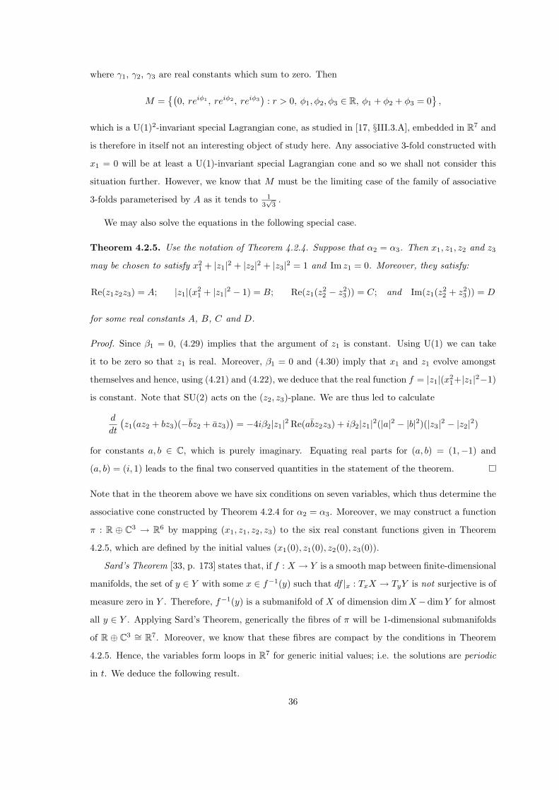
where γ1, γ2, γ3 are real constants which sum to zero. Then
M =(
0, reiφ1 , reiφ2 , reiφ3)
: r > 0, φ1, φ2, φ3 ∈ R, φ1 + φ2 + φ3 = 0
,
which is a U(1)2-invariant special Lagrangian cone, as studied in [17, §III.3.A], embedded in R7 and
is therefore in itself not an interesting object of study here. Any associative 3-fold constructed with
x1 = 0 will be at least a U(1)-invariant special Lagrangian cone and so we shall not consider this
situation further. However, we know that M must be the limiting case of the family of associative
3-folds parameterised by A as it tends to 13√
3.
We may also solve the equations in the following special case.
Theorem 4.2.5. Use the notation of Theorem 4.2.4. Suppose that α2 = α3. Then x1, z1, z2 and z3
may be chosen to satisfy x21 + |z1|2 + |z2|2 + |z3|2 = 1 and Im z1 = 0. Moreover, they satisfy:
Re(z1z2z3) = A; |z1|(x21 + |z1|2 − 1) = B; Re(z1(z2
2 − z23)) = C; and Im(z1(z2
2 + z23)) = D
for some real constants A, B, C and D.
Proof. Since β1 = 0, (4.29) implies that the argument of z1 is constant. Using U(1) we can take
it to be zero so that z1 is real. Moreover, β1 = 0 and (4.30) imply that x1 and z1 evolve amongst
themselves and hence, using (4.21) and (4.22), we deduce that the real function f = |z1|(x21+|z1|2−1)
is constant. Note that SU(2) acts on the (z2, z3)-plane. We are thus led to calculate
d
dt
(z1(az2 + bz3)(−bz2 + az3)
)= −4iβ2|z1|2 Re(abz2z3) + iβ2|z1|2(|a|2 − |b|2)(|z3|2 − |z2|2)
for constants a, b ∈ C, which is purely imaginary. Equating real parts for (a, b) = (1,−1) and
(a, b) = (i, 1) leads to the final two conserved quantities in the statement of the theorem.
Note that in the theorem above we have six conditions on seven variables, which thus determine the
associative cone constructed by Theorem 4.2.4 for α2 = α3. Moreover, we may construct a function
π : R ⊕ C3 → R6 by mapping (x1, z1, z2, z3) to the six real constant functions given in Theorem
4.2.5, which are defined by the initial values (x1(0), z1(0), z2(0), z3(0)).
Sard’s Theorem [33, p. 173] states that, if f : X → Y is a smooth map between finite-dimensional
manifolds, the set of y ∈ Y with some x ∈ f−1(y) such that df |x : TxX → TyY is not surjective is of
measure zero in Y . Therefore, f−1(y) is a submanifold of X of dimension dim X −dim Y for almost
all y ∈ Y . Applying Sard’s Theorem, generically the fibres of π will be 1-dimensional submanifolds
of R ⊕ C3 ∼= R7. Moreover, we know that these fibres are compact by the conditions in Theorem
4.2.5. Hence, the variables form loops in R7 for generic initial values; i.e. the solutions are periodic
in t. We deduce the following result.
36

Theorem 4.2.6. Use the notation of Theorem 4.2.4 and suppose that α2 = α3. For generic values
of the functions x1, z1, z2 and z3 at t = 0, the associative 3-folds constructed by Theorem 4.2.4 are
closed U(1)-invariant cones over T 2 in R7.
Domain of Definition
Theorem 4.1.3 gives us that a solution to (4.21)-(4.24) in Theorem 4.2.4 exists for sufficiently small
values of t, but we want to be able to say more about the domain of the solutions.
Rewriting (4.25)-(4.29) using y = r1r2r3 sin θ and sj = r2j for j = 1, 2, 3:
dx1
dt=
3∑
j=1
αjsj ;dsj
dt= −2αjx1sj + 2βjy for j = 1, 2, 3; and
dy
dt= β1s2s3 + β2s3s1 + β3s1s2.
(4.32)
Using (4.30) and (4.31), the solutions to (4.32) lie on the manifold
NA = (x1, s1, s2, s3, y) : x21 + s1 + s2 + s3 = 1, A2 + y2 = s1s2s3, s1, s2, s3 ≥ 0.
If we write x = (x1, s1, s2, s3, y), (4.32) can be cast in the form
dxdt
= f(x)
for some appropriate function f : R5 → R5. It is clear that f is continuous on NA, and since the
solution lies in NA it follows that f is bounded on NA, as NA is a closed and bounded and hence
compact subset of R5. Moreover, f will be bounded on a sufficiently small open neighbourhood U
of NA. We may then multiply f by a smooth bump function which takes the value one on NA and
is zero outside of U . We have thus constructed a function which equals f on NA and is continuous
and bounded on R5. We are then able to apply a result from the theory of ordinary differential
equations taken from [11, p. 53] after a couple of definitions also taken from [11].
Definition 4.2.7. Given a solution x(t) to an ordinary differential equation defined on an interval
(a, b), an extension is another solution x(t) defined on (c, d) ⊇ (a, b) which equals x(t) on (a, b).
Definition 4.2.8. A solution x(t) to an ordinary differential equation defined on an interval (a, b)
is maximal if for any extension x(t) which is defined on (c, d) then (a, b) = (c, d), hence x = x.
Theorem 4.2.9. Suppose f is continuous on (t,x)-space and that f is bounded. Any maximal
solution x(t) to the equationdxdt
= f(t,x)
has the t-axis as its domain.
37

Therefore, since we can find maximal solutions to equations (4.32), they must be defined for
all t ∈ R, and hence there exist solutions to (4.21)-(4.24) defined for all t ∈ R. This provides the
missing detail in the proof of Theorem 4.2.4.
4.3 The Second Evolution Equation
In general it is difficult to use Theorem 4.1.3 as stated to construct associative 3-folds since it is an
infinite-dimensional evolution problem. We follow the material in [25, §3] to reduce the theorem to
a finite-dimensional problem.
Definition 4.3.1. Let (P, χ) be a set of affine evolution data, in the sense of Definition 3.2.3, for
m = 3 and some n ≥ 3. Let Aff (Rn,R7) be the affine space of affine maps ψ : Rn → R7. Define
CP as the set of ψ ∈ Aff (Rn,R7) such that ψ|TpP : TpP → R7 is injective for all p in a dense open
subset of P . Let V be an associative 3-plane in R7. Generic linear maps ψ : Rn → V will satisfy
the condition to be members of CP . Hence CP is non-empty.
We formulate our second evolution equation following Theorem 3.2.4.
Theorem 4.3.2. Let (P, χ) be a set of affine evolution data and n, Aff (Rn,R7) and CP be as in
Definition 4.3.1. Suppose ψ ∈ CP . There exist ε > 0 and a unique real analytic family ψt : t ∈(−ε, ε) ⊆ CP with ψ0 = ψ satisfying
(dψt
dt(x)
)d
= (ψt)∗(χ(x))ab(ϕ0)abc(g0)cd (4.33)
for all x ∈ Rn. Define Ψ : (−ε, ε)×P → R7 by Ψ(t, p) = ψt(p). Then M = Image Ψ is an associative
3-fold wherever it is nonsingular.
Proof. As for Theorem 4.1.3, the proof is almost identical to the special Lagrangian case (Theorem
3.2.4), so we omit the details. Since (4.33) is of the form dψt
dt = Q(ψt) where Q is a quadratic, the
Cauchy–Picard Theorem [11, p. 14] of ordinary differential equations gives existence and uniqueness
of the family of maps stated. The proof then mirrors that of Theorem 3.2.2, noting that we can
drop the compactness condition for P since it was only needed previously to establish the existence
of the maps ψt. Finally, ψt ∈ CP for t sufficiently small since ψ0 ∈ CP and the condition to lie in CP
is an open one.
Before we construct associative 3-folds using this result, it is worth noting that using quadrics
to provide affine evolution data as in [25] would not be a worthwhile enterprise. Suppose Q ⊆ R3 is
a quadric and that L : R3 → R7 is a linear map. Then we can transform R7 using G2 such that, if
38
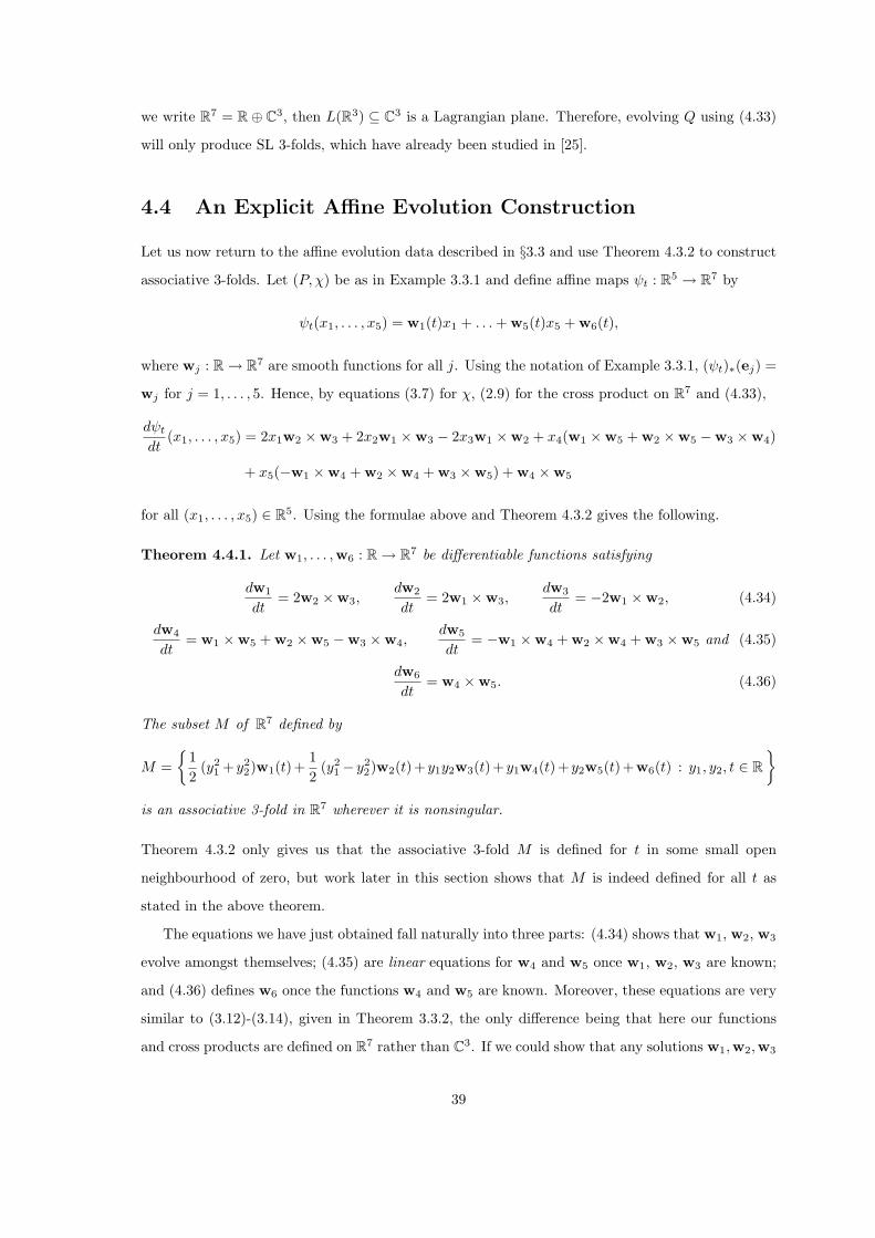
we write R7 = R⊕ C3, then L(R3) ⊆ C3 is a Lagrangian plane. Therefore, evolving Q using (4.33)
will only produce SL 3-folds, which have already been studied in [25].
4.4 An Explicit Affine Evolution Construction
Let us now return to the affine evolution data described in §3.3 and use Theorem 4.3.2 to construct
associative 3-folds. Let (P, χ) be as in Example 3.3.1 and define affine maps ψt : R5 → R7 by
ψt(x1, . . . , x5) = w1(t)x1 + . . . + w5(t)x5 + w6(t),
where wj : R→ R7 are smooth functions for all j. Using the notation of Example 3.3.1, (ψt)∗(ej) =
wj for j = 1, . . . , 5. Hence, by equations (3.7) for χ, (2.9) for the cross product on R7 and (4.33),
dψt
dt(x1, . . . , x5) = 2x1w2 ×w3 + 2x2w1 ×w3 − 2x3w1 ×w2 + x4(w1 ×w5 + w2 ×w5 −w3 ×w4)
+ x5(−w1 ×w4 + w2 ×w4 + w3 ×w5) + w4 ×w5
for all (x1, . . . , x5) ∈ R5. Using the formulae above and Theorem 4.3.2 gives the following.
Theorem 4.4.1. Let w1, . . . ,w6 : R→ R7 be differentiable functions satisfying
dw1
dt= 2w2 ×w3,
dw2
dt= 2w1 ×w3,
dw3
dt= −2w1 ×w2, (4.34)
dw4
dt= w1 ×w5 + w2 ×w5 −w3 ×w4,
dw5
dt= −w1 ×w4 + w2 ×w4 + w3 ×w5 and (4.35)
dw6
dt= w4 ×w5. (4.36)
The subset M of R7 defined by
M =
12
(y21 + y2
2)w1(t)+12
(y21 − y2
2)w2(t)+ y1y2w3(t)+ y1w4(t)+ y2w5(t)+w6(t) : y1, y2, t ∈ R
is an associative 3-fold in R7 wherever it is nonsingular.
Theorem 4.3.2 only gives us that the associative 3-fold M is defined for t in some small open
neighbourhood of zero, but work later in this section shows that M is indeed defined for all t as
stated in the above theorem.
The equations we have just obtained fall naturally into three parts: (4.34) shows that w1, w2, w3
evolve amongst themselves; (4.35) are linear equations for w4 and w5 once w1, w2, w3 are known;
and (4.36) defines w6 once the functions w4 and w5 are known. Moreover, these equations are very
similar to (3.12)-(3.14), given in Theorem 3.3.2, the only difference being that here our functions
and cross products are defined on R7 rather than C3. If we could show that any solutions w1,w2,w3
39

are equivalent to functions z1, z2, z3, lying in C3, satisfying (3.8) and (3.12), then we would be able
to use results from [26] to hopefully construct associative 3-folds which are not SL 3-folds. It is to
this end that we now proceed.
Suppose that w1(t),w2(t),w3(t) are solutions to (4.34). Let wj = wj(0) for all j and let
v = [w1, w2, w3], as defined by (2.10).
If v = 0, then, by Proposition 2.3.4, 〈w1, w2, w3〉R lies in an associative 3-plane which we can map
to R3 ⊆ C3 ⊆ R7 ∼= R⊕ C3, since G2 acts transitively on associative 3-planes [17, Theorem IV.1.8].
Let z1, z2, z3 be the images of w1, w2, w3 under this transformation and let ω3 be the standard
symplectic form on C3, given in Definition 3.1.1. Then z1, z2, z3 lie in R3 ⊆ C3 and so ω3(zj , zk) = 0
for j 6= k.
If v 6= 0, then v is orthogonal to wj for all j by Proposition 2.1.4, so we can split R7 ∼= R ⊕ C3
where R = 〈v〉 and C3 = 〈v〉⊥. Hence, wj lies in C3 for all j with respect to this splitting. By
Proposition 2.1.4, v is orthogonal to [wj , wk] = wjwk −wkwj = 2wj ×wk and therefore, from (2.8),
(ϕ0)abcvawj
bwkc = 0.
Using (3.1), we calculate (ϕ0)abcva = |v|(ω3)bc and hence, since |v| 6= 0, ω3(wj , wk) = 0.
We have shown that, using a G2 transformation, we can map the solutions w1(t),w2(t),w3(t)
to solutions z1(t), z2(t), z3(t) such that zj(0) ∈ C3 ⊆ R7 and ω3(zj(0), zk(0)) = 0. Our remarks
above about (4.34) and the relationship (3.4) between the cross products on C3 and R7 show that
z1(t), z2(t), z3(t) must remain in C3 and satisfy (3.12) along with condition (3.8). Hence, any solution
of (4.34) is equivalent up to a G2 transformation to a solution to the corresponding equations in
Theorem 3.3.2.
We now perform a parameter count in order to calculate the dimension of the family of associative
3-folds constructed by Theorem 4.4.1. The initial data w1(0), . . . ,w6(0) has 42 real parameters,
which implies that dim CP = 42, using the notation of Definition 4.3.1, so the family of curves in
CP has dimension 41, which corresponds to factoring out translation in t. It is shown in [26] that
GL(2,R)n R2 acts on this family of curves and, because of the internal symmetry of the evolution
data, any two curves related by this group action give the same 3-fold. Therefore we have to reduce
the dimension of distinct associative 3-folds up to this group action by 6 to 35. We can also identify
any two associative 3-folds which are isomorphic under automorphisms of R7, i.e. up to the action
of G2 nR7, so we reduce the dimension by 21 to 14.
In conclusion, the family of associative 3-folds constructed in this section has dimension 14,
whereas the dimension of the family of SL 3-folds constructed in Theorem 3.3.2 has dimension 9
40

by a similar parameter count. Thus, not only do we know that we have constructed new geometric
objects, but also how many more interesting parameters we expect to find.
4.4.1 Singularities
We study the singularities of the 3-folds constructed by Theorem 4.4.1 by introducing the function
F : R3 → R7 defined by:
F (y1, y2, t) = 12 (y2
1 + y22)w1(t) + 1
2 (y21 − y2
2)w2(t) + y1y2w3(t) + y1w4(t) + y2w5(t) + w6(t). (4.37)
Clearly, F is smooth and, if dF |(y1,y2,t) : R3 → R7 is injective for all (y1, y2, t) ∈ R, then F is an
immersion and M = Image F is nonsingular. Therefore the possible singularities of M correspond
to points where dF is not injective. Since we have from (4.34)-(4.36) that
∂F
∂y1× ∂F
∂y2=
∂F
∂t,
∂F∂t is perpendicular to the other two partial derivatives by (2.8) and it is zero if and only if the
y1 and y2 partial derivatives are linearly dependent by Proposition 2.1.7. We deduce that F is an
immersion if and only if ∂F∂y1
and ∂F∂y2
are linearly independent, since dF is injective if and only if the
three partial derivatives of F are linearly independent. The condition for F to be an immersion at
(0, 0, 0) is therefore that w4(0) and w5(0) are linearly independent.
We perform a parameter count for the family of singular associative 3-folds constructed by
Theorem 4.4.1. The set of initial data w1(0), . . . ,w6(0), with w4(0) and w5(0) linearly dependent,
has dimension 28 + 8 = 36, since the set of linearly dependent pairs in R7 has dimension 8. We
saw in the earlier parameter count above that the set of initial data without any restrictions had
dimension 42. Hence, the condition that F is not an immersion at (0, 0, 0) is of real codimension 6,
but this is clearly true for any point in R3 and therefore it is expected that the family of singular
associative 3-folds will be of codimension 6−3 = 3 in the family of all associative 3-folds constructed
by Theorem 4.4.1. Therefore the family of distinct singular associative 3-folds up to automorphisms
of R7 should have dimension 14− 3 = 11. Thus generic associative 3-folds constructed by Theorem
4.4.1 will be nonsingular. Moreover, the dimension of the family of singular associative 3-folds is
greater than the dimension of the family of singular SL 3-folds constructed from the same evolution
data, which has dimension 8 by a similar count.
We now model M = Image F near a singular point, which we take to be the origin without loss of
generality. Therefore, we expand w1(t), . . . ,w6(t) about t = 0 to study the singularity. Since dF is
not injective at the origin, w4(0) and w5(0) are linearly dependent. As mentioned above, Joyce [26,
41
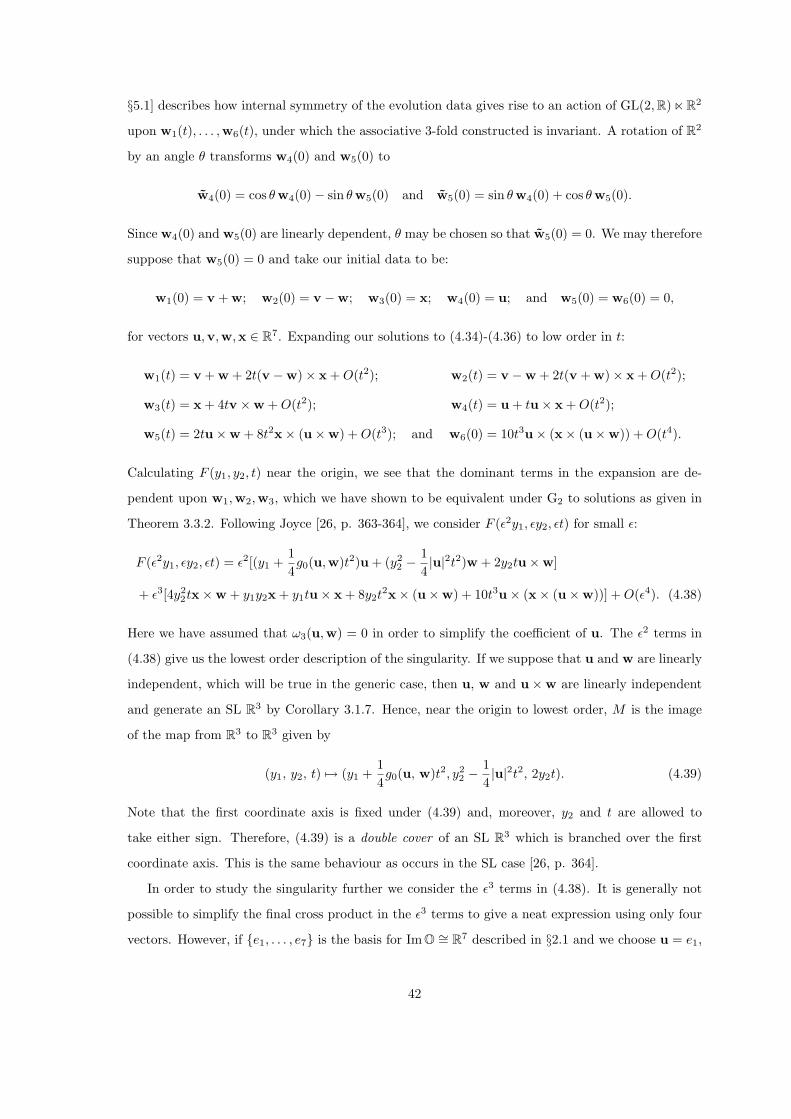
§5.1] describes how internal symmetry of the evolution data gives rise to an action of GL(2,R)nR2
upon w1(t), . . . ,w6(t), under which the associative 3-fold constructed is invariant. A rotation of R2
by an angle θ transforms w4(0) and w5(0) to
w4(0) = cos θ w4(0)− sin θ w5(0) and w5(0) = sin θ w4(0) + cos θ w5(0).
Since w4(0) and w5(0) are linearly dependent, θ may be chosen so that w5(0) = 0. We may therefore
suppose that w5(0) = 0 and take our initial data to be:
w1(0) = v + w; w2(0) = v −w; w3(0) = x; w4(0) = u; and w5(0) = w6(0) = 0,
for vectors u,v,w,x ∈ R7. Expanding our solutions to (4.34)-(4.36) to low order in t:
w1(t) = v + w + 2t(v −w)× x + O(t2); w2(t) = v −w + 2t(v + w)× x + O(t2);
w3(t) = x + 4tv ×w + O(t2); w4(t) = u + tu× x + O(t2);
w5(t) = 2tu×w + 8t2x× (u×w) + O(t3); and w6(0) = 10t3u× (x× (u×w)) + O(t4).
Calculating F (y1, y2, t) near the origin, we see that the dominant terms in the expansion are de-
pendent upon w1,w2,w3, which we have shown to be equivalent under G2 to solutions as given in
Theorem 3.3.2. Following Joyce [26, p. 363-364], we consider F (ε2y1, εy2, εt) for small ε:
F (ε2y1, εy2, εt) = ε2[(y1 +14g0(u,w)t2)u + (y2
2 −14|u|2t2)w + 2y2tu×w]
+ ε3[4y22tx×w + y1y2x + y1tu× x + 8y2t
2x× (u×w) + 10t3u× (x× (u×w))] + O(ε4). (4.38)
Here we have assumed that ω3(u,w) = 0 in order to simplify the coefficient of u. The ε2 terms in
(4.38) give us the lowest order description of the singularity. If we suppose that u and w are linearly
independent, which will be true in the generic case, then u, w and u×w are linearly independent
and generate an SL R3 by Corollary 3.1.7. Hence, near the origin to lowest order, M is the image
of the map from R3 to R3 given by
(y1, y2, t) 7→ (y1 +14g0(u, w)t2, y2
2 −14|u|2t2, 2y2t). (4.39)
Note that the first coordinate axis is fixed under (4.39) and, moreover, y2 and t are allowed to
take either sign. Therefore, (4.39) is a double cover of an SL R3 which is branched over the first
coordinate axis. This is the same behaviour as occurs in the SL case [26, p. 364].
In order to study the singularity further we consider the ε3 terms in (4.38). It is generally not
possible to simplify the final cross product in the ε3 terms to give a neat expression using only four
vectors. However, if e1, . . . , e7 is the basis for ImO ∼= R7 described in §2.1 and we choose u = e1,
42

w = e2 and x = e4, we can calculate each of the vectors appearing in (4.38) explicitly. Thus, in this
case, the next order of the singularity is the image of the following map from R3 to R7:
(y1, y2, t) 7→ (y1, y22 −
14
t2, 2y2t, εy1y2, εy1t, −4εy22t− 10εt3, 8εy2t
2).
Note that the singularity does not lie within C3 ⊆ R7 and so we have a model for a singularity which
is different from the SL case.
4.4.2 Solving the equations
From the work above, any solution w1(t),w2(t),w3(t) in R7 to (4.34) is equivalent under a G2
transformation to a solution z1(t), z2(t), z3(t) in C3 to (3.12) satisfying (3.8). We can thus use
results from [26] to produce some associative 3-folds. However, we must exercise some caution: we
require that 〈z1(t), z2(t), z3(t) : t ∈ R〉R = C3. If this does not occur, there may be a further G2
transformation that preserves the subspace spanned by the zj(t), but transforms C3 so that w4 and
w5 are mapped into C3, and thus the submanifold constructed will be an SL 3-fold embedded in R7.
When dim 〈z1(t), z2(t), z3(t)〉R < 3, for generic t ∈ R, the zj(t) define a subspace of an SL R3
in C3, which corresponds to an associative R3 in R7 by Proposition 3.1.3. The subgroup of G2
preserving an associative R3 is SO(4) [17, Theorem IV.1.8], and the subgroup of SU(3), which is
the automorphism group of C3, preserving the standard R3 is SO(3). Hence, the family of different
ways of identifying R7 ∼= R⊕C3 such that 〈z1(t), z2(t), z3(t)〉R is mapped into the standard R3 in C3
contains SO(4)/ SO(3) ∼= S3. We therefore have sufficient freedom left in using the G2 symmetry,
after mapping w1,w2,w3 into C3, to map w4 and w5 into C3 as well. This means that these cases
will only produce SL 3-folds.
It is also true in (i) and (ii) of Theorem 3.3.4 that the solutions zj(t) define a subspace of an SL
R3 in C3 and so these cases will not provide any new associative 3-folds either. Therefore we need
only consider (iii) and (iv) in Theorem 3.3.4.
Suppose we are in the situation of Theorem 3.3.4 so that, if we write R7 ∼= R ⊕ C3, w1 =
(0, w1, 0, 0), w2 = (0, 0, w2, 0) and w3 = (0, 0, 0, w3) for differentiable functions w1, w2, w3 : R →C. Let w4 = (y, p1, p2, q3) and w5 = (−x, q1,−q2, p3), where all the functions defined here are
differentiable. Equations (4.35) become
dx
dt= Im(w1p1 − w2p2 − w3p3), (4.40)
dp1
dt= ixw1 + w2p3 + w3p2,
dp2
dt= ixw2 − w3p1 − w1p3,
dp3
dt= ixw3 − w1p2 − w2p1; (4.41)
43
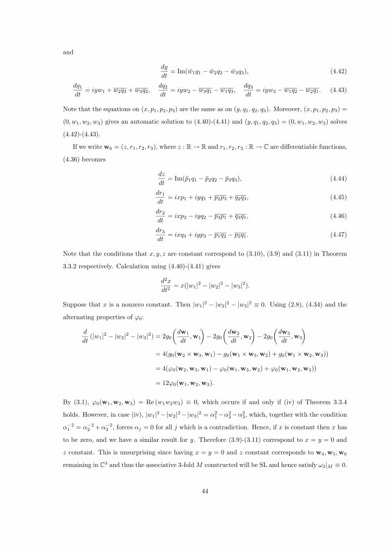
and
dy
dt= Im(w1q1 − w2q2 − w3q3), (4.42)
dq1
dt= iyw1 + w2q3 + w3q2,
dq2
dt= iyw2 − w3q1 − w1q3,
dq3
dt= iyw3 − w1q2 − w2q1. (4.43)
Note that the equations on (x, p1, p2, p3) are the same as on (y, q1, q2, q3). Moreover, (x, p1, p2, p3) =
(0, w1, w2, w3) gives an automatic solution to (4.40)-(4.41) and (y, q1, q2, q3) = (0, w1, w2, w3) solves
(4.42)-(4.43).
If we write w6 = (z, r1, r2, r3), where z : R→ R and r1, r2, r3 : R→ C are differentiable functions,
(4.36) becomes
dz
dt= Im(p1q1 − p2q2 − p3q3), (4.44)
dr1
dt= ixp1 + iyq1 + p2p3 + q2q3, (4.45)
dr2
dt= ixp2 − iyq2 − p3p1 + q3q1, (4.46)
dr3
dt= ixq3 + iyp3 − p1q2 − p2q1. (4.47)
Note that the conditions that x, y, z are constant correspond to (3.10), (3.9) and (3.11) in Theorem
3.3.2 respectively. Calculation using (4.40)-(4.41) gives
d2x
dt2= x(|w1|2 − |w2|2 − |w3|2).
Suppose that x is a nonzero constant. Then |w1|2 − |w2|2 − |w3|2 ≡ 0. Using (2.8), (4.34) and the
alternating properties of ϕ0:
d
dt(|w1|2 − |w2|2 − |w3|2) = 2g0
(dw1
dt,w1
)− 2g0
(dw2
dt,w2
)− 2g0
(dw3
dt,w3
)
= 4(g0(w2 ×w3,w1)− g0(w1 ×w3,w2) + g0(w1 ×w2,w3))
= 4(ϕ0(w2,w3,w1)− ϕ0(w1,w3,w2) + ϕ0(w1,w2,w3))
= 12ϕ0(w1,w2,w3).
By (3.1), ϕ0(w1,w2,w3) = Re (w1w2w3) ≡ 0, which occurs if and only if (iv) of Theorem 3.3.4
holds. However, in case (iv), |w1|2−|w2|2−|w3|2 = α21−α2
2−α23, which, together with the condition
α−21 = α−2
2 +α−23 , forces αj = 0 for all j which is a contradiction. Hence, if x is constant then x has
to be zero, and we have a similar result for y. Therefore (3.9)-(3.11) correspond to x = y = 0 and
z constant. This is unsurprising since having x = y = 0 and z constant corresponds to w4,w5,w6
remaining in C3 and thus the associative 3-fold M constructed will be SL and hence satisfy ω3|M ≡ 0.
44
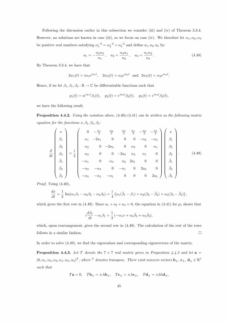
Following the discussion earlier in this subsection we consider (iii) and (iv) of Theorem 3.3.4.
However, no solutions are known in case (iii), so we focus on case (iv). We therefore let α1, α2, α3
be positive real numbers satisfying α−21 = α−2
2 + α−23 and define a1, a2, a3 by:
a1 = −α2α3
α1, a2 =
α3α1
α2, a3 =
α1α2
α3. (4.48)
By Theorem 3.3.4, we have that
2w1(t) = iα1eia1t, 2w2(t) = α2e
ia2t and 2w3(t) = α3eia3t.
Hence, if we let β1, β1, β3 : R→ C be differentiable functions such that
p1(t) = ieia1tβ1(t), p2(t) = eia2tβ2(t), p3(t) = eia3tβ3(t),
we have the following result.
Proposition 4.4.2. Using the notation above, (4.40)-(4.41) can be written as the following matrix
equation for the functions x, β1, β2, β3:
d
dt
x
β1
β2
β3
β1
β2
β3
=i
2
0 −α12
α22
α32
α12 −α2
2 −α32
α1 −2a1 0 0 0 −α3 −α2
α2 0 −2a2 0 α3 0 α1
α3 0 0 −2a3 α2 α1 0
−α1 0 α3 α2 2a1 0 0
−α2 −α3 0 −α1 0 2a2 0
−α3 −α2 −α1 0 0 0 2a3
x
β1
β2
β3
β1
β2
β3
. (4.49)
Proof. Using (4.40),
dx
dt=
12
Im(α1β1 − α2β2 − α3β3) =i
4(α1(β1 − β1) + α2(β2 − β2) + α3(β3 − β3)
),
which gives the first row in (4.49). Since a1 + a2 + a3 = 0, the equation in (4.41) for p1 shows that
idβ1
dt− a1β1 =
12
(−α1x + α2β3 + α3β2),
which, upon rearrangement, gives the second row in (4.49). The calculation of the rest of the rows
follows in a similar fashion.
In order to solve (4.49), we find the eigenvalues and corresponding eigenvectors of the matrix.
Proposition 4.4.3. Let T denote the 7 × 7 real matrix given in Proposition 4.4.2 and let a =
(0, α1, α2, α3, α1, α2, α3)T, where T denotes transpose. There exist nonzero vectors b±, c±, d± ∈ R7
such that
Ta = 0, Tb± = ±λb±, Tc± = ±λc±, Td± = ±3λd±,
45
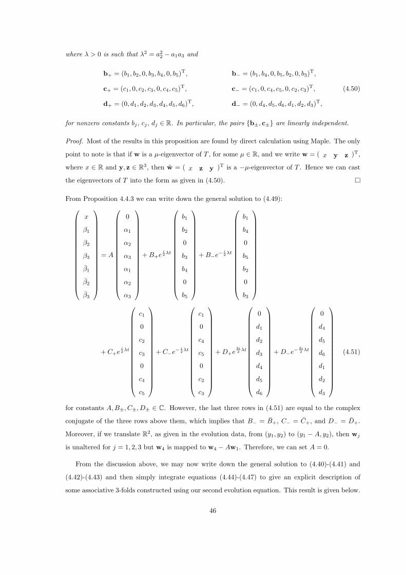
where λ > 0 is such that λ2 = a22 − a1a3 and
b+ = (b1, b2, 0, b3, b4, 0, b5)T, b− = (b1, b4, 0, b5, b2, 0, b3)T,
c+ = (c1, 0, c2, c3, 0, c4, c5)T, c− = (c1, 0, c4, c5, 0, c2, c3)T, (4.50)
d+ = (0, d1, d2, d3, d4, d5, d6)T, d− = (0, d4, d5, d6, d1, d2, d3)T,
for nonzero constants bj , cj , dj ∈ R. In particular, the pairs b±, c± are linearly independent.
Proof. Most of the results in this proposition are found by direct calculation using Maple. The only
point to note is that if w is a µ-eigenvector of T , for some µ ∈ R, and we write w = ( x y z )T,
where x ∈ R and y, z ∈ R3, then w = ( x z y )T is a −µ-eigenvector of T . Hence we can cast
the eigenvectors of T into the form as given in (4.50).
From Proposition 4.4.3 we can write down the general solution to (4.49):
x
β1
β2
β3
β1
β2
β3
= A
0
α1
α2
α3
α1
α2
α3
+ B+ei2 λt
b1
b2
0
b3
b4
0
b5
+ B−e−i2 λt
b1
b4
0
b5
b2
0
b3
+ C+ei2 λt
c1
0
c2
c3
0
c4
c5
+ C−e−i2 λt
c1
0
c4
c5
0
c2
c3
+ D+e3i2 λt
0
d1
d2
d3
d4
d5
d6
+ D−e−3i2 λt
0
d4
d5
d6
d1
d2
d3
(4.51)
for constants A,B±, C±, D± ∈ C. However, the last three rows in (4.51) are equal to the complex
conjugate of the three rows above them, which implies that B− = B+, C− = C+, and D− = D+.
Moreover, if we translate R2, as given in the evolution data, from (y1, y2) to (y1 − A, y2), then wj
is unaltered for j = 1, 2, 3 but w4 is mapped to w4 −Aw1. Therefore, we can set A = 0.
From the discussion above, we may now write down the general solution to (4.40)-(4.41) and
(4.42)-(4.43) and then simply integrate equations (4.44)-(4.47) to give an explicit description of
some associative 3-folds constructed using our second evolution equation. This result is given below.
46

Theorem 4.4.4. Define functions x, y, z : R→ R and wj , pj , qj , rj : R→ C for j = 1, 2, 3 by:
2w1(t) = iα1eia1t, 2w2(t) = α2e
ia2t, 2w3(t) = α3eia3t,
where α1, α2, α3 are positive constants such that α−21 = α−2
2 +α−23 and a1, a2, a3 are given in (4.48);
x(t) = 2 Re(Bb1e
i2 λt + Cc1e
i2 λt
),
p1(t) = ieia1t(Bb2e
i2 λt + Bb4e
− i2 λt + Dd1e
3i2 λt + Dd4e
− 3i2 λt
),
p2(t) = eia2t(Cc2e
i2 λt + Cc4e
− i2 λt + Dd2e
3i2 λt + Dd5e
− 3i2 λt
),
p3(t) = eia3t((Bb3 + Cc3)e
i2 λt + (Bb5 + Cc5)e−
i2 λt + Dd3e
3i2 λt + Dd6e
− 3i2 λt
);
y(t) = 2 Re(B′b1e
i2 λt + C ′c1e
i2 λt
),
q1(t) = ieia1t(B′b2e
i2 λt + B′b4e
− i2 λt + D′d1e
3i2 λt + D′d4e
− 3i2 λt
),
q2(t) = eia2t(C ′c2e
i2 λt + C ′c4e
− i2 λt + D′d2e
3i2 λt + D′d5e
− 3i2 λt
),
q3(t) = eia3t((B′b3 + C ′c3)e
i2 λt + (B′b5+C ′c5)e−
i2 λt + D′d3e
3i2 λt + D′d6e
− 3i2 λt
); and
dz
dt= Im(p1q1 − p2q2 − p3q3),
dr1
dt= ixp1 + iyq1 + p2p3 + q2q3,
dr2
dt= ixp2 − iyq2 − p3p1 + q3q1,
dr3
dt= ixq3 + iyp3 − p1q2 − p2q1,
where the real constants λ and bj , cj , dj are as defined in Proposition 4.4.3 and B,B′, C, C ′, D, D′ ∈ Care arbitrary constants.
The subset M of R⊕ C3 ∼= R7 given by
M =(
y1y(t)− y2x(t) + z(t),12(y2
1 + y22)w1(t) + y1p1(t) + y2q1(t) + r1(t),
12(y2
1 − y22)w2(t) + y1p2(t)− y2q2(t) + r2(t), y1y2w3(t) + y1q3(t) + y2p3(t) + r3(t)
): y1, y2, t ∈ R
(4.52)
is an associative 3-fold in R7.
We now count parameters for the associative 3-folds constructed by Theorem 4.4.4. There are four
real parameters (α1, α2, α3 and the constant of integration for z(t)) and nine complex parameters
(B, B′, C, C ′, D, D′ and the three constants of integration for r1(t), r2(t), r3(t)), which makes a total
47

of 22 real parameters. The relationship α−21 = α−2
2 + α−23 then reduces the number of parameters
by one to 21. Recall that we have the symmetry groups GL(2,R) n R2 and G2 n R7 for these
associative 3-folds. By the arguments proceeding Theorem 4.4.1 and the proof of [26, Proposition
9.1], we have used the freedom in G2 transformations and rotations in GL(2,R) to transform our
solutions w1,w2,w3 of (4.34) to solutions of (3.12), satisfying (3.8), of the form w1 = (0, w1, 0, 0),
w2 = (0, 0, w2, 0), w3 = (0, 0, 0, w3). We have also used translations in R2 to set the constant A
in (4.51) and the corresponding constant A′ in the general solution to (4.42)-(4.43) both to zero.
Therefore, the remaining symmetries available are dilations in GL(2,R) and translations in R7, which
reduce the number of parameters by eight to 13. Translation in time, say t 7→ t + t0, corresponds
to multiplying B, B′, C, C ′ by ei2 λt0 and D, D′ by e
3i2 λt0 , which thus lowers the parameter count by
one. We conclude that the dimension of the family of associative 3-folds generated by Theorem 4.4.4
is 12, whereas the dimension of the whole family generated by Theorem 4.4.1 is 14.
4.4.3 Periodicity
Note that the solutions in Theorem 4.4.4 are all linear combinations of terms of the form ei(aj+mλ)t
for j = 1, 2, 3 and m = 0,± 12 ,±1,± 3
2 ,±2,±3, since aj ± nλ 6= 0 for n = 0, 1, 2, 3, which ensures
that r1, r2, r3 do not have any linear terms in t. It is therefore reasonable to search for associative
3-folds M as in (4.52) that are periodic in t. Define a map F : R3 → R7 by (4.37), so that
M = Image F . Then M is periodic if and only if there exists some constant T > 0 such that
F (y1, y2, t + T ) = F (y1, y2, t) for all y1, y2, t ∈ R.
The periods of the exponentials in the functions defined in Theorem 4.4.4 are proportional to
(aj + mλ)−1 for j = 1, 2, 3 and the values of m given above. In general F will be periodic if
and only if these periods have a common multiple. By the definition of aj in (4.48), a2 = −xa1
and a3 = (x − 1)a1 for some x ∈ (0, 1). Then λ2 = a22 − a1a3 = a2
1(x2 − x + 1) and, if we let
y =√
x2 − x + 1, we deduce that λ = −ya1 since a1 < 0 and λ, y > 0. The periods thus have a
common multiple if and only if x and y are rational. We have therefore reduced the problem to
finding rational points on the conic y2 = x2 − x + 1. This is a standard problem in number theory
and is identical to the one solved by Joyce [26, §11.2], so we are able to prove the following result.
Theorem 4.4.5. Given s ∈ (0, 12 )∩Q, Theorem 4.4.4 gives a family of closed associative 3-folds in
R7 whose generic members are nonsingular immersed 3-folds diffeomorphic to S1 × R2.
Proof. Let s ∈ (0, 12 ) ∩Q and write s = p
q where p and q are coprime positive integers. Then, as in
[26, p.390], we define a1, a2, a3, λ either by
a1 = p2 − q2 a2 = q2 − 2pq, a3 = 2pq − p2, λ = p2 − pq + q2;
48

or, if p + q is divisible by 3, by
3a1 = p2 − q2, 3a2 = q2 − 2pq, 3a3 = 2pq − p2, 3λ = p2 − pq + q2.
In both cases, hcf (a1, a2, a3) = hcf (a1, a2, a3, λ) = 1. Moreover, λ is odd since at least one of p, q is
odd. Thus aj + mλ is an integer for integer values of m and half an integer, but not an integer, for
non-integer values of m. Hence, by the form of the functions given in Theorem 4.4.4 and equation
(4.37) for F , F (y1, y2, t + 2π) = F (−y1,−y2, t) for all y1, y2, t. We deduce that F has period 4π,
using the condition that hcf(a1, a2, a3) = 1.
If we define an action of Z on R3 by requiring, for n ∈ Z, that
(y1, y2, t) 7→ ((−1)ny1, (−1)ny2, t + 2nπ) ,
we can consider F as a map from the quotient of R3 by Z under this action. Since this quotient
is diffeomorphic to S1 × R2 and generically F is an immersion, M = Image F is generically an
immersed 3-fold diffeomorphic to S1 × R2.
Joyce [26] has considered the asymptotic behaviour of the SL 3-folds constructed by Theorem
3.3.4(iv) at infinity, which is dependent on the quadratic terms in F . However, since solutions
w1,w2,w3 in Theorem 4.4.1 are essentially equivalent to solutions z1, z2, z3 in Theorem 3.3.4, the
asymptotic behaviour of the 3-folds given by Theorem 4.4.5 must be identical to that found by Joyce
[26, p. 391].
Theorem 4.4.6. Every closed associative 3-fold defined by s ∈ (0, 12 ) ∩Q, as described in Theorem
4.4.5, is asymptotic with rate 1/2 at infinity in R7, in the sense of Definition 1.2.1, to a double cover
of the SL T 2 cone given by:
(0, ieia1tx1, eia2tx2, e
ia3tx3) : x1, x2, x3, t ∈ R, x1 ≥ 0,
3∑
i=1
aix2i = 0
,
where the constants a1, a2, a3 are defined by s as in the proof of Theorem 4.4.5.
The associative 3-folds in Theorem 4.4.5 actually diverge away from the SL cone given above, but
Theorem 4.4.6 gives a measure of the rate of divergence.
We show that if an associative 3-fold were to converge to an SL 3-fold at infinity it would in fact
be SL, which we know is not the case for generic members of the family given by Theorem 4.4.5.
Theorem 4.4.7. Suppose M is an associative 3-fold in R7 ∼= R⊕ C3 and L is an SL 3-fold in C3.
If M is asymptotic with rate λ < 0 at infinity in R7 to L, it is an SL 3-fold in C3 embedded in R7.
49

Proof. Since M is associative, it is minimal [17, Theorem II.4.2]. Therefore, the immersion of M in
R7 is harmonic by Theorem 1.1.2. In particular, if we write coordinates on M as (x1, . . . , x7), x1 is
harmonic. We may assume, without loss of generality, that the SL 3-fold L to which M converges
lies in 0 × C3 ⊆ R7. Since M is asymptotic to L at infinity with rate λ where λ < 0, x1 → 0
as r → ∞. By the Maximum Principle (Theorem 1.2.5), x1 ≡ 0 and M is an SL 3-fold in C3 by
Proposition 3.1.3.
4.5 1-Ruled Associative 3-folds
In this final section we focus on 1-ruled 3-folds and give methods for constructing associative exam-
ples. This is a generalisation of the work in Joyce’s paper [27] on 1-ruled SL 3-folds in C3 and it is
from this source that we take the definitions below.
Definition 4.5.1. Let M be a 3-dimensional submanifold of R7. A 1-ruling of M is a pair (Σ, π),
where Σ is a 2-dimensional manifold and π : M → Σ is a smooth map, such that for all σ ∈ Σ there
exist vσ ∈ S6 and wσ ∈ R7 such that π−1(σ) = rvσ + wσ : r ∈ R. We call the triple (M, Σ, π) a
1-ruled submanifold of R7.
An r-orientation for a 1-ruling (Σ, π) of M is a choice of orientation for the affine straight line
π−1(σ) in R7, for each σ ∈ Σ, which varies smoothly with σ. A 1-ruled submanifold with an
r-orientation for the 1-ruling is called an r-oriented 1-ruled submanifold .
Let (M, Σ, π) be an r-oriented 1-ruled submanifold. For each σ ∈ Σ, let φ(σ) be the unique
unit vector in R7 parallel to π−1(σ) and in the positive direction with respect to the orientation on
π−1(σ), given by the r-orientation. Then φ : Σ → S6 is a smooth map. Define ψ : Σ → R7 such
that, for all σ ∈ Σ, ψ(σ) is the unique vector in π−1(σ) orthogonal to φ(σ). Then ψ is a smooth
map and we may write:
M = rφ(σ) + ψ(σ) : σ ∈ Σ, r ∈ R. (4.53)
Define the asymptotic cone M0 of a 1-ruled submanifold M by:
M0 = v ∈ R7 : v is parallel to π−1(σ) for some σ ∈ Σ.
If M is also r-oriented,
M0 = rφ(σ) : σ ∈ Σ, r ∈ R (4.54)
and is usually a 3-dimensional two-sided cone; that is, whenever φ is an immersion.
Note that we can consider any r-oriented 1-ruled submanifold as being defined by two maps φ
and ψ as given in Definition 4.5.1. Hence, r-oriented 1-ruled associative 3-folds may be constructed
using partial differential equations for φ and ψ.
50
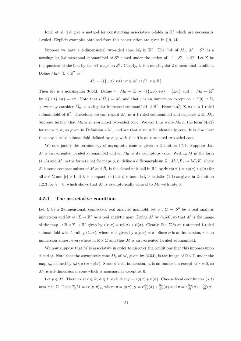
Ionel et al. [19] give a method for constructing associative 3-folds in R7 which are necessarily
1-ruled. Explicit examples obtained from this construction are given in [19, §4].
Suppose we have a 3-dimensional two-sided cone M0 in R7. The link of M0, M0 ∩ S6, is a
nonsingular 2-dimensional submanifold of S6 closed under the action of −1 : S6 → S6. Let Σ be
the quotient of the link by the ±1 maps on S6. Clearly, Σ is a nonsingular 2-dimensional manifold.
Define M0 ⊆ Σ× R7 by:
M0 = (±σ, rσ) : σ ∈ M0 ∩ S6, r ∈ R.
Then M0 is a nonsingular 3-fold. Define π : M0 → Σ by π(±σ, rσ) = ±σ and ι : M0 → R7
by ι(±σ, rσ) = rσ. Note that ι(M0) = M0 and that ι is an immersion except on ι−1(0) ∼= Σ,
so we may consider M0 as a singular immersed submanifold of R7. Hence (M0,Σ, π) is a 1-ruled
submanifold of R7. Therefore, we can regard M0 as a 1-ruled submanifold and dispense with M0.
Suppose further that M0 is an r-oriented two-sided cone. We can thus write M0 in the form (4.53)
for maps φ, ψ, as given in Definition 4.5.1, and see that ψ must be identically zero. It is also clear
that any 1-ruled submanifold defined by φ, ψ with ψ ≡ 0 is an r-oriented two-sided cone.
We now justify the terminology of asymptotic cone as given in Definition 4.5.1. Suppose that
M is an r-oriented 1-ruled submanifold and let M0 be its asymptotic cone. Writing M in the form
(4.53) and M0 in the form (4.54) for maps φ, ψ, define a diffeomorphism Ψ : M0\B1 → M \K, where
K is some compact subset of M and B1 is the closed unit ball in R7, by Ψ(rφ(σ)) = rφ(σ)+ψ(σ) for
all σ ∈ Σ and |r| > 1. If Σ is compact, so that ψ is bounded, Ψ satisfies (1.1) as given in Definition
1.2.3 for λ = 0, which shows that M is asymptotically conical to M0 with rate 0.
4.5.1 The associative condition
Let Σ be a 2-dimensional, connected, real analytic manifold, let φ : Σ → S6 be a real analytic
immersion and let ψ : Σ → R7 be a real analytic map. Define M by (4.53), so that M is the image
of the map ι : R× Σ → R7 given by ι(r, σ) = rφ(σ) + ψ(σ). Clearly, R× Σ is an r-oriented 1-ruled
submanifold with 1-ruling (Σ, π), where π is given by π(r, σ) = σ. Since φ is an immersion, ι is an
immersion almost everywhere in R× Σ and thus M is an r-oriented 1-ruled submanifold.
We now suppose that M is associative in order to discover the conditions that this imposes upon
φ and ψ. Note that the asymptotic cone M0 of M , given by (4.54), is the image of R×Σ under the
map ι0, defined by ι0(r, σ) = rφ(σ). Since φ is an immersion, ι0 is an immersion except at r = 0, so
M0 is a 3-dimensional cone which is nonsingular except at 0.
Let p ∈ M . There exist r ∈ R, σ ∈ Σ such that p = rφ(σ)+ψ(σ). Choose local coordinates (s, t)
near σ in Σ. Then TpM = 〈x,y, z〉R, where x = φ(σ), y = r ∂φ∂s (σ)+ ∂ψ
∂s (σ) and z = r ∂φ∂t (σ)+ ∂ψ
∂t (σ).
51
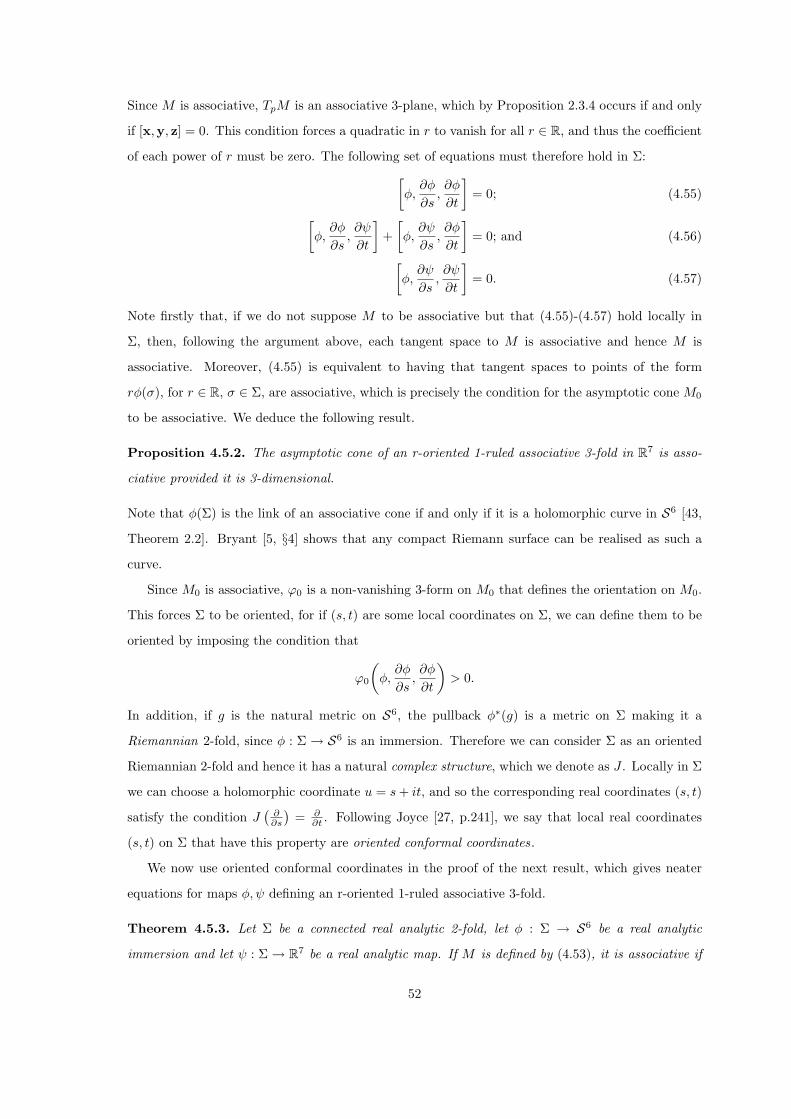
Since M is associative, TpM is an associative 3-plane, which by Proposition 2.3.4 occurs if and only
if [x,y, z] = 0. This condition forces a quadratic in r to vanish for all r ∈ R, and thus the coefficient
of each power of r must be zero. The following set of equations must therefore hold in Σ:[φ,
∂φ
∂s,∂φ
∂t
]= 0; (4.55)
[φ,
∂φ
∂s,∂ψ
∂t
]+
[φ,
∂ψ
∂s,∂φ
∂t
]= 0; and (4.56)
[φ,
∂ψ
∂s,∂ψ
∂t
]= 0. (4.57)
Note firstly that, if we do not suppose M to be associative but that (4.55)-(4.57) hold locally in
Σ, then, following the argument above, each tangent space to M is associative and hence M is
associative. Moreover, (4.55) is equivalent to having that tangent spaces to points of the form
rφ(σ), for r ∈ R, σ ∈ Σ, are associative, which is precisely the condition for the asymptotic cone M0
to be associative. We deduce the following result.
Proposition 4.5.2. The asymptotic cone of an r-oriented 1-ruled associative 3-fold in R7 is asso-
ciative provided it is 3-dimensional.
Note that φ(Σ) is the link of an associative cone if and only if it is a holomorphic curve in S6 [43,
Theorem 2.2]. Bryant [5, §4] shows that any compact Riemann surface can be realised as such a
curve.
Since M0 is associative, ϕ0 is a non-vanishing 3-form on M0 that defines the orientation on M0.
This forces Σ to be oriented, for if (s, t) are some local coordinates on Σ, we can define them to be
oriented by imposing the condition that
ϕ0
(φ,
∂φ
∂s,∂φ
∂t
)> 0.
In addition, if g is the natural metric on S6, the pullback φ∗(g) is a metric on Σ making it a
Riemannian 2-fold, since φ : Σ → S6 is an immersion. Therefore we can consider Σ as an oriented
Riemannian 2-fold and hence it has a natural complex structure, which we denote as J . Locally in Σ
we can choose a holomorphic coordinate u = s + it, and so the corresponding real coordinates (s, t)
satisfy the condition J(
∂∂s
)= ∂
∂t . Following Joyce [27, p.241], we say that local real coordinates
(s, t) on Σ that have this property are oriented conformal coordinates.
We now use oriented conformal coordinates in the proof of the next result, which gives neater
equations for maps φ, ψ defining an r-oriented 1-ruled associative 3-fold.
Theorem 4.5.3. Let Σ be a connected real analytic 2-fold, let φ : Σ → S6 be a real analytic
immersion and let ψ : Σ → R7 be a real analytic map. If M is defined by (4.53), it is associative if
52

and only if∂φ
∂t= φ× ∂φ
∂s(4.58)
and ψ satisfies
(i)∂ψ
∂t= φ× ∂ψ
∂s+ fφ for some real analytic function f : Σ → R,
or
(ii)∂ψ
∂s(σ),
∂ψ
∂t(σ) ∈
⟨φ(σ),
∂φ
∂s(σ),
∂φ
∂t(σ)
⟩
Rfor all σ ∈ Σ,
where × is defined by (2.9) and (s, t) are oriented conformal coordinates on Σ.
Proof. Above we noted that (4.55)-(4.57) were equivalent to the condition that M is associative, so
we show that (4.58) is equivalent to (4.55) and that (i) and (ii) are equivalent to (4.56) and (4.57).
Let σ ∈ Σ, C = |∂φ∂s (σ)| > 0. Since φ maps to the unit sphere in R7, φ(σ) is orthogonal to
∂φ∂s (σ) and ∂φ
∂t (σ). As (s, t) are oriented conformal coordinates, we also see that ∂φ∂s (σ) and ∂φ
∂t (σ)
are orthogonal and that |∂φ∂t (σ)| = C. We conclude that the triple (φ(σ), C−1 ∂φ
∂s (σ), C−1 ∂φ∂t (σ)) is
an oriented orthonormal triad in R7, and it is the basis for an associative 3-plane in R7 if and only if
(4.55) holds at σ. Since G2 acts transitively on the set of associative 3-planes [17, Theorem IV.1.8],
if (4.55) holds at σ we can transform coordinates on R7 using G2 so that
φ(σ) = e1,∂φ
∂s(σ) = Ce2 and
∂φ
∂t(σ) = Ce3,
where e1, . . . , e7 is a basis for ImO ∼= R7. We note here that (4.58) holds at σ since the cross
product is invariant under G2 by Definition 2.1.8. If (4.58) holds at σ, the 3-plane generated by
φ(σ), ∂φ∂s (σ), ∂φ
∂t (σ) is associative by Corollary 2.3.5.
Under the change of coordinates of R7 above, we can write ∂ψ∂s (σ) = a1e1 + . . . + a7e7 and
∂ψ∂t (σ) = b1e1 + . . . + b7e7 for real constants aj , bj for j = 1, . . . , 7. Calculations show that (4.56)
holds at σ if and only if
b4 = −a5, b5 = a4, b6 = −a7, b7 = a6, (4.59)
and (4.57) holds at σ if and only if
−a4b7 − a5b6 + a6b5 + b4a7 = 0, −a4b6 + a5b7 + a6b4 − a7b5 = 0, (4.60)
a2b7 + a3b6 − a6b3 − a7b2 = 0, a2b6 − a3b7 − a6b2 + a7b3 = 0, (4.61)
−a2b5 − a3b4 + a4b3 + a5b2 = 0 and −a2b4 + a3b5 + a4b2 − a5b3 = 0. (4.62)
53
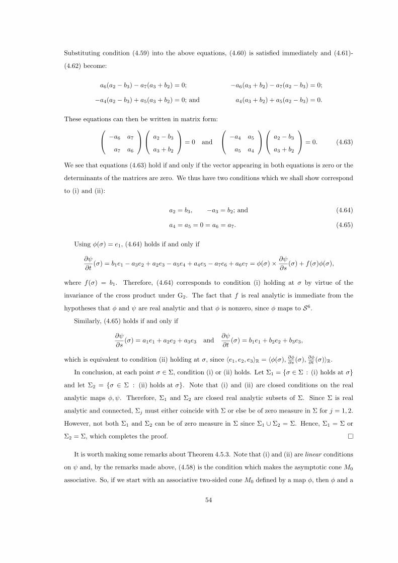
Substituting condition (4.59) into the above equations, (4.60) is satisfied immediately and (4.61)-
(4.62) become:
a6(a2 − b3)− a7(a3 + b2) = 0; −a6(a3 + b2)− a7(a2 − b3) = 0;
−a4(a2 − b3) + a5(a3 + b2) = 0; and a4(a3 + b2) + a5(a2 − b3) = 0.
These equations can then be written in matrix form: −a6 a7
a7 a6
a2 − b3
a3 + b2
= 0 and
−a4 a5
a5 a4
a2 − b3
a3 + b2
= 0. (4.63)
We see that equations (4.63) hold if and only if the vector appearing in both equations is zero or the
determinants of the matrices are zero. We thus have two conditions which we shall show correspond
to (i) and (ii):
a2 = b3, −a3 = b2; and (4.64)
a4 = a5 = 0 = a6 = a7. (4.65)
Using φ(σ) = e1, (4.64) holds if and only if
∂ψ
∂t(σ) = b1e1 − a3e2 + a2e3 − a5e4 + a4e5 − a7e6 + a6e7 = φ(σ)× ∂ψ
∂s(σ) + f(σ)φ(σ),
where f(σ) = b1. Therefore, (4.64) corresponds to condition (i) holding at σ by virtue of the
invariance of the cross product under G2. The fact that f is real analytic is immediate from the
hypotheses that φ and ψ are real analytic and that φ is nonzero, since φ maps to S6.
Similarly, (4.65) holds if and only if
∂ψ
∂s(σ) = a1e1 + a2e2 + a3e3 and
∂ψ
∂t(σ) = b1e1 + b2e2 + b3e3,
which is equivalent to condition (ii) holding at σ, since 〈e1, e2, e3〉R = 〈φ(σ), ∂φ∂s (σ), ∂φ
∂t (σ)〉R.In conclusion, at each point σ ∈ Σ, condition (i) or (ii) holds. Let Σ1 = σ ∈ Σ : (i) holds at σ
and let Σ2 = σ ∈ Σ : (ii) holds at σ. Note that (i) and (ii) are closed conditions on the real
analytic maps φ, ψ. Therefore, Σ1 and Σ2 are closed real analytic subsets of Σ. Since Σ is real
analytic and connected, Σj must either coincide with Σ or else be of zero measure in Σ for j = 1, 2.
However, not both Σ1 and Σ2 can be of zero measure in Σ since Σ1 ∪ Σ2 = Σ. Hence, Σ1 = Σ or
Σ2 = Σ, which completes the proof.
It is worth making some remarks about Theorem 4.5.3. Note that (i) and (ii) are linear conditions
on ψ and, by the remarks made above, (4.58) is the condition which makes the asymptotic cone M0
associative. So, if we start with an associative two-sided cone M0 defined by a map φ, then φ and a
54

function ψ satisfying (i) or (ii) will define an r-oriented 1-ruled associative 3-fold M with asymptotic
cone M0. We also note that conditions (i) and (ii) are unchanged if φ is fixed and satisfies (4.58), but
ψ is replaced by ψ + fφ where f is a real analytic function. We can thus always locally transform
ψ such that f in condition (i) is zero, if we relax the condition that ψ is orthogonal to φ.
4.5.2 The partial differential equations
Our first result follows [27, Proposition 5.2]. We make the definition that a function is real analytic
on a compact interval I in R if it extends to a real analytic function on an open set containing I.
Theorem 4.5.4. Let I be a compact interval in R, let s be a coordinate on I and let φ0 : I → S6 and
ψ0 : I → R7 be real analytic maps. There exist ε > 0 and unique real analytic maps φ : I× (−ε, ε) →S6 and ψ : I × (−ε, ε) → R7 satisfying φ(s, 0) = φ0(s), ψ(s, 0) = ψ0(s) for all s ∈ I, and
∂φ
∂t= φ× ∂φ
∂sand
∂ψ
∂t= φ× ∂ψ
∂s, (4.66)
where t is a coordinate on (−ε, ε) and × is defined in (2.9). If M is given by
M = rφ(s, t) + ψ(s, t) : r ∈ R, s ∈ I, t ∈ (−ε, ε),
it is an r-oriented 1-ruled associative 3-fold in R7.
Proof. Since I is compact and φ0, ψ0 are real analytic, we may use the Cauchy–Kowalevsky Theorem
(Theorem 1.1.4) to give us functions φ : I × (−ε, ε) → R7 and ψ : I × (−ε, ε) → R7 satisfying the
initial conditions and (4.66). It is clear that ∂∂t g(φ, φ) = 2g(φ, ∂φ
∂t ) = 0, since ∂φ∂t is defined by a cross
product involving φ and hence is orthogonal to φ by (2.8). We deduce that |φ| is independent of t
and is therefore one, so that φ maps to S6. We conclude that M is an r-oriented 1-ruled associative
3-fold using (i) of Theorem 4.5.3.
Theorem 4.5.4 shows that (4.66) can be considered as evolution equations for maps φ and ψ satisfying
(i) of Theorem 4.5.3. We now show that condition (ii) of Theorem 4.5.3 does not produce any
interesting 1-ruled associative 3-folds. We say that two 1-rulings (Σ, π) and (Σ, π) are distinct if the
families of affine straight lines FΣ = π−1(σ) : σ ∈ Σ and FΣ = π−1(σ) : σ ∈ Σ are different.
Proposition 4.5.5. Any r-oriented 1-ruled associative 3-fold (M, Σ, π) satisfying condition (ii) but
not (i) of Theorem 4.5.3 is locally isomorphic to an affine associative 3-plane in R7.
Proof. By Theorem 4.1.1, M is real analytic wherever it is nonsingular and so we can take (Σ, π) to
be locally real analytic. Let I = [0, 1], let γ : I → Σ be a real analytic curve in Σ and let φ, ψ be
the functions defining M . Then we can use Theorem 4.5.4 with initial conditions φ0 = φ(γ(s)) and
55

ψ0 = ψ(γ(s)) to give us functions φ and ψ which define an r-oriented 1-ruled associative 3-fold M
satisfying (i) of Theorem 4.5.3. However, M and M coincide in the real analytic 2-fold π−1(γ(I)),
and hence, by Theorem 4.1.2, they must be locally equal. We conclude that M locally admits a
1-ruling (Σ, π) satisfying (i) of Theorem 4.5.3, which must therefore be distinct from (Σ, π).
The families of affine straight lines FΣ and FΣ, using the notation above, coincide in the family
of affine straight lines defined by points on γ, denoted Fγ . Using local real analyticity of the families,
either FΣ is equal to FΣ locally or they only meet in Fγ locally. The former possibility is excluded
because the 1-rulings (Σ, π) and (Σ, π) are distinct and thus the latter is true.
Let γ1 and γ2 be distinct real analytic curves near γ in Σ defining 1-rulings (Σ1, π1) and (Σ2, π2),
respectively, as above. Then FΣ ∩ FΣjis locally equal to Fγj
for j = 1, 2. Hence, (Σ1, π1) and
(Σ2, π2) are not distinct (that is, FΣ1 = FΣ2) if and only if Fγ1 = Fγ2 , which implies that γ1 = γ2.
Therefore, distinct curves near γ in Σ produce different 1-rulings of M and thus M has infinitely
many 1-rulings.
Suppose that γt : t ∈ R is a one parameter family of distinct curves near γ in Σ, with γ0 = γ.
Each curve in the family defines a distinct 1-ruling (Σt, πt), hence there exists p ∈ M with M
nonsingular at p such that Lt = π−1t (πt(p)) is not constant as a line in R7. We therefore get a one
parameter family of lines Lt in M through p with dLt
dt 6= 0 at some point, i.e. such that Lt changes
nontrivially. We have thus constructed a real analytic one-dimensional family of lines Lt : t ∈ Rwhose total space is a real analytic 2-fold N contained in M . Moreover, every line in M through p
is a line in the affine associative 3-plane p + TpM , so N is contained in p + TpM . Then, since N
has nonsingular points in the intersection between M and p + TpM , Theorem 4.1.2 shows that M
and p + TpM coincide on a component of M . Hence, M is planar, i.e. M is locally isomorphic to
an affine associative 3-plane in R7.
In the course of the proof above, we have shown that a 1-ruled associative 3-fold which admits a
one parameter family of distinct real analytic 1-rulings is planar. This is analogous to the result [7,
Theorem 6 part 2], which relates to 1-ruled SL 3-folds.
We combine our results on 1-ruled associative 3-folds into the following theorem.
Theorem 4.5.6. Let (M, Σ, π) be a non-planar, r-oriented, 1-ruled associative 3-fold in R7. There
exist real analytic maps φ : Σ → S6 and ψ : Σ → R7 such that:
M = rφ(σ) + ψ(σ) : r ∈ R, σ ∈ Σ ;
∂φ
∂t= φ× ∂φ
∂s; and (4.67)
∂ψ
∂t= φ× ∂ψ
∂s+ fφ , (4.68)
56
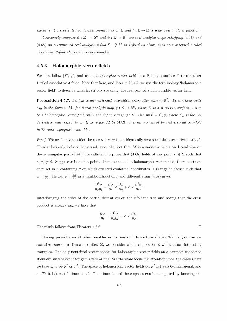
where (s, t) are oriented conformal coordinates on Σ and f : Σ → R is some real analytic function.
Conversely, suppose φ : Σ → S6 and ψ : Σ → R7 are real analytic maps satisfying (4.67) and
(4.68) on a connected real analytic 2-fold Σ. If M is defined as above, it is an r-oriented 1-ruled
associative 3-fold wherever it is nonsingular.
4.5.3 Holomorphic vector fields
We now follow [27, §6] and use a holomorphic vector field on a Riemann surface Σ to construct
1-ruled associative 3-folds. Note that here, and later in §5.4.5, we use the terminology ‘holomorphic
vector field’ to describe what is, strictly speaking, the real part of a holomorphic vector field.
Proposition 4.5.7. Let M0 be an r-oriented, two-sided, associative cone in R7. We can then write
M0 in the form (4.54) for a real analytic map φ : Σ → S6, where Σ is a Riemann surface. Let w
be a holomorphic vector field on Σ and define a map ψ : Σ → R7 by ψ = Lwφ, where Lw is the Lie
derivative with respect to w. If we define M by (4.53), it is an r-oriented 1-ruled associative 3-fold
in R7 with asymptotic cone M0.
Proof. We need only consider the case where w is not identically zero since the alternative is trivial.
Then w has only isolated zeros and, since the fact that M is associative is a closed condition on
the nonsingular part of M , it is sufficient to prove that (4.68) holds at any point σ ∈ Σ such that
w(σ) 6= 0. Suppose σ is such a point. Then, since w is a holomorphic vector field, there exists an
open set in Σ containing σ on which oriented conformal coordinates (s, t) may be chosen such that
w = ∂∂s . Hence, ψ = ∂φ
∂s in a neighbourhood of σ and differentiating (4.67) gives:
∂2φ
∂s∂t=
∂φ
∂s× ∂φ
∂s+ φ× ∂2φ
∂s2.
Interchanging the order of the partial derivatives on the left-hand side and noting that the cross
product is alternating, we have that
∂ψ
∂t=
∂2φ
∂s∂t= φ× ∂ψ
∂s.
The result follows from Theorem 4.5.6.
Having proved a result which enables us to construct 1-ruled associative 3-folds given an as-
sociative cone on a Riemann surface Σ, we consider which choices for Σ will produce interesting
examples. The only nontrivial vector spaces for holomorphic vector fields on a compact connected
Riemann surface occur for genus zero or one. We therefore focus our attention upon the cases where
we take Σ to be S2 or T 2. The space of holomorphic vector fields on S2 is (real) 6-dimensional, and
on T 2 it is (real) 2-dimensional. The dimension of these spaces can be computed by knowing the
57
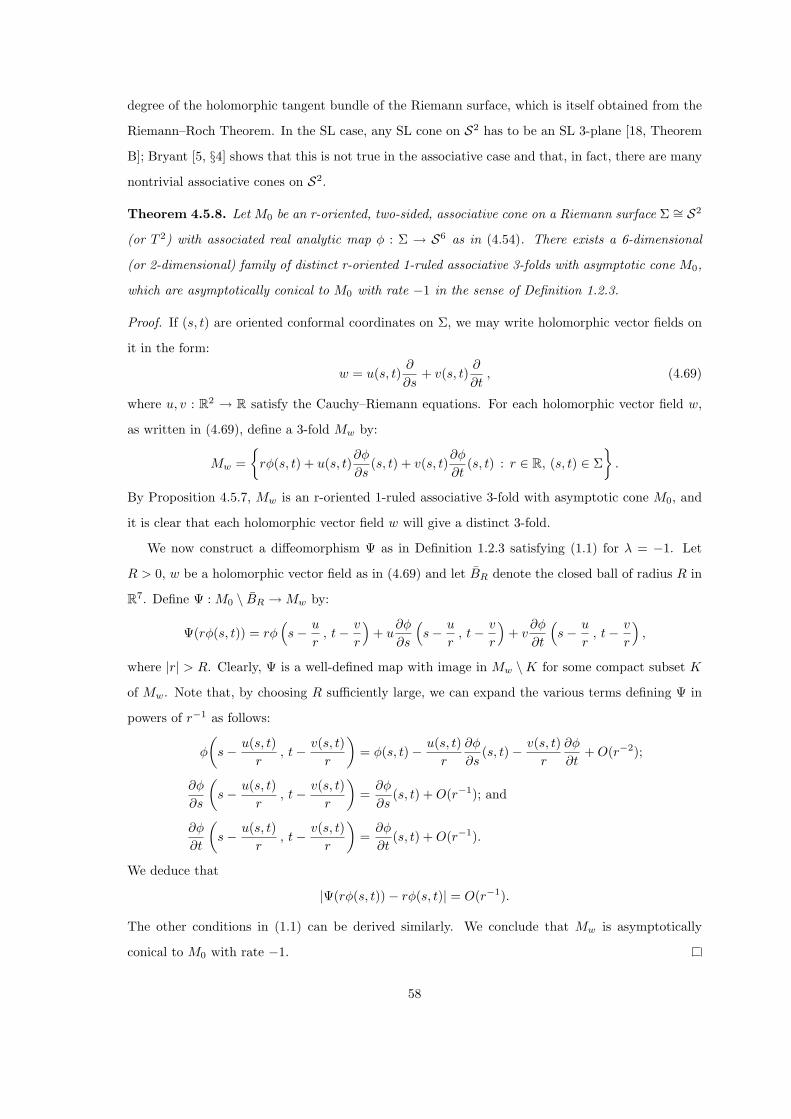
degree of the holomorphic tangent bundle of the Riemann surface, which is itself obtained from the
Riemann–Roch Theorem. In the SL case, any SL cone on S2 has to be an SL 3-plane [18, Theorem
B]; Bryant [5, §4] shows that this is not true in the associative case and that, in fact, there are many
nontrivial associative cones on S2.
Theorem 4.5.8. Let M0 be an r-oriented, two-sided, associative cone on a Riemann surface Σ ∼= S2
(or T 2) with associated real analytic map φ : Σ → S6 as in (4.54). There exists a 6-dimensional
(or 2-dimensional) family of distinct r-oriented 1-ruled associative 3-folds with asymptotic cone M0,
which are asymptotically conical to M0 with rate −1 in the sense of Definition 1.2.3.
Proof. If (s, t) are oriented conformal coordinates on Σ, we may write holomorphic vector fields on
it in the form:
w = u(s, t)∂
∂s+ v(s, t)
∂
∂t, (4.69)
where u, v : R2 → R satisfy the Cauchy–Riemann equations. For each holomorphic vector field w,
as written in (4.69), define a 3-fold Mw by:
Mw =
rφ(s, t) + u(s, t)∂φ
∂s(s, t) + v(s, t)
∂φ
∂t(s, t) : r ∈ R, (s, t) ∈ Σ
.
By Proposition 4.5.7, Mw is an r-oriented 1-ruled associative 3-fold with asymptotic cone M0, and
it is clear that each holomorphic vector field w will give a distinct 3-fold.
We now construct a diffeomorphism Ψ as in Definition 1.2.3 satisfying (1.1) for λ = −1. Let
R > 0, w be a holomorphic vector field as in (4.69) and let BR denote the closed ball of radius R in
R7. Define Ψ : M0 \ BR → Mw by:
Ψ(rφ(s, t)) = rφ(s− u
r, t− v
r
)+ u
∂φ
∂s
(s− u
r, t− v
r
)+ v
∂φ
∂t
(s− u
r, t− v
r
),
where |r| > R. Clearly, Ψ is a well-defined map with image in Mw \K for some compact subset K
of Mw. Note that, by choosing R sufficiently large, we can expand the various terms defining Ψ in
powers of r−1 as follows:
φ
(s− u(s, t)
r, t− v(s, t)
r
)= φ(s, t)− u(s, t)
r
∂φ
∂s(s, t)− v(s, t)
r
∂φ
∂t+ O(r−2);
∂φ
∂s
(s− u(s, t)
r, t− v(s, t)
r
)=
∂φ
∂s(s, t) + O(r−1); and
∂φ
∂t
(s− u(s, t)
r, t− v(s, t)
r
)=
∂φ
∂t(s, t) + O(r−1).
We deduce that
|Ψ(rφ(s, t))− rφ(s, t)| = O(r−1).
The other conditions in (1.1) can be derived similarly. We conclude that Mw is asymptotically
conical to M0 with rate −1.
58

4.5.4 Examples
There are many examples of associative cones over T 2 given by the SL tori constructed by Haskins
[18], Joyce [24], McIntosh [44] and others. However, by Theorem 4.4.7, applying Theorem 4.5.8 to
them will only produce 1-ruled SL 3-folds and the result reduces to [27, Theorem 6.3]. However, we
also have the associative cones over T 2 given by Theorem 4.2.6. This family of cones is determined by
four real parameters, whereas the corresponding SL family, as discussed in [24, §7], is parameterised
by one rational variable. Therefore, these cones are generically not SL and so we get the following
examples of 1-ruled associative 3-folds.
Theorem 4.5.9. Use the notation of Theorem 4.2.4 and suppose that α2 = α3 = −1. Let M ,
as given in Theorem 4.2.4, be an associative cone over T 2, which, by Theorem 4.2.6, occurs for
generic choices of x1(0), z1(0), z2(0) and z3(0). Let u, v : R2 → R be functions satisfying the
Cauchy–Riemann equations and let M0 = M ∪ (−M) ∪ 0. The subset Mu,v of R⊕ C3 given by
Mu,v =(
rx1(t) + v(s, t)(2|z1(t)|2 − |z2(t)|2 − |z3(t)|2
), e2is
(r + 2iu(s, t)− 2v(s, t)x1(t)
)z1(t),
e−is((
r − iu(s, t) + v(s, t)x1(t))z2(t)− 3iv(s, t)z3z1
),
e−is((
r − iu(s, t) + v(s, t)x1(t))z3(t) + 3iv(s, t)z1z2
)): r, s, t ∈ R
is an r-oriented 1-ruled associative 3-fold in R7 ∼= R⊕C3. Moreover, Mu,v is asymptotically conical
to M0 with rate −1 in the sense of Definition 1.2.3.
Proof. Define φ : R2 → R⊕ C3 ∼= R7 by
φ(s, t) = (x1(t), e2isz1(t), e−isz2(t), e−isz3(t)).
Since x21 + |z1|2 + |z2|2 + |z3|2 = 1, φ maps into S6 and we can write M0 in the form (4.54). Define
a holomorphic vector field w using u and v as in (4.69). Applying Proposition 4.5.7 and using
equations (4.21)-(4.24) of Theorem 4.2.4 gives Mu,v as stated. Since M0 is a cone over T 2, Theorem
4.5.8 gives us the final line.
Note that, although M and hence M0 is U(1)-invariant, Mu,v will not be in general.
59

Chapter 5
Coassociative 4-folds in R7 and
Cayley 4-folds in R8
The focus of this chapter is on constructing examples of coassociative and Cayley 4-folds in R7 and
R8 respectively. Our examples can be split into two categories. The first set, described in Sections
5.2 and 5.3, comprises 4-folds with symmetries which are constructed using evolution equations. The
second consists of 2-ruled submanifolds and forms the content of Section 5.4. The motivation for
our study comes from [24], [27] and the work in the previous chapter.
5.1 Evolution Equations
To derive evolution equations for coassociative and Cayley 4-folds we need some results related to
real analyticity. The first is an obvious corollary of Theorem 1.1.3.
Theorem 5.1.1. A coassociative 4-fold in R7 or a Cayley 4-fold in R8 is real analytic wherever it
is nonsingular.
The next two results, [17, Theorem IV.4.3] and [17, Theorem IV.4.6], use real analyticity since their
proofs rely upon the Cartan–Kahler Theorem, which is only applicable in the real analytic category.
Theorem 5.1.2. Suppose P is a 3-dimensional real analytic submanifold of ImO ∼= R7 such that
ϕ0|P ≡ 0. There locally exists a real analytic coassociative 4-fold N in R7 which contains P .
Moreover, N is locally unique.
Notice here that, unlike Theorem 4.1.2 for associative 3-folds in R7, we have to impose an extra
condition on the boundary submanifold P in order to extend it to a coassociative 4-fold in R7.
60
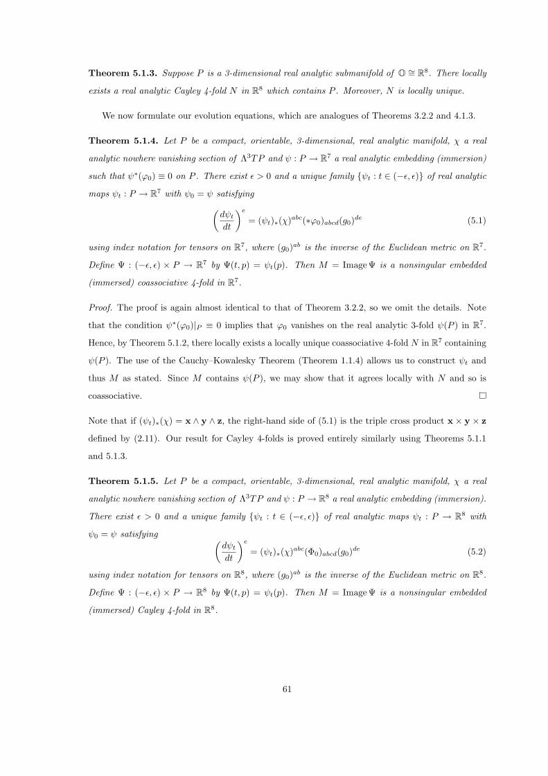
Theorem 5.1.3. Suppose P is a 3-dimensional real analytic submanifold of O ∼= R8. There locally
exists a real analytic Cayley 4-fold N in R8 which contains P . Moreover, N is locally unique.
We now formulate our evolution equations, which are analogues of Theorems 3.2.2 and 4.1.3.
Theorem 5.1.4. Let P be a compact, orientable, 3-dimensional, real analytic manifold, χ a real
analytic nowhere vanishing section of Λ3TP and ψ : P → R7 a real analytic embedding (immersion)
such that ψ∗(ϕ0) ≡ 0 on P . There exist ε > 0 and a unique family ψt : t ∈ (−ε, ε) of real analytic
maps ψt : P → R7 with ψ0 = ψ satisfying(
dψt
dt
)e
= (ψt)∗(χ)abc(∗ϕ0)abcd(g0)de (5.1)
using index notation for tensors on R7, where (g0)ab is the inverse of the Euclidean metric on R7.
Define Ψ : (−ε, ε) × P → R7 by Ψ(t, p) = ψt(p). Then M = Image Ψ is a nonsingular embedded
(immersed) coassociative 4-fold in R7.
Proof. The proof is again almost identical to that of Theorem 3.2.2, so we omit the details. Note
that the condition ψ∗(ϕ0)|P ≡ 0 implies that ϕ0 vanishes on the real analytic 3-fold ψ(P ) in R7.
Hence, by Theorem 5.1.2, there locally exists a locally unique coassociative 4-fold N in R7 containing
ψ(P ). The use of the Cauchy–Kowalesky Theorem (Theorem 1.1.4) allows us to construct ψt and
thus M as stated. Since M contains ψ(P ), we may show that it agrees locally with N and so is
coassociative.
Note that if (ψt)∗(χ) = x ∧ y ∧ z, the right-hand side of (5.1) is the triple cross product x× y × z
defined by (2.11). Our result for Cayley 4-folds is proved entirely similarly using Theorems 5.1.1
and 5.1.3.
Theorem 5.1.5. Let P be a compact, orientable, 3-dimensional, real analytic manifold, χ a real
analytic nowhere vanishing section of Λ3TP and ψ : P → R8 a real analytic embedding (immersion).
There exist ε > 0 and a unique family ψt : t ∈ (−ε, ε) of real analytic maps ψt : P → R8 with
ψ0 = ψ satisfying (dψt
dt
)e
= (ψt)∗(χ)abc(Φ0)abcd(g0)de (5.2)
using index notation for tensors on R8, where (g0)ab is the inverse of the Euclidean metric on R8.
Define Ψ : (−ε, ε) × P → R8 by Ψ(t, p) = ψt(p). Then M = Image Ψ is a nonsingular embedded
(immersed) Cayley 4-fold in R8.
61
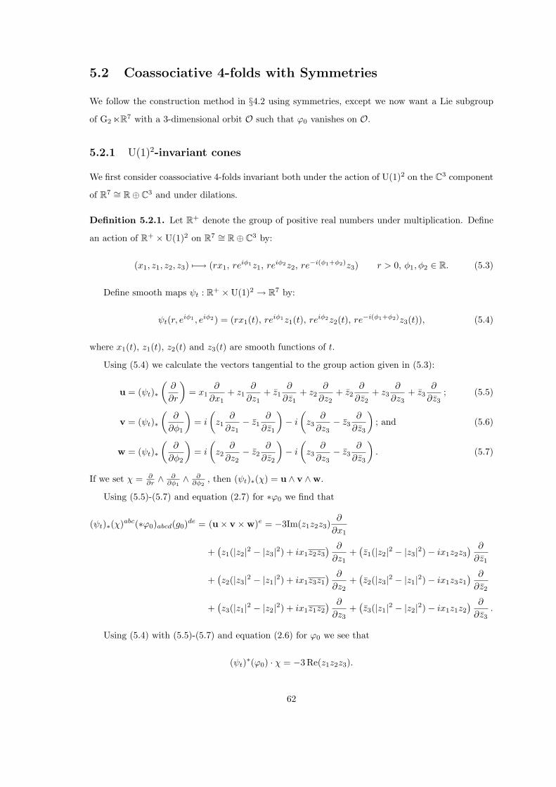
5.2 Coassociative 4-folds with Symmetries
We follow the construction method in §4.2 using symmetries, except we now want a Lie subgroup
of G2nR7 with a 3-dimensional orbit O such that ϕ0 vanishes on O.
5.2.1 U(1)2-invariant cones
We first consider coassociative 4-folds invariant both under the action of U(1)2 on the C3 component
of R7 ∼= R⊕ C3 and under dilations.
Definition 5.2.1. Let R+ denote the group of positive real numbers under multiplication. Define
an action of R+ ×U(1)2 on R7 ∼= R⊕ C3 by:
(x1, z1, z2, z3) 7−→ (rx1, reiφ1z1, reiφ2z2, re−i(φ1+φ2)z3) r > 0, φ1, φ2 ∈ R. (5.3)
Define smooth maps ψt : R+ ×U(1)2 → R7 by:
ψt(r, eiφ1 , eiφ2) = (rx1(t), reiφ1z1(t), reiφ2z2(t), re−i(φ1+φ2)z3(t)), (5.4)
where x1(t), z1(t), z2(t) and z3(t) are smooth functions of t.
Using (5.4) we calculate the vectors tangential to the group action given in (5.3):
u = (ψt)∗
(∂
∂r
)= x1
∂
∂x1+ z1
∂
∂z1+ z1
∂
∂z1+ z2
∂
∂z2+ z2
∂
∂z2+ z3
∂
∂z3+ z3
∂
∂z3; (5.5)
v = (ψt)∗
(∂
∂φ1
)= i
(z1
∂
∂z1− z1
∂
∂z1
)− i
(z3
∂
∂z3− z3
∂
∂z3
); and (5.6)
w = (ψt)∗
(∂
∂φ2
)= i
(z2
∂
∂z2− z2
∂
∂z2
)− i
(z3
∂
∂z3− z3
∂
∂z3
). (5.7)
If we set χ = ∂∂r ∧ ∂
∂φ1∧ ∂
∂φ2, then (ψt)∗(χ) = u ∧ v ∧w.
Using (5.5)-(5.7) and equation (2.7) for ∗ϕ0 we find that
(ψt)∗(χ)abc(∗ϕ0)abcd(g0)de = (u× v ×w)e = −3Im(z1z2z3)∂
∂x1
+(z1(|z2|2 − |z3|2) + ix1z2z3
) ∂
∂z1+
(z1(|z2|2 − |z3|2)− ix1z2z3
) ∂
∂z1
+(z2(|z3|2 − |z1|2) + ix1z3z1
) ∂
∂z2+
(z2(|z3|2 − |z1|2)− ix1z3z1
) ∂
∂z2
+(z3(|z1|2 − |z2|2) + ix1z1z2
) ∂
∂z3+
(z3(|z1|2 − |z2|2)− ix1z1z2
) ∂
∂z3.
Using (5.4) with (5.5)-(5.7) and equation (2.6) for ϕ0 we see that
(ψt)∗(ϕ0) · χ = −3Re(z1z2z3).
62

Therefore (ψt)∗(ϕ0) ≡ 0 is equivalent to Re(z1z2z3) = 0.
We also see thatdψt
dt=
dx1
dt
∂
∂x1+
3∑
j=1
dzj
dt
∂
∂zj+
3∑
j=1
dzj
dt
∂
∂zj.
We then deduce our result from Theorem 5.1.4.
Theorem 5.2.2. Let x1 : R→ R and z1, z2, z3 : R→ C be differentiable functions satisfying
dx1
dt= −3Im(z1z2z3), (5.8)
dz1
dt= z1(|z2|2 − |z3|2) + ix1z2z3, (5.9)
dz2
dt= z2(|z3|2 − |z1|2) + ix1z3z1 and (5.10)
dz3
dt= z3(|z1|2 − |z2|2) + ix1z1z2, (5.11)
along with the condition
Re(z1z2z3) = 0 (5.12)
at t = 0. The subset M of R⊕ C3 ∼= R7 defined by
M =
(rx1(t), reiφ1z1(t), reiφ2z2(t), re−i(φ1+φ2)z3(t)) : r > 0, φ1, φ2, t ∈ R
is a coassociative 4-fold in R7. Moreover, (5.12) holds for all t ∈ R and x21 + |z1|2 + |z2|2 + |z3|2 is
a constant which can be taken to be 1.
Proof. It is immediate from (5.8)-(5.11) that x21 + |z1|2 + |z2|2 + |z3|2 is a constant which can be
chosen to be 1 without loss of generality. We may also calculate
d
dt(z1z2z3) = ix1(|z2|2|z3|2 + |z3|2|z1|2 + |z1|2|z2|2)
using (5.8)-(5.11) and deduce that Re(z1z2z3) is a constant which has to be zero since (5.12) holds
at t = 0. Theorem 5.1.4 only gives us that solutions to (5.8)-(5.11) exist for t ∈ (−ε, ε) for some
ε > 0, but it is possible, as in §4.2.2, to show that solutions exist for all t as the functions involved
are all bounded.
5.2.2 SU(2) symmetry 1
There are three different natural actions of SU(2) on R7 in G2. The first is where SU(2) acts on
R7 ∼= R3 ⊕ C2 with the standard SU(2) action on C2 and trivially on R3. The construction using
this action produces an affine C2 ⊆ R7 as the coassociative 4-fold. The second has SU(2) acting on
63

R7 ∼= R⊕C3 as SO(3) on C3 and trivially on R. The construction then produces a complex surface
in R7 as the coassociative 4-fold, which we may be written as follows:
(x1, z1, z2, z3) : z2
1 + z22 + z2
3 = A, x1 = B
, where A ∈ C and B ∈ R are constants.
The final action on R7 ∼= R3 ⊕ C2, where the isomorphism R4 ∼= C2 is given by (x4, x5, x6, x7) 7→(x4 + ix6, x5 + ix7), has an SU(2) action on C2 and an action of SO(3) = SU(2)/±1 on R3.
Harvey and Lawson [17, IV.3] have already studied coassociative 4-folds invariant under this action
by different means.
Definition 5.2.3. Let X ∈ SU(2) and let (x1, x2, x3, z1, z2) ∈ R3⊕C2 ∼= R7 with z1 = x4 + ix6 and
z2 = x5 + ix7. There exist a, b ∈ C such that |a|2 + |b|2 = 1 and
X =
a b
−b a
.
We define the action of X on (x1, x2, x3, z1, z2) by:
x1
x2
x3
7−→
|a|2 − |b|2 2Re(ab) −2Im(ab)
−2Re(ab) Re(a2 − b2) −Im(a2 − b2)
−2Im(ab) Im(a2 + b2) Re(a2 + b2)
x1
x2
x3
z1
z2
7−→
a b
−b a
z1
z2
.
Denote this action by X · (x1, x2, x3, z1, z2).
Define smooth maps ψt : SU(2) → R7 by:
ψt(X) = X · (x1(t), x2(t), x3(t), z1(t), z2(t)), (5.13)
where x1(t), x2(t), x3(t) are smooth real-valued functions of t and z1(t) = x4(t) + ix6(t), z2(t) =
x5(t) + ix7(t) are smooth complex-valued functions of t.
Calculation shows that we can take the following three matrices as a basis for the Lie algebra of
SU(2) acting on R7 in this way:
U1 =
0 0 0 0 0 0 0
0 0 −2 0 0 0 0
0 2 0 0 0 0 0
0 0 0 0 1 0 0
0 0 0 −1 0 0 0
0 0 0 0 0 0 1
0 0 0 0 0 −1 0
; U2 =
0 0 2 0 0 0 0
0 0 0 0 0 0 0
−2 0 0 0 0 0 0
0 0 0 0 0 1 0
0 0 0 0 0 0 −1
0 0 0 −1 0 0 0
0 0 0 0 1 0 0
; and
64

U3 =
0 −2 0 0 0 0 0
2 0 0 0 0 0 0
0 0 0 0 0 0 0
0 0 0 0 0 0 −1
0 0 0 0 0 −1 0
0 0 0 0 1 0 0
0 0 0 1 0 0 0
.
If we let uj = (ψt)∗(Uj) for j = 1, 2, 3, (5.13) and Definition 5.2.3 imply that
u1 = −2x3e2 + 2x2e3 + x5e4 − x4e5 + x7e6 − x6e7,
u2 = −2x1e3 + 2x3e1 + x6e4 − x7e5 − x4e6 + x5e7 and
u3 = −2x2e1 + 2x1e2 − x7e4 − x6e5 + x5e6 + x4e7,
where ej = ∂∂xj
. Hence, if χ = U1 ∧ U2 ∧ U3, then (ψt)∗(χ) = u1 ∧ u2 ∧ u3. Using the equations
above for uj and equation (2.11) for the triple cross product, we calculate:
u× v ×w = 43∑
j=1
xj(x24 + x2
5 + x26 + x2
7)ej +7∑
k=4
xk(4x21 + 4x2
2 + 4x23 − x2
4 − x25 − x2
6 − x27)ek.
(5.14)
We may also note thatdψt
dt=
7∑
j=1
dxj
dtej . (5.15)
Writing z1 = x4 + ix6 and z2 = x5 + ix7, we then equate (5.14) and (5.15) to get the following:
dxj
dt= 4xj(|z1|2 + |z2|2) for j = 1, 2, 3 and (5.16)
dzk
dt= zk
(4(x2
1 + x22 + x2
3)− (|z1|2 + |z2|2))
for k = 1, 2. (5.17)
It is apparent from (5.16) that xj = cjx for some function x : R → R and real constants cj for
j = 1, 2, 3. Similarly, from (5.17), zk = dkz for some function z : R → C and complex constants dk
for k = 1, 2. By rescaling x and z, we may take c = (c1, c2, c3) and d = (d1, d2) to be unit vectors.
Hence, (5.16) and (5.17) become:
dx
dt= 4x|z|2 and
dz
dt= z(4x2 − |z|2). (5.18)
If we let r = |z| and use (5.18), we notice that z/r is constant and
dx
dr=
4rx
4x2 − r2,
65
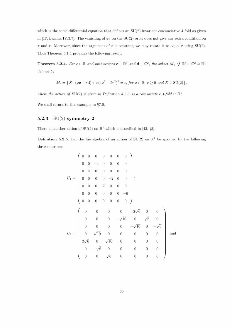
which is the same differential equation that defines an SU(2)-invariant coassociative 4-fold as given
in [17, Lemma IV.3.7]. The vanishing of ϕ0 on the SU(2) orbit does not give any extra condition on
x and r. Moreover, since the argument of z is constant, we may rotate it to equal r using SU(2).
Thus Theorem 5.1.4 provides the following result.
Theorem 5.2.4. For c ∈ R and unit vectors c ∈ R3 and d ∈ C2, the subset Mc of R3 ⊕ C2 ∼= R7
defined by
Mc =X · (xc + rd) : x(4x2 − 5r2)2 = c, for x ∈ R, r ≥ 0 and X ∈ SU(2)
,
where the action of SU(2) is given in Definition 5.2.3, is a coassociative 4-fold in R7.
We shall return to this example in §7.6.
5.2.3 SU(2) symmetry 2
There is another action of SU(2) on R7 which is described in [43, §3].
Definition 5.2.5. Let the Lie algebra of an action of SU(2) on R7 be spanned by the following
three matrices:
U1 =
0 0 0 0 0 0 0
0 0 −4 0 0 0 0
0 4 0 0 0 0 0
0 0 0 0 −2 0 0
0 0 0 2 0 0 0
0 0 0 0 0 0 −6
0 0 0 0 0 6 0
;
U2 =
0 0 0 0 −2√
6 0 0
0 0 0 −√10 0√
6 0
0 0 0 0 −√10 0 −√6
0√
10 0 0 0 0 0
2√
6 0√
10 0 0 0 0
0 −√6 0 0 0 0 0
0 0√
6 0 0 0 0
; and
66
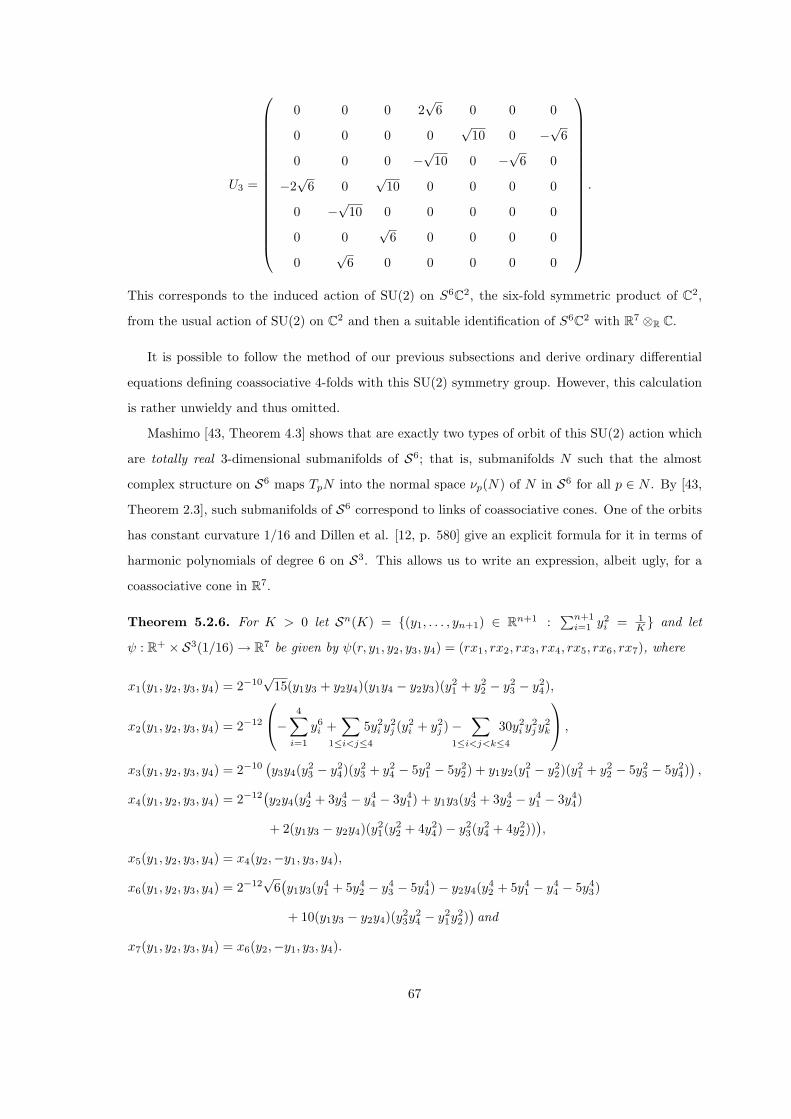
U3 =
0 0 0 2√
6 0 0 0
0 0 0 0√
10 0 −√6
0 0 0 −√10 0 −√6 0
−2√
6 0√
10 0 0 0 0
0 −√10 0 0 0 0 0
0 0√
6 0 0 0 0
0√
6 0 0 0 0 0
.
This corresponds to the induced action of SU(2) on S6C2, the six-fold symmetric product of C2,
from the usual action of SU(2) on C2 and then a suitable identification of S6C2 with R7 ⊗R C.
It is possible to follow the method of our previous subsections and derive ordinary differential
equations defining coassociative 4-folds with this SU(2) symmetry group. However, this calculation
is rather unwieldy and thus omitted.
Mashimo [43, Theorem 4.3] shows that are exactly two types of orbit of this SU(2) action which
are totally real 3-dimensional submanifolds of S6; that is, submanifolds N such that the almost
complex structure on S6 maps TpN into the normal space νp(N) of N in S6 for all p ∈ N . By [43,
Theorem 2.3], such submanifolds of S6 correspond to links of coassociative cones. One of the orbits
has constant curvature 1/16 and Dillen et al. [12, p. 580] give an explicit formula for it in terms of
harmonic polynomials of degree 6 on S3. This allows us to write an expression, albeit ugly, for a
coassociative cone in R7.
Theorem 5.2.6. For K > 0 let Sn(K) = (y1, . . . , yn+1) ∈ Rn+1 :∑n+1
i=1 y2i = 1
K and let
ψ : R+ × S3(1/16) → R7 be given by ψ(r, y1, y2, y3, y4) = (rx1, rx2, rx3, rx4, rx5, rx6, rx7), where
x1(y1, y2, y3, y4) = 2−10√
15(y1y3 + y2y4)(y1y4 − y2y3)(y21 + y2
2 − y23 − y2
4),
x2(y1, y2, y3, y4) = 2−12
−
4∑
i=1
y6i +
∑
1≤i<j≤4
5y2i y2
j (y2i + y2
j )−∑
1≤i<j<k≤4
30y2i y2
j y2k
,
x3(y1, y2, y3, y4) = 2−10(y3y4(y2
3 − y24)(y2
3 + y24 − 5y2
1 − 5y22) + y1y2(y2
1 − y22)(y2
1 + y22 − 5y2
3 − 5y24)
),
x4(y1, y2, y3, y4) = 2−12(y2y4(y4
2 + 3y43 − y4
4 − 3y41) + y1y3(y4
3 + 3y42 − y4
1 − 3y44)
+ 2(y1y3 − y2y4)(y21(y2
2 + 4y24)− y2
3(y24 + 4y2
2))),
x5(y1, y2, y3, y4) = x4(y2,−y1, y3, y4),
x6(y1, y2, y3, y4) = 2−12√
6(y1y3(y4
1 + 5y42 − y4
3 − 5y44)− y2y4(y4
2 + 5y41 − y4
4 − 5y43)
+ 10(y1y3 − y2y4)(y23y2
4 − y21y2
2))and
x7(y1, y2, y3, y4) = x6(y2,−y1, y3, y4).
67

Then M = ψ(R+ × S3(1/16)) is a coassociative cone in R7.
Note that the choice of scaling in Theorem 5.2.6 ensures that ψ(1 × S3(1/16)) ⊆ S6(1).
5.3 Cayley 4-folds with Symmetries
We continue to follow our now familiar construction method, using Lie subgroups of Spin(7) n R8
with a 3-dimensional orbit.
5.3.1 U(1)2-invariant cones
Definition 5.3.1. Let G ⊆ U(1)4 be defined by:
G =(eiα1 , eiα2 , eiα3 , eiα4) : α1, α2, α3, α4 ∈ R satisfying
α1 + α2 + α3 + α4 = 0 and a1α1 + a2α2 + a3α3 + a4α4 = 0
for coprime integers a1, a2, a3, a4 with a1 + a2 + a3 + a4 = 0 and a1 ≤ a2 ≤ a3 ≤ a4. This acts on
C4 ∼= R8 in the obvious way as a U(1)2 subgroup of U(1)4.
We consider G-invariant Cayley cones. Thus define embeddings ψt : R+ ×G → C4 ∼= R8 by:
ψt
(r, (eiα1 , eiα2 , eiα3 , eiα4)
)= (reiα1z1(t), reiα2z2(t), reiα3z3(t), reiα4z4(t)), (5.19)
where z1(t), z2(t), z3(t) and z4(t) are smooth functions of t.
We take our nowhere vanishing 3-vector χ to be:
χ =r
2∂
∂r∧
∑
1≤j<k≤4
(−1)j+k−1(aj − ak) ∂1 ∧ . . . ∧ ∂j−1 ∧ ∂j+1 ∧ . . . ∧ ∂k−1 ∧ ∂k+1 ∧ ∂4, (5.20)
where ∂j = ∂∂αj
. Using the formula (5.19) for ψt we find that
(ψt)∗
(r
∂
∂r
)=
4∑
j=1
(zj
∂
∂zj+ zj
∂
∂zj
)and (ψt)∗(∂j) = izj
∂
∂zj− izj
∂
∂zjfor j = 1, 2, 3, 4.
We may then use these equations to calculate (ψt)∗(χ) from (5.20). Using equation (2.12) for Φ0 we
can calculate the right-hand side of (5.2) and the left-hand side can be written as:
dψt
dt=
4∑
j=1
(dzj
dt
∂
∂zj+
dzj
dt
∂
∂zj
).
Equating both sides of (5.2) and implementing Theorem 5.1.5 gives the following.
68

Theorem 5.3.2. Use the notation of Definition 5.3.1. Let zj : R→ C for j = 1, 2, 3, 4 be differen-
tiable functions satisfying
dz1
dt= a1z2z3z4 +
12
z1
((a4 − a3)|z2|2 + (a2 − a4)|z3|2 + (a3 − a2)|z4|2
), (5.21)
dz2
dt= a2z3z4z1 +
12
z2
((a4 − a1)|z3|2 + (a1 − a3)|z4|2 + (a3 − a4)|z1|2
), (5.22)
dz3
dt= a3z4z1z2 +
12
z3
((a2 − a1)|z4|2 + (a4 − a2)|z1|2 + (a1 − a4)|z2|2
)and (5.23)
dz4
dt= a4z1z2z3 +
12
z4
((a2 − a3)|z1|2 + (a3 − a1)|z2|2 + (a1 − a2)|z3|2
). (5.24)
The subset M of C4 ∼= R8 given by
M =(reiα1z1(t), reiα2z2(t), reiα3z3(t), reiα4z4(t)) : r > 0, (eiα1 , eiα2 , eiα3 , eiα4) ∈ G, t ∈ R
is a Cayley 4-fold in R8. Moreover, |z1|2 + |z2|2 + |z3|2 + |z4|2 is a constant which can be taken to
be 1 and Im(z1z2z3z4) = A for some real constant A.
Proof. Theorem 5.1.5 only gives existence of solutions of t ∈ (−ε, ε) for some ε > 0. However, as in
§4.2.2, we can prove we have solutions that exist for all t ∈ R using the boundedness of the functions
involved. It is clear from (5.21)-(5.24) that |z1|2 + . . . + |z4|2 is a constant and that we can take this
constant to be 1 without loss of generality. Furthermore,
d
dt(z1z2z3z4) = a1|z2z3z4|2 + a2|z3z4z1|2 + a3|z4z1z2|2 + a4|z1z2z3|2,
which is purely real. Therefore Im(z1z2z3z4) = A is constant.
5.3.2 SU(2) symmetry 1
We consider three different natural actions of SU(2) on C4 ∼= R8 in Spin(7). The first is where
SU(2) acts on C4 ∼= C2 ⊕ C2 in the usual manner upon one C2 and trivially upon the other. The
construction using this action gives an affine C2 ⊆ C4 as the Cayley 4-fold. The second is where
SU(2) acts on C4 ∼= C3 ⊕ C as SO(3) on C3 and trivially on C. The construction then produces a
complex surface in C4 as the Cayley 4-fold, which may be written as follows:
(z1, z2, z3, z4) : z2
1 + z22 + z2
3 = A, z4 = B
, where A,B ∈ C are constants.
We therefore turn our attention to the diagonal action of SU(2).
Definition 5.3.3. Let
X =
a b
−b a
∈ SU(2),
69

where a, b ∈ C such that |a|2 + |b|2 = 1. Then X acts on (z1, z2, z3, z4) ∈ C4 ∼= R8 as:
X · (z1, z2, z3, z4) = (az1 + bz2,−bz1 + az2, az3 + bz4,−bz3 + az4).
Define smooth maps ψt : SU(2) → C4 ∼= R8 by:
ψt(X) = X · (z1(t), z2(t), z3(t), z4(t)),
where z1(t), z2(t), z3(t) and z4(t) are smooth functions of t.
Calculation shows that we may take the following three complex matrices as a basis for the Lie
algebra of SU(2) acting in this way:
U1 =
i 0 0 0
0 −i 0 0
0 0 i 0
0 0 0 −i
; U2 =
0 1 0 0
−1 0 0 0
0 0 0 1
0 0 −1 0
; and U3 =
0 i 0 0
i 0 0 0
0 0 0 i
0 0 i 0
.
If we let uj = (ψt)∗(Uj) for j = 1, 2, 3,
u1 = i
(z1
∂
∂z1− z1
∂
∂z1− z2
∂
∂z2+ z2
∂
∂z2+ z3
∂
∂z3− z3
∂
∂z3− z4
∂
∂z4+ z4
∂
∂z4
),
u2 = z2∂
∂z1+ z2
∂
∂z1− z1
∂
∂z2− z1
∂
∂z2+ z4
∂
∂z3+ z4
∂
∂z3− z3
∂
∂z4− z3
∂
∂z4and
u3 = i
(z2
∂
∂z1− z2
∂
∂z1+ z1
∂
∂z2− z1
∂
∂z2+ z4
∂
∂z3− z4
∂
∂z3+ z3
∂
∂z4− z3
∂
∂z4
).
Thus, if we take χ = U1 ∧ U2 ∧ U3, (ψt)∗(χ) = u1 ∧ u2 ∧ u3. Using the equations above for uj and
the formula (2.12) for Φ0, we may calculate the right-hand side of (5.2), which is u1 × u2 × u3 as
defined by (2.14). Moreover,
dψt
dt=
4∑
j=1
dzj
dt
∂
∂zj+
4∑
j=1
dzj
dt
∂
∂zj.
Equating both sides of (5.2) and using Theorem 5.1.5 gives the following result.
Theorem 5.3.4. Let z1(t), z2(t), z3(t), z4(t) be smooth complex-valued functions of t satisfying
dz1
dt= z1
(|z1|2 + |z2|2 + |z3|2 − |z4|2)
+ 2(z1z4 − z2z3 + z2z3)z4, (5.25)
dz2
dt= z2
(|z4|2 + |z1|2 + |z2|2 − |z3|2)− 2(z1z4 − z2z3 − z1z4)z3, (5.26)
dz3
dt= z3
(|z3|2 + |z4|2 + |z1|2 − |z2|2)− 2(z1z4 − z2z3 − z1z4)z2 and (5.27)
dz4
dt= z4
(|z2|2 + |z3|2 + |z4|2 − |z1|2)
+ 2(z1z4 − z2z3 + z2z3)z1 (5.28)
70
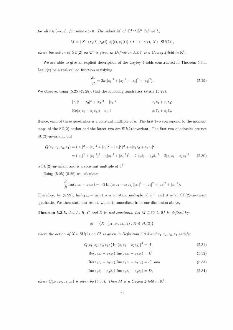
for all t ∈ (−ε, ε), for some ε > 0. The subset M of C4 ∼= R8 defined by
M = X · (z1(t), z2(t), z3(t), z4(t)) : t ∈ (−ε, ε), X ∈ SU(2),
where the action of SU(2) on C4 is given in Definition 5.3.3, is a Cayley 4-fold in R8.
We are able to give an explicit description of the Cayley 4-folds constructed in Theorem 5.3.4.
Let u(t) be a real-valued function satisfying
du
dt= 2u(|z1|2 + |z2|2 + |z3|2 + |z4|2). (5.29)
We observe, using (5.25)-(5.28), that the following quadratics satisfy (5.29):
|z1|2 − |z2|2 + |z3|2 − |z4|2; z1z2 + z3z4;
Re(z1z4 − z2z3); and z1z3 + z2z4.
Hence, each of these quadratics is a constant multiple of u. The first two correspond to the moment
maps of the SU(2) action and the latter two are SU(2)-invariant. The first two quadratics are not
SU(2)-invariant, but
Q(z1, z2, z3, z4) = (|z1|2 − |z2|2 + |z3|2 − |z4|2)2 + 4|z1z2 + z3z4|2
= (|z1|2 + |z2|2)2 + (|z3|2 + |z4|2)2 + 2|z1z3 + z2z4|2 − 2|z1z4 − z2z3|2 (5.30)
is SU(2)-invariant and is a constant multiple of u2.
Using (5.25)-(5.28) we calculate:
d
dtIm(z1z4 − z2z3) = −2 Im(z1z4 − z2z3)(|z1|2 + |z2|2 + |z3|2 + |z4|2).
Therefore, by (5.29), Im(z1z4 − z2z3) is a constant multiple of u−1 and it is an SU(2)-invariant
quadratic. We then state our result, which is immediate from our discussion above.
Theorem 5.3.5. Let A, B, C and D be real constants. Let M ⊆ C4 ∼= R8 be defined by:
M = X · (z1, z2, z3, z4) : X ∈ SU(2),
where the action of X ∈ SU(2) on C4 is given in Definition 5.3.3 and z1, z2, z3, z4 satisfy:
Q(z1, z2, z3, z4)(Im(z1z4 − z2z3)
)2 = A; (5.31)
Re(z1z4 − z2z3) Im(z1z4 − z2z3) = B; (5.32)
Re(z1z3 + z2z4) Im(z1z4 − z2z3) = C; and (5.33)
Im(z1z3 + z2z4) Im(z1z4 − z2z3) = D, (5.34)
where Q(z1, z2, z3, z4) is given by (5.30). Then M is a Cayley 4-fold in R8.
71
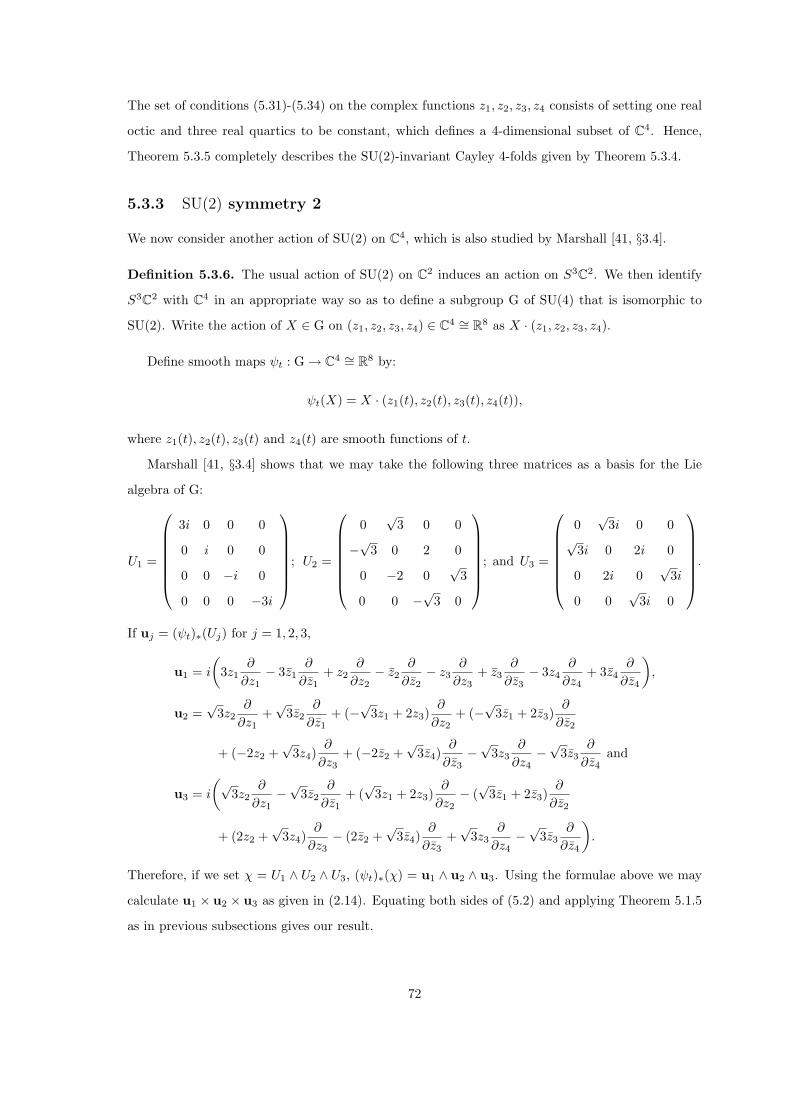
The set of conditions (5.31)-(5.34) on the complex functions z1, z2, z3, z4 consists of setting one real
octic and three real quartics to be constant, which defines a 4-dimensional subset of C4. Hence,
Theorem 5.3.5 completely describes the SU(2)-invariant Cayley 4-folds given by Theorem 5.3.4.
5.3.3 SU(2) symmetry 2
We now consider another action of SU(2) on C4, which is also studied by Marshall [41, §3.4].
Definition 5.3.6. The usual action of SU(2) on C2 induces an action on S3C2. We then identify
S3C2 with C4 in an appropriate way so as to define a subgroup G of SU(4) that is isomorphic to
SU(2). Write the action of X ∈ G on (z1, z2, z3, z4) ∈ C4 ∼= R8 as X · (z1, z2, z3, z4).
Define smooth maps ψt : G → C4 ∼= R8 by:
ψt(X) = X · (z1(t), z2(t), z3(t), z4(t)),
where z1(t), z2(t), z3(t) and z4(t) are smooth functions of t.
Marshall [41, §3.4] shows that we may take the following three matrices as a basis for the Lie
algebra of G:
U1 =
3i 0 0 0
0 i 0 0
0 0 −i 0
0 0 0 −3i
; U2 =
0√
3 0 0
−√3 0 2 0
0 −2 0√
3
0 0 −√3 0
; and U3 =
0√
3i 0 0√
3i 0 2i 0
0 2i 0√
3i
0 0√
3i 0
.
If uj = (ψt)∗(Uj) for j = 1, 2, 3,
u1 = i
(3z1
∂
∂z1− 3z1
∂
∂z1+ z2
∂
∂z2− z2
∂
∂z2− z3
∂
∂z3+ z3
∂
∂z3− 3z4
∂
∂z4+ 3z4
∂
∂z4
),
u2 =√
3z2∂
∂z1+√
3z2∂
∂z1+ (−
√3z1 + 2z3)
∂
∂z2+ (−
√3z1 + 2z3)
∂
∂z2
+ (−2z2 +√
3z4)∂
∂z3+ (−2z2 +
√3z4)
∂
∂z3−√
3z3∂
∂z4−√
3z3∂
∂z4and
u3 = i
(√3z2
∂
∂z1−√
3z2∂
∂z1+ (√
3z1 + 2z3)∂
∂z2− (√
3z1 + 2z3)∂
∂z2
+ (2z2 +√
3z4)∂
∂z3− (2z2 +
√3z4)
∂
∂z3+√
3z3∂
∂z4−√
3z3∂
∂z4
).
Therefore, if we set χ = U1 ∧ U2 ∧ U3, (ψt)∗(χ) = u1 ∧ u2 ∧ u3. Using the formulae above we may
calculate u1 × u2 × u3 as given in (2.14). Equating both sides of (5.2) and applying Theorem 5.1.5
as in previous subsections gives our result.
72
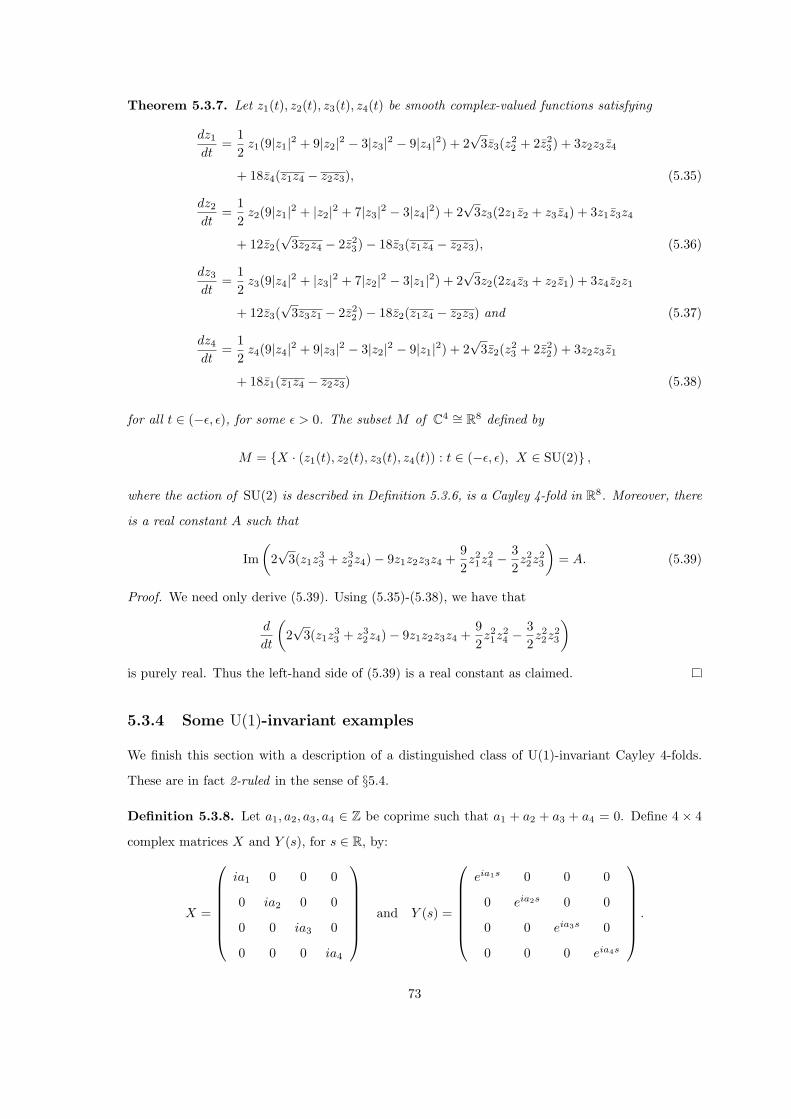
Theorem 5.3.7. Let z1(t), z2(t), z3(t), z4(t) be smooth complex-valued functions satisfying
dz1
dt=
12
z1(9|z1|2 + 9|z2|2 − 3|z3|2 − 9|z4|2) + 2√
3z3(z22 + 2z2
3) + 3z2z3z4
+ 18z4(z1z4 − z2z3), (5.35)
dz2
dt=
12
z2(9|z1|2 + |z2|2 + 7|z3|2 − 3|z4|2) + 2√
3z3(2z1z2 + z3z4) + 3z1z3z4
+ 12z2(√
3z2z4 − 2z23)− 18z3(z1z4 − z2z3), (5.36)
dz3
dt=
12
z3(9|z4|2 + |z3|2 + 7|z2|2 − 3|z1|2) + 2√
3z2(2z4z3 + z2z1) + 3z4z2z1
+ 12z3(√
3z3z1 − 2z22)− 18z2(z1z4 − z2z3) and (5.37)
dz4
dt=
12
z4(9|z4|2 + 9|z3|2 − 3|z2|2 − 9|z1|2) + 2√
3z2(z23 + 2z2
2) + 3z2z3z1
+ 18z1(z1z4 − z2z3) (5.38)
for all t ∈ (−ε, ε), for some ε > 0. The subset M of C4 ∼= R8 defined by
M = X · (z1(t), z2(t), z3(t), z4(t)) : t ∈ (−ε, ε), X ∈ SU(2) ,
where the action of SU(2) is described in Definition 5.3.6, is a Cayley 4-fold in R8. Moreover, there
is a real constant A such that
Im(
2√
3(z1z33 + z3
2z4)− 9z1z2z3z4 +92z21z2
4 −32z22z2
3
)= A. (5.39)
Proof. We need only derive (5.39). Using (5.35)-(5.38), we have that
d
dt
(2√
3(z1z33 + z3
2z4)− 9z1z2z3z4 +92z21z2
4 −32z22z2
3
)
is purely real. Thus the left-hand side of (5.39) is a real constant as claimed.
5.3.4 Some U(1)-invariant examples
We finish this section with a description of a distinguished class of U(1)-invariant Cayley 4-folds.
These are in fact 2-ruled in the sense of §5.4.
Definition 5.3.8. Let a1, a2, a3, a4 ∈ Z be coprime such that a1 + a2 + a3 + a4 = 0. Define 4 × 4
complex matrices X and Y (s), for s ∈ R, by:
X =
ia1 0 0 0
0 ia2 0 0
0 0 ia3 0
0 0 0 ia4
and Y (s) =
eia1s 0 0 0
0 eia2s 0 0
0 0 eia3s 0
0 0 0 eia4s
.
73

Multiplication by Y (s) on C4 corresponds to a U(1) action. Note that Xv is orthogonal to v for
any v ∈ C4.
Define smooth maps ψt : R3 → C4 ∼= R8 by:
ψt(s, λ1, λ2) = Y (s)(λ1v1(t) + λ2v2(t) + w(t)),
where v1,v2,w : R→ C4 are smooth functions.
If we take χ = ∂∂s ∧ ∂
∂λ1∧ ∂
∂λ2, (5.2) becomes:
λ1dv1
dt+ λ2
dv2
dt+
dwdt
= v1 × v2 × (λ1Xv1 + λ2Xv2 + Xw)
for all λ1, λ2 ∈ R, where the triple cross product is defined by (2.14). Applying Theorem 5.1.5 gives
the result below.
Theorem 5.3.9. Use the notation of Definition 5.3.8. Let v1,v2,w : R → C4 be smooth maps,
such that v1(0),v2(0) are orthogonal unit vectors, satisfying
dv1
dt= v1 × v2 ×Xv1,
dv2
dt= v1 × v2 ×Xv2 and
dwdt
= v1 × v2 ×Xw, (5.40)
for t ∈ (−ε, ε), for some ε > 0, where the triple cross product is defined by (2.14). The subset M of
C4 ∼= R8 given by
M = Y (s)(λ1v1(t) + λ2v2(t) + w(t)) : λ1, λ2, s ∈ R, t ∈ (−ε, ε)
is a Cayley 4-fold. Moreover, v1(t) and v2(t) are orthogonal unit vectors for all t ∈ (−ε, ε).
Proof. Theorem 5.1.5 gives existence of the solutions for t ∈ (−ε, ε) for some ε > 0. Recall that the
triple cross product is orthogonal to each of the vectors in the product by Proposition 2.4.2.
Clearly, from (5.40),
g0
(v1,
dv1
dt
)= 0 = g0
(v2,
dv2
dt
).
Thus |v1|2 and |v2|2 are constant and hence equal to 1 since v1(0) and v2(0) are unit vectors.
Furthermore,
d
dtg0(v1,v2) = g0(v1 × v2 ×Xv1,v2) + g0(v1,v1 × v2 ×Xv2) = 0,
which implies that g0(v1,v2) is constant, hence zero by the initial conditions as claimed. This
completes the proof.
74
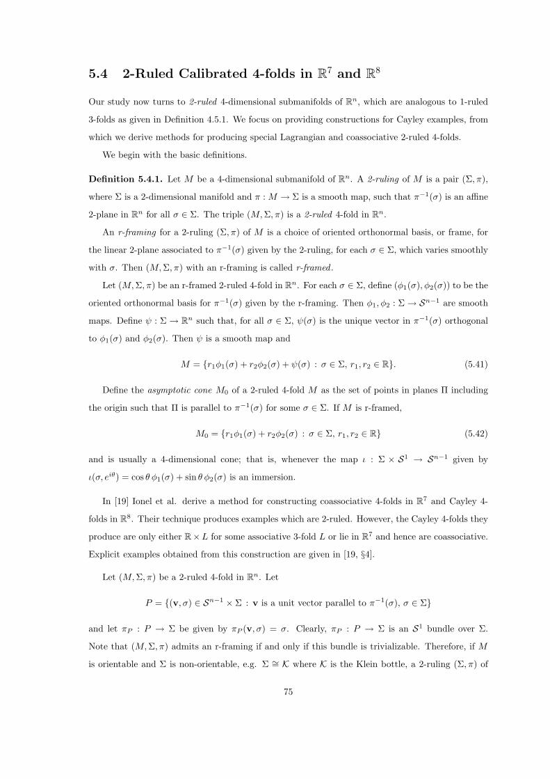
5.4 2-Ruled Calibrated 4-folds in R7 and R8
Our study now turns to 2-ruled 4-dimensional submanifolds of Rn, which are analogous to 1-ruled
3-folds as given in Definition 4.5.1. We focus on providing constructions for Cayley examples, from
which we derive methods for producing special Lagrangian and coassociative 2-ruled 4-folds.
We begin with the basic definitions.
Definition 5.4.1. Let M be a 4-dimensional submanifold of Rn. A 2-ruling of M is a pair (Σ, π),
where Σ is a 2-dimensional manifold and π : M → Σ is a smooth map, such that π−1(σ) is an affine
2-plane in Rn for all σ ∈ Σ. The triple (M, Σ, π) is a 2-ruled 4-fold in Rn.
An r-framing for a 2-ruling (Σ, π) of M is a choice of oriented orthonormal basis, or frame, for
the linear 2-plane associated to π−1(σ) given by the 2-ruling, for each σ ∈ Σ, which varies smoothly
with σ. Then (M, Σ, π) with an r-framing is called r-framed .
Let (M, Σ, π) be an r-framed 2-ruled 4-fold in Rn. For each σ ∈ Σ, define (φ1(σ), φ2(σ)) to be the
oriented orthonormal basis for π−1(σ) given by the r-framing. Then φ1, φ2 : Σ → Sn−1 are smooth
maps. Define ψ : Σ → Rn such that, for all σ ∈ Σ, ψ(σ) is the unique vector in π−1(σ) orthogonal
to φ1(σ) and φ2(σ). Then ψ is a smooth map and
M = r1φ1(σ) + r2φ2(σ) + ψ(σ) : σ ∈ Σ, r1, r2 ∈ R. (5.41)
Define the asymptotic cone M0 of a 2-ruled 4-fold M as the set of points in planes Π including
the origin such that Π is parallel to π−1(σ) for some σ ∈ Σ. If M is r-framed,
M0 = r1φ1(σ) + r2φ2(σ) : σ ∈ Σ, r1, r2 ∈ R (5.42)
and is usually a 4-dimensional cone; that is, whenever the map ι : Σ × S1 → Sn−1 given by
ι(σ, eiθ) = cos θ φ1(σ) + sin θ φ2(σ) is an immersion.
In [19] Ionel et al. derive a method for constructing coassociative 4-folds in R7 and Cayley 4-
folds in R8. Their technique produces examples which are 2-ruled. However, the Cayley 4-folds they
produce are only either R×L for some associative 3-fold L or lie in R7 and hence are coassociative.
Explicit examples obtained from this construction are given in [19, §4].
Let (M, Σ, π) be a 2-ruled 4-fold in Rn. Let
P = (v, σ) ∈ Sn−1 × Σ : v is a unit vector parallel to π−1(σ), σ ∈ Σ
and let πP : P → Σ be given by πP (v, σ) = σ. Clearly, πP : P → Σ is an S1 bundle over Σ.
Note that (M, Σ, π) admits an r-framing if and only if this bundle is trivializable. Therefore, if M
is orientable and Σ is non-orientable, e.g. Σ ∼= K where K is the Klein bottle, a 2-ruling (Σ, π) of
75

M cannot be r-framed. Moreover, if M is r-framed then M0 is not necessarily 4-dimensional. For
example, if we take Σ = R2 and define φ1, φ2 and ψ by φ1(x, y) = (1, 0, 0, 0), φ2(x, y) = (0, 1, 0, 0)
and ψ(x, y) = (0, 0, x, y) for x, y ∈ R, then M , as defined by (5.41), is an r-framed 2-ruled 4-fold
since M = R4, but M0 = R2. We also note that any r-framed 2-ruled 4-fold is defined by three maps
φ1, φ2 and ψ as in (5.41). We may thus construct 2-ruled calibrated 4-folds by formulating partial
differential equations for φ1, φ2 and ψ.
In an analogous manner to the 1-ruled case, one may show that an r-framed 2-ruled 4-fold is
asymptotically conical with rate 0 to its asymptotic cone if Σ is compact.
5.4.1 The partial differential equations
We wish to construct 2-ruled calibrated 4-folds in R7 and R8 by solving partial differential equations
for maps φ1, φ2, ψ. By Propositions 2.4.7 and 3.1.4, it is sufficient to consider the Cayley case.
Let Σ be a 2-dimensional, connected, real analytic manifold, let φ1, φ2 : Σ → S7 be orthogonal
real analytic maps such that ι : Σ × S1 → S7 defined by ι(σ, eiθ) = cos θφ1(σ) + sin θφ2(σ) is an
immersion and let ψ : Σ → R8 be a real analytic map. Clearly, R2 ×Σ is an r-framed 2-ruled 4-fold
with 2-ruling (Σ, π), where π(r1, r2, σ) = σ. Let M be defined by (5.41). Then M is the image of the
map ιM : R2 ×Σ → R8 given by ιM (r1, r2, σ) = r1φ1(σ) + r2φ2(σ) + ψ(σ). Since ι is an immersion,
ιM is an immersion almost everywhere. Thus M is an r-framed 2-ruled 4-fold in R8, possibly with
singularities.
Suppose M is Cayley and p ∈ M . There exist (r1, r2) ∈ R2 and σ ∈ Σ such that p = r1φ1(σ) +
r2φ2(σ) + ψ(σ). Choose oriented coordinates (s, t) near σ in Σ. Then TpM = 〈x,y, z,w〉R, where
x = φ1(σ), y = φ2(σ), z = r1∂φ1
∂s(σ)+r2
∂φ2
∂s(σ)+
∂ψ
∂s(σ) and w = r1
∂φ1
∂t(σ)+r2
∂φ2
∂t(σ)+
∂ψ
∂t(σ).
The tangent space TpM is a Cayley 4-plane. By Proposition 2.4.4 this is true if and only if Im(x×y×z×w) = 0, identifying R8 with O. This implies that a quadratic in r1 and r2 must vanish for all
(r1, r2) ∈ R2, so each coefficient in the quadratic is zero. Therefore, the following set of equations
must hold in Σ:
Im(
φ1 × φ2 × ∂φ1
∂s× ∂φ1
∂t
)= 0; (5.43)
Im(
φ1 × φ2 × ∂φ2
∂s× ∂φ2
∂t
)= 0; (5.44)
Im(
φ1 × φ2 × ∂φ1
∂s× ∂φ2
∂t
)+ Im
(φ1 × φ2 × ∂φ2
∂s× ∂φ1
∂t
)= 0; (5.45)
76

Im(
φ1 × φ2 × ∂ψ
∂s× ∂ψ
∂t
)= 0; (5.46)
Im(
φ1 × φ2 × ∂φ1
∂s× ∂ψ
∂t
)+ Im
(φ1 × φ2 × ∂ψ
∂s× ∂φ1
∂t
)= 0; and (5.47)
Im(
φ1 × φ2 × ∂φ2
∂s× ∂ψ
∂t
)+ Im
(φ1 × φ2 × ∂ψ
∂s× ∂φ2
∂t
)= 0. (5.48)
If we do not suppose M to be Cayley but instead insist that (5.43)-(5.48) hold in Σ then,
following the argument above, each tangent space to M must be Cayley and hence M is a Cayley
4-fold. Noting that (5.43)-(5.45) are precisely the conditions for the asymptotic cone M0 of M to
be Cayley, we deduce the following result.
Proposition 5.4.2. The asymptotic cone of an r-framed 2-ruled Cayley 4-fold in R8 is Cayley
provided it is 4-dimensional.
It is apparent, from consideration of Proposition 2.4.7, that ι(Σ× S1) ⊆ S7 is the link of a Cayley
cone if and only if it is an associative 3-fold in S7.
Clearly, M0 is the image of the map ι0 : R2×Σ → R8 given by ι0(r1, r2, σ) = r1φ1(σ) + r2φ2(σ).
Since we suppose that ι is an immersion, ι0 is an immersion except at (r1, r2) = (0, 0), so M0 is
nonsingular except at 0 and thus is a cone.
Note that Φ0 is a nowhere vanishing 4-form on M0 that defines its orientation, since M0 is Cayley.
Hence, if (s, t) are local coordinates on Σ, we can define them to be oriented by imposing
Φ0
(φ1, φ2, r1
∂φ1
∂s+ r2
∂φ2
∂s, r1
∂φ1
∂t+ r2
∂φ2
∂t
)> 0 (5.49)
for all (r1, r2) ∈ R2 \ (0, 0). It follows that
Φ0
(φ1, φ2,
∂φ1
∂s,∂φ1
∂t
)> 0 and Φ0
(φ1, φ2,
∂φ2
∂s,∂φ2
∂t
)> 0. (5.50)
Consequently, φ1, φ2,∂φj
∂s ,∂φj
∂t is a linearly independent set for j = 1, 2. Moreover, (5.49) is
equivalent to the condition that ι is an immersion.
We now construct a metric on Σ, under suitable conditions, using φ1, φ2 and the metric on R8.
For a function f : Σ → R8, we define f⊥ : Σ → R8 by choosing f⊥(σ) to be the component of
f(σ) that lies in the orthogonal complement of 〈φ1(σ), φ2(σ)〉R. Since the fourfold cross product is
alternating, (5.43)-(5.45) hold if and only if
Im
(φ1 × φ2 ×
(cos θ
∂φ1
∂s
⊥+ sin θ
∂φ2
∂s
⊥)×
(cos θ
∂φ1
∂t
⊥+ sin θ
∂φ2
∂t
⊥))= 0 (5.51)
for all θ ∈ R. Let σ ∈ Σ. From Proposition 2.4.4 and (5.49) we see that, for each θ ∈ R, the four
terms in (5.51), evaluated at σ, form a basis for a Cayley 4-plane Πθ. By Corollary 2.4.5, we may
77

also take(
φ1(σ), φ2(σ), cos θ∂φ1
∂s
⊥(σ) + sin θ
∂φ2
∂s
⊥(σ), cos θφ1 × φ2 × ∂φ1
∂s
⊥(σ) + sin θφ1 × φ2 × ∂φ2
∂s
⊥(σ)
)
as a basis for Πθ. Therefore,
cos θ∂φ1
∂t
⊥(σ) + sin θ
∂φ2
∂t
⊥(σ) = Aθ
(cos θ
∂φ1
∂s
⊥(σ) + sin θ
∂φ2
∂s
⊥(σ)
)
+ Bθ
(cos θφ1 × φ2 × ∂φ1
∂s
⊥(σ) + sin θφ1 × φ2 × ∂φ2
∂s
⊥(σ)
)(5.52)
for constants Aθ, Bθ depending on θ. We set θ = 0, π2 in (5.52) and substitute back in the expressions
found for the t derivatives to obtain:
cos θ
((A0 −Aθ)
∂φ1
∂s
⊥(σ) + (B0 −Bθ)φ1 × φ2 × ∂φ1
∂s
⊥(σ)
)=
sin θ
((Aθ −Aπ
2)∂φ2
∂s
⊥(σ) + (Bθ −Bπ
2)φ1 × φ2 × ∂φ2
∂s
⊥(σ)
). (5.53)
To proceed in defining a metric on Σ we impose a condition on the dimension of
Vσ =
⟨∂φ1
∂s
⊥(σ),
∂φ2
∂s
⊥(σ), φ1 × φ2 × ∂φ1
∂s
⊥(σ), φ1 × φ2 × ∂φ2
∂s
⊥(σ)
⟩
R.
Let Wσ = 〈φ1(σ), φ2(σ)〉⊥R ⊆ R8 and define Jσ : Wσ → Wσ by Jσ(v) = φ1(σ) × φ2(σ) × v. It is
clear, through calculation in coordinates, that J2σ = −1 on Wσ. Note that Vσ ⊆ Wσ is closed under
the action of Jσ, which can thus be considered as a form of complex structure on Vσ. Hence, Vσ is
even-dimensional. Since the case dim Vσ = 0 is excluded by (5.50), dimVσ = 2 or 4. Recall that Σ
is real analytic and connected. Therefore σ ∈ Σ : dim Vσ = 2 is a closed real analytic subset of Σ
and consequently either coincides with Σ or is of zero measure in Σ.
Suppose that dim Vσ = 4. The four vectors in (5.53) are then linearly independent and hence
(A0 −Aθ) cos θ = (B0 −Bθ) cos θ = (Aπ2−Aθ) sin θ = (Bπ
2−Bθ) sin θ = 0
for all θ. This clearly forces Aθ and Bθ to be constant and equal to A and B, say, respectively.
Define a metric gΣ pointwise on Σ, up to scale, by the following equations:
gΣ
(∂
∂s,
∂
∂t
)= AgΣ
(∂
∂s,
∂
∂s
)and gΣ
(∂
∂t,
∂
∂t
)= (A2 + B2)gΣ
(∂
∂s,
∂
∂s
). (5.54)
Using (5.52) and the fact that J2σ = −1 on Vσ,
φ1 × φ2 × ∂φj
∂s
⊥(σ)
φ1 × φ2 × ∂φj
∂t
⊥(σ)
= K
∂φj
∂s
⊥(σ)
∂φj
∂t
⊥(σ)
78

for j = 1, 2, where K is the 2× 2 matrix given by:
K =1B
−A 1
−(A2 + B2) A
.
If we change coordinates (s, t) to (s, t) with Jacobian matrix L, K transforms to K = LKL−1.
Calculation shows that the corresponding A and B defining K satisfy (5.54) for the coordinates
(s, t). Thus, gΣ is a well-defined metric, up to scale, covariant under transformation of coordinates.
Having defined the metric gΣ we can consider Σ as a Riemannian 2-fold, which has a natural
orientation derived from the orientation on M and on the 2-planes 〈φ1(σ), φ2(σ)〉R. Therefore it
has a natural complex structure which we denote as J . If we choose a local holomorphic coordinate
u = s + it on Σ, the corresponding real coordinates must satisfy ∂∂t = J ∂
∂s . We say that local real
coordinates (s, t) on Σ satisfying this condition are oriented conformal coordinates as in §4.5.1. This
forces A = 0 and B = 1 in the notation of (5.54), since B > 0 by (5.50).
We now state and prove a theorem in this case.
Theorem 5.4.3. Let Σ be a connected real analytic 2-fold, let φ1, φ2 : Σ → S7 be orthogonal real
analytic maps such that ι : Σ×S1 → S7 defined by ι(σ, eiθ) = cos θφ1(σ)+sin θφ2(σ) is an immersion,
and let ψ : Σ → R8 be a real analytic map. Define M by (5.41) and suppose that dim Vσ = 4 almost
everywhere in Σ. Then M is Cayley if and only if
∂φ1
∂t= φ1 × φ2 × ∂φ1
∂s+ fφ2, (5.55)
∂φ2
∂t= φ1 × φ2 × ∂φ2
∂s− fφ1, (5.56)
for some function f : Σ → R, and ψ satisfies
∂ψ
∂t= φ1 × φ2 × ∂ψ
∂s+ g1φ1 + g2φ2 (5.57)
for some functions g1, g2 : Σ → R, where the triple cross product is defined in (2.14) and (s, t) are
oriented conformal coordinates on Σ. Moreover, sufficiency holds irrespective of dim Vσ.
Proof. Recalling that (5.43)-(5.48) correspond to the condition that M is Cayley, we show that
(5.43)-(5.45) are equivalent to (5.55)-(5.56), and that (5.46)-(5.48) are equivalent to (5.57).
Let σ ∈ Σ. Since φ1 maps to S7 it is clear that φ1(σ) is orthogonal to ∂φ1∂s (σ) and ∂φ1
∂t (σ). By
(5.52) and the work above, there exist a1, a2, a3 ∈ R such that
∂φ1
∂t(σ) = a1φ1 × φ2 × ∂φ1
∂s(σ) + a2φ2(σ) + a3
∂φ1
∂s(σ). (5.58)
We then calculate:
g0
(∂φ1
∂t
⊥(σ),
∂φ1
∂s
⊥(σ)
)= a3
∣∣∣∣∣∂φ1
∂s
⊥(σ)
∣∣∣∣∣
2
.
79

The left-hand side is zero by (5.54) since (s, t) are oriented conformal coordinates, and hence a3 = 0.
Moreover, following a straightforward calculation,∣∣∣∣∣∂φ1
∂t
⊥(σ)
∣∣∣∣∣
2
= a21
∣∣∣∣ φ1 × φ2 × ∂φ1
∂s(σ)
∣∣∣∣2
= a21
∣∣∣∣∣∂φ1
∂s
⊥(σ)
∣∣∣∣∣
2
and thus a21 = 1 by (5.54). Taking the inner product of (5.58) with the triple cross product gives:
∣∣∣∣ φ1 × φ2 × ∂φ1
∂s(σ)
∣∣∣∣2
a1 = g0
(∂φ1
∂t(σ), φ1 × φ2 × ∂φ1
∂s(σ)
)= Φ0
(φ1(σ), φ2(σ),
∂φ1
∂s(σ),
∂φ1
∂t(σ)
),
using equation (2.13). Therefore a1 > 0 by equation (5.50). Hence a1 = 1 and (5.55) holds
at σ with f(σ) = a2. If (5.55) holds at σ then, by Corollary 2.4.5, the 4-plane spanned by
φ1(σ), φ2(σ), ∂φ1∂s (σ), ∂φ1
∂t (σ) is Cayley.
Similarly, we deduce that (5.44) holding at σ is equivalent to
∂φ2
∂t= φ1 × φ2 × ∂φ2
∂s+ f ′φ1
at σ, for some function f ′ : Σ → R. However,
∂
∂tg0(φ1, φ2) = g0
(∂φ1
∂t, φ2
)+ g0
(φ1,
∂φ2
∂t
)= 0
and so f ′ = −f .
Let (e1, . . . , e8) be the standard orthonormal basis of R8, identified with O such that e1 corre-
sponds to 1 and (e2, . . . , e8) corresponds to the basis of ImO described in §2.1.1. It follows from
[17, Theorem IV.1.38] that Spin(7) acts transitively upon oriented orthonormal bases of Cayley 4-
planes. Hence, we can transform coordinates on R8 using Spin(7) such that a Cayley 4-plane has
basis (e1, e2, e3, e4). Moreover, any orthonormal pair can be mapped to (e1, e2).
By the remarks above, transform coordinates on R8 using Spin(7) such that
φ1(σ) = e1, φ2(σ) = e2,∂φ1
∂s(σ) = b1e1 + . . . + b8e8 and
∂φ2
∂s(σ) = b′1e1 + . . . + b′8e8
for some real constants bj and b′j . If (5.55) and (5.56) hold, we may calculate ∂φ1∂t (σ) and ∂φ2
∂t (σ). A
straightforward calculation in coordinates then shows that (5.43)-(5.45) hold at σ. Since the triple
cross product is invariant under Spin(7) by Definition 2.1.10, we conclude that (5.43)-(5.45) are
equivalent to (5.55) and (5.56).
Suppose now that (5.46)-(5.48) hold at σ ∈ Σ. Using Spin(7), transform coordinates such that
φ1(σ) = e1, φ2(σ) = e2 and∂φ1
∂s(σ) = b1e1 + . . . + b4e4,
where b1, . . . , b4 are real constants, which we are free to do by (5.43). In these coordinates write
∂ψ
∂s(σ) = c1e1 + . . . + c8e8 and
∂ψ
∂t(σ) = d1e1 + . . . + d8e8.
80
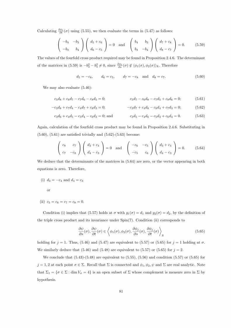
Calculating ∂φ1∂t (σ) using (5.55), we then evaluate the terms in (5.47) as follows:
−b4 −b3
−b3 b4
d5 + c6
d6 − c5
= 0 and
b4 b3
b3 −b4
d7 + c8
d8 − c7
= 0. (5.59)
The values of the fourfold cross product required may be found in Proposition 2.4.6. The determinant
of the matrices in (5.59) is −b23 − b2
4 6= 0, since ∂φ1∂s (σ) /∈ 〈φ1(σ), φ2(σ)〉R. Therefore
d5 = −c6, d6 = c5, d7 = −c8 and d8 = c7. (5.60)
We may also evaluate (5.46):
c5d8 + c6d7 − c7d6 − c8d5 = 0; c5d7 − c6d8 − c7d5 + c8d6 = 0; (5.61)
−c3d8 + c7d4 − c4d7 + c8d3 = 0; −c3d7 + c4d8 − c8d4 + c7d3 = 0; (5.62)
c3d6 + c4d5 − c5d4 − c6d3 = 0; and c3d5 − c4d6 − c5d3 + c6d4 = 0. (5.63)
Again, calculation of the fourfold cross product may be found in Proposition 2.4.6. Substituting in
(5.60), (5.61) are satisfied trivially and (5.62)-(5.63) become: c8 c7
c7 −c8
d3 + c4
d4 − c3
= 0 and
−c6 −c5
−c5 c6
d3 + c4
d4 − c3
= 0. (5.64)
We deduce that the determinants of the matrices in (5.64) are zero, or the vector appearing in both
equations is zero. Therefore,
(i) d3 = −c4 and d4 = c3
or
(ii) c5 = c6 = c7 = c8 = 0.
Condition (i) implies that (5.57) holds at σ with g1(σ) = d1 and g2(σ) = d2, by the definition of
the triple cross product and its invariance under Spin(7). Condition (ii) corresponds to
∂ψ
∂s(σ),
∂ψ
∂t(σ) ∈
⟨φ1(σ), φ2(σ),
∂φj
∂s(σ),
∂φj
∂t(σ)
⟩
R(5.65)
holding for j = 1. Thus, (5.46) and (5.47) are equivalent to (5.57) or (5.65) for j = 1 holding at σ.
We similarly deduce that (5.46) and (5.48) are equivalent to (5.57) or (5.65) for j = 2.
We conclude that (5.43)-(5.48) are equivalent to (5.55), (5.56) and condition (5.57) or (5.65) for
j = 1, 2 at each point σ ∈ Σ. Recall that Σ is connected and φ1, φ2, ψ and Σ are real analytic. Note
that Σ1 = σ ∈ Σ : dim Vσ = 4 is an open subset of Σ whose complement is measure zero in Σ by
hypothesis.
81

Let σ ∈ Σ1 and suppose that (5.65) holds for j = 1, 2 at σ. Then there exist real constants Cjk,
for j = 1, 2 and 1 ≤ k ≤ 4, such that
∂ψ
∂s(σ) = Cj1φ1(σ) + Cj2φ2(σ) + Cj3
∂φj
∂s
⊥(σ) + Cj4
∂φj
∂t
⊥(σ).
Clearly, C1k = C2k for k = 1, 2 by the definition of g⊥ for a function g. Since dim Vσ = 4 ensures the
linear independence of the partial derivatives of φ1 and φ2, Cjk = 0 for j = 1, 2 and k = 3, 4. Hence,∂ψ∂s (σ) and, similarly, ∂ψ
∂t (σ) lie in 〈φ1(σ), φ2(σ)〉R for almost all σ ∈ Σ. Thus ψ satisfies (5.57).
Consequently, (5.57) holds in Σ1. Moreover, Σ2 = σ ∈ Σ : (5.57) holds at σ is a closed real
analytic subset of Σ and so must either coincide with Σ or be of zero measure in Σ. Since Σ1 ⊆ Σ2,
Σ2 cannot be measure zero and so must equal Σ. This completes the proof.
Note that (5.57) is a linear condition on ψ given φ1 and φ2, and that (5.55) and (5.56) are
equivalent to the fact that the asymptotic cone M0 of M is Cayley. Therefore, if we are given an
r-framed 2-ruled Cayley cone M0 defined by φ1 and φ2, any solution ψ of (5.57), together with φ1
and φ2, defines an r-framed 2-ruled Cayley 4-fold with asymptotic cone M0. Moreover, (5.57) is
unchanged if φ1 and φ2 are fixed and satisfy (5.55) and (5.56), but ψ is replaced by ψ + g1φ1 + g2φ2
for real analytic maps g1 and g2. We can thus locally transform ψ, if we relax the condition that ψ
is orthogonal to φ1 and φ2, such that g1 and g2 are zero.
If we suppose instead that dim Vσ = 2 for all σ ∈ Σ then we are unable, in general, to define
a suitable metric and hence oriented conformal coordinates on Σ. However, we shall show that if
we exclude planar r-framed 2-ruled 4-folds, (5.55)-(5.57) of Theorem 5.4.3 characterize the Cayley
condition on φ1, φ2 and ψ and there is a natural conformal structure on Σ.
5.4.2 Gauge transformations
Let φ1 and φ2 satisfy (5.55) and (5.56) in Theorem 5.4.3 for some map f . Taking the triple cross
product of (5.55) and (5.56) with φ1 and φ2 gives:
∂φ1
∂s= −φ1 × φ2 × ∂φ1
∂t+ f
′φ2 and
∂φ2
∂s= −φ1 × φ2 × ∂φ2
∂t− f
′φ1, (5.66)
for some function f′: Σ → R since φ1× φ2× (φ1× φ2× v) = −v for any v orthogonal to φ1 and φ2.
We are allowed to perform a rotation Θ(σ) to the (φ1(σ), φ2(σ))-plane at each point σ ∈ Σ as long
as the function Θ is smooth. The choice of Θ will then alter f and f′. We call such a transformation
a gauge transformation.
We now show that under certain conditions there exists a gauge transformation such that f =
82
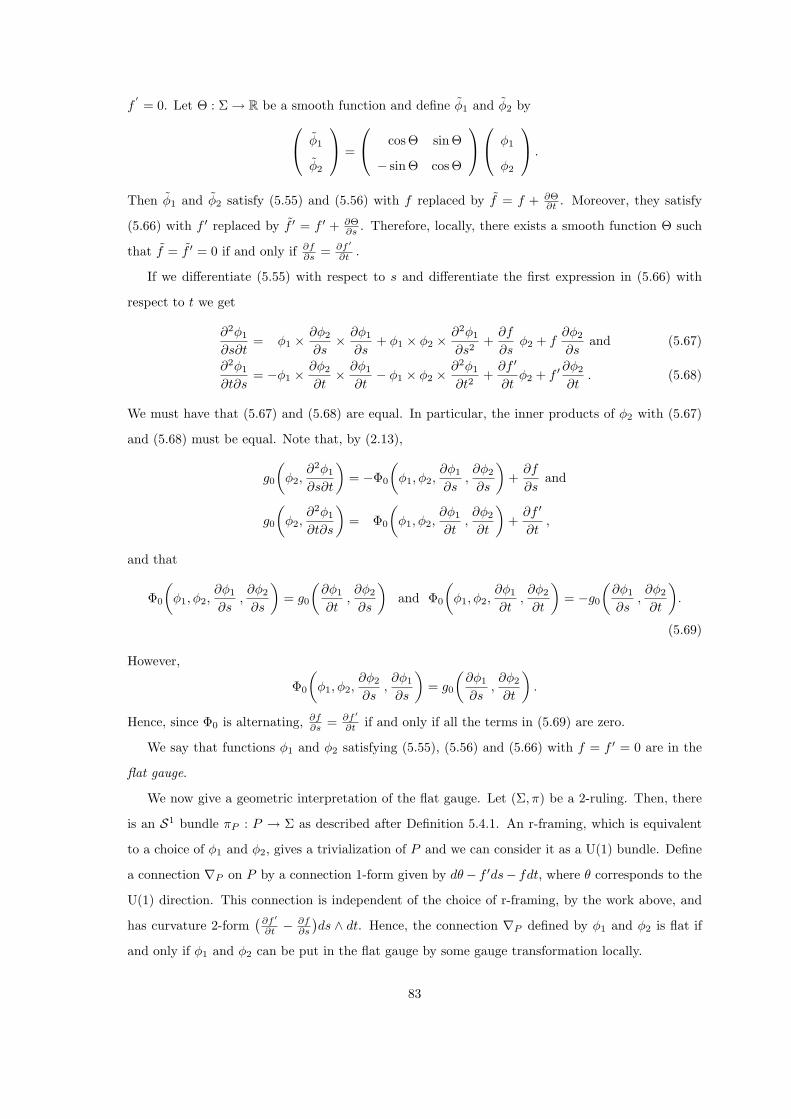
f′= 0. Let Θ : Σ → R be a smooth function and define φ1 and φ2 by
φ1
φ2
=
cosΘ sin Θ
− sinΘ cosΘ
φ1
φ2
.
Then φ1 and φ2 satisfy (5.55) and (5.56) with f replaced by f = f + ∂Θ∂t . Moreover, they satisfy
(5.66) with f ′ replaced by f ′ = f ′ + ∂Θ∂s . Therefore, locally, there exists a smooth function Θ such
that f = f ′ = 0 if and only if ∂f∂s = ∂f ′
∂t .
If we differentiate (5.55) with respect to s and differentiate the first expression in (5.66) with
respect to t we get
∂2φ1
∂s∂t= φ1 × ∂φ2
∂s× ∂φ1
∂s+ φ1 × φ2 × ∂2φ1
∂s2+
∂f
∂sφ2 + f
∂φ2
∂sand (5.67)
∂2φ1
∂t∂s= −φ1 × ∂φ2
∂t× ∂φ1
∂t− φ1 × φ2 × ∂2φ1
∂t2+
∂f ′
∂tφ2 + f ′
∂φ2
∂t. (5.68)
We must have that (5.67) and (5.68) are equal. In particular, the inner products of φ2 with (5.67)
and (5.68) must be equal. Note that, by (2.13),
g0
(φ2,
∂2φ1
∂s∂t
)= −Φ0
(φ1, φ2,
∂φ1
∂s,∂φ2
∂s
)+
∂f
∂sand
g0
(φ2,
∂2φ1
∂t∂s
)= Φ0
(φ1, φ2,
∂φ1
∂t,∂φ2
∂t
)+
∂f ′
∂t,
and that
Φ0
(φ1, φ2,
∂φ1
∂s,∂φ2
∂s
)= g0
(∂φ1
∂t,∂φ2
∂s
)and Φ0
(φ1, φ2,
∂φ1
∂t,∂φ2
∂t
)= −g0
(∂φ1
∂s,∂φ2
∂t
).
(5.69)
However,
Φ0
(φ1, φ2,
∂φ2
∂s,∂φ1
∂s
)= g0
(∂φ1
∂s,∂φ2
∂t
).
Hence, since Φ0 is alternating, ∂f∂s = ∂f ′
∂t if and only if all the terms in (5.69) are zero.
We say that functions φ1 and φ2 satisfying (5.55), (5.56) and (5.66) with f = f ′ = 0 are in the
flat gauge.
We now give a geometric interpretation of the flat gauge. Let (Σ, π) be a 2-ruling. Then, there
is an S1 bundle πP : P → Σ as described after Definition 5.4.1. An r-framing, which is equivalent
to a choice of φ1 and φ2, gives a trivialization of P and we can consider it as a U(1) bundle. Define
a connection ∇P on P by a connection 1-form given by dθ− f ′ds− fdt, where θ corresponds to the
U(1) direction. This connection is independent of the choice of r-framing, by the work above, and
has curvature 2-form(
∂f ′
∂t − ∂f∂s
)ds ∧ dt. Hence, the connection ∇P defined by φ1 and φ2 is flat if
and only if φ1 and φ2 can be put in the flat gauge by some gauge transformation locally.
83
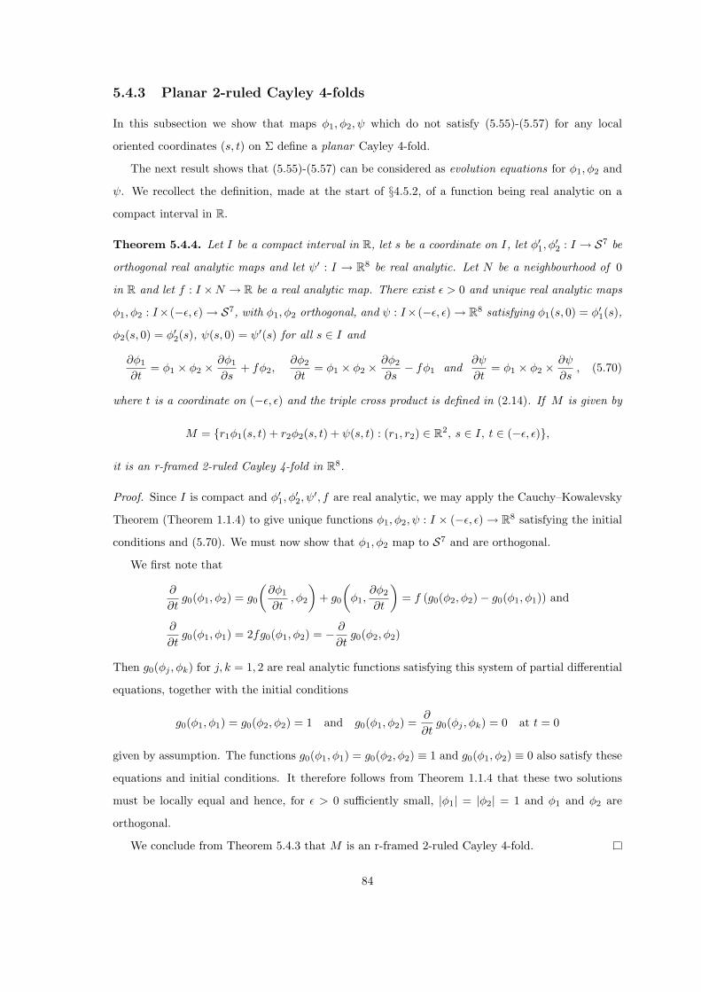
5.4.3 Planar 2-ruled Cayley 4-folds
In this subsection we show that maps φ1, φ2, ψ which do not satisfy (5.55)-(5.57) for any local
oriented coordinates (s, t) on Σ define a planar Cayley 4-fold.
The next result shows that (5.55)-(5.57) can be considered as evolution equations for φ1, φ2 and
ψ. We recollect the definition, made at the start of §4.5.2, of a function being real analytic on a
compact interval in R.
Theorem 5.4.4. Let I be a compact interval in R, let s be a coordinate on I, let φ′1, φ′2 : I → S7 be
orthogonal real analytic maps and let ψ′ : I → R8 be real analytic. Let N be a neighbourhood of 0
in R and let f : I ×N → R be a real analytic map. There exist ε > 0 and unique real analytic maps
φ1, φ2 : I×(−ε, ε) → S7, with φ1, φ2 orthogonal, and ψ : I×(−ε, ε) → R8 satisfying φ1(s, 0) = φ′1(s),
φ2(s, 0) = φ′2(s), ψ(s, 0) = ψ′(s) for all s ∈ I and
∂φ1
∂t= φ1 × φ2 × ∂φ1
∂s+ fφ2,
∂φ2
∂t= φ1 × φ2 × ∂φ2
∂s− fφ1 and
∂ψ
∂t= φ1 × φ2 × ∂ψ
∂s, (5.70)
where t is a coordinate on (−ε, ε) and the triple cross product is defined in (2.14). If M is given by
M = r1φ1(s, t) + r2φ2(s, t) + ψ(s, t) : (r1, r2) ∈ R2, s ∈ I, t ∈ (−ε, ε),
it is an r-framed 2-ruled Cayley 4-fold in R8.
Proof. Since I is compact and φ′1, φ′2, ψ
′, f are real analytic, we may apply the Cauchy–Kowalevsky
Theorem (Theorem 1.1.4) to give unique functions φ1, φ2, ψ : I × (−ε, ε) → R8 satisfying the initial
conditions and (5.70). We must now show that φ1, φ2 map to S7 and are orthogonal.
We first note that
∂
∂tg0(φ1, φ2) = g0
(∂φ1
∂t, φ2
)+ g0
(φ1,
∂φ2
∂t
)= f (g0(φ2, φ2)− g0(φ1, φ1)) and
∂
∂tg0(φ1, φ1) = 2fg0(φ1, φ2) = − ∂
∂tg0(φ2, φ2)
Then g0(φj , φk) for j, k = 1, 2 are real analytic functions satisfying this system of partial differential
equations, together with the initial conditions
g0(φ1, φ1) = g0(φ2, φ2) = 1 and g0(φ1, φ2) =∂
∂tg0(φj , φk) = 0 at t = 0
given by assumption. The functions g0(φ1, φ1) = g0(φ2, φ2) ≡ 1 and g0(φ1, φ2) ≡ 0 also satisfy these
equations and initial conditions. It therefore follows from Theorem 1.1.4 that these two solutions
must be locally equal and hence, for ε > 0 sufficiently small, |φ1| = |φ2| = 1 and φ1 and φ2 are
orthogonal.
We conclude from Theorem 5.4.3 that M is an r-framed 2-ruled Cayley 4-fold.
84
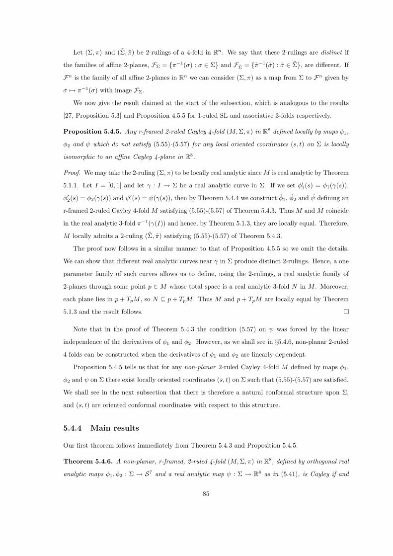
Let (Σ, π) and (Σ, π) be 2-rulings of a 4-fold in Rn. We say that these 2-rulings are distinct if
the families of affine 2-planes, FΣ = π−1(σ) : σ ∈ Σ and FΣ = π−1(σ) : σ ∈ Σ, are different. If
Fn is the family of all affine 2-planes in Rn we can consider (Σ, π) as a map from Σ to Fn given by
σ 7→ π−1(σ) with image FΣ.
We now give the result claimed at the start of the subsection, which is analogous to the results
[27, Proposition 5.3] and Proposition 4.5.5 for 1-ruled SL and associative 3-folds respectively.
Proposition 5.4.5. Any r-framed 2-ruled Cayley 4-fold (M, Σ, π) in R8 defined locally by maps φ1,
φ2 and ψ which do not satisfy (5.55)-(5.57) for any local oriented coordinates (s, t) on Σ is locally
isomorphic to an affine Cayley 4-plane in R8.
Proof. We may take the 2-ruling (Σ, π) to be locally real analytic since M is real analytic by Theorem
5.1.1. Let I = [0, 1] and let γ : I → Σ be a real analytic curve in Σ. If we set φ′1(s) = φ1(γ(s)),
φ′2(s) = φ2(γ(s)) and ψ′(s) = ψ(γ(s)), then by Theorem 5.4.4 we construct φ1, φ2 and ψ defining an
r-framed 2-ruled Cayley 4-fold M satisfying (5.55)-(5.57) of Theorem 5.4.3. Thus M and M coincide
in the real analytic 3-fold π−1(γ(I)) and hence, by Theorem 5.1.3, they are locally equal. Therefore,
M locally admits a 2-ruling (Σ, π) satisfying (5.55)-(5.57) of Theorem 5.4.3.
The proof now follows in a similar manner to that of Proposition 4.5.5 so we omit the details.
We can show that different real analytic curves near γ in Σ produce distinct 2-rulings. Hence, a one
parameter family of such curves allows us to define, using the 2-rulings, a real analytic family of
2-planes through some point p ∈ M whose total space is a real analytic 3-fold N in M . Moreover,
each plane lies in p + TpM , so N ⊆ p + TpM . Thus M and p + TpM are locally equal by Theorem
5.1.3 and the result follows.
Note that in the proof of Theorem 5.4.3 the condition (5.57) on ψ was forced by the linear
independence of the derivatives of φ1 and φ2. However, as we shall see in §5.4.6, non-planar 2-ruled
4-folds can be constructed when the derivatives of φ1 and φ2 are linearly dependent.
Proposition 5.4.5 tells us that for any non-planar 2-ruled Cayley 4-fold M defined by maps φ1,
φ2 and ψ on Σ there exist locally oriented coordinates (s, t) on Σ such that (5.55)-(5.57) are satisfied.
We shall see in the next subsection that there is therefore a natural conformal structure upon Σ,
and (s, t) are oriented conformal coordinates with respect to this structure.
5.4.4 Main results
Our first theorem follows immediately from Theorem 5.4.3 and Proposition 5.4.5.
Theorem 5.4.6. A non-planar, r-framed, 2-ruled 4-fold (M, Σ, π) in R8, defined by orthogonal real
analytic maps φ1, φ2 : Σ → S7 and a real analytic map ψ : Σ → R8 as in (5.41), is Cayley if and
85

only if there exist locally oriented coordinates (s, t) on Σ such that φ1, φ2 and ψ satisfy (5.55)-(5.57)
for some real analytic functions f, g1, g2 : Σ → R.
We now prove the result claimed at the end of the last subsection.
Proposition 5.4.7. Let (M, Σ, π) be a non-planar, r-framed, 2-ruled Cayley 4-fold in R8. There
exists a unique conformal structure on Σ with respect to which (s, t) as given in Theorem 5.4.6 are
oriented conformal coordinates.
Proof. Let (s, t) be local oriented coordinates as given by Theorem 5.4.6. Define a complex structure
J on Σ by requiring that u = s + it is a holomorphic coordinate on Σ, i.e. that ∂∂t = J ∂
∂s . Note
that, by (5.55)-(5.56) and (5.66), φ1 and φ2 as given in Theorem 5.4.6 satisfy
∂φj
∂t
⊥= φ1 × φ2 × ∂φj
∂s
⊥and
∂φj
∂s
⊥= −φ1 × φ2 × ∂φj
∂t
⊥for j = 1, 2. (5.71)
Suppose that (s, t) are local oriented coordinates on Σ such that φ1 and φ2 also satisfy (5.55)-(5.56)
in these coordinates. Hence, φ1 and φ2 satisfy (5.71) for the coordinates (s, t).
We calculate:
∂φj
∂t
⊥=
∂s
∂t
∂φj
∂s
⊥+
∂t
∂t
∂φj
∂t
⊥= φ1 × φ2 ×
(∂t
∂t
∂φj
∂s
⊥− ∂s
∂t
∂φj
∂t
⊥)
and
∂φj
∂s
⊥=
∂s
∂s
∂φj
∂s
⊥+
∂t
∂s
∂φj
∂t
⊥.
Note that, from (5.71), ∂φj
∂t
⊥is orthogonal to ∂φj
∂s
⊥and, moreover, that ∂φj
∂t
⊥ 6= 0 if and only if∂φj
∂s
⊥ 6= 0 by the definition of f⊥ for a function f : Σ → R and the properties of the triple cross
product. Using (5.71) for (s, t) we deduce that
∂s
∂s=
∂t
∂tand
∂s
∂t= − ∂t
∂s, (5.72)
since not both ∂φ1∂s
⊥and ∂φ2
∂s
⊥are zero.
Therefore, using (5.72),
∂
∂t=
∂s
∂t
∂
∂s+
∂t
∂t
∂
∂t= − ∂t
∂s
∂
∂s+
∂s
∂s
∂
∂t= J
(∂t
∂s
∂
∂t+
∂s
∂s
∂
∂s
)= J
∂
∂s.
Hence we have the result.
It is clear that the conformal structure given by Proposition 5.4.7 coincides with the one given by
the metric as described in the preamble to Theorem 5.4.3.
We now use Propositions 2.4.7 and 3.1.4 to prove analogous results for coassociative 4-folds in
R7 and SL 4-folds in C4. We begin with the SL case, for which we recall the triple cross product on
C4 described in Definition 3.1.8.
86
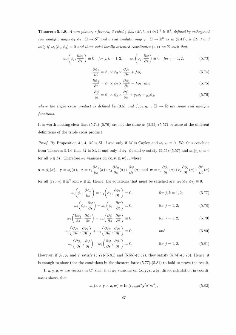
Theorem 5.4.8. A non-planar, r-framed, 2-ruled 4-fold (M, Σ, π) in C4 ∼= R8, defined by orthogonal
real analytic maps φ1, φ2 : Σ → S7 and a real analytic map ψ : Σ → R8 as in (5.41), is SL if and
only if ω4(φ1, φ2) ≡ 0 and there exist locally oriented coordinates (s, t) on Σ such that:
ω4
(φj ,
∂φk
∂s
)≡ 0 for j, k = 1, 2; ω4
(φj ,
∂ψ
∂s
)≡ 0 for j = 1, 2; (5.73)
∂φ1
∂t= φ1 × φ2 × ∂φ1
∂s+ fφ2; (5.74)
∂φ2
∂t= φ1 × φ2 × ∂φ2
∂s− fφ1; and (5.75)
∂ψ
∂t= φ1 × φ2 × ∂ψ
∂s+ g1φ1 + g2φ2, (5.76)
where the triple cross product is defined by (3.5) and f, g1, g2 : Σ → R are some real analytic
functions.
It is worth making clear that (5.74)-(5.76) are not the same as (5.55)-(5.57) because of the different
definitions of the triple cross product.
Proof. By Proposition 3.1.4, M is SL if and only if M is Cayley and ω4|M ≡ 0. We thus conclude
from Theorem 5.4.6 that M is SL if and only if φ1, φ2 and ψ satisfy (5.55)-(5.57) and ω4|TpM ≡ 0
for all p ∈ M . Therefore ω4 vanishes on 〈x,y, z,w〉R, where
x = φ1(σ), y = φ2(σ), z = r1∂φ1
∂s(σ)+r2
∂φ2
∂s(σ)+
∂ψ
∂s(σ) and w = r1
∂φ1
∂t(σ)+r2
∂φ2
∂t(σ)+
∂ψ
∂t(σ)
for all (r1, r2) ∈ R2 and σ ∈ Σ. Hence, the equations that must be satisfied are: ω4(φ1, φ2) ≡ 0;
ω4
(φj ,
∂φk
∂s
)= ω4
(φj ,
∂φk
∂t
)≡ 0, for j, k = 1, 2; (5.77)
ω4
(φj ,
∂ψ
∂s
)= ω4
(φj ,
∂ψ
∂t
)≡ 0, for j = 1, 2; (5.78)
ω4
(∂φj
∂s,∂φj
∂t
)= ω4
(∂ψ
∂s,∂ψ
∂t
)≡ 0, for j = 1, 2; (5.79)
ω4
(∂φ1
∂s,∂φ2
∂t
)+ ω4
(∂φ2
∂s,∂φ1
∂t
)≡ 0; and (5.80)
ω4
(∂φj
∂s,∂ψ
∂t
)+ ω4
(∂ψ
∂s,∂φj
∂t
)≡ 0, for j = 1, 2. (5.81)
However, if φ1, φ2 and ψ satisfy (5.77)-(5.81) and (5.55)-(5.57), they satisfy (5.74)-(5.76). Hence, it
is enough to show that the conditions in the theorem force (5.77)-(5.81) to hold to prove the result.
If x,y, z,w are vectors in C4 such that ω4 vanishes on 〈x,y, z,w〉R, direct calculation in coordi-
nates shows that
ω4(x× y × z,w) = Im(εabcdxaybzcwd), (5.82)
87
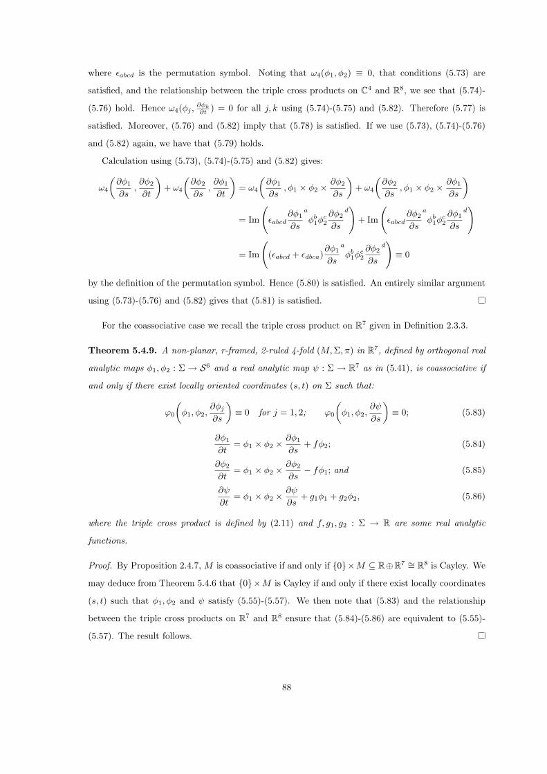
where εabcd is the permutation symbol. Noting that ω4(φ1, φ2) ≡ 0, that conditions (5.73) are
satisfied, and the relationship between the triple cross products on C4 and R8, we see that (5.74)-
(5.76) hold. Hence ω4(φj ,∂φk
∂t ) = 0 for all j, k using (5.74)-(5.75) and (5.82). Therefore (5.77) is
satisfied. Moreover, (5.76) and (5.82) imply that (5.78) is satisfied. If we use (5.73), (5.74)-(5.76)
and (5.82) again, we have that (5.79) holds.
Calculation using (5.73), (5.74)-(5.75) and (5.82) gives:
ω4
(∂φ1
∂s,∂φ2
∂t
)+ ω4
(∂φ2
∂s,∂φ1
∂t
)= ω4
(∂φ1
∂s, φ1 × φ2 × ∂φ2
∂s
)+ ω4
(∂φ2
∂s, φ1 × φ2 × ∂φ1
∂s
)
= Im
(εabcd
∂φ1
∂s
a
φb1φ
c2
∂φ2
∂s
d)
+ Im
(εabcd
∂φ2
∂s
a
φb1φ
c2
∂φ1
∂s
d)
= Im
((εabcd + εdbca)
∂φ1
∂s
a
φb1φ
c2
∂φ2
∂s
d)≡ 0
by the definition of the permutation symbol. Hence (5.80) is satisfied. An entirely similar argument
using (5.73)-(5.76) and (5.82) gives that (5.81) is satisfied.
For the coassociative case we recall the triple cross product on R7 given in Definition 2.3.3.
Theorem 5.4.9. A non-planar, r-framed, 2-ruled 4-fold (M, Σ, π) in R7, defined by orthogonal real
analytic maps φ1, φ2 : Σ → S6 and a real analytic map ψ : Σ → R7 as in (5.41), is coassociative if
and only if there exist locally oriented coordinates (s, t) on Σ such that:
ϕ0
(φ1, φ2,
∂φj
∂s
)≡ 0 for j = 1, 2; ϕ0
(φ1, φ2,
∂ψ
∂s
)≡ 0; (5.83)
∂φ1
∂t= φ1 × φ2 × ∂φ1
∂s+ fφ2; (5.84)
∂φ2
∂t= φ1 × φ2 × ∂φ2
∂s− fφ1; and (5.85)
∂ψ
∂t= φ1 × φ2 × ∂ψ
∂s+ g1φ1 + g2φ2, (5.86)
where the triple cross product is defined by (2.11) and f, g1, g2 : Σ → R are some real analytic
functions.
Proof. By Proposition 2.4.7, M is coassociative if and only if 0×M ⊆ R⊕R7 ∼= R8 is Cayley. We
may deduce from Theorem 5.4.6 that 0×M is Cayley if and only if there exist locally coordinates
(s, t) such that φ1, φ2 and ψ satisfy (5.55)-(5.57). We then note that (5.83) and the relationship
between the triple cross products on R7 and R8 ensure that (5.84)-(5.86) are equivalent to (5.55)-
(5.57). The result follows.
88
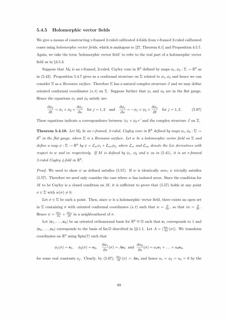
5.4.5 Holomorphic vector fields
We give a means of constructing r-framed 2-ruled calibrated 4-folds from r-framed 2-ruled calibrated
cones using holomorphic vector fields, which is analogous to [27, Theorem 6.1] and Proposition 4.5.7.
Again, we take the term ‘holomorphic vector field’ to refer to the real part of a holomorphic vector
field as in §4.5.3.
Suppose that M0 is an r-framed, 2-ruled, Cayley cone in R8 defined by maps φ1, φ2 : Σ → R8 as
in (5.42). Proposition 5.4.7 gives us a conformal structure on Σ related to φ1, φ2 and hence we can
consider Σ as a Riemann surface. Therefore Σ has a natural complex structure J and we may define
oriented conformal coordinates (s, t) on Σ. Suppose further that φ1 and φ2 are in the flat gauge.
Hence the equations φ1 and φ2 satisfy are:
∂φj
∂t= φ1 × φ2 × ∂φj
∂sfor j = 1, 2 and
∂φj
∂s= −φ1 × φ2 × ∂φj
∂tfor j = 1, 2. (5.87)
These equations indicate a correspondence between ‘φ1 × φ2×’ and the complex structure J on Σ.
Theorem 5.4.10. Let M0 be an r-framed, 2-ruled, Cayley cone in R8 defined by maps φ1, φ2 : Σ →S7 in the flat gauge, where Σ is a Riemann surface. Let w be a holomorphic vector field on Σ and
define a map ψ : Σ → R8 by ψ = Lwφ1 + Liwφ2, where Lw and Liw denote the Lie derivatives with
respect to w and iw respectively. If M is defined by φ1, φ2 and ψ as in (5.41), it is an r-framed
2-ruled Cayley 4-fold in R8.
Proof. We need to show ψ as defined satisfies (5.57). If w is identically zero, ψ trivially satisfies
(5.57). Therefore we need only consider the case where w has isolated zeros. Since the condition for
M to be Cayley is a closed condition on M , it is sufficient to prove that (5.57) holds at any point
σ ∈ Σ with w(σ) 6= 0.
Let σ ∈ Σ be such a point. Then, since w is a holomorphic vector field, there exists an open set
in Σ containing σ with oriented conformal coordinates (s, t) such that w = ∂∂s , so that iw = ∂
∂t .
Hence ψ = ∂φ1∂s + ∂φ2
∂t in a neighbourhood of σ.
Let (e1, . . . , e8) be an oriented orthonormal basis for R8 ∼= O such that e1 corresponds to 1 and
(e2, . . . , e8) corresponds to the basis of ImO described in §2.1.1. Let A = |∂φ1∂s (σ)|. We transform
coordinates on R8 using Spin(7) such that
φ1(σ) = e1, φ2(σ) = e2,∂φ1
∂s(σ) = Ae3 and
∂φ2
∂s(σ) = a1e1 + . . . + a8e8,
for some real constants aj . Clearly, by (5.87), ∂φ1∂t (σ) = Ae4 and hence a1 = a2 = a4 = 0 by the
89

orthogonality conditions imposed on ∂φ2∂s in the flat gauge. Differentiating (5.87) gives:
∂2φ1
∂s∂t= φ1 × ∂φ2
∂s× ∂φ1
∂s+ φ1 × φ2 × ∂2φ1
∂s2and
∂2φ2
∂t2=
∂φ1
∂t× φ2 × ∂φ2
∂s+ φ1 × ∂φ2
∂t× ∂φ2
∂s+ φ1 × φ2 × ∂2φ2
∂t∂s.
Therefore,
∂ψ
∂t=
∂
∂t
(∂φ1
∂s+
∂φ2
∂t
)
= φ1 × ∂φ2
∂s× ∂φ1
∂s+
∂φ1
∂t× φ2 × ∂φ2
∂s+ φ1 × ∂φ2
∂t× ∂φ2
∂s+ φ1 × φ2 × ∂
∂s
(∂φ1
∂s+
∂φ2
∂t
).
Calculation using (2.14) and (5.87) shows that
φ1 × ∂φ2
∂s× ∂φ1
∂s(σ) = A(a7e5 − a8e6 − a5e7 + a6e8),
∂φ1
∂t× φ2 × ∂φ2
∂s(σ) = A(−a3e1 − a7e5 + a8e6 + a5e7 − a6e8) and
φ1 × ∂φ2
∂t× ∂φ2
∂s(σ) = −(a2
3 + a25 + a2
6 + a27 + a2
8)e2.
We conclude that (5.57) holds for ψ at σ with g1(σ) = −Aa3 = −g0
(∂φ1∂s (σ) , ∂φ2
∂s (σ))
and g2(σ) =
−|∂φ2∂s (σ)|2. By the invariance of g0 and the triple cross product under Spin(7), and the discussion
above, ψ satisfies (5.57) for some g1, g2 : Σ → R. Applying Theorem 5.4.6, the proof is complete.
This result does not generalise to the SL case in the way we might expect. The construction
starting with a 2-ruled SL cone M0 will generally produce a 2-ruled Cayley, but not SL, 4-fold M .
The fact that M is Cayley follows trivially from Theorem 5.4.10, but if we impose the condition
ω4|M ≡ 0, φ1 and φ2 must also satisfy
ω4
(∂φ1
∂s,∂φ2
∂s
)= −ω4
(∂φ1
∂t,∂φ2
∂t
)= 0 and ω4
(∂φ1
∂s,∂φ2
∂t
)= ω4
(∂φ1
∂t,∂φ2
∂s
)= 0
wherever w 6= 0. At such a point, either all the derivatives of φ1 and φ2 are zero or at least one is
nonzero. In the first case both φ1 and φ2 are locally constant. Otherwise, suppose without loss of
generality that ∂φ1∂s 6= 0 at a point σ such that w(σ) 6= 0. Then 〈∂φ1
∂s , ∂φ1∂t 〉C = C2 and it is orthogonal
to 〈φ1, φ2〉C = C2 since M is SL and φ1, φ2 are in the flat gauge. Therefore ∂φ2∂s ∈ 〈∂φ1
∂s , ∂φ1∂t 〉C. Note
that g4(∂φ1∂t , ∂φ2
∂s ) = ω4(∂φ1∂t , ∂φ2
∂s ) = 0 and ω4(∂φ1∂s , ∂φ2
∂s ) = 0. Hence there exists θ ∈ R such that
cos θ ∂φ1∂s +sin θ ∂φ2
∂s = 0. Using (5.87), cos θ ∂φ1∂t +sin θ ∂φ2
∂t = 0. Therefore, cos θφ1+sin θφ2 is constant
on a neighbourhood of σ and thus on the component of Σ containing σ. We deduce the following.
Theorem 5.4.11. Let M0 be an r-framed, 2-ruled, SL cone in C4 ∼= R8 defined by φ1, φ2 : Σ → S7
in the flat gauge, where Σ is a Riemann surface. Let w be a holomorphic vector field on Σ and
define ψ : Σ → C4 by ψ = Lwφ1 +Liwφ2, where Lw and Liw denote the Lie derivatives with respect
90
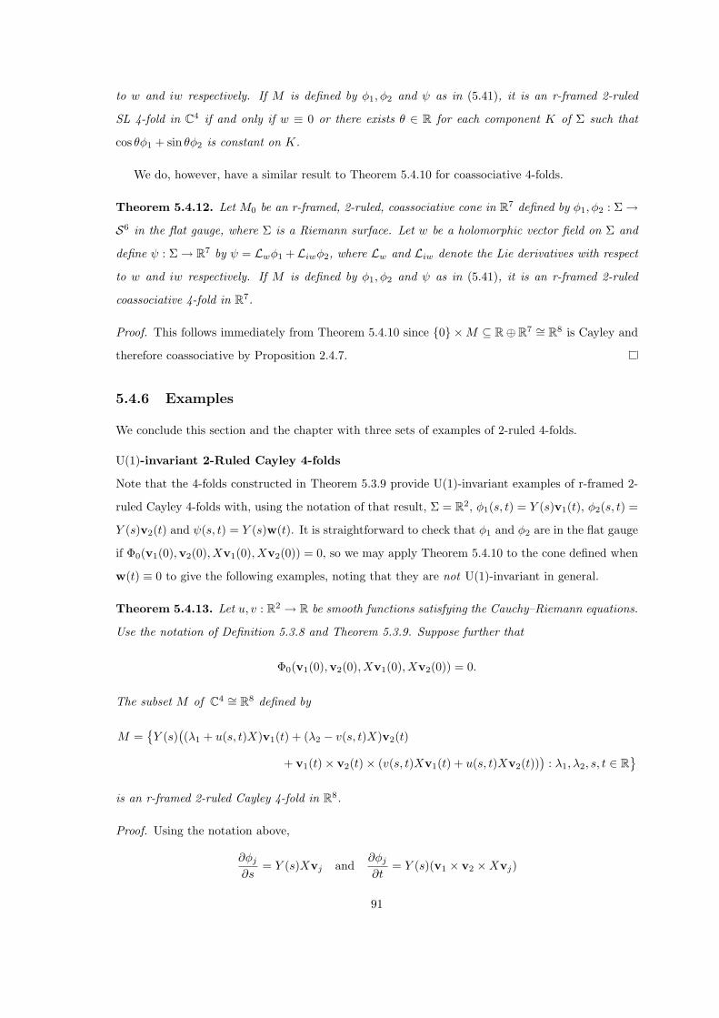
to w and iw respectively. If M is defined by φ1, φ2 and ψ as in (5.41), it is an r-framed 2-ruled
SL 4-fold in C4 if and only if w ≡ 0 or there exists θ ∈ R for each component K of Σ such that
cos θφ1 + sin θφ2 is constant on K.
We do, however, have a similar result to Theorem 5.4.10 for coassociative 4-folds.
Theorem 5.4.12. Let M0 be an r-framed, 2-ruled, coassociative cone in R7 defined by φ1, φ2 : Σ →S6 in the flat gauge, where Σ is a Riemann surface. Let w be a holomorphic vector field on Σ and
define ψ : Σ → R7 by ψ = Lwφ1 +Liwφ2, where Lw and Liw denote the Lie derivatives with respect
to w and iw respectively. If M is defined by φ1, φ2 and ψ as in (5.41), it is an r-framed 2-ruled
coassociative 4-fold in R7.
Proof. This follows immediately from Theorem 5.4.10 since 0 ×M ⊆ R⊕ R7 ∼= R8 is Cayley and
therefore coassociative by Proposition 2.4.7.
5.4.6 Examples
We conclude this section and the chapter with three sets of examples of 2-ruled 4-folds.
U(1)-invariant 2-Ruled Cayley 4-folds
Note that the 4-folds constructed in Theorem 5.3.9 provide U(1)-invariant examples of r-framed 2-
ruled Cayley 4-folds with, using the notation of that result, Σ = R2, φ1(s, t) = Y (s)v1(t), φ2(s, t) =
Y (s)v2(t) and ψ(s, t) = Y (s)w(t). It is straightforward to check that φ1 and φ2 are in the flat gauge
if Φ0(v1(0),v2(0), Xv1(0), Xv2(0)) = 0, so we may apply Theorem 5.4.10 to the cone defined when
w(t) ≡ 0 to give the following examples, noting that they are not U(1)-invariant in general.
Theorem 5.4.13. Let u, v : R2 → R be smooth functions satisfying the Cauchy–Riemann equations.
Use the notation of Definition 5.3.8 and Theorem 5.3.9. Suppose further that
Φ0(v1(0),v2(0), Xv1(0), Xv2(0)) = 0.
The subset M of C4 ∼= R8 defined by
M =Y (s)
((λ1 + u(s, t)X)v1(t) + (λ2 − v(s, t)X)v2(t)
+ v1(t)× v2(t)× (v(s, t)Xv1(t) + u(s, t)Xv2(t)))
: λ1, λ2, s, t ∈ R
is an r-framed 2-ruled Cayley 4-fold in R8.
Proof. Using the notation above,
∂φj
∂s= Y (s)Xvj and
∂φj
∂t= Y (s)(v1 × v2 ×Xvj)
91

for j = 1, 2. Further, we may write a holomorphic vector field w, and hence iw, on R2 as:
w = u(s, t)∂
∂s+ v(s, t)
∂
∂tand iw = −v(s, t)
∂
∂s+ u(s, t)
∂
∂t.
The result follows from Theorem 5.4.10.
Now consider the family of SL 4-folds in C4 given in [17, Theorem III.3.1]. Let c = (c1, c2, c3, c4)
in R4 be constant and define Mc ⊆ C4 by:
Mc = (z1, z2, z3, z4) ∈ C4 : Re(z1z2z3z4) = c1 and |z1|2 − |zj |2 = cj for j = 2, 3, 4.
Then Mc is an SL 4-fold in C4 invariant under U(1)3.
Taking c = 0, M0 is an r-framed 2-ruled SL cone in C4 with three different 2-rulings. For each
of the distinct 2-rulings we apply the holomorphic vector field result of Theorem 5.4.11 to obtain
families of r-framed 2-ruled Cayley 4-folds which are invariant under U(1).
Theorem 5.4.14. Let w : C→ C be a holomorphic function. Then
M1 =
12
(ieis
(reiθ+ iw(s + it)
), e−is
(reiθ− iw(s + it)
),
eit(re−iθ+ w(s + it)
), e−it
(re−iθ− w(s + it)
) ): r, s, t, θ ∈ R
,
M2 =
12
(ieis
(reiθ+ iw(s + it)
), e−it
(re−iθ− w(s + it)
),
eit(re−iθ+ w(s + it)
), e−is
(reiθ− iw(s + it)
) ): r, s, t, θ ∈ R
and
M3 =
12
(ieis
(reiθ+ iw(s + it)
), eit
(re−iθ+ w(s + it)
),
e−is(reiθ− iw(s + it)
), e−it
(re−iθ− w(s + it)
) ): r, s, t, θ ∈ R
are r-framed 2-ruled Cayley 4-folds in R8 ∼= C4.
Proof. We only prove the result for M1 as the proof for the other two is similar. In this example we
define M0 by functions φ1, φ2 : R2 → S7 ⊆ C4 given by:
φ1(s, t) =12(ieis, e−is, eit, e−it) and φ2(s, t) =
i
2(ieis, e−is,−eit,−e−it).
Thus, M0 is 2-ruled by planes of the form:
Πr, θ = r cos θ φ1(s, t) + r sin θ φ2(s, t) : s, t ∈ R
=r
2
(iei(θ+s), ei(θ−s), e−i(θ−t), e−i(θ+t)
): s, t ∈ R
.
We verify through direct calculation that g4(φ1, φ2) = ω4(φ1, φ2) = 0, the first equation in (5.73)
holds, (5.74)-(5.75) with f = 0 are satisfied, and that φ1 and φ2 are in the flat gauge.
92
Let w(s + it) = u(s, t) + iv(s, t) for functions u, v : R2 → R. Then ψ = Lwφ1 + Liwφ2 is:
ψ(s, t) = u(s, t)∂φ1
∂s+ v(s, t)
∂φ1
∂t− v(s, t)
∂φ2
∂s+ u(s, t)
∂φ2
∂t
=12
(iw(s + it)ieis,−iw(s + it)e−is, w(s + it)eit,−w(s + it)e−it
).
We check that ψ satisfies (5.57) with g1 = 0 and g2 = − 12 , which agrees with the calculations in the
proof of Theorem 5.4.10. Therefore, by Theorem 5.4.10, M1 is an r-framed 2-ruled Cayley 4-fold.
Note, from the proof above, that 2ω4(φ1,∂ψ∂s ) = v and 2ω4(φ1,
∂ψ∂s ) = u, so that (5.73) of Theorem
5.4.8 is satisfied if and only if w ≡ 0. Therefore, if w is not zero, Theorem 5.4.11 shows that M1 is
an r-framed 2-ruled Cayley 4-fold which is not SL. Similarly for M2 and M3.
An interesting special case is when w in Theorem 5.4.14 is taken to be constant. Here, calculation
shows that, each Mj is invariant under a U(1)2 subgroup of U(1)3. Moreover, they are asymptotically
conical to M0 with rate −1, in the sense of Definition 1.2.3.
1-Ruled Associative and Special Lagrangian 3-folds
We can construct examples of 2-ruled 4-folds from 1-ruled associative 3-folds in R7 and SL 3-folds
in C3, as described in §4.5 and [27] respectively. Recall the notation of Definition 4.5.1.
Suppose that (N, Σ, π) is a 1-ruled 3-fold. Let M = R × N and let π : M → Σ be given by
π(r, p) = π(p) for all p ∈ N . Clearly, (M, Σ, π) is a 2-ruled 4-fold since π−1(σ) = R × π−1(σ) for
all σ ∈ Σ. Suppose further that (N, Σ, π) is r-oriented. Using the r-orientation, we have a natural
choice of oriented orthonormal basis for the plane π−1(σ), which varies smoothly with σ. Therefore,
(M, Σ, π) is r-framed.
We now state and prove the following theorem.
Theorem 5.4.15. (a) If N ⊆ R7 is an (r-oriented) 1-ruled associative 3-fold, R×N ⊆ R⊕R7 ∼=R8 is an (r-framed) 2-ruled Cayley 4-fold.
(b) If L ⊆ C3 is an (r-oriented) 1-ruled SL 3-fold with phase −i, R × L ⊆ R ⊕ C3 ∼= R7 is an
(r-framed) 2-ruled coassociative 4-fold.
Proof. Let N be an associative 3-fold in R7. By Proposition 2.4.7, R×N is Cayley. The comments
before the theorem then give the result (a). Similarly, (b) follows from Proposition 3.1.3 and the
comments above.
Complex Cones
Define a complex cone C in C4 by:
C = (z1, z2, z3, z4) ∈ C4 : P (z1, z2, z3, z4) = Q(z1, z2, z3, z4) = 0,
93

where P and Q are homogeneous complex polynomials such that C is non-planar and nonsingular
except at 0. Define a projection π from C \ 0 to CP3 by π((z1, z2, z3, z4)) = [(z1, z2, z3, z4)] and let
Σ be the image of π. Let
M0 = (z1, z2, z3, z4, σ) ∈ C × Σ : (z1, z2, z3, z4) ∈ σ
and define ι : M0 → C4 by ι(z1, z2, z3, z4, σ) = (z1, z2, z3, z4). Then ι is an immersion except at 0
and thus M0 is an immersed submanifold of C4 which is only singular at 0. Let π : M0 → Σ be
given by π(z1, z2, z3, z4, σ) = σ. Clearly, M0 is 2-ruled by complex lines π−1(σ) in C4. Since any
complex surface in C4 ∼= R8 is Cayley by [17, §IV.2.C], (M0,Σ, π) is a 2-ruled Cayley 4-fold.
We can define a local holomorphic coordinate w, hence oriented conformal coordinates (s, t), in
Σ by w 7→ [(z1, z2, z3, z4)](w) in some open set U in Σ. Suppose without loss of generality that
z4 6= 0 in U . Then, we may rescale so that z4 = 1 and define maps φ1, φ2 : U → S7 by:
φ1(s, t) =(
z1(s, t)r
,z2(s, t)
r,z3(s, t)
r,1r
)and φ2(s, t) = iφ1(s, t),
where r = (1+ |z1(s, t)|2 + |z2(s, t)|2 + |z3(s, t)|2) 12 . We can thus write M0 locally in the form (5.42),
where φ1 and φ2 satisfy (5.55)-(5.56), since C and hence M0 is non-planar. If we define M by (5.41)
where ψ satisfies (5.57) then, from Theorem 5.4.6, M is a non-planar, r-framed, 2-ruled Cayley 4-fold
in R8.
94

Part II
Noncompact Coassociative
Deformations
Abstractness, sometimes hurled as a reproach at mathematics, is its chief glory and its
surest title to practical usefulness. It is also the source of such beauty as may spring
from mathematics.– Eric Temple Bell
95
Chapter 6
Analysis on Noncompact
Riemannian Manifolds
Various analytic techniques may be employed on certain classes of noncompact Riemannian manifold.
A key idea, presented in §6.2, is the introduction of weighted versions of Sobolev and Holder spaces.
This enables the study of Fredholm and index theory of uniformly elliptic operators between these
Banach spaces in §6.3 and the description of elliptic regularity results in §6.4.
6.1 AC and CS Manifolds
We are interested in two types of noncompact Riemannian manifolds: asymptotically conical mani-
folds and manifolds with conical singularities.
Definition 6.1.1. Let (M, g) be a Riemannian manifold with dim M = n. Then M is asymptotically
conical (AC) (with rate λ) if there exist constants R > 0 and λ < 1, a compact (n−1)-dimensional
Riemannian manifold (Σ, h), a compact set K ⊆ M and a diffeomorphism Ψ : (R,∞)×Σ → M \K
such that
|∇j(Ψ∗(g)− g cone)| = O(rλ−1−j) for j ∈ N as r →∞, (6.1)
where r is the coordinate on (0,∞) on the cone C = (0,∞) × Σ, g cone = dr2 + r2h is the conical
metric on C, ∇ is the Levi–Civita connection derived from g cone and |.| is calculated using gcone.
We call C the asymptotic cone of M and define the ends M∞ of M to be the components of M \K.
The choice of λ < 1 ensures that the metric on M converges to the conical metric on C at infinity
by (6.1). It is also clear, from Definition 1.2.3, that a Riemannian submanifold of Rn which is AC
with rate λ to a cone M0 is an AC Riemannian manifold with rate λ, where Σ = M0 ∩ Sn−1.
96

Definition 6.1.2. Let M be an AC manifold and use the notation of Definition 6.1.1. A radius
function ρ : M → [1,∞) on M is a smooth function such that there exist positive constants c1 < 1
and c2 > 1 with c1r < Ψ∗(ρ) < c2r on (R,∞)× Σ.
If M is AC we may define a radius function ρ : M → [1,∞) on it using r, by requiring that ρ is
equal to r on Ψ((R + 1,∞)× Σ) and then extending ρ smoothly to a function on M .
Definition 6.1.3. Let M be a connected Hausdorff topological space and let z1, . . . , zs ∈ M .
Suppose that M = M \ z1, . . . , zs has the structure of a (nonsingular) n-dimensional Riemannian
manifold, with Riemannian metric g, compatible with its topology. Then M is a manifold with
conical singularities (at z1, . . . , zs with rate λ) if there exist constants ε > 0 and λ > 1, a compact
(n−1)-dimensional Riemannian manifold (Σi, hi), an open set Ui 3 zi in M with Ui ∩ Uj = ∅ for
j 6= i and a diffeomorphism Ψi : (0, ε)× Σi → Ui \ zi ⊆ M , for i = 1, . . . , s, such that
|∇ji (Ψ
∗i (g)− gi)| = O(rλ−1−j
i ) for j ∈ N as ri → 0, (6.2)
where ri is the coordinate on (0,∞) on the cone Ci = (0,∞) × Σi, gi = dr2i + r2
i hi is the conical
metric on Ci, ∇i is the Levi–Civita connection derived from gi and |.| is calculated using gi. We call
Ci the cone at the singularity zi and let the ends M∞ of M be the disjoint union
M∞ =s⊔
i=1
Ui \ zi.
We say that M is CS or a CS manifold (with rate λ) if it is a manifold with conical singularities
which have rate λ and it is compact as a topological space. In these circumstances it may be written
as the disjoint union
M = K ts⊔
i=1
Ui,
where K is compact as it is closed in M .
The condition λ > 1 guarantees that the metric on M genuinely converges to the conical metric
on Ci, as is evident from (6.2). Since M is supposed to be Hausdorff, the set Ui \ zi is open in
M for all i. Moreover, the condition that the Ui are disjoint may be easily satisfied since, if i 6= j,
zi and zj may be separated by two disjoint open sets and, by hypothesis, there are only a finite
number of singularities.
It is also important to note that M is a noncompact manifold.
Definition 6.1.4. Let M be a CS manifold. Using the notation of Definition 6.1.3, a radius function
on M is a smooth function ρ : M → (0, 1], bounded below by a positive constant on M \ M∞, such
that there exist positive constants c1 < 1 and c2 > 1 with
c1ri < Ψ∗i (ρ) < c2ri
97

on (0, ε)× Σi for i = 1, . . . , s.
If M is CS we may construct a radius function on M as follows. Let ρ(x) = 1 for all x ∈M \ M∞. Define ρi : Ψi((0, ε/2) × Σi) → (0, 1) to be equal to ri for i = 1, . . . , s and then define
ρ by interpolating smoothly between its definition on M \ M∞ and ρi on each of the disjoint sets
Ψi((ε/2, ε)× Σi).
For the purposes of this chapter only, we shall henceforth, when referring to a CS manifold, mean
the nonsingular part M of M , in the notation of Definition 6.1.3.
6.2 Weighted Banach Spaces
We define weighted Banach spaces of forms as in [3, §1], as well as the usual ‘unweighted’ spaces.
Definition 6.2.1. Let (M, g) be a Riemannian n-fold, let p ≥ 1 and let k, m ∈ N with m ≤ n. The
Sobolev space Lpk(ΛmT ∗M) is the set of m-forms ξ on M which are k times weakly differentiable
and such that the norm
‖ξ‖Lpk
=
k∑
j=0
∫
M
|∇jξ|p dVg
1p
(6.3)
is finite. The normed vector space Lpk(ΛmT ∗M) is a Banach space for all p ≥ 1 and L2
k(ΛmT ∗M) is
a Hilbert space.
We introduce the space of m-forms
Lpk, loc(Λ
mT ∗M) = ξ : fξ ∈ Lpk(ΛmT ∗M) for all f ∈ C∞cs (M)
where C∞cs (M) is the space of smooth functions on M with compact support.
Suppose further that M is AC or CS. Let µ ∈ R and let ρ be a radius function on M . The
weighted Sobolev space Lpk, µ(ΛmT ∗M) of m-forms ξ on M is the subspace of Lp
k, loc(ΛmT ∗M) such
that the norm
‖ξ‖Lpk, µ
=
k∑
j=0
∫
M
|ρj−µ∇jξ|pρ−n dVg
1p
(6.4)
is finite. Then Lpk, µ(ΛmT ∗M) is a Banach space and L2
k, µ(ΛmT ∗M) is a Hilbert space.
We may note here, trivially, that Lp0(Λ
mT ∗M) is equal to the standard Lp-space of m-forms
on M . Further, by comparing equations (6.3) and (6.4) for the respective norms, Lp(ΛmT ∗M) =
Lp0,−n
p(ΛmT ∗M). In particular,
L2(ΛmT ∗M) = L20,−n
2(ΛmT ∗M). (6.5)
98

For the following two definitions we take Ckloc(Λ
mT ∗M) to be the vector space of k times con-
tinuously differentiable m-forms.
Definition 6.2.2. Let (M, g) be an n-dimensional AC or CS manifold and let ρ be a radius function
on M . Let µ ∈ R and let k,m ∈ N with m ≤ n. The weighted Ck-space Ckµ(ΛmT ∗M) of m-forms ξ
on M is the subspace of Ckloc(Λ
mT ∗M) such that the norm
‖ξ‖Ckµ
=k∑
j=0
supM|ρj−µ∇jξ|
is finite. We also define
C∞µ (ΛmT ∗M) =⋂
k≥0
Ckµ(ΛmT ∗M).
Then Ckµ(ΛmT ∗M) is a Banach space but in general C∞µ (ΛmT ∗M) is not.
In the next definition we refer to the usual normed vector space Ck(ΛmT ∗M) of k times contin-
uously differentiable m-forms such that the following norm is finite:
‖ξ‖Ck =k∑
j=0
supM|∇jξ|.
Definition 6.2.3. Let (M, g) be an n-dimensional AC or CS manifold, let d(x, y) be the geodesic
distance between points x, y ∈ M and let ρ be a radius function on M . Let a ∈ (0, 1) and let
k, m ∈ N with m ≤ n. Let
H = (x, y) ∈ M ×M : x 6= y, c1ρ(x) ≤ ρ(y) ≤ c2ρ(x) and
there exists a geodesic in M of length d(x, y) from x to y,
where 0 < c1 < 1 < c2 are constant. A section s of a vector bundle V on M is Holder continuous
(with exponent a) if
[s]a = sup(x,y)∈H
|s(x)− s(y)|Vd(x, y)a
< ∞.
We understand the quantity |s(x)− s(y)|V as follows. Given (x, y) ∈ H, there exists a geodesic γ of
length d(x, y) connecting x and y. Parallel translation along γ using the connection on V identifies
the fibres over x and y and the metrics on them. Thus, with this identification, |s(x) − s(y)|V is
well-defined.
The Holder space Ck, a(ΛmT ∗M) is the set of ξ ∈ Ck(ΛmT ∗M) such that ∇kξ is Holder contin-
uous (with exponent a) and the norm
‖ξ‖Ck, a = ‖ξ‖Ck + [∇kξ]a
is finite. The normed vector space Ck, a(ΛmT ∗M) is a Banach space.
99
We also introduce the notation
Ck, aloc (ΛmT ∗M) =ξ ∈ Ck
loc(ΛmT ∗M) : fξ ∈ Ck, a(ΛmT ∗M) for all f ∈ C∞cs (M).
Let µ ∈ R. The weighted Holder space Ck, aµ (ΛmT ∗M) of m-forms ξ on M is the subspace of
Ck, aloc (ΛmT ∗M) such that the norm
‖ξ‖Ck, aµ
= ‖ξ‖Ckµ
+ [ξ]k, aµ
is finite, where
[ξ]k, aµ = [ρk+a−µ∇kξ]a.
Then Ck, aµ (ΛmT ∗M) is a Banach space. It is clear that we have an embedding Ck, a
µ (ΛmT ∗M) →Cl
µ(ΛmT ∗M) whenever l ≤ k.
We shall need the analogue of the Sobolev Embedding Theorem for weighted spaces, which is
adapted from [37, Lemma 7.2] and [3, Theorem 1.2]. It is dependent on whether M is AC or CS.
Theorem 6.2.4 (Weighted Sobolev Embedding Theorem). Let M be an n-dimensional AC
(or CS) manifold. Let p, q ≥ 1, a ∈ (0, 1), µ, ν ∈ R and k, l,m ∈ N with m ≤ n.
(a) If k ≥ l, k − np ≥ l − n
q and either
(i) p ≤ q and µ ≤ ν if M is AC (or µ ≥ ν if M is CS) or
(ii) p > q and µ < ν if M is AC (or µ > ν if M is CS),
there is a continuous embedding Lpk, µ(ΛmT ∗M) → Lq
l, ν(ΛmT ∗M).
(b) If k − np ≥ l + a, there is a continuous embedding Lp
k, µ(ΛmT ∗M) → Cl, aµ (ΛmT ∗M).
We shall also require an Implicit Function Theorem for Banach spaces, which follows immediately
from [34, Chapter 6, Theorem 2.1].
Theorem 6.2.5 (Implicit Function Theorem). Let X and Y be Banach spaces and let W ⊆ X
be an open neighbourhood of 0. Let G : W → Y be a Ck map (k ≥ 1) such that G(0) = 0. Suppose
further that dG|0 : X → Y is surjective with kernel K such that X = K⊕A for some closed subspace
A of X. There exist open sets V ⊆ K and V ′ ⊆ A, both containing 0, with V × V ′ ⊆ W , and a
unique Ck map V : V → V ′ such that
KerG ∩ (V × V ′) = (x,V(x)) : x ∈ V
in X = K ⊕A.
100

6.3 Uniformly Elliptic AC and CS Operators
We must begin by defining the operators that we shall be concerned with.
Definition 6.3.1. Let V and W be bundles of forms over an AC or CS manifold M , let l ∈ N,
let ν ∈ R and let P be a linear differential operator of order l from V to W . Use the notation of
Definitions 6.1.1 and 6.1.3. Transform coordinates (r, σ) on the ends of M to cylindrical coordinates
(t, σ); that is, r = Ret in the AC case and r = εe−t in the CS case. Let P ν = eνtP be the
operator on the cylindrical ends (0,∞) × Σ of M , where we take Σ = tsi=1Σi for the CS case. Let
π : (0,∞) × Σ → Σ be the projection map and let VΣ and WΣ be the bundles of forms over Σ
such that V∞ = π∗(VΣ) and W∞ = π∗(WΣ) are bundles over the ends corresponding to V and W
respectively. Write
P νξ =l∑
i=0
P νi ∇iξ
for ξ ∈ Clloc(V∞), where the P ν
i are tensors taking values in V ∗∞ ⊗ W∞ and ∇ is the Levi–Civita
connection of the cylindrical metric. We say that P ν is asymptotically cylindrical if there exists a
linear differential operator P∞ of order l from V∞ to W∞, which may be written as
P∞ξ =l∑
i=0
Pi,∞∇iξ,
such that Pi,∞ is translation invariant on the ends of M in cylindrical coordinates and
|∇j(P νi − Pi,∞)| → 0 for j ∈ N as t →∞
for all i. If P ν is asymptotically cylindrical then P is AC or CS with rate ν as appropriate.
Note that an AC or CS operator with rate ν reduces the growth rate of a form on the ends of M by
ν. Examples of AC or CS operators abound: d and d∗ are first order operators with rate 1 and the
Laplacian is a second order operator with rate 2.
Definition 6.3.2. Use the notation of Definition 6.3.1. We say that an AC or CS operator P is
uniformly elliptic if it is elliptic and P∞ is elliptic.
We observe that the definition of uniformly elliptic above implies uniform ellipticity in the sense of
global bounds on the coefficients of the symbol. The operators d+d∗ and the Laplacian are examples
of uniformly elliptic operators.
6.3.1 Fredholm theory
We have a general Fredholm result adapted from [37, Theorem 1.1 & Theorem 6.1].
101

Theorem 6.3.3. Let V and W be bundles of forms over an AC or CS manifold M , let p ≥ 1, let
µ, ν ∈ R, let k, l ∈ N and let P : Lpk+l, µ(V ) → Lp
k, µ−ν(W ) be a uniformly elliptic AC or CS operator,
respectively, of order l and rate ν. There exists a countable discrete set D(P ) ⊆ R, depending only
on P∞ as in Definition 6.3.1, such that P is Fredholm if and only if µ /∈ D(P ).
We shall be primarily concerned with the uniformly elliptic map
d + d∗ : Lpk+1, µ(Λ2
+T ∗M ⊕ Λ4T ∗M) → Lpk, µ−1(Λ
3T ∗M), (6.6)
where M is 4-dimensional. We give an explicit description of the set DAC for which (6.6) is not
Fredholm in the AC case, following [42, §6.1.2].
Recall the notation of Definition 6.1.1. Transform the asymptotically conical metric on M to a
conformally equivalent asymptotically cylindrical metric; that is, if (t, σ) are coordinates on (0,∞)×Σ, the metric is asymptotic to dt2 + gΣ. With respect to this new metric, d + d∗ corresponds to
(d + d∗)∞ = e−mt(d + e2td∗)emt
acting on m-forms on M . If π : (0,∞)×Σ → Σ is the natural projection map, the action of (d+d∗)∞
on π∗(Λ2T ∗Σ)⊕ π∗(ΛoddT ∗Σ) is:
(d + d∗)∞ =
d + d∗ −( ∂
∂t + 3−m)
∂∂t + m −(d + d∗)
(6.7)
where m denotes the operator which multiplies m-forms by a factor m. However, we wish only to
consider elements of Λ1T ∗Σ ⊕ Λ2T ∗Σ which correspond to self-dual 2-forms on M , so we define
VΣ ⊆ Λ2T ∗Σ⊕ ΛoddT ∗Σ by
VΣ = (α, ∗α + β) : α ∈ Λ2T ∗Σ, β ∈ Λ3T ∗Σ.
Then π∗(VΣ) corresponds to Λ2+T ∗M ⊕ Λ4T ∗M .
For w ∈ C define a map (d + d∗)∞(w) by:
(d + d∗)∞(w) =
d + d∗ −(w + 3−m)
w + m −(d + d∗)
(6.8)
acting on VΣ ⊗ C. Notice that we have formally substituted w for ∂∂t in (6.7).
Let
WΣ = (∗α + β, α) : α ∈ Λ2T ∗Σ, β ∈ Λ3T ∗Σ ⊆ ΛoddT ∗Σ⊕ Λ2T ∗Σ.
Define C ⊆ C as the set of w for which the map
(d + d∗)∞(w) : Lpk+1(VΣ ⊗ C) → Lp
k(WΣ ⊗ C)
102

is not an isomorphism. By the proof of [37, Theorem 1.1], DAC = Re w : w ∈ C. In fact, C ⊆ R by
[42, Lemma 6.1.13], which shows that the corresponding sets C(∆m) are all real, where ∆m is the
Laplacian on m-forms. Hence C = DAC.
The symbol, hence the index indw, of (d + d∗)∞(w) is independent of w. Furthermore, (d +
d∗)∞(w) is an isomorphism for generic values of w since DAC is countable and discrete. Therefore
indw = 0 for all w ∈ C; that is,
dim Ker(d + d∗)∞(w) = dim Coker(d + d∗)∞(w),
so that (6.8) is not an isomorphism precisely when it is not injective.
The condition (d + d∗)∞(w) = 0, using (6.8), corresponds to the existence of α ∈ C∞(Λ2T ∗Σ)
and β ∈ C∞(Λ3T ∗Σ) satisfying
dα = wβ and d∗α + d∗β = (w + 2)α. (6.9)
We first note that (6.9) implies that
dd∗β = ∆β = w(w + 2)β.
Since eigenvalues of the Laplacian on Σ must necessarily be positive, β = 0 if w ∈ (−2, 0). If w = 0
and we take α = 0, (6.9) forces β to be coclosed. As there are non-trivial coclosed 3-forms on Σ,
(d + d∗)∞(0) is not injective and hence 0 ∈ DAC.
Suppose that w = −2 lies in DAC. Then (6.9) gives [β] = 0 in H3dR(Σ). We know that β is
harmonic so, by Hodge theory, β = 0. Therefore −2 ∈ DAC if and only if there exists a nonzero
closed and coclosed 2-form on Σ.
We state a proposition which follows from the work above noting that, with minor adjustment,
the same arguments will apply to the CS case.
Proposition 6.3.4. (a) Let M be a 4-dimensional AC manifold. Use the notation of Definition
6.1.1. Let D(µ) = (α, β) ∈ C∞(Λ2T ∗Σ⊕ Λ3T ∗Σ) : dα = µβ, d∗α + d∗β = (µ + 2)α. The
set DAC of real numbers µ for which (6.6) is not Fredholm is given by:
DAC = µ ∈ R : D(µ) 6= 0.
(b) Let M be a 4-dimensional CS manifold. Use the notation of Definition 6.1.3. For i = 1, . . . , s
let D(µ, i) = (α, β) ∈ C∞(Λ2T ∗Σi ⊕ Λ3T ∗Σi) : dα = µβ, d∗α + d∗β = (µ − 2)α. The set
DCS of real numbers µ such that (6.6) is not Fredholm is given by:
DCS =s⋃
i=1
µ ∈ R : D(µ, i) 6= 0.
103

A perhaps more illuminating way to characterise D(µ) and D(µ, i) is by:
(α, β) ∈ D(µ) ⇐⇒ ξ = (rµ+2α + rµ+1dr ∧ ∗α, rµ+3dr ∧ β)
is an O(rµ) solution of (d + d∗)ξ = 0 on C and
(α, β) ∈ D(µ, i) ⇐⇒ ξ = (rµ−2α + rµ−1dr ∧ ∗α, rµ−3dr ∧ β)
is an O(rµ) solution of (d + d∗)ξ = 0 on Ci,
using the notation of Definitions 6.1.1 and 6.1.3.
6.3.2 Index theory
We begin with some definitions following [37].
Definition 6.3.5. Use the notation of Definition 6.3.1 and Theorem 6.3.3. Let µ ∈ D(P ). Define
d(µ) to be the dimension of the vector space of solutions of P∞ξ = 0 of the form
ξ(t, σ) = eµtp (t, σ)
where p (t, σ) is a polynomial in t ∈ (0,∞) with coefficients in C∞(VΣ ⊗ C). We also define, for
λ, λ′ /∈ D(P ) with λ′ ≤ λ, the quantity
N(λ, λ′) =∑
µ∈D(P )∩(λ′, λ)
d(µ).
The next result is immediate from [37, Theorem 1.2].
Theorem 6.3.6. Use the notation of Theorem 6.3.3. Let λ, λ′ /∈ D(P ) with λ′ ≤ λ. For any
µ /∈ D(P ) let indµ(P ) denote the Fredholm index of P : Lpk+l, µ(V ) → Lp
k, µ−ν(W ). If M is AC,
indλ(P )− indλ′(P ) = N(λ, λ′).
If M is CS,
indλ′(P )− indλ(P ) = N(λ, λ′).
We make a key observation, which shall be used on a number of occasions in Chapters 7 and 8.
Proposition 6.3.7. Use the notation of Theorem 6.3.3. Let λ, λ′ ∈ R such that λ′ ≤ λ and
[λ′, λ] ∩ D(P ) = ∅. The kernels, and cokernels, of P : Lpk+l, µ(V ) → Lp
k, µ−ν(W ) when µ = λ and
µ = λ′ are equal.
Proof. Denote the dimensions of the kernel and cokernel of P : Lpk+l, µ(V ) → Lp
k, µ−ν(W ), for
µ /∈ D(P ), by k(µ) and c(µ) respectively. Since [λ′, λ] ∩ D(P ) = ∅, k(λ)− c(λ) = k(λ′)− c(λ′) and
hence
k(λ)− k(λ′) = c(λ)− c(λ′). (6.10)
104

Suppose that M is an n-dimensional AC manifold. We therefore know that k(λ) ≥ k(λ′) because
Lpk+1, λ′ → Lp
k+1, λ by Theorem 6.2.4(a) as λ ≥ λ′. Similarly, since c(µ) is equal to the dimension
of the kernel of the formal adjoint operator acting on a Sobolev space with weight −n − (µ − ν),
c(λ) ≤ c(λ′). Noting that the left-hand side of (6.10) is non-negative and the right-hand side is less
than or equal to zero, we conclude that both must be zero. The result for the AC case follows from
the fact that the kernel of P in Lpk+1, λ′ is contained in the kernel of P in Lp
k+1, λ, and vice versa for
the cokernels.
If M is a CS manifold, we need only note that the direction of embeddings of Sobolev spaces
is reversed from the AC scenario, so that the signs of each side of (6.10) are swapped. The same
deductions as above may thus be made and the proposition is proved.
We now go further and give a more explicit description of the quantity d(µ) in Definition 6.3.5
for the set DAC given in Proposition 6.3.4. We assume M is AC, but a similar argument will hold
if M is CS.
Use the notation of Proposition 6.3.4 and the work preceding it and Definition 6.3.5. Let p(t, σ)
be a polynomial in t of degree m written as
p(t, σ) =m∑
j=0
pjtj +
m∑
j=0
(∗pj + qj)tj ,
where pj ∈ C∞(Λ2T ∗Σ) and qj ∈ C∞(Λ3T ∗Σ) for j = 0, . . . , m, with pm and qm not both zero, and
let ξ(t, σ) = eµtp(t, σ). Using (6.7), (d + d∗)∞ξ = 0 is equivalent tom∑
j=0
tj(dpj − µqj)−m∑
j=0
jtj−1qj = 0 andm∑
j=0
tj((µ + 2)pj − d∗pj − d∗qj) +m∑
j=0
jtj−1pj = 0.
(6.11)
Comparing coefficients of tm we deduce that (pm, qm) ∈ D(µ). We know for µ ∈ DAC that D(µ) 6= 0,
so we may take m = 0.
Suppose that m ≥ 1. Comparing coefficients of tm−1 in (6.11):
dpm−1 − µqm−1 = mqm and d∗pm−1 + d∗qm−1 − (µ + 2)pm−1 = mpm. (6.12)
We then compute using (6.12):
m〈pm, pm〉L2 = 〈pm, d∗pm−1 + d∗qm−1 − (µ + 2)pm−1〉L2
= 〈d∗pm − (µ + 2)pm, pm−1〉L2 + 〈dpm, qm−1〉L2
= 〈−d∗qm, pm−1〉L2 + 〈µqm, qm−1〉L2
= −〈qm, dpm−1 − µqm−1〉L2
= −m〈qm, qm〉L2 .
105
Hence,
m(‖pm‖2L2 + ‖qm‖2L2) = 0
and so pm = qm = 0, which is a contradiction.
We deduce the following.
Proposition 6.3.8. Use the notation of Proposition 6.3.4 and Definition 6.3.5. If M is AC, d(µ) =
dim D(µ) for µ ∈ DAC. If M is CS, d(µ) =∑s
i=1 dimD(µ, i) for µ ∈ DCS.
6.4 Elliptic Regularity
We now wish to discuss the regularity of solutions ξ to Pξ = η, where P is a uniformly elliptic AC
or CS operator.
Theorem 6.4.1. Suppose M is AC or CS and let V and W be bundles of forms on M . Let P be a
smooth uniformly elliptic AC or CS operator as appropriate from V to W of order l and rate ν.
(a) Let p > 1, let k ∈ N and let µ ∈ R. Suppose that Pξ = η holds for ξ ∈ L1l, loc(V ) and
η ∈ L10, loc(W ). If ξ ∈ Lp
0, µ(V ) and η ∈ Lpk, µ−ν(W ) then ξ ∈ Lp
k+l, µ(V ) and
‖ξ‖Lpk+l, µ
≤ c(‖η‖Lp
k, µ−ν+ ‖ξ‖Lp
0, µ
)
for some constant c > 0 independent of ξ and η.
(b) Let a ∈ (0, 1), let k ∈ N and let µ ∈ R. Suppose that Pξ = η holds for ξ ∈ Clloc(V ) and
η ∈ C0loc(W ). If ξ ∈ C0
µ(V ) and η ∈ Ck, aµ−ν(W ) then ξ ∈ Ck+l, a
µ (V ) and
‖ξ‖Ck+l, aµ
≤ c′(‖η‖Ck, a
µ−ν+ ‖ξ‖C0
µ
)
for some constant c′ > 0 independent of ξ and η. Moreover, these estimates hold if the
coefficients of P only lie in Ck, aloc .
These results are given in [42, §6.1.1] for AC manifolds and can be easily adapted for the CS case.
We have a useful corollary concerning the kernel of uniformly elliptic operators.
Corollary 6.4.2. In the notation of Theorem 6.4.1, if ξ ∈ Clµ(V ) satisfies Pξ = 0 then ξ ∈ C∞µ (V ).
This follows from Theorem 6.4.1(b), taking η = 0. In particular, if ξ ∈ C2µ(ΛmT ∗M) satisfies ∆ξ = 0,
it lies in C∞µ (ΛmT ∗M).
Thus far we have only considered linear elliptic operators. In Chapters 7 and 8 we need to
consider nonlinear ones. In general we do not have regularity results of the strength of Theorem
6.4.1 for nonlinear operators. However, we do have a result which follows from [46, Theorem 6.8.1].
106

Theorem 6.4.3. Let M be AC or CS and let V be a bundle of forms on M . Let P (ξ,∇ξ) = 0 be a
smooth nonlinear elliptic equation on ξ ∈ C1loc(V ) and ∇ξ. Then ξ ∈ C∞(V ).
6.5 Hodge Theory
Definition 6.5.1. Let (M, g) be a Riemannian manifold. Define
Hm = ξ ∈ L2(ΛmT ∗M) : dξ = d∗ξ = 0.
If M is compact, Hm is equal to the space of smooth harmonic m-forms and Hodge’s Theorem shows
that these forms uniquely represent cohomology classes in the mth de Rham cohomology group
HmdR(M) =
Ker d : C∞(ΛmT ∗M) → C∞(Λm+1T ∗M)Image d : C∞(Λm−1T ∗M) → C∞(ΛmT ∗M) .
Recall that we may define the compactly supported cohomology groups by:
Hmcs (M) =
Ker d : C∞cs (ΛmT ∗M) → C∞cs (Λm+1T ∗M)Image d : C∞cs (Λm−1T ∗M) → C∞cs (ΛmT ∗M) .
Define : Hmcs (M) → Hm
dR(M) by ([ξ]) = [ξ] for a closed compactly supported m-form ξ.
We now give a generalisation of Hodge’s Theorem for AC and CS manifolds.
Theorem 6.5.2. Let M be an n-dimensional AC or CS manifold.
(a) If M is AC,
Hm ∼=
HmdR(M) if m > n/2,
(Hmcs (M)) if m = n/2 and
Hmcs (M) if m < n/2.
(b) If M is CS,
Hm ∼=
Hmcs (M) if m > n/2,
(Hmcs (M)) if m = n/2 and
HmdR(M) if m < n/2.
Moreover, the isomorphism when m ≥ n/2 if M is AC or m ≤ n/2 if M is CS is ξ 7→ [ξ].
Proof. Part (a) follows from [36, Example (0.15)] for m ≥ n/2 and Poincare duality for m < n/2.
Similarly, (b) follows from [36, Example (0.16)] for m ≤ n/2 and Poincare duality for m > n/2.
In the last two chapters we shall be particularly interested in closed L2 2-forms on a 4-dimensional
AC or CS manifold M which are self-dual. Such forms are automatically coclosed. Hence, we now
consider H2 in this situation.
107

Example 6.5.3. Let M be a 4-dimensional AC or CS manifold. The Hodge star maps H2 into
itself, so there is a splitting H2 = H2+ ⊕H2
− where
H2± = H2 ∩ C∞(Λ2
±T ∗M).
Let J = (H2
cs(M)). If α, β ∈ J , there exist compactly supported closed 2-forms ξ and η such
that α = [ξ] and β = [η]. We define a product on J × J by
α ∪ β =∫
M
ξ ∧ η. (6.13)
Suppose that ξ′ and η′ are also compactly supported with α = [ξ′] and β = [η′]. Then there exist
1-forms χ and ζ such that ξ − ξ′ = dχ and η − η′ = dζ. Therefore,
∫
M
ξ′ ∧ η′ =∫
M
(ξ − dχ) ∧ (η − dζ) =∫
M
ξ ∧ η − dχ ∧ η − ξ′ ∧ dζ
=∫
M
ξ ∧ η − d(χ ∧ η)− d(ξ′ ∧ ζ) =∫
M
ξ ∧ η,
as both χ ∧ η and ξ′ ∧ ζ have compact support. The product (6.13) on J × J is thus well-defined
and is a symmetric topological product with a signature (a, b). By Theorem 6.5.2, dimH2+ = a and
hence is a topological number.
108

Chapter 7
Deformation Theory of
Asymptotically Conical
Coassociative 4-folds
In this chapter we study deformations of coassociative 4-folds N in R7 which are asymptotically
conical (AC) with rate λ to some fixed cone C. We formulate a local description of the moduli
space, in §7.1, as the kernel of a nonlinear first order differential operator F . Consideration of the
elliptic map d+d∗, related to the linearisation of F , allows us to prove, in §7.2, that the deformation
theory is unobstructed for λ > −2. Section 7.3 contains the main result: when λ takes generic
values in (−2, 1), N admits a smooth moduli space M(N, λ) of coassociative deformations of N
which are AC to C with rate λ. Moreover, the theory of Chapter 6 provides us with the tools
necessary to calculate the dimension of M(N, λ) in Section 7.4. The treatment by Marshall [42]
of the deformation theory of AC special Lagrangian m-folds inspires the material presented here,
though these SL deformations were in fact studied earlier by Pacini [47] using different methods.
Throughout the chapter we shall use a common notation. Let N ⊆ R7 be a coassociative 4-fold
which is AC to a cone C ⊆ R7 with rate λ in the sense of Definition 1.2.3. Let C ∼= (0,∞) × Σ,
where Σ = C ∩S6, with coordinates (r, σ). Using the notation of Definition 1.2.3, we have a smooth
map Ψ : (R,∞)×Σ → N \K, for some R > 0 and compact subset K of N , satisfying (1.1) and an
inclusion map ι : (0,∞) × Σ → R7 given by ι(r, σ) = rσ. Note that Ψ satisfies (6.1) and thus N ,
considered as a Riemannian manifold, is AC with rate λ as in Definition 6.1.1. We therefore have a
radius function ρ : N → [1,∞) on N as in Definition 6.1.2.
109

7.1 The Deformation Map
7.1.1 Preliminaries
We wish to discuss deformations of N ; that is, coassociative submanifolds that are ‘near’ to N in
R7. We define this formally.
Definition 7.1.1. The moduli space of deformations M(N, λ) is the set of coassociative 4-folds
N ′ ⊆ R7 which are AC to C with rate λ such that there exists a diffeomorphism h : N → N ′
isotopic to the identity.
The first result we need is immediate from the proof of [33, Chapter IV, Theorem 9].
Theorem 7.1.2. Let P be a closed embedded submanifold of a Riemannian manifold M . There
exist an open subset V of the normal bundle ν(P ) of P in M , containing the zero section, and an
open set S in M containing P , such that the exponential map exp |V : V → S is a diffeomorphism.
The proof of this result relies entirely on the observation that exp |ν(P ) is a local isomorphism upon
the zero section. This information provides us with a useful corollary.
Corollary 7.1.3. Choose Ψ : (R,∞) × Σ → N \ K ⊆ R7 uniquely by imposing the condition
that Ψ(r, σ) − ι(r, σ) ∈ (TrσC)⊥ for all (r, σ) ∈ (R,∞) × Σ, which can be achieved by making R
and K larger if necessary. Let P = ι((R,∞) × Σ), Q = N \ K and define nP : ν(P ) → R7 by
nP (rσ, v) = v + Ψ(r, σ). There exist an open subset V of ν(P ) in R7, containing the zero section,
and an open set S in R7 containing Q, such that nP |V : V → S is a diffeomorphism. Moreover, V
and S can be chosen to grow like r on (R,∞)× Σ and such that P ⊆ S.
Proof. Note that nP takes the zero section of ν(P ) to Q. By the definition of Ψ, nP is a local
isomorphism upon the zero section. Thus, the proof of Theorem 7.1.2 gives open sets V and S such
that nP |V : V → S is a diffeomorphism.
Since Ψ− ι is orthogonal to (R,∞)× Σ, it can be identified with a small section of the normal
bundle. Hence P lies in S as long as S grows with order O(r) as r →∞. As we can form S and V in
a translation equivariant way because we are working on a portion of the cone C, we can construct
our sets with this growth rate at infinity and such that they do not collapse near R.
Recall that, by Proposition 1.2.4, C is coassociative. Therefore, since Ψ(r, σ) − ι(r, σ) lies in
(TrσC)⊥ ∼= νrσ(C) for r > R, Ψ − ι can be identified with the graph of an element αC of Λ2+T ∗C
on (R,∞)× Σ by Proposition 2.3.14. Then
|∇jαC | = O(rλ−j) for j ∈ N as r →∞, (7.1)
110
since N is AC to C with rate λ, where ∇ and |.| are calculated using the conical metric. Thus, αC
lies in C∞λ (Λ2+T ∗C). Moreover, we have a decomposition:
R7 = TΨ(r,σ)N ⊕ νrσ(C)
at Ψ(r, σ) for large r. We can therefore identify νΨ(r,σ)(N) with νrσ(C) and hence we may identify
Λ2+T ∗N and Λ2
+T ∗C near infinity. Formally, we have the following.
Proposition 7.1.4. Use the notation of Corollary 7.1.3 and let C and N be the isomorphisms given
by Proposition 2.3.14 applied to C and N respectively. There exists a diffeomorphism Υ : ν(P ) →ν(Q), with Υ(0) = 0, and hence a diffeomorphism Υ : Λ2
+T ∗P → Λ2+T ∗Q given by Υ = N Υ −1
C .
Proposition 7.1.5. Use the notation of Corollary 7.1.3 and Proposition 7.1.4. There exists an
open set U ⊆ Λ2+T ∗N containing the zero section and W = (N Υ)(V ), a tubular neighbourhood T
of N in R7 containing S, and a diffeomorphism δ : U → T , affine on the fibres, that takes the zero
section of Λ2+T ∗N to N and such that the following diagram commutes:
WΥ−1
//
δ
²²
C(V )
−1C
²²S V.
nPoo
(7.2)
Moreover, we may choose both T and U to grow with order O(ρ) as ρ →∞.
Proof. Define the diffeomorphism δ|W : W → S by (7.2). Interpolating smoothly over the compact
set K, we extend S to T , W to U and δ|W to δ as required. Furthermore, by Corollary 7.1.3, V and
S can be chosen to grow at order O(r) as r → ∞, and hence U and T can be chosen to have the
growth rate at infinity as claimed.
7.1.2 The map F and the associated map G
We introduce the notation Ckλ(U) = α ∈ Ck
λ(Λ2+T ∗N) : α ∈ U, where U is given by Proposition
7.1.5. The fact that U grows with order O(ρ) as ρ → ∞ ensures that Ckλ(U) is an open subset
of Ckλ(Λ2
+T ∗N), since λ < 1. We use similar conventions to define subsets of the Banach spaces
discussed in §6.2. We may now describe our deformation map.
Definition 7.1.6. Use the notation of Proposition 7.1.5. For α ∈ C1loc(U) let πα : N → Γα ⊆ U ,
where Γα is the graph of α in Λ2+T ∗N , be given by πα(x) = (x, α(x)). Let fα = δ πα and let
Nα = δ(Γα) = fα(N), so that Nα is the deformation of N corresponding to α. Then f∗α(ϕ0|Nα) ∈C0
loc(Λ3T ∗N), so we define F : C1
loc(U) → C0loc(Λ
3T ∗N) by
F (α) = f∗α(ϕ0|Nα).
111

By Proposition 2.3.6, the space of coassociative deformations of N corresponds to Ker F .
However, we wish only to consider coassociative deformations Nα of N , for α ∈ C1loc(U), which are
AC to C with rate λ. If Nα is such a deformation, there exists a diffeomorphism Ψα : (R,∞)×Σ →Nα \Kα, where Kα is a compact subset of Nα. We may define Ψα such that Ψα(r, σ) − ι(r, σ) is
orthogonal to TrσC for all σ ∈ Σ and r > R.
Before Proposition 7.1.4, using the notation there, we showed that Ψ− ι can be identified with
the graph of αC ∈ C∞λ (Λ2+T ∗P ) and therefore with the graph of Υ(αC) ∈ C∞λ (Λ2
+T ∗Q). Similarly,
Ψα − ι can be identified with the graph of α + Υ(αC) ∈ C∞λ (Λ2+T ∗Q). Hence, α ∈ C∞λ (U).
We conclude that Nα is AC to C with rate λ if and only if α ∈ C∞λ (U) ⊆ C∞λ (Λ2+T ∗N).
Proposition 7.1.7. Using the notation of Definitions 7.1.1 and 7.1.6, M(N, λ) is locally homeo-
morphic to the kernel of F : C∞λ (U) → C∞(Λ3T ∗N).
This is immediate from our work above.
Definition 7.1.8. Use the notation of Definition 7.1.6. Note that dF |0(α) = dα by [45, p. 731].
Define G : C1loc(U)× C1
loc(Λ4T ∗N) → C0
loc(Λ3T ∗N) by:
G(α, β) = F (α) + d∗β.
Then G is a first order elliptic operator at (0, 0) since
dG|(0,0) = d + d∗ : C1loc(Λ
2+T ∗N ⊕ Λ4T ∗N) −→ C0
loc(Λ3T ∗N).
It is clear that dα + d∗β lies in C∞λ−1(Λ3T ∗N) if (α, β) ∈ C∞λ (U)× C∞λ (Λ4T ∗N), but showing that
G maps C∞λ into C∞λ−1 requires the following proposition.
Proposition 7.1.9. The map F given in Definition 7.1.6 can be written as
F (α)(x) = dα(x) + PF (x, α(x),∇α(x)) (7.3)
for x ∈ N , where PF : (x, y, z) : (x, y) ∈ U, z ∈ T ∗x N ⊗ Λ2+T ∗x N) → Λ3T ∗N is a smooth
map such that PF (x, y, z) ∈ Λ3T ∗x N . For α ∈ C∞λ (U) with ‖α‖C11
sufficiently small, denoting
PF (x, α(x),∇α(x)) by PF (α)(x), PF (α) ∈ C∞2λ−2(Λ3T ∗N) ⊆ C∞λ−1(Λ
3T ∗N), as λ < 1. Moreover,
for each k ∈ N, if α ∈ Ck+1λ (U) and ‖α‖C1
1is sufficiently small, PF (α) ∈ Ck
2λ−2(Λ3T ∗N) and there
exists a constant ck > 0 such that
‖PF (α)‖Ck2λ−2
≤ ck‖α‖2Ck+1λ
.
112
Proof. Firstly, by the definition of F , F (α)(x) relates to the tangent space to Γα at πα(x). Note
that Tπα(x)Γα depends on both α(x) and ∇α(x) and hence so must F (α)(x). We may then define
PF by (7.3) such that it is a smooth function of its arguments as claimed.
We argued after Corollary 7.1.3 that we may identify the displacement Ψ − ι of N from C, at
least outside some compact subset, with αC ∈ C∞λ (Λ2+T ∗C). Using the notation of Proposition
7.1.4, define a function FC(α + αC), for α ∈ C∞λ (Λ2+T ∗P ), on (R,∞)× Σ by
FC(α + αC)(r, σ) = F (Υ(α))(Ψ(r, σ)). (7.4)
Define a smooth function PC by an equation analogous to (7.3):
FC(α + αC)(r, σ) = d(α + αC)(r, σ) + PC((r, σ), (α + αC)(r, σ),∇(α + αC)(r, σ)). (7.5)
We notice that FC and PC are only dependent on the cone C and, rather trivially, on R. Therefore,
because of this fact and our choice of δ in Proposition 7.1.5, these functions have scale equivariance
properties. We may therefore derive equations and inequalities on R × Σ and deduce the result
on all of (R,∞)× Σ by introducing an appropriate scaling factor of r.
Now, since α = 0 corresponds to our coassociative 4-fold N , F (Υ(0)) = F (0) = 0. So, by (7.4),
FC(αC) = dαC + PC(αC) = 0, (7.6)
adopting similar notation for PC(αC) as for PF (Υ(α)). Using (7.3)-(7.6), we deduce that
PF (Υ(α)) = dαC + PC(α + αC) = dαC + PC(α + αC)− (dαC + PC(αC))
= PC(α + αC)− PC(αC). (7.7)
We then calculate
PC(α + αC)− PC(αC) =∫ 1
0
d
dtPC(tα + αC) dt
=∫ 1
0
α · ∂PC
∂y(tα + αC) +∇α · ∂PC
∂z(tα + αC) dt, (7.8)
recalling that PC is a function of three variables x, y and z. Using Taylor’s Theorem,
PC(α + αC) = PC(αC) + α · ∂PC
∂y(αC) +∇α · ∂PC
∂z(αC) + O(r−2|α|2 + |∇α|2) (7.9)
when |α| and |∇α| are small. Since dF |0(Υ(α)) = d(Υ(α)), dFC |αC (α + αC) = dα and hence
dPC |αC= 0. Thus, the first derivatives of PC with respect to y and z must vanish at αC by (7.9).
Therefore, given small ε > 0 there exists a constant A0 > 0 such that∣∣∣∣∂PC
∂y(tα + αC)
∣∣∣∣ ≤ A0(r−2|α|+ r−1|∇α|) and∣∣∣∣∂PC
∂z(tα + αC)
∣∣∣∣ ≤ A0(r−1|α|+ |∇α|) (7.10)
113
for t ∈ [0, 1] whenever
r−1|α|, r−1|αC |, |∇α| and |∇αC | ≤ ε. (7.11)
By (7.1), r−1|αC | and |∇αC | tend to zero as r → ∞. We can thus ensure that (7.11) is satisfied
by the αC components by making R larger. Hence, (7.11) holds if ‖α‖C11≤ ε. Therefore, putting
estimates (7.10) in (7.8) and using (7.7),
|PF (Υ(α))| = |PC(α + αC)− PC(αC)| ≤ A0(r−1|α|+ |∇α|)2 (7.12)
whenever ‖α‖C11≤ ε. As r →∞ the terms in the bracket on the right-hand side of (7.12) are of order
O(rλ−1) by (7.1). Thus, |PF (Υ(α))| is of order O(r2λ−2), hence O(rλ−1) since λ < 1, as r →∞.
Similar calculations give analogous results to (7.12) for derivatives of PF , but we shall explain
the method by considering the first derivative. From (7.8) we calculate
∇(PC(α + αC)− PC(αC)) =∫ 1
0
∇(
α · ∂PC
∂y(tα + αC) +∇α · ∂PC
∂z(tα + αC)
)dt
=∫ 1
0
∇α · ∂PC
∂y+ α ·
(∇(tα + αC) · ∂2PC
∂y2+∇2(tα + αC) · ∂2PC
∂y∂z
)
+∇2α · ∂PC
∂z+∇α ·
(∇(tα + αC) · ∂2PC
∂z∂y+∇2(tα + αC) · ∂2PC
∂z2
)dt.
Whenever ‖α‖C11≤ ε there exists a constant A1 > 0 such that (7.10) holds with A0 replaced by A1
and, for t ∈ [0, 1],∣∣∣∣∂2PC
∂y2(tα + αC)
∣∣∣∣ ,
∣∣∣∣∂2PC
∂y∂z(tα + αC)
∣∣∣∣ and∣∣∣∣∂2PC
∂z2(tα + αC)
∣∣∣∣ ≤ A1,
since the second derivatives of PC are continuous functions defined on the closed bounded set given
by ‖α‖C11≤ ε. We deduce that
∣∣∇(PF (Υ(α))
)∣∣ = |∇(PC(α + αC)− PC(αC))| ≤ A1
(2∑
i=0
ri−2|∇iα|)2
whenever ‖α‖C11≤ ε. Therefore
∣∣∇(PF (Υ(α))
)∣∣ is of order O(r2λ−3), hence O(rλ−2), as r →∞.
In general we have the estimate
∣∣∇j(PF (Υ(α))
)∣∣ ≤ Aj
(j+1∑
i=0
ri−(j+1)|∇iα|)2
for some Aj > 0 whenever ‖α‖C11≤ ε. The result follows.
It is immediate from Proposition 7.1.9 that G maps (α, β) ∈ C∞λ (U) × C∞λ (Λ4T ∗N), with α suffi-
ciently near 0 in C11 , into C∞λ−1(Λ
3T ∗N).
Further, if G(α, β) = 0 then
d(G(α, β)) = d(F (α)) + dd∗β = ∆β = 0,
114

since F (α) is exact because ϕ0 is exact near N in R7. If β decays with order O(ρλ) as ρ →∞, where
λ < 0, then ∗β is a harmonic function on N which tends to zero as ρ →∞. The Maximum Principle
(Theorem 1.2.5) allows us to deduce that ∗β = 0 and conclude that β = 0. Thus, the kernel of F in
C∞λ (U) is isomorphic to the kernel of G in C∞λ (U)× C∞λ (Λ4T ∗N) for λ < 0.
7.1.3 Regularity
We consider the regularity of solutions to the nonlinear elliptic equation G(α, β) = 0 near (0, 0).
Suppose that (α, β) ∈ Lpk+1, λ(U)×Lp
k+1, λ(Λ4T ∗N) for some p > 4 and k ≥ 2. Then α and β lie
in C1loc by Theorem 6.2.4, since k
4 > 1p .
Suppose further that G(α, β) = 0 and that ‖α‖C11
is sufficiently small. Since F smoothly depends
on α and ∇α, G is a smooth function of α, β,∇α and ∇β. We apply Theorem 6.4.3 to conclude
that α and β are smooth. However, we want more than this: the derivatives of α and β must decay
at the required rates.
Recall the observation made at the end of §7.1.2 that G(α, β) = 0 implies that ∆β = 0. By
Theorem 6.2.4 and Corollary 6.4.2, β ∈ C∞λ (Λ4T ∗N).
For the following argument we find it useful to work with weighted Holder spaces. By Theorem
6.2.4, α ∈ Ck, aλ (U) with a = 1 − 4/p ∈ (0, 1) since p > 4. We also know that d∗(G(α, β)) =
d∗(F (α)) = 0, which is a nonlinear elliptic equation on α. Using the notation and results of Propo-
sition 7.1.9, d∗dα + d∗(PF (α)) = 0 and d∗(PF (α)) ∈ Ck−2, a2λ−3 (Λ2T ∗N). We see that
d∗(F (α))(x) = RF (x, α(x),∇α(x))∇2α(x) + EF (x, α(x),∇α(x)),
where RF (x, α(x),∇α(x)) and EF (x, α(x),∇α(x)) are smooth functions of their arguments. Define
Sα(γ)(x) = RF (x, α(x),∇α(x))∇2γ(x)
for γ ∈ C2loc(Λ
2+T ∗N). Then Sα is a smooth linear uniformly elliptic second order operator, if ‖α‖C1
1
is sufficiently small, whose coefficients depend on x, α(x) and ∇α(x). These coefficients therefore
lie in Ck−1, aloc . We also notice that
Sα(α)(x) = −EF (x, α(x),∇α(x)) ∈ Ck−2, a2λ−3 (Λ2T ∗N) ⊆ Ck−2, a
λ−2 (Λ2T ∗N),
since λ < 1. However, EF (x, α(x),∇α(x)) only depends on α and ∇α, and is at worst quadratic
in these quantities by Proposition 7.1.9, so it must in fact lie in Ck−1, aλ−2 (Λ2T ∗N) since we are given
control on the decay of the first k derivatives of α at infinity.
If γ ∈ C2λ(Λ2
+T ∗N) and Sα(γ) ∈ Ck−1, aλ−2 (Λ2T ∗N), applying Theorem 6.4.1(b) implies that γ ∈
Ck+1, aλ (Λ2
+T ∗N). Since k ≥ 2, α and Sα(α) satisfy these conditions by the discussion above. We
115

deduce that α ∈ Ck+1, aλ (Λ2
+T ∗N) only knowing a priori that α ∈ Ck, aλ (Λ2
+T ∗N). We proceed by
induction to show that α ∈ Ck, aλ (Λ2
+T ∗N) for all k ≥ 2.
As a consequence of the regularity results above, we deduce the following.
Proposition 7.1.10. Let (α, β) ∈ Lpk+1, λ(U) × Lp
k+1, λ(Λ4T ∗N) for some p > 4 and k ≥ 2. If
G(α, β) = 0 and ‖α‖C11
is sufficiently small, (α, β) ∈ C∞λ (U)× C∞λ (Λ4T ∗N).
7.2 Study of the Cokernel
The work in §7.1 leads us to consider
G : Lpk+1, λ(U)× Lp
k+1, λ(Λ4T ∗N) → Lpk, λ−1(Λ
3T ∗N), (7.13)
using the notation of Definition 7.1.8 and Proposition 7.1.10 and the results derived in the proof of
Proposition 7.1.9. As noted in Definition 7.1.8, the linearisation of (7.13) at (0, 0) acts as
d + d∗ : Lpk+1, λ(Λ2
+T ∗N ⊕ Λ4T ∗N) → Lpk, λ−1(Λ
3T ∗N). (7.14)
In this section we are concerned with the cokernel of (7.14).
7.2.1 The image of d + d∗
By Theorem 6.3.3, there exists a countable discrete subset D′ of rates λ such that
d + d∗ : Lpk+1, λ(ΛevenT ∗N) → Lp
k, λ−1(ΛoddT ∗N) (7.15)
is not Fredholm. Clearly, D′ ⊇ DAC, where DAC is given in Proposition 6.3.4(a). For λ /∈ D′
Lpk, λ−1(Λ
oddT ∗N) = (d + d∗)(Lpk+1, λ(ΛevenT ∗N))⊕ C,
where C is a finite-dimensional space which may be taken to consist of forms with compact support,
as well as closed under the Hodge star. Alternatively, if λ > −1 (so that −λ− 3 < λ− 1), C may be
chosen as the kernel K of the adjoint map
d + d∗ : Lql+1,−λ−3(Λ
oddT ∗N) → Lql,−λ−4(Λ
evenT ∗N), (7.16)
where 1/p + 1/q = 1 and l ∈ N, which is graded and closed under the Hodge star.
For any λ /∈ D′ define an inner product on Lpk, λ−1(Λ
oddT ∗N)×K by
〈γ , η〉 =∫
N
γ · η. (7.17)
116
We are able to take C to be any finite-dimensional subspace of Lpk, λ−1(Λ
oddT ∗N), with dim C =
dimK, such that the inner product on C × K is nondegenerate. In particular, there is a natural
isomorphism C ∼= K∗, where the dual space is defined by the inner product (7.17).
Let λ > −1 and choose C = K. If γ ∈ Lpk, λ−1(Λ
3T ∗N) then (∗γ, γ) ∈ Lpk, λ−1(Λ
oddT ∗N) and
hence there exist some γm ∈ Lpk+1, λ(ΛmT ∗N), for m = 0, 2, 4, and η ∈ C such that
(∗γ, γ) = (d + d∗)(γ0, γ2, γ4) + η.
By applying the Hodge star,
(∗γ, γ) = (d + d∗)(∗γ4, ∗γ2, ∗γ0) + ∗η.
Adding the above formulae and averaging gives:
γ = d
(γ2 + ∗γ2
2
)+ d∗
(∗γ0 + γ4
2
)+ η
where η ∈ C ∩ Lpk, λ−1(Λ
3T ∗N). We deduce that
Lpk, λ−1(Λ
3T ∗N) =(d(Lp
k+1, λ(Λ2+T ∗N)) + d∗(Lp
k+1, λ(Λ4T ∗N)))⊕ C3,
where C3 = C ∩ Lpk, λ−1(Λ
3T ∗N). Moreover, for λ /∈ D′, λ > −1,
d(Lpk+1, λ(Λ2T ∗N)) = d(Lp
k+1, λ(Λ2+T ∗N)). (7.18)
We must surely have that the images are equal for λ /∈ DAC, λ > −1, as well.
The argument above shows that (7.18) will hold for any λ /∈ DAC where the cokernel C can be
taken to be graded and closed under the Hodge star. We shall see in the next subsection that this
occurs whenever λ ∈ (−2, 1) \ DAC.
7.2.2 Obstructions and the kernel of the adjoint map
We are concerned with solutions (α, β) ∈ Lpk+1, λ(Λ2
+T ∗N ⊕ Λ4T ∗N) to G(α, β) = F (α) + d∗β = 0.
Using the notation of Proposition 7.1.9, F (α) = dα+PF (α) with PF (α) ∈ Lpk, λ−1(Λ
3T ∗N). We can
thus consider the problem as solving:
dα + d∗β = −PF (α) = γ.
Our deformation theory will be unobstructed if and only if∫
N
γ ∧ ∗η = 0 (7.19)
for all 3-forms η in the kernel K3 of the adjoint map to (7.14):
d∗+ + d : Lql+1,−λ−3(Λ
3T ∗N) → Lql,−λ−4(Λ
2+T ∗N ⊕ Λ4T ∗N), (7.20)
117

where 1/p + 1/q = 1 and l ∈ N.
Suppose η ∈ K3 and λ > −2. Then d∗η ∈ Lql,−λ−4(Λ
2−T ∗N). Note that we may embed Lq
l+1,−λ−3
in C1−λ−3 for l ≥ 4 by Theorem 6.2.4, recalling that p > 4. Thus,
∫
N
|d∗η|2 =∫
N
−d∗η ∧ d∗η =∫
N
−d∗η ∧ d∗η =∫
N
−d(∗η ∧ d∗η) = 0,
which is valid since |∗η| = O(ρ−λ−3) and |d∗η| = O(ρ−λ−4) as ρ →∞, with λ > −2. We deduce the
following result.
Proposition 7.2.1. If η lies in the kernel of (7.20) for λ > −2 and l ≥ 4, it satisfies dη = d∗η = 0.
Under the conditions of Proposition 7.2.1, ∗η ∈ Lql+1,−λ−3(Λ
1T ∗N) with d∗η = d∗∗η = 0. Recall
that N \K ∼= (R,∞)× Σ and so, on N \K,
∗η = χ + fdr
for a function f and 1-form χ on (R,∞)× Σ, where χ has no dr component. Write
d = dΣ + dr ∧ ∂
∂r
on (R,∞)× Σ. The equation d∗η = 0 implies that
dΣχ = 0 and∂χ
∂r− dΣf = 0. (7.21)
Define a function ζ on (R,∞)× Σ by
ζ(r, σ) = −∫ ∞
r
f(s, σ) ds.
This is well-defined since the modulus of f is O(r−3−λ) as r →∞, where −3−λ < −1 since λ > −2.
Noting that the modulus of χ with respect to gΣ is O(r−2−λ) as r → ∞, with −2 − λ < 0, we
calculate using (7.21):
dζ = −∫ ∞
r
dΣf(s, σ) ds + fdr = −∫ ∞
r
∂χ
∂r(s, σ) ds + fdr
=[− χ(s, σ)
]∞r
+ fdr = χ(r, σ) + fdr = ∗η.
If R×Σ has a tubular neighbourhood in N , which can be ensured by making R larger if necessary,
we can extend ζ smoothly to a function on N . Hence ζ ∈ Lql+2,−λ−2(Λ
0T ∗N) with dζ = ∗η on N \K.
This leads us to the next proposition.
Proposition 7.2.2. Let η lie in the kernel K3 of (7.20) for λ > −2 and l ≥ 4. There exists a
function ζ on N of order O(ρ−2−λ) as ρ →∞ such that ∗η− dζ = ξ is a closed compactly supported
1-form. Moreover, the map η 7→ [ξ] from K3 to H1cs(N) is injective for λ ∈ (−2, 1).
118

Proof. Clearly our construction above ensures that ξ is a closed 1-form which is zero outside of the
compact subset K of N . Thus [ξ] ∈ H1cs(N). Suppose that [ξ] = 0. Then ξ = dζ for some function
ζ with compact support. Therefore
0 = d∗∗η = d∗(dζ + ξ) = d∗d(ζ + ζ).
Hence ζ + ζ is a harmonic function which tends to zero, since −2 − λ < 0, as ρ → ∞. We may
employ Theorem 1.2.5 to deduce that ζ + ζ = 0 and the result follows.
Proposition 7.2.5 below shows that the map from K3 to H1cs(N) is an isomorphism when λ ∈ (−2, 0).
Recall that F (α), hence γ = PF (α), is exact. Use the notation of Proposition 7.2.2. Then
∫
N
γ ∧ ∗η =∫
N
γ ∧ dζ +∫
N
γ ∧ ξ.
Here, [γ] ∈ H3dR(N), [ξ] ∈ H1
cs(N) and the product H3dR(N)×H1
cs(N) → R is well-defined, so
∫
N
γ ∧ ξ = [γ] · [ξ] = 0
because γ is exact. By integration by parts, using the fact that γ is closed,
∫
N
γ ∧ dζ =∫
N
d(γ · ζ) = 0.
Therefore (7.19) holds for all η ∈ K3 and λ > −2. We write this result below.
Proposition 7.2.3. The deformation theory of AC coassociative 4-folds is unobstructed if the rate
λ lies in (−2, 1) but not in the set DAC defined in Proposition 6.3.4(a).
7.2.3 Dimension of the cokernel
We start with a result concerning functions on cones [28, Lemma 2.3].
Proposition 7.2.4. Suppose that f : C → R is a nonzero function such that
f(r, σ) = rµfΣ(σ)
for some fΣ : Σ → R and µ ∈ R. Denoting the Laplacians on C and Σ by ∆C and ∆Σ respectively,
∆Cf = rµ−2(∆ΣfΣ − µ(µ + 2)fΣ).
Therefore, since Σ is compact, µ(µ + 2) ≥ 0 and so there exist no nonzero homogeneous harmonic
functions of order O(rµ) on C with µ ∈ (−2, 0).
119

Use the notation of Proposition 7.2.2 and let λ ∈ (−2, 0). Clearly ∆ζ = −d∗ξ and hence d∗ξ lies
in the image of the map
∆−λ−2 = ∆ : Lql+2,−λ−2(Λ
0T ∗N) → Lql,−λ−4(Λ
0T ∗N).
Therefore d∗ξ is L2-orthogonal to the kernel of the L2 adjoint of ∆−λ−2. Let µ ∈ (−2, 0). Proposition
7.2.4 implies that there are no elements of D(∆), defined in Theorem 6.3.3, between −λ − 2 and
−µ − 2. Thus Coker∆−λ−2 = Coker∆−µ−2. Obviously, d∗ξ is then L2-orthogonal to the kernel of
the L2 adjoint of ∆−µ−2. Consequently, there exists ζµ ∈ Lql+2,−µ−2(Λ
0T ∗N) such that ∆−µ−2ζµ =
−d∗ξ and hence ζ − ζµ is harmonic. Moreover, ζ − ζµ = O(ρ−min(λ , µ)−2) as ρ → ∞ and, since
−min(λ, µ) − 2 < 0, we use Theorem 1.2.5 to deduce that ζ − ζµ = 0. Hence ∗η and η lie in
Lql+1,−µ−3 for any µ ∈ (−2, 0). The dimension of the cokernel of (7.14) is therefore constant for
λ ∈ (−2, 0), λ /∈ DAC.
Recall the space Hm given in Definition 6.5.1. Using (6.5), we notice that
H3 = γ ∈ L20,−2(Λ
3T ∗N) : dγ = d∗γ = 0
and hence it is equal to the kernel K3 of (7.20) for q = 2, λ = −1 and l = 0. By Corollary 6.4.2
applied to the uniformly elliptic operator given by (7.20), K3 in the case λ = −1 is isomorphic to
H3. Moreover, the dimension of K3 is equal to the dimension of the cokernel of (7.14) if λ /∈ DAC
and H3 ∼= H3dR(N) by Theorem 6.5.2(a).
We put together our recent results and observations.
Proposition 7.2.5. For all λ ∈ (−2, 0), λ /∈ DAC, the cokernel of (7.14) has dimension equal to
b3(N) and so it is independent of λ.
Consider the cokernel of (7.15), which has equal dimension to the kernel K of the adjoint map
(7.16) as long as λ /∈ D′, using the notation of §7.2.1. Let λ > −2. If (η1, η3) ∈ K then dη1 +
d∗η3 = 0. However, an integration by parts arguments shows, valid since −4 − λ < −2, that
dη1 = d∗η3 = 0. We may thus use the construction leading to Proposition 7.2.2 to map (η1, η3)
to a compactly supported 1-form. Then, using the arguments proceeding Proposition 7.2.4, (η1, η3)
lies in Lql+1,−µ−3(Λ
oddT ∗N) for any µ ∈ (−2, 0). Therefore the dimension of K, and hence of the
cokernel of (7.15), is constant for λ ∈ (−2, 0), λ /∈ D′.We now deduce the result mentioned after (7.18), because we can take the cokernel of (7.15) to
be graded for λ > −2, λ /∈ DAC, since we know it is for λ > −1.
Proposition 7.2.6. For λ > −2 and λ /∈ DAC,
d(Lpk+1, λ(Λ2T ∗N)) = d(Lp
k+1, λ(Λ2+T ∗N)).
120

7.3 The Deformation Space
7.3.1 The image of F
Let v be the vector field given by dilations, which, in coordinates (x1, . . . , x7) on R7, is written:
v = x1∂
∂x1+ . . . + x7
∂
∂x7. (7.22)
Then the Lie derivative of ϕ0 along v is:
Lvϕ0 = d(v · ϕ0) = 3ϕ0. (7.23)
Therefore, ψ = 13 v · ϕ0 is a smooth 2-form such that dψ = ϕ0. Note that ψ|C ≡ 0 since
(v · ϕ0)|C = v · (ϕ0|C) = 0,
as v ∈ TC and C is coassociative. Define, for α ∈ C1loc(U), H(α) = f∗α(ψ|Nα
) so that
F (α) = f∗α(dψ|Nα) = d(f∗α(ψ|Nα)) = d(H(α)).
Recall the diffeomorphism Ψα : (R,∞)×Σ → Nα \Kα, where Kα is compact, introduced before
Proposition 7.1.7. The decay of H(α) at infinity is determined by:
Ψ∗α(ψ) = (Ψ∗α − ι∗)(ψ) + ι∗(ψ) = (Ψ∗α − ι∗)(ψ)
since ψ|C ≡ 0. For (r, σ) ∈ (R,∞)× Σ,
(Ψ∗α − ι∗)(ψ)|(r,σ) =(dΨα|∗(r,σ)(ψ|Ψα(r,σ))− dι|∗(r,σ)(ψ|Ψα(r,σ))
)+ dι|∗(r,σ)(ψ|Ψα(r,σ) − ψ|rσ), (7.24)
using the linearity of dι∗ to derive the last term. Since |ψ| = O(r) and Ψα satisfies (1.1) so that
|dΨ∗α − dι∗| = O(rλ−1) as r → ∞, the expression in brackets in (7.24) is O(rλ). The final term
in (7.24) is determined by the behaviour of dι∗, ∇ψ and Ψα − ι. Hence, as |dι∗| and |∇ψ| are
O(1), using (1.1) again implies that this term is O(rλ). We conclude that if α ∈ Lpk+1, λ(U) then
H(α) ∈ Lpk, λ(Λ2T ∗N). Notice that H(α) has one degree of differentiability less than one would
expect since it depends on α and ∇α.
Let λ > −2 and let λ /∈ DAC. By Proposition 7.2.1 the kernel K3 of (7.20) consists of closed and
coclosed 3-forms. The following integration by parts argument is therefore valid for α ∈ Lpk+1, λ(U)
and η ∈ K3 ⊆ Lql+1,−λ−3(Λ
3T ∗N):
〈F (α) , η〉L2 = 〈d(H(α)) , η〉L2 = 〈H(α) , d∗η〉L2 = 0.
Hence, F (α) is L2-orthogonal to K3. Since λ /∈ DAC, the map (7.14) is Fredholm and therefore has
closed image. Moreover, K3 is independent of k, hence F (α) must lie in the image of (7.14). We
deduce the following.
121

Proposition 7.3.1. For p > 4, k ≥ 2, λ ∈ (−2, 1) and λ /∈ DAC,
G : Lpk+1, λ(U)× Lp
k+1, λ(Λ4T ∗N) → d(Lpk+1, λ(Λ2
+T ∗N)) + d∗(Lpk+1, λ(Λ4T ∗N)) ⊆ Lp
k, λ−1(Λ3T ∗N)
and has derivative
dG|(0,0) = d + d∗ : Lpk+1, λ(Λ2
+T ∗N ⊕ Λ4T ∗N) → d(Lpk+1, λ(Λ2
+T ∗N)) + d∗(Lpk+1, λ(Λ4T ∗N)).
7.3.2 The moduli space
Let p > 4, k ≥ 2 and let λ ∈ (−2, 1) with λ /∈ DAC. By Definition 6.2.1, X = Lpk+1, λ(Λ2
+T ∗N ⊕Λ4T ∗N) is a Banach space. Clearly V = Lp
k+1, λ(U) × Lpk+1, λ(Λ4T ∗N) is an open neighbourhood
of (0, 0) in X if Lpk+1, λ embeds in C0
λ, since λ < 1 and U , given by Proposition 7.1.5, grows with
order O(ρ) as ρ → ∞. Theorem 6.2.4 gives the condition for this to occur as k + 1 > 4p , which is
satisfied. Moreover, Y = d(Lpk+1, λ(Λ2
+T ∗N)) + d∗(Lpk+1, λ(Λ4T ∗N)) is a Banach space because it is
the image of a Fredholm map and hence a closed subspace of Lpk, λ−1(Λ
3T ∗N).
By Proposition 7.3.1, G maps V to Y and its derivative dG|(0,0) : X → Y is clearly surjective
with finite-dimensional kernel which splits X. Using the Implicit Function Theorem for Banach
spaces (Theorem 6.2.5), we deduce that G−1(0) is locally diffeomorphic to the kernel of dG|(0,0).
By Proposition 7.1.10, forms (α, β) in G−1(0) such that ‖α‖C11
is sufficiently small are smooth.
Therefore G−1(0) is locally diffeomorphic to the kernel of the map
d + d∗ : C∞λ (Λ2+T ∗N ⊕ Λ4T ∗N) → C∞λ−1(Λ
3T ∗N).
Define a map πG on G−1(0) by πG(α, β) = β. Then πG is a smooth map such that π−1G (0) =
F−1(0). Let (α, β) ∈ G−1(0) and recall that, by the work in §7.3.1, there exists H(α) ∈ C∞λ (Λ2T ∗N)
such that F (α) = d(H(α)). Therefore, since F (α) + d∗β = 0, d∗β ∈ d(C∞λ (Λ2T ∗N)) and, by
Proposition 7.2.6, must then lie in d(C∞λ (Λ2+T ∗N)). Hence
πG : G−1(0) → β ∈ C∞λ (Λ4T ∗N) : d∗β ∈ d(C∞λ (Λ2+T ∗N)) = Bλ.
Therefore dπG|(0,0) : Ker dG|(0,0) → Bλ is surjective and so πG is locally surjective. Consequently,
if α ∈ F−1(0) and is sufficiently near 0 in C11 , it is smooth.
We deduce the following theorem, which is the main result of the chapter.
Theorem 7.3.2. Let N be a coassociative 4-fold in R7 which is AC to a cone C in R7 with rate λ
for a generic λ ∈ (−2, 1) (i.e. λ /∈ DAC where DAC is given by Proposition 6.3.4(a)). The moduli
space M(N,λ) of coassociative deformations of N , which are AC to C with rate λ, is a (smooth)
manifold near N with dimension equal to that of the kernel of
d : C∞λ (Λ2+T ∗N) → C∞λ−1(Λ
3T ∗N).
122

This dimension is also equal to
dim G−1(0)− dimBλ,
where G is given in Definition 7.1.8 and
Bλ = β ∈ C∞λ (Λ4T ∗N) : d∗β ∈ d(C∞λ (Λ2+T ∗N)).
We remind the reader that Bλ = 0 if λ < 0 by the comments made at the end of §7.1.2. This fact
makes our dimension calculations easier in the next section.
7.4 Dimension of the Moduli Space
We start with some notation.
Definition 7.4.1. Denote the kernel of (7.14) by Kλ and the kernel of (7.20) by Cλ. Note that, by
the results in §7.3.2,
dimM(N, λ) = dimKλ − dimBλ
for λ ∈ (−2, 1) \ DAC, where Bλ is defined in Theorem 7.3.2.
Using Corollary 6.4.2, since Lpk+1, λ → C1
λ by Theorem 6.2.4, and the Maximum Principle (Theorem
1.2.5), Kλ∼= α ∈ C∞λ (Λ2
+T ∗N) : dα = d∗α = 0 if λ < 0. From (6.5),
H2 = α ∈ L20,−2(Λ
2T ∗N) : dα = d∗α = 0
where H2 is given in Definition 6.5.1. Recalling Example 6.5.3, we deduce the following proposition.
Proposition 7.4.2. In the notation of Example 6.5.3 and Definition 7.4.1, dimK−2 = dimH2+.
The next proposition we state follows from standard results in algebraic topology if we consider
N as the interior of a manifold which has boundary Σ.
Proposition 7.4.3. Let the map φm : Hmcs (N) → Hm
dR(N) be defined by φm([ξ]) = [ξ]. Let r > R
and let Ψr : Σ → N be the embedding given by Ψr(σ) = Ψ(r, σ). Define pm : HmdR(N) → Hm
dR(Σ)
by pm([ξ]) = [Ψ∗rξ]. Let f ∈ C∞(N) be such that f = 0 on K and f = 1 on (R + 1,∞) × Σ.
If πΣ : (R,∞) × Σ ∼= N \ K → Σ is the projection map, define ∂m : HmdR(Σ) → Hm+1
cs (N) by
∂m([ξ]) = [d(fπ∗Σξ)]. Then the following sequence is exact:
· · · −→ Hmcs (N)
φm−→HmdR(N)
pm−→HmdR(Σ) ∂m−→Hm+1
cs (N) −→ · · · . (7.25)
We note that H0cs(N) = H4
dR(N) = 0, which enables us to calculate the dimension of various spaces
more easily using the long exact sequence (7.25).
123

Since DAC is discrete, there exists a greatest λ− ∈ DAC with λ− < −2 and a least λ+ ∈ DAC with
λ+ > −2. Recall that −2 ∈ DAC if and only if b1(Σ) 6= 0 by the argument preceding Proposition
6.3.4. We are thus able to make the following proposition.
Proposition 7.4.4. Suppose that λ ∈ (λ−, 0), λ /∈ DAC and b1(Σ) = 0, which is equivalent to
−2 /∈ DAC. The dimension of M(N,λ), as given in Theorem 7.3.2, is
dimH2+ +
∑
µ∈DAC ∩(λ−, λ)
d(µ)
where d(µ) is given in Proposition 6.3.8 and H2+ is defined in Example 6.5.3.
Proof. The index of (7.14) is constant for λ− < λ < λ+ and hence the dimension of the kernel and
cokernel are also constant. Therefore, for λ− < λ < λ+,
dim Kλ = dim K−2 = dim H2+
by Proposition 7.4.2. Proposition 7.2.5 implies that the dimension of Cλ is b3(N) for all λ− < λ < 0.
Applying Theorem 6.3.6 and the results of §7.3.2 completes the proof.
The next result enables us to calculate the dimension of M(N, λ) when −2 ∈ DAC.
Proposition 7.4.5. For λ− < λ < −2, dimKλ = dimK−2. If −2 < λ < λ+,
dimKλ = dimK−2 − b0(Σ) + b1(Σ) + b0(N)− b1(N) + b3(N).
Proof. For λ < −2 it is clear, since Lpk, λ ⊆ Lp
k,−2, that Kλ ⊆ K−2.
Since −2 ∈ DAC, there exists a closed and coclosed 2-form η on Σ. By the work in [37, §3 &
§4], for η to correspond to a form which adds to the kernel of (7.14) at −2, there must exist a
closed self-dual 2-form α on N which is asymptotic to the 2-form ζ = η + ρ−1dρ ∧ ∗η defined on
N \K ∼= (R,∞) × Σ. However, ζ grows with order O(ρ−2) as ρ → ∞ and hence α must at least
grow at this rate. Therefore α does not lie in L2 and hence α /∈ K−2.
Using the notation of Proposition 7.4.3, we see that such a form α will exist if and only if [η] lies
in p2(H2dR(N)), since only then can we consider η as a form on N \K. The dimension of this space
can be calculated using (7.25):
dim p2(H2dR(N)) = −b0(Σ) + b1(Σ) + b0(N)− b1(N) + b3(N).
By Theorem 6.3.6, there are no changes in Kλ for λ− < λ < −2 and the argument thus far
shows that the kernel forms added at λ = −2 do not lie in K−2. We conclude that Kλ = K−2 for
λ− < λ < −2. The latter part of the proposition follows from the formula and arguments above,
since Kλ does not alter for −2 < λ < λ+.
124

Note that −b0(Σ) + b1(Σ) + b0(N)− b1(N) + b3(N) is zero if b1(Σ) = 0, which can be easily checked
using (7.25). Therefore, Proposition 7.4.5 shows that the function k(λ) = dimKλ is lower semi-
continuous at −2 and is continuous there if and only if −2 /∈ DAC. Our next result shows that the
function c(λ) = dim Cλ is upper semi-continuous at −2.
Proposition 7.4.6. For −2 < λ < λ+, dim Cλ = dim C−2. If λ− < λ < −2,
dim Cλ = b0(Σ)− b0(N) + b1(N).
Proof. Since Lql,−λ−3 ⊆ Lq
l,−1 when λ > −2, Cλ ⊆ C−2 for λ > −2.
Since −2 ∈ DAC, there exists a closed and coclosed 1-form ζ on Σ. The correspondence of ζ to a
cokernel form implies, again by [37, §3 & §4], the existence of a 3-form γ on N with (d∗+ + d)γ = 0,
such that ∗γ is asymptotic to ζ defined on N \K ∼= (R,∞) × Σ. Clearly, |ζ| = O(ρ−1) as ρ → ∞.
Therefore γ does not lie in C−2, as it must grow with at least order O(ρ−1).
Using the notation of Proposition 7.4.3 we see, as in the proof of Proposition 7.4.5, that such a
3-form γ will exist if and only if [ζ] lies in p1(H1dR(N)). We calculate the dimension of this space
using (7.25):
dim p1(H1dR(N)) = b0(Σ)− b0(N) + b1(N)− b3(N).
Theorem 6.3.6 and Proposition 7.2.5 imply the result.
Theorem 6.3.6, along with Propositions 7.2.5 and 7.4.5, give us the dimension of Kλ, hence
M(N,λ), for all λ ∈ (−2, 0) with λ /∈ DAC.
Proposition 7.4.7. Suppose that λ ∈ (−2, 0) and λ /∈ DAC. The dimension of M(N,λ), as given
in Theorem 7.3.2, is
dimH2+ − b0(Σ) + b1(Σ) + b0(N)− b1(N) + b3(N) +
∑
µ∈DAC ∩(−2, λ)
d(µ)
where d(µ) is given in Proposition 6.3.8 and H2+ is defined in Example 6.5.3.
We now discuss the case λ > 0 and begin by studying the point 0 ∈ DAC. Recall that d(0), as
given by Proposition 6.3.8, is equal to the dimension of
D0 = (α, β) ∈ C∞(Λ2T ∗Σ⊕ Λ3T ∗Σ) : dα = 0 and d∗α + d∗β = 2α.
It is clear, using integration by parts, that the equations which (α, β) ∈ D0 satisfy are equivalent to
d∗α = 2α and d∗β = 0.
125

The latter equation corresponds to constant 3-forms on Σ, so the solution set has dimension equal
to b0(Σ). If we define
Z = α ∈ C∞(Λ2T ∗Σ) : d∗α = 2α, (7.26)
then d(0) = b0(Σ) + dim Z.
Suppose that β3 ∈ C∞(Λ3T ∗Σ) satisfies d∗β3 = 0 and corresponds to a form on N which adds
to the kernel of (7.14) at 0. Then there exists, by [37, §3 & §4], a 4-form β4 on N asymptotic to the
form ρ3dρ ∧ β3 on N \K ∼= (R,∞)×Σ and a self-dual 2-form α2 of order o(1) as ρ →∞ such that
dα2 + d∗β4 = 0.
Since d∗β4 is exact, ∗β4 is a harmonic function which is asymptotic to a function c, constant on
each end of N , as given in Definition 6.1.1. Applying [28, Theorem 7.10] gives a unique harmonic
function f on N which converges to c with order O(ρµ) for all µ ∈ (−2, 0). The theorem cited
is stated for an AC special Lagrangian submanifold L, but only uses the fact that L is an AC
Riemannian manifold and hence is applicable here. Therefore, ∗β4 − f = o(1) as ρ →∞ and hence,
by Theorem 1.2.5, ∗β4 = f .
We deduce that d∗β4 and dα2 are O(ρ−3+ε) as ρ →∞ for any ε > 0 small, hence they lie in L2.
Integration by parts, now justified, shows that d∗β4 = 0 and we conclude that ∗β4 is constant on
each component of N . Hence, the piece of b0(Σ) in d(0) that adds to the dimension of the kernel
is equal to b0(N). Note that the other 3-forms β3 on Σ satisfying d∗β3 = 0 must correspond to
cokernel forms and so b0(Σ)− b0(N) is subtracted from the dimension of the cokernel at 0.
For each end of N , we can define self-dual 2-forms of order O(1) given by translations of it,
written as ∂∂xj
· ϕ0 for j = 1, . . . , 7. If the end is a flat R4, we only get three such self-dual 2-forms
from it. So, if k′ is the number of ends which are not 4-planes,
dim Z ≥ 7k′ + 3(b0(Σ)− k′) = 3b0(Σ) + 4k′.
Moreover, the translations of the components of N must correspond to kernel forms, since they are
genuine deformations of N . Therefore, if k is the number of components of N which are not 4-planes,
at least 3b0(N) + 4k is added to the dimension of the kernel at 0 from dim Z.
We state the following inequalities for the dimension of M(N, λ) for λ ∈ (0, 1).
Proposition 7.4.8. Use the notation of Theorem 7.3.2. If λ ∈ (0, 1),
dimM(N, λ) ≤ dimK0 + b0(N) + dim Z − dimBλ +∑
µ∈DAC ∩(0, λ)
d(µ)
where d(µ) is given in Proposition 6.3.8, Z is defined in (7.26) and
dimK0 = dimH2+ − b0(Σ) + b1(Σ) + b0(N)− b1(N) + b3(N) +
∑
µ∈DAC ∩(−2, 0)
d(µ).
126
Moreover, if k is the number of components of N which are not a flat R4,
dimM(N, λ) ≥ dimK0 + b0(Σ) + 3b0(N) + 4k − b3(N)− dimBλ +∑
µ∈DAC ∩(0, λ)
d(µ).
The first inequality follows from the arguments preceding the proposition. The second is deduced
from these same arguments and Proposition 7.2.5, which show, in particular, that the dimension of
the cokernel can be reduced by at most b3(N)− b0(Σ) + b0(N) as λ increases in (0, 1).
7.5 Study of Rates λ < −2
Suppose for this section that N is a coassociative 4-fold which is AC with rate λ < −2 and suppose,
for convenience, that N is connected.
Consider the deformation N 7→ tN for t > 0. Clearly tN is coassociative and AC with rate λ
for all t > 0. If v is the dilation vector field given in (7.22), define a self-dual 2-form α on N as in
Proposition 2.3.14 by α = (v · ϕ0)|N , which corresponds to the deformation above. Using (7.23),
dα = d(v · ϕ0)|N = 3ϕ0|N = 0
since N is coassociative. As λ < −2, α ∈ L2(Λ2+T ∗N) and hence α ∈ H2
+, defined in Example 6.5.3.
Clearly, if dimH2+ = 0 then α = 0, which implies that tN = N for all t > 0; that is, N is a cone and
hence N ∼= R4 as it is nonsingular.
Since α lies in L2,
X(N) =∫
N
|α|2 = ‖α‖2L2 .
This is a well-defined invariant of N . We define a second invariant as follows. Let Γ be a 2-cycle in
N and let D be a 3-cycle in R7 such that ∂D = Γ. Define [Y (N)] ∈ H2dR(N) by:
[Y (N)] · [Γ] =∫
D
ϕ0.
We show that this is well-defined. Suppose that D and D′ are 3-cycles such that ∂D = ∂D′ = Γ.
Then ∂(D −D′) = 0 and so ∫
D−D′ϕ0 = [ϕ0] · [D −D′] = 0
since [ϕ0] ∈ H3dR(R7) is zero. Therefore
∫D
ϕ0 =∫
D′ ϕ0. Now suppose that Γ and Γ′ are 2-cycles in
N such that Γ−Γ′ = ∂E for some 3-cycle E ⊆ N . Let D and D′ be 3-cycles such that ∂D = Γ and
∂D′ = Γ′. Then ∂D = ∂(E + D′) = Γ and thus
[Y (N)] · [Γ] =∫
D
ϕ0 =∫
E+D′ϕ0 =
∫
E
ϕ0 +∫
D′ϕ0 =
∫
D′ϕ0 = [Y (N)] · [Γ′],
since E ⊆ N and ϕ0|N = 0. Hence [Y (N)] is well-defined.
127

We notice that Y (tN) = t3Y (N), so
d
dt(Y (tN))
∣∣∣∣t=1
= 3Y (N).
Since we may consider α as defined by ddt |t=1, the left-hand side of the above equation is equal to α.
Hence 3Y (N) = α. Recall the definition of J in Example 6.5.3 as the image of H2cs(N) in H2
dR(N).
As α ∈ H2 and the map from H2 to J given by γ 7→ [γ] is an isomorphism, [Y (N)] lies in J . In
Example 6.5.3 we showed that (6.13) defines a product on J × J and hence
9[Y (N)]2 = [α] ∪ [α] =∫
N
α ∧ α =∫
N
|α|2 = X(N).
We have used the fact that if α = η + dξ, for some compactly supported 2-form η and ξ ∈C∞λ+1(Λ
1T ∗N), then an integration by parts argument, valid since λ < −2, shows that
∫
N
α ∧ α =∫
N
η ∧ η.
We have thus derived a test which determines whether N is a cone.
Proposition 7.5.1. Let N be a connected coassociative 4-fold in R7 which is AC with rate λ < −2.
If dimH2+ = 0 then N is a cone and hence a linear R4 in R7. Moreover, N is a cone if and only if
X(N) = 0 or, equivalently, [Y (N)]2 = 0.
We note, for interest, that a similar argument holds for a connected SL m-fold L which is AC with
rate λ < −m/2, in the following sense. By [45, Theorem 3.6], we may associate to the deformation
L 7→ tL a closed and coclosed 1-form α which lies in L2(Λ1T ∗L), using (6.5) since λ < −m/2. By
Theorem 6.5.2(a), the closed and coclosed 1-forms in L2 uniquely represent the cohomology classes
in H1cs(L) or, equivalently, Hm−1
dR (L). Therefore, if bm−1(L) = 0 then L is a cone and hence a linear
Rm in Cm. Moreover, we may define the invariant X(L) in an analogous way to X(N) and see that
L is a cone if and only if X(L) = 0.
We define two invariants, [Y (L)]∈H1dR(L) and [Z(L)]∈Hm−1
dR (L) by
[Y (L)] · [Γ] =∫
D
ωm and [Z(L)] · [Γ′] =∫
D′ImΩm,
where Γ is a 1-cycle in L, D is a 2-cycle such that ∂D = Γ, Γ′ is an (m − 1)-cycle in L, D′ is an
m-cycle such that ∂D′ = Γ′ and ωm and Ωm are given in Definition 3.1.1.
We can also define two further invariants of L, [Y ′(L)] and [Z ′(L)], for certain rates λ. If λ < −1,
we can map α to an element [Y ′(L)] ∈ H1cs(L) using a similar construction to the one leading to
Proposition 7.2.2. Similarly, if λ < 1 − m, we may associate to ∗α, and hence to α, an element
[Z ′(L)] ∈ Hm−1cs (L).
128

For λ < −m/2, since m ≥ 2, we calculate:
2m[Y ′(L)] · [Z(L)] = [α] ∪ [∗α] =∫
L
α ∧ ∗α =∫
L
|α|2 = X(L).
Hence X(L) = 0 if and only if [Y ′(L)] · [Z(L)] = 0. If λ < 1 − m, X(L) = 0 if and only if
[Y (L)] · [Z ′(L)] = 0. We write these observations as a proposition.
Proposition 7.5.2. Let L be a connected SL m-fold in Cm which is AC with rate λ < −m/2.
If bm−1(L) = 0 then L is a cone and hence a linear Rm in Cm. Moreover, L is a cone if and
only if X(L) = 0 or, equivalently, [Y ′(L)] · [Z(L)] = 0. If λ < 1 − m, L is a cone if and only if
[Y (L)] · [Z ′(L)] = 0.
7.6 An Example
We return to the SU(2)-invariant coassociative 4-folds Mc given by Theorem 5.2.4. These can
formulated as in [17, Theorem IV.3.2] in terms of the quaternions, described in §1.3, and the now
familiar octonions.
Let e ∈ ImH be a fixed unit vector and let c ∈ R. Let ImO ∼= ImH⊕〈f〉H, where f ∈ (ImH)⊥ ⊆ImO such that |f | = 1. Then
Mc = sqeq + rqf : q ∈ H, |q| = 1 and s(4s2 − 5r2)2 = c for r ≥ 0, s ∈ R.
Suppose c 6= 0 and take c > 0 without loss of generality. This forces s > 0 and 4s2 − 5r2 6= 0.
It is then clear that Mc has two components, M+c and M−
c , corresponding to 4s2 − 5r2 > 0 and
4s2 − 5r2 < 0 respectively.
Considering M+c , we get one end which is AC to (0,∞)×S3. We calculate the rate as follows. For
large r, s is approximately equal to√
52 r and hence 4s2−5r2 = O(r−
12 ). Therefore s =
√5
2 r+O(r−32 )
and thus M+c converges with rate −3/2 to (0,∞)×S3. For each r 6= 0 we have an S3 orbit in M+
c ,
but when r = 0 there is an S2 orbit. Therefore, topologically, M+c is an R2 bundle over S2. Hence
H2(M+c ) = R. Suppose, for a contradiction, that dimH2
+ = 1. Therefore, there exists a smooth,
closed, self-dual 2-form in L2, which corresponds to a coassociative deformation of M+c that is AC to
the SU(2)-invariant cone with rate at most −2. However, this deformation must itself be invariant
under SU(2), and thus is AC with rate −3/2 as it lies in the family given by Theorem 5.2.4. Hence
dimH2+ = 0 and, since the SU(2) action has generic orbit S3, we conclude that M+
c is isomorphic
to the bundle O(−1) over CP1.
We now turn to M−c . Here there are two ends, one of which has the same behaviour as the end
of M+c and the other is where s → 0. For the latter case, we quickly see that s = O(r−4) and so
129
M−c converges at rate −4 to R4. As the case r = 0 is excluded here, M−
c is topologically R×S3 and
converges with rate −3/2 to (0,∞)× S3 and rate −4 to R4 at its two ends. Hence H2(M−c ) = 0.
Consequently, for c 6= 0, dimH2+ = 0 for Mc. However, the rate −3/2 is greater than −2, so Mc
has a nontrivial deformation space.
For c = 0, M0 is a cone with three ends, two of which are diffeomorphic to (0,∞)× S3 and the
third, corresponding to s ≡ 0, is a flat R4.
130

Chapter 8
Deformation Theory of
Coassociative 4-folds with Conical
Singularities
This final chapter is dedicated to the study of deformations of coassociative 4-folds in a G2 manifold
which have conical singularities. In Section 8.2, we stratify the types of deformations allowed into
three problems, each with an associated nonlinear first order differential operator whose kernel gives
a local description of the moduli space. The main result for each problem, given in §8.3, states that
the moduli space is locally homeomorphic to the kernel of a smooth map between smooth manifolds.
Furthermore, using the material in Chapter 6 helps to provide a lower bound on the expected
dimension of these moduli spaces. The last section shows that, in weakening the condition on the
G2 structure of the ambient 7-manifold, there is a generic smoothness result for the moduli spaces of
deformations corresponding to our second and third problems. The study of the deformation theory
of special Lagrangian m-folds with conical singularities by Joyce in the series of papers [28], [29],
[30], [31] and [32] motivates the research detailed here.
8.1 Basic Theory
Let B(0; η) denote the open ball about 0 in R7 with radius η > 0, i.e. B(0; η) = v ∈ R7 : |v| < η.We define a preferred choice of local coordinates on a G2 manifold near a finite set of points.
Definition 8.1.1. Let (M, ϕ, g) be a G2 manifold as in Definition 2.3.11 and let z1, . . . , zs be
points in M . There exist a constant η > 0, an open set Vi 3 zi in M with Vi ∩ Vj = ∅ for
131
j 6= i and a diffeomorphism χi : B(0; η) ⊆ R7 → Vi with χi(0) = zi, for i = 1, . . . , s, such that
ζi = dχi|0 : R7 → TziM is an isomorphism identifying the standard G2 structure (ϕ0, g0) on R7 with
the pair (ϕ|TziM , g|Tzi
M ). We call the set χi : B(0; η) → Vi : i = 1, . . . , s a G2 coordinate system
near z1, . . . , zs.
We say that two G2 coordinate systems near z1, . . . , zs, with maps χi and χi for i = 1, . . . , s
respectively, are equivalent if dχi|0 = dχi|0 = ζi for all i.
The definition above is an analogue of the local coordinate system for almost Calabi–Yau manifolds
used by Joyce [20, Definition 3.6]. Although the family of G2 coordinate systems near z1, . . . , zs is
clearly infinite-dimensional, there are only finitely many equivalence classes, given by the number
of possible sets ζ1, . . . , ζs. Moreover, the family of choices for each ζi is isomorphic to G2. Note
also that this definition does not require the G2 structure (ϕ, g) to be torsion-free, in the sense of
Definition 2.3.9.
Definition 8.1.2. Let (M, ϕ, g) be a G2 manifold, let N ⊆ M be compact and let z1, . . . , zs ∈ N .
We say that N is a 4-fold in M with conical singularities at z1, . . . , zs with rate λ, denoted a CS
4-fold, if N = N \ z1, . . . , zs is a (nonsingular) 4-dimensional submanifold of M and there exist
constants 0 < ε < η and λ > 1, a compact 3-dimensional Riemannian submanifold (Σi, hi) of
S6 ⊆ R7, where hi is the restriction of the round metric on S6 to Σi, an open set Ui 3 zi in
N with Ui ⊆ Vi and a smooth map Φi : (0, ε) × Σi → B(0; η) ⊆ R7, for i = 1, . . . , s, such that
Ψi = χi Φi : (0, ε)× Σi → Ui \ zi is a diffeomorphism and Φi satisfies
|∇ji (Φi(ri, σi)− ιi(ri, σi))| = O(rλ−j
i ) for j ∈ N as ri → 0, (8.1)
where ιi(ri, σi) = riσi ∈ B(0; η), ∇i is the Levi–Civita connection of the cone metric gi = dr2i + r2
i hi
on Ci = (0,∞) × Σi coupled with partial differentiation on R7, |.| is calculated with respect to gi
and χi : B(0; η) → Vi : i = 1, . . . , s is a G2 coordinate system near z1, . . . , zs.
We call Ci the cone at the singularity zi and Σi the link of the cone Ci. We may write N as the
disjoint union
N = K ts⊔
i=1
Ui,
where K is compact.
If N is coassociative in M , we say that N is a CS coassociative 4-fold.
Suppose N is a CS 4-fold at z1, . . . , zs with rate λ in (M,ϕ, g) and use the notation of Definition
8.1.2. The induced metric on N , g|N , makes N into a Riemannian manifold. Moreover, it is clear
from (8.1) that the maps Ψi satisfy (6.2) in Definition 6.1.3 with the same constant λ. Thus, N may
be considered as a CS manifold with rate λ.
132

It is important to note that, if λ ∈ (1, 2), Definition 8.1.2 is independent of the choice of G2 coor-
dinate system near the singularities, up to equivalence. Suppose we have two equivalent coordinate
systems defined using maps χi and χi. These maps must agree up to second order since the zero and
first order behaviour of each is prescribed, as stated in Definition 8.1.1. Therefore, the transformed
maps Φi corresponding to χi such that Ψi = χi Φi = χi Φi = Ψi are defined by:
Φi = (χ−1i χi) Φi.
Hence
|∇ji (Φi(ri, σi)− Φi(ri, σi))| = O(r2−j
i ) for j ∈ N as ri → 0,
where ∇i and |.| are calculated as in Definition 8.1.2. Thus, in order that the terms generated by
the transformation of the G2 coordinate system neither dominate nor be of equal magnitude to the
O(rλ−ji ) terms given in (8.1), we need λ < 2.
We now make a definition which also depends only on equivalence classes of G2 coordinate
systems near the singularities.
Definition 8.1.3. Let N be a CS 4-fold at z1, . . . , zs in a G2 manifold (M,ϕ, g). Use the notation
of Definitions 8.1.1 and 8.1.2. For i = 1, . . . , s define a cone Ci in TziM by Ci = (ζi ιi)(Ci). We
call Ci the tangent cone at zi .
One can show that Ci is a tangent cone to N at zi in the sense of geometric measure theory (see,
for example, [13, p. 233]). We also have a straightforward result relating to the tangent cones at
singular points of CS coassociative 4-folds.
Proposition 8.1.4. Let N be a CS coassociative 4-fold at z1, . . . , zs in a G2 manifold (M, ϕ, g).
The tangent cones at z1, . . . , zs are coassociative.
Proof. Use the notation of Definitions 8.1.1 and 8.1.2.
It is enough to show that ιi(Ci) is coassociative in R7 for all i, since ζi : R7 → TziM is an
isomorphism identifying (ϕ0, g0) with (ϕ|TziM , g|Tzi
M ). This is equivalent to the condition ι∗i (ϕ0) ≡ 0
for i = 1, . . . , s.
Note that ϕ|N ≡ 0 implies that, for all i, ϕ|Ui\zi ≡ 0. Hence, Ψ∗i (ϕ) = Φ∗i (χ∗i (ϕ)) vanishes on
Ci for all i. Using (8.1),
|Φ∗i (χ∗i (ϕ))− ι∗i (χ∗i (ϕ))| = O(rλ−1
i ) as ri → 0
for all i. Moreover,
|ι∗i (χ∗i (ϕ))− ι∗i (ϕ0)| = O(ri) as ri → 0
133

since
χ∗i (ϕ) = ϕ0 + O(ri) and |∇ιi| = O(1) as ri → 0.
Therefore, because λ > 1,
|ι∗i (ϕ0)| → 0 as ri → 0
for all i. As Triσiιi(Ci) = Tσiιi(Ci) for all (ri, σi) ∈ Ci, |ι∗i (ϕ0)| is independent of ri and thus
vanishes for all i as required.
8.2 The Deformation Problems
We have a common notation for the next three sections. Let N be a CS coassociative 4-fold at
z1, . . . , zs with rate λ in a G2 manifold (M, ϕ, g). Suppose λ ∈ (1, 2) \ DCS, where DCS is defined
in Proposition 6.3.4(b), and the cone at zi is Ci with link Σi. We shall then use the notation of
Definitions 8.1.2 and 8.1.3. In particular, we let χi : B(0; η) → Vi : i = 1, . . . , s, with dχi|0 = ζi
for all i, be the G2 coordinate system near z1, . . . , zs used to define N and let Ci be the tangent
cone at zi. Recalling that N is a CS manifold, in the sense of Definition 6.1.3, we therefore have a
radius function ρ : N → (0, 1] on N as in Definition 6.1.4.
We consider deformations of N which are CS coassociative 4-folds at s points with rate λ in
(M,ϕ, g) with the same cones at the singularities as N , but the singularities need not be at the same
points, nor have identical tangent cone. We also, eventually, consider deforming the G2 structure
on the ambient 7-manifold M .
8.2.1 Problem 1: fixed singularities and G2 structure
The first deformation problem we consider is where the deformations of N have identical singular
points to N with the same rate, cones and tangent cones, and the G2 structure of M is fixed.
Definition 8.2.1. The moduli space of deformations M1(N,λ) for Problem 1 is the set of N ′ in
(M,ϕ, g) which are CS coassociative 4-folds at z1, . . . , zs with rate λ, having cone Ci and tangent
cone Ci at zi for all i, such that there exists a homeomorphism h : N → N ′, isotopic to the identity,
with h(zi) = zi for i = 1, . . . , s and such that h|N : N → N ′ \ z1, . . . , zs is a diffeomorphism.
We begin our formulation of a local description of M1(N, λ) with a corollary to Theorem 7.1.2
which is an analogue to Corollary 7.1.3.
Corollary 8.2.2. For i = 1, . . . , s choose Φi : (0, ε)× Σi → B(0; η) ⊆ R7 uniquely by imposing the
condition that
Φi(ri, σi)− ιi(ri, σi) ∈ (Triσiιi(Ci))⊥
134

for all (ri, σi) ∈ (0, ε)×Σi, which can be achieved by making ε smaller and K larger if necessary. Let
Pi = ιi((0, ε)× Σi), Qi = Φi((0, ε)× Σi) and define ni : ν(Pi) → R7 by ni(riσi, v) = v + Φi(ri, σi).
For all i, there exist an open subset Vi of ν(Pi) in R7, containing the zero section, and an open set
Si in B(0; η) ⊆ R7 containing Qi such that ni|Vi: Vi → Si is a diffeomorphism. Moreover, Vi and
Si can be chosen to grow like ri on (0, ε)× Σi, for all i, and such that Pi ⊆ Si.
The proof of this result is almost identical to that of Corollary 7.1.3 so we omit it. Corollary 8.2.2
provides us with an analogue to Proposition 7.1.5.
Proposition 8.2.3. There exist an open set U ⊆ Λ2+T ∗N containing the zero section, an open set
T ⊆ M containing N and a diffeomorphism δ : U → T which takes the zero section to N . Moreover,
U and T can be chosen to grow with order O(ρ) as ρ → 0 and δ is compatible with the identifications
Ui \zi ∼= (0, ε)×Σi for all i and the isomorphism : ν(N) → Λ2+T ∗N given in Proposition 2.3.14.
Proof. Use the notation of Corollary 8.2.2 and define Ti = χi(Si). Then Ti is an open set in M such
that Ui \ zi ⊆ Ti ⊆ Vi, since χi(Qi) = Ui \ zi, and which grows with order O(ρ) as ρ → 0.
Consider the bundle (Λ2+)χ∗i (g)T
∗((0, ε)×Σi), where the notation (Λ2+)h indicates that the Hodge
star is calculated using the metric h and we consider (0, ε)× Σi∼= Pi ⊆ R7. Then
i : ν(Pi) −→ (Λ2+)χ∗i (g)T
∗Pi
v|riσi 7−→(v|riσi · χ∗i (ϕ)|Φi(ri,σi)
) |TriσiPi
is an isomorphism because Ui \ zi is coassociative and thus Pi is, with respect to the metric χ∗i (g)
and 3-form χ∗i (ϕ), and hence we may apply Proposition 2.3.14. Note also that
Ψ∗i : (Λ2+)gT
∗(Ui \ zi) −→ (Λ2+)χ∗i (g)T
∗((0, ε)× Σi)
is clearly a diffeomorphism. Therefore, let Ui ⊆ (Λ2+)gT
∗(Ui \ zi) be such that Ψ∗i (Ui) = i(Vi).
Note, by construction, that Ui grows with order O(ρ) as ρ → 0.
Define a diffeomorphism δi : Ui → Ti such that the following diagram commutes:
Ui
Ψ∗i //
δi
²²
i(Vi)
−1i
²²Vi
ni
²²Ti Si.
χioo
(8.2)
Interpolating smoothly over K, we extend⋃s
i=1 Ui and⋃s
i=1 Ti to U and T as required and extend
the diffeomorphisms δi smoothly to a diffeomorphism δ : U → T such that δ acts as the identity on
N , which is identified with the zero section in Λ2+T ∗N .
135

Note that we have a splitting TU |(x,0) = TxN ⊕Λ2+T ∗x N for all x ∈ N . Thus we can consider dδ
at N as a map from TN ⊕ Λ2+T ∗N to TN ⊕ ν(N) ∼= TM |N . Hence, we require in our extension of
δ from δi to ensure that, in matrix notation,
dδ|N =
I A
0 −1
, (8.3)
where I is the identity and A is arbitrary. This can be achieved because of the definition of δi.
The compatibility of δ with and Ψi for all i, mentioned in the statement of the proposition, is
given by (8.2) and the behaviour of dδ|N stipulated in (8.3).
We now define our deformation map for Problem 1. Let Ckloc(U) = α ∈ Ck
loc(Λ2+T ∗N) : α ∈ U,
where U is given in Proposition 8.2.3, and adopt similar notation, as in §7.1.2, to define subsets of
the spaces of forms described in §6.2.
Definition 8.2.4. Use the notation of Proposition 8.2.3. Let Γα be the graph of α ∈ C1loc(U) and
let πα : N → Γα be given by πα(x) = (x, α(x)). Let fα = δ πα and let Nα = fα(N) ⊆ T . Define a
map F1 from C1loc(U) to C0
loc(Λ3T ∗N) by:
F1(α) = f∗α(ϕ|Nα).
By [45, p. 731], which we are allowed to use by our choice of δ, the linearisation of F1 at 0 is
dF1|0(α) = L1(α) = dα
for all α ∈ C1loc(Λ
2+T ∗N).
By Proposition 2.3.13, Ker F1 is the set of α ∈ C1loc(U) such that Nα is coassociative.
However, we want CS coassociative deformations with singularities at the same points with the
same tangent cones. Suppose α ∈ C1loc(U) and Nα = Nα ∪ z1, . . . , zs is such a deformation. Then
there exist smooth maps (Φα)i : (0, ε)× Σi → B(0; η) satisfying (8.1) such that (Ψα)i = χi (Φα)i
is a diffeomorphism onto an open subset of Nα for all i as in Definition 8.1.2. Note that we are free
to use χi because the tangent cones at the singularities of Nα must be the same as for N , so any
G2 coordinate system near the singularities used to define Nα must be equivalent to the one given
by χi for i = 1, . . . , s. Choose (Φα)i uniquely such that
(Φα)i(ri, σi)− ιi(ri, σi) ∈ (Triσiιi(Ci))⊥
for all (ri, σi) ∈ (0, ε)× Σi.
Use the notation of Corollary 8.2.2 and the proof of Proposition 8.2.3. Since
Φi(ri, σi)− ιi(ri, σi) ∈ (TriσiPi)⊥ ∼= νriσi(Pi),
136
Φi − ιi can be identified using i with the graph of βi ∈ (Λ2+)χ∗i (g)T
∗((0, ε)× Σi). Thus,
|∇jiβi| = O(rλ−j
i ) for j ∈ N as ri → 0
by (8.1) and therefore βi ∈ C∞λ ((Λ2+)χ∗i (g)T
∗((0, ε)× Σi)).
We may similarly deduce, by the definition of δ, Φi and (Φα)i, that (Φα)i − ιi = ((Φα)i −Φi) +
(Φi − ιi) corresponds to the graph of Ψ∗i (α) + βi on (0, ε)× Σi, recalling that
Ψ∗i : Λ2+T ∗(Ui \ zi) → (Λ2
+)χ∗i (g)T∗((0, ε)× Σi)
is a diffeomorphism for all i. Since Nα has the same types of singularities as N , both βi and
Ψ∗i (α) + βi lie in C∞λ ((Λ2+)χ∗i (g)T
∗((0, ε)× Σi)) for each i. Thus α must lie in C∞λ (Λ2+T ∗N).
We conclude that Nα is a sufficiently nearby deformation of N with the same conical singularities
if and only if α ∈ C∞λ (U) ⊆ C∞λ (Λ2+T ∗N). We state this as a proposition.
Proposition 8.2.5. The moduli space of deformations for Problem 1 is locally homeomorphic to
Ker F1 = α ∈ C∞λ (U) : F1(α) = 0.
We define an associated map G1 to F1 in a similar manner to Definition 7.1.8.
Definition 8.2.6. Define G1 : C1loc(U)× C1
loc(Λ4T ∗N) → C0
loc(Λ3T ∗N) by:
G1(α, β) = F1(α) + d∗β.
Then G1 is a first order elliptic operator at (0, 0) since
dG1|(0,0) = d + d∗ : C1loc(Λ
2+T ∗N ⊕ Λ4T ∗N) −→ C0
loc(Λ3T ∗N).
If G1(α, β) = 0 and β ∈ C∞λ (Λ4T ∗N), ∗β is a harmonic function which decays with order O(ρλ) as
ρ → 0. Since λ > 1, ∗β → 0 as ρ → 0 and hence, by the Maximum Principle (Theorem 1.2.5), it
must be 0. We therefore deduce the following.
Proposition 8.2.7. Ker F1∼= (α, β) ∈ C∞λ (U)× C∞λ (Λ4T ∗N) : G1(α, β) = 0.
The work on regularity in §7.1.3 for the AC deformation problem applies, with minor modifica-
tion, to Problem 1. We may thus state the analogous result to Proposition 7.1.10.
Proposition 8.2.8. Let (α, β) ∈ Lpk+1, λ(U) × Lp
k+1, λ(Λ4T ∗N) for some p > 4 and k ≥ 2. If
G1(α, β) = 0 and ‖α‖C11
is sufficiently small, (α, β) ∈ C∞λ (U)× C∞λ (Λ4T ∗N).
137

8.2.2 Problem 2: moving singularities and fixed G2 structure
For this problem we again consider deformations of N in (M, ϕ, g) which are CS coassociative 4-folds
at s points with the same rate and cones at the singularities, but now we allow the singular points
and tangent cones at those points to differ from those of N . However, we still assume that the G2
structure on M is fixed.
Definition 8.2.9. The moduli space of deformations M2(N,λ) for Problem 2 is the set of N ′ in
(M,ϕ, g) which are CS coassociative 4-folds at z′1, . . . , z′s with rate λ, having cone Ci and tangent
cone C ′i at z′i for all i, such that there exists a homeomorphism h : N → N ′, isotopic to the identity,
with h(zi) = z′i for i = 1, . . . , s and such that h|N : N → N ′ \ z′1, . . . , z′s is a diffeomorphism.
Here it is more difficult to create a local description of the moduli space which is compatible
with the analytic framework in which our study is made. What one would consider more ‘intuitive’
approaches do not, as far as the author is aware, bear fruit. We therefore follow what is, at first
sight, a slightly indirect route.
For each i = 1, . . . , s let Bi be an open set in M containing zi such that Bi ∩ Bj = ∅ for i 6= j.
Let B =∏s
i=1 Bi. For each z′ = (z′1, . . . , z′s) ∈ B, we have a family I(z′) of choices of s-tuples
ζ′ = (ζ ′1, . . . , ζ′s) of isomorphisms ζ ′i : R7 → Tz′iM identifying (ϕ0, g0) with (ϕ|Tz′
iM , g|Tz′
iM ). Clearly,
for each z′ ∈ B, I(z′) ∼= G2. We thus make the following definition.
Definition 8.2.10. The translation space is
T = (z′, ζ′) : z′ ∈ B, ζ′ ∈ I(z′).
Note that T is a principal Gs2 bundle over B and hence is a smooth manifold.
Let Hi denote the Lie subgroup of G2 preserving ιi(Ci) in R7 for i = 1, . . . , s and let H =∏s
i=1 Hi ⊆ Gs2. Then H acts freely on T by
(z′, ζ′) 7−→ (z′, (ζ ′1 A−11 , . . . , ζ ′s A−1
s )),
where (A1, . . . , As) ∈ H. Thus there exists an H-orbit through (z, ζ) in T , where
z = (z1, . . . , zs) and ζ = (ζ1, . . . , ζs).
Define T to be a small open ball in Rn containing 0, where n = dim T − dim H, and let hT : T → Tbe an embedding with hT (0) = (z, ζ) such that hT (T ) is transverse to the H-orbit through (z, ζ).
Hence, dim T = dim T + dimH. Write hT (t) = (z(t), ζ(t)) for t ∈ T , with z(0) = z and ζ(0) = ζ.
138

Our choice of T ensures that if t, t′ ∈ T , with t 6= t′, are such that z(t) = z(t′), the s-tuples of
tangent cones, C1(t), . . . , Cs(t) and C1(t′), . . . , Cs(t′), are distinct. Furthermore, T is an open
ball in Rn ∼= T0T and hence can be considered as an open subset of T0T .
We use T to extend N to a family of nearby CS 4-folds and provide an analogue to Proposition
8.2.3 for Problem 2. In defining N we chose a G2 coordinate system χi : B(0; η) → Vi : i = 1, . . . , swith dχi|0 = ζi for i = 1, . . . , s. Extend this to a smooth family of G2 coordinate systems
χi(t) : B(0; η) → Vi(t) : i = 1, . . . , s : t ∈ T
,
where Vi(t) is an open set in M containing zi(t), χi(t)(0) = zi(t), dχi(t)|0 = ζi(t), χi(0) = χi and
Vi(0) = Vi for i = 1, . . . , s.
Proposition 8.2.11. Use the notation of Proposition 8.2.3 and Definition 8.2.10.
(a) There exists a family N = N(t) : t ∈ T of CS 4-folds in M , with N(0) = N , such
that N(t) has singularities at z1(t), . . . , zs(t) with rate λ, cones C1, . . . , Cs and tangent cones
C1(t), . . . , Cs(t) defined by Ci(t) = (ζi(t) ιi)(Ci).
(b) Let N(t) = N(t) \ z1(t), . . . , zs(t) and write
N(t) = K(t) ts⊔
i=1
Ui(t)
where K(t) is compact and Ui(t) \ zi(t) ∼= (0, ε)× Σi for all i, in the obvious way, ensuring
that K(0) = K and Ui(0) = Ui. For t ∈ T , there exist open sets T (t) ⊆ M containing N(t)
and diffeomorphisms δ(t) : U → T (t) taking the zero section to N(t), varying smoothly in t,
with T (0) = T and δ(0) = δ. Moreover, T (t) can be chosen to grow with order O(ρ) as ρ → 0
and δ(t) is compatible with the identifications Ui(t) \ zi(t) ∼= (0, ε)× Σi for all i.
Note that N does not necessarily consist of CS coassociative 4-folds and that δ(t) is not required to
be compatible with the isomorphism ν(N) ∼= Λ2+T ∗N for t 6= 0.
Proof. Use the notation from the proof of Proposition 8.2.3. For t ∈ T , define Ti(t) = χi(t)(Si) and
Ui(t) =(χi(t) Φi((0, ε)× Σi)
)∪ zi(t)
for i = 1, . . . , s. Then Ti(t) contains Ui(t) \ zi(t). Define a diffeomorphism δi(t) such that the
following diagram commutes:
Ui
Ψ∗i //
δi(t)
²²
i(Vi)
−1i
²²Vi
ni
²²Ti(t) Si.
χi(t)oo
(8.4)
139

We then interpolate smoothly over K to extend⋃s
i=1 Ti(t) to T (t) and δi(t) to δ(t) as required.
Note by construction that T (t) grows with order O(ρ) as ρ → 0.
Let e(t) = δ(t)|N and define N(t) = e(t)(N). Then e(t) : N → N(t) is a diffeomorphism for
all t ∈ T and e(0) is the identity. Let N(t) = N(t) ∪ z1(t), . . . , zs(t). We then have a family
N = N(t) : t ∈ T as claimed. Note that K(t) = e(t)(K).
By the construction of δ(t) and the family N , it is clear that the proposition is proved, where
the compatibility conditions on δ(t) are given by (8.4).
The next definition is analogous to Definition 8.2.4.
Definition 8.2.12. Use the notation of Proposition 8.2.11. Let Γα be the graph of α ∈ C1loc(U)
and let πα : N → Γα be given by πα(x) = (x, α(x)). For t ∈ T , let fα(t) = δ(t) πα and let
Nα(t) = fα(t)(N). Define F2 from C1loc(U)× T to C0
loc(Λ3T ∗N) by:
F2(α, t) = fα(t)∗(ϕ|Nα(t)
).
The linearisation of F2 at (0, 0) acts as
dF2|(0,0) : (α, t) 7−→ dα + L2(t),
where α ∈ C1loc(Λ
2+T ∗N), t ∈ T0T and L2 is a linear map into the space of smooth exact 3-forms on
N since ϕ is exact near N .
Note that F2(α, 0) = F1(α) as given in Definition 8.2.4.
Clearly, Ker F2 is the set of α ∈ C1loc(U) and t ∈ T such that Nα(t) is coassociative. However,
we have not yet encoded the information that Nα(t) is CS with rate λ. This is the subject of the
next proposition.
Proposition 8.2.13. The moduli space of deformations for Problem 2 is locally homeomorphic to
Ker F2 = (α, t) ∈ C∞λ (U)× T : F2(α, t) = 0.
Proof. For each t ∈ T , we are in the situation of Problem 1 in the sense that we want coassociative
deformations Nα(t) of N(t), defined by a self-dual 2-form α, which have the same singular points,
cones and tangent cones as N(t). It is thus clear that α ∈ C∞λ (U) by Proposition 8.2.5.
We now introduce an associated map G2 to F2.
Definition 8.2.14. Define G2 : C1loc(U)× C1
loc(Λ4T ∗N)× T → C0
loc(Λ3T ∗N) by:
G2(α, β, t) = F2(α, t) + d∗β.
Then dG2|(0,0,0) : (α, β, t) 7−→ dα + d∗β + L2(t), in the notation of Definition 8.2.12.
140
We then have an analogous result to Proposition 8.2.7, which follows in exactly the same fashion
because F2(α, t) is exact.
Proposition 8.2.15. Ker F2∼= (α, β, t) ∈ C∞λ (U)× C∞λ (Λ4T ∗N)× T : G2(α, β, t) = 0.
The next result studies the regularity of the kernel of G2, recalling that the work in §7.1.3 is
applicable to the CS case, with appropriate slight modifications.
Proposition 8.2.16. Let (α, β, t) ∈ Lpk+1, λ(U)× Lp
k+1, λ(Λ4T ∗N)× T , where p > 4 and k ≥ 2. If
G2(α, β, t) = 0 and ‖α‖C11
and t are sufficiently small, (α, β) ∈ C∞λ (U)× C∞λ (Λ4T ∗N).
Proof. Note that dG2(α, β, t) = ∆β = 0 implies that β = 0 by Theorem 1.2.5 and d∗G2(α, β, t) =
d∗F2(α, t) = 0 is an elliptic equation at 0 on α. Using similar notation to §7.1.3,
d∗F2(α, t)(x) = Rt(x, α(x),∇α(x))∇2α(x) + Et(x, α(x),∇α(x)),
where Rt and Et are smooth functions of their arguments. If we define
S(α, t)(γ)(x) = Rt(x, α(x),∇α(x))∇2γ(x),
then S(α, t) is a smooth linear differential operator. The ellipticity of Sα = S(α,0) results from the
coassociativity of N . Ellipticity is an open condition so, although N(t) is not necessarily coassocia-
tive, the fact that it is ‘close’ to being coassociative means that S(α, t) is elliptic, as long as we shrink
T as necessary to make t sufficiently small.
The regularity results for S(α, t) follow in the same way as in the proof of Proposition 7.1.10 since
F2(α, t) depends smoothly on t and N(t) is asymptotically coassociative near the singular points,
which validates the use of the theory from §6.4. Recall that Lpk+1, λ → Ck, a
λ where a = 1 − 4/p.
Thus, if S(α, t)(γ) ∈ Ck−1, aλ−2 and γ ∈ C2
λ(U), then γ ∈ Ck+1, aλ (U).
Since E0 maps into Ck−1, aλ−2 , as argued in §7.1.3, and F2 depends smoothly on t, Et maps into
Ck−1, aλ−2 for t sufficiently small. Hence,
S(α, t)(α)(x) = −Et(x, α(x),∇α(x)) ∈ Ck−1, aλ−2 .
We deduce that α ∈ Ck+1, aλ , given only that α ∈ Ck, a
λ . Induction gives the result.
8.2.3 Problem 3: moving singularities and varying G2 structure
For our final problem we consider CS deformations N ′ of N with the same rate and cones at s
singularities, but with possibly different singular points and tangent cones there, such that N ′ is
coassociative under a deformation of the G2 structure on M .
We begin with the following.
141
Proposition 8.2.17. Use the notation of Proposition 8.2.3. Let
T = T ∪s⋃
i=1
Vi ⊇ N.
By making T and Vi, for i = 1, . . . , s, smaller if necessary, T retracts onto N . There exists an
isomorphism Ξ : H3dR(T ) → H3
cs(N).
Proof. Let [ξ] ∈ H3dR(T ). Since the sets Vi retract onto zi for i = 1, . . . , s, ξ can be chosen such
that ξ|Vi = 0. Therefore, ξ|Ui\zi = 0 which implies that the support of ξ|N is contained in K,
which is compact. Hence [ξ|N ] is a well-defined element of H3cs(N). Define Ξ by [ξ] 7→ [ξ|N ]. We
show that Ξ is well-defined. Suppose that ξ′ = ξ + dυ, for υ ∈ C∞(Λ2T ∗T ), such that ξ′|Vi= 0
for all i. Then dυ|Vi= 0 for all i. Since Vi retracts onto zi we can choose υ such that υ|Vi
= 0
without affecting dυ by smoothly interpolating over T . Thus υ|N is compactly supported on N and
ξ|N + d(υ|N ) = ξ′|N . Hence Ξ is well-defined and injective.
Any closed form on N with support in K can be extended smoothly to a closed form on T which
vanishes on Vi for all i. Thus, any cohomology class in H3cs(N) has a representative γ that can be
lifted to a form ξ on T such that Ξ([ξ]) = [γ], which implies that Ξ is surjective.
The reason for this result is two-fold. Firstly, the condition that Ξ([ϕ|T ]) = 0 in H3cs(N) is implied
by the coassociativity of N and it forces [ϕ|N ] = 0 in H3cs(N). This is stronger than the seemingly
more natural condition of [ϕ|N ] = 0 in H3dR(N), which would be the correct requirement if N
were compact by the work of McLean [45]. Secondly, if a G2 structure (ϕ′, g′) on M is such that
Ξ([ϕ′|T ]) 6= 0 then ϕ′|N ′ 6= 0 for any nearby deformation N ′ of N , so there are no coassociative
deformations.
Proposition 8.2.17 allows us to define a distinguished family of ‘nearby’ G2 structures to (ϕ, g).
Definition 8.2.18. Let F be a small open ball about 0 in Rm for some m. Let
F = (ϕf , gf ) : f ∈ F
be a family of torsion-free G2 structures, with (ϕ0, g0) = (ϕ, g), such that Ξ([ϕf |T ]) = 0 in H3cs(N)
and the map hF : F → F given by hF (f) = (ϕf , gf ) is an embedding.
Note that F can be considered as an open subset of T0F .
We now describe the moduli space for Problem 3.
Definition 8.2.19. The moduli space of deformations M3(N,λ) for Problem 3 is the set of pairs
(N ′, f) of f ∈ F and N ′ in (M,ϕf , gf ) which are CS coassociative 4-folds at z′1, . . . , z′s with rate λ,
having cone Ci and tangent cone C ′i at z′i for all i, such that there exists a homeomorphism h : N →
142

N ′, isotopic to the identity, with h(zi) = z′i for i = 1, . . . , s and such that h|N : N → N ′\z′1, . . . , z′sis a diffeomorphism.
Note that we have a projection map πF : M3(N,λ) → F , with πF (N ′, f) = f , whose fibres
π−1
F (f) are equal to the moduli space for Problem 2 defined using the G2 structure (ϕf , gf ).
We must adapt our translation space from Problem 2 to incorporate the varying G2 structure.
Definition 8.2.20. Use the notation of Definitions 8.2.10 and 8.2.18. For f ∈ F and z′ ∈ B let
If (z′) denote the family of choices of s-tuples ζ′ = (ζ ′1, . . . , ζ′s) of isomorphisms ζ ′i : R7 → Tz′iM
identifying (ϕ0, g0) with (ϕf |Tz′iM , gf |Tz′
iM ).
The translation space corresponding to F is
T F = (z′, ζ′, f) : z′ ∈ B, f ∈ F , ζ′ ∈ If (z′).
Note that it is a principal Gs2 bundle over B × F .
There is a natural free action of H on T F and hence an H-orbit through (z, ζ, 0). Therefore,
we may embed T × F into T F by hT ×F : (t, f) 7→ (z(t, f), ζ(t, f), f) such that hT ×F (T × F) is
transverse to this H-orbit and z(0, f) = z for all f .
Use the notation introduced before Proposition 8.2.11. Extend the G2 coordinate system near
z1, . . . , zs used to define N to a smooth family of G2 coordinate systems
χi(t, f) : B(0; η) → Vi(t, f) : i = 1, . . . , s : (t, f) ∈ T × F
such that Vi(t, f) is an open set in M containing zi(t, f), χi(t, f)(0) = zi(t, f), dχi(t, f)|0 = ζi(t, f),
χi(t, 0) = χi(t), Vi(0, f) = Vi and Vi(t, 0) = Vi(t) for i = 1, . . . , s. We state the analogue of
Proposition 8.2.11.
Proposition 8.2.21. Use the notation of Propositions 8.2.3 and 8.2.11 and Definition 8.2.20.
(a) There exists a family N F = N(t, f) : (t, f) ∈ T × F of CS 4-folds in M , with N(0, f) = N
and N(t, 0) = N(t), such that N(t, f) has singularities at z1(t, f), . . . , zs(t, f) with rate λ, cones
C1, . . . , Cs and tangent cones C1(t, f), . . . , Cs(t, f) defined by Ci(t, f) = (ζi(t, f) ιi)(Ci).
(b) Let N(t, f) = N(t, f) \ z1(t, f), . . . , zs(t, f) and write
N(t, f) = K(t, f) ts⊔
i=1
Ui(t, f)
where K(t, f) is compact and Ui(t, f) \ zi(t, f) ∼= (0, ε) × Σi for all i, in the obvious way,
ensuring that K(0, f) = K, K(t, 0) = K(t), Ui(0, f) = Ui and Ui(t, 0) = Ui(t). For (t, f) ∈T × F , there exist open sets T (t, f) ⊆ M containing N(t, f) and diffeomorphisms δ(t, f) :
143

U → T (t, f) taking the zero section to N(t, f), varying smoothly in t and f , with T (0, f) = T ,
T (t, 0) = T (t) and δ(t, 0) = δ(t). Moreover, T (t, f) can be chosen to grow with order O(ρ) as
ρ → 0 and δ(t, f) is compatible with the identifications Ui(t, f) \ zi(t, f) ∼= (0, ε) × Σi for
i = 1, . . . , s.
The proof is almost identical to that of Proposition 8.2.11 and so we omit it. The compatibility
conditions on δ(t, f) are given by similar commutative diagrams to (8.4). Note that δ(t, f) is not
required to be compatible with the isomorphism ν(N) ∼= Λ2+T ∗N for (t, f) 6= (0, 0).
We proceed by defining our final deformation map.
Definition 8.2.22. Use the notation of Proposition 8.2.21. Let Γα be the graph of α ∈ C1loc(U)
and let πα : N → Γα be given by πα(x) = (x, α(x)). For (t, f) ∈ T × F , let fα(t, f) = δ(t, f) πα
and let Nα(t, f) = fα(t, f)(N). Define F3 from C1loc(U)× T × F to C0
loc(Λ3T ∗N) by:
F3(α, t, f) = fα(t, f)∗(ϕf |Nα(t,f)
).
The linearisation of F3 at (0, 0, 0) acts as
dF3|(0,0,0) : (α, t, f) 7−→ dα + L2(t) + L3(f),
where α ∈ C1loc(Λ
2+T ∗N), (t, f) ∈ T0T ⊕T0F , L2 is given in Definition 8.2.12 and L3 is a linear map
into the space of smooth exact 3-forms on N by the condition imposed on ϕf in Definition 8.2.18.
Note that F3(α, t, 0) = F2(α, t) as given in Definition 8.2.12.
Now, KerF3 corresponds to choices of Nα(t, f) which are coassociative with respect to (ϕf , gf ).
The next result is then clear from considering the proof of Proposition 8.2.13.
Proposition 8.2.23. The moduli space of deformations for Problem 3 is locally homeomorphic to
Ker F3 = (α, t, f) ∈ C∞λ (U)× T × F : F3(α, t, f) = 0.
We again have an associated map to our deformation map.
Definition 8.2.24. Define G3 : C1loc(U)× C1
loc(Λ4T ∗N)× T × F → C0
loc(Λ3T ∗N) by:
G3(α, β, t, f) = F3(α, t, f) + d∗β.
Then dG3|(0,0,0,0) : (α, β, t, f) 7−→ dα + d∗β + L2(t) + L3(f), in the notation of Definition 8.2.22.
The next result is analogous to Propositions 8.2.7 and 8.2.15 and may be immediately deduced from
the exactness of F3(α, t, f), which follows from the condition imposed on ϕf in Definition 8.2.18.
Proposition 8.2.25. KerF3∼= (α, β, t, f) ∈ C∞λ (U)×C∞λ (Λ4T ∗N)× T × F : G3(α, β, t, f) = 0.
144
The argument used to prove the regularity result Proposition 8.2.16 is easily generalised to the
map G3, so we end the section with the following.
Proposition 8.2.26. Let (α, β, t, f) ∈ Lpk+1, λ(U)×Lp
k+1, λ(Λ4T ∗N)×T ×F , where p > 4 and k ≥ 2.
If G3(α, β, t, f) = 0 and ‖α‖C11, t and f are sufficiently small, (α, β) ∈ C∞λ (U)× C∞λ (Λ4T ∗N).
8.3 The Deformation and Obstruction Spaces
In Proposition 7.2.3 we found that the deformation theory of AC coassociative 4-folds was unob-
structed for generic rates in a given range. We used this fact to conclude in Theorem 7.3.2 that the
moduli space was locally smooth and of dimension equal to that of the deformation space.
In the CS case we are not so fortunate. We therefore describe the deformation and obstruction
spaces for each of our Problems and show in each scenario that, if the obstruction space is zero, we
have an analogous result to Theorem 7.3.2. We recollect the common notation introduced at the
start of §8.2. In addition, fix some p > 4 and integer k ≥ 2.
8.3.1 Problem 1
Recall the maps F1 and G1 given in Definitions 8.2.4 and 8.2.6 respectively. Their kernels give a local
description for the moduli space M1(N, λ) by Propositions 8.2.5 and 8.2.7. Therefore the kernels of
dF1|0 and dG1|(0,0) describe the infinitesimal deformations.
Definition 8.3.1. The infinitesimal deformation space for Problem 1 is
I1(N, λ) = α ∈ C∞λ (Λ2+T ∗N) : dα = 0 ∼= (α, β) ∈ C∞λ (Λ2
+T ∗N ⊕ Λ4T ∗N) : dα + d∗β = 0.
The equivalence of the spaces follows by Proposition 8.2.7 or, more simply, by the Maximum Principle
for harmonic functions (Theorem 1.2.5).
Using Proposition 8.2.8 or, since Lpk+1, λ → C1
λ by Theorem 6.2.4, Corollary 6.4.2 implies that
I1(N,λ) ∼= (α, β) ∈ Lpk+1, λ(Λ2
+T ∗N ⊕ Λ4T ∗N) : dα + d∗β = 0.
Therefore, I1(N,λ) is finite-dimensional.
We turn to possible obstructions to the deformation theory and start with the following.
Proposition 8.3.2. The map F1 takes Lpk+1, λ(U) into d(Lp
k+1, λ(Λ2T ∗N)).
Proof. Let α ∈ Lpk+1, λ(U) and let T be as in Proposition 8.2.17. As noted after that proposition,
[ϕ|T ] = 0 in H3dR(T ) and hence ϕ|T is exact. Thus, ϕ|T = dψ for some ψ ∈ C∞(Λ2T ∗T ). However,
145

we want to select ψ in a particular way near the singularities. On B(0; η) ⊆ R7, for each i = 1, . . . , s,
χ∗i (ϕ) = ϕ0 + O(ri).
If v is the dilation vector field on R7 given in (7.22), we can choose ψ to satisfy
χ∗i (ψ) =13(v · ϕ0) + O(r2
i )
on Vi, since d(v ·ϕ0) = 3ϕ0, then extend ψ smoothly to a form on T such that dψ = ϕ|T . Note that
(v · ϕ0)|ιi(Ci) = v · (ϕ0|ιi(Ci)) = 0
as v ∈ T (ιi(Ci)). Hence χ∗i (ψ) = O(r2i ) on ιi(Ci), for all i, and similar results hold for the derivatives
of ψ. Define
H1(α) = f∗α(ψ|Nα)
so that F1(α) = d(H1(α)). Note that χ∗i (ψ)|ιi(Ci) = O(r2i ) is dominated by O(rλ
i ) terms as ri → 0
since λ < 2. Further, f∗α(ψ|Nα) has the same growth as χ∗i (ψ)|(Φα)i((0,ε)×Σi) as ri → 0, using the
notation preceding Proposition 8.2.5. However,
χ∗i (ψ)|(Φα)i((0,ε)×Σi) = χ∗i (ψ)|((Φα)i−ιi)((0,ε)×Σi) + χ∗i (ψ)|ιi((0,ε)×Σi).
The first term depends on |(Φα)i − ιi| and hence is O(rλi ) as ri → 0. This dominates the second
term by our observation above. Hence, H1(α) ∈ Lpk, λ because H1 depends on α and ∇α. Note that
H1(α) has one degree of differentiability less than expected.
From this, recalling that λ /∈ DCS, we deduce that F1(α) lies in d(Lpk, λ(Λ2T ∗N)) and hence is
L2-orthogonal to elements of the kernel of
d + d∗ : Lql+1,−3−λ(Λ3T ∗N) → Lq
l,−4−λ(Λ2T ∗N ⊕ Λ4T ∗N),
where q > 1 such that 1/p + 1/q = 1. We show that
d(Lpk, λ(Λ2T ∗N))⊕ d∗(Lp
k, λ(Λ4T ∗N)) ⊆ Lpk−1, λ−1(Λ
3T ∗N)
is characterised as the subspace which is L2-orthogonal to this kernel.
Consider
d + d∗ : Lpk, λ(ΛevenT ∗N) → Lp
k−1, λ−1(ΛoddT ∗N).
This elliptic map has image which comprises precisely of those elements of Lpk−1, λ−1(Λ
oddT ∗N)
which are L2-orthogonal to the kernel K of
d + d∗ : Lql+1,−3−λ(ΛoddT ∗N) → Lq
l,−4−λ(ΛevenT ∗N).
146

The space K can be written as the direct sum K = K1 ⊕K3 ⊕Km, where
Kj = K ∩ Lql+1,−3−λ(ΛjT ∗N)
for j = 1 and 3 and Km is some transverse subspace. Then
d(Lpk, λ(Λ2T ∗N))⊕ d∗(Lp
k, λ(Λ4T ∗N)) = α3 : ∃α1 such that (α1, α3) ∈ K⊥,
where we take the orthogonal complement in Lpk−1, λ−1. Note that the projection π1(Km) of Km
onto the space of 1-forms must meet K1 in the zero form since, if (α1, α3) ∈ Km and α1 ∈ K1
then α3 ∈ K3, which contradicts the direct sum decomposition of K. Therefore, π1(Km) and K1
are transverse finite-dimensional subspaces of Lql+1,−3−λ(Λ1T ∗N). Hence, there exists a space A of
smooth compactly supported 1-forms on N which is L2-orthogonal to K1 and such that A×Km → R
given by (γ, ξ) 7→ (γ, 0) · ξ is a dual pairing. If α3 ∈ Lpk−1, λ−1(Λ
3T ∗N) such that α3 ∈ (K3)⊥, there
exists a unique α1 ∈ A such that (α1, 0) · ξ = −(0, α3) · ξ for all ξ ∈ Km, which implies that
(α1, α3) ∈ (Km)⊥. We conclude that
(K3)⊥ = α3 ∈ (K3)⊥ : ∃α1 ∈ (K1)⊥ such that (α1, α3) ∈ (Km)⊥
= α3 : ∃α1 such that (α1, α3) ∈ K⊥
= d(Lpk, λ(Λ2T ∗N))⊕ d∗(Lp
k, λ(Λ4T ∗N)) ⊆ Lpk−1, λ−1(Λ
3T ∗N).
However, K3 is independent of k, and hence F1(α) must lie in the image of d + d∗ from Lpk+1, λ,
since F1(α) lies in Lpk, λ−1. We may thus write F1(α) = dγ + d∗β for some γ ∈ Lp
k+1, λ(Λ2T ∗N) and
β ∈ Lpk+1, λ(Λ4T ∗N). Moreover, dd∗β = 0 and so β is harmonic and O(ρλ) as ρ → 0. By Theorem
1.2.5, (noting that ∗β is a harmonic function on N), β = 0. The proposition is thus proved.
We deduce from Propositions 8.2.5, 8.2.7, 8.2.8 and 8.3.2 that M1(N, λ) is locally homeomorphic
to the kernel of
G1 : Lpk+1, λ(U)× Lp
k+1, λ(Λ4T ∗N) → d(Lpk+1, λ(Λ2T ∗N))⊕ d∗(Lp
k+1, λ(Λ4T ∗N)).
Therefore, our deformation theory will be obstructed if and only if the map
d : Lpk+1, λ(Λ2
+T ∗N) → d(Lpk+1, λ(Λ2T ∗N))
is not surjective. This leads us to the next result and definition.
Proposition 8.3.3. There exists a finite-dimensional subspace O1(N, λ) of Lpk, λ−1(Λ
3T ∗N) such
that
d(Lpk+1, λ(Λ2T ∗N)) = d(Lp
k+1, λ(Λ2+T ∗N))⊕O1(N,λ).
147

Proof. The Fredholmness of d + d∗ implies that the images of Lpk+1, λ(Λ2
+T ∗N) ⊕ Lpk+1, λ(Λ4T ∗N)
and Lpk+1, λ(Λ2T ∗N)⊕Lp
k+1, λ(Λ4T ∗N) under d + d∗ are both closed and have finite codimension in
Lpk, λ−1(Λ
3T ∗N). Since
0 = d(Lpk+1, λ(Λ2T ∗N)) ∩ d∗(Lp
k+1, λ(Λ4T ∗N)) = d(Lpk+1, λ(Λ2
+T ∗N)) ∩ d∗(Lpk+1, λ(Λ4T ∗N))
by the Maximum Principle (Theorem 1.2.5), we deduce that
d(Lpk+1, λ(Λ2
+T ∗N)) and d(Lpk+1, λ(Λ2T ∗N))
are both closed and that the former has finite codimension in the latter. Thus, O1(N, λ) can be
chosen as stated.
Definition 8.3.4. The obstruction space for Problem 1 is
O1(N, λ) ∼=d(Lp
k+1, λ(Λ2T ∗N))
d(Lpk+1, λ(Λ2
+T ∗N)).
We proceed as follows. Define
U1 = Lpk+1, λ(U)× Lp
k+1, λ(Λ4T ∗N), X1 = Lpk+1, λ(Λ2
+T ∗N ⊕ Λ4T ∗N),
Y1 = O1(N, λ) ⊆ Lpk, λ−1(Λ
3T ∗N) and Z1 = d(Lpk+1, λ(Λ2T ∗N))⊕ d∗(Lp
k+1, λ(Λ4T ∗N)).
Then X1, Y1 and Z1 are Banach spaces and U1 is an open neighbourhood of (0, 0) in X1 because
Lpk+1, λ → C0
λ by Theorem 6.2.4 and U grows with order O(ρ) as ρ → 0 by Proposition 8.2.3. Thus,
W1 = U1 × Y1 is an open neighbourhood of (0, 0, 0) in X1 × Y1. Define G1 : W1 → Z1 by:
G1(α, β, γ) = G1(α, β) + γ.
Then G1 is well-defined by Propositions 8.3.2 and 8.3.3 and its derivative at (0, 0, 0) acts from X1×Y1
to Z1 as
dG1|(0,0,0) : (α, β, γ) 7−→ dα + d∗β + γ.
Clearly, dG1|(0,0,0) is surjective by construction and its kernel, using the fact that (d+d∗)(X1)∩Y1 =
0, is given by:
Ker dG1|(0,0,0) = (α, β, γ) ∈ X1 × Y1 : dα + d∗β + γ = 0∼= (α, β) ∈ X1 : dα + d∗β = 0 ∼= I1(N, λ).
The conclusion, by implementing the Implicit Function Theorem for Banach spaces (Theorem 6.2.5),
is that KerG1 is a smooth manifold near zero which may be identified with an open neighbourhood
148

M1(N,λ) of 0 in I1(N, λ). Formally, if we write X1 = I1(N, λ) ⊕ A for some closed subspace
A of X1, there exist open sets M1(N, λ) ⊆ I1(N, λ), VA ⊆ A, VY ⊆ Y1, all containing 0, with
M1(N,λ)× VA ⊆ U1, and smooth maps VA : M1(N, λ) → VA and VY : M1(N, λ) → VY such that
KerG1 ∩ (M1(N,λ)× VA × VY ) = (x,VA(x),VY (x)) : x ∈ M1(N, λ).
If we define a smooth map π1 : M1(N, λ) → O1(N, λ) by π1(x) = VY (x), the moduli spaceM1(N, λ)
near N is locally homeomorphic to the kernel of π1 near 0. We can think of π1 as a map on an
open neighbourhood of (0, 0, 0) in KerG1 which projects onto the obstruction space. We write these
results as a theorem.
Theorem 8.3.5. Use the notation of Definitions 8.2.1, 8.3.1 and 8.3.4. There exists a smooth
manifold M1(N, λ), which is an open neighbourhood of 0 in I1(N,λ), and a smooth map π1 :
M1(N,λ) → O1(N, λ), with π1(0) = 0, such that an open neighbourhood of 0 in Ker π1 is homeo-
morphic to an open neighbourhood of N in M1(N,λ).
We deduce from this theorem that, if the obstruction space is zero, the moduli space is a smooth
manifold near N of dimension equal to that of the infinitesimal deformation space. We expect the
obstruction space to be zero for generic choices of N and the G2 structure on M .
8.3.2 Problem 2
Recall the notation introduced in Definitions 8.2.10, 8.2.12 and 8.2.14. We begin by defining the
infinitesimal deformation space for this problem.
Definition 8.3.6. The infinitesimal deformation space for Problem 2 is
I2(N,λ) = (α, t) ∈ C∞λ (Λ2+T ∗N)⊕ T0T : dα + L2(t) = 0
∼= (α, β, t) ∈ C∞λ (Λ2+T ∗N ⊕ Λ4T ∗N)⊕ T0T : dα + d∗β + L2(t) = 0.
The equivalence in the definition follows from Proposition 8.2.15 or from the observation that dα +
L2(t) is exact and so β = 0 by the Maximum Principle (Theorem 1.2.5). Note that there is a
subspace of I2(N, λ) which is isomorphic to I1(N, λ).
By Proposition 8.2.16,
I2(N, λ) ∼= (α, β, t) ∈ Lpk+1, λ(Λ2
+T ∗N ⊕ Λ4T ∗N)⊕ T0T : dα + d∗β + L2(t) = 0.
Therefore, I2(N,λ) is finite-dimensional.
To start our consideration of obstructions, we have the generalisation of Proposition 8.3.2.
149

Proposition 8.3.7. The map F2 takes Lpk+1, λ(U)× T into d(Lp
k+1, λ(Λ2T ∗N)).
Proof. Use the notation from Proposition 8.2.11 and its proof and from the proof of Proposition
8.3.2. Recall that we have an open set T ⊇ T in M containing N , which retracts onto N , and
ψ ∈ C∞(Λ2T ∗T ) such that dψ = ϕ|T . We may similarly construct open sets T (t) ⊇ T (t) in M ,
with T (0) = T , which contain N(t) and retract onto it, varying smoothly with t. We also have
ψ(t) ∈ C∞(Λ2T ∗T (t)), with ψ(0) = ψ, such that dψ(t) = ϕ|T (t), using the fact that ϕ is exact on
N(t). Again, the ψ(t) vary smoothly with t. Formally, let
T (t) = T (t) ∪s⋃
i=1
Vi(t).
By making T (t) and Vi(t) smaller if necessary, T (t) will be an open set as stated. We may choose
ψ(t) such that
χi(t)∗(ψ(t)) =13
(v · ϕ0) + O(r2i )
on Vi(t) and then extend smoothly to a form ψ(t) on T (t) as required. Define
H2(α, t) = fα(t)∗(ψ(t)|Nα(t)
).
Then d(H2(α, t)) = F2(α, t). Moreover, by the same reasoning that H1(α) ∈ Lpk, λ in the proof
of Proposition 8.3.2, H2(α, t) lies in Lpk, λ. Therefore, F2(α, t) lies in d(Lp
k, λ(Λ2T ∗N)). However,
because F2(α, t) ∈ Lpk, λ−1(Λ
3T ∗N), the argument at the end of the proof of Proposition 8.3.2 implies
that F2(α, t) ∈ d(Lpk+1, λ(Λ2T ∗N)) as required.
We now define the obstruction space.
Definition 8.3.8. From Propositions 8.3.3 and 8.3.7, since L2 is a linear map on a finite-dimensional
vector space, there exists a finite-dimensional subspace O2(N, λ) of Lpk, λ−1(Λ
3T ∗N) such that
d(Lpk+1, λ(Λ2T ∗N)) = (d(Lp
k+1, λ(Λ2+T ∗N)) + L2(T0T ))⊕O2(N,λ).
We define O2(N, λ) to be the obstruction space for Problem 2.
Note that O2(N, λ) may be chosen to be contained in O1(N, λ).
Following the scheme for Problem 1, we let
U2 = Lpk+1, λ(U)× Lp
k+1, λ(Λ4T ∗N)× T , X2 = Lpk+1, λ(Λ2
+T ∗N ⊕ Λ4T ∗N)⊕ T0T ,
Y2 = O2(N, λ) ⊆ Lpk, λ−1(Λ
3T ∗N) and Z2 = d(Lpk+1, λ(Λ2T ∗N))⊕ d∗(Lp
k+1, λ(Λ4T ∗N)).
Recall that T ⊆ Rn ∼= T0T is open. Then X2, Y2 and Z2 are Banach spaces, U2 is an open
neighbourhood of (0, 0, 0) in X2 and hence W2 = U2 × Y2 is an open neighbourhood of (0, 0, 0, 0) in
150
X2 × Y2. Define G2 : W2 → Z2 by:
G2(α, β, t, γ) = G2(α, β, t) + γ.
Then dG2|(0,0,0,0) : X2 × Y2 → Z2 acts as
(α, β, t, γ) 7−→ dα + d∗β + L2(t) + γ.
By construction, dG2|(0,0,0,0) is surjective and, using the fact that the image of dG2|(0,0,0) meets Y2
at 0 only,
Ker dG2|(0,0,0,0) = (α, β, t, γ) ∈ X2 × Y2 : dα + d∗β + L2(t) + γ = 0∼= (α, β, t) ∈ X2 : dα + d∗β + L2(t) = 0 ∼= I2(N, λ).
As for Problem 1, Theorem 6.2.5 gives us that KerG2 is a smooth manifold near zero which may
be identified with an open neighbourhood M2(N, λ) of (0, 0) in I2(N,λ). We can again define a
smooth map π2 : M2(N, λ) → O2(N, λ) such that Ker π2 is locally homeomorphic near (0, 0) to an
open neighbourhood of N in M2(N, λ). We thus have the following theorem.
Theorem 8.3.9. Use the notation of Definitions 8.2.9, 8.3.6 and 8.3.8. There exists a smooth
manifold M2(N, λ), which is an open neighbourhood of (0, 0) in I2(N,λ), and a smooth map π2 :
M2(N,λ) → O2(N, λ), with π2(0, 0) = 0, such that an open neighbourhood of zero in Kerπ2 is
homeomorphic to an open neighbourhood of N in M2(N, λ).
We deduce that, if O2(N, λ) = 0, the moduli space for Problem 2 is a smooth manifold near N of
dimension dim I2(N,λ) = dim I1(N, λ) + dim T , which we expect to occur for generic choices of N
and the torsion-free G2 structure on M . We shall see, in §8.5, that if we choose a suitable generic
closed G2 structure on M we may drop the assumption that N is generic and still obtain a smooth
moduli space.
8.3.3 Problem 3
We presume in this subsection that the reader is sufficiently familiar with the schemata we have
used in the previous two subsections to be able to generalise them to Problem 3. This allows us to
present a tidier treatment of the problem.
Recall the notation of Definitions 8.2.18, 8.2.22 and 8.2.24.
Definition 8.3.10. The infinitesimal deformation space I3(N, λ) for Problem 3 is
I3(N,λ) = (α, t, f) ∈ C∞λ (Λ2+T ∗N)⊕ T0T ⊕ T0F : dα + L2(t) + L3(f) = 0
∼= (α, β, t, f) ∈ C∞λ (Λ2+T ∗N ⊕ Λ4T ∗N)⊕ T0T ⊕ T0F : dα + d∗β + L2(t) + L3(f) = 0.
151
By Proposition 8.2.26,
I3(N,λ) ∼= (α, β, t, f) ∈ Lpk+1, λ(Λ2
+T ∗N ⊕Λ4T ∗N)⊕ T0T ⊕ T0F : dα + d∗β + L2(t) + L3(f) = 0.
In considering obstructions, we first have the generalisation of Propositions 8.3.2 and 8.3.7.
Proposition 8.3.11. The map F3 takes Lpk+1, λ(U)× T × F into d(Lp
k+1, λ(Λ2T ∗N)).
The proposition is proved in a similar way to Proposition 8.3.7 and so we omit the details. The
result leads us to define our final obstruction space.
Definition 8.3.12. From Propositions 8.3.3 and 8.3.11, since L2 and L3 are linear maps on finite-
dimensional vector spaces, there exists a finite-dimensional subspace O3(N, λ) of Lpk, λ−1(Λ
3T ∗N)
such that
d(Lpk+1, λ(Λ2T ∗N)) = (d(Lp
k+1, λ(Λ2+T ∗N)) + L2(T0T ) + L3(T0F))⊕O3(N,λ).
We define O3(N, λ) to be the obstruction space for Problem 3.
Note that we may choose our obstruction spaces such that O3(N, λ) ⊆ O2(N, λ) ⊆ O1(N, λ).
The use of the Implicit Function Theorem (Theorem 6.2.5) in the derivation of Theorems 8.3.5
and 8.3.9 can be easily generalised to give the following.
Theorem 8.3.13. Use the notation of Definitions 8.2.19, 8.3.10 and 8.3.12. There exists a smooth
manifold M3(N,λ), which is an open neighbourhood of (0, 0, 0) in I3(N,λ), and a smooth map
π3 : M3(N,λ) → O3(N, λ), with π3(0, 0, 0) = 0, such that an open neighbourhood of zero in Ker π3
is homeomorphic to an open neighbourhood of (N, 0) in M3(N, λ).
We deduce that, if O3(N, λ) = 0, M3(N, λ) is a smooth manifold near (N, 0) of dimension
dim I3(N,λ) = dim I2(N,λ) + dim F . Moreover, the projection map πF : M3(N, λ) → F is smooth
near (N, 0). We expect this to occur for generic choices of N and the torsion-free G2 structure on
M . If we allow ourselves to work with closed G2 structures on M , we shall show in §8.5 that we
may drop our genericity assumptions for N and (ϕ, g) and still get a smooth moduli space.
8.4 Dimension Calculations
We shall relate the expected dimension of the moduli space for Problem 1 to the index of a first
order uniformly elliptic operator on N . The theory of §6.3.2 will then allow us to calculate this
index. Recall that p > 4, k ≥ 2 and λ ∈ (1, 2) \DCS. Recollect also the spaces Hm and H2+ given in
Definition 6.5.1 and Example 6.5.3 respectively.
152

Definition 8.4.1. Let
(d+ + d∗)λ = d + d∗ : Lpk+1, λ(Λ2
+T ∗N ⊕ Λ4T ∗N) → Lpk, λ−1(Λ
3T ∗N).
By Definition 8.3.1, I1(N, λ) is isomorphic to the kernel of this map. Define the adjoint map by
(d∗+ + d)−3−λ = d∗+ + d : Lql+1,−3−λ(Λ3T ∗N) −→ Lq
l,−4−λ(Λ2+T ∗N ⊕ Λ4T ∗N),
where q > 1 such that 1/p + 1/q = 1 and l ≥ 4. The cokernel of (d+ + d∗)λ is then isomorphic to
the kernel of (d∗+ + d)−3−λ.
We now study the dimension of the kernel and cokernel of (d+ + d∗)µ.
Proposition 8.4.2. The kernel of (d+ + d∗)−2 is isomorphic to H2+. Furthermore, if µ > −2 is
such that (−2, µ] ∩ DCS = ∅, dimKer (d+ + d∗)µ = dimH2+.
Proof. Using Theorem 1.2.5, (6.5) and the regularity result Corollary 6.4.2 as in the deduction of
Proposition 7.4.2 gives the first part of the result. By a similar argument to Proposition 7.4.5, the
function k(µ) = dim Ker (d+ + d∗)µ is upper semi-continuous at −2, noting that the direction of
semi-continuity is reversed from the AC case. The second part follows from the observation that the
choice of µ ensures that there are no changes in the kernel in (−2, µ] by Theorem 6.3.6.
Proposition 8.4.3. If µ < −1 is such that [µ,−1) ∩ DCS = ∅, the cokernel of (d+ + d∗)µ is
isomorphic to H1dR(N).
Proof. Since µ < −1, the argument in §7.2.1 (noting the reversal of the inequality) generalises to
show that
d(Lpk+1, µ(Λ2T ∗N)) = d(Lp
k+1, µ(Λ2+T ∗N)).
Thus, the cokernel of (d+ + d∗)µ is isomorphic to the kernel of
(d∗ + d)−3−µ = d∗ + d : Lql+1,−3−µ(Λ3T ∗N) −→ Lq
l,−4−µ(Λ2T ∗N ⊕ Λ4T ∗N). (8.5)
Using (6.5) and Corollary 6.4.2, since Lql+1, λ → C1
λ by Theorem 6.2.4, the kernel of (d∗+d)−3−(−1) =
(d∗ + d)−2 is isomorphic to H3. By Theorem 6.5.2(b), H3 ∼= H1dR(N), where the isomorphism is
given by γ 7→ [∗γ]. Since [µ,−1) ∩ DCS = ∅, there are no changes in the cokernel in [µ,−1) by
Theorem 6.3.6. Moreover, the dimension of the cokernel is lower semi-continuous in µ, which can
be shown as in the proof of Proposition 7.4.6, noting again that the direction of semi-continuity is
reversed from the AC case. The result follows.
Although the proposition gives us the dimension of the cokernel near −1, we would like to know its
dimension just above −2 so that we may calculate the index of (d+ + d∗)µ using Proposition 8.4.2.
This is achieved through the next result.
153

Proposition 8.4.4. The dimension of the cokernel of (d+ + d∗)µ is constant for µ ∈ (−2, 0) \ DCS
and equal to b1(N).
Proof. The constancy of the dimension of the cokernel in (−2, 0) is deduced in precisely the same
manner as Proposition 7.2.5 because this only uses the fact, given in Proposition 7.2.4, that there
are no homogeneous harmonic functions on a 4-dimensional cone of order O(rµ) for µ ∈ (−2, 0).
The result follows from Proposition 8.4.3.
We may now calculate the index of (d+ + d∗)µ for all growth rates using Propositions 8.4.2 and
8.4.4 and Theorem 6.3.6.
Proposition 8.4.5. Use the notation of Propositions 6.3.4(b) and 6.3.8. If λ ∈ (1, 2), λ /∈ DCS,
the index of (d+ + d∗)λ is given by:
ind (d+ + d∗)λ = dimH2+ − b1(N) −
∑
µ∈(−2,λ)∩DCS
d(µ).
However, the obstruction space O1(N, λ) given in Definition 8.3.4 is a subspace of the cokernel
of (d+ + d∗)λ, so we must relate its dimension to that of the cokernel.
Proposition 8.4.6. The following inequality holds: dimO1(N, λ) ≤ dimCoker (d+ + d∗)λ − b1(N).
Proof. From the proof of Proposition 8.3.2, the image of
(d + d∗)λ = d + d∗ : Lpk+1, λ(Λ2T ∗N ⊕ Λ4T ∗N) → Lp
k, λ−1(Λ3T ∗N)
is characterised as the subspace of Lpk, λ−1(Λ
3T ∗N) which is L2-orthogonal to the kernel K of (d∗ +
d)−3−λ defined by (8.5). Furthermore, as noticed in the proof of Proposition 8.3.3, Image (d + d∗)λ
has finite codimension in Lpk, λ−1(Λ
3T ∗N). Therefore, we may choose a finite-dimensional space Cof smooth compactly supported 3-forms on N such that
Lpk, λ−1(Λ
3T ∗N) = Image (d + d∗)λ ⊕ C
and so that the product C × K → R given by (γ, η) 7→ 〈γ, η〉L2 is nondegenerate.
We may similarly deduce that Image (d+ + d∗)λ is the subspace of Lpk, λ−1(Λ
3T ∗N) which is
L2-orthogonal to the kernel K′ of (d∗+ + d)−3−λ. Then K′ ⊇ K and K consists of closed and coclosed
3-forms, whereas K′ consists of 3-forms η such that dη = d∗+η = 0. Hence, we may choose a subspace
K′′ of K′, transverse to K, comprising 3-forms which are not coclosed and such that K′ = K ⊕K′′.The next stage is to extend C to a space C′ = C⊕C′′, where C′′ consists of smooth exact compactly
supported 3-forms on N , such that
Lpk, λ−1(Λ
3T ∗N) = Image (d+ + d∗)λ ⊕ C′
154

and such that the product C′′ × K′′ → R given by (γ, η) 7→ 〈γ, η〉L2 is nondegenerate, which is
possible as K′′ comprises forms which are not coclosed. By construction, C′′ is a valid choice for
O1(N, λ) by Proposition 8.3.3. Therefore,
dimO1(N, λ) = dim C′ − dim C = dim Coker (d+ + d∗)λ − dimK.
If γ lies in the kernel of (8.5) for rate µ = −1 then γ ∈ K for λ ∈ (1, 2) by Theorem 6.2.4. Thus, the
map from K to H1dR(N) given by γ 7→ [∗γ] is surjective. This gives the result.
We may now calculate a lower bound for the expected dimension of M1(N, λ) using Propositions
8.4.5 and 8.4.6.
Proposition 8.4.7. Using the notation of Propositions 6.3.4(b) and 6.3.8,
dim I1(N, λ)− dimO1(N,λ) ≥ dimH2+ −
∑
µ∈(−2,λ)∩DCS
d(µ).
Recalling that the dimension of T given in Definition 8.2.10 is 21s, we derive analogous results for
our other problems.
Proposition 8.4.8. Using the notation of Definitions 8.2.10 and 8.2.18 and Propositions 6.3.4(b)
and 6.3.8,
dim I2(N,λ)− dimO2(N,λ) ≥ dimH2+ + 21s− dimH−
∑
µ∈(−2,λ)∩DCS
d(µ).
and
dim I3(N,λ)− dimO3(N,λ) ≥ dimH2+ + 21s− dim H + dim F −
∑
µ∈(−2,λ)∩DCS
d(µ).
We note that Propositions 8.4.4, 8.4.6 and 8.4.7 imply the following bound on dimO1(N, λ).
Proposition 8.4.9. In the notation of Propositions 6.3.4(b) and 6.3.8,
dimO1(N, λ) ≤∑
µ∈[0,λ)∩DCS
d(µ)
We also know that, in Problem 2, we remove the obstructions which correspond to translations of the
singularities and G2 transformations of the tangent cones. These obstructions occur, respectively,
at rates 0 and 1. Hence, d(0) ≥ 7s, d(1) ≥ 14s − dim H and we have the following stronger bound
on the dimension of O2(N, λ).
Proposition 8.4.10. In the notation of Definition 8.2.10 and Propositions 6.3.4(b) and 6.3.8,
dimO2(N, λ) ≤ −21s + dim H +∑
µ∈[0,λ)∩DCS
d(µ).
155

8.5 ϕ-Closed 7-Manifolds
For our deformation problems we have assumed the ambient manifold (M, ϕ, g) is a G2 manifold;
that is, M is endowed with a G2 structure such that dϕ = d∗ϕ = 0. However, the results of McLean
[45] we have used, which are based upon the linearisation of the map we denoted F1 in Definition
8.2.4, still hold if this condition on ϕ is relaxed to just dϕ = 0. Thus, our deformation theory results
hold if (M, ϕ, g) is a ϕ-closed 7-manifold in the sense of Definition 2.3.11. The effect of ∗ϕ not being
closed on M means that coassociative 4-folds in M are no longer necessarily volume minimizing in
their homology class. This does not, however, affect our discussion.
The use of ϕ-closed 7-manifolds (M, ϕ, g) is that closed G2 structures occur in infinite-dimensional
families, since the set of closed definite 3-forms on M , in the sense of Definition 2.3.8, is open. We
show that we can choose a family F , in a similar fashion to Definition 8.2.18 of Problem 3, of
closed G2 structures on M such that dimF = dimO1(N, λ) and, further, such that O3(N, λ) = 0.In other words, we have enough freedom in our choice of F to ensure that dF3|(0,0,0), as given in
Definition 8.2.22, maps onto d(Lpk+1, λ(Λ2T ∗N)). Then M3(N,λ) is a smooth manifold near (N, 0)
by Theorem 8.3.13 and πF : M3(N,λ) → F is a smooth map near (N, 0). By Sard’s Theorem,
which is stated in the argument leading to Theorem 4.2.6, π−1
F (f) is a smooth manifold near (N, f)
for almost all f ∈ F . As observed in Definition 8.2.19, π−1
F (f) corresponds to the moduli space
of deformations for Problem 2 defined using the G2 structure (ϕf , gf ). Thus, for any given N , a
generic perturbation of the closed G2 structure within F ensures that M2(N,λ) is smooth near N .
We thus prove the following, which is similar to the result [29, Theorem 9.1].
Theorem 8.5.1. Let (M, ϕ, g) be a ϕ-closed 7-manifold in the sense of Definition 2.3.11 and let N
in (M,ϕ, g) be a CS coassociative 4-fold at z1, . . . , zs with rate λ ∈ (1, 2)\DCS, where DCS is defined
in Proposition 6.3.4(b). Use the notation of Definitions 8.2.10, 8.3.4 and 8.3.12 and Proposition
6.3.8. Let m = dimO1(N,λ) and let F be an open ball about 0 in Rm. There exists a smooth family
F = (ϕf , gf ) : f ∈ F of closed G2 structures on M such that O3(N, λ) = 0. Hence, the moduli
space of deformations for Problem 3 is a smooth manifold near (N, 0) of dimension greater than or
equal to
dimH2+ + 21s− dimH + dimO1(N, λ)−
∑
µ∈(−2,λ)∩DCS
d(µ).
Moreover, for generic f ∈ F , the moduli space of deformations in (M,ϕf , gf ) for Problem 2 is a
smooth manifold near N of dimension greater than or equal to
dimH2+ + 21s− dimH−
∑
µ∈(−2,λ)∩DCS
d(µ).
156
Proof. Use the notation in the proof of Proposition 8.4.6. Recall that we have a subspace K′′ of
Lql+1,−3−λ(Λ3T ∗N) consisting of forms η such that dη = d∗+η = 0 but d∗η 6= 0. Moreover, O1(N, λ)
can be chosen to be a space of smooth compactly supported exact 3-forms γ such that 〈γ, η〉L2 = 0
for all η ∈ K′′ \ 0 implies that γ = 0. Therefore K′′ ∼= (O1(N,λ))∗ and hence has dimension m.
Let η1, . . . , ηm be a basis for K′′ and choose a basis dυ1, . . . , dυm for O1(N, λ), where υj is
a smooth compactly supported 2-form for all j, such that 〈dυi, ηj〉L2 = δij . This is possible because
the L2 product on O1(N, λ)×K′′ is nondegenerate. For f = (f1, . . . , fm) ∈ Rm define
υf =m∑
j=1
fjυj .
Using the notation of Proposition 8.2.17, define (ϕf , gf ), for f in a sufficiently small open ball
F about 0 in Rm, to be a closed G2 structure on M such that Ξ([ϕf |T ]) = 0 in H3cs(N) and
ϕf |N = dυf . Recall from Definitions 8.2.22 and 8.3.12 that we have a linear map L3 : T0F ∼= Rm →d(Lp
k+1, λ(Λ2T ∗N)) arising from dF3|(0,0,0). By construction, L3(f) = dυf for f ∈ Rm and hence L3
maps onto O1(N, λ). Proposition 8.3.3 and Definition 8.3.12 imply that O3(N,λ) = 0 as required.
The latter parts of the theorem follow from the discussion preceding it and Proposition 8.4.8.
157

Afterword: Further Research
There are no solved problems; there are only problems that are more or less solved.
– Henri Poincare
It is unsurprising and, perhaps, only right that a thesis such as this should end not with a sense of
finality but detailing possibilities for the continuation of the study described within it.
The work in Part I generates a number of obvious problems to tackle. The systems of differential
equations given in Sections 4.2 and 4.4 defining associative 3-folds are either unsolved or are only
solved in certain circumstances. There is similar unfinished work on coassociative and Cayley 4-folds
with symmetries in §5.2 and §5.3. It is the author’s hope that these systems may be fully solved.
In particular, if solutions are found which provide examples of cones, the material in §4.5 and §5.4
will help produce further calibrated submanifolds in R7 and R8.
The only notable deficiency in the results of Part II is the precise determination of the expected
dimension of the moduli spaces for all relevant growth rates. However, the theory developed in
Chapters 7 and 8 does inspire a number of possible research topics. The long-term project involving
the 7-dimensional analogue of the SYZ conjecture was mentioned in the preface. As a step towards
this goal, it will be necessary to have the ability to resolve the singularities of CS coassociative
4-folds. To achieve this using AC coassociative 4-folds, as is likely to be the case, will require the
deformation theories described in the last two chapters.
One could also consider deriving analogous theory to Part II for associative and Cayley subman-
ifolds. The results of McLean for compact deformations, described at the end of Sections 2.3 and
2.4, suggest that the investigation for Cayley 4-folds will bear the most fruit. Moreover, one could
attempt to prove an 8-dimensional version of the SYZ conjecture. However, since the nature of the
deformation theory of Cayley 4-folds is significantly different from the coassociative scenario, the
author expects these generalisations to be far from immediate.
We conclude with one final thought.
The moving power of mathematical invention is not reasoning but imagination.
– Augustus de Morgan
158

Bibliography
[1] S. Akbulut and S. Salur, Calibrated Manifolds and Gauge Theory, preprint,
http://www.arxiv.org/math.GT/0402368, 2004.
[2] D. V. Alekseevskii, Riemannian Spaces with Exceptional Holonomy Groups, Funct. Anal. Appl.
2 (1968), 97-105.
[3] R. Bartnik, The Mass of an Asymptotically Flat Manifold, Comm. Pure Appl. Math. 39 (1986),
661-693.
[4] M. Berger, Sur les Groupes d’Holonomie Homogene des Varietes a Connexion Affines et des
Varietes Riemanniennes, Bull. Math. Soc. France 83 (1955), 279-330.
[5] R. L. Bryant, Submanifolds and Special Structures on the Octonions, J. Differential Geom. 17
(1982), 185-232.
[6] R. L. Bryant, Metrics with Exceptional Holonomy, Ann. of Math. 126 (1987), 525-576.
[7] R. L. Bryant, Second Order Families of Special Lagrangian 3-folds, preprint,
http://www.arxiv.org/math.DG/0007128, 2000.
[8] R. L. Bryant, Some Remarks on G2-Structures, preprint,
http://www.arxiv.org/math.DG/0305124, 2003.
[9] R. L. Bryant and S. M. Salamon, On the Construction of Some Complete Metrics with Excep-
tional Holonomy, Duke Math. J. 58 (1989), 829-850.
[10] K. Chandrasekharan, Elliptic Functions, Grundlehren Math. Wiss. 281, Springer–Verlag,
Berlin, 1985.
[11] J. Cronin, Differential Equations: Introduction and Qualitative Theory, Monogr. Textbooks
Pure Appl. Math. 54, Marcel Dekker, New York, 1980.
159

[12] F. Dillen, L. Verstraelen and L. Vrancken, Classification of Totally Real 3-dimensional Subman-
ifolds of S6(1) with K ≥ 1/16, J. Math. Soc. Japan 42 (1990), 565-584.
[13] H. Federer, Geometric Measure Theory, Grundlehren Math. Wiss. 153, Springer–Verlag, Berlin,
1969.
[14] M. Fernandez, An Example of a Compact Calibrated Manifold Associated with the Exceptional
Lie Group G2, J. Differential Geom. 26 (1987), 367-370.
[15] E. Goldstein, Calibrated Fibrations, Comm. Anal. Geom. 10 (2002), 127-150.
[16] R. Harvey, Spinors and Calibrations, Academic Press, Boston, 1990.
[17] R. Harvey and H. B. Lawson, Calibrated Geometries, Acta Math. 148 (1982), 47-152.
[18] M. Haskins, Special Lagrangian Cones, Amer. J. Math. 126 (2004), 845-871.
[19] M. Ionel, S. Karigiannis and M. Min-Oo, Bundle Constructions of Calibrated Submanifolds of
R7 and R8, preprint, http://www.arxiv.org/math.DG/0408005, 2004.
[20] D. D. Joyce, Compact 8-manifolds with Holonomy Spin(7), Invent. Math. 123 (1996), 507-552.
[21] D. D. Joyce, Compact Riemannian 7-manifolds with Holonomy G2. I, J. Differential Geom. 43
(1996), 291-328.
[22] D. D. Joyce, Compact Riemannian 7-manifolds with Holonomy G2. II, J. Differential Geom. 43
(1996), 329-375.
[23] D. D. Joyce, Compact Manifolds with Special Holonomy, OUP, Oxford, 2000.
[24] D. D. Joyce, Special Lagrangian m-folds in Cm with Symmetries, Duke Math. J. 115 (2002),
1-51.
[25] D. D. Joyce, Constructing Special Lagrangian m-folds in Cm by Evolving Quadrics, Math. Ann.
320 (2001), 757-797.
[26] D. D. Joyce, Evolution Equations for Special Lagrangian 3-folds in C3, Ann. Global Anal. Geom.
20 (2001), 345-403.
[27] D. D. Joyce, Ruled Special Lagrangian 3-folds in C3, Proc. London Math Soc. 85 (2002), 233-
256.
[28] D. D. Joyce, Special Lagrangian Submanifolds with Isolated Conical Singularities. I. Regularity,
Ann. Global Anal. Geom. 25 (2004), 201-251.
160

[29] D. D. Joyce, Special Lagrangian Submanifolds with Isolated Conical Singularities. II. Moduli
Spaces, Ann. Global Anal. Geom. 25 (2004), 301-352.
[30] D. D. Joyce, Special Lagrangian Submanifolds with Isolated Conical Singularities. III. Desingu-
larization, The Unobstructed Case, Ann. Global Anal. Geom. 26 (2004), 1-58.
[31] D. D. Joyce, Special Lagrangian Submanifolds with Isolated Conical Singularities. IV. Desingu-
larization, Obstructions and Families, Ann. Global Anal. Geom. 26 (2004), 117-174.
[32] D. D. Joyce, Special Lagrangian Submanifolds with Isolated Conical Singularities. V. Survey
and Applications, J. Differential Geom. 63 (2003), 279-347.
[33] S. Lang, Differential Manifolds, Addison-Wesley, Reading, Massachusetts, 1972.
[34] S. Lang, Real Analysis, Second Edition, Addison-Wesley, Reading, Massachusetts, 1983.
[35] H. B. Lawson, Lectures on Minimal Submanifolds Volume 1, Publish or Perish, Inc., University
of California, Berkeley, 1980.
[36] R. B. Lockhart, Fredholm, Hodge and Liouville Theorems on Noncompact Manifolds, Trans.
Amer. Math. Soc. 301 (1987), 1-35.
[37] R. B. Lockhart and R. C. McOwen, Elliptic Differential Operators on Noncompact Manifolds,
Ann. Sc. Norm. Super. Pisa Cl. Sci. 12 (1985), 409-447.
[38] J. Lotay, Constructing Associative 3-folds by Evolution Equations, preprint,
http://www.arxiv.org/math.DG/0401123, 2004, to appear in Comm. Anal. Geom..
[39] J. Lotay, 2-Ruled Calibrated 4-folds in R7 and R8, preprint,
http://www.arxiv.org/math.DG/0401125, 2004.
[40] J. Lotay, Deformation Theory of Asymptotically Conical Coassociative 4-folds, preprint,
http://www.arxiv.org/math.DG/0411116, 2004.
[41] S. P. Marshall, Some Special Lagrangian Submanifolds of Cm, dissertation, Oxford University,
Oxford, 1999.
[42] S. P. Marshall, Deformations of Special Lagrangian Submanifolds, D.Phil. thesis, Oxford Uni-
versity, Oxford, 2002.
[43] K. Mashimo, Homogeneous Totally Real Submanifolds of S6, Tsukuba J. Math. 9 (1985), 185-
202.
161

[44] I. McIntosh, Special Lagrangian Cones in C3 and Primitive Harmonic Maps, J. London Math.
Soc. 67 (2003), 769-789.
[45] R. C. McLean, Deformations of Calibrated Submanifolds, Comm. Anal. Geom. 6 (1998), 705-
747.
[46] C. B. Morrey, Multiple Integrals in the Calculus of Variations, Grundlehren Series Volume 130,
Springer–Verlag, Berlin, 1966.
[47] T. Pacini, Deformations of Asymptotically Conical Special Lagrangian Submanifolds, Pacific J.
Math. 215 (2004), 151-181.
[48] R. Racke, Lectures on Nonlinear Evolution Equations, Aspects Math. E19, Max-Planck
Institute, Bonn, 1992.
[49] S. Salamon, Riemannian Geometry and Holonomy Groups, Pitman Research Notes in Mathe-
matics 201, Longman, Harlow, 1989.
162
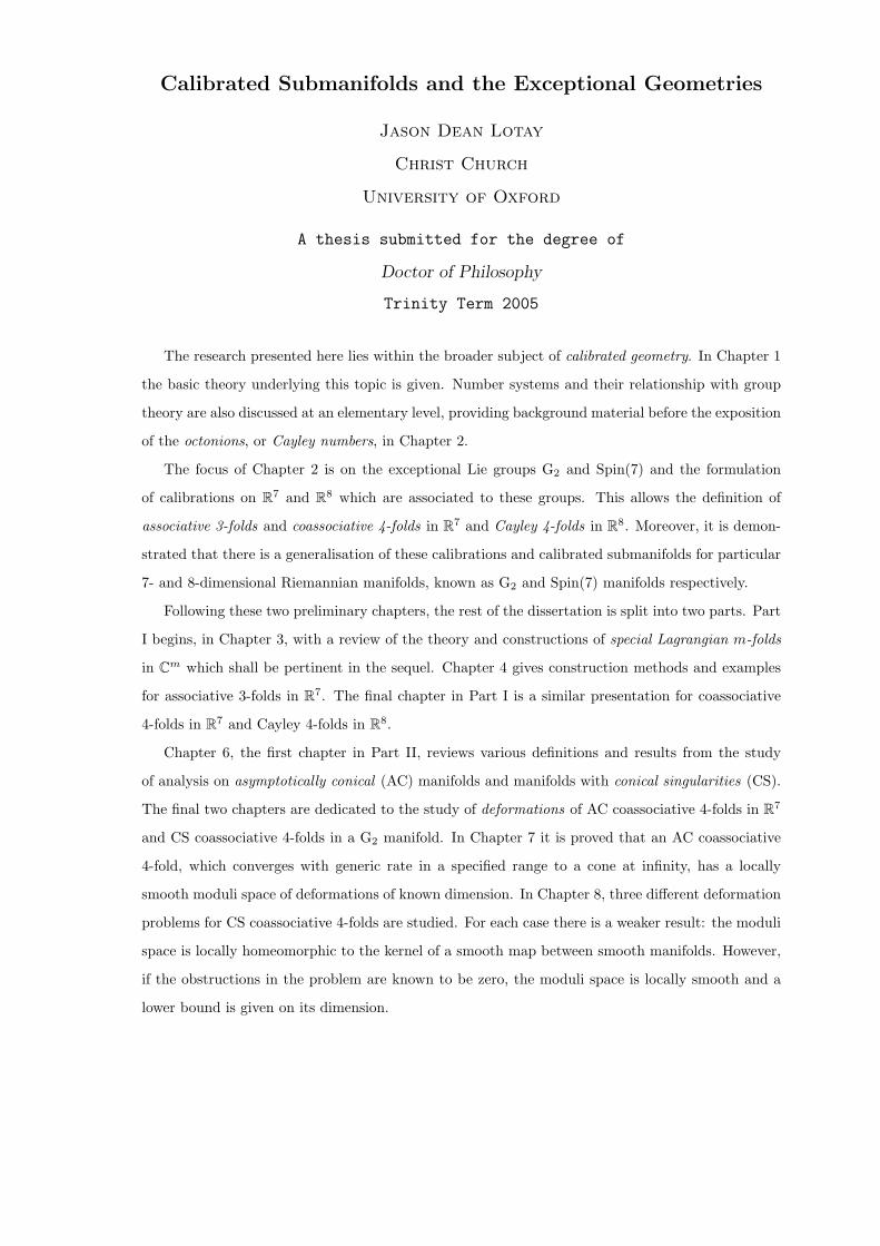
Calibrated Submanifolds and the Exceptional Geometries
Jason Dean Lotay
Christ Church
University of Oxford
A thesis submitted for the degree of
Doctor of Philosophy
Trinity Term 2005
The research presented here lies within the broader subject of calibrated geometry. In Chapter 1
the basic theory underlying this topic is given. Number systems and their relationship with group
theory are also discussed at an elementary level, providing background material before the exposition
of the octonions, or Cayley numbers, in Chapter 2.
The focus of Chapter 2 is on the exceptional Lie groups G2 and Spin(7) and the formulation
of calibrations on R7 and R8 which are associated to these groups. This allows the definition of
associative 3-folds and coassociative 4-folds in R7 and Cayley 4-folds in R8. Moreover, it is demon-
strated that there is a generalisation of these calibrations and calibrated submanifolds for particular
7- and 8-dimensional Riemannian manifolds, known as G2 and Spin(7) manifolds respectively.
Following these two preliminary chapters, the rest of the dissertation is split into two parts. Part
I begins, in Chapter 3, with a review of the theory and constructions of special Lagrangian m-folds
in Cm which shall be pertinent in the sequel. Chapter 4 gives construction methods and examples
for associative 3-folds in R7. The final chapter in Part I is a similar presentation for coassociative
4-folds in R7 and Cayley 4-folds in R8.
Chapter 6, the first chapter in Part II, reviews various definitions and results from the study
of analysis on asymptotically conical (AC) manifolds and manifolds with conical singularities (CS).
The final two chapters are dedicated to the study of deformations of AC coassociative 4-folds in R7
and CS coassociative 4-folds in a G2 manifold. In Chapter 7 it is proved that an AC coassociative
4-fold, which converges with generic rate in a specified range to a cone at infinity, has a locally
smooth moduli space of deformations of known dimension. In Chapter 8, three different deformation
problems for CS coassociative 4-folds are studied. For each case there is a weaker result: the moduli
space is locally homeomorphic to the kernel of a smooth map between smooth manifolds. However,
if the obstructions in the problem are known to be zero, the moduli space is locally smooth and a
lower bound is given on its dimension.


![Geometry of Lagrangian submanifolds related to ...ohnita/2014/BeamerICMSC-RCSOhnita.pdf · [Submanifolds in Riemannian manifolds] (Higher dimensional generalization of curves and](https://static.fdocuments.in/doc/165x107/5edc153fad6a402d66669985/geometry-of-lagrangian-submanifolds-related-to-ohnita2014beamericmsc-submanifolds.jpg)


![arXiv:math/0108088v3 [math.DG] 25 Jun 2002the subject of calibrated submanifolds of Riemannian manifolds with special holonomy is really only beginning to be explored. We begin in](https://static.fdocuments.in/doc/165x107/5edc1537ad6a402d66669977/arxivmath0108088v3-mathdg-25-jun-2002-the-subject-of-calibrated-submanifolds.jpg)


