Calibrated Bayes: spanning the divide between frequentist ...pure Bayesian model selection work, but...

Calibrated Bayes: spanning the

divide between frequentist and

Bayesian inferenceBayesian inference

Roderick J. Little

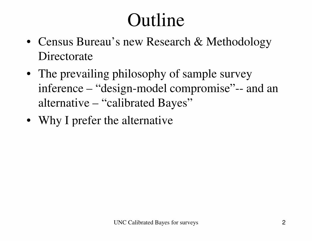
Outline• Census Bureau’s new Research & Methodology

Directorate

• The prevailing philosophy of sample survey

inference – “design-model compromise”-- and an

alternative – “calibrated Bayes”

• Why I prefer the alternative• Why I prefer the alternative

UNC Calibrated Bayes for surveys 2


Directorate






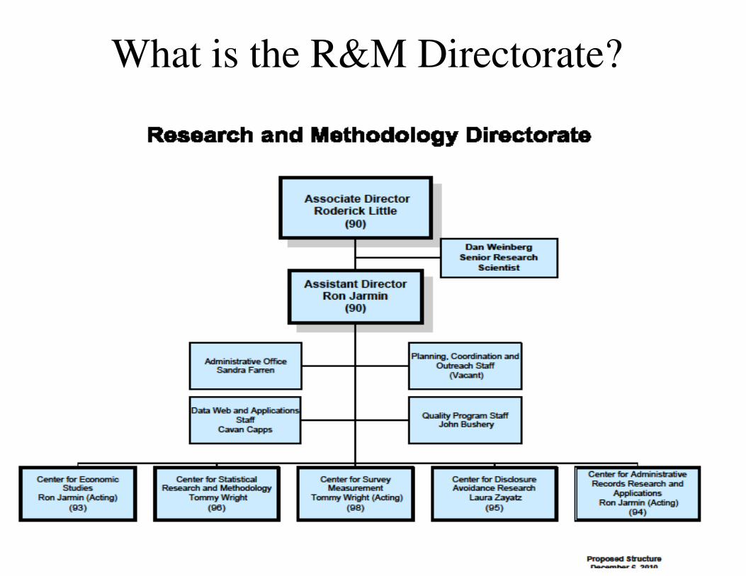
What is the R&M Directorate?


Strategic objectives• Building a Research & Methodology Directorate that

fosters innovation and plays a strategic role in Bureau activities

• Increasing collaborations across Census Bureau directorates - "breaking down the silos"

• Porting research on new products / processes to program areas

• Establishing more robust collaborations with external

5

• Establishing more robust collaborations with external researchers and agencies

• Finding ways to leverage competitive advantages of the Bureau (Title 13, access to admin data) to produce products that have high demand

• Increasing the statistical literacy of Census Bureau data users

UNC Calibrated Bayes for surveys

Some Challenges• Recruit the best researchers

• Build better links between research and production

• Institutionalizing research excellence

• Let people know that the Census Bureau has a new

research directorate with exciting plans!research directorate with exciting plans!

UNC Calibrated Bayes for

surveys

6


Directorate






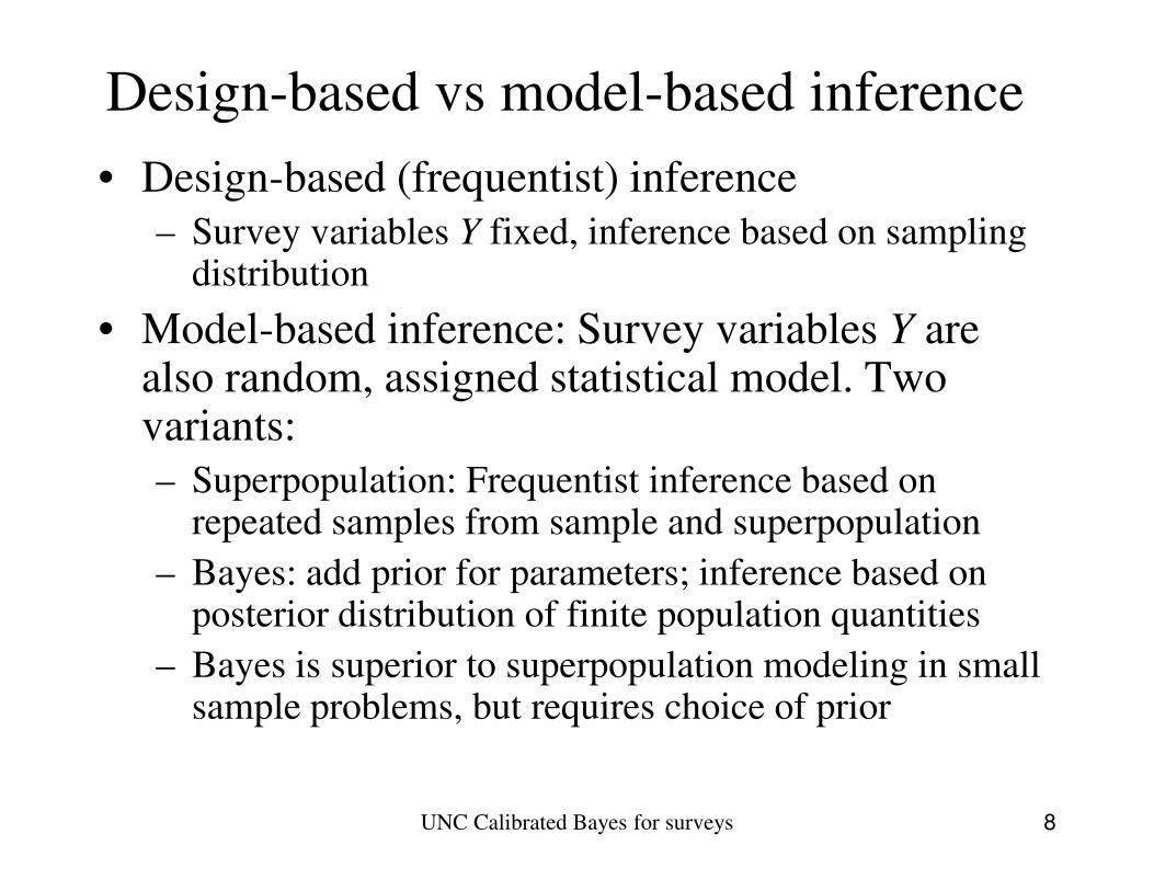
Design-based vs model-based inference

• Design-based (frequentist) inference

– Survey variables Y fixed, inference based on sampling distribution

• Model-based inference: Survey variables Y are also random, assigned statistical model. Two variants:variants:

– Superpopulation: Frequentist inference based on repeated samples from sample and superpopulation

– Bayes: add prior for parameters; inference based on posterior distribution of finite population quantities

– Bayes is superior to superpopulation modeling in small sample problems, but requires choice of prior


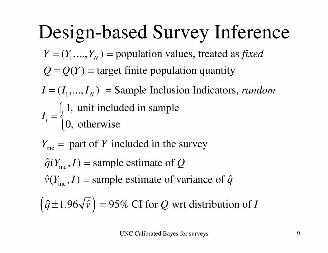
Design-based Survey Inference1( ,..., ) = population values, treated as

( ) = target finite population quantity

NY Y Y fixed

Q Q Y

=

=

1( ,..., ) = Sample Inclusion Indicators,

1, unit included in sample

0, otherwise

N

i

I I I random

I

=

=

( )ˆ ˆ1.96 = 95% CI for wrt distribution of q v Q I±


0, otherwise

inc part of included in the surveyY Y=

inc

inc

ˆ( , ) = sample estimate of

ˆ ˆ( , ) = sample estimate of variance of

q Y I Q

v Y I q

9

Example 1: stratified sampling

1( ) , population mean

/ pop proportion, = pop mean in stratum

J

j jj

j j j

Q Y Y PY

P N N Y Z j

== =

= = =

∑

1

1

Pr( 1) , if , and 0 otherwisejN

j

ji ji j

j i

NI I n

n

−

=

= = =

∑

ˆ( , ) , = sample mean of in stratum J

q Y I y P y y Y j= =∑2 2

st inc 1

2

ˆ ( , ) (1 / ) /

sample variance of in stratum

J

j j j j jj

j

v Y I P n N s n

s Y j

== −

=

∑

( )stˆ1.96 = 95% CI for

sty v Y±

Finite

population

correction


inc st 1ˆ( , ) , = sample mean of in stratum

J

j j jjq Y I y P y y Y j

== =∑

10

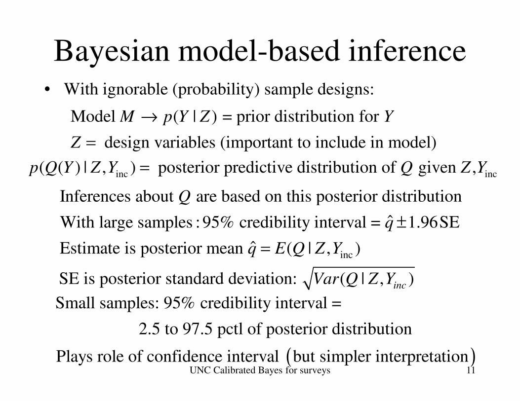
Bayesian model-based inference• With ignorable (probability) sample designs:

Model ( | ) = prior distribution for

design variables (important to include in model)

M p Y Z Y

Z

→

=

inc inc( ( ) | , ) posterior predictive distribution of given ,p Q Y Z Y Q Z Y=

Inferences about are based on this posterior distributionQ


inc

Inferences about are based on this posterior distribution

ˆWith large samples : 95% credibility interval = 1.96SE

ˆEstimate is posterior mean ( | , )

SE is posterior standard deviation: ( | ,

Q

q

q E Q Z Y

Var Q Z Y

±

=

)inc

( )

Small samples: 95% credibility interval =

2.5 to 97.5 pctl of posterior distribution

Plays role of confidence interval but simpler interpretation11

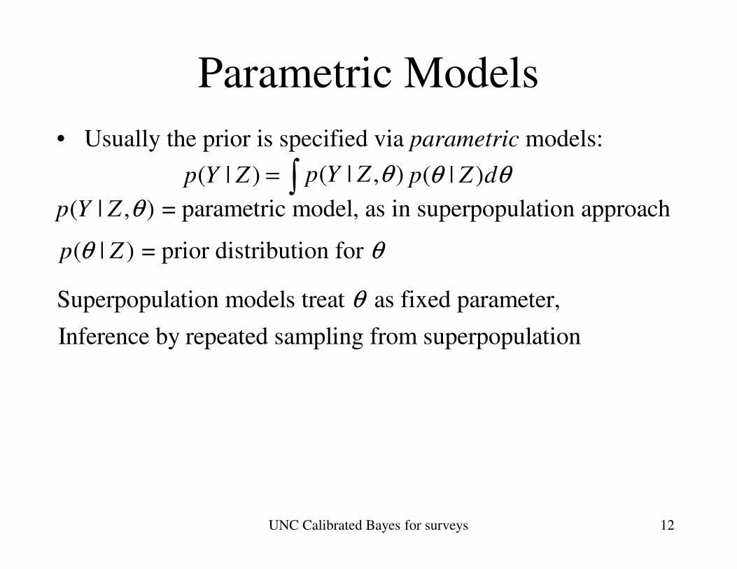
Parametric Models

• Usually the prior is specified via parametric models:

( | ) ( | )p Y Z p Z dθ θ= ∫( | , ) = parametric model, as in superpopulation approachp Y Z θ

( | ) = prior distribution for p Zθ θ

( | , )p Y Z θ


Superpopulation models treat as fixed parameter,

Inference by repeated sampling from superpopulation

θ

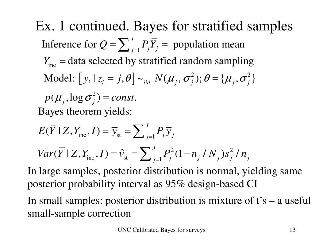
Ex. 1 continued. Bayes for stratified samples

Bayes theorem yields:

( | , , )J

E Y Z Y I y P y= =∑

1Inference for population mean

J

j jjQ PY

== =∑

inc data selected by stratified random samplingY =

[ ] 2 2

2

Model: | , ~ ( , ); { , }

( , log ) .

i i iid j j j j

j j

y z j N

p const

θ µ σ θ µ σ

µ σ

= =

=

In large samples, posterior distribution is normal, yielding same

posterior probability interval as 95% design-based CI

inc st 1

2 2

inc st 1

( | , , )

ˆ( | , , ) (1 / ) /

J

j jj

J

j j j j jj

E Y Z Y I y P y

Var Y Z Y I v P n N s n

=

=

= =

= = −

∑

∑

In small samples: posterior distribution is mixture of t’s – a useful

small-sample correction


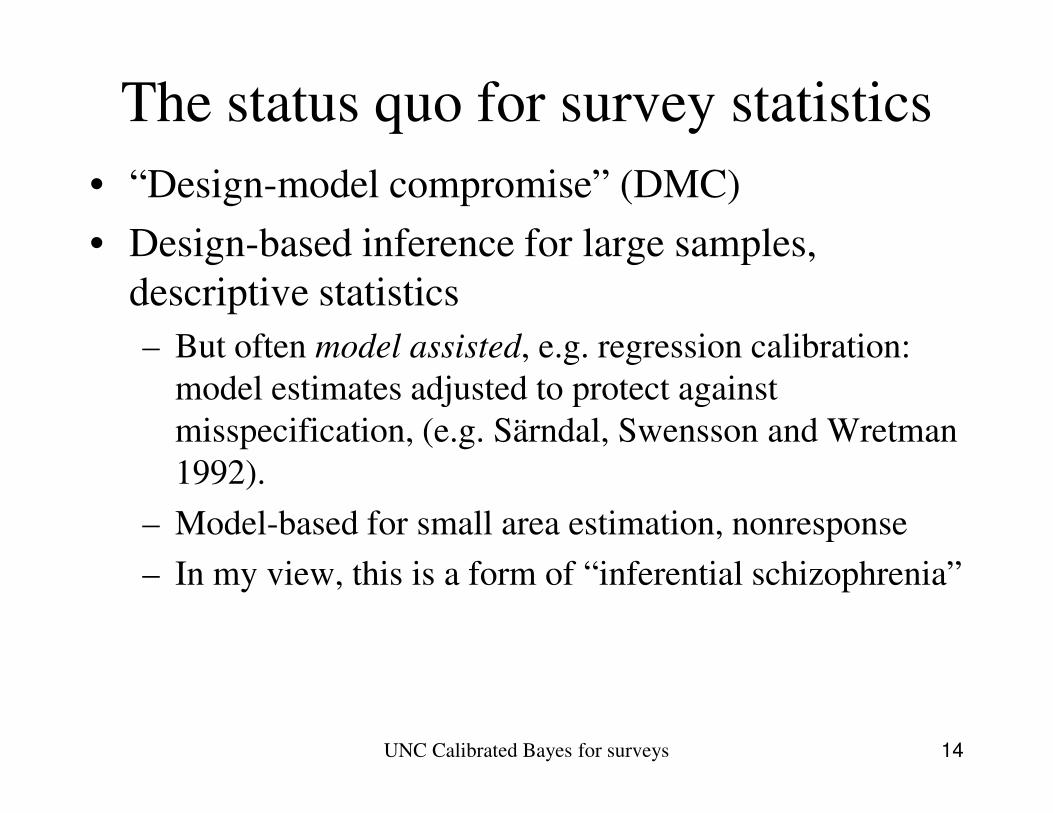
The status quo for survey statistics

• “Design-model compromise” (DMC)

• Design-based inference for large samples,

descriptive statistics

– But often model assisted, e.g. regression calibration:

model estimates adjusted to protect against model estimates adjusted to protect against

misspecification, (e.g. Särndal, Swensson and Wretman

1992).

– Model-based for small area estimation, nonresponse

– In my view, this is a form of “inferential schizophrenia”


Some manifestations of

“inferential schizophrenia” in

the current survey philosophy…


1. Statistical standards

• Census Statistical standards are built from a

design-based perspective

• Economists and other substantive researchers

build models

• I suspect a reason why people bridle at the • I suspect a reason why people bridle at the

standards is that they have a different statistical

philosophy!

• [Economists generally don’t think of themselves

as Bayesian, but to my mind they act like

Bayesians in important respects]


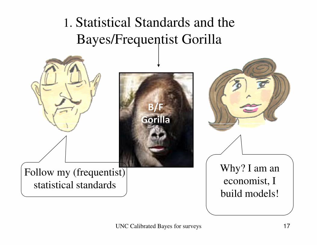
1. Statistical Standards and the

Bayes/Frequentist Gorilla

B/F

GorillaGorilla

Follow my (frequentist)

statistical standards

Why? I am an

economist, I

build models!


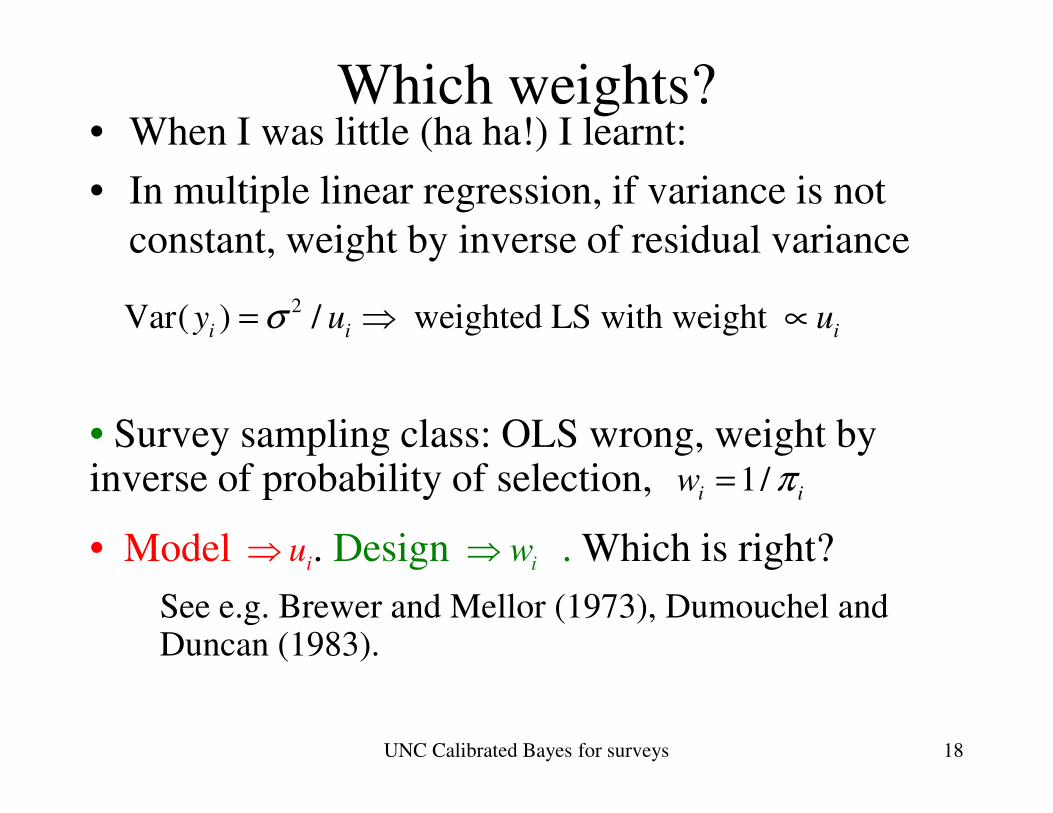
Which weights?• When I was little (ha ha!) I learnt:

• In multiple linear regression, if variance is not

constant, weight by inverse of residual variance

2Var( ) / weighted LS with weight i i i

y u uσ= ⇒ ∝

See e.g. Brewer and Mellor (1973), Dumouchel and Duncan (1983).

• Model . Design . Which is right?

• Survey sampling class: OLS wrong, weight by inverse of probability of selection, 1/

i iw π=

iu⇒

iw⇒


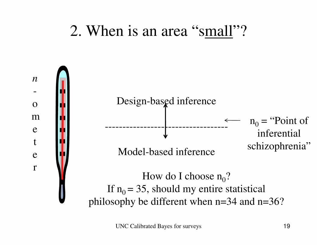
2. When is an area “small”?

n

-

o

m

Design-based inference

-----------------------------------n0 = “Point of


e

t

e

r

-----------------------------------

Model-based inference

n0 = “Point of

inferential

schizophrenia”

How do I choose n0?

If n0 = 35, should my entire statistical

philosophy be different when n=34 and n=36?

19

• Towards the alternative: Calibrated Bayes.• Towards the alternative: Calibrated Bayes.


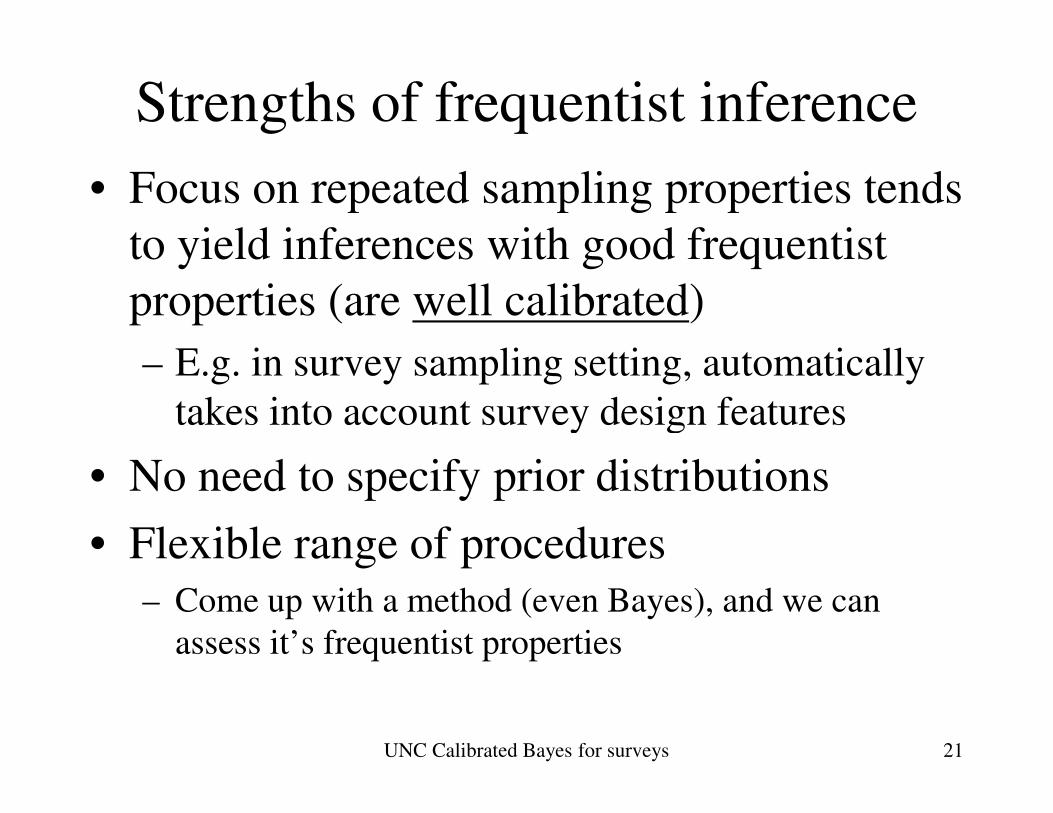
Strengths of frequentist inference

• Focus on repeated sampling properties tends

to yield inferences with good frequentist

properties (are well calibrated)

– E.g. in survey sampling setting, automatically

takes into account survey design featurestakes into account survey design features

• No need to specify prior distributions

• Flexible range of procedures

– Come up with a method (even Bayes), and we can

assess it’s frequentist properties


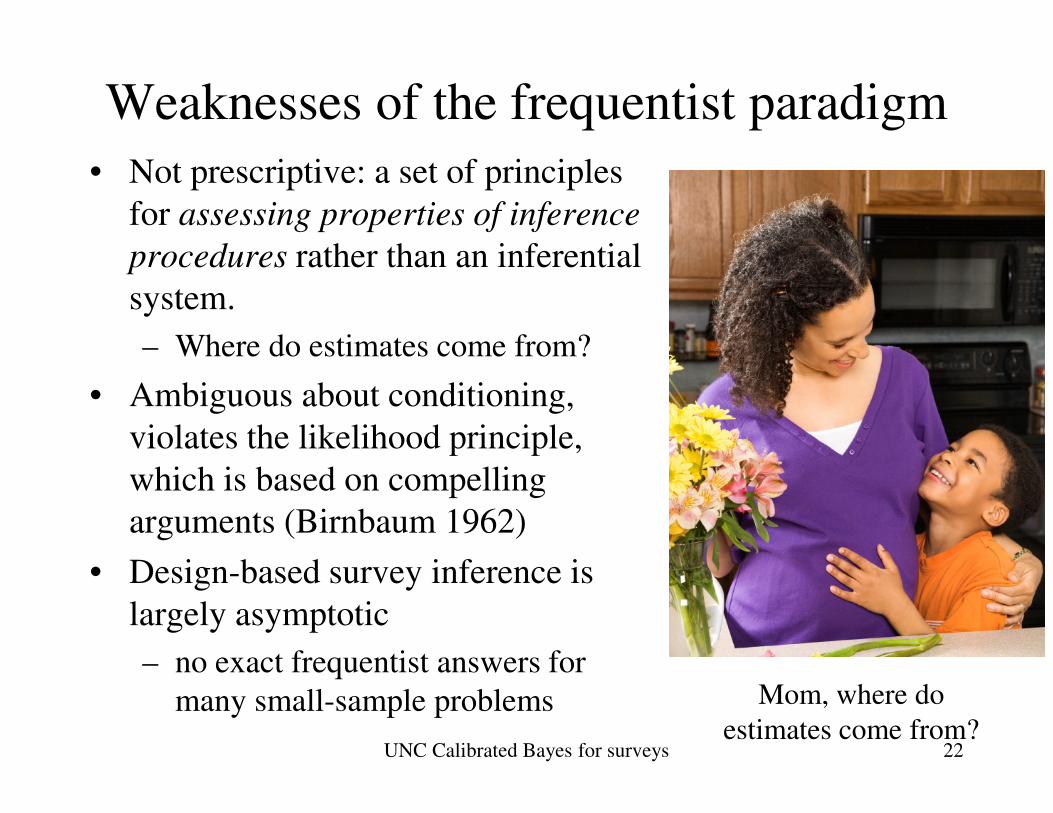
Weaknesses of the frequentist paradigm

• Not prescriptive: a set of principles

for assessing properties of inference

procedures rather than an inferential

system.

– Where do estimates come from?

• Ambiguous about conditioning, • Ambiguous about conditioning,

violates the likelihood principle,

which is based on compelling

arguments (Birnbaum 1962)

• Design-based survey inference is

largely asymptotic

– no exact frequentist answers for

many small-sample problems


Mom, where do

estimates come from?

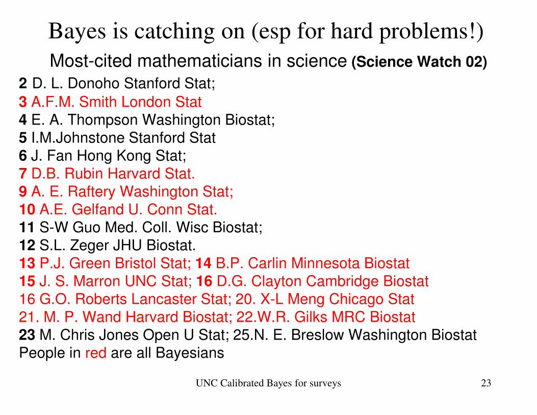
Bayes is catching on (esp for hard problems!)

Most-cited mathematicians in science (Science Watch 02)

2 D. L. Donoho Stanford Stat;

3 A.F.M. Smith London Stat

4 E. A. Thompson Washington Biostat;

5 I.M.Johnstone Stanford Stat

6 J. Fan Hong Kong Stat;

7 D.B. Rubin Harvard Stat.

9 A. E. Raftery Washington Stat;

10 A.E. Gelfand U. Conn Stat. 10 A.E. Gelfand U. Conn Stat.

11 S-W Guo Med. Coll. Wisc Biostat;

12 S.L. Zeger JHU Biostat.

13 P.J. Green Bristol Stat; 14 B.P. Carlin Minnesota Biostat

15 J. S. Marron UNC Stat; 16 D.G. Clayton Cambridge Biostat

16 G.O. Roberts Lancaster Stat; 20. X-L Meng Chicago Stat

21. M. P. Wand Harvard Biostat; 22.W.R. Gilks MRC Biostat

23 M. Chris Jones Open U Stat; 25.N. E. Breslow Washington Biostat

People in red are all Bayesians


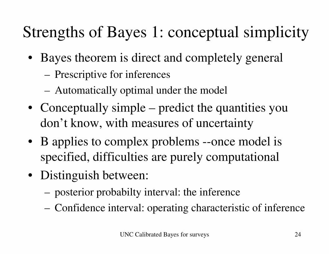
Strengths of Bayes 1: conceptual simplicity

• Bayes theorem is direct and completely general

– Prescriptive for inferences

– Automatically optimal under the model

• Conceptually simple – predict the quantities you

don’t know, with measures of uncertaintydon’t know, with measures of uncertainty

• B applies to complex problems --once model is

specified, difficulties are purely computational

• Distinguish between:

– posterior probabilty interval: the inference

– Confidence interval: operating characteristic of inference


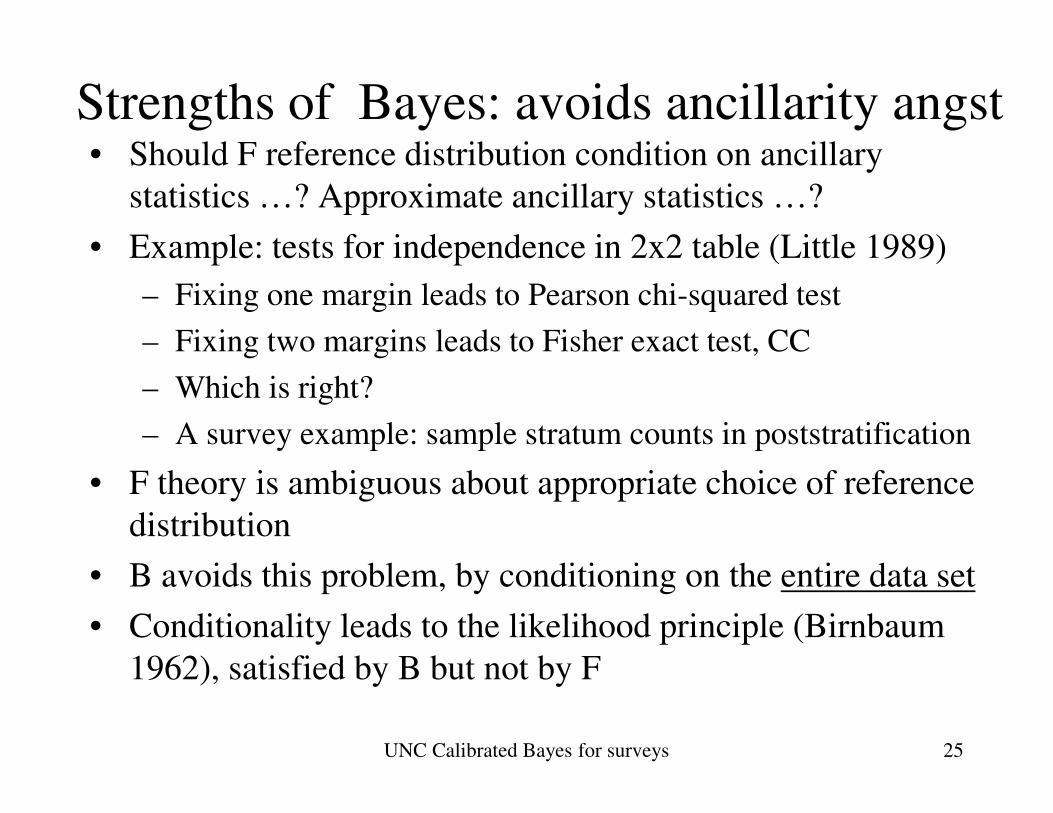
Strengths of Bayes: avoids ancillarity angst• Should F reference distribution condition on ancillary

statistics …? Approximate ancillary statistics …?

• Example: tests for independence in 2x2 table (Little 1989)

– Fixing one margin leads to Pearson chi-squared test

– Fixing two margins leads to Fisher exact test, CC

– Which is right?

– A survey example: sample stratum counts in poststratification

• F theory is ambiguous about appropriate choice of reference

distribution

• B avoids this problem, by conditioning on the entire data set

• Conditionality leads to the likelihood principle (Birnbaum

1962), satisfied by B but not by F


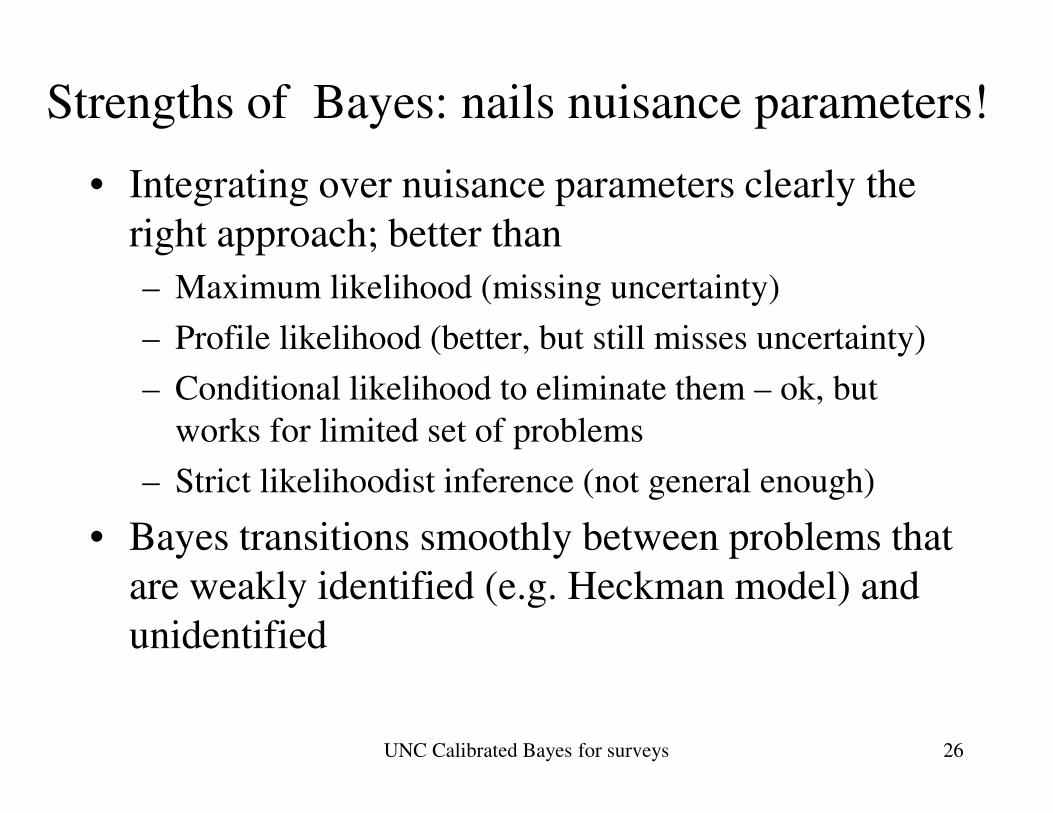
Strengths of Bayes: nails nuisance parameters!

• Integrating over nuisance parameters clearly the

right approach; better than

– Maximum likelihood (missing uncertainty)

– Profile likelihood (better, but still misses uncertainty)

– Conditional likelihood to eliminate them – ok, but – Conditional likelihood to eliminate them – ok, but

works for limited set of problems

– Strict likelihoodist inference (not general enough)

• Bayes transitions smoothly between problems that

are weakly identified (e.g. Heckman model) and

unidentified


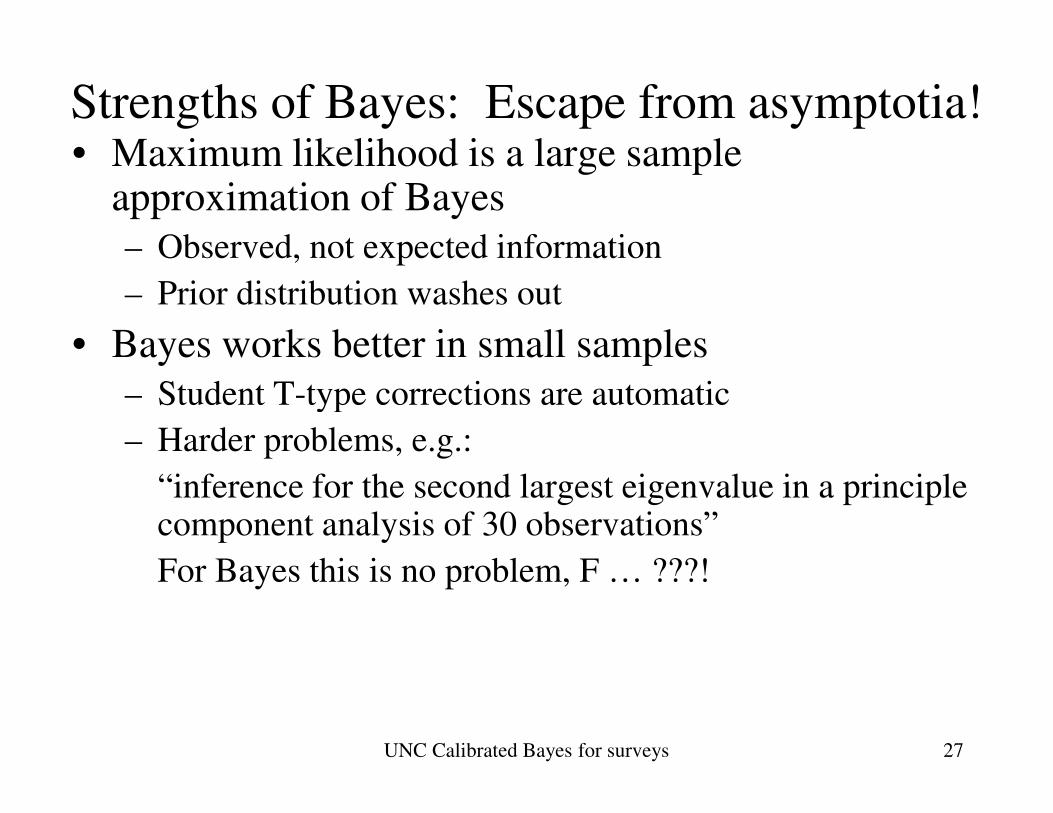
Strengths of Bayes: Escape from asymptotia!• Maximum likelihood is a large sample

approximation of Bayes

– Observed, not expected information

– Prior distribution washes out

• Bayes works better in small samples

– Student T-type corrections are automatic– Student T-type corrections are automatic

– Harder problems, e.g.:

“inference for the second largest eigenvalue in a principle component analysis of 30 observations”

For Bayes this is no problem, F … ???!


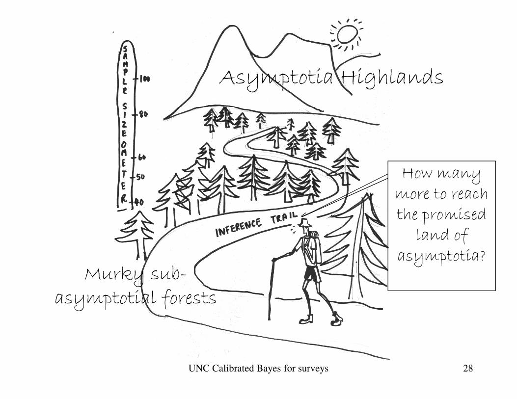
Asymptotia Highlands

How many more to reach

Murky sub-asymptotial forests

more to reach the promised land of

asymptotia?


The “standard error” error• Design-based survey methods assume large samples,

often report estimates and standard errors (or margins of error, coefficients of variation)

• This implicitly assumes “estimate +/- z* se” is a valid confidence interval (e.g. z = 1.96 for 95% interval)

• But in small samples, this is not true, so

• The goal is confidence intervals that have the • The goal is confidence intervals that have the approximate nominal coverage, not estimates and standard errors• As a calibrated Bayesian I would say probability intervals

with the correct confidence coverage, but since regular people interpret confidence intervals like probability intervals the distinction is practically moot.


Weakness of B: where do models come from?

• B is less effective for model formulation and assessment than for inference under a model.

• For example, Bayesian hypothesis testing for comparing models of different dimension is tricky

– sensitive to choice of priors; can’t just slap down a reference priorreference prior

– “Hard-line” subjective Bayesians claim they can make pure Bayesian model selection work, but this approach is a hard sell for scientific inference

– Most use the data for model selection, in some form

– Model formulation and assessment will never achieve the degree of clarity of Bayesian inference under an agreed model


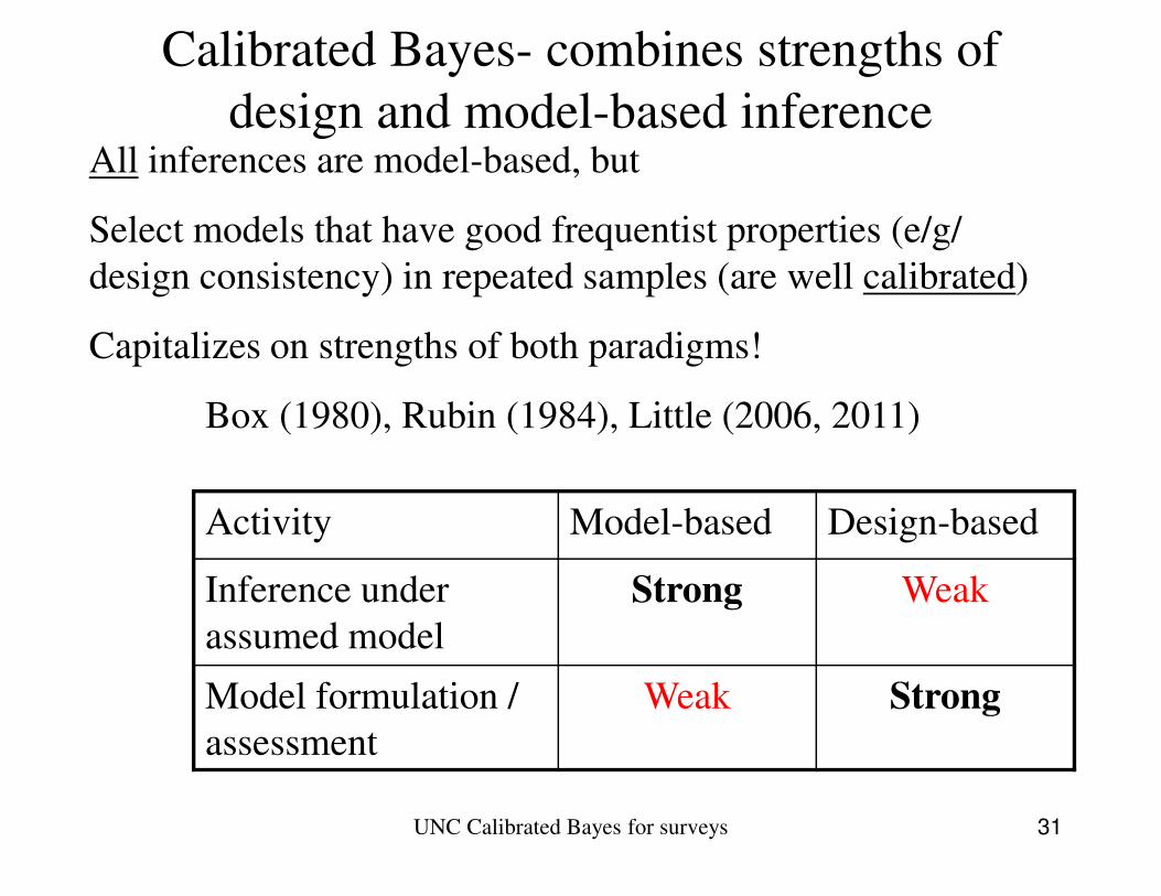
Calibrated Bayes- combines strengths of

design and model-based inferenceAll inferences are model-based, but

Select models that have good frequentist properties (e/g/

design consistency) in repeated samples (are well calibrated)

Capitalizes on strengths of both paradigms!

Box (1980), Rubin (1984), Little (2006, 2011)

Activity Model-based Design-based

Inference under

assumed model

Strong Weak

Model formulation /

assessment

Weak Strong


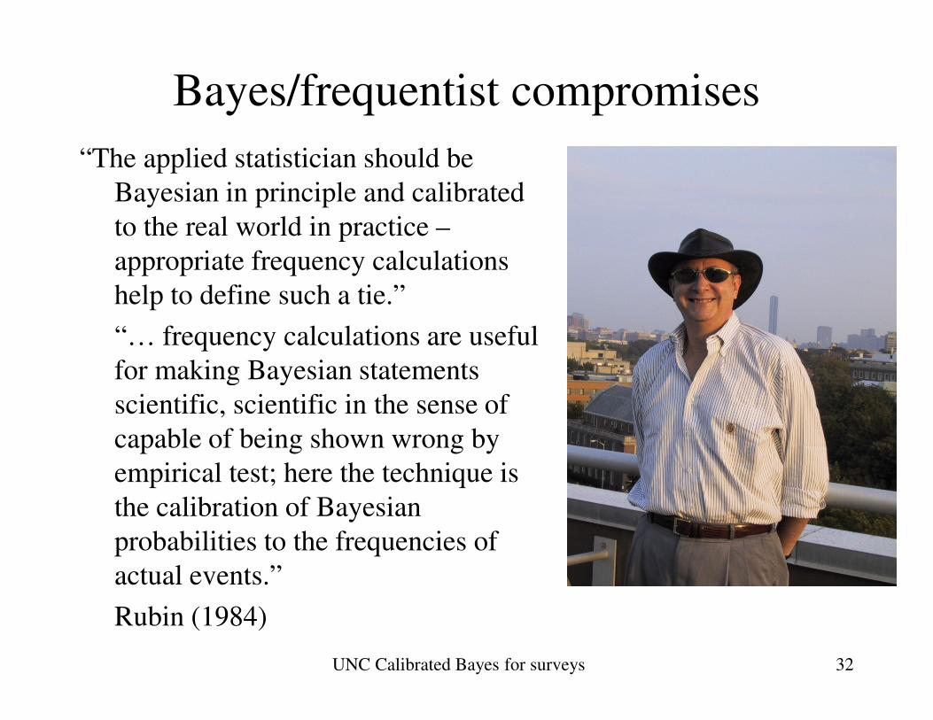
Bayes/frequentist compromises

“The applied statistician should be

Bayesian in principle and calibrated

to the real world in practice –

appropriate frequency calculations

help to define such a tie.”

“… frequency calculations are useful

for making Bayesian statements


for making Bayesian statements

scientific, scientific in the sense of

capable of being shown wrong by

empirical test; here the technique is

the calibration of Bayesian

probabilities to the frequencies of

actual events.”

Rubin (1984)

Applications of Calibrated Bayes

• Small Area Estimation: SAIPE

• Inference for Proportion from PPS samples

• Survey Weights derived from a Bayes Model


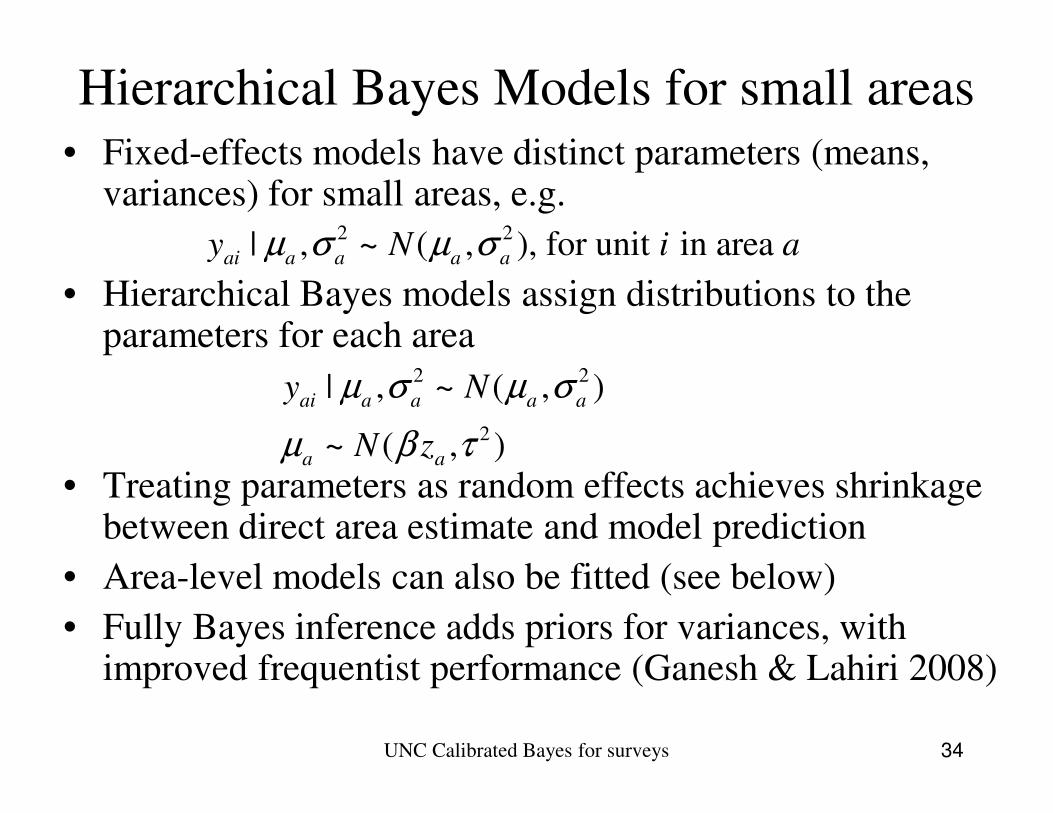
Hierarchical Bayes Models for small areas

• Fixed-effects models have distinct parameters (means, variances) for small areas, e.g.

• Hierarchical Bayes models assign distributions to the parameters for each area

2 2| , ~ ( , )ai a a a ay Nµ σ µ σ

2 2| , ~ ( , ), for unit in area ai a a a ay N i aµ σ µ σ

• Treating parameters as random effects achieves shrinkage between direct area estimate and model prediction

• Area-level models can also be fitted (see below)

• Fully Bayes inference adds priors for variances, with improved frequentist performance (Ganesh & Lahiri 2008)


2~ ( , )

ai a a a a

a aN zµ β τ

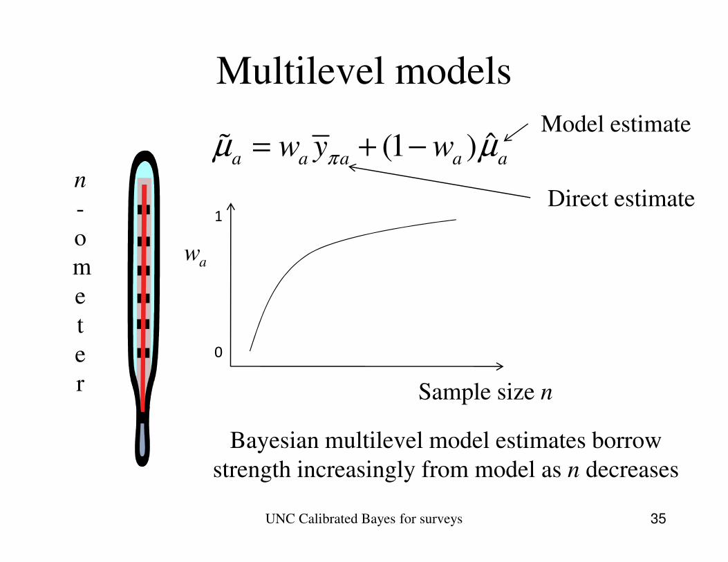
Multilevel models

n

-

o

m

ˆ(1 )a a a a aw y wπµ µ= + −ɶ

aw

1

Model estimate

Direct estimate


e

t

e

r

Bayesian multilevel model estimates borrow

strength increasingly from model as n decreases

35

0

Sample size n

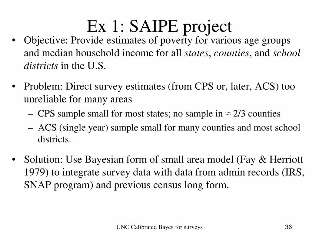
Ex 1: SAIPE project• Objective: Provide estimates of poverty for various age groups

and median household income for all states, counties, and school

districts in the U.S.

• Problem: Direct survey estimates (from CPS or, later, ACS) too

unreliable for many areas

– CPS sample small for most states; no sample in ≈ 2/3 counties

– ACS (single year) sample small for many counties and most school – ACS (single year) sample small for many counties and most school

districts.

• Solution: Use Bayesian form of small area model (Fay & Herriott

1979) to integrate survey data with data from admin records (IRS,

SNAP program) and previous census long form.


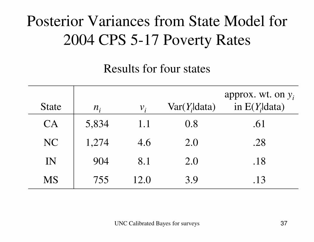
Posterior Variances from State Model for

2004 CPS 5-17 Poverty Rates

Results for four states

State ni vi Var(Yi|data)

approx. wt. on yi

in E(Yi|data)

CA 5,834 1.1 0.8 .61


CA 5,834 1.1 0.8 .61

NC 1,274 4.6 2.0 .28

IN 904 8.1 2.0 .18

MS 755 12.0 3.9 .13

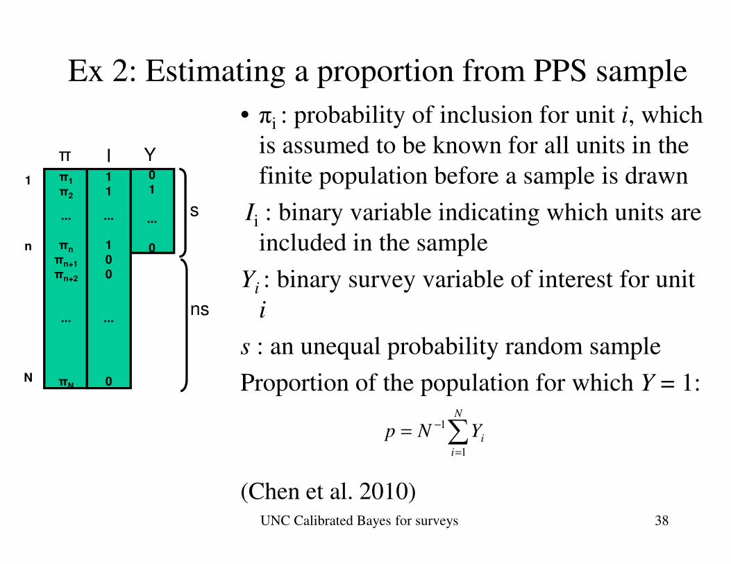
Ex 2: Estimating a proportion from PPS sample

• πi : probability of inclusion for unit i, which

is assumed to be known for all units in the

finite population before a sample is drawn

Ii : binary variable indicating which units are

included in the sample

Yi : binary survey variable of interest for unit

π1

π2

...

πn

πn+1

πn+2

0

1

...

0

1

n

π Y

s

1

1

...

1

0

0

I

∑=

−=N

i

iYNp1

1

Yi : binary survey variable of interest for unit

i

s : an unequal probability random sample

Proportion of the population for which Y = 1:

(Chen et al. 2010)

n+2

...

πNN

ns...

0


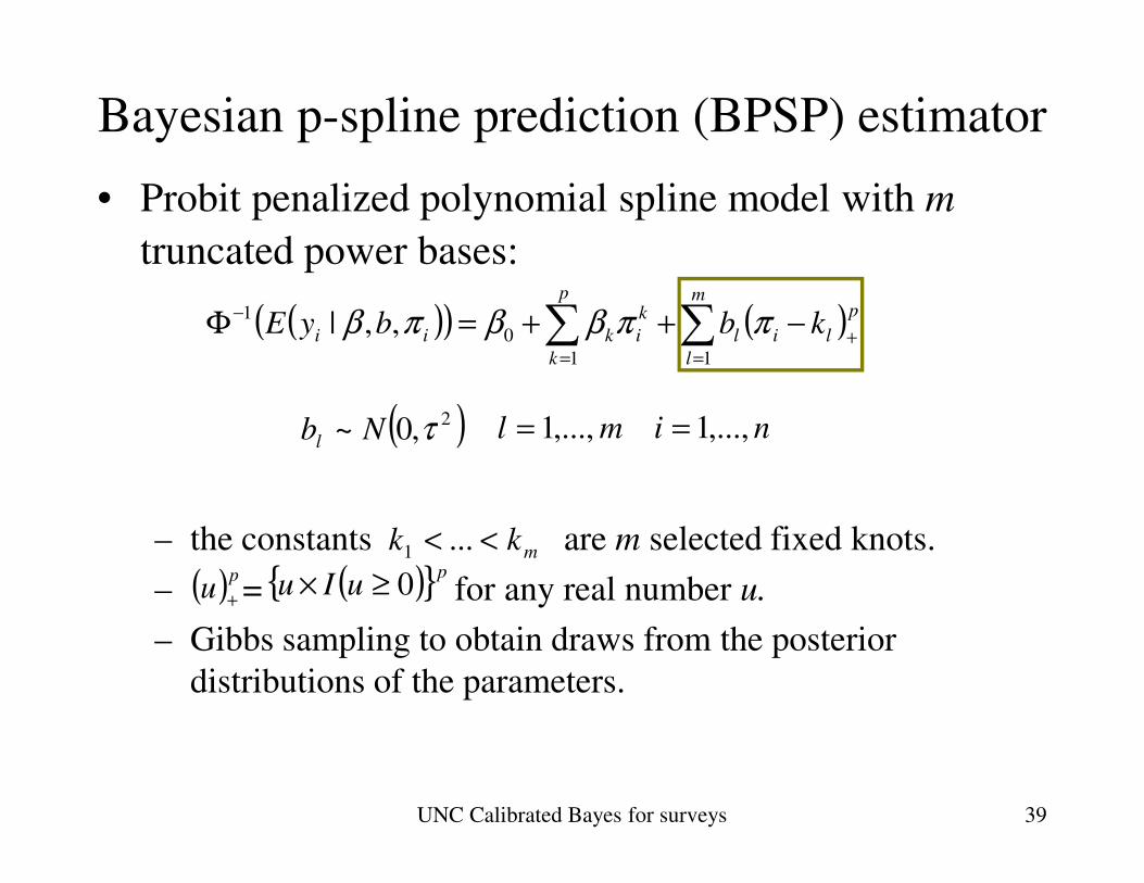
Bayesian p-spline prediction (BPSP) estimator

• Probit penalized polynomial spline model with m

truncated power bases:

( )( ) ( )p

li

m

l

l

p

k

k

ikii kbbyE+

==

− −++=Φ ∑∑ ππββπβ11

0

1 ,,|

( )2,0~ τNblml ,...,1= ni ,...,1=

– the constants are m selected fixed knots.

– = for any real number u.

– Gibbs sampling to obtain draws from the posterior

distributions of the parameters.

( ),0~ τNblml ,...,1= ni ,...,1=

mkk << ...1

( )pu +

( ){ }puIu 0≥×


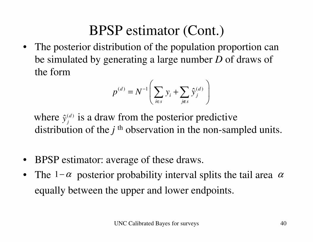
BPSP estimator (Cont.)• The posterior distribution of the population proportion can

be simulated by generating a large number D of draws of

the form

where is a draw from the posterior predictive

( ) 1 ( )ˆd d

i j

i s j s

p N y y−

∈ ∉

= +

∑ ∑

( )ˆ d

jywhere is a draw from the posterior predictive

distribution of the j th observation in the non-sampled units.

• BPSP estimator: average of these draws.

• The posterior probability interval splits the tail area

equally between the upper and lower endpoints.

ˆjy

α−1 α


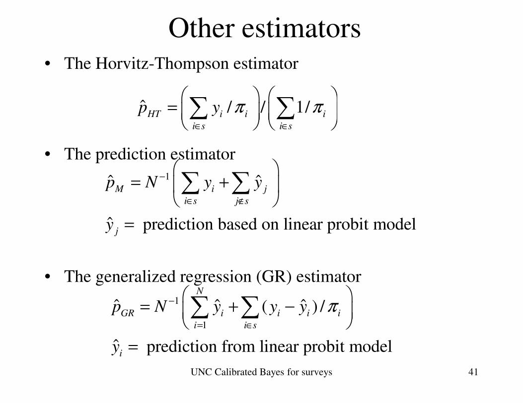
Other estimators • The Horvitz-Thompson estimator

• The prediction estimator

ˆ / / 1/HT i i i

i s i s

p y π π∈ ∈

= ∑ ∑

1ˆ ˆM i j

i s j s

p N y y−

∈ ∉

= +

∑ ∑

• The generalized regression (GR) estimator

1

1

ˆ ˆ ˆ( ) /

ˆ prediction from linear probit model

N

GR i i i i

i i s

i

p N y y y

y

π−

= ∈

= + −

=

∑ ∑

ˆ prediction based on linear probit model

i s j s

jy

∈ ∉

=


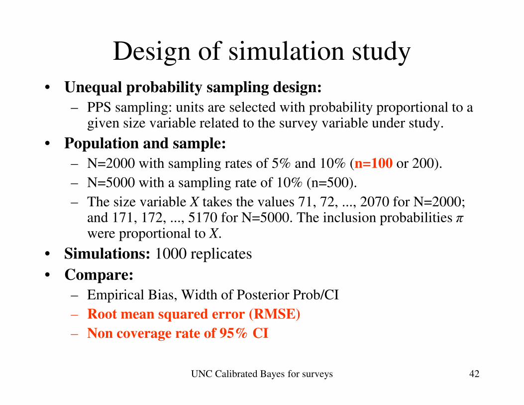
Design of simulation study

• Unequal probability sampling design:

– PPS sampling: units are selected with probability proportional to a given size variable related to the survey variable under study.

• Population and sample:

– N=2000 with sampling rates of 5% and 10% (n=100 or 200).

– N=5000 with a sampling rate of 10% (n=500).

– The size variable X takes the values 71, 72, ..., 2070 for N=2000; – The size variable X takes the values 71, 72, ..., 2070 for N=2000; and 171, 172, ..., 5170 for N=5000. The inclusion probabilities πwere proportional to X.

• Simulations: 1000 replicates

• Compare:

– Empirical Bias, Width of Posterior Prob/CI

– Root mean squared error (RMSE)

– Non coverage rate of 95% CI


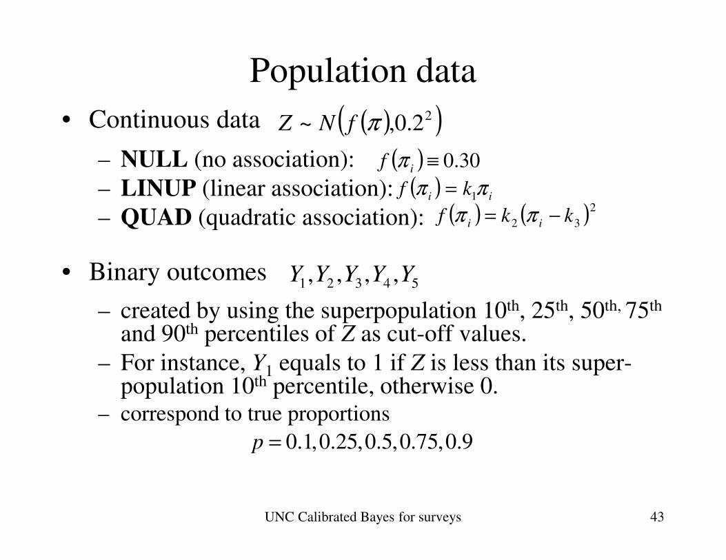
Population data

• Continuous data

– NULL (no association):

– LINUP (linear association):

– QUAD (quadratic association):

• Binary outcomes

( ) 30.0≡if π

( ) ii kf ππ 1=

( ) ( )2

32 kkf ii −= ππ

( )( )22.0,~ πfNZ

1 2 3 4 5, , , ,Y Y Y Y Y• Binary outcomes

– created by using the superpopulation 10th, 25th, 50th, 75th

and 90th percentiles of Z as cut-off values.

– For instance, Y1 equals to 1 if Z is less than its super-population 10th percentile, otherwise 0.

– correspond to true proportions

1 2 3 4 5, , , ,Y Y Y Y Y

0.1,0.25,0.5,0.75,0.9p =


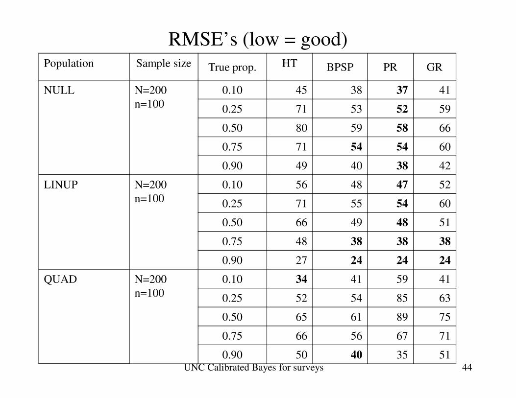
RMSE’s (low = good)Population Sample size True prop. HT BPSP PR GR

NULL N=200

n=100

0.10 45 38 37 41

0.25 71 53 52 59

0.50 80 59 58 66

0.75 71 54 54 60

0.90 49 40 38 42

LINUP N=200

n=100

0.10 56 48 47 52

0.25 71 55 54 60n=100 0.25 71 55 54 60

0.50 66 49 48 51

0.75 48 38 38 38

0.90 27 24 24 24

QUAD N=200

n=100

0.10 34 41 59 41

0.25 52 54 85 63

0.50 65 61 89 75

0.75 66 56 67 71

0.90 50 40 35 51UNC Calibrated Bayes for surveys 44

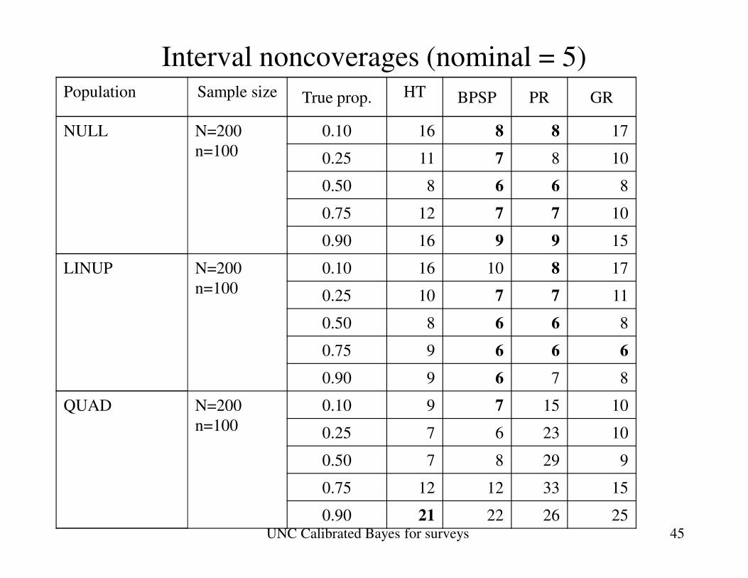
Interval noncoverages (nominal = 5)Population Sample size True prop. HT BPSP PR GR

NULL N=200

n=100

0.10 16 8 8 17

0.25 11 7 8 10

0.50 8 6 6 8

0.75 12 7 7 10

0.90 16 9 9 15

LINUP N=200

n=100

0.10 16 10 8 17

0.25 10 7 7 11n=100 0.25 10 7 7 11

0.50 8 6 6 8

0.75 9 6 6 6

0.90 9 6 7 8

QUAD N=200

n=100

0.10 9 7 15 10

0.25 7 6 23 10

0.50 7 8 29 9

0.75 12 12 33 15

0.90 21 22 26 25UNC Calibrated Bayes for surveys 45

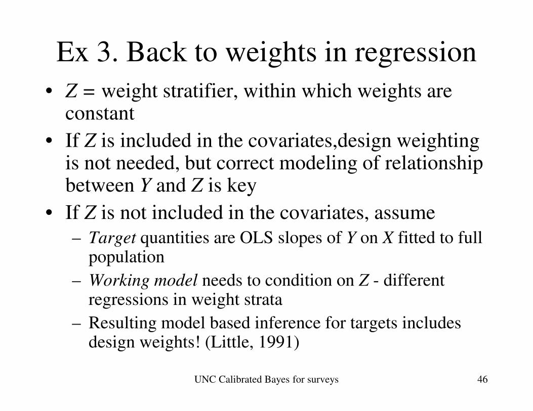
Ex 3. Back to weights in regression

• Z = weight stratifier, within which weights are constant

• If Z is included in the covariates,design weighting is not needed, but correct modeling of relationship between Y and Z is key

• If Z is not included in the covariates, assume


• If Z is not included in the covariates, assume

– Target quantities are OLS slopes of Y on X fitted to full population

– Working model needs to condition on Z - different regressions in weight strata

– Resulting model based inference for targets includes design weights! (Little, 1991)

Summary

• Philosophies of inference matter!

– A cohesive philosophy of statistics would be nice!

• Bayes and frequentist ideas are both important for

good statistical inference

• The calibrated Bayes compromise capitalizes on • The calibrated Bayes compromise capitalizes on

strengths of Bayes and frequentist paradigms

• Focused on survey inference, but these ideas are

for me a roadmap for statistics in general


ReferencesBirnbaum, A. (1962), “On the Foundations of Statistical Inference” , JASA, 57, 269–326.

Box, GEP (1980), “Sampling and Bayes inference in scientific modelling and robustness” (with discussion), JRSSA 143, 383-430.

Brewer, KRW. & Mellor, RW (1973), "The effect of sample structure on analytical surveys," Australian J. Statist. 15, 145-152.

Chen, Q., Elliott, MR. & Little, RJ. (2010). Bayesian Penalized Spline Model-Based Estimation of the Finite Population Proportion for Probability-Proportional-to-Size Samples. Surv. Meth. 36, 23-34.

Dumouchel, WH. and Duncan, GJ. (1983), "Using survey weights in multiple regression analysis of stratified samples," JASA, 78, 535-543.

Ganesh, N. & Lahiri, P. (2008). ”A new class of average moment matching priors,” Biometrika, 95, 2,

514–520

Little, RJ (1989). “On testing the equality of two independent binomial proportions,” Am.Statist., 43, Little, RJ (1989). “On testing the equality of two independent binomial proportions,” Am.Statist., 43, 283-288.

Little, RJ (1991), “Inference with survey weights,” JOS, 7, 405-424.

Little, RJ (2006). “Calibrated Bayes: A Bayes/Frequentist Roadmap.” Am.Statist., 60, 3, 213-223.

Little, RJ (2011). “Calibrated Bayes, for Statistics in General, and Missing Data in Particular” with

discussion and rejoinder. In press, Statist. Sci.

Rubin, DB (1984), “Bayesianly justifiable and relevant frequency calculations for the applied statistician”, Ann. Statist. 12, 1151-1172.

Särndal, C-E, Swensson, B & Wretman, JH. (1992), Model Assisted Survey Sampling, Springer Verlag: New York.


and thanks to my recent students…Hyonggin An, Qi Long, Ying Yuan, Guangyu Zhang, Xiaoxi

Zhang, Di An, Yan Zhou, Rebecca Andridge, Qixuan Chen,

Ying Guo, Chia-Ning Wang, Nanhua Zhang

UNC 2011 SSIL 49

Calibrated Bayes: spanning the divide between frequentist ...pure Bayesian model selection work, but...

Documents

Transcript of Calibrated Bayes: spanning the divide between frequentist ...pure Bayesian model selection work, but...