Calibrate Rotameter and Orifice Meter and Explore Reynoldsfmorriso/cm3215/Lectures/CM...Lab:...
13
Calibrate Flow Meters Lab, CM3215 F. Morrison 1 CM3215 Fundamentals of Chemical Engineering Laboratory Professor Faith Morrison Department of Chemical Engineering Michigan Technological University Calibrate Rotameter and Orifice Meter and Explore Reynolds # © Faith A. Morrison, Michigan Tech U. 1 © Faith A. Morrison, Michigan Tech U. Image source: www.cheresources.com/flowmeas.shtml Orifice Flow Meters • Obstruct flow • Build upstream pressure • Δ is a function of 2
Transcript of Calibrate Rotameter and Orifice Meter and Explore Reynoldsfmorriso/cm3215/Lectures/CM...Lab:...
Calibrate Flow Meters Lab, CM3215 F. Morrison
1
CM3215
Fundamentals of Chemical Engineering Laboratory
Professor Faith Morrison
Department of Chemical EngineeringMichigan Technological University
Calibrate Rotameter and Orifice Meter and Explore
Reynolds #
© Faith A. Morrison, Michigan Tech U.
1
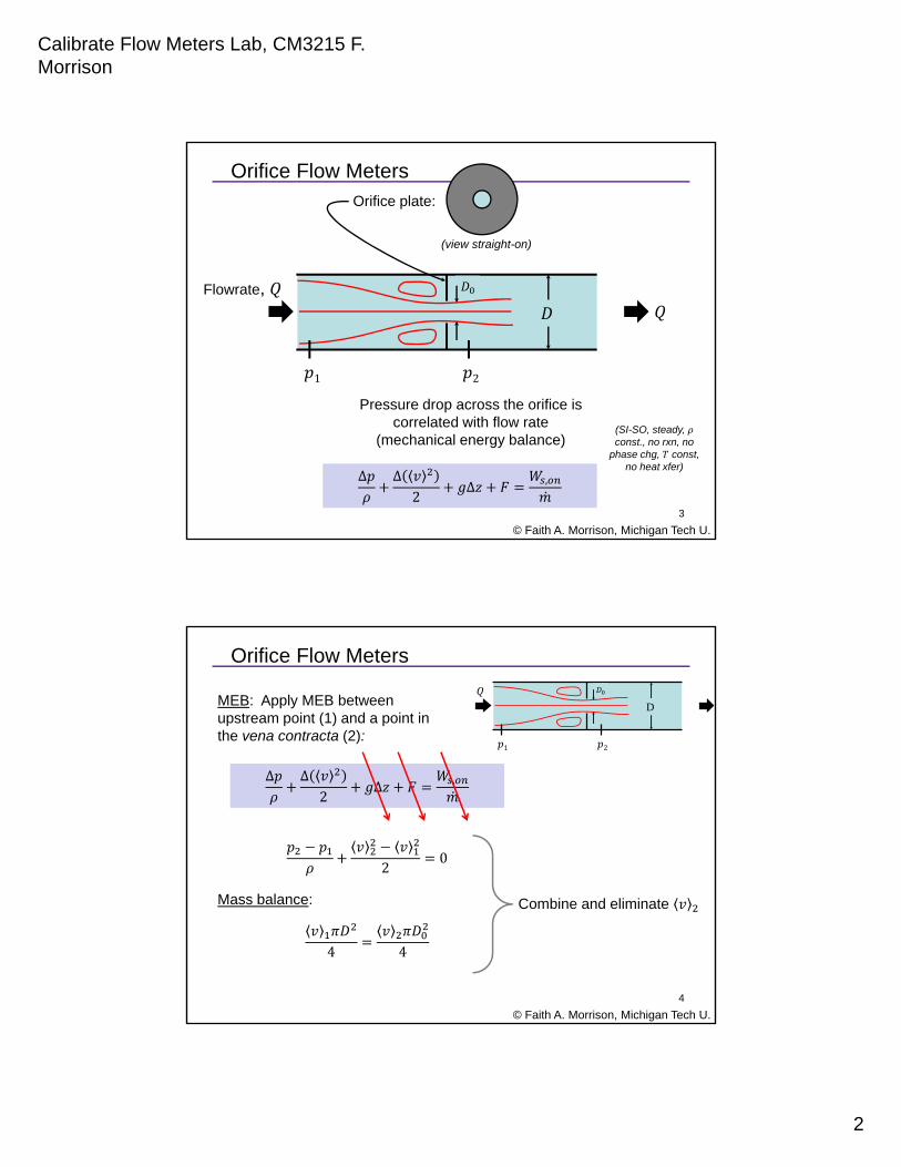
© Faith A. Morrison, Michigan Tech U.Image source: www.cheresources.com/flowmeas.shtml
Orifice Flow Meters
• Obstruct flow• Build upstream pressure• Δ is a function of
2
Calibrate Flow Meters Lab, CM3215 F. Morrison
2
© Faith A. Morrison, Michigan Tech U.
Pressure drop across the orifice is correlated with flow rate
(mechanical energy balance)
Orifice Flow Meters
1 2
Orifice plate:
Flowrate,
Δ Δ2
Δ ,
3
(view straight-on)
(SI-SO, steady, const., no rxn, no
phase chg, const, no heat xfer)
© Faith A. Morrison, Michigan Tech U.
Orifice Flow Meters
Δ Δ2
Δ ,
DMEB: Apply MEB between upstream point (1) and a point in the vena contracta (2):
20
Mass balance:
4 4
Combine and eliminate
4
Calibrate Flow Meters Lab, CM3215 F. Morrison
3
© Faith A. Morrison, Michigan Tech U.
Orifice Flow Meters
D
4
2
1
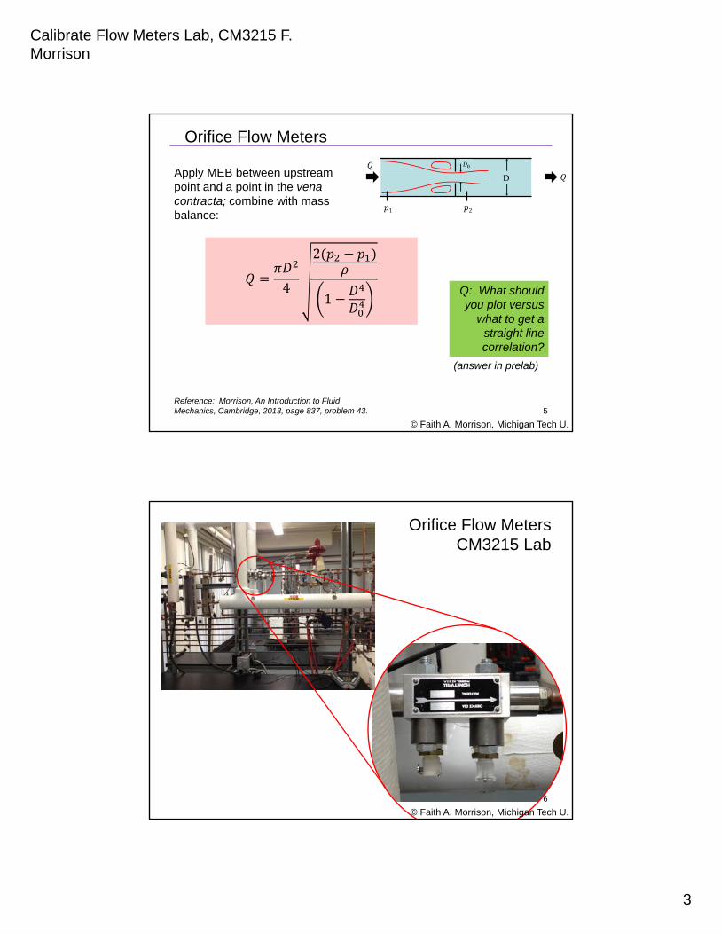
Reference: Morrison, An Introduction to Fluid Mechanics, Cambridge, 2013, page 837, problem 43.
Apply MEB between upstream point and a point in the vena contracta; combine with mass balance:
Q: What should you plot versus
what to get a straight line correlation?
5
(answer in prelab)
Orifice Flow Meters CM3215 Lab
© Faith A. Morrison, Michigan Tech U.
6
Calibrate Flow Meters Lab, CM3215 F. Morrison
4
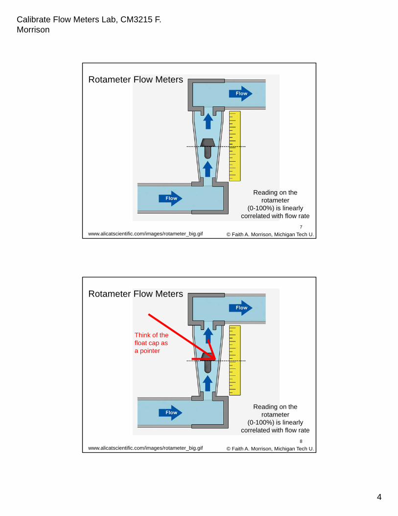
© Faith A. Morrison, Michigan Tech U.www.alicatscientific.com/images/rotameter_big.gif
Rotameter Flow Meters
Reading on the rotameter
(0-100%) is linearly correlated with flow rate
7
© Faith A. Morrison, Michigan Tech U.www.alicatscientific.com/images/rotameter_big.gif
Rotameter Flow Meters
Think of the float cap as a pointer
Reading on the rotameter
(0-100%) is linearly correlated with flow rate
8
Calibrate Flow Meters Lab, CM3215 F. Morrison
5
© Faith A. Morrison, Michigan Tech U.
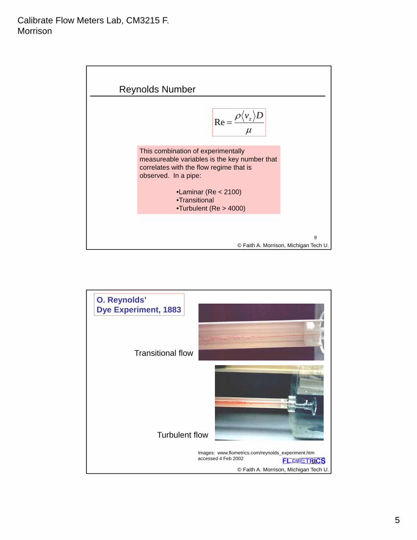
Reynolds Number
DvzRe
This combination of experimentally measureable variables is the key number that correlates with the flow regime that is observed. In a pipe:
•Laminar (Re < 2100)•Transitional•Turbulent (Re > 4000)
9
Images: www.flometrics.com/reynolds_experiment.htmaccessed 4 Feb 2002
Transitional flow
Turbulent flow
O. Reynolds’ Dye Experiment, 1883
© Faith A. Morrison, Michigan Tech U.
10
Calibrate Flow Meters Lab, CM3215 F. Morrison
6
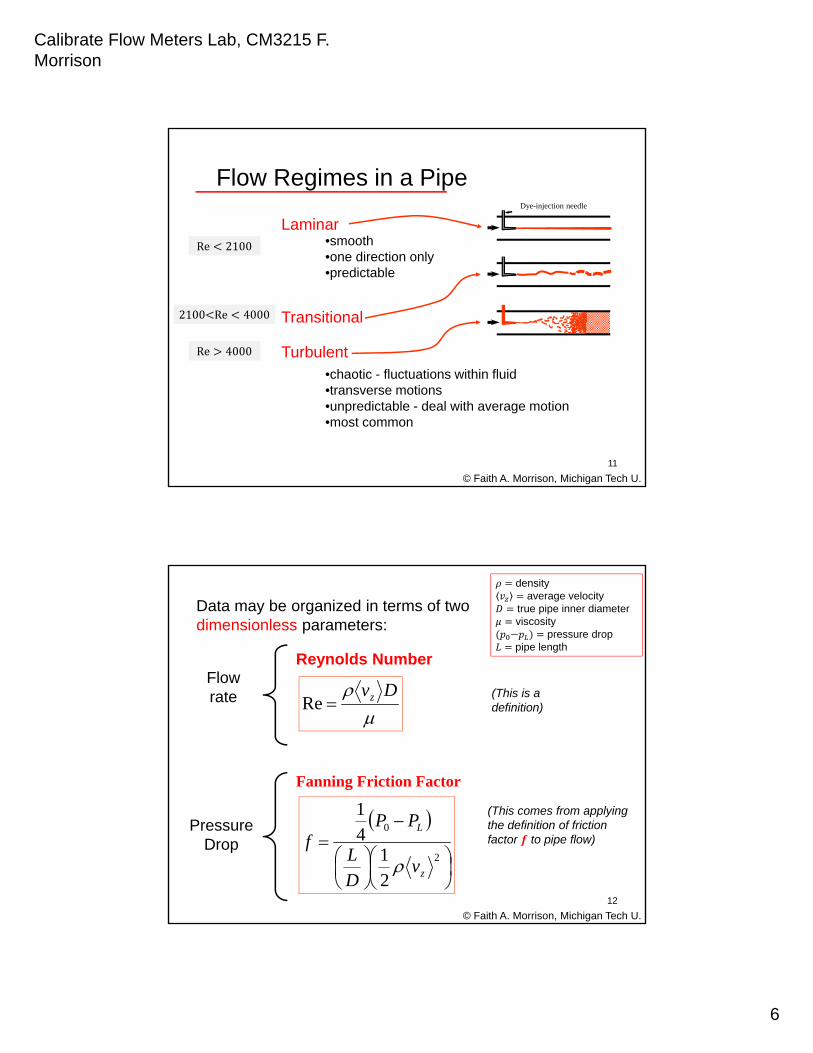
Flow Regimes in a Pipe
Laminar
Transitional
Turbulent
•smooth•one direction only•predictable
•chaotic - fluctuations within fluid•transverse motions•unpredictable - deal with average motion•most common
Dye-injection needle
© Faith A. Morrison, Michigan Tech U.
11
Re 2100
2100 Re 4000
Re 4000
Reynolds Number
© Faith A. Morrison, Michigan Tech U.
Fanning Friction Factor
DvzRe
Flow rate
Pressure Drop
Data may be organized in terms of two dimensionless parameters:
2
0
21
41
z
L
vDL
PPf
12
(This is a definition)
(This comes from applying the definition of friction factor to pipe flow)
densityaverage velocity
true pipe inner diameterviscosity
pressure droppipe length
Calibrate Flow Meters Lab, CM3215 F. Morrison
7
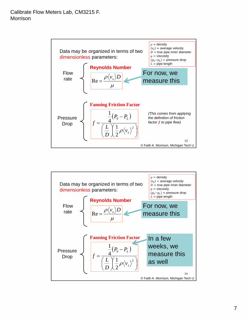
Reynolds Number
© Faith A. Morrison, Michigan Tech U.
Fanning Friction Factor
DvzRe
Flow rate
Pressure Drop
Data may be organized in terms of two dimensionless parameters:
2
0
21
41
z
L
vDL
PPf
13
(This is a definition)
For now, we measure this
densityaverage velocity
true pipe inner diameterviscosity
pressure droppipe length
(This comes from applying the definition of friction factor to pipe flow)
(This comes from applying the definition of friction factor to pipe flow)
In a few weeks, we measure this as well
Reynolds Number
© Faith A. Morrison, Michigan Tech U.
Fanning Friction Factor
DvzRe
Flow rate
Pressure Drop
Data may be organized in terms of two dimensionless parameters:
2
0
21
41
z
L
vDL
PPf
14
densityaverage velocity
true pipe inner diameterviscosity
pressure droppipe length
(This is a definition)
For now, we measure this
Calibrate Flow Meters Lab, CM3215 F. Morrison
8
© Faith A. Morrison, Michigan Tech U.
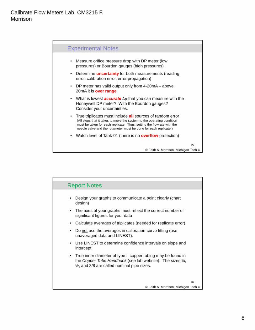
Experimental Notes
• Measure orifice pressure drop with DP meter (low pressures) or Bourdon gauges (high pressures)
• Determine uncertainty for both measurements (reading error, calibration error, error propagation)
• DP meter has valid output only from 4-20mA – above 20mA it is over range
• What is lowest accurate Δ that you can measure with the Honeywell DP meter? With the Bourdon gauges? Consider your uncertainties.
• True triplicates must include all sources of random error (All steps that it takes to move the system to the operating condition must be taken for each replicate. Thus, setting the flowrate with the needle valve and the rotameter must be done for each replicate.)
• Watch level of Tank-01 (there is no overflow protection)
15
© Faith A. Morrison, Michigan Tech U.
Report Notes
• Design your graphs to communicate a point clearly (chart design)
• The axes of your graphs must reflect the correct number of significant figures for your data
• Calculate averages of triplicates (needed for replicate error)
• Do not use the averages in calibration-curve fitting (use unaveraged data and LINEST).
• Use LINEST to determine confidence intervals on slope and intercept
• True inner diameter of type L copper tubing may be found in the Copper Tube Handbook (see lab website). The sizes ¼, ½, and 3/8 are called nominal pipe sizes.
16
Calibrate Flow Meters Lab, CM3215 F. Morrison
9
© Faith A. Morrison, Michigan Tech U.
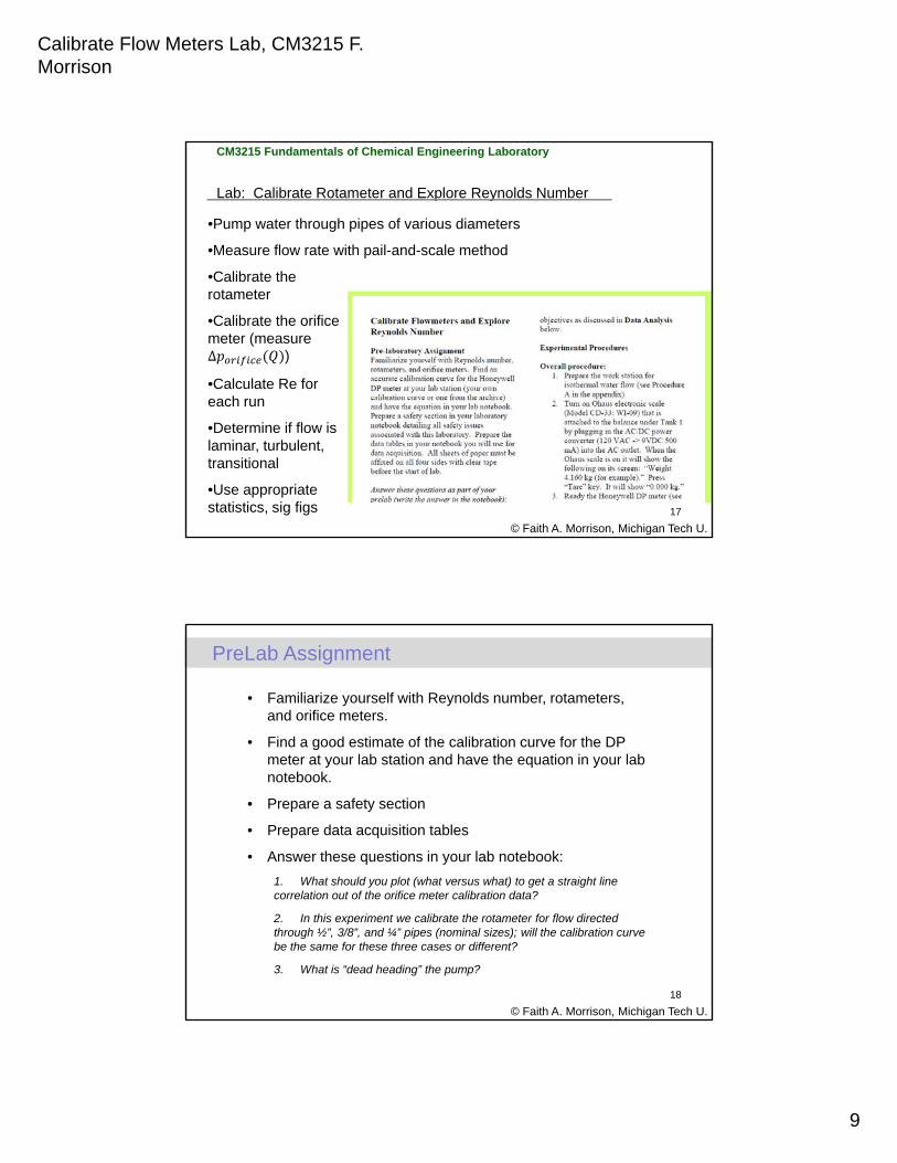
CM3215 Fundamentals of Chemical Engineering Laboratory
Lab: Calibrate Rotameter and Explore Reynolds Number
•Pump water through pipes of various diameters
•Measure flow rate with pail-and-scale method
•Calibrate the rotameter
•Calibrate the orifice meter (measure Δ )
•Calculate Re for each run
•Determine if flow is laminar, turbulent, transitional
•Use appropriate statistics, sig figs 17
© Faith A. Morrison, Michigan Tech U.
PreLab Assignment
• Familiarize yourself with Reynolds number, rotameters, and orifice meters.
• Find a good estimate of the calibration curve for the DP meter at your lab station and have the equation in your lab notebook.
• Prepare a safety section
• Prepare data acquisition tables
• Answer these questions in your lab notebook:
1. What should you plot (what versus what) to get a straight line correlation out of the orifice meter calibration data?
2. In this experiment we calibrate the rotameter for flow directed through ½”, 3/8”, and ¼” pipes (nominal sizes); will the calibration curve be the same for these three cases or different?
3. What is “dead heading” the pump?
18
Calibrate Flow Meters Lab, CM3215 F. Morrison
10
© Faith A. Morrison, Michigan Tech U.
19
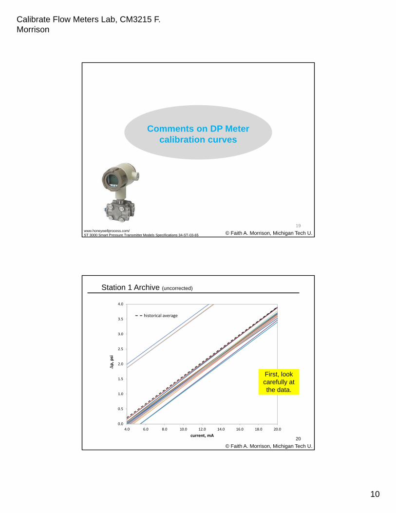
Comments on DP Meter calibration curves
www.honeywellprocess.com/ST 3000 Smart Pressure Transmitter Models Specifications 34-ST-03-65
© Faith A. Morrison, Michigan Tech U.
Station 1 Archive (uncorrected)
0.0
0.5
1.0
1.5
2.0
2.5
3.0
3.5
4.0
4.0 6.0 8.0 10.0 12.0 14.0 16.0 18.0 20.0
p, psi
current, mA
historical average
First, look carefully at the data.
20
Calibrate Flow Meters Lab, CM3215 F. Morrison
11
© Faith A. Morrison, Michigan Tech U.
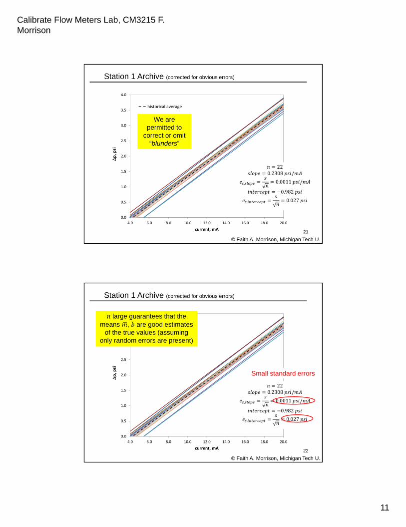
Station 1 Archive (corrected for obvious errors)
0.0
0.5
1.0
1.5
2.0
2.5
3.0
3.5
4.0
4.0 6.0 8.0 10.0 12.0 14.0 16.0 18.0 20.0
p, psi
current, mA
historical average
220.2308 /
, 0.0011 /
0.982
, 0.027
We are permitted to
correct or omit “blunders”
21
© Faith A. Morrison, Michigan Tech U.
Station 1 Archive (corrected for obvious errors)
0.0
0.5
1.0
1.5
2.0
2.5
3.0
3.5
4.0
4.0 6.0 8.0 10.0 12.0 14.0 16.0 18.0 20.0
p, psi
current, mA
historical average
220.2308 /
, 0.0011 /
0.982
, 0.027
large guarantees that the means , are good estimates
of the true values (assuming only random errors are present)
Small standard errors
22
Calibrate Flow Meters Lab, CM3215 F. Morrison
12
0.0
0.5
1.0
1.5
2.0
2.5
3.0
3.5
4.0
4.0 6.0 8.0 10.0 12.0 14.0 16.0 18.0 20.0
p, psi
current, mA
historical average
© Faith A. Morrison, Michigan Tech U.
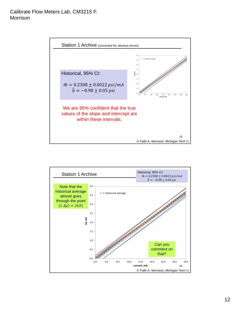
Station 1 Archive (corrected for obvious errors)
Historical, 95% CI:
0.2308 0.0022 /0.98 0.05
We are 95% confident that the true values of the slope and intercept are
within these intervals.
23
0.0
0.5
1.0
1.5
2.0
2.5
3.0
3.5
4.0
4.0 6.0 8.0 10.0 12.0 14.0 16.0 18.0 20.0
p, psi
current, mA
historical average
© Faith A. Morrison, Michigan Tech U.
Station 1 Archive Historical, 95% CI:0.2308 0.0022 /
0.98 0.05
24
Note that the historical average
almost goes through the point
, Δ 4,0
Can you comment on
that?
Calibrate Flow Meters Lab, CM3215 F. Morrison
13
0.0
0.5
1.0
1.5
2.0
2.5
3.0
3.5
4.0
4.0 6.0 8.0 10.0 12.0 14.0 16.0 18.0 20.0
p, psi
current, mA
historical average
© Faith A. Morrison, Michigan Tech U.
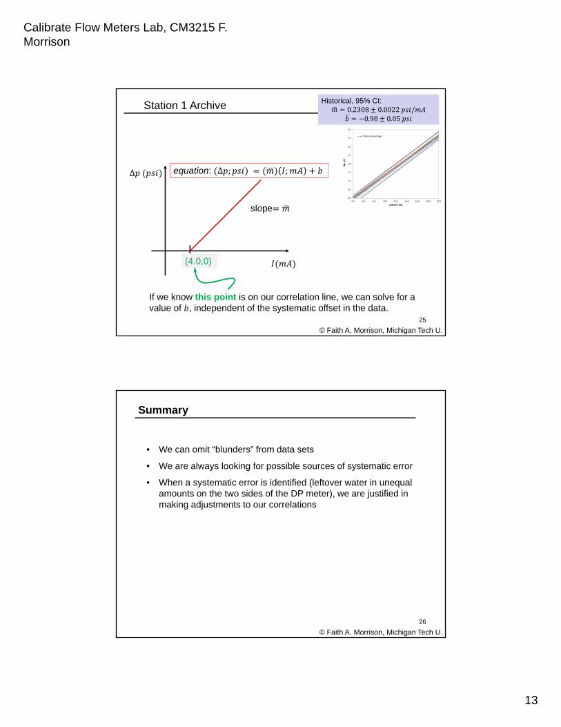
Station 1 Archive Historical, 95% CI:0.2308 0.0022 /
0.98 0.05
25
Δ
(4.0,0)
slope
equation: Δ ; ;
If we know this point is on our correlation line, we can solve for a value of , independent of the systematic offset in the data.
© Faith A. Morrison, Michigan Tech U.
• We can omit “blunders” from data sets
• We are always looking for possible sources of systematic error
• When a systematic error is identified (leftover water in unequal amounts on the two sides of the DP meter), we are justified in making adjustments to our correlations
26
Summary