Calculus III 2
90
-
Upload
iamabdullah -
Category
Documents
-
view
25 -
download
2
description
For downloadings sake!
Transcript of Calculus III 2
Vector-Valued Functions
Calculus-III
Dr. Imran Rashid
Department of Mathematics
COMSATS Institute of Information Technology, Islamabad,
Pakistan
Calculus-III, BCE-III Spring 2013
Vector-Valued Functions
Outline
Vector-Valued Functions
Parametric Curves in 3−SpaceCalculus of Vector-Valued Functions
Change of Parameter; Arc Length
Unit Tangent, Normal, and Binormal Vectors
Curvature
Calculus-III, BCE-III Spring 2013
Vector-Valued Functions
Parametric Curves in 3−SpaceCalculus of Vector-Valued FunctionsChange of Parameter; Arc LengthUnit Tangent, Normal, and Binormal VectorsCurvature
Vector-Valued Functions
Calculus-III, BCE-III Spring 2013
Vector-Valued Functions
Parametric Curves in 3−SpaceCalculus of Vector-Valued FunctionsChange of Parameter; Arc LengthUnit Tangent, Normal, and Binormal VectorsCurvature
Parametric Curves in 3−Space
Calculus-III, BCE-III Spring 2013
Vector-Valued Functions
Parametric Curves in 3−SpaceCalculus of Vector-Valued FunctionsChange of Parameter; Arc LengthUnit Tangent, Normal, and Binormal VectorsCurvature
Overview
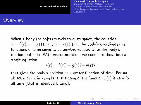
When a body (or objet) travels through space, the equation
x = f (t), y = g(t), and z = h(t) that the body's coordinates as
functions of time serve as parametric equations for the body's
motion and path. With vector notation, we condense these into a
single equation
r(t) = f (t)i+ g(t)j+ h(t)k
that gives the body's position as a vector function of time. For an
object moving in xy−plane, the component function h(t) is zero for
all time (that is, identically zero).
Calculus-III, BCE-III Spring 2013
Vector-Valued Functions
Parametric Curves in 3−SpaceCalculus of Vector-Valued FunctionsChange of Parameter; Arc LengthUnit Tangent, Normal, and Binormal VectorsCurvature
Overview
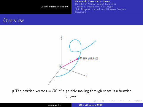
p The position vector r =⇀
OP of a particle moving through space is a function
of time.
Calculus-III, BCE-III Spring 2013
Vector-Valued Functions
Parametric Curves in 3−SpaceCalculus of Vector-Valued FunctionsChange of Parameter; Arc LengthUnit Tangent, Normal, and Binormal VectorsCurvature
Overview
The point (x , y , z) = (f (t), g(t), h(t)), t ∈ I , makes up the curve
in space that we call the particle's path.
The equations
x = f (t), y = g(t), and z = h(t)
parameterize the curve.
A curve in space can also be represented in vector form. The vector
r =⇀OP = f (t)i+ g(t)j+ h(t)k
from the origin to the particle's position P(f (t), g(t), h(t)) at time
t is the particle's position vector.
Calculus-III, BCE-III Spring 2013
Vector-Valued Functions
Parametric Curves in 3−SpaceCalculus of Vector-Valued FunctionsChange of Parameter; Arc LengthUnit Tangent, Normal, and Binormal VectorsCurvature
Overview
The functions f , g , and h are the component functions
(components) of the position vector.
We think of the particle's path as the curve traced by r during the
time interval I .
The equations
x = f (t), y = g(t), and z = h(t)
is a vector function or vector-valued function on a domain set D is
a rule that assigns a vector in space to each element in D.
Calculus-III, BCE-III Spring 2013

Vector-Valued Functions
Parametric Curves in 3−SpaceCalculus of Vector-Valued FunctionsChange of Parameter; Arc LengthUnit Tangent, Normal, and Binormal VectorsCurvature
Graphing Helix
The vector function r(t) = (cos t)i+ (sin t)j+ tk is de�ned for all
real values of t.
The upper half of the helix r = (cos t)i + (sin t)j + tk
Calculus-III, BCE-III Spring 2013
Vector-Valued Functions
Parametric Curves in 3−SpaceCalculus of Vector-Valued FunctionsChange of Parameter; Arc LengthUnit Tangent, Normal, and Binormal VectorsCurvature
Domain of Vector-Valued Function
Example: The component functions of
r(t) = 〈t, t2, t3〉 = ti+ t2j+ t3k
are
x(t) = t, y(t) = t2, z(t) = t3
The domain of r(t) is the set of allowable values for t. If the r(t) isde�ned in terms of component functions and the domain is not
speci�ed explicitly, then it will be understood that the domain is
the intersection of the natural domains of the component functions;
that is called the natural domain of r(t).
Calculus-III, BCE-III Spring 2013
Vector-Valued Functions
Parametric Curves in 3−SpaceCalculus of Vector-Valued FunctionsChange of Parameter; Arc LengthUnit Tangent, Normal, and Binormal VectorsCurvature
Domain of Vector-Valued Function
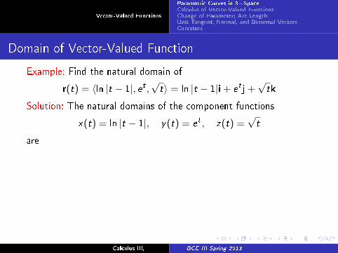
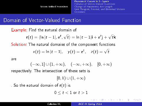
Example: Find the natural domain of
r(t) = 〈ln |t − 1|, et ,√t〉 = ln |t − 1|i+ et j+
√tk
Solution: The natural domains of the component functions
x(t) = ln |t − 1|, y(t) = et , z(t) =√t
are
(−∞, 1] ∪ (1,+∞), (−∞,+∞), [0,+∞)
respectively. The intersection of these sets is
[0, 1) ∪ (1,+∞)
. So the natural domain of r(t) is
0 ≤ t < 1 or t > 1
Calculus-III, BCE-III Spring 2013
Vector-Valued Functions
Parametric Curves in 3−SpaceCalculus of Vector-Valued FunctionsChange of Parameter; Arc LengthUnit Tangent, Normal, and Binormal VectorsCurvature
Domain of Vector-Valued Function
Example: Find the natural domain of
r(t) = 〈ln |t − 1|, et ,√t〉 = ln |t − 1|i+ et j+
√tk
Solution: The natural domains of the component functions
x(t) = ln |t − 1|, y(t) = et , z(t) =√t
are
(−∞, 1] ∪ (1,+∞), (−∞,+∞), [0,+∞)
respectively. The intersection of these sets is
[0, 1) ∪ (1,+∞)
. So the natural domain of r(t) is
0 ≤ t < 1 or t > 1
Calculus-III, BCE-III Spring 2013
Vector-Valued Functions
Parametric Curves in 3−SpaceCalculus of Vector-Valued FunctionsChange of Parameter; Arc LengthUnit Tangent, Normal, and Binormal VectorsCurvature
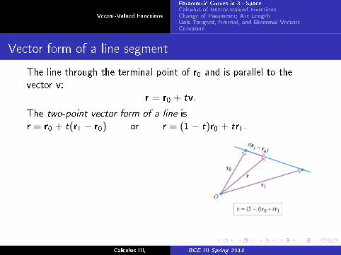
Vector form of a line segment
The line through the terminal point of r0 and is parallel to the
vector v:
r = r0 + tv.
The two-point vector form of a line is
r = r0 + t(r1 − r0) or r = (1− t)r0 + tr1.
The line segment traced from r0 to r1
r = (1− t)r0 + tr1 (0 ≤ t ≤ 1)
Calculus-III, BCE-III Spring 2013
Vector-Valued Functions
Parametric Curves in 3−SpaceCalculus of Vector-Valued FunctionsChange of Parameter; Arc LengthUnit Tangent, Normal, and Binormal VectorsCurvature
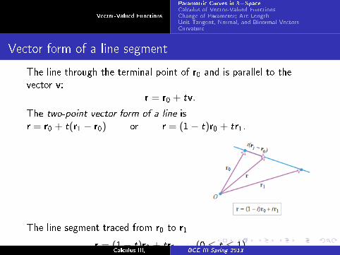
Vector form of a line segment
The line through the terminal point of r0 and is parallel to the
vector v:
r = r0 + tv.
The two-point vector form of a line is
r = r0 + t(r1 − r0) or r = (1− t)r0 + tr1.
The line segment traced from r0 to r1
r = (1− t)r0 + tr1 (0 ≤ t ≤ 1)
Calculus-III, BCE-III Spring 2013
Vector-Valued Functions
Parametric Curves in 3−SpaceCalculus of Vector-Valued FunctionsChange of Parameter; Arc LengthUnit Tangent, Normal, and Binormal VectorsCurvature
Vector form of a line segment
The line through the terminal point of r0 and is parallel to the
vector v:
r = r0 + tv.
The two-point vector form of a line is
r = r0 + t(r1 − r0) or r = (1− t)r0 + tr1.
The line segment traced from r0 to r1
r = (1− t)r0 + tr1 (0 ≤ t ≤ 1)Calculus-III, BCE-III Spring 2013
Vector-Valued Functions
Parametric Curves in 3−SpaceCalculus of Vector-Valued FunctionsChange of Parameter; Arc LengthUnit Tangent, Normal, and Binormal VectorsCurvature
Calculus of Vector-Valued Functions
Calculus-III, BCE-III Spring 2013
Vector-Valued Functions
Parametric Curves in 3−SpaceCalculus of Vector-Valued FunctionsChange of Parameter; Arc LengthUnit Tangent, Normal, and Binormal VectorsCurvature
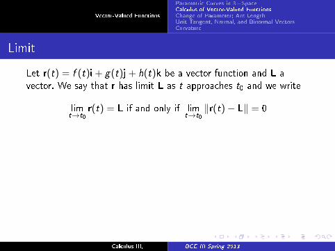
Limit
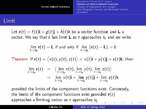
Let r(t) = f (t)i+ g(t)j+ h(t)k be a vector function and L a
vector. We say that r has limit L as t approaches t0 and we write
limt→t0
r(t) = L if and only if limt→t0
‖r(t)− L‖ = 0
Theorem: If r(t) =⟨x(t), y(t), z(t)
⟩= x(t)i+ y(t)j+ z(t)k, then
limt→t0
r(t) =⟨limt→t0
x(t), limt→t0
y(t), limt→t0
z(t)⟩
= limt→t0
x(t)i+ limt→t0
y(t)j+ limt→t0
z(t)k
provided the limits of the component functions exist. Conversely,
the limits of the component functions exist provided r(t)approaches a limiting vector as t approaches t0.
Calculus-III, BCE-III Spring 2013
Vector-Valued Functions
Parametric Curves in 3−SpaceCalculus of Vector-Valued FunctionsChange of Parameter; Arc LengthUnit Tangent, Normal, and Binormal VectorsCurvature
Limit
Let r(t) = f (t)i+ g(t)j+ h(t)k be a vector function and L a
vector. We say that r has limit L as t approaches t0 and we write
limt→t0
r(t) = L if and only if limt→t0
‖r(t)− L‖ = 0
Theorem: If r(t) =⟨x(t), y(t), z(t)
⟩= x(t)i+ y(t)j+ z(t)k, then
limt→t0
r(t) =⟨limt→t0
x(t), limt→t0
y(t), limt→t0
z(t)⟩
= limt→t0
x(t)i+ limt→t0
y(t)j+ limt→t0
z(t)k
provided the limits of the component functions exist. Conversely,
the limits of the component functions exist provided r(t)approaches a limiting vector as t approaches t0.
Calculus-III, BCE-III Spring 2013
Vector-Valued Functions
Parametric Curves in 3−SpaceCalculus of Vector-Valued FunctionsChange of Parameter; Arc LengthUnit Tangent, Normal, and Binormal VectorsCurvature
Continuity
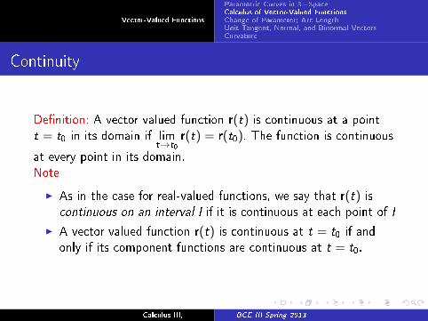
De�nition: A vector valued function r(t) is continuous at a point
t = t0 in its domain if limt→t0
r(t) = r(t0). The function is continuous
at every point in its domain.
Note
I As in the case for real-valued functions, we say that r(t) iscontinuous on an interval I if it is continuous at each point of I
I A vector valued function r(t) is continuous at t = t0 if and
only if its component functions are continuous at t = t0.
Calculus-III, BCE-III Spring 2013
Vector-Valued Functions
Parametric Curves in 3−SpaceCalculus of Vector-Valued FunctionsChange of Parameter; Arc LengthUnit Tangent, Normal, and Binormal VectorsCurvature
Derivative
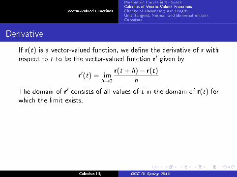
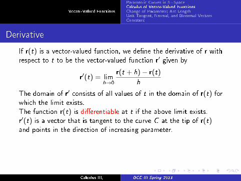
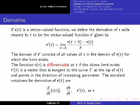
If r(t) is a vector-valued function, we de�ne the derivative of r with
respect to t to be the vector-valued function r′ given by
r′(t) = limh→0
r(t + h)− r(t)
h
The domain of r′ consists of all values of t in the domain of r(t) forwhich the limit exists.
The function r(t) is di�erentiable at t if the above limit exists.
r′(t) is a vector that is tangent to the curve C at the tip of r(t)and points in the direction of increasing parameter. The standard
notations for derivative of r(t) are
d
dt[r(t)],
dr
dt, r′(t), or r
Calculus-III, BCE-III Spring 2013
Vector-Valued Functions
Parametric Curves in 3−SpaceCalculus of Vector-Valued FunctionsChange of Parameter; Arc LengthUnit Tangent, Normal, and Binormal VectorsCurvature
Derivative
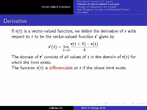
If r(t) is a vector-valued function, we de�ne the derivative of r with
respect to t to be the vector-valued function r′ given by
r′(t) = limh→0
r(t + h)− r(t)
h
The domain of r′ consists of all values of t in the domain of r(t) forwhich the limit exists.
The function r(t) is di�erentiable at t if the above limit exists.
r′(t) is a vector that is tangent to the curve C at the tip of r(t)and points in the direction of increasing parameter.
The standard
notations for derivative of r(t) are
d
dt[r(t)],
dr
dt, r′(t), or r
Calculus-III, BCE-III Spring 2013
Vector-Valued Functions
Parametric Curves in 3−SpaceCalculus of Vector-Valued FunctionsChange of Parameter; Arc LengthUnit Tangent, Normal, and Binormal VectorsCurvature
Derivative
If r(t) is a vector-valued function, we de�ne the derivative of r with
respect to t to be the vector-valued function r′ given by
r′(t) = limh→0
r(t + h)− r(t)
h
The domain of r′ consists of all values of t in the domain of r(t) forwhich the limit exists.
The function r(t) is di�erentiable at t if the above limit exists.
r′(t) is a vector that is tangent to the curve C at the tip of r(t)and points in the direction of increasing parameter. The standard
notations for derivative of r(t) are
d
dt[r(t)],
dr
dt, r′(t), or r
Calculus-III, BCE-III Spring 2013
Vector-Valued Functions
Parametric Curves in 3−SpaceCalculus of Vector-Valued FunctionsChange of Parameter; Arc LengthUnit Tangent, Normal, and Binormal VectorsCurvature
Derivative Geometrically
Calculus-III, BCE-III Spring 2013
Vector-Valued Functions
Parametric Curves in 3−SpaceCalculus of Vector-Valued FunctionsChange of Parameter; Arc LengthUnit Tangent, Normal, and Binormal VectorsCurvature
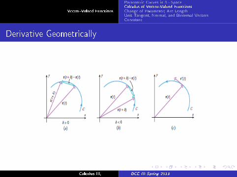
Geometric Interpretation of the Derivative
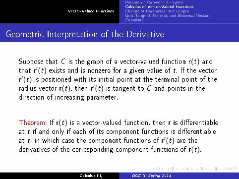
Suppose that C is the graph of a vector-valued function r(t) andthat r′(t) exists and is nonzero for a given value of t. If the vector
r′(t) is positioned with its initial point at the terminal point of the
radius vector r(t), then r′(t) is tangent to C and points in the
direction of increasing parameter.
Theorem: If r(t) is a vector-valued function, then r is di�erentiable
at t if and only if each of its component functions is di�erentiable
at t, in which case the component functions of r′(t) are the
derivatives of the corresponding component functions of r(t).
Calculus-III, BCE-III Spring 2013
Vector-Valued Functions
Parametric Curves in 3−SpaceCalculus of Vector-Valued FunctionsChange of Parameter; Arc LengthUnit Tangent, Normal, and Binormal VectorsCurvature
Geometric Interpretation of the Derivative
Suppose that C is the graph of a vector-valued function r(t) andthat r′(t) exists and is nonzero for a given value of t. If the vector
r′(t) is positioned with its initial point at the terminal point of the
radius vector r(t), then r′(t) is tangent to C and points in the
direction of increasing parameter.
Theorem: If r(t) is a vector-valued function, then r is di�erentiable
at t if and only if each of its component functions is di�erentiable
at t, in which case the component functions of r′(t) are the
derivatives of the corresponding component functions of r(t).
Calculus-III, BCE-III Spring 2013
Vector-Valued Functions
Parametric Curves in 3−SpaceCalculus of Vector-Valued FunctionsChange of Parameter; Arc LengthUnit Tangent, Normal, and Binormal VectorsCurvature
Derivative of a Vector Function
Let u and v be di�erentiable vector functions of t, C a constant
vector, k any scalar, and f any di�erentiable scalar function.
1. Constant Function Ruled
dtC = 0
2. Scalar Multiple Rule
d
dt[ku(t)] = ku′(t)
d
dt[f (t)u(t)] = f ′(t)u(t) + f (t)u′(t)
3. Sum Ruled
dt[u(t) + v(t)] = u′(t) + v′(t)
Calculus-III, BCE-III Spring 2013

Vector-Valued Functions
Parametric Curves in 3−SpaceCalculus of Vector-Valued FunctionsChange of Parameter; Arc LengthUnit Tangent, Normal, and Binormal VectorsCurvature
Derivative Rules
4. Di�erence Rule
d
dt[u(t)− v(t)] = u′(t)− v′(t)
5. Dot Product Rule
d
dt[u(t) · v(t)] = u′(t) · v(t) + u(t) · v′(t)
6. Cross Product Rule
d
dt[u(t)× v(t)] = u′(t)× v(t) + u(t)× v′(t)
7. Chain Ruled
dt[u(f (t))] = f ′(t)u′(f (t))
Calculus-III, BCE-III Spring 2013
Vector-Valued Functions
Parametric Curves in 3−SpaceCalculus of Vector-Valued FunctionsChange of Parameter; Arc LengthUnit Tangent, Normal, and Binormal VectorsCurvature
Tangent Lines
De�nition: Let P be a point on the graph of a vector-valued
function r(t), and let r(t0) be the radius vector from the origin to
P . If r′(t0) exists and r′(t0) 6= 0, then we call r′(t0) a tangent
vector to the graph of r(t) at r(t0), and we call the line through P
that is parallel to the tangent line to the graph of r(t) at r(t0)
The tangent line to the graph of r(t) at r0 is given by
r = r0 + tv0
Calculus-III, BCE-III Spring 2013
Vector-Valued Functions
Parametric Curves in 3−SpaceCalculus of Vector-Valued FunctionsChange of Parameter; Arc LengthUnit Tangent, Normal, and Binormal VectorsCurvature
Tangent Lines
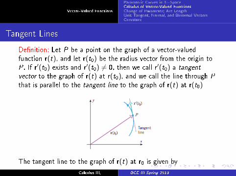
De�nition: Let P be a point on the graph of a vector-valued
function r(t), and let r(t0) be the radius vector from the origin to
P . If r′(t0) exists and r′(t0) 6= 0, then we call r′(t0) a tangent
vector to the graph of r(t) at r(t0), and we call the line through P
that is parallel to the tangent line to the graph of r(t) at r(t0)
The tangent line to the graph of r(t) at r0 is given by
r = r0 + tv0Calculus-III, BCE-III Spring 2013
Vector-Valued Functions
Parametric Curves in 3−SpaceCalculus of Vector-Valued FunctionsChange of Parameter; Arc LengthUnit Tangent, Normal, and Binormal VectorsCurvature
Derivatives of Dot and Cross Products
Theorem: If r(t) is a vector-valued function and ‖r(t)‖ is constantfor all t, then
r(t) · r′(t) = 0
that is , r(t) and r′(t) are orthogonal vectors for all t.
Proof: Asd
dt[r1(t) · r2(t)] = r1(t) ·
dr2
dt+
dr1
dt· r2(t)
It follows with r1 = r2 = r that
d
dt[r(t) · r(t)] = r(t) · dr
dt+
dr
dt· r(t)
d
dt[‖r(t)‖2] = 2r(t) · dr
dt
But ‖r(t)‖2 is constant, so its derivative is zero. Thus
2r(t) · drdt
= 0
Calculus-III, BCE-III Spring 2013
Vector-Valued Functions
Parametric Curves in 3−SpaceCalculus of Vector-Valued FunctionsChange of Parameter; Arc LengthUnit Tangent, Normal, and Binormal VectorsCurvature
Antiderivatives and De�nite Integrals
An antiderivative for a vector-valued function r(t) is avector-valued function R(t) such that
R′(t) = r(t)
Using integral notation∫r(t)dt = R(t) + C
where C represents an arbitrary constant vector.
Like di�erentiation of a vector-valued function, antiderivative is also
performed component wise.
Calculus-III, BCE-III Spring 2013
Vector-Valued Functions
Parametric Curves in 3−SpaceCalculus of Vector-Valued FunctionsChange of Parameter; Arc LengthUnit Tangent, Normal, and Binormal VectorsCurvature
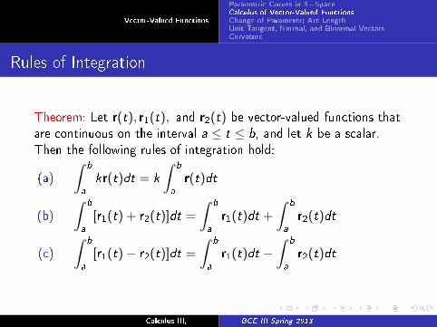
Rules of Integration
Theorem: Let r(t), r1(t), and r2(t) be vector-valued functions that
are continuous on the interval a ≤ t ≤ b, and let k be a scalar.
Then the following rules of integration hold:
(a)
∫b
a
kr(t)dt = k
∫b
a
r(t)dt
(b)
∫b
a
[r1(t) + r2(t)]dt =
∫b
a
r1(t)dt +
∫b
a
r2(t)dt
(c)
∫b
a
[r1(t)− r2(t)]dt =
∫b
a
r1(t)dt −∫
b
a
r2(t)dt
Calculus-III, BCE-III Spring 2013
Vector-Valued Functions
Parametric Curves in 3−SpaceCalculus of Vector-Valued FunctionsChange of Parameter; Arc LengthUnit Tangent, Normal, and Binormal VectorsCurvature
Change of Parameter; Arc Length
Calculus-III, BCE-III Spring 2013
Vector-Valued Functions
Parametric Curves in 3−SpaceCalculus of Vector-Valued FunctionsChange of Parameter; Arc LengthUnit Tangent, Normal, and Binormal VectorsCurvature
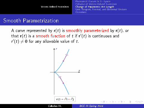
Smooth Parametrization
A curve represented by r(t) is smoothly parameterized by r(t), orthat r(t) is a smooth function of t if r′(t) is continuous andr′(t) 6= 0 for any allowable value of t.
Calculus-III, BCE-III Spring 2013
Vector-Valued Functions
Parametric Curves in 3−SpaceCalculus of Vector-Valued FunctionsChange of Parameter; Arc LengthUnit Tangent, Normal, and Binormal VectorsCurvature
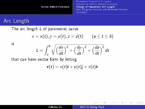
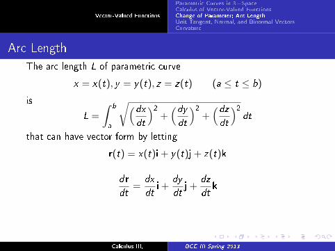
Arc Length
The arc length L of parametric curve
x = x(t), y = y(t), z = z(t) (a ≤ t ≤ b)
is
L =
∫b
a
√(dxdt
)2+(dydt
)2+(dzdt
)2dt
that can have vector form by letting
r(t) = x(t)i+ y(t)j+ z(t)k
dr
dt=
dx
dti+
dy
dtj+
dz
dtk
∥∥∥drdt
∥∥∥ =
√(dxdt
)2+(dydt
)2+(dzdt
)2
Calculus-III, BCE-III Spring 2013
Vector-Valued Functions
Parametric Curves in 3−SpaceCalculus of Vector-Valued FunctionsChange of Parameter; Arc LengthUnit Tangent, Normal, and Binormal VectorsCurvature
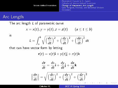
Arc Length
The arc length L of parametric curve
x = x(t), y = y(t), z = z(t) (a ≤ t ≤ b)
is
L =
∫b
a
√(dxdt
)2+(dydt
)2+(dzdt
)2dt
that can have vector form by letting
r(t) = x(t)i+ y(t)j+ z(t)k
dr
dt=
dx
dti+
dy
dtj+
dz
dtk
∥∥∥drdt
∥∥∥ =
√(dxdt
)2+(dydt
)2+(dzdt
)2Calculus-III, BCE-III Spring 2013
Vector-Valued Functions
Parametric Curves in 3−SpaceCalculus of Vector-Valued FunctionsChange of Parameter; Arc LengthUnit Tangent, Normal, and Binormal VectorsCurvature
Arc Length
Theorem: If C is the graph of a smooth vector-valued function r(t),then its arc length L from t = a to t = b is
L =
∫b
a
∥∥∥drdt
∥∥∥ dt
Calculus-III, BCE-III Spring 2013
Vector-Valued Functions
Parametric Curves in 3−SpaceCalculus of Vector-Valued FunctionsChange of Parameter; Arc LengthUnit Tangent, Normal, and Binormal VectorsCurvature
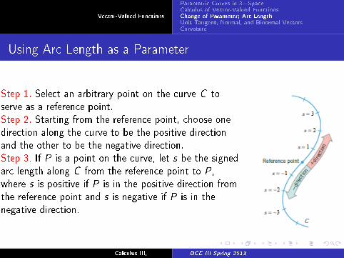
Using Arc Length as a Parameter
Step 1. Select an arbitrary point on the curve C to
serve as a reference point.
Step 2. Starting from the reference point, choose one
direction along the curve to be the positive direction
and the other to be the negative direction.
Step 3. If P is a point on the curve, let s be the signed
arc length along C from the reference point to P ,
where s is positive if P is in the positive direction from
the reference point and s is negative if P is in the
negative direction.
Calculus-III, BCE-III Spring 2013
Vector-Valued Functions
Parametric Curves in 3−SpaceCalculus of Vector-Valued FunctionsChange of Parameter; Arc LengthUnit Tangent, Normal, and Binormal VectorsCurvature
Using Arc Length as a Parameter
A parametric representation of a curve with arc length as the
parameter is called an arc length parametrization of the curve.
Note that a given curve will generally have in�nitely many di�erent
arc length parameterizations, since the reference point and
orientation can be chosen arbitrarily.
Calculus-III, BCE-III Spring 2013
Vector-Valued Functions
Parametric Curves in 3−SpaceCalculus of Vector-Valued FunctionsChange of Parameter; Arc LengthUnit Tangent, Normal, and Binormal VectorsCurvature
Using Arc Length as a Parameter
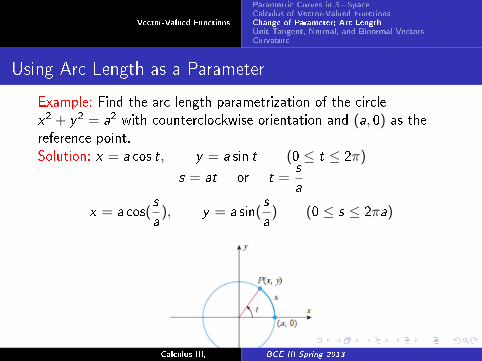
Example: Find the arc length parametrization of the circle
x2 + y2 = a2 with counterclockwise orientation and (a, 0) as thereference point.
Solution: x = a cos t, y = a sin t (0 ≤ t ≤ 2π)
s = at or t =s
a
x = a cos(s
a), y = a sin(
s
a) (0 ≤ s ≤ 2πa)
Calculus-III, BCE-III Spring 2013
Vector-Valued Functions
Parametric Curves in 3−SpaceCalculus of Vector-Valued FunctionsChange of Parameter; Arc LengthUnit Tangent, Normal, and Binormal VectorsCurvature
Change of Parameter
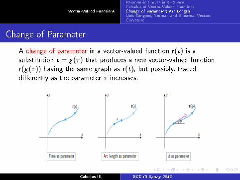
A change of parameter in a vector-valued function r(t) is asubstitution t = g(τ) that produces a new vector-valued function
r(g(τ)) having the same graph as r(t), but possibly, traceddi�erently as the parameter τ increases.
Calculus-III, BCE-III Spring 2013
Vector-Valued Functions
Parametric Curves in 3−SpaceCalculus of Vector-Valued FunctionsChange of Parameter; Arc LengthUnit Tangent, Normal, and Binormal VectorsCurvature
Change of Parameter
A change of parameter in a vector-valued function r(t) is asubstitution t = g(τ) that produces a new vector-valued function
r(g(τ)) having the same graph as r(t), but possibly, traceddi�erently as the parameter τ increases.
Calculus-III, BCE-III Spring 2013
Vector-Valued Functions
Parametric Curves in 3−SpaceCalculus of Vector-Valued FunctionsChange of Parameter; Arc LengthUnit Tangent, Normal, and Binormal VectorsCurvature
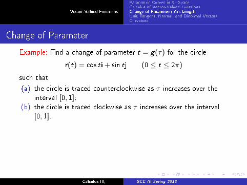
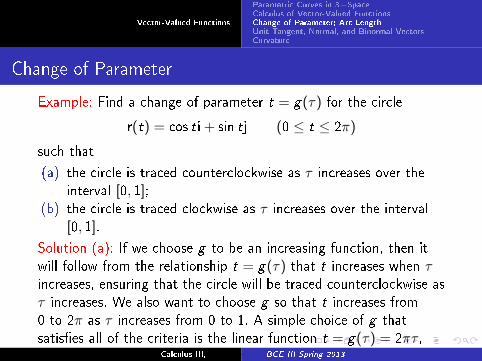
Change of Parameter
Example: Find a change of parameter t = g(τ) for the circle
r(t) = cos ti+ sin tj (0 ≤ t ≤ 2π)
such that
(a) the circle is traced counterclockwise as τ increases over the
interval [0, 1];(b) the circle is traced clockwise as τ increases over the interval
[0, 1].
Solution (a): If we choose g to be an increasing function, then it
will follow from the relationship t = g(τ) that t increases when τincreases, ensuring that the circle will be traced counterclockwise as
τ increases. We also want to choose g so that t increases from
0 to 2π as τ increases from 0 to 1. A simple choice of g that
satis�es all of the criteria is the linear function t = g(τ) = 2πτ ,which is the desired change of parameter.
Calculus-III, BCE-III Spring 2013
Vector-Valued Functions
Parametric Curves in 3−SpaceCalculus of Vector-Valued FunctionsChange of Parameter; Arc LengthUnit Tangent, Normal, and Binormal VectorsCurvature
Change of Parameter
Example: Find a change of parameter t = g(τ) for the circle
r(t) = cos ti+ sin tj (0 ≤ t ≤ 2π)
such that
(a) the circle is traced counterclockwise as τ increases over the
interval [0, 1];(b) the circle is traced clockwise as τ increases over the interval
[0, 1].
Solution (a): If we choose g to be an increasing function, then it
will follow from the relationship t = g(τ) that t increases when τincreases, ensuring that the circle will be traced counterclockwise as
τ increases. We also want to choose g so that t increases from
0 to 2π as τ increases from 0 to 1. A simple choice of g that
satis�es all of the criteria is the linear function t = g(τ) = 2πτ ,which is the desired change of parameter.Calculus-III, BCE-III Spring 2013
Vector-Valued Functions
Parametric Curves in 3−SpaceCalculus of Vector-Valued FunctionsChange of Parameter; Arc LengthUnit Tangent, Normal, and Binormal VectorsCurvature
Change of Parameter
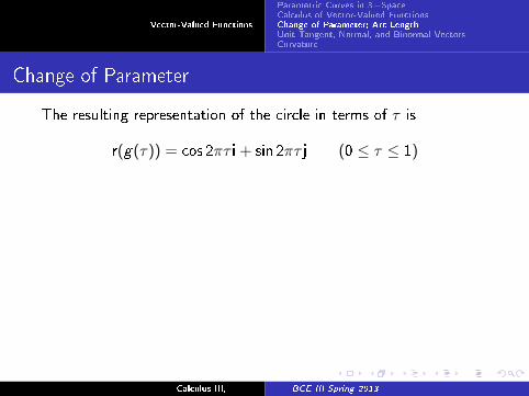
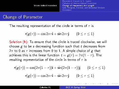
The resulting representation of the circle in terms of τ is
r(g(τ)) = cos 2πτ i+ sin 2πτ j (0 ≤ τ ≤ 1)
Solution (b): To ensure that the circle is traced clockwise, we will
choose g to be a decreasing function such that t decreases from
2π to 0 as τ increases from 0 to 1. A simple choice of g that
achieves this is the linear function t = g(τ) = 2π(1− τ). Theresulting representation of the circle in terms of τ is
r(g(τ)) = cos(2π(1− τ))i+ sin(2π(1− τ))j (0 ≤ τ ≤ 1)
r(g(τ)) = cos 2πτ i− sin 2πτ j (0 ≤ τ ≤ 1)
Calculus-III, BCE-III Spring 2013
Vector-Valued Functions
Parametric Curves in 3−SpaceCalculus of Vector-Valued FunctionsChange of Parameter; Arc LengthUnit Tangent, Normal, and Binormal VectorsCurvature
Change of Parameter
When making a change of parameter t = g(τ) in a vector-valued
function r(t), it will be important to ensure that the new
vector-valued function r(g(τ)) is smooth if r(t) is smooth. The
following theorem establishes the condition under which it happens.
Theorem (Chain Rule): Let r(t) be a vector-valued function that is
di�erentiable with respect to t. If t = g(τ) is a change of
parameter in which g is di�erentiable with respect to τ , thenr(g(τ)) is di�erentiable with respect to τ and
dr
dτ=
dr
dt
dt
dτ
Calculus-III, BCE-III Spring 2013
Vector-Valued Functions
Parametric Curves in 3−SpaceCalculus of Vector-Valued FunctionsChange of Parameter; Arc LengthUnit Tangent, Normal, and Binormal VectorsCurvature
Change of Parameter
A change of parameter t = g(τ) in which r(g(τ)) is smooth if r(t)is smooth is called a smooth change of parameter.
It follows that t = g(τ) will be a smooth change of parameter if dt
dτ
is continuous and dt
dτ 6= 0 for all values of τ , since these conditions
imply that dr
dτ is continuous and nonzero if dr
dtis continuous and
nonzero.
→ If dt
dτ > 0 for all τ then it is a positive change of parameter.
→ If dt
dτ < 0 for all τ then it is a negative change of parameter.
A positive change of parameter preserves the orientation of a
parametric curve, and a negative change of parameter reverses it.
Calculus-III, BCE-III Spring 2013
Vector-Valued Functions
Parametric Curves in 3−SpaceCalculus of Vector-Valued FunctionsChange of Parameter; Arc LengthUnit Tangent, Normal, and Binormal VectorsCurvature
Finding Arc Length Parameterizations
Theorem: Let C be the graph of a smooth vector-valued function
r(t) and let r(t0) be any point on C . Then the following formula
de�nes a positive change of parameter from t to s, where s is an
arc length parameter having r(t0) as its reference point
s =
∫t
t0
∥∥∥drdu
∥∥∥ duIn component form
s =
∫t
t0
√(dxdu
)2+(dydu
)2+(dzdu
)2du
Calculus-III, BCE-III Spring 2013
Vector-Valued Functions
Parametric Curves in 3−SpaceCalculus of Vector-Valued FunctionsChange of Parameter; Arc LengthUnit Tangent, Normal, and Binormal VectorsCurvature
Finding Arc Length Parameterizations
Example: Find the arc length parametrization of the circular helix
r = cos ti+ sin tj+ tk
that has reference point r(0) = (1, 0, 0) and the same orientation as
the given helix.
Example: A bug walks along the trunk of a tree following a path
modeled by the circular helix in last example. The bug starts at the
reference point (1, 0, 0) and walks up the helix for a distance of 10
units. what are the bug's �al coordinates?
Calculus-III, BCE-III Spring 2013
Vector-Valued Functions
Parametric Curves in 3−SpaceCalculus of Vector-Valued FunctionsChange of Parameter; Arc LengthUnit Tangent, Normal, and Binormal VectorsCurvature
Properties of Arc Length Parameterizations
Theorem:
(a) If C is the graph of a smooth vector-valued function r(t), wheret is a general parameter, and if s is the arc length parameter for C
de�ned by formula above, then for every value of t the tangent
vector has length ∥∥∥drdt
∥∥∥ =ds
dt
(b) If C is the graph of a smooth vector-valued function r(s),where s is an arc length parameter, then for every value of s the
tangent vector to C has length∥∥∥drds
∥∥∥ = 1
Calculus-III, BCE-III Spring 2013
Vector-Valued Functions
Parametric Curves in 3−SpaceCalculus of Vector-Valued FunctionsChange of Parameter; Arc LengthUnit Tangent, Normal, and Binormal VectorsCurvature
Properties of Arc Length Parameterizations
(c) If C is the graph of a smooth vector-valued function r(t), and if∥∥∥drdt
∥∥∥ = 1
for every value of t, then for any value of t0 in the domain of r, the
parameter s = t − t0 is an arc length parameter that has its
reference point at the point on C where t = t0.
Calculus-III, BCE-III Spring 2013
Vector-Valued Functions
Parametric Curves in 3−SpaceCalculus of Vector-Valued FunctionsChange of Parameter; Arc LengthUnit Tangent, Normal, and Binormal VectorsCurvature
Unit Tangent, Normal, and Binormal Vectors
Calculus-III, BCE-III Spring 2013
Vector-Valued Functions
Parametric Curves in 3−SpaceCalculus of Vector-Valued FunctionsChange of Parameter; Arc LengthUnit Tangent, Normal, and Binormal VectorsCurvature
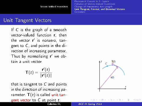
Unit Tangent Vectors
If C is the graph of a smooth
vector-valued function r, then
the vector r′ is nonzero, tan-
gent to C , and points in the di-
rection of increasing parameter.
Thus by normalizing r′ we ob-
tain a unit vector
T(t) =r′(t)
‖r′(t)‖
that is tangent to C and points
in the direction of increasing pa-
rameter. T(t) is called unit tan-
gent vector to C at point t.Calculus-III, BCE-III Spring 2013
Vector-Valued Functions
Parametric Curves in 3−SpaceCalculus of Vector-Valued FunctionsChange of Parameter; Arc LengthUnit Tangent, Normal, and Binormal VectorsCurvature
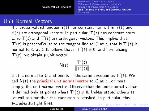
Unit Normal VectorsIf a vector-valued function r(t) has constant norm, then r(t) andr′(t) are orthogonal vectors. In particular, T(t) has constant norm1, so T(t) and T′(t) are orthogonal vectors. This implies that
T′(t) is perpendicular to the tangent line to C at t, that is T′(t) isnormal to C at t. It follows that if T′(t) 6= 0, and normalizing
T′(t), we obtain a unit vector
N(t) =T′(t)
‖T′(t)‖that is normal to C and points in the same direction as T′(t). We
call N(t) the principal unit normal vector to C at t , or more
simply, the unit normal vector. Observe that the unit normal vector
is de�ned only at points where T′(t) 6= 0. Unless stated otherwise,
we will assume that this condition is satis�ed. In particular, this
excludes straight lines.Calculus-III, BCE-III Spring 2013
Vector-Valued Functions
Parametric Curves in 3−SpaceCalculus of Vector-Valued FunctionsChange of Parameter; Arc LengthUnit Tangent, Normal, and Binormal VectorsCurvature
T and N for curves parameterized by arc length
In case where r(s) is parameterized by arc length, we compute of
unit tangent T(s) and the unit normal vector N(s) as:
T(s) = r′(s)
N(s) =r′′(s)
‖r′′(s)‖
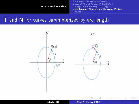
Example: The circle of radius a with counterclockwise orientation
and centered at the origin can be represented by the vector-valued
function
r = a cos ti+ a sin tj (0 ≤ t ≤ 2π)
Parameterize this circle by arc length and �nd T(s) and N(s).
Calculus-III, BCE-III Spring 2013
Vector-Valued Functions
Parametric Curves in 3−SpaceCalculus of Vector-Valued FunctionsChange of Parameter; Arc LengthUnit Tangent, Normal, and Binormal VectorsCurvature
T and N for curves parameterized by arc length
In case where r(s) is parameterized by arc length, we compute of
unit tangent T(s) and the unit normal vector N(s) as:
T(s) = r′(s)
N(s) =r′′(s)
‖r′′(s)‖Example: The circle of radius a with counterclockwise orientation
and centered at the origin can be represented by the vector-valued
function
r = a cos ti+ a sin tj (0 ≤ t ≤ 2π)
Parameterize this circle by arc length and �nd T(s) and N(s).
Calculus-III, BCE-III Spring 2013
Vector-Valued Functions
Parametric Curves in 3−SpaceCalculus of Vector-Valued FunctionsChange of Parameter; Arc LengthUnit Tangent, Normal, and Binormal VectorsCurvature
T and N for curves parameterized by arc length
Calculus-III, BCE-III Spring 2013
Vector-Valued Functions
Parametric Curves in 3−SpaceCalculus of Vector-Valued FunctionsChange of Parameter; Arc LengthUnit Tangent, Normal, and Binormal VectorsCurvature
Binormal Vectors in 3−Space
If C is the graph of a vector-valued function r(t) in 3-space, then
we de�ne the binormal vector to C at t to be
B(t) = T(t)×N(t)
It follows from properties of the cross product that B(t) isorthogonal to both T(t) and N(t) and is oriented relative to T(t)and N(t) by the right-hand rule.
Moreover, T(t)×N(t) is a unit vector since
‖T(t)×N(t)‖ = ‖T(t)‖ ‖N(t)‖ sin(π2) = 1
Thus, {T(t),N(t),B(t)} is a set of three mutually orthogonal unit
vectors.
Calculus-III, BCE-III Spring 2013
Vector-Valued Functions
Parametric Curves in 3−SpaceCalculus of Vector-Valued FunctionsChange of Parameter; Arc LengthUnit Tangent, Normal, and Binormal VectorsCurvature
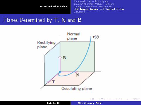
Planes Determined by T, N and B
Calculus-III, BCE-III Spring 2013
Vector-Valued Functions
Parametric Curves in 3−SpaceCalculus of Vector-Valued FunctionsChange of Parameter; Arc LengthUnit Tangent, Normal, and Binormal VectorsCurvature
Coordinate Sysytem Determined by T, N and B
The coordinate system determined by T(t),N(t), and B(t) isright-handed in the sense that each of these vectors is related to
the other two by the right-hand rule:
B(t) = T(t)×N(t), N(t) = B(t)×T(t), T(t) = N(t)× B(t)
This coordinate system is called the TNB-frame or sometimes the
Frenet frame in honor of the French mathematician Jean Frederic
Frenet (1816− 1900) who pioneered its application to the study of
space curves.
Typically, the xyz−coordinate system determined by the unit
vectors i, j, and k remains �xed, whereas the TNB−frame changes
as its origin moves along the curve C .
Calculus-III, BCE-III Spring 2013
Vector-Valued Functions
Parametric Curves in 3−SpaceCalculus of Vector-Valued FunctionsChange of Parameter; Arc LengthUnit Tangent, Normal, and Binormal VectorsCurvature
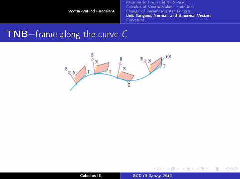
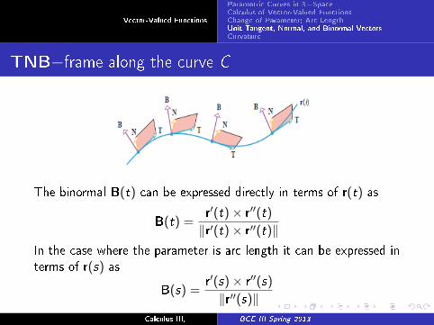
TNB−frame along the curve C
The binormal B(t) can be expressed directly in terms of r(t) as
B(t) =r′(t)× r′′(t)
‖r′(t)× r′′(t)‖In the case where the parameter is arc length it can be expressed in
terms of r(s) as
B(s) =r′(s)× r′′(s)
‖r′′(s)‖
Calculus-III, BCE-III Spring 2013
Vector-Valued Functions
Parametric Curves in 3−SpaceCalculus of Vector-Valued FunctionsChange of Parameter; Arc LengthUnit Tangent, Normal, and Binormal VectorsCurvature
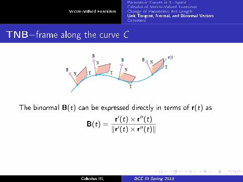
TNB−frame along the curve C
The binormal B(t) can be expressed directly in terms of r(t) as
B(t) =r′(t)× r′′(t)
‖r′(t)× r′′(t)‖
In the case where the parameter is arc length it can be expressed in
terms of r(s) as
B(s) =r′(s)× r′′(s)
‖r′′(s)‖
Calculus-III, BCE-III Spring 2013
Vector-Valued Functions
Parametric Curves in 3−SpaceCalculus of Vector-Valued FunctionsChange of Parameter; Arc LengthUnit Tangent, Normal, and Binormal VectorsCurvature
TNB−frame along the curve C
The binormal B(t) can be expressed directly in terms of r(t) as
B(t) =r′(t)× r′′(t)
‖r′(t)× r′′(t)‖In the case where the parameter is arc length it can be expressed in
terms of r(s) as
B(s) =r′(s)× r′′(s)
‖r′′(s)‖Calculus-III, BCE-III Spring 2013
Vector-Valued Functions
Parametric Curves in 3−SpaceCalculus of Vector-Valued FunctionsChange of Parameter; Arc LengthUnit Tangent, Normal, and Binormal VectorsCurvature
Curvature
Calculus-III, BCE-III Spring 2013
Vector-Valued Functions
Parametric Curves in 3−SpaceCalculus of Vector-Valued FunctionsChange of Parameter; Arc LengthUnit Tangent, Normal, and Binormal VectorsCurvature
What is Curvature
Calculus-III, BCE-III Spring 2013
Vector-Valued Functions
Parametric Curves in 3−SpaceCalculus of Vector-Valued FunctionsChange of Parameter; Arc LengthUnit Tangent, Normal, and Binormal VectorsCurvature
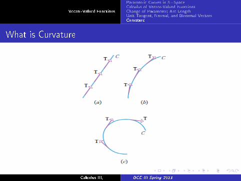
What is Curvature
De�nition: If C is a smooth curve in 2-space or 3-space that is
parameterized by arc length, then the curvature of C , denoted by
κ = κ(s) (κ is Greek �kappa�), is de�ned by
κ(s) =∥∥∥dTds
∥∥∥ = ‖r′′(s)‖
Observe that κ(s) is a real-valued function of s, since it is the
length of dT
dsthat measures the curvature. In general, the curvature
will vary from point to point along a curve.
Example: Show that the circle of radius a parameterized by arc
length
r(s) = a cos( sa
)i+ a sin
( sa
)j (0 ≤ s ≤ 2πa)
has a constant curvature.
Calculus-III, BCE-III Spring 2013
Vector-Valued Functions
Parametric Curves in 3−SpaceCalculus of Vector-Valued FunctionsChange of Parameter; Arc LengthUnit Tangent, Normal, and Binormal VectorsCurvature
What is Curvature
De�nition: If C is a smooth curve in 2-space or 3-space that is
parameterized by arc length, then the curvature of C , denoted by
κ = κ(s) (κ is Greek �kappa�), is de�ned by
κ(s) =∥∥∥dTds
∥∥∥ = ‖r′′(s)‖
Observe that κ(s) is a real-valued function of s, since it is the
length of dT
dsthat measures the curvature. In general, the curvature
will vary from point to point along a curve.
Example: Show that the circle of radius a parameterized by arc
length
r(s) = a cos( sa
)i+ a sin
( sa
)j (0 ≤ s ≤ 2πa)
has a constant curvature.Calculus-III, BCE-III Spring 2013
Vector-Valued Functions
Parametric Curves in 3−SpaceCalculus of Vector-Valued FunctionsChange of Parameter; Arc LengthUnit Tangent, Normal, and Binormal VectorsCurvature
Formulas for Curvature
Theorem: If r(t) is a smooth vector-valued function in 2-space or
3-space, then for each value of t at which T′(t) and r′′(t) exist, thecurvature κ can be expressed as
(a) κ(t) =‖T′(t)‖‖r′(t)‖
(b) κ(t) =‖r′(t)× r′′(t)‖‖r′(t)‖3
Example: Find κ(t) for the circular helix
x = a cos t, y = a sin t, z = ct ; where a > 0.
Calculus-III, BCE-III Spring 2013
Vector-Valued Functions
Parametric Curves in 3−SpaceCalculus of Vector-Valued FunctionsChange of Parameter; Arc LengthUnit Tangent, Normal, and Binormal VectorsCurvature
Formulas for Curvature
Theorem: If r(t) is a smooth vector-valued function in 2-space or
3-space, then for each value of t at which T′(t) and r′′(t) exist, thecurvature κ can be expressed as
(a) κ(t) =‖T′(t)‖‖r′(t)‖
(b) κ(t) =‖r′(t)× r′′(t)‖‖r′(t)‖3
Example: Find κ(t) for the circular helix
x = a cos t, y = a sin t, z = ct ; where a > 0.
Calculus-III, BCE-III Spring 2013
Vector-Valued Functions
Thank you for attention!
Calculus-III, BCE-III Spring 2013