Calculix FEA Beam Part 1: Buliding Geometry and Meshing · Calculix FEA Beam Part 1: Buliding...
53
Homework 6.3: Problem Statement: Reproduce all steps in tutorial by Beede Solution: All steps were followed and completed in the tutorial. The tutorials are linked here individually: http://en.wikiversity.org/wiki/User:Eml5526.s11/Finite_element_analysis The following is the tutorial from http://mechanicalhacks.wordpress.com : Calculix FEA Beam Part 1: Buliding Geometry and Meshing This article is the first segment of several related to CalculiX. This magnum opus of open source is a full non-linear finite element package running on linux, windows, and mac. It is divided into two primary programs, cgx and ccx. The first of the two Calculix GraphiX, cgx, handles pre-processing to define a geometry, mesh, loads, and boundary conditions. The second program Calculix CrunchiX, ccx, handles the number crunching. It will solve for the solution using the finite element method. Then the results will be post-processed using cgx. This tutorial examines the basic usage of cgx to define a beam geometry and mesh. If you’ve already got bConverged installed go ahead and open the SciTE text editor, then “save as” a blank file with name beam.fbd. Saving a blank document with the correct file extension allows SciTE to recognize it and apply the bConverged customizations like source highlights and starting the cgx or ccx program from within the text editor. Its analogous to using an IDE like eclipse to write code. Firing up cgx with the current file as input is available from the Tools->Pre Process menu item or the F10 key. In the case that you’re on a box without bConverged the steps to create an .fbd file are essentially the same on linux or from a dos/cygwin bash shell on windows. Use your favorite text editor to create the .fbd file and then read it using the following command, cgx -b filename.fbd. If you’re on bConverged with windows calling it from the command line add .bat to the end of the cgx command name and make sure you’ve got it in your path. Add the following text to the beam.fbd file as shown in the image below. This is the start of a cgx batch file. Geometry can be created interactively with cgx running or described
Transcript of Calculix FEA Beam Part 1: Buliding Geometry and Meshing · Calculix FEA Beam Part 1: Buliding...

Homework 6.3:
Problem Statement:
Reproduce all steps in tutorial by Beede
Solution:
All steps were followed and completed in the tutorial.
The tutorials are linked here individually:
http://en.wikiversity.org/wiki/User:Eml5526.s11/Finite_element_analysis
The following is the tutorial from http://mechanicalhacks.wordpress.com :
Calculix FEA Beam Part 1: Buliding Geometry and Meshing
This article is the first segment of several related to CalculiX. This magnum opus of
open source is a full non-linear finite element package running on linux, windows, and
mac. It is divided into two primary programs, cgx and ccx. The first of the two Calculix
GraphiX, cgx, handles pre-processing to define a geometry, mesh, loads, and boundary
conditions. The second program Calculix CrunchiX, ccx, handles the number
crunching. It will solve for the solution using the finite element method. Then the
results will be post-processed using cgx. This tutorial examines the basic usage of cgx to
define a beam geometry and mesh.
If you’ve already got bConverged installed go ahead and open the SciTE text editor, then
“save as” a blank file with name beam.fbd. Saving a blank document with the correct file
extension allows SciTE to recognize it and apply the bConverged customizations like
source highlights and starting the cgx or ccx program from within the text editor. Its
analogous to using an IDE like eclipse to write code. Firing up cgx with the current file
as input is available from the Tools->Pre Process menu item or the F10 key.
In the case that you’re on a box without bConverged the steps to create an .fbd file are
essentially the same on linux or from a dos/cygwin bash shell on windows. Use your
favorite text editor to create the .fbd file and then read it using the following
command, cgx -b filename.fbd. If you’re on bConverged with windows calling it from
the command line add .bat to the end of the cgx command name and make sure you’ve
got it in your path.
Add the following text to the beam.fbd file as shown in the image below. This is the start
of a cgx batch file. Geometry can be created interactively with cgx running or described

in a.fbd batch file which is read into cgx at startup. Generally speaking it is easier to
define geometry with a batch file. All the commands are exactly the same between batch
and interactive mode. Interactive mode is a bit more useful when it comes to working
with the mesh like assigning boundary conditions, loads, and constraints to a set of
specific nodes. The first two lines of the batch file define points in cgx model space. The
first point is named p1 located at (x,y,z) = 0. The third line of code defines a cgx line
with name l1 that starts at point p1 and ends a point p2 and has a division of 25
If you’re using bConverged on windows the SciTE editor is configured to launch the cgx
program and feed it the currently active tab, in our case beam.fbd. Just hit the F10 Key
or choose Tools->Pre Process from the menu. The following result is displayed in the
below image. This is the cgx program up and running with the results of the batch file
shown in the graphics area. The keyboard is used to provide most of the commands to
cgx while it is running, also known as interactive mode. In addition the window is
divided into two distinct areas. On the right side top corner is the graphics display area
bordered by a thin black line. Inside the graphics display area clicking and holding the
mouse has the following functionality
1. Left mouse button = rotate
2. Middle mouse button = zoom
3. Right mouse button = pan
Moving the mouse out of the area surrounded by the thin black border the mouse has
different functionality. In this area the left mouse button is used to bring up a menu
which gives the user a graphical front end to some of the cgx commands which can
alternatively be typed on the keyboard. Only a small subset of the commands are
available through the pop up menu.

Now lets expand a bit on the idea of making a simple 100 x 10 x 1 rectangular beam
meshed with 1x1x1 cubes.

In the image above, several more points and line segments have been defined along the
x direction. These extra segments will allow for meshing at the desired resolution of
1x1x1 size elements. The reason for this is that each line segment is internally limited to
99 divisions. It won’t limit the user’s ability to choose an arbitrarily fine mesh, however,
it will require a bit of planning ahead to ensure enough line segments are used to
achieve the necessary mesh resolution. In addition quadratic elements mesh at a
resolution of 2 line divisions equals 1 mesh element side length. Linear elements mesh
at a rate of 1 division equals 1 mesh element length.

In the above image you will also notice the SciTE screen is split down the middle with an
input/output window on the right hand side. This split happens automatically when
using SciTE to launch cgx or ccx. It can be manually turned on or off using the View-
>Outputmenu item. This window is capturing all the cgx program output and keyboard
input. While the cgx window is the active window any keyboard input will be shown on
the bottom line of the output window. In the case of the view above I’ve typed the plot
pa allcommand but have yet to hit the enter button in order to activate it.
The above image shows the results of two commands. plot pa all tells cgx to display all
points p with their names a. More specifically it displays all the points contained within
the cgx set named all. Users can define their own sets with arbitrary members to
manage the problem definition and processing. The second command plus la all is

used to add the lines with their names to the existing plot. If instead plot la all had
been typed after the first command the points and their names would have been
eliminated from the new plot view. It would have redrawn the plot rather than just
including additional information to the existing plot. There is a corresponding minus
command to remove information.
Next, build a surface from the line using a sweep command. Update the text file to
reflect the one shown below. After the file is updated hit F10 and then type the three
commands shown at the bottom of the image.

The text file is updated to create a set containing the four lines and then to sweep the set
in the y direction for a length of 10 units. The command seta is used to create a new set
named lines. The l flag indicates that the items to add are lines.
Several seta commands can be used to incrementally add elements, nodes, or geometry
to the same set. The swepcommand sweeps the set named lines via translation
in (0,10,0) with 10 divisions and stores the newly created lines and points into a set
labeled sweplines. The resulting set created by a swep command contains all of the
supporting geometric entities one level below the primary result of the command. For
example, if a surface is created the set will be filled with the newly created points and
lines to support the definition of the surface. If a line is created the set will be filled with
points. The plus sa all command shows all surfaces with their labels.
Next, use the plot ld all command to show only the lines with their divisions.

At this point the divisions define the mesh resolution of 100 x 10 in the x and y
directions respectively. The following adds another swep to turn the 2D surface into a
3D body. The.fbd file and results are shown below. Note, the middle image shows how
the menu system was used to toggle the background color.

The second image above shows the result of left mouse click in the area outside of the
graphics display area to bring up the menu system. Some of the time its easier to view a

particular color with the background toggled to black. This is located under Viewing-
>Toggle Background Color.
At this point a body has been defined and we can get started meshing. Next, Use
interactive mode to issue the following commands from within cgx. The beam defined
in the previous step must be loaded in cgx and the mouse must be within the cgx
window.
elty all he8
mesh all
plot m all
And the beam will be displayed as shown below. The element faces are shown in green.
The elty all he8 command indicates that we will be meshing the set all with he8
elements. The following element types are available to mesh with using cgx.
1. be2: 2 node 1D linear beam element
2. be3: 3 node 1D quadratic beam element
3. tr3: 3 node 2D linear triangular shell element
4. tr6: 6 node 2D quadratic triangular shell element
5. qu4: 4 node 2D linear quadrangle element
6. qu8: 8 node 2D quadratic quadrangle element
7. he8: 8 node 3D linear brick element
8. he20: 20 node 3D quadratic brick element
9. pe6: 6 node 3D linear penta element
10. pe15: 15 node 3D quadratic penta element
If you need to mesh using CAD geometry using 3D tetrahedrons it is best to do this in a
third party program like gmsh or netgen. Then the mesh can be imported and
manipulated to add boundary conditions and loads using cgx.

The green beam above shows the element faces in green and the model edges turned on.
The model edges form black border around the outside of the beam. Model edges are
different than element edges. The display can be manipulated using keyboard
commands or simply left click and choose Viewing -> Toggle Model Edges in the area
outside of the graphics display part of cgx.

And the resulting view in the graphics display area will look like the following.
Here is a view created by selecting the following menu option items. Viewing-
>DOTS andViewing->Toggle Element Edges.

This clearly shows the mesh which was created based on the defined geometry and
selected element type. The next installment of this documentation will cover exporting
the mesh, boundary conditions, and loads into files ccx can crunch into results. Then
the results will be post processed using cgx.
Calculix FEA Beam Part 2: Exporting Mesh, Loads, and Boundary Conditions
This example starts from the beam model previously defined in the previous article
about the Calculix FEA package. In that article the beam geometry was created with cgx.
Then a mesh was defined using brick elements. The beam is he8 1 x 1 x 1 elements and
spans a volume of 100 x 10 x 1. Now its mesh, loads and boundary conditions will be
exported into individual files in a format compatible with the ccx solver. This article will
cover using cgx to pre-process and export these files to define a cantilever beam.
Lets jump into the .fbd file shown below by using SciTE to edit the batch file previously
created, beam.fbd. The goal will be to define a set named beam, mesh it, and save the
nodes and elements in Abaqus format for input into ccx. This format for the mesh is
consistent with the ccx command syntax, which is also borrowed from Abaqus.
However, this is where the borrowing ends. The Calculix solver (ccx) and graphics tools
(cgx) are built from scratch. They are a complementary tour de force. The following
image shows the beam.fbdfile after adding the new commands from where the previous
article left off.

On line 1 the command seto beam has been used. This command tells cgx to open a set
named beam. While beam is the open set geometry created using cgx commands will be
added to this set. Then the set can be closed, at which point a new one can be opened to
distinguish between different components of the model. In addition, any individual
command between seto/setc can add items to an arbitrary set called by name, for
example the seta command is used on 11th line of code. The open set serves as a catch
all for new geometry. In this case, it is composed of the resulting geometry on lines 2 to
14. These commands were documented in the previous article used to build the shape of
the beam. Finally the set is closed on line 16 using the setc beam command.
Lines 16 and 17 define the element type and build the mesh. Now that the mesh has
been created the command send beam abq is used to export the mesh created from
set beam to theabq (Abaqus) format. The result of this command will reside in the same
directory as the open .fbd file that created it, the working directory. Its name will
be beam.msh. This is simply a text file describing the nodes and elements one per line as a

list. The second to last command rotates the viewing direction to the -z axis
orientation. Finally, on line 20 the model geometry is fit to the frame of the graphics
viewing area. Next hit the F10 key or Tools->Pre Process to process the batch file. The
following window appears and the mesh file is written to disk.
While processing the batch file cgx creates the beam.msh file in the working directory.
Next, lets examine the contents of the mesh file. The images below show the two most
interesting parts. They are the start of the node and element definitions respectively.

Line number 1 above starts with the command *NODE, NSET=Nbeam which declares the
start of a node list. It also assigns a name to this set of nodes, Nbeam. Grouping together
nodes and elements into logical units is a convenience of management. For example, a
boundary condition can be applied to all the nodes contained within a set. Nodes and
their sets can be defined in a separate mesh file as above or directly within the ccx

command input file. The next lines define the node number and x,y,z position separated
by commas.
In the second image the declaration for the elements is observed on line number 2224.
This command *ELEMENT, TYPE=C3D8, ELSET=Ebeam defines linear 3D bricks with 8 nodes
and groups them in the Ebeam set. In cgx he8 elements turn into C3D8 elements within
ccx. The cgx program is a pre-processor capable of exporting to several different mesh
formats and thus has its own internal naming convention separate from a specific
solver. The lines following the element declaration start with the element number and
follow with a list of 8 node numbers that define the 6 sides of the C3D8 brick.
These commands capture the shape and number ordering of the mesh. In order to make
it useful we will need to attach it to an input file for the ccx solver. As input, the ccx
solver requires definition of a batch file with extension .inp. This mesh could have been
defined directly inside of the .inp file with the problem definition commands. However,
exporting it to a separate file is an easier way to deal with dense meshes. Then the
entire mesh is inserted to the .inp file using the *INCLUDE command. To define nodes and
elements for a low resolution mesh the same commands shown in the images above can
be written by hand in an .inp file.
As a rule of thumb, if a Calculix command starts with an * followed by uppercase letters
it is a ccx command. If the letters are lower case without the * then it is a cgx
command. In the above images SciTE isn’t applying source highlights to the .msh file. If
this were an .inpfile the commands would be emphasized to stand out from plain text.
SciTE uses a lexer with rules depending on the file extension.
Now that the mesh has been exported it is time to head back into cgx to export some
loads and boundary conditions. This will require selecting some nodes within
interactive mode to create a set. Then the set will be exported using the send command.
The send command is a Swiss army knife of functionality. It is used within cgx to write
files to the working directory. The type of file depends on the exact request and contains
pre or post processing information.
With the beam.fbd file open in cgx issue the following commands to view only the nodes
of the mesh. The commands are shown at the bottom of the image below. There is a
black border in addition to the nodes shown as red dots. This border is not associated
with the mesh but rather the geometric model. It can be toggled on/off using the menu
commandViewing->Toggle Model Edges. In addition the image shown below is being
viewed using the Viewing->DOTS option. This represents the geometry as dots. If you
would rather have it shown filled in with the default gray color choose Viewing->FILL.

The commandplot n all is used to display the nodes, n, from the set all. The results
should look like the image below. The rot -z command rotates the view to the -z
direction. In this case the setall contains everything defined in the cgx file, the same
result could also be obtained by using the command plot n beam because beam is the
only set meshed thus far.
Now use the mouse buttons to zoom in and focus on the left hand end of the beam as
shown below.

The next task will select the nodes along the left most vertical column adding them to a
set named fixed. This task will be completed in interactive mode. In the batch file
the setacommand was used to add items to a set. In this case the qadd command
provides a graphical selection method that can be used interactively with the mouse.
This has the advantage of not needing to know the name of the item in order to select it
as a member of a set. In this case qadd will be used to create a set
named fixed containing all of the nodes along the left hand end. There are 2 columns of
nodes at x=0 where each edge is 11 nodes long, one at z=0 and z=-1. There are 10
element faces between them for a total of 22 nodes. The same task can be completed in a
batch file but it is important to highlight the usefulness of interactive mode.
Type the command qadd fixed and press the enter button. Move around the mouse
cursor and observe that it has changed to look like the fonllowing image.
The qadd command will stay active until the q button is pressed on the keyboard. While
it is active the mouse is used to maneuver the selection rectangle.

At the tip of the mouse pointer is a little rectangle outlined in black. With
the qaddcommand active the mouse is used to select items like nodes, elements, faces,
points, lines, and etc. The items desired for selection must fall within the bounds of the
little black rectangle shown above. When the rectangle is hovering over the desired
object press the keyboard button corresponding to the item of interest in order to add it
to the set. In this case the n button will be used to select nodes within the bounds of the
rectangle. Needless to say the little rectangle shown above works well for selecting
single items, however, for adding items in bulk it will be necessary to change the size of
the selection rectangle.
Fortunately it is quite easy to change the proportions of the rectangle. The r key on the
keyboard is used to define two points of a rectangle which will become the new selection
area for qadd. Simply press the r button and the current cursor position becomes the
new location for a corner of the selection area. Move the mouse in the horizontal and
vertical directions such that it is offset from the previous point. Press the r button again
and a new selection rectangle has been defined. An example of such a rectangle is
shown below.

In order to select all the nodes of the left hand edge the selection area will be made large
enough to encompass the entire edge. In addition there are two selection modes used by
the qadd command. The default selection mode adds one item each time the
corresponding keyboard button is pressed. This works good for selecting one of a
particular item with a small selection rectangle. If the desire is to bulk add all the items
located within the selection rectangle the mode:a should be used. While
the qadd command is active press the abutton on the keyboard to active bulk add. The
following image shows the larger selection rectangle and the results of pressing
the a button to active mode:a.

Notice above that the selection area is redefined. The dimensions of the cursor selection
area are output on the first two lines following the qadd fixed command in this case. In
addition after pressing the a button the output will show mode:a indicating that bulk add
has been turned on. Now press the n button to select all of the 22 nodes located within
the cursor selection area as shown above. The results of this selection will be shown in
the output window as a numbered list of nodes which were added to the set. This is
shown at the bottom of the following image.

Now that the nodes have been added to the set fixed the qadd command can be quit
using the q button. In order to visualize the nodes contained in the set fixed the view can
be manipulated to look like the following. Changing the color by adding a color
character at the end of the plus or plot command is helpful to confirm the set contains
the desired items.

In this case the background has been toggled to black using the menu system
commandViewing->Toggle Background Color. Additionally, some of the view options
are available directly from the keyboard interface which means the menu system can be

bypassed. The command view edge off is equivalent to Viewing->Toggle Model
Edges. Next the plus l beam w command adds the lines from the set beam to the plot in
white. These lines are different from the model edges. The model edges are derived
from the solid body. The lines shown above were used to create the geometry of the
beam in the cgx batch file. The model edges available from the menu system are merely
a visualization convenience to help distinguish edges of a solid body. They are always
drawn in black which makes them difficult to work with on a black background. Adding
the lines from the beam set in white replaces the model edges. The last command issued
adds the nodes contained in the new set fixed. These are plotted in green using the plus
n fixed g command.
Now that the nodes for the fixed end of the beam have been grouped together they can
be exported with a boundary condition. In this case each node will be constrained such
that displacements (x,y,z) = 0, that is they are fixed. This is accomplished using the
send command shown in the image below.
The command send fixed abq spc 123 is used to write the boundary condition to a file.
In this case fixed is the name of the set of nodes, abq defines the Abaqus
format, spc stands for single point constraint, and 123 indicates the degrees of freedom
to fix. For solid elements each node has three translational degrees of freedom. In the
case of shell or beam elements they will have 6 degrees of freedom to account for the
additional three degrees of rotation about the node. The user manual documents this
functionality in detail.
Notice the output below the send command. The boundary conditions are written to a
file named fixed_123.bou in the working directory. Also notice the output
statement readywhich indicates processing of the file has finished. Now cgx is ready for

interactive commands from the keyboard once again. The images below show the
interesting parts of the resulting fixed_123.bou file.
There are two types of boundary conditions in ccx, homogeneous (fixed) and
inhomogeneous (prescribed displacements). In this case a homogeneous boundary
condition is defined with the *BOUNDARY command before the first *STEP command card in
the ccx input file. The format of the output .bou file is straightforward. Each line starts
with a node number and is followed by the degree of freedom which will be fixed. The
nodes are listed in ascending order based on the numeric label. Examination of the
above images will show that the list of nodes repeats three times. Each iteration fixing
one degree of freedom. More than one degree of freedom can be fixed at a time.
However, when they are automatically generated by cgx it will be output as above, with
each line fixing a single degree of freedom. For example, the line of code number 2
above could be changed to101,1,3 which would fix all three degrees of freedom 1 thru 3
for node number 101.
The next series of steps will define a distributed pressure load on an element face. Use
theplot f beam command to view the element faces. They are easier to see by using the
view menu to toggle the element edges. Use qadd to select the single element face located
at the tip of the beam such that it will cause a moment about the -z axis when a pressure
is applied to it. The selected face stands out from the yellow in the image below. Use

the fbutton on the keyboard to add a face with qadd. In this case qadd has been used with
the default size selection rectangle and in single selection mode (mode:a has not been
turned on).
There are many loading options available in the Calculix solver. Two basic structural
loads are point loading and facial distributed loading. They are the first two listed in the
manual. Point loading covers the application of a force vector acting on nodes.
Distributed facial loading is the application of pressure to an element face.

Next the send command is used to write a pressure load to the load.dlo file.
The sendcommand is used to output a pressure, pres, with magnitude equal to 10.
The resulting load.dlo file has the following contents within.
Line number 2 defines a load of magnitude 10 applied to the 6th face, P6, of element
number 751. To confirm the correct element has been selected examine the model using
the plot ea beam command. Also, note the Viewing->Toggle Culling Back/Front mode
is used to see inside of the elements. This is necessary because the element labels are
hidden behind the outside faces.

In order to confirm the face selected in the previous step is indeed number 6 it will be
necessary to turn on node number labels and zoom in on the area of element 751.

Next issue the following command to view the order of the nodes for element 751.
Compare this to the element numbering guide shown in the Calculix user manual. Node
numbers 1673, 1674, 1675, 1676 are located on the right hand face at x=100. These node
numbers correspond to 1, 2, 3, 4 in the figure below. This figure has been copied
directly from the Calculix manual. It also contains details for different element shapes.
Thus it is clear to see face 6 consists of nodes 1673, 1676, 1677, 1680 and is located
exactly where it should be.

The other loading method mentioned above occurs at a specific node, point loading.
Loading at a point contrasts with loading a face. When a point is loaded a force vector
consisting of three components for each of the x,y,z directions is applied to it. When a
pressure is defined it is considered to act normal to the element face and is distributed
across the surface area. If the orientation of the face or its area change the
corresponding direction and magnitude of the resulting force will update as well. In the
case of point loading the force will be constant in magnitude and direction as the object
changes shape. Use the following commands to define a new set with the two nodes at
the upper right corner of the beam where x=100, y=10 and z=0 or z=1. These nodes are
a member of element 751 shown above.

The first command adds the nodes to a new set. This is followed by a send command to
output the force in the Abaqus format with the vector components (0,-5,0). The
resultingloadnodes.frc file contents are shown in the following image. Each node of the
set is listed with the direction of the applied force and followed by the magnitude.
Now that the mesh, boundary condition, and loading has been defined and exported to
files it will be necessary to write a Calculix solver (ccx) input file (.inp) which includes
these exported files to define the problem. The next article in this series will start by
writing an input file and solving for the results using the finite element method.
Calculix FEA Beam Part 3: Writing an Input File for the CCX Solver
In this installment of the Calculix beam tutorial focus will shift from pre-processing in
cgx to definition of an input file which will be processed by the ccx solver. The input file
describes the finite element problem as an ordered set of commands with parameters.
This article will examine the composition of an input file for a cantilever beam problem.
Open SciTE and create a new file named beam.inp. This document should be located
with the files from the previous articles. Add the following code from the image below
to the newly created file. Source highlighting is activated when the file is saved with an
extension recognized by SciTE.

This input file defines a cantilever beam with a linear elastic material model, mesh,
distributed load, and fixed left end as described in the previous article. Lets examine the
construction, lines 1 thru 9 compose the model and material definition segment. This
lays the foundation for the next segment which consists of one or many loading steps.
This is located at lines 10 thru 18. Within the step, loading is applied and optionally the
results are written to a file for post-processing. These are the two primary segments of
an input file, model and step. The material part is considered to be a sub-segment of the
model definition. Most commands are segment specific, however, some are
interchangeable.
The first two lines of the input file declare a *HEADING where the user can write comments
and notes on the following line. Using this command is different than adding a
comment. A ccx comment can be used to add notes and clarity by using **. Any text

following the double asterisk is considered to be commentary and ignored by the solver.
Comments can be used on their own line or after a command. In contrast,
the *HEADING command is used to specify a line of text that will be reproduced at the top
of the output file.
The next command, *INCLUDE, inserts the contents of the file named beam.msh into the
input file. Think of the *INCLUDE command as being analogous to copy and paste. The
contents of the specified file are pasted into the input file at the location where the
command was used. In this case the beam.msh contents are included. This is the
previously exported list of node and element definitions which define the mesh
structure. The beam.msh file is self contained because it has the
ccx *NODE and *ELEMENT commands within it. Also, note that the file is referenced by a
relative path and it must be located in the same directory as the input file. An absolute
path can be specified for the included file if it is not located in the working directory.
Next a geometric boundary condition is applied using the *BOUNDARY command and the
contents of the fixed_123.bou are included as the parameters. In contrast to the mesh,
this file is not self contained and must be accompanied by a command preceding the
inclusion. The result ensures displacement at these nodes will be zero in the x, y, and z
directions.
On lines 6 thru 9 the material model is defined. This is a special segment where the
commands are grouped together in order depending on material model. It starts with
the*MATERIAL command and assigns it a name, EL, short for elastic. The next
command,*ELASTIC, defines EL as isotropic linear elastic with two characteristics, the
elastic modulus and Poisson’s ratio. In this case the elastic modulus is 30 x 10^6 psi
and Poisson’s ratio is 0.3. These values are representative of steel with a system of units
measured in pound force, inches, lbf*s^2/in, and seconds. The solver just crunches
numbers, the user must make sure a consistent set of units is used. Examples of
consistent units are shown in the table below.
Next we move along to the the *SOLID SECTION definition which assigns the elastic
materialEL to the element set Ebeam. This command is used to assign a material to 3D,
plain stress, plain strain, and axisymmetric element sets. The second line of this
command defines the thickness when not using 3D elements. In this case the set of 3D

elements in Ebeam will now be treated as linear elastic elements with the properties as
defined.
English
Engineering
English
w/Inches
British
Gravitational
Metric
/ SI
Metric
w/mm
Length ft in ft m mm
Mass lbm lbf*s2/in slug kg N*s2/mm
Force lbf lbf lbf N N
Time s s s s s
Examples of Consistent Sets of Units
Force = Mass * Length / Time2
This table is provided for reference when working with a consistent set of units.
Additional information for other characteristics like specific heat, conductivity, film
coefficient, and dynamic viscosity are covered in the units portion of the user manual.
At this point the model and material has been defined. It is now ready for a loading
step. In this example only one step is used, however, more than one step can be used if
necessary. The start and stop of a step are indicated by the *STEP and *END
STEPcommands. In this step the loading is applied using the *STATIC method. This
indicates the force will be slowly applied in a quasi-static sense. This will neglect the
mass inertia of the structure.
Next a distributed load is applied to the tip of the beam. The included file was
previously defined and applies a load of 10 pounds to element 751′s top face. Finally
the *NODE FILEand *EL FILE commands are used to output the desired results to
an .frb file. The output fields are flagged by single characters on the second line. For
example U requests the output of the nodal displacements. The S flag from *EL FILE is
used to output the Cauchy (true) stress extrapolated to the nodal points. In addition
there are two other commands which are similar, *NODE PRINT and *EL PRINT. These
commands are used to print the results to a .dat text file. When using these commands
the Cauchy stress is provided at the integration points of the element. If the file is
intended to be post-processed by cgx it is necessary to choose output as an .frb file. This
is accomplished by using the *NODE FILE and*EL FILE commands.
With the beam.inp file open in SciTE choose Tools->Solve or use the keyboard
shortcutCtrl+F10 to process this file with ccx. This will solve the finite element model as
defined and output the requested files.
The output of the ccx program will appear in the SciTE output window. It provides
detailed diagnostics information. At the bottom it finishes the job and exits with code
0. This successful indication means a solution was found and the results have been
written to disk. The ccx output should look like the following image. Progress can be
monitored by watching the output as ccx attempts to find a convergent solution or steps
through a number of loading conditions.


In this case a file named beam.frb has been created in the working directory with the
results. This file can be post-processed in cgx by using the SciTE menu item Tools->Post
Process or using the keyboard shortcut Shift-F10. Using the cgx menu system click
onDatasets -> 2 STRESS 1.000000 and then use the menu system again to click
onDatasets -> Entity -> Mises. This will display the Von Mises stress distribution for
the solution at step 1. It should look like the following image.

The next article in this installment will cover using cgx to post process the beam in
greater detail. There are several handy tools available to visualize the results. A couple
examples include displaying the deformed shape and plotting nodal values.
Calculix FEA Beam Part 4: Post Processing Results in CGX
The cgx program provides a rich set of functionality for post processing the results file.
This article will explore some of that functionality by examining the results of the
cantilever beam problem from the previous article. The goal of this series of articles is
not to provide an outline for the best practice analysis of a beam. But rather to educate
the reader with respect to the rich functionality available in this dynamic duo of GPL
FEA solvers.

Open the input file beam.inp in SciTE. Choose Tools -> Post Process from the menu
system. This will launch cgx with the beam.frd results file. Note that this is different
from using Tools -> Pre Process in the previous article. In that article the currently
open file was beam.fbd, the cgx batch file. By choosing Pre Process cgx was activated
with the current file as input. This is not the case when using the Post Process menu
option. Choosing to post process will open the file with the same base name, beam, but
with the extension .frd. This way an input file can be adjusted, solved, an post
processed quickly. Also note, the Tools -> Pre Process option opens up the current
file beam.inp and ignores everything except the mesh, which will be displayed in cgx. If it
is necessary to modify the original geometry the beam.fbd batch file will need to be
modified. Obviously if you’re using Linux or Cygwin none of this need apply, just call
the command in the shell.
With the beam.inp file open and the Post Process selection completed the screen should
show the mesh as a gray shaded body with black outline. Use the left mouse button to
bring up the menu system. Notice the menu heading Datasets has been added to the
list. This menu option is only available when working with an .frb file containing some
simulation results.

In this simulation there are two fields available for visualization. They are displacement
and stress. Clicking on one of the menu items at this level will select the results field of
interest. Then the particular information from the field will need to be specified. This is
done by choosing an option from within the -Entity- submenu will result in a colored
plot of the selected field information as shown below.

Now toggle the displacement to visualize the deformed shape. The resulting
displacement from this simulation is quite small. It will not be noticeably visible.

To scale up the displacement use the keyboard command scal d 10000. This will scale
the deformed shape by a factor of 10000. The deformation from this load is quite small
and requires a large scale factor. Each repeated use of the scale command with a
numerical parameter will act as a multiple of the current scale, thus further exaggerating
the deformation. The shape can be returned to the default scale by using the scal
d command without the numerical value.

The viewing mode can be returned to the default gray beam by choosing Viewing-
>Show All Elements With Light. This will exit the currently active visualization. This
command is often used to reset the display to a known state.

Another option to visualize the shape of the deformed structure is through animation.
This feature will animate the model’s deformation with user specified scale. Animation
can display the real displacements as well. Use the menu system and select Animate-
>Start to view the animation. The image below shows the beam as it oscillates between
-100% and 100% of the deformation amplitude.

The following image shows the options available within the animation.

The Tune-Value menu will configure the scale of the animation plot. Steps per
Period will break up the animation into more steps and result in a smoother looking
animation. TheTime per Period will allow for adjusted animation length in seconds.
While the animation is playing the middle mouse button can be used to pause it by
clicking in the menu area. Then the right mouse button can advance the animation one
step at a time. To restart the animation use the middle mouse button again. Also note,
after the animation restarts it might be necessary to move your mouse to refresh the
screen. Often times a command will execute and the results will not be immediately
visible. Simply move the mouse without clicking any buttons and the cgx display will
refresh.
In addition a movie can be exported using the movi command. This command uses an
animated GIF to create a saved copy of the animation. The user controls how many
frames of the animation are exported to the final movie. First off the command movi
delay 0.01 is used to establish a default delay between frames of the animated GIF. Then
the movi start command is used to start exporting frames of the movie. At this point
there will be output from cgx showing the creation of individual frames, convert
hcpy_0.tga _1.gif. The animated GIF above has the Animate -> Steps Per Period value
set to 36. This means a total of 36 frames will be written as individual files to disk.
After number 36 comes up on the output log type movi stop. Now use the command movi
make 1 36 to turn the individual files into a single animated GIF. There will be 36
individual frames in the working directory saved as GIF files. In addition, there will be a
file named movie.gif that was created by the last command. In order to clean up the
individual frames use movi clean to delete the individual frames from disk. This also
readys cgx to export another movie at the user’s discretion.
The cgx post-processing mode allows the user to specify a cut plane. The plane will cut
through the model and show the field results for the intersection of the model and
plane. The cut plane is defined by three nodes. The nodes can be specified from the
menu system using the Cut menu.

The following image shows the result of cutting the beam top to bottom. The field
shown is the normal stress in the x direction. The results are as we would expect, the
top of the beam is in tension and the bottom is in compression.

In addition values from the different result fields can be plotted to a graph for
interpretation. The graph command is accessible from the menu system under Graph.
The graph is also accessible through the command line. If multiple graphs will be
generated for the same set of nodes it is best to add them to a sequence. This is
accomplished using the qadd graphseq s command to create a new sequence of points.
Note that a sequence is different from a set. A sequence preserves order information.
When using qadd make sure to select nodes one at a time in the desired order. Bulk add
will include nodes according to node number when used with a sequence. This will put
the results out of order on the x-axis when attempting to graph the nodal values. The
following example plots the total displacement of nodes along the top of the beam at
y=10 and z=0. They span along the x-axis starting at the fixed end and progressing
towards the free end. The desired field for plotting must be the currently active field
selected from Datasets. The rot -z followed byrot u 45 will result in a view of the beam
as shown in the following image. Node number 101 is located at x=0, y=10, z=0. Nodes
number 97, 93, 89, …, continue out in the positive x direction. Also note that the

numbers are not in order with increasing x which causes problems with bulk add if
using the qadd and graph method.
The nodes are selected a few at a time, perhaps three or four, then the tra l
10 command is used to pan the model to the left by translation of 10 units. At which
point another few nodes are selected. This process is repeated as the translation
command moves towards the free end. Then the last nodes are selected and the right
mouse button is used to finish the selection process. Finally, the following graph is
promptly displayed.

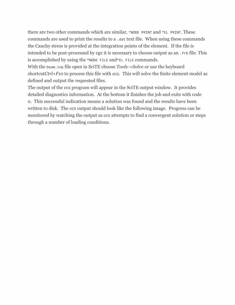
While viewing the colored plot of a results field it is also possible to add the nodal
values. The following images shows top side of the beam’s free end, near x=100, y=0,
z=0. The nodal values are printed in yellow using the commmand plus nv all y. These
values agree with the results of the graph.
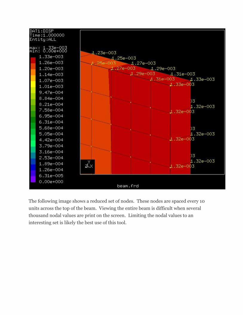
The following image shows a reduced set of nodes. These nodes are spaced every 10
units across the top of the beam. Viewing the entire beam is difficult when several
thousand nodal values are print on the screen. Limiting the nodal values to an
interesting set is likely the best use of this tool.

This concludes the four part tour of Calculix articles. This series is intended not to focus
on the results of a specific problem, but rather to highlight the various functionality
within Calculix and serve as a foundation for future articles. Future articles will delve
into specific functionality and examine the application of Calculix. The functionality
outlined in this series will serve as a common denominator amongst readers. Future
articles will document the specific functionality of a subsystem and rely on this
document to provide the foundation.