Calculation of Converged Rovibrational Energies and...

February 2, 2004

Prepared for publication in J. Chem. Phys.

Calculation of Converged Rovibrational Energies and Partition

Function for Methane using Vibrational-Rotational Configuration

Interaction

Arindam Chakraborty, Donald G. Truhlar

Department of Chemistry and Supercomputing Institute, University of Minnesota,

Minneapolis, MN 55455-0431

Joel M. Bowman, and Stuart Carter

Cherry L. Emerson Center of Scientific Computation and Department of Chemistry,

Emory University, Atlanta, GA 30322

Abstract. The rovibration partition function of CH4 was calculated in the temperature

range of 100–1000 K using well-converged energy levels that were calculated by

vibrational-rotational configuration interaction using the Watson Hamiltonian for total

angular momenta J = 0–50 and the MULTIMODE computer program. The configuration

state functions are products of ground-state occupied and virtual modals obtained using

the vibrational self-consistent field (VSCF) method. The Gilbert and Jordan potential

energy surface was used for the calculations. The resulting partition function was used to

test the harmonic oscillator approximation and the separable-rotation approximation. The

harmonic oscillator, rigid-rotator approximation is in error by a factor of two at 300 K,

but we also propose a separable-rotation approximation that is accurate within 2% from

100 K to 1000 K.

2

I. INTRODUCTION For accurate calculations of molecular energy levels, spectra, and

thermochemistry, it is essential to take account of anharmonicity and the interaction

between rotation and vibration. The coupling between rotation and vibration is due to

Coriolis and centrifugal terms. A review of perturbation methods to account for

anharmonicity and rotation-vibration coupling was given by Nielsen.1 For a highly

symmetric molecule like methane the anharmonicity and rotation-vibration interactions

may be analyzed using group theory.2,3 Jahn used group theory and first order

perturbation theory to treat rotation-vibration interactions in methane in a series of four

papers.4–7 Later, second order and third order perturbation calculations were reported by

Shaffer et. al.8,9 and by Hecht.10,11 More recently Lee et. al.12 and Wang et. al.13 reported

vibrational perturbation theory calculations on methane using an analytical potential

energy surface.

Another approach to the computation of rovibrational levels of molecules is based

on variational theory. The vibrational self-consistent field (VSCF) method14–19 is one

such variational procedure. The VSCF procedure was extended by Carter et. al.20,21 to

study rovibrational states by using the Whitehead-Handy22,23 implementation of the

Watson24 Hamiltonian. However, the VSCF method is not quantitatively accurate. A

more accurate, systematically improvable procedure is vibrational-rotational

configuration interaction21 (VRCI). The convergence of VRCI calculations can be

accelerated by optimizing the basis functions using VSCF.18 A particularly efficient

scheme, called virtual configuration interaction (VCI) is to use a ground-state VSCF

calculation to generate single-mode functions and to use products of these single-mode

functions (called modals) with rotational basis functions as basis functions with linear

coefficients optimized by the variational principle.20,21 These functions are called

configuration state functions (CSFs). In practice, as explained below, we actually used

this procedure only for total angular momentum quantum number equal to 0. For

the CSFs are constructed by taking the products of the

J

00>J =J VCI eigenvectors

with the rotational basis functions. A key advance21 in systematizing of the procedure is

to organize the calculation using a hierarchical representation20,25 of the potential and

limit the number of coupled modes in any included term to two, three, or four. Carter and

3

Bowman26 used VCI with the hierarchical representation to calculate about a hundred

vibrational levels for various isotopologs of CH4 for J = 0 and 9 levels for CH4 for J = 1.

Once the rovibrational energy levels are obtained by the VCI calculations for all

important values of the angular momentum J, they can also be used to compute partition

functions including full rotation-vibration coupling, but – prior to the present paper – this

has not been done. In a J = 0 calculation, Bowman et. al27 showed that inclusion of

anharmonic terms significantly lowers the zero-point energy of methane from its

harmonic oscillator zero-point energy and increases the J = 0 partition function by a

factor of 3.35–1.62 in the temperature range of 200–500 K; they also estimated rotational

effects by using a calculation of the lowest-energy J = 1 states to estimate the rotational

constant for a separable-rotation calculation.27 Manthe et. al28 have also reported a J = 0

partition function for methane that was obtained using a different technique. The

importance of anharmonicity for the vibrational energy of methane has also been shown

in other recent work.29,30 The present paper includes fully converged vibrational states for

J up to 50 in order to calculate a converged rotation-vibration partition function over the

temperature range 100–1000 K. This is the first fully converged rotation-vibration

partition function for any molecule with more than three atoms.

The potential energy surface used for the present calculations is that of Jordan and

Gilbert,31 which is based on older work by Raff32 and Joseph et. al.33 Although this is not

a quantitatively accurate surface for methane, it is realistic enough for our purposes, and

it has been used for recent rate constant calculations on the hydrogen atom27,34–50 and

oxygen atom51,52 abstractions of a hydrogen atom from methane. Our goal is to obtain

accurate rotation-vibration partition functions for a given realistic potential energy

surface in order to assess the magnitude of the rotation-vibration coupling, and the well

studied Jordan-Gilbert potential provides an ideal testing ground for this purpose.

Section II summarizes the theoretical formulation used in the present work, and

Section III is devoted to the degeneracy and symmetry considerations. The eigenvalue

calculations were carried out using a locally modified version of the MULTIMODE

computer program,53 and Section IV provides details of these calculations. Section V

contains details of the partition function calculations. Section VI presents the results and

discussion. The conclusions drawn from the present study are summarized in Sec. VII.

4

II. QUANTUM MECHANICAL THEORY II.A. Application of the VSCF method for J = 0

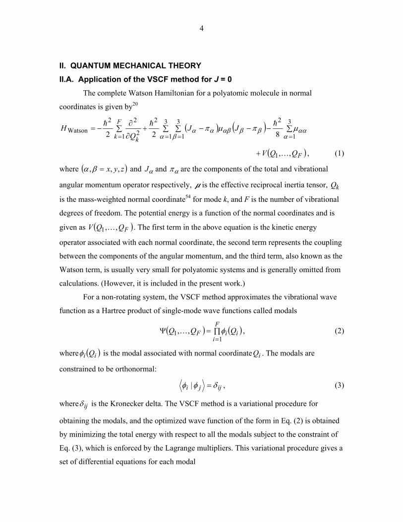
The complete Watson Hamiltonian for a polyatomic molecule in normal

coordinates is given by20

( ) ( ) ∑−∑ ∑ −−+∑∂

∂−=

== ==

3

1

23

1

3

1

2

1 2

22Watson 822 α

ααα β

ββαβαα µπµπ hhh JJQ

HF

k k

( )FQQV ,,1 K+ , (1)

where ( )zyx ,,, =βα and and αJ απ are the components of the total and vibrational

angular momentum operator respectively, m is the effective reciprocal inertia tensor, Qk

is the mass-weighted normal coordinate54 for mode k, and F is the number of vibrational

degrees of freedom. The potential energy is a function of the normal coordinates and is

given as ( )FQQ ,,1 KV . The first term in the above equation is the kinetic energy

operator associated with each normal coordinate, the second term represents the coupling

between the components of the angular momentum, and the third term, also known as the

Watson term, is usually very small for polyatomic systems and is generally omitted from

calculations. (However, it is included in the present work.)

For a non-rotating system, the VSCF method approximates the vibrational wave

function as a Hartree product of single-mode wave functions called modals

, (2) ( ) ∏=Ψ=

F

iiiF QQQ

11 ,, φK ( )

)where ( ii Qφ is the modal associated with normal coordinateQ . The modals are

constrained to be orthonormal:

i

ijji δφφ =| , (3)

where ijδ is the Kronecker delta. The VSCF method is a variational procedure for

obtaining the modals, and the optimized wave function of the form in Eq. (2) is obtained

by minimizing the total energy with respect to all the modals subject to the constraint of

Eq. (3), which is enforced by the Lagrange multipliers. This variational procedure gives a

set of differential equations for each modal

5

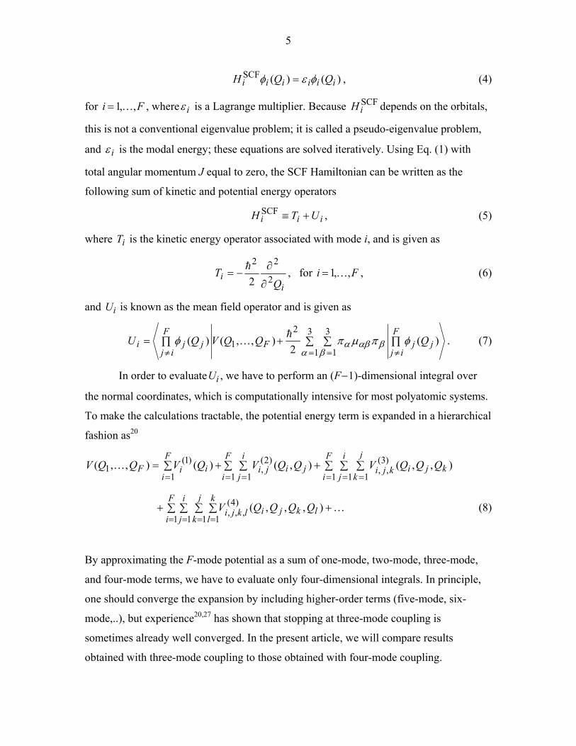
, (4) )()(SCFiiiiii QQH φεφ =

for , wherei =1,K,F iε is a Lagrange multiplier. Because depends on the orbitals,

this is not a conventional eigenvalue problem; it is called a pseudo-eigenvalue problem,

and

SCFiH

iε is the modal energy; these equations are solved iteratively. Using Eq. (1) with

total angular momentum J equal to zero, the SCF Hamiltonian can be written as the

following sum of kinetic and potential energy operators

, (5) iii UTH +≡SCF

where T is the kinetic energy operator associated with mode i, and is given as i

i

iQ

T 2

22

2 ∂

∂−=

h , for i =1,K,F , (6)

and U is known as the mean field operator and is given as i

∏∑ ∑+∏=≠= =≠

F

ijjjF

F

ijjji QQQVQU )(

2),,()(

3

1

3

1

21 φπµπφ

α ββαβα

hK . (7)

In order to evaluateU , we have to perform an (F-1)-dimensional integral over

the normal coordinates, which is computationally intensive for most polyatomic systems.

To make the calculations tractable, the potential energy term is expanded in a hierarchical

fashion as

i

20

∑ ∑ ∑+∑ ∑∑ +== = == ==

F

i

i

j

j

kkjikji

F

i

i

jjiji

F

iiiF QQQVQQVQVQQV

1 1 1

)3(,,

1 1

)2(,

1

)1(1 ),,(),()(),,( K

+ (8) ∑ ∑ ∑ ∑ += = = =

F

i

i

j

j

k

k

llkjilkji QQQQV

1 1 1 1

)4(,,, ),,,( K

By approximating the F-mode potential as a sum of one-mode, two-mode, three-mode,

and four-mode terms, we have to evaluate only four-dimensional integrals. In principle,

one should converge the expansion by including higher-order terms (five-mode, six-

mode,..), but experience20,27 has shown that stopping at three-mode coupling is

sometimes already well converged. In the present article, we will compare results

obtained with three-mode coupling to those obtained with four-mode coupling.

6

The components of the vibrational angular momentum operator depend on two

normal coordinates via the Coriolis coupling constant and are expressed as

πα = −i ζk,lα Qk

∂∂Qll=1

F∑

k=1

F∑ , (9)

where is the Coriolis coupling constant.αζ lk ,55 The treatment of this term and the Watson

term is explained elsewhere.25

II.B. Configuration interaction Since the modes are coupled, one needs to go beyond the VSCF approximation.

The eigenfunctions of the ground-state SCF Hamiltonian for J = 0 form an orthonormal

basis, and the total vibrational wave function can be expanded in this basis; as mentioned

in the introduction, this is called Virtual CI (VCI).20,21 For the calculations in this paper,

we restrict the hierarchical expansion of Eq. (8) to at most four-mode coupling, and we

form the VCI basis by one-mode, two-mode, three-mode, and four-mode excitations from

the ground state. The one-mode excitations are limited by specifying the maximum

number of quanta each mode can possess. Two-mode, three-mode, and four-mode

excitations are limited by two parameters; one of them is the maximum number of quanta

each mode can possess (called maxbas), and the other is the sum of quanta in all the

modes (called maxsum). One could in principle use symmetry to block diagonalize the

Hamiltonian,26 but that was not done for the present calculations.

A general basis function for the VCI calculation is called a configurational state

function (CSF) and is written as Fi nnnn KK21 , where F is the number of modes (9

for methane) and ni is the number of quanta in mode i. All one-mode excitations of the

form Fin 000 21 KK , are included, provided ≤in maxbas(i, 1). All two-mode excited

states of the form Fji nn 000 21 KKK are included, where the sum is less than

or equal to maxsum(2), and n

ji nn +

i and nj are less than or equal to maxbas(i, 2) and maxbas(j,

2), respectively. Similarly, all three-mode and four-mode excitations of the form

Fkji nnn 000 21 KKKK and Flki nnn 000 21 KKKK

kji nnnn

jn K are included, where

is less than or equal to maxsum(3), and kji nnn ++ l+++ is less than or

7

equal to maxsum(4), respectively, and also where ni is less than or equal to maxbas(i, 3)

for three-mode excitations and maxbas(i, 4) for four-mode excitations.21,56

II.C. Application of VCI method to J > 0 For the calculation of rotational-vibrational energy levels, the VCI scheme is applied

with the full Watson Hamiltonian. The rovibrational basis in which the Watson Hamiltonian

is diagonalized is obtained by taking the direct product between the VCI basis functions and

symmetric-top wave functions.20 The symmetric-top wave functions are labeled by three

quantum number MKJ ,, , where J is the angular momentum quantum number, K and M

quantum numbers are associated with the projection of the angular momentum along the

body-fixed z-axis, and the space-fixed Z-axis, respectively

J2 MKJJJMKJ ,,)1(,, 2h+=

MKJKMKJJ z ,,,, h=

MKJMMKJJ Z ,,,, h= . (10)

All exact eigenvalues of the Watson Hamiltonian are independent of M so we consider

only M = 0, and we write 0,, KJ as KJ , . Equation (1) contains terms of the form

where βα JJ zyx ,,, =βα , and the matrix elements of these operators in the KJ , basis

can be obtained using raising and lowering operators. The non-zero matrix elements of all

combinations of angular momentum operators occurring in Watson Hamiltonian have

been given earlier by Bowman et. al.20 and are shown in Appendix A. The matrix

elements are non-zero only for 2,1,0 ±±=∆K

αβ

. In the Watson Hamiltonian, each of these

terms also involve an element µ of the inverse moment of inertia tensor, and the

expressions in Eq. (1) that involve Jx, Jy, Jz also involve the vibrational angular

momentum operators απ . After all the matrix elements of the Hamiltonian are obtained,

the Hamiltonian matrix is diagonalized in this rovibrational basis and the rotation-

vibration energy levels are obtained.

8

III. SYMMETRY AND DEGENERACY OF ROTATION-VIBRATION STATES Symmetry labeling of energy levels gives information about the degeneracies

associated with the energy levels. In the present calculations, methane is treated as a

molecule belonging to the C1 point group. This gives us an opportunity to numerically verify

the degeneracies associated with the vibrational and rovibrational energy levels of methane.

Subsections A and B present a discussion on the symmetry of vibrational and rovibrational

levels that is useful for analyzing the results. The inclusion of nuclear-spin degeneracy

associated with rovibrational levels plays an important role in the computation of the

partition function and is discussed Sec. III.C.

III.A. Vibrational symmetry Methane belongs to the Td point group and has nine vibrational degrees of

freedom, which have only four unique frequencies. Of the nine vibrational modes, there

is one non-degenerate mode with frequency υ1, one doubly degenerate mode with

frequency 2υ , and two triply degenerate modes with frequencies 3υ and 4υ . Note that, in

keeping with the universally accepted language, we sometimes use the word “mode” to

refer to the nine component modes, but elsewhere (as in the rest of this section) it refers

to the four (possibly degenerate) modes. Rather than introducing a new notation when the

above double usage is universally accepted we simply caution the reader about the

context dependence of the word “mode.”

The four modes with unique frequencies 321 ,, υυυ , and 4υ can be labeled using

the irreducible representation of the Td point group, and the symmetry of the vibrational

wave function can be obtained by taking a direct product of these four symmetry labels.

The single degenerate mode with frequency υ1 has symmetry A1, the doubly degenerate

mode with frequency 2υ has E symmetry, and each of the two triply degenerate modes

have symmetry F2. The symmetries of the overtone states of the non-degenerate modes

are obtained by taking a direct product of the symmetries of the fundamental states.

When a mode is degenerate, the symmetries of its overtone states are not obtained simply

by taking a direct product.54 A detailed description on this topic is given elsewhere54

along with a general expression for obtaining the symmetry of overtone states of

9

degenerate modes for any point group. The results of Herzberg57a for the symmetry of

overtone states of degenerate modes of methane are provided in the supporting

information.58 The symmetry of a combination state is obtained by simply taking the

direct product of the individual mode symmetries. For example, a combination state in

which there is one quantum each in 3υ and 4υ will have a symmetry of A1 + E + F1 + F2

and can be obtained by taking a direct product of the F2 irreducible representation with

itself, but an overtone state with two quanta in 3υ and zero quanta in 4υ will span the A1

+ E + F2 irreducible representations.

υ1

Finally, if a combination state arises due to multiple excitation of both degenerate

and non-degenerate modes, the symmetry can be obtained by first evaluating the overtone

symmetries of individual modes using the table in Ref. 57a or from the expression in Ref.

54 and then by taking the direct product of the symmetries associated with the

combination. Note that in the case of methane, evaluating the direct product involving the

symmetry of υ1 is of no consequence since has A1 symmetry.

III.B. Rovibrational symmetry The rotational wave function of any molecule can be labeled by the irreducible

representations of the D group, which is the group of all rotations and reflections. The

irreducible representations are used to represent all rotational states with even J, and

those of are used to represent states with odd values of J. To label the rotational

states of methane one has to reduce the representation of and to the irreducible

representations of the T

i∞

gJD

uJD

gJD

i

uJD

d point group.7 The overall symmetry of the rovibrational wave

function is obtained from the direct product of the symmetries associated with the

vibrational and rotational wave functions in the Td representation. Under the harmonic-

oscillator rigid-rotator approximation, the degeneracy d associated with a generic

rotation-vibration level of methane with n quanta in each i υ and a total angular

momentum of J is given as

d =(n2 +1)(n3 +1)(n3 + 2)(n4 +1)(n4 + 2)(2J +1)2

4. (11)

10

Here we have used the fact that for a harmonic oscillator, a state with n quanta in a

doubly degenerate mode is (n+1)-fold degenerate, and a triply degenerate state with n

quanta of excitation is ((n+1)(n+2)/2)-fold degenerate, and the spherical-top nature of

methane gives the (2J + 1)2 degeneracy associated with the rotational wave function. The

total degeneracy mentioned in Eq. (11) is preserved only for the idealized case of a rigid-

rotator, harmonic oscillator Hamiltonian. The presence of anharmonic effects and

rotation-vibration interactions lift some of the degeneracy. In addition, one must consider

spin, as discussed in Subsection C.

The effect of Coriolis coupling on the vibrational levels of methane has been

studied using group theoretic methods in a series of four papers by Jahn,4–7 and only the

results of those studies that are needed for the present work are summarized here. It was

shown by Jahn that the Coriolis coupling terms in the Watson Hamiltonian transform

according to the F1 irreducible representation of Td point group.6 As a consequence, two

vibrational states will be coupled by Coriolis interaction only when the direct product of

their irreducible representations spans the F1 irreducible representation.6,57b Using the

multiplication table54 for the Td point group, the irreducible representations spanned by

A1 µ A1, E µ E, and F2 µ F2, are given as A1, A1 + A2 + E, and A1 + E + F1 + F2 ,

respectively. Since neither A1 µ A1 nor E µ E spans F1, Coriolis splitting does not occur

for non-degenerate and doubly degenerate modes of methane. It is only the two triply

degenerate modes υ3 and 4υ of F2 symmetry in which the three-fold degeneracy is lifted

due to Coriolis coupling.

The interaction and the symmetry labeling of rovibrational levels of 3υ and 4υ

are best studied using the irreducible representation of the full rotation-reflection group;

hence our first task is to express the symmetry of triply degenerate modes using the

irreducible representations of the full rotation-reflection group. It is shown in Ref. 7 and

in the supporting information58 that is the irreducible representation for J = 1 in the

group, and spans F

u1D

i∞D 2 symmetry in the Td point group. Since the two triply degenerate

modes υ3 and 4υ span F2 symmetry in Td, one finds that υ3 and 4υ span in the

group. To obtain the symmetries of the rovibrational levels, we have to obtain the

u1D

i∞D

11

direct product between and an irreducible representation of a rotational state. One of

the advantages of working in the

u1D

i∞D group is the ease of evaluation of direct products

between two irreducible representations. The direct product between two irreducible

representations of D was discussed by both Wigneri∞

59 and Hamermesh60 and is

summarized by:

×1j

uDJ=

gDJ

u1D

u1

∑=+

−=

21

212

jj

jjJJj DDD . (12)

Using the above equation, the direct product between rotational states and the triply

degenerate vibrational states is given as

, )even(u1

g1

g JDDD JJJ +− ++×

DD −=× . (13) )odd(g1

u1

u JDD JJJ +++

The physical interpretation of this result is that the triply degenerate state has a

vibrational angular momentum associated with it and the vibrational angular momentum

interacts with the total angular momentum through the Coriolis coupling term; the

vibrational angular momentum can be parallel, perpendicular, or antiparallel to the total

angular momentum, which splits the levels. The levels resulting from the splitting of the

triply degenerate state are labeled as F , and , respectively.+F , 0 _F 57b

III.C. Nuclear spin degeneracy The total wave function must be anti-symmetric with respect to exchange of both

the coordinates and spins of identical fermions, and we must take account of this for the

four identical protons in methane. As the Watson Hamiltonian does not include any

nuclear spin, the only effect of inclusion of nuclear spin functions will be to increase the

degeneracy associated with certain rovibrational levels. A system of m identical particles

each with a nuclear spin of I has a total of spin states, and therefore, for

methane the total number of possible spin states is 16. Because the total wave function

must be anti-symmetric with respect to the exchange of any two hydrogen atoms in

methane, not all of the 16-fold degeneracy is allowed for each rovibrational state. In order

mI )12( +

12

to find the correct nuclear spin degeneracy associated with each rovibrational level, one

has to evaluate a direct product between the permutation group symmetries of the

rovibrational and nuclear spin states. The products that are totally symmetric, i.e., that

belongs to the A1 symmetry are the only combinations that exist in nature. The symmetry

of the nuclear spin function for methane is 5A1 + E + 3F2, and Wilson has reported61 a

detailed description of the statistical weights associated with the rovibrational levels.

However, for statistical mechanical calculations at temperatures at which many

rotational levels are occupied, one can replace the individual weights of the rovibrational

state by an average weight to all states.61,62 The average weight is obtained by dividing

the total nuclear spin multiplicity (16 for methane) by the symmetry number (12 for

methane).

IV. EIGENVALUE CALCULATIONS All the calculations were performed using the potential energy surface of Jordan

and Gilbert,31 which was obtained from the POTLIB database.63,64 The rovibrational

energy levels were calculated by the VCI method summarized in Sec. II; these

calculations were carried out using a locally modified version of the MULTIMODE53

program. The zero point energy of the system was taken as the zero of energy for all

tabulated energy levels.

The first step of the calculation involves computation of the J = 0 VSCF

Hamiltonian for the ground-state wave function. In this step the modals are expanded in

harmonic oscillator functions; we used 12 harmonic oscillator functions in each mode. (A

convergence check on this value is presented in Appendix B) The eigenvectors of the

ground-state SCF Hamiltonian were used to perform the VCI calculations and the VCI

matrix was constructed directly from the VSCF modals.

The number of basis functions used for this purpose were controlled by input

parameters. As discussed in Sec. II.B, the VCI basis is formed by using a set of

parameters called maxsum and maxbas. The maximum sum of quanta for one-mode, two-

mode, three-mode, and four-mode coupling was fixed by giving appropriate values to

maxsum(1), maxsum(2), maxsum(3), and maxsum(4). Then the maximum allowed quanta

in mode i for one-mode, two-mode, three-mode, and four-mode excitations was fixed by

13

setting maxbas(i,1), maxbas(i,2), maxbas(i,3), and maxbas(i,4) equal to maxsum(1),

maxsum(1) , maxsum(1) - 2, and maxsum(1) - 3, respectively. As an example, the

procedure for obtaining the VCI basis for J = 0 is as follows. The maximum sum of

quanta was taken to be 7 for one-mode, two-mode, and three-mode excitations, and 6 for

four-mode excitations. The maximum allowed quanta in mode i for one-mode, two-mode,

three-mode, and four-mode excitation was set to 7, 6, 5, and 4, respectively. The resulting

size of the VCI matrix for J = 0 was 5650. In order to study the convergence we also

performed calculations with smaller bases of sizes 715, 868, 1372, 1876, 2065, 2905,

4165, and 4390, and the corresponding maxsum values are shown in Table I.

1−

For , the Hamiltonian matrix was constructed by taking a direct product of

the symmetric-top rotational functions

0>J20 with the eigenfunctions of the J = 0 VCI matrix.

If the NVib lowest-energy eigenfunctions are chosen, the size of the rovibrational matrix

for angular momentum J is given by )12(Vib +JN , and the rovibrational energies are

obtained by diagonalizing a matrix of this order. The values used for NVib are specified

in Sec. VI. Once the rovibrational basis is formed the matrix elements are computed

using the equations in Appendix A. One can also use symmetry of the rovibrational basis

function to expedite the process of forming the matrix, and a detailed description is

presented in Ref. 20. However for the present calculations, methane was treated as a

molecule of C1 symmetry, and this allowed the degeneracies in energy levels associated

with Td point group can be verified numerically.

V. PARTITION FUNCTION CALCULATIONS V.A. Accurate partition function

The canonical partition function was evaluated for a temperature range of 100 K

to 1000 K by summing over all the rovibrational states as

+−∑ ∑∑ +

+=

+

−= TkEKJvEJITQ

J

JK vJ

m

B

G ]),,([exp)12()12()(σ

, (14)

where we have introduced a shorthand for the ground state energy

)0,0,0,,0( 1G ==≡ KJEE FK , (15)

14

and I = 12

, , 4=m σ is the symmetry number, the index v denotes the collection of all

the vibrational quantum numbers, and E(v, J, K) is the M = 0 rovibrational energy that

was obtained by the method discussed in Sec. II (details of the calculations are given in

Sec. IV). The partition function in Eq. (14) can be expressed as

TkEeTQTQ BG

)(~)( −= . (16)

We note for reference that the converged value of E G found in the present work is 9362

cm–1. In the above equation, Q~ has the zero of energy at E G , and Q has the zero of

energy at the minimum valueV of the potential energy. The vibrational partition function

was calculated for the temperature range of 100–1000 K by summing over the computed

vibrational states, and the sum over J in Eq. (14) was carried out through J = 50. The test

for convergence with respect to J was done and the details are provided in the supporting

information.

e

58 The partition functions calculated using the rovibrational levels obtained

by solving the full Watson Hamiltonian were labeled asQ andQ~ without subscripts.

V.B. Approximations to be tested Various sets of approximate partition functions were calculated using the

separable-rotation approximation. Assuming separability of rotational and vibrational

motion, the canonical partition function can be expressed as a product of vibrational

)~( VibQ and rotational ( partition functions )RotQ

RotVibSR~~ QQQ = , (17)

where the subscript “SR” is used to indicate that the partition function is calculated using

the separable-rotation approximation. The vibrational partition function was calculated

using two different methods. In the first method, Vib~Q was calculated from the harmonic

frequencies obtained from normal mode analysis, and this harmonic oscillator vibrational

partition function was labeled as HOVib,~Q . The second method for obtaining Vib

~Q used

the vibrational energies obtained by solving the J = 0 Watson Hamiltonian for the given

potential, and this anharmonic approximation was labeled as 0 Vib,~

=JQ .

15

The rotational partition function together with the nuclear spin contribution for

any nonlinear molecule is given as

∑ −∑ ++

=+

−=

J

JKJ

mTkKJEJI ]),(exp[)12()12(

BRotNuc-Rot σQ , (18)

where J is the angular momentum quantum number, and K is the projection of the angular

momentum along a body-fixed z-axis. If we neglect centrifugal and Coriolis interactions,

the rotational energy of a spherical top depends only on J:

ERot = BJ(J +1) . (19)

In Eq. (19), B is known as the spectroscopic rotational constant. Generally, B is evaluated

from the principal moments of inertia at the equilibrium geometry, and then it is

called . In the present work, the rotational partition function was calculated using two

methods. In the first case was used for calculating the rotational energy by Eq. (19),

and the nuclear-rotational partition function obtained from this method was labeled as

. In the second case, the Watson Hamiltonian was solved for each J value, and

the rotational energies were obtained from the vibrational ground-state energies at each J.

There are vibrational ground state terms corresponding to

eB

Nuc,-

eB

eRotQ

( )12 +J JJK +−= ,,K

50,,1 K=J

Nuc,0-Rot

, and

these were substituted in Eq. (18). The summation was carried out for , and

the computed nuclear-rotational partition function was labeled asQ .

By combining the above treatments, four different separable-rotation partition

functions were obtained and are summarized as follows:

Nuc,0-Rot0 Vib,SR~)GW,(~ QQQ J == , (20)

eNuc,-Rot0 Vib,eSR~)W,(~ QQBQ J ==

Nuc,0-RotHO Vib,SR

, (21)

~)GHO,(~ QQQ = , (22)

eNuc,-RotHO Vib,eSR~)HO,(~ QQB =Q , (23)

where W denotes the use of the Watson Hamiltonian for J = 0, and G denotes the use of the

ground vibrational state for each J.

16

For reference we note that the harmonic approximation to E G

HO,

yields 9530 cm–1 for the

present potential energy surface. Using this value and Eqs. (16) and (20)-(23), we can also

obtain four approximations to Q , namely ( , ( , ( , and . )(T )GW, )W, eB )G )HO,( eB

VI. RESULTS AND DISCUSSION

The zero point energy and the fundamental excitation energies for each of the four

modes are shown in Table II. The average energies and the standard deviation ( of

some excited vibrational levels are shown in Table III. Note that under the harmonic

oscillator approximation, each vibrational state discussed in Table III will be d-fold

degenerate. (From this point on, we are discussing only M = 0 states. The full degeneracy

is always ( times greater due to M degeneracy.) The value of d is

where can be obtained by solving Eq. (11) with J = 0 for each vibrational

level. However, the presence of anharmonic terms couples the normal modes resulting in

partial loss of the d-fold degeneracy. A detailed description of the influence of

anharmonicity on degenerate vibrational states of T

)∆

)12 +J

)1+2(0 Jd 0d

d molecules is given in Ref. 57c. It

should be noted that lifting of the d-fold degeneracy is partial, and some states do not lose

their degeneracy due to anharmonicity. Table III illustrates this for several vibrational

states whose degeneracy is split by anharmonicity. The standard deviation for each

group of states considered in Table III was computed using the following expression

∆

1

)( 2

−

∑ −=∆

d

EEd

ii

, (24)

where Ei is the energy of the state i, and E is the average energy, and d is the

degeneracy in the absence of anharmonicity. Table III also shows the trend in the average

energies and standard deviation with respect to the change in the VCI basis size. It is seen

that increasing the basis has very little effect on the ∆ values. It has been found that the

average energy of states does not decrease monotonically with the VCI basis size. This is

because on increasing the VCI basis size new energy levels are introduced which were

missing in the smaller basis. Incorporation of new states changes the density of states

associated with a given energy level. The density of states associated with the average

17

energies of 5650 VCI basis size is discussed in the supporting information.58 It was also

found that the density of states increases with increasing energy.

As discussed in Sec. III.B, no Coriolis splitting occurs for vibrational states of A1

and E symmetries, and hence these states are expected to be )12( +J and fold

degenerate, respectively, for any J, i.e., d is 1 for A

)12(2 +J

0 1 states and 2 for E states. In Table

IV, the values for the average energy of the vibrational ground state, singly excited

)E(2υ state, and singly-excited )F( 24υ state are listed for a few selected J values along

with their respective standard deviation. The averages and the standard deviation at each

J value for the states were computed over )12( +J , )12(2 +J , and values,

respectively. The A

)12 +J(3

1 and E states showed a much smaller deviation from their respective

mean values as compared to the F2 state, indicating that three-fold degeneracy of the F2

state was removed by Coriolis coupling. Since both A1 and E states are strictly

degenerate states, they should have zero standard deviation, but the results shown in

Table IV have non-zero standard deviation due to the numerical methods used for

computing them. This issue is discussed for the recent paper on H3O+ and D3O+.65

The effect of rotation-vibration coupling was also studied for various J values; the

details of these studies are presented in both Appendix B and supporting information.58

As discussed in Sec III.B, group theoretical methods provide us with the degeneracies

associated with various rovibrational levels, and the numerical results were found to be in

good agreement with the values predicted using group theory. The effect of using a 3-

mode and a 4-mode representation on rovibrational energies was studied using J = 20 as

an example. It was found that by increasing the representation from 3-mode to 4-mode,

the minimum and the maximum rovibrational energies decreased by 2.5 and 5.7 cm-1,

respectively. This change corresponds to about 0.1% and is considered to be very small.

The expression for the partition function can be rewritten as

∑=J

J TQTQ )(~)(~ , (25)

where QJ~ is the contribution from each J level and is defined as

−∑ ∑

++=

+

−= TkKJvEIJTQ

J

JK v

mJ

B

),,(exp)12()12()(~σ

. (26)

18

Since the computational effort to solve for the eigenvalues of the Watson Hamiltonian

with a given increases asJ J2, a compromise was achieved between computational effort

and basis-set optimization effort by dividing the range of angular momentum under study

into subsets and using a different value of for each of them. The size of the

rovibrational matrix is of the order of

VibN

2(Vib )1+JN , and the diagonalization of the

rovibrational matrix becomes computationally expensive for a high value of J and

In order to keep the calculation tractable a converged value of was obtained for the

highest J value for each subset. For example, a converged value of was obtained for

J = 10 and was used for the set of J values in the range 5 < J < 10. A similar procedure

was used for J = 15, 20, and 25, and converged values for Q

.VibN

VibN

NVib

J~ were obtained. A list of

values used at different J states is provided in Table V, and the details of the

convergence studies for these J states are summarized in Table VI, VII, and Appendix C.

The convergence studies were carried out for the temperature range of 100–1000 K and

converged values

VibN

JQ~ were obtained with respect to increasing the size of both the VCI

and the rovibrational basis. For example, Table VI compares the JQ~ values for

obtained from various VCI bases. It is seen that a VCI basis size of 5650 gives converged

values over the entire temperature range. In these calculations, the rovibrational matrix

was formed by using only the lowest functions out of the full 5650 VCI functions.

The value is listed in Table V, and for

10=J

VibN

10VibN =J , was taken to be 500. The size

of the rovibrational matrix formed is of order

VibN

2 )1(Vib +JN , and for a

rovibrational matrix of size 10500

10=J

10500× was diagonalized, and the rovibrational

energies so obtained were used for calculating JQ~ . Convergence with respect to

was checked by forming the rovibrational matrix using half the number of VCI functions.

For , the value of was reduced from 500 to 250 functions and the resulting

size of the rovibrational matrix of

VibN

10=J VibN

52505250× was obtained. As seen from Table VII, a

rovibrational matrix that has only one quarter as many elements leads to a JQ~ value that

differ by less then 0.01% from the one computed with the larger basis. All the energy

19

levels that contributed more than or equal to 10 at 1000 K were include in the

summation in Eq. (26). This corresponds to inclusion in the summation of all states that

are below cm

5−

8000 -1.

)e

Because of the importance of E G for practical calculations, tests of its

convergence are provided in the Appendix B, along with tests of the convergence of

selected individual vibrational energy levels for J = 10–25.

The computed vibrational partition functions are shown in Table VIII. A

converged value of 0=Vib,~

JQ for 1000 K was obtained for a VCI matrix size of 4165.

The vibrational partition function was computed using both 3-mode and 4-mode

representations of the potential energy, and the results are given in Table IX; the 3-mode

representation was found to be sufficiently accurate. In particular the differences of the 3-

mode and the 4-mode results were less that 1%. Convergence with respect to the number

of harmonic oscillator functions was verified, and vibrational partition functions obtained

using 12 and 6 harmonic oscillator functions per modal were found to be within 0.1% of

each other. A similar test was also performed for the Gauss-Hermite integration points,

and the vibrational partition function obtained using 30 and 15 points were within 0.1%

of each other.

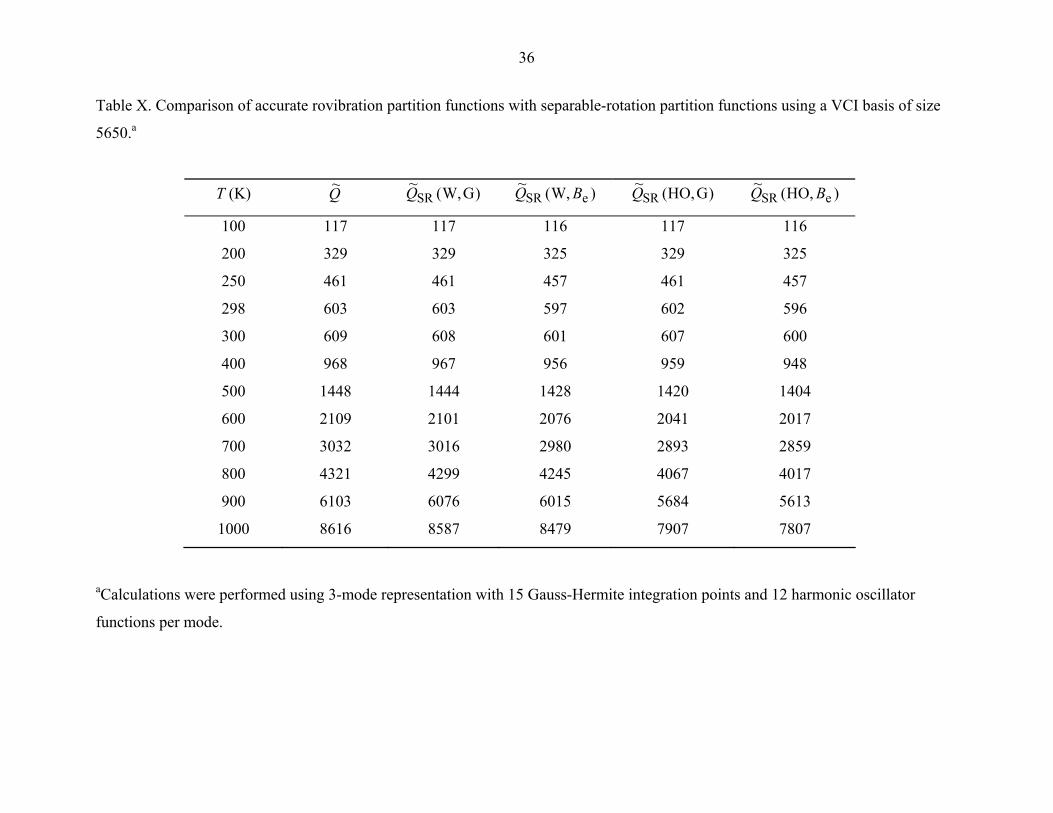
The computed rovibrational partition function and the separable-rotation partition

function are summarized in Table X. It was found that in the low-temperature region, the

rigid-rotator harmonic oscillator HO,(~SR BQ

)~(Q

partition function is very close to the

accurate rovibrational partition function , but the approximation begins to

show significant errors as the temperature is increased, reaching 2% at 400 K and 9% at

1000 K. The separable-rotation partition function

e,HO B

)GW,(~SRQ , as described in Sec. IV,

was found to agree closely with the accurate rotational-vibrational Q~ for all

temperatures; thus this is an inexpensive alternative for computation of accurate

rovibrational partition function. Because the method requires only the vibrational ground

state energies for each of the J > 0 values, it does not require a large VCI and

rovibrational basis.

20

The zero-point inclusive partition function is listed in Table XI, and it was found

that the accurate rovibrational partition function is greater than the rigid-rotator harmonic

oscillator partition function by a factor of 11.4 and 1.4 at 100 K and 1000 K, respectively.

At 300 K the popular harmonic oscillator, rigid-rotator approximation underestimates the

partition function by a factor of 2.3. Although QQ ~ is a more interesting quantity from

the point of view of statistical mechanics (and is the quantity appearing in the textbooks),

is the more interesting quantity from the point of view of practical applications

because errors in calculating the zero point energy are equally as problematic as errors in

calculating the thermal contributions. Again, the W,G approximation performs well. We

should keep in mind, though, that CH

Q

4 is probably close to a “best case scenario” for

separable-rotation approximations in that the lack of any low-frequency modes greatly

decreases the importance of rotation-vibration coupling. Now that we have demonstrated

the feasibility of full thermodynamic rotation-vibration calculations for a pentatomic

molecule, it will be interesting to test approximate theories for molecules with lower

frequencies and large-amplitude motion.

VII. CONCLUSIONS

Fully converged rotational-vibrational partition functions of methane were computed

by summing over the rovibrational levels for the temperature range of 100-1000 K, and the

accurate results were compared with partition functions obtained using the separable-rotation

approximation. The eigenvalues of the full Watson Hamiltonian were obtained using the

computer program MULTIMODE and were converged with respect to VCI basis. The

eigenvalues also showed the expected trends in degeneracy for a given J value. The

difference in vibrational partition function for 3-mode and 4-mode expansion of the potential

was found to be negligible for the present work.

VIII. ACKNOWLEDGMENTS This work was supported in part by the National Science Foundation under grant no.

CHE00-92019, and by the office of Naval Research (ONR-N00014-01-1-0235).

21

APPENDIX A The angular momentum matrix elements needed for the VCI calculations are as

follows:20

JK Jz JK = K (A1)

22 KJKJJK z = (A2)

JKJJKJKJJK yx22 =

])1([21 2KJJ −+= (A3)

JK ±1Jx JK = mi JK ±1Jy JK

21)]1)([(2

+±= KJKJimm (A4)

JKJJKJKJJK yx22 22 ±−=±

21)]1)()(2)(1[(41

−+±+±−= KJKJKJKJ mm (A5)

JKJJJKJKJJJK xyyx −=

)2(iK−= (A6)

JKJJJKiJKJJJK yzxz 1±=1± m

= (K ±1) JK ±1Jx JK (A7)

JKJJJKiJKJJJK zyzx 1±=1± m

JKJJKK x1±= (A8)

JK ± 2 JxJy JK = JK ± 2 JyJx JK

21)]1)()(2)(1[(4

+±+±− KJKJKJKJimmm= (A9)

Notice that we have corrected two typos in Ref. 20.

22

APPENDIX B Table B-I provides the details of the convergence rate of the ground-state energy

E G using different VCI bases. The table also compares the E G values obtained using 3-mode

and 4-mode representations of the potential energy term. The ground-state energy obtained

using different harmonic oscillator functions for each mode is also listed. Comparisons of the

convergence for levels with J > 0 are more cumbersome because of the splitting associated

with the (2J + 1) values of the energy corresponding to different values of K for a given set

of vibrational quantum numbers and a given total angular momentum J; however it is

interesting to compare the convergence of the lowest-energy and highest-energy K state, and

this is done in Table B-II for J = 10. Similar comparison for higher values of J = 15, 20, and

25 is provided in the supporting information.58

Table B-III and B-IV list the rovibrational states associated with the 0001 vibrational

state for J =1 and 20, respectively. The 0001 vibrational state is three-fold degenerate and

belongs to the F2 irreducible representation of the Td point group. (As in main text, we

discuss only M = 0 states; there is an additional degeneracy of a factor ( due to M

states, but this factor is not included in the present discussion.) The number rovibrational

state associated with the 0001 vibrational state for any value of J is given by3 . Using

this relation, the total number of rovibrational states for J = 1 and 20 are 9 and 123,

respectively.

)12 +J

2( )1+J

As discussed in Sec. III.B and Eq. (13), the rovibrational states can be labeled using

the irreducible representations of the i∞D symmetry group. The F2 state of Td point group

transforms according to the irreducible representation of the u1D i

∞D group. The

rovibrational states associated with any J value are given as

23

, (B1) )even(u1

gu1

gu1 JDDDDD JJJJ +− ++=×

. (B2) )odd(g1

ug1

uu1 JDDDDD JJJJ +− ++=×

For J = 1 and 20, the rovibrational states are givens as,

, (B3) g2

u1

g0

u1

u1 DDDDD ++=×

. (B4) u21

g20

u19

g20

u1 DDDDD ++=×

The rovibrational levels associated with each irreducible representation are given by )12( +J

states. For J = 1 case, the , , and representations contribute 1, 3, and 5 states,

respectively. For J = 20, the , , and representations contribute 39, 41, and 43

states, respectively, towards the total of 123 sates. The representations can then be expressed

in terms of the irreducible representation of the T

g0D u

1D

u19D

g2D

g20D u

21D

d point using the following relations61

, (B5) 1g0 A=D

(B6) 2u1 F=D

(B7) 2g2 FE +=D

(B8) 21u19 F10E3A3 ++=D

(B9) 21g20 F10E4A3 ++=D

. (B10) 21u21 F11E3A4 ++=D

The rovibrational levels associated with the 0001 vibrational state with J = 1 are

presented in Table B-III. The rovibrational states are symmetry labeled as A1 + E + 2F2 and

exhibit the degeneracies associated with each symmetry label. For J = 20, the number of

24

states arising from the , , and representations are 39, 41, and 43, respectively,

and are listed in Tables B-IV. It was found that the difference in energies of any two states

belonging to different irreducible representation was very high as compared to the energy

difference between consecutive states belonging to same irreducible representations. Because

of the small energy difference between consecutive states it was not possible to assign T

u19D g

20D

u21D

u21D

d

symmetry labels to each of them, but the appreciable energy difference between the states

belonging to , , and allowed us to divide the 123 rovibrational states in groups

of 39, 41 and 43 states as predicted from the group theoretical treatment. The rovibrational

energies obtained using the 4-mode representations are also shown in Table B-IV, and it was

found that for the given set of rovibrational energies the 3-mode and the 4-mode

representations gave converged results.

u19D g

20D

APPENDIX C This appendix shows convergence studies similar to Table VI and VII (discussed

in Sec. VI) but for J = 15, 20, and 25. These results are in Tables C-I to C-VI.

25

References 1H. H. Nielsen, Rev. Mod. Phys. 23, 90 (1951). 2D. M. Dennison, Rev. Mod. Phys. 3, 280 (1931). 3D. M. Dennison, Rev. Mod. Phys. 12, 175 (1940). 4H. A. Jahn, Proc. Roy. Soc. A 168, 469 (1938). 5H. A. Jahn, Proc. Roy. Soc. A 168, 495 (1938). 6W. H. J. Childs and H. A. Jahn, Proc. Roy. Soc. A 169, 451 (1939). 7H. A. Jahn, Proc. Roy. Soc. A 171, 450 (1939). 8W. H. Shaffer, H. H. Nielsen, and L. H. Thomas, Phys. Rev. 56, 895 (1939). 9W. H. Shaffer, H. H. Nielsen, and L. H. Thomas, Phys. Rev. 56, 1051 (1939). 10K. T. Hecht, J. Mol. Spectry. 5, 355 (1960). 11K. T. Hecht, J. Mol. Spectry. 5, 390 (1960). 12T. J. Lee, J. M. L. Martin, and P. R. Taylor, J. Chem. Phys. 102, 254 (1995). 13X.-G. Wang and E. L. Sibert, Spectrochemica Acta, Part A 58, 863 (2002). 14J. M. Bowman, J. Chem. Phys. 68, 608 (1978). 15G. C. Carney, L. L. Sprandel, and C. W. Kern, Adv. Chem. Phys. 37, 305 (1978). 16T. C. Thompson and D. G. Truhlar, Chem. Phys. Lett. 75, 87 (1980). 17J. M. Bowman, Acc. Chem. Res. 19, 202 (1986). 18R. B. Gerber and M. A. Ratner, Adv. Chem. Phys. 70, 97 (1988). 19D. A. Jelski, R. H. Haley, and J. M. Bowman, J. Comp. Chem. 17, 1645 (1996). 20S. Carter, J. M. Bowman, and N. C. Handy, Theor. Chem. Acc. 100, 191 (1998). 21S. Carter and J. M. Bowman, J. Chem. Phys. 108, 4397 (1998). 22R. J. Whitehead and N. C. Handy, J. Mol. Spectry. 55, 356 (1975).

23R. J. Whitehead and N. C. Handy, J. Mol. Spectry. 59, 459 (1976). 24K. G. Watson, Mol. Phys. 15, 479 (1968). 25S. Carter, S. J. Culik, and J. M. Bowman, J. Chem. Phys. 107, 10458 (1997). 26S. Carter and J. M. Bowman, J. Phys. Chem. A 104, 2355 (2000). 27J. M. Bowman, D. Wang, X. Huang, F. Huarte-Larrañaga, and U. Manthe, J. Chem.

Phys. 114, 9683 (2001). 28U. Manthe and F. Huarte-Larrañaga, Chem. Phys. Lett. 349, 321 (2001). 29D. W. Schwenke, Spectrochemica Acta, Part A 58, 849 (2002).

26

30X.-G. Wang and T. Carrington, Jr., J. Chem. Phys. 118, 6946 (2003). 31M. J. T. Jordan and R. G. Gilbert, J. Chem. Phys. 102, 5669 (1995). 32L. M. Raff, J. Chem. Phys. 60, 2220 (1974). 33T. R. Joseph, R. Steckler, and D. G. Truhlar, J. Chem. Phys. 87, 7036 (1987). 34H.-G. Yu and G. Nyman, J. Chem. Phys. 111, 3508 (1999). 35M. L. Wang, Y. Li, J. Z. H. Zhang, and D. H. Zhang, J. Chem. Phys. 113, 1802 (2000). 36H.-G. Yu, Chem. Phys. Lett. 332, 538 (2000). 37F. Huarte-Larrañaga and U. Manthe, J. Chem. Phys. 113, 5115 (2000). 38F. Huarte-Larrañaga and U. Manthe, J. Phys. Chem. A 105, 2552 (2001). 39D. Wang and J. M. Bowman, J. Chem. Phys. 115, 2055 (2001). 40J. Pu, J. C. Corchado, and D. G. Truhlar, J. Chem. Phys. 115, 6266 (2001). 41G. D. Billing, Chem. Phys. 277, 325 (2002). 42J. Palma, J. Echave, and D. C. Clary, J. Phys. Chem. A 106, 8256 (2002). 43F. Huarte-Larrañaga and U. Manthe, J. Chem. Phys. 116, 2863 (2002). 44M. Wang and J. Z. H. Zhang, J. Chem. Phys. 116, 6497 (2002). 45J. Pu and D. G. Truhlar, J. Chem. Phys. 117, 1479 (2002). 46M. Szichman and R. Baer, J. Chem. Phys. 117, 7614 (2002). 47M. Yang, D. H. Zhang, and S.-Y. Lee, J. Chem. Phys. 117, 9359 (2002). 48D. Wang, J. Chem. Phys. 117, 9806 (2002). 49D. Wang, J. Chem. Phys. 118, 1184 (2003). 50X. Zhang, G.-H Yang, K. L. Han, M. L. Wang, and J. Z. H. Zhang, J. Chem. Phys. 118,

9266 (2003). 51 J. C. Corchado, J. Espinosa-Garcia, O. Roberto-Neto, Y.-Y. Chuang, and D. G.

Truhlar, J. Chem. Phys. A 102, 4899 (1998). 52M.-L. Wang, Y.-M. Li, and J. Z. H. Zhang, J. Phys. Chem. A 105, 2530 (2001). 53S. Carter and J. M. Bowman, MULTIMODE-version 4.6, Department of Chemistry,

Emory University, Atlanta, GA, 2000. 54E. B. Wilson, J. C. Decius, and P. C. Cross, Molecular Vibrations (Dover, New York,

1980), pp. 106-113, pp. 331-332, pp. 352-358.

55D. Papousek and M. R. Aliev, Molecular Vibrational-Rotational Spectra (Elsevier,

New York, 1982).

27

56S. Carter, H. M. Shnider, and J. M. Bowman, J. Chem. Phys. 110, 8417 (1999). 57G. Herzberg, Infrared and Raman Spectra of Polyatomic Molecules (Lancaster Press,

Inc., New York, 1945), (a) pp. 125-127, (b) pp. 446-452, (c) p. 210. 58Supporting information. 59E. P. Wigner, Group Theory and its Application to the Quantum Mechanics of Atomic

Spectra (Academic Press, New York, 1959), p. 187. 60M. Hamermesh, Group Theory and its Application to Physical Problems (Dover, New

York, 1989), p. 369. 61E. B. Wilson, Jr., J. Chem. Phys. 3, 276 (1935). 62J. Kassel, J. Am. Chem. Soc. 55, 1351 (1933). 63R. J. Duchovic, Y. L. Volobuev, G. C. Lynch, D. G. Truhlar, T. C. Allison, A. F.

Wagner, B. C. Garrett, and J. C. Corchado, Comp. Phys. Commun. 144, 169-187

(2002). 64R. J. Duchovic, Y. L. Volobuev, G. C. Lynch, A. W. Jasper, D. G. Truhlar, T. C.

Allison, A. F. Wagner, B. C. Garrett, J. Espinosa-Garcia, and J. C. Corchado,

POTLIB-online, http://comp.chem.umn.edu/potlib. 65X. Huang, S. Carter, and J. M. Bowman, J. Chem. Phys. 118, 5431 (2003).

28

Table I. Values of maxsum used for forming various sizes of VCI basis for J = 0.

maxsum(1,2,3,4) VCI size

4 4 4 4 715

5 5 4 4 868

5 5 5 4 1372

5 5 5 5 1876

6 6 5 5 2065

6 6 6 5 2905

6 6 6 6 4165

7 7 6 6 4390

7 7 7 6 5650

29

Table II. Fundamental excitation energies for J = 0.a,b

υ1υ2υ3υ4 Energy (cm-1)

1000 (A1) 2771

0100 (E) 1444 1444

0010 (F2)

2930 2933 2933

0001 (F2) 1282 1282 1283

aCalculations were performed using 3-mode representation with 15 Gauss-Hermite integration points and 12 harmonic oscillator

functions per mode. bThe zero point energy is 9362 cm-1.

30

Table III. Average energy (in cm-1) and standard deviationa of excited vibrational states for J = 0 with different sizes of VCI basis.b υ1υ2υ3υ4 d c 715 868 1372 1876 2065 2905 4165 4390 5650

0002 6 2595 ≤ 35 2587 ≤ 38 2570 ≤ 39 2558 ≤ 35 2555 ≤ 36 2554 ≤ 37 2553 ≤ 37 2553 ≤ 37 2552 ≤ 38

0101

6 2749 ≤ 7 2748 ≤ 7 2716 ≤ 6 2716 ≤ 6 2716 ≤ 6 2715 ≤ 6 2713 ≤ 6 2713 ≤ 6 2713 ≤ 6

0003 10 3880 ≤ 53 3874 ≤ 57 3865 ≤ 60 3862 ≤ 61 3853 ≤ 65 3836 ≤ 66 3822 ≤ 63 3820 ≤ 65 3816 ≤ 67

0102 12 4025 ≤ 30 4024 ≤ 30 4018 ≤ 32 4013 ≤ 33 4012 ≤ 33 4002 ≤ 35 3984 ≤ 36 3984 ≤ 36 3982 ≤ 37

0202 18 5496 ≤ 20 5490 ≤ 19 5469 ≤ 26 5452 ≤ 29 5451 ≤ 28 5444 ≤ 30 5433 ≤ 31 5435 ≤ 33 5430 ≤ 35

0012 18 5542 ≤ 38 5542 ≤ 43 5533 ≤ 42 5525 ≤ 45 5531 ≤ 40 5513 ≤ 51 5484 ≤ 51 5484 ≤ 52 5490 ≤ 47

0111 18 5694 ≤ 18 5689 ≤ 15 5681 ≤ 16 5675 ≤ 18 5676 ≤ 18 5675 ≤ 19 5643 ≤ 15 5643 ≤ 15 5642 ≤ 17

1111 18 8442 ≤ 26 8446 ≤ 24 8459 ≤ 25 8448 ≤ 19 8453 ≤ 31 8436 ≤ 50 8418 ≤ 33 8426 ≤ 30 8423 ≤ 30 aCalculated using Eq. (24). bCalculations were performed using 3-mode representation with 15 Gauss-Hermite integration points and 12 harmonic oscillator

functions per mode. cThis is the degeneracy that the level would have in the absence of anharmonicity; it is the value used in Eq. (24).

31

Table IV. Average energy (in cm-1) and standard deviationa of vibrational states for selected values of J .b

υ1υ2υ3υ4 0d c 1 5 10 15 20 25 50

0000 1 10 ≤ 0 156 ≤ 0 572 ≤ 0 1248 ≤ 0 2182 ≤ 0 3376 ≤ 1 13183 ≤ 7

0100 2 1455 ≤ 0 1603 ≤ 2 2027 ≤ 7 2713 ≤ 14 3661 ≤ 23 4866 ≤ 39 -

0001 3 1294 ≤ 6 1436 ≤ 21 1844 ≤ 39 2564 ≤ 306 3455 ≤ 229 4721 ≤ 440 -

0002

6 2562 ≤ 36 2702 ≤ 45 3101 ≤ 64 3755 ≤ 91 4681 ≤ 129 5839 ≤ 148 - 0101 6 2723 ≤ 8 2868 ≤ 24 3278 ≤ 42 3948 ≤ 67 4864 ≤ 88 6055 ≤ 127 - 0003 10 3825 ≤ 65 3961 ≤ 72 4353 ≤ 90 4995 ≤ 117 5901 ≤ 154 7052 ≤ 173 - 0102 12 3992 ≤ 37 4134 ≤ 49 4534 ≤ 71 5183 ≤ 95 6108 ≤ 141 7257≤ 125 -

aCalculated using Eq. (24). bCalculations were performed using 3-mode representation with 15 Gauss-Hermite integration points and 12 harmonic oscillator

functions per mode. cThe value used in Eq. (24) is . d 0)12( dJ +

32

Table V. NVib values used in the calculations.a J VibN

1 2000

2

1500

3 1000

4 800

5,…,10 500

11,…,15 300

16,..., 20 200

21,..., 25 200

26,..., 30 200

31,..., 50 100

aFor VCI basis of size 5650.

33

Table VI. Convergence of with respect to change in VCI basis size for J = 10.JQ~ a

VCI size 100 K 200 K 300 K 400 K 500 K 600 K 700 K 800 K 900 K 1000 K

715 0.156 9.57 38.09 78.22 126.32 183.84 254.35 342.45 453.33 592.42

4165

0.157 9.60 38.18 78.39 126.68 184.66 256.15 346.03 459.87 603.54

4390 0.157 9.61 38.18 78.39 126.68 184.67 256.16 346.06 459.93 603.65

5650 0.157 9.61 38.18 78.40 126.70 184.69 256.21 346.11 459.88 603.20


functions per mode.

Table VII. Convergence of with respect to the change in rovibrational basis for J = 10.JQ~ a

VibN 100 K 200 K 300 K 400 K 500 K 600 K 700 K 800 K 900K 1000 K

250 0.157 9.60 38.18 78.39 126.68 184.66 256.15 346.01 459.68 602.85

500 0.157 9.61 38.18 78.40 126.70 184.69 256.21 346.11 459.88 603.20


functions per mode.

34

Table VIII. Comparison of 0Vib,

~=JQ for different size of VCI basis.a


715 1.000 1.000 1.008 1.042 1.113 1.230 1.398 1.624 1.918 2.292

868

1.000 1.000 1.008 1.042 1.113 1.231 1.399 1.636 1.922 2.299

1372 1.000 1.000 1.008 1.042 1.114 1.232 1.402 1.632 1.932 2.316

1876 1.000 1.000 1.008 1.042 1.115 1.233 1.405 1.636 1.940 2.329

2065 1.000 1.000 1.008 1.042 1.115 1.234 1.405 1.637 1.941 2.331

2905 1.000 1.000 1.008 1.042 1.115 1.234 1.405 1.638 1.941 2.336

4165 1.000 1.000 1.008 1.042 1.115 1.234 1.406 1.640 1.947 2.342

4390 1.000 1.000 1.008 1.042 1.115 1.234 1.406 1.640 1.947 2.343

5650 1.000 1.000 1.008 1.042 1.115 1.234 1.406 1.640 1.948 2.345


functions per mode.

35

Table IX. Computed 0Vib,~

=JQ values for 3-mode and 4-mode representation, using a VCI basis size of 5650.

T (K) 3-modea 4-modeb

100 1.000 1.000

200

1.000 1.000

300 1.008 1.008

400 1.042 1.042

500 1.115 1.115

600 1.234 1.234

700 1.406 1.405

800 1.640 1.639

900 1.957 1.945

1000 2.342 2.340

aVibration partition function was calculated using 3-mode representation with 15 Gauss-Hermite integration points and 12 harmonic

oscillator functions per mode. bVibration partition function was calculated using 4-mode representation with 15 Gauss-Hermite integration points and 12 harmonic

oscillator functions per mode.

36

Table X. Comparison of accurate rovibration partition functions with separable-rotation partition functions using a VCI basis of size

5650.a

T (K) Q~ )GW,(~SRQ )W,(~

eSR BQ )GHO,(~SRQ )HO,(~

eSR BQ

100 117 117 116 117 116

200

329 329 325 329 325

250 461 461 457 461 457

298 603 603 597 602 596

300 609 608 601 607 600

400 968 967 956 959 948

500 1448 1444 1428 1420 1404

600 2109 2101 2076 2041 2017

700 3032 3016 2980 2893 2859

800 4321 4299 4245 4067 4017

900 6103 6076 6015 5684 5613

1000 8616 8587 8479 7907 7807


functions per mode.

37

Table XI. Comparison of zero-point-inclusive rovibration partition functions with separable-rotation partition functions using a VCI

basis of size 5650.a

T (K) Q )GW,(SRQ )W,( eSR BQ )GHO,(SRQ )HO,( eSR BQ

100

3.74 µ 10-57 3.74 µ 10-57 3.70 µ 10-57 3.31 µ 10-58 3.28 µ 10-58

200 1.86 µ 10-27 1.86 µ 10-27 1.84 µ 10-27 5.54 µ 10-28 5.47 µ 10-28

250 1.84 µ 10-21 1.84 µ 10-21 1.83 µ 10-21 6.99 µ 10-22 6.93 µ 10-22

298 1.42 µ 10-17 1.42 µ 10-17 1.40 µ 10-17 6.27 µ 10-18 6.20 µ 10-18

300 1.93 µ 10-17 1.93 µ 10-17 1.91 µ 10-17 8.59 µ 10-18 8.49 µ 10-18

400 2.30 µ 10-12 2.30 µ 10-12 2.27 µ 10-12 1.24 µ 10-12 1.23 µ 10-12

500 2.89 µ 10-9 2.89 µ 10-9 2.85 µ 10-9 1.75 µ 10-9 1.73 µ 10-9

600 3.76 µ 10-7 3.74 µ 10-7 3.70 µ 10-7 2.43 µ 10-7 2.40 µ 10-7

700 1.33 µ 10-5 1.33 µ 10-5 1.31 µ 10-5 9.00 µ 10-6 8.90 µ 10-6

800 2.11 µ 10-4 2.10 µ 10-4 2.07 µ 10-4 1.46 µ 10-4 1.45 µ 10-4

900 1.93 µ 10-3 1.92 µ 10-3 1.90 µ 10-3 1.37 µ 10-3 1.36 µ 10-3

1000 1.22 µ 10-2 1.21 µ 10-2 1.20 µ 10-2 8.77 µ 10-3 8.66 µ 10-3


functions per mode.

38

Table B-I. Convergence of ground-state energy (in cm-1) with respect to size of VCI basis and number of modes coupled.

VCI size Modes coupled HO function per modal E G 715 3 12 9362.0013

868

3 12 9361.9295

1372 3 12 9361.8600

1876 3 12 9361.8506

2065 3 12 9361.7935

2905 3 12 9361.6712

4165 3 12 9361.5884

4390 3 12 9361.5833

5650 3 12 9361.5661

5650 4 12 9361.5652

5650 3 6 9361.5670

39

Table B-II. Comparison of the minimum and maximum rovibrational energy (in cm-1) of selected vibrational states, computed using

various VCI bases at J = 10.a

K c 715 4165 4390 5650υ1υ2υ3υ4 0d b

min max

min max min max min max min max

0000 1 -4 10 572 573 572 572 572 572 572 572

0100

2 -4 -3 2019 2037 2017 2035 2017 2035 2017 2035

0001 3 8 -1 1795 1898 1792 1894 1792 1894 1792 1894

0002 6 8 -5 3056 3264 3010 3221 3010 3221 3010 3221

0101 6 8 9 3259 3391 3222 3352 3222 3352 3222 3352

0003 10 8 9 4294 4598 4235 4551 4232 4550 4226 4548

0102 12 10 9 4477 4787 4435 4686 4435 4728 4433 4727


functions per mode. bThe minimum and maximum energy levels were selected from 21 states (with M = 0) that have the indicated values of the four

vibrational quantum numbers.

0d

cValues correspond to the VCI basis size of 5650.

40


functions per mode.

Table B-III Rovibrational energies of 0001 vibrational state at J = 1.a

υ1υ2υ3υ4 Energy (cm-1)

0001 (A1) 1283.2

0001 (F2)

1287.8 1287.9 1288.0

0001 (F2) 1296.9 1297.0 1297.1

0001 (E) 1297.3 1297.5

41

Table B-IV Rovibrational energies (in cm-1) of 0001 vibrational state at J = 20 for different

irreducible representationsa with 3-mode and 4-mode coupling.b

39 states u19D 41 states g

20D 43 states u21D

3-mode 4-mode 3-mode 4-mode 3-mode 4-mode

3334.7 3332.1 3395.4 3394.4 3474.5 3474.4

3334.7 3332.1 3395.4 3394.4 3474.6 3474.7

3335.5 3332.2 3395.5 3394.9 3475.5 3474.8

3335.5 3332.2 3395.5 3394.9 3475.5 3475.0

3335.6 3332.4 3395.6 3395.0 3475.6 3475.1

3335.6 3332.4 3395.6 3395.0 3475.9 3475.3

3335.8 3332.5 3410.8 3409.2 3476.1 3475.4

3335.8 3332.5 3410.8 3409.2 3476.4 3475.7

3336.1 3333.3 3411.0 3409.8 3493.1 3490.8

3336.1 3333.3 3411.1 3409.8 3493.2 3490.8

3336.6 3333.4 3411.2 3409.8 3493.3 3490.9

3336.6 3333.4 3411.2 3409.8 3493.9 3491.6

3336.7 3333.7 3422.4 3420.4 3494.3 3491.7

3336.9 3334.0 3422.4 3420.4 3496.2 3493.7

3337.1 3334.0 3422.9 3421.1 3496.3 3493.7

3337.4 3334.3 3422.9 3421.1 3496.4 3493.8

3337.4 3334.5 3423.0 3421.1 3499.1 3496.6

3337.5 3334.5 3423.0 3421.1 3499.4 3496.6

3337.6 3334.5 3431.8 3429.4 3499.5 3496.7

3338.0 3335.0 3431.8 3429.4 3503.9 3501.0

3338.1 3335.1 3432.4 3430.1 3504.1 3501.2

3338.9 3335.9 3432.5 3430.2 3504.2 3501.4

3338.9 3335.9 3432.7 3430.3 3504.3 3501.5

3339.1 3335.9 3432.7 3430.3 3504.8 3501.6

3339.1 3335.9 3438.8 3435.9 3505.1 3502.1

42

bCalculations were performed using 15 Gauss-Hermite integration points and 12 harmonic

oscillator functions per mode.

aThe irreducible representations associated with J = 20 are , , and , and were

obtained using Eq. (B4).

3339.6 3336.6 3439.3 3436.5 3512.5 3509.1

3339.6 3336.6 3440.0 3437.3 3512.5 3509.1

3341.4 3338.3 3440.2 3437.3 3512.7 3509.3

3341.4 3338.3 3440.5 3437.7 3512.7 3509.3

3341.6 3338.4 3440.6 3437.8 3513.2 3509.4

3341.6 3338.4 3444.0 3440.8 3513.2 3509.4

3342.0 3339.0 3444.1 3440.9 3523.0 3518.8

3342.0 3339.0 3444.6 3441.3 3523.0 3518.8

3345.5 3342.2 3448.1 3445.2 3523.2 3519.1

3345.5 3342.2 3448.2 3445.3 3523.2 3519.1

3345.7 3342.3 3448.2 3445.3 3523.7 3519.2

3345.7 3342.3 3449.4 3446.3 3523.7 3519.2

3345.9 3342.9 3450.1 3446.9 3535.9 3530.8

3345.9 3342.9 3450.5 3447.3 3535.9 3530.8

3450.7 3447.3 3536.0 3531.0

3450.9 3447.4 3536.0 3531.0

3536.7 3531.1

3536.7 3531.1

u19D g

20D u21D

43

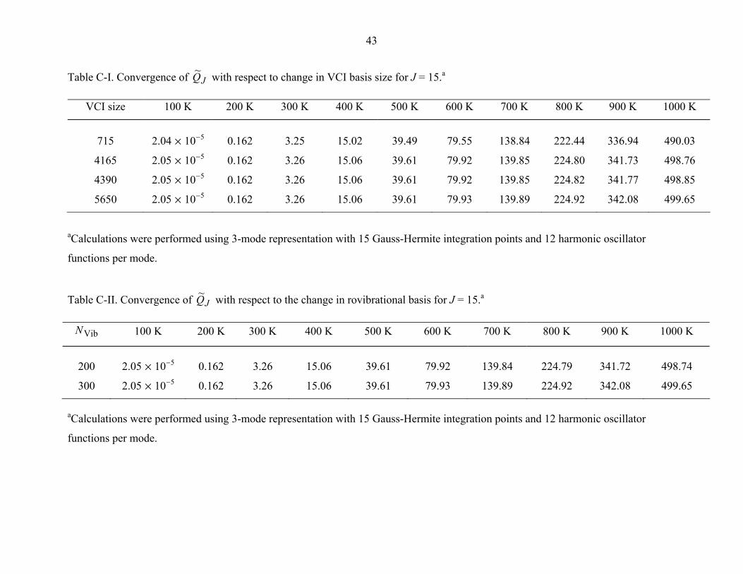
Table C-I. Convergence of with respect to change in VCI basis size for J = 15.JQ~ a


715

2.04 µ 10-5 0.162 3.25 15.02 39.49 79.55 138.84 222.44 336.94 490.03

4165 2.05 µ 10-5 0.162 3.26 15.06 39.61 79.92 139.85 224.80 341.73 498.76

4390 2.05 µ 10-5 0.162 3.26 15.06 39.61 79.92 139.85 224.82 341.77 498.85

5650 2.05 µ 10-5 0.162 3.26 15.06 39.61 79.93 139.89 224.92 342.08 499.65


functions per mode.

Table C-II. Convergence of with respect to the change in rovibrational basis for J = 15.JQ~ a

VibN 100 K 200 K 300 K 400 K 500 K 600 K 700 K 800 K 900 K 1000 K

200

2.05 µ 10-5 0.162 3.26 15.06 39.61 79.92 139.84 224.79 341.72 498.74

300 2.05 µ 10-5 0.162 3.26 15.06 39.61 79.93 139.89 224.92 342.08 499.65


functions per mode.

44

Table C-III. Convergence of with respect to change in VCI basis size for J = 20.JQ~ a


715

5.32 µ 10-11 3.40 µ 10-4 6.43 µ 10-2 0.912 4.70 14.84 35.68 72.56 131.87 220.89

4165 5.17 µ 10-11 3.41 µ 10-4 6.45 µ 10-2 0.915 4.72 14.93 36.01 73.53 134.25 226.00

4390 5.17 µ 10-11 3.41 µ 10-4 6.45 µ 10-2 0.915 4.72 14.93 36.02 73.53 134.26 226.03

5650 5.18 µ 10-11 3.41 µ 10-4 6.45 µ 10-2 0.915 4.72 14.94 36.02 73.56 134.32 226.16


functions per mode.

Table C-IV. Convergence of with respect to the change in rovibrational basis for J = 20.JQ~ a

VibN 100 K 200 K 300 K 400 K 500 K 600 K 700 K 800 K 900 K 1000 K

100

5.18 µ 10-11 3.41 µ 10-4 6.45 µ 10-2 0.915 4.72 14.93 36.01 73.53 134.25 226.00

200 5.18 µ 10-11 3.41 µ 10-4 6.45 µ 10-2 0.915 4.72 14.94 36.02 73.56 134.32 226.16


functions per mode.

45

Table C-V. Convergence of with respect to change in VCI basis size for J = 25 JQ~

______________________________________________________________________________________________________________________________________________________________


______________________________________________________________________________________________________________________________________________________________

715 2.78 µ 10-18 9.83 µ 10-8 3.26 µ 10-4 1.93 µ 10-2 0.236 1.330 4.77 13.12 29.99 59.99

4165 2.80 µ 10-18 9.87 µ 10-8 3.27 µ 10-4 1.94 µ 10-2 0.237 1.329 4.82 13.34 30.69 61.83

4390 2.80 µ 10-18 9.87 µ 10-8 3.27 µ 10-4 1.94 µ 10-2 0.237 1.329 4.82 13.34 30.69 61.84

5650 2.80 µ 10-18 9.87 µ 10-8 3.27 µ 10-4 1.94 µ 10-2 0.237 1.330 4.83 13.34 30.70 61.86

______________________________________________________________________________________________________________________________________________________________


functions per mode.

Table C-VI. Convergence of with respect to the change in rovibrational basis for J = 25 JQ~

VibN

100 K 200 K 300 K 400 K 500 K 600 K 700 K 800 K 900 K 1000 K

100

2.80 µ 10-18 9.86 µ 10-8 3.26 µ 10-4 1.94 µ 10-2 0.236 1.33 4.83 13.34 30.70 61.86

200 2.80 µ 10-18 9.87 µ 10-8 3.27 µ 10-4 1.94 µ 10-2 0.237 1.33 4.83 13.34 30.70 61.86


functions per mode.

Calculation of Converged Rovibrational Energies and...

Documents

Transcript of Calculation of Converged Rovibrational Energies and...