Calculation of Binding Free Energies - Max Planck Society · PDF filefree energies are among...

173

Andreas Kukol (ed.), Molecular Modeling of Proteins, Methods in Molecular Biology, vol. 1215,DOI 10.1007/978-1-4939-1465-4_9, © Springer Science+Business Media New York 2015

Chapter 9

Calculation of Binding Free Energies

Vytautas Gapsys, Servaas Michielssens, Jan Henning Peters, Bert L. de Groot, and Hadas Leonov

Abstract

Molecular dynamics simulations enable access to free energy differences governing the driving force underlying all biological processes. In the current chapter we describe alchemical methods allowing the calculation of relative free energy differences. We concentrate on the binding free energies that can be obtained using non-equilibrium approaches based on the Crooks Fluctuation Theorem. Together with the theoretical background, the chapter covers practical aspects of hybrid topology generation, simulation setup, and free energy estimation. An important aspect of the validation of a simulation setup is illustrated by means of calcu-lating free energy differences along a full thermodynamic cycle. We provide a number of examples, including protein–ligand and protein–protein binding as well as ligand solvation free energy calculations.

Key words Free energy, Molecular dynamics, Alchemical transitions, Protein–ligand binding, Protein–protein interaction, Non-equilibrium methods, Hybrid topology, Crooks Fluctuation Theorem

1 Introduction

Whether or not a process happens spontaneously is determined by its free energy. This is because, without an external source of energy, systems evolve to their lowest free energy state. Likewise, the rate at which that state is reached depends on free energy barriers along the pathways to that minimum. Hence, free energies are of central importance as they determine, e.g., binding affini-ties (spontaneous binding or not) or protein folding (the folded state is usually the free energy minimum). In addition, as barriers are linked to rates via rate theory, free energy barriers determine binding, folding, permeation, and reaction kinetics. Therefore, free energies are among the most critical thermodynamic quantities to accurately be derived by computational techniques, not only because they play such a fundamental role, but also because they can be directly and quantitatively compared to experimental data.

174

Thermodynamically, a distinction is made between the so- called Helmholtz and Gibbs free energies. The Helmholtz free energy is defined as:

F = -U TS (1)

with U the internal energy, T the temperature, and S the entropy of the system. The Gibbs free energy is defined as:

G TS= -H (2)

with H the enthalpy of the system, defined as H = U + pV, with p the pressure and V the volume of the system.

Importantly, note that both definitions contain a term that is dependent on the internal (or potential) energy of the system, and another that depends on the entropy. This has the important impli-cation that free energies, and hence, affinities or stabilities, are affected by both changes in interatomic interactions as well as entropic changes. Particularly, changes in solvent entropy can play a substantial or even dominant role as, e.g., in the hydrophobic effect, where solvent molecules are set free upon the formation of a hydrophobic protein or membrane core.

The difference between the Helmholtz and Gibbs free energy lies in the pV term. The Helmholtz free energy is applicable at constant volume, whereas the Gibbs free energy is used at constant pressure, where the pV term quantifies the work associated with a change in volume. Under physiological conditions and for a typical experimental setup we usually have isobaric conditions, hence the Gibbs free energy gradient acts as a driving force for a system. While we will return to the concepts of the Helmholtz and Gibbs free energies in Subheading 2.1, for the practical examples in this chapter we will focus on the Gibbs free energy.

In addition to being the quantity that is minimized at equilib-rium, the free energy is also the maximum amount of energy that can be obtained from a spontaneous process at constant tempera-ture, or conversely, the minimum amount of energy required to drive an uphill process. More precisely, the free energy is the energy obtained from (or required to drive) a process slow enough such that it is in equilibrium with its surroundings at all times. If enforced faster, friction results in non-equilibrium work values that on aver-age are larger than the associated free energy change. The excess energy is dissipated as heat. Traditional free energy methods there-fore require transitions slow enough such that the systems under investigation can be considered to be in equilibrium at all times. Remarkably, however, with the Jarzynski equality and the Crooks Fluctuation Theorem (CFT) given, free energies can also be derived from non-equilibrium work distributions, as described further below.

Vytautas Gapsys et al.

175

An important implication of the free energy follows from its role in statistical mechanics, stating that the probability to be in state x is directly related to its free energy:

p x e G x k TB( ) ( )µ - /

(3)

where kB is the Boltzmann constant. The term e G x k TB- ( )/ is called the Boltzmann factor. This relation is particularly useful to estimate free energy differences between two states A and B:

p Ap B

e eG A G B k T G k TB B( )( )

( ( ) ( ))= =- - -/ D /

(4)

which also presents the most straightforward way to estimate free energies from simulation: provided that a sufficiently converged ensemble is available, usually requiring several reversible transitions between A and B, the free energy difference ΔG can directly be esti-mated from this relation by evaluating the populations in A and B.

Alternative simulation approaches to derive free energies are frequently tailored towards overcoming or avoiding free energy barriers associated, e.g., with binding, unbinding, conformational transitions, or (re)folding. Examples include, umbrella sampling [1] and thermodynamic integration [2]. In umbrella sampling, a biasing potential is employed to enforce transitions across high energy states along a predefined reaction coordinate. The effect of the biasing potential can be corrected for afterwards, yielding the free energy profile for a one-dimensional reaction coordinate or the free energy landscape for a multi-dimensional reaction coor-dinate. In thermodynamic integration and other alchemical appro-aches, the sampling of cumbersome binding and unbinding events is prevented by instead carrying out a transition in chemical space where the Hamiltonian describing system A is transformed into B. Making use of the fact that the free energy is a state variable, the relative free energy change can be estimated from the difference of the associated transition free energy for example in the context of a protein binding pocket and the same transformation in solution, for the calculation of relative binding free energies.

A remarkable characteristic of the free energy is that in many cases, its estimate converges faster than either the individual enthalpy and entropy contributions. This is due to the fact that the largest contributions to both arise from a solvent–solvent term that occurs in both but that exactly cancels out in the free energy estimate [3].

This chapter mainly focuses on the use of non-equilibrium methods for the calculation of binding free energies. For equilib-rium approaches, we refer to excellent reviews in the literature [4–6].


176

2 Theory

The free energy surface of a system completely describes its thermodynamic and kinetic properties. An intuitive interpretation of the free energy is provided by its relation to the probability pA of finding the system in a phase space volume A:

p

eeA

F

F

A

=-

-

b

b

(5)

where FA is the free energy of a phase space volume A, F is the Helmholtz free energy evaluated over the whole phase space, and β = 1∕kBT, with the Boltzmann constant kB and temperature T. In most practical cases the differences between the state popula-tions are of interest in contrast to the absolute free energy values. By considering two states, A and B, the free energy difference ΔFAB can be expressed as

DF F F

p QQAB B A

B

A

B

A

= - = - = -1 1b

ln lnp b

(6)

Q denotes the canonical partition function: Q = Q (N, V, T ), with N number of particles and V volume of a container. The free energy is related to the partition function via F = −1 ∕ β ln Q (N, V, T ).

From the latter expression (Eq. 6) several approaches to obtain-ing ΔF can be deduced. Firstly, a direct counting of events sam-pling phase space volumes A and B immediately enables access to the probabilities pA and pB. For example, in case of molecular bind-ing, this method could be employed by simulating two molecules of interest (ligands A and B) and directly counting their respective probabilities of being in bound/unbound forms. While the approach is simple, its computational cost for large biologically relevant systems is usually beyond reach for the current state-of-the-art atomistic simulations.

Another method requires evaluation of the partition functions. However, while for an ideal gas example, the partition function has an analytical expression, for particles with complex interactions a numerical integration over the coordinates and momenta is required. A canonical partition function is defined as follows:

Q N V T

h Ne d d d dN

HN N

N N( , , )!

( , )= ¼ ¼ ¼- ¼ ¼13 1 1

1 1ò ò b p p q q p p q q

(7)

where H(p, q) is a Hamiltonian of a system, q and p denote coor-dinates and momenta, respectively, h is Planck’s constant. For a multi-particle system, integration over all the degrees of freedom is not computationally feasible. Hence, a simulation is often used to sample the accessible phase space volume. In a simulation, high

2.1 Definition of Free Energy


177

energy microstates will be visited only rarely (or will not be visited at all), hence, rendering this approach unsuitable for the estimation of absolute free energies. For the free energy differences, however, the inaccessible phase space regions will be discarded for both states, A and B, thus allowing for an accurate assessment of ΔF due to cancellation of errors.

Up to now, we considered a canonical ensemble with the asso-ciated canonical partition function Q and Helmholtz free energy F. In practice, however, experimental measurements are usually performed at isothermal-isobaric conditions generating an NPT ensemble. In such a case, a partition function is defined as

Q N P T

h Ne dVd d d dN

H PVN N

N N( , , )!

( ( , ) )= ¼ ¼ ¼- ¼ ¼ +13 1 1

1 1ò ò b p p q q p p q q

(8)

where P is the pressure. The Gibbs free energy is defined as G = −1 ∕ β lnQ (N, P, T ). For the remainder of this chapter we assume constant pressure and therefore focus on the NPT ensem-ble with the associated Gibbs free energy. By considering the fact that a Hamiltonian of a system consists of a kinetic and potential energy components H(p, q) = K(p) + U(q), the partition function can be separated into kinetic and configurational partition func-tions. As the K(p) component depends only on the particle momenta, the kinetic partition function for states A and B does not change as long as there is no perturbation of mass between the states. Therefore, for the sake of simplicity, often only the configu-rational partition function is used. However, in this chapter, we will use a more general approach by considering the full Hamiltonian of a system.

In the following section, we will briefly introduce the most popular approaches for free energy estimation from equilibrium simulations. Further, we will concentrate on the conceptually dif-ferent approaches relying on non-equilibrium transitions between states.

The free energy perturbation (FEP) method introduced by Zwanzig [7] (Pohorille et al. [8] attribute the first derivation to Landau [9]) can be derived from Eq. 6:

DG G G

QQ

eAB B AB

A

H H

AB A= - = - = - - -1 1

b bbln ln ( ( , ) ( , ))p q p q

(9)

where the angular brackets ¼ denote an ensemble average. The approach relies on equilibrium sampling at state A and subsequent evaluation of the produced configurations with the Hamiltonian of state B. The Hamiltonian is controlled by an external parameter often denoted as λ: H Hl l( , ) ( , , )p q p q= . The accuracy of the FEP method is strongly dependent on the phase space overlap of the states A and B. In case the overlap is small, the configurations

2.2 Free Energy Estimates from Equilibrium Simulations: Perturbation Method


178

generated at state A will be identified as high energy microstates when evaluated with the Hamiltonian HB(p, q), in turn contributing little to the exponential average. Hence, the approach is known to converge slowly and is only tractable for the ΔG estimation between the states exhibiting large overlap in the phase space. More informa-tion concerning the accuracy, convergence, and usage of FEP can be found in [8, 10–12].

Another method to estimate ΔG from end state equilibrium sampling was proposed by Bennet and is referred to as Bennet’s Acceptance Ratio (BAR) [13]. Bennet’s estimate is expressed by:

DG

f H H C

f H H CCAB

A B B

B A A

=- +

- -+

1b

ln( ( , ) ( , ) )

( ( , ) ( , ) )

p q p qp q p q

(10)

here f represents Fermi function f(x) = 1∕(1 + exp(βx)) and

CQQ

nn

A

B

B

A

=æ

èç

ö

ø÷

1b

ln , nA and nB are the numbers of configurations

generated in the states A and B, respectively. Equation (10) can be solved numerically by finding such C, that

å å- + = - -

BA B

AB Af H H C f H H C( ( , ) ( , ) ) ( ( , ) ( , ) )p q p q p q p q

(11)

Having determined C yields the free energy difference:

DGnn

CB

A

= - +1b

ln . BAR is a minimal variance free energy estimate.

Shirts et al. [14] also derived Bennet’s formula using maximum likelihood formulation, thus, demonstrating that BAR provides the most likely free energy estimate for the observed work distributions.

Both methods introduced so far (FEP and BAR) were defined for free energy calculations by sampling physical end states of a system. Simulations, however, allow accessing unphysical (alchemi-cal) pathways as well, by coupling the Hamiltonians of the two states H H HA Bl l l= - +( )1 . Different λ dependent coupling functions have been investigated [15, 16]. For the λ values 0 and 1, the system is at the physical states A and B, respectively, whereas for the values 0 < λ < 1 the system is in a mixed unphysical state. The path between the states A and B can be divided into discrete states (also called stratification). Performing equilibrium simulations at the intermediate states ensures a larger phase space overlap between the ensembles adjacent to one another along the λ coordinate. FEP or BAR estimators can be employed to obtain free energy differ-ences between the intermediate states which can later be summed up to yield ΔGAB between the physical end states. The weighted histogram analysis (WHAM) [17] and multistate Bennet Acceptance Ratio (MBAR) [18] methods were developed to estimate free


179

energy difference by considering all intermediate states simultaneously. Ways to achieve an optimal distribution of the discrete states to ensure maximal phase space overlap along the path have also been investigated [19, 20].

A conceptually different method from the ones described above, termed thermodynamic integration (TI) [2], obtains the free energy difference by integrating the average force exerted on the system along the λ variable during an alchemical transition:

D l

l

GH

dAB =¶¶ò

0

1

l (12)

Several approaches have been developed to use thermodynamic integration in simulations. The slow growth TI requires perform-ing transition between the states very slowly, such that the system remains close to equilibrium at all times. In this case, the free energy value is equal to the work done during the transition. Another assumption states that an instantaneous ¶ lH / ¶ value at any λi is equal to an ensemble average at that λi. In practice, due to limited sampling the system is kept at a quasi-equilibrium state, which in turn results in inaccurate free energy estimates as some work is dis-sipated. Convergence issues related to the slow growth TI are well known and have been thoroughly investigated [21–23].

A discrete thermodynamic integration method (DTI) is based on dividing the path along the λ coordinate into discrete steps, similarly as for the FEP and BAR approaches discussed in the previ-ous section. An equilibrium simulation is started at every λi state

and an average ¶¶H

il l

is evaluated. A numerical integration of

the averages directly yields a ΔG value. The accuracy of DTI

depends on the sampling time and distribution of the discrete states. As it was the case for the multi-state FEP and BAR methods, DTI requires phase space overlap between the neighboring ensem-bles along the λ coordinate. The numerical integration scheme was also demonstrated to influence accuracy of the free energy esti-mates [20, 24, 25].

The methods described in the current section rely on the work measurements over non-equilibrium transitions, and hence are sometimes termed NEW. In 1997 Jarzynski derived an identity relating an exponential average of work during non-equilibrium transitions to the free energy difference of the canonical ensemble [26] (it was later shown by Cuendet [27], that the equality also holds for an NPT ensemble):

e eG WAB- -=b bD (13)

2.3 Free Energy Estimates from Equilibrium Simulations: Thermodynamic Integration

2.4 Theory of Non- equilibrium Free Energy Calculations


180

The Jarzynski equality requires the transitions to be started from an equilibrium ensemble. The work values can be obtained from a relation similar to that of thermodynamic integration:

W

Hd=

¶¶ò 0

1

ll

(14)

In contrast to TI, in Eq. 14 instantaneous ¶ ¶H / l values are integrated. The resulting work contains both a contribution from the free energy difference and the dissipated work along the transi-tion path. The FEP approach (Eq. 9) can be viewed as a special case of the Jarzynski equality, where a transition from A to B is per-formed instantaneously.

Similarly to FEP, of which the convergence strongly depends on the phase space overlap between the end states, the accuracy of the free energy differences calculated using Jarzynski’s formula depends on rare events, where little work is dissipated. Fast transi-tions, driving a system far from equilibrium, would yield large work values, contributing little to the exponential average, hence slow-ing the convergence of the ΔG estimation.

Several free energy estimators have been developed based on the Jarzynski equality. In case the transitions are performed in the near equilibrium regime, a Gaussian approximation for the work distribution P(W) is valid due to the central limit theorem [28]. Cumulant expansion of a Gaussian distribution allows expressing the free energy difference as

DG W

n

W= -b s 2

2 (15)

where Wn

is the mean and s W2 is the variance of a P(W) dis tri-

bution. The variance of a free energy estimate is given by s b s

W Wn n2 2 4 2 2/ /+ -( ) , with n denoting number of measured work values. The estimator ought to be used only if the assump-tions for the Gaussian approximation of a work value distribution are fulfilled, i.e. many work values are obtained and the transitions keep the system near equilibrium [29]. Otherwise, the free energy difference can be estimated from the Jarzynski equality directly. Such an estimator, however, has been shown to be biased given a limited number of observed work values [29]. The Jarzynski esti-mator is defined as

D ˆ lnG = - -1

bbe W

n

(16)

A more general relation, enabling the combination of the work value distributions from forward and backward transitions to obtain the Helmholtz free energy difference was derived by Crooks [30, 31].


181

The relation is also known as the Crooks Fluctuation Theorem (CFT). Chelli demonstrated the validity of the Crooks equation for an NPT ensemble [32].

P W

P Wef

r

W G( )

( )( )

-= -b D

(17)

where Pf (W) and Pr(−W) correspond to the work distributions during forward and reverse processes, respectively. The Jarzynski identity can be derived from the Crooks equality, as demonstrated by Crooks [30]. CFT requires that the transitions between the states were started from equilibrium ensembles. However, similar to the Jarzynski identity, there is no requirement for a system to reach an equilibrium at the final state of a transition. A number of estimators have been developed to extract the free energy difference from the work distributions using Crooks equality [14, 33–35].

For the cases where an overlap between the work distributions is large, the free energy difference can be estimated directly from the CFT:

ln

( )

( )^P W

P WW Gf

r -= -b bD

(18)

Plotting the left hand of Eq. 18 against the work values yields a line with the slope β. The line intercepts the work axis at a value equal to DG . While the approach is easy to implement, there are several caveats regarding such a direct estimation. Firstly, a sufficient overlap between the work histograms is achieved only for near-equilibrium transitions where little work is dissipated. Secondly, only the work values from the overlap region will contri bute to the free energy estimate, whereas the rest of the measurements will not be used.

To alleviate the latter problems, the work histograms can be approximated by an analytical distribution. Following from the CFT, the intersection point of the two distributions corresponding to the forward and reverse transitions marks a work value equal to ΔG. Nanda et al. [33] proposed using a universal probability den-sity function [36] allowing to account for the asymmetry of the distributions. Goette and Grubmüller showed that in practice a Gaussian approximation also yields accurate free energy estimates [35]. They derived a Crooks Gaussian Intersection (CGI) estima-tor which is expressed as

D ˆ

( )

G

W WW W

f n r nf n r n

f r f r f r

f r

f r

=

--

± + + -æ

s s s s s s

2 2 2 22

2 2

12

1 1

èè

ççç

ö

ø

÷÷÷

-

lnss

s s

r

f

f r

1 12 2

(19)


182

where Wf n f, Wr nr

are work averages and s f2 , s r

2 are variances

of the work distributions for the forward and reverse transitions, respectively. The estimator predicts two intersection points, unless the distributions overlap completely, which would only be the case for equilibrium transitions. The intersection point in between of

the Wf n f and - Wr nr

is of relevance. The statistical error for

the estimator can be calculated by means of bootstrapping. As the estimator depends on a Gaussian approximation, the validity of this assumption can be assessed using a statistical test, e.g. Kolmogorov–Smirnov [37].

The already introduced BAR estimator (Eq. 10) can also be used for non-equilibrium simulations. Shirts et al. provide the following expression for BAR [14]

å å= =+ + -

=+ - -i

n

f

ri

j

n

r

fj

f r

n

nW G

nn

W G1 1

1

1

1

1exp(ln ( )) exp(ln (^b bD D ^ ))

(20)

where nf and nr are the numbers of transitions in forward and reverse directions, respectively. A numerical solution of Eq. 20 provides a maximum likelihood estimator of the free energy differ-ence. The estimator is asymptotically unbiased and its variance converges to the inverse of a Fisher information when the number of work observations goes to infinity. An analytical expression for the variance [14] is given by

sb

b

D

D

ˆ

cosh(ln ( ˆ))G

f r f

ri

n

f r

f

f r

n n

nW G

n

n

n

f r

2

2

1

1 1

2 2=

+ + -- +

+

-

+ +

+

nnr

æ

èçç

ö

ø÷÷

æ

è

ççççç

ö

ø

÷÷÷÷÷

(21)

where nf+r corresponds to the total number of forward and reverse transitions and the angular brackets denote averaging over the transitions in both directions. The maximum likelihood estimator was later generalized by Maragakis et al. who introduced a Bayesian free energy estimator based on CFT [34].

As discussed in the previous sections, alchemical free energy calcu-lations explore unphysical pathways by combining Hamiltonians of physical states with an external parameter λ. Having two (or more) separate Hamiltonians implies the necessity to define multiple topologies for the system at every end state. To be able to couple Hamiltonians, a mapping between the topologies needs to be established. Two approaches of constructing the topologies for alchemical free energy calculations have been introduced [38, 39].

2.5 Concepts of Single and Dual Topology


183

In a single topology approach every atom of state A is mapped to an atom of state B. In case the states have different number of atoms, dummy particles are introduced. The total number of atoms in a system corresponds to the atom number of the larger state. The bonded interactions of dummy atoms are usually left intact during a transition, resulting in an ideal gas molecule state (i.e., the bonded interactions are not switched off) in one of the end-states [40].

In a dual topology approach, atoms that are different for the two states are defined separately, i.e. they are present in the system simultaneously. The atoms that are different for the states A and B do not interact with each other and are controlled by a λ parame-ter. It was found that the ideal gas molecule approach (the same as for the single topology) ought to be used to avoid convergence problems [40].

The ΔG values for a transition calculated using different topol-ogy mappings will give rise to different free energy estimates, since the actual end states will differ for the single and dual topologies. The ΔΔG values, however, do not depend on the choice of the topology mapping as long as the same procedure is used across the thermodynamic cycle [40, 41]. In principle, both topology map-ping approaches can be combined if required. For example, the topology for a part of a molecule may be designed to follow the single topology approach, while the other part may be represented by a dual topology (Fig. 1).

Transitions exploiting unphysical pathways across a thermody-namic cycle may require particle creation or annihilation. This is always the case for a dual topology approach, whereas for a single topology particle creation/annihilation is required only when the

2.6 Soft-Core Potential

Fig. 1 Two topology generation approaches illustrated by an example of a methyl- to ethyl- benzamidinium mapping. The dummy atoms are represented as transparent spheres. (a) In the single topology approach a methyl group is morphed into an ethyl. (b) For the dual topology mapping, the whole group is annihilated upon a transition and a new group is created


184

number of atoms at the end states differs. In a classical molecular mechanics force field description, non-bonded terms described by the Coulomb and Lennard-Jones potentials contain a singularity at inter-particle distances r = 0. For the end state simulations, reach-ing a singularity point is prohibited by strong Pauli repulsion term (r−12) of the Lennard-Jones potential. For the unphysical transi-tions, however, very short inter-atomic distances may be encoun-tered when approaching the end states. Another caveat along the alchemical paths comes from simultaneous switching of the electrostatic and van der Waals interactions. When the system approaches an end state, the created/annihilated atoms have weak van der Waals repulsion, whereas electrostatic attraction may be strong enough to bring particles to distances close to zero. To avoid the latter problem, decoupling electrostatic and van der Waals interactions involved in transitions were suggested [42]. In this approach, firstly, the Coulomb interactions are switched off. In a subsequent separately performed transition the van der Waals interactions are modified and finally the electrostatic interactions are restored. The numerical instability problem, however, still remains for the part of the procedure involving the Lennard–Jones interaction modification. To avoid numerical instabilities using the classical non-bonded interaction potentials, the integration time step needs to be decreased with the change of the λ parameter [43].

Another approach is to “soften” the non-bonded interactions along an alchemical transition [43, 44]. The “soft-core” potential for the Coulomb and van der Waals interactions can be written as follows:

V rq q

r

r

ij iji j

r Q ijp p

ijLJ ij

( )( ( ) )

( ( ) (

=- +

+- +

4 1

41

1

01p a l

la l

e e

e

/

/ ss a l sijs s

LJ ij ijs sr) ) ) ( ( ) ( ) ) )12 6

11/ //

-- +

æ

èçç

ö

ø÷÷

(22)

where p and s are integer parameters, rij is an interatomic distance, qi and qj denote partial charges, eij and σij represent Lennard–Jones parameters, e0 and er are the dielectric constant in vacuum and relative dielectric constant, respectively.

“Softening” of the non-bonded interactions alleviates the problems of singularity points and numerical instability. The “soft- core” potential can be used for both, the Coulomb and van der Waals interactions, hence, the switching of all the non-bonded interac-tions can be performed simultaneously. While the “soft- core” potential defined in Eq. 22 is routinely used in the equilibrium free energy calculations, its application for a number of non-equilibrium simulation setups revealed potential caveats [45]. As the potential becomes flat for the very short inter-particle distances, overlapping particles exert no repulsive force on each other. This situation may


185

create unwanted additional minima in the potential, where parti-cles are kept in a close proximity throughout a transition, eventu-ally leading to a strong repulsion when reaching an end state. The strong repulsions result in large work dissipation decreasing accu-racy of the free energy estimation. A different “soft- core” the approach was proposed to solve the problems of singularity points, numerical instabilities and additional minima [45]. In the latter approach the “softening” of the non-bonded interactions is applied at the force level by modifying the non-bonded interactions such that a finite, but non-zero, force is reached at short inter-particle distances.

3 Topology Generation

Topology generation is the particular aspect of an alchemical free energy setup that makes it different from a regular molecular dynamics simulation. The topology must describe both states of a molecule undergoing a transition. Therefore, regardless of which topology approach one chooses, single or dual, a mapping between the atoms of the two states needs to be established.

At the first step, a mapping algorithm, when provided with the structures of two molecules, should list atoms that need to be morphed into one another or be turned into dummies. To auto-mate such a process several approaches are available. A graph the-ory based connectivity analysis of the molecules can be used to find a subset of connected atoms for morphing, e.g. a maximum com-mon subgraph algorithm. The atoms not falling within the identi-fied subset would be marked to become dummies in one of the states. The drawback of a graph based approach is the fact that while the atoms mapped for morphing may be close to each other in a graph representation, in Cartesian coordinates the distance between them may be large, resulting in potential convergence issues in the simulations.

A different approach to atom mapping is based on a Euclidean distance criterion. For the two superimposed molecules distances between all the atom pairs need to be calculated. By defining a threshold value (e.g., 0.5 Å) pairs of atoms with distances below the threshold are selected for morphing. The threshold parameter can be adjusted depending on a specific situation. However, one needs to be careful and avoid introducing unreasonable mappings of spatially distant atoms. Creating fragments in a molecule con-nected via dummies should be avoided, since bonded interactions of the dummies would restrain the degrees of freedom that need not to be restricted. Similarly, breaking ring systems when morph-ing atoms may lead to stability and convergence issues. Therefore, it is better to follow a dual topology approach and create/annihilate intact rings.


186

Superpositioning of the molecules plays an important role in the distance based topology generation. The atoms to be used for superpositioning can either be defined in advance based on the knowledge of the molecular structures at hand or an unsupervised alignment and superpositioning method can be applied, as, e.g., implemented in Open3DALIGN algorithm [46].

In the second step, a merged topology file should be created. The merged file needs to contain the atoms that are to be morphed during a transition, as well as the dummies of both states. The structure file has to be adjusted accordingly to contain all the atoms described by the topology. In a GROMACS [47] topology file, the atomic details, as well as bonded and non bonded parameters for every interaction can be defined for the two λ = 0 and λ = 1 states separately. In that case, the generation of a merged topology requires assigning the parameters for the two states where a change occurs, and carefully adjusting atom numbering due to the possi-ble introduction of dummies. The Python based package pmx (formerly known as Pymacs [48]) contains a set of tools for the distance based atom mapping and merged topology generation.

In case the merged topologies for a set of molecules are intended to be used frequently, it is convenient to generate a library containing the rules for atom mapping. For example, calculating amino acid mutation effects is often of interest when assessing pro-tein thermostability, protein–protein or protein–ligand binding. The aforementioned pmx package provides a pre-calculated mapping for all amino acid mutations, as well as the required tools for the merged topology and mutated structure generation.

For ligands, however, establishing the mapping between the atoms beforehand is not possible, hence, the topology generation process needs to be carried out from the beginning for every molecule pair of interest. In fact, it is often the case that the 3D structures and topologies of individual ligands need to be genera-ted from a simplified molecule representation (a 2D structure, a SMILES, or SMARTS string). As a starting point here, an empirical 3D structure generator can be employed, e.g., OpenBabel [49], ChemAxon’s Marvin package tool MolConverter, CORINA [50]. A decision on the protonation state of a ligand must be made at this step as well. If the protonation state is expected to play an impor-tant role for the binding of a particular ligand, the different proton-ation states can be treated as separate molecules and the topologies for each of them could be generated. Subsequently, the calculated free energy differences can be used to estimate the relative pKa shifts for the titratable sites. If the molecular 3D structure was gen-erated from scratch, it is suggested to optimize the geometry with a quantum chemical package of choice. Several methods for the atomic partial charge assignment are available: one such method requires the calculation of an electrostatic potential (ESP) followed by a procedure of fitting the ESP surface onto atoms [51, 52].


187

Alternatively, the computationally less demanding semiempirical AM1-BCC [53] partial charges have been shown to be of compa-rable quality in the solvation free energy estimation [54]. Generation of the bonded parameters for a molecule depends on the force field of choice. Nowadays the main biomolecular force fields have been generalized to include small organic compounds. In addition, auto-mated atom typing and bonded parameter assignment procedures are readily available: the Antechamber [55] module allows topology generation for the Generalized Amber Force Field (GAFF) [56]; CHARMM General Force Field (CGenFF) [57] topologies can be created with the ParamChem [58, 59] utility; GROMOS force field compatible topologies can be generated with an Automated Topology Builder (ATB) [60]; ligand topologies for the OPLS force field can be generated using MKTOP [61] software.

4 Thermodynamic Cycles

As previously mentioned, the absolute free energy of a system is difficult to determine, but fortunately most problems can be for-mulated in terms of relative free energies. Free energy differences are both more approachable and contain important information about the system. The change in free energy due to binding (ΔGbinding) can be determined experimentally (e.g., by means of calorimetry). Although absolute binding affinities can be calcu-lated using, for example, umbrella sampling, such calculations are usually cumbersome, as the whole binding/unbinding process needs to be taken into account, while its path is unknown in most cases. Therefore, investigating the effect of a change of the system (e.g., an amino acid mutation or a ligand modification) on binding is usually more feasible. For this, the double free energy difference (ΔΔGmutation,binding) is calculated.

The alchemical methods calculate the work needed to “move” a system from one state to another through unphysical pathways. As the free energy of a system is a function of its state, the free energy difference found between the states is independent of the path taken between them. Sufficient sampling is of critical impor-tance in all free energy methods, and the computational difficulty of reaching convergence dramatically increases with the magnitude of the perturbation.

Binding free energies usually involve a large perturbation—in one state, both binding partners are free in solution, in the other they are in a complex. The phase space overlap between these two states is often small resulting in a slow convergence. An alchemical transition from state A (a wild-type protein or a ligand) to the state B (a mutated or modified molecule), while physically impossible, requires a much smaller perturbation. As we are interested in the difference in the binding free energies between the states A and B,


188

we can make use of the fact that the free energy of a state does not depend on the path taken to reach it. Hence, the free energy dif-ferences along a closed cycle of reactions (like the one depicted in Fig. 2) will always add up to zero. This feature allows calculation of the double differences in free energy (ΔΔG) of binding, thermo-stability, partitioning in different solvents, etc. between two states of a system

DD D D D DG G G G G= - = -2 1 4 3 (23)

The resulting ΔΔG is often more accurate than the ΔG values used to calculate it, as systematic errors (like those caused by the presence of dummy particles and limited sampling) cancel out when the free energy differences are subtracted. Note that this way, relative binding affinities are obtained without studying the actual binding/unbinding event.

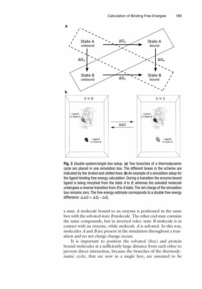
The two branches of a thermodynamic cycle can be combined into a single transition by performing both transitions in the same box. This is important to bear in mind, when an alchemical modifi-cation involves a charge change between the states. In such a case, the simulation box in one of the end states carries a non-zero charge, hence, treatment of the electrostatic interactions by means of the Ewald summation introduces artifacts. Meanwhile methods that would not introduce such artifacts, e.g. a simple cut-off based Coulomb interaction calculation, are generally less accurate. Hence, the best solution is to design a specific simulation setup to keep the system neutral at all times during a transition. One such simulation setup is to combine both branches of a thermodynamic cycle in one simulation box (Fig. 3). In such a double-system/single- box setup,

Fig. 2 Schematic representation of a thermodynamic cycle. To determine the change in binding affinity upon a protein mutation or ligand modification, the difference between the binding free energy of the ligand or protein in state A (ΔG1) and that of the state B (ΔG2) need to be determined. However, the values (ΔG3) and (ΔG4) are more accessible to the free energy perturbation methods. Using the conservation of energy in this closed cycle, we can derive DD D D D DG G G= - = -2 1 4G G3


189

a state A molecule bound to an enzyme is positioned in the same box with the solvated state B molecule. The other end state contains the same compounds, but in inverted roles: state B molecule is in contact with an enzyme, while molecule A is solvated. In this way, molecules A and B are present in the simulation throughout a tran-sition and no net charge change occurs.

It is important to position the solvated (free) and protein bound molecules at a sufficiently large distance from each other to prevent direct interaction, because the branches of the thermody-namic cycle, that are now in a single box, are assumed to be

Fig. 3 Double-system/single-box setup. (a) Two branches of a thermodynamic cycle are placed in one simulation box. The different boxes in the scheme are indicated by the broken and dotted lines. (b) An example of a simulation setup for the ligand binding free energy calculation. During a transition the enzyme bound ligand is being morphed from the state A to B, whereas the solvated molecule undergoes a reverse transition from B to A state. The net charge of the simulation box remains zero. The free energy estimate corresponds to a double free energy difference: ΔΔG = ΔG4 −ΔG3


190

independent. In practice, placing the structures ∼ 3 nm apart is suf-ficient to obtain accurate free energy estimates. To prevent an interaction between the solvated molecule and the protein due to motions during the simulation, a position restraint on a single atom of the molecule free in solution can be imposed. Once a sys-tem is set up this way, the estimated free energy corresponds to the ΔΔG of binding.

Even if a charge changing mutation/modification is set up to remain in a neutral simulation box during an alchemical transi-tion, some unwanted electrostatic artifacts may persist due to the finite size and periodicity effects [62].

5 Validation Using Closed Thermodynamic Cycles

To achieve accurate and valuable free energy estimates from simu-lations, it is important to aim at the best possible setup within the approximations made. If and when available, known experimental results can be used to validate a particular setup but even then, there can be multiple reasons for a discrepancy between experiments and simulations. For instance, it is often difficult to completely match experimental conditions with simulation conditions, e.g. trace amounts of a certain ion in the buffer could have a large effect, but are often neglected in simulations. Also, it can never be excluded that there is an error in the experimental results.

From the simulation side the major factors affecting the accu-racy of the results are conformational sampling and the Hamiltonian/force field. One can validate the setup independent of external factors such as the force field or known experimental results, by uti-lizing closed thermodynamic cycles where all transition branches are accessible and are explicitly computed. The result of summing up all branches should then be zero. Any deviation from zero gives access to the accuracy of the approach used. The simplest type of a closed cycle is using the double-system/single-box setup (see Subheading 4), where in one box A2B and B2A are present. A2B can be the transi-tion of one amino acid to another in the case of protein binding, or can be the change from one ligand to another in the case of ligand binding.

The double system in a single box approach is used in the follow-ing example to obtain a closed cycle. A transition from leucine to alanine (L2A) is combined with the reverse transition from alanine to leucine (A2L) in a single system. Ten independent equilibrium simulations of 10 ns are launched and convergence is verified as a function of the number of independent trajectories involved in computing the free energy. Using more independent simulations reduces the error bar. Note that using only one 10 ns trajectory can produce a result that is close to zero, but the error bar is large. In this case, an additional 10 ns of simulation can increase the


191

deviation from zero, but thereby indicates that 10 ns of sampling is not sufficient for the simulation to converge. Combining all ten simulations results in a small error bar (with zero within).

Thus, using short simulation times may often result in seem-ingly good results for closed thermodynamic cycles, since in that case all simulations stay close to the starting structure and the conformational space is insufficiently explored. Assuming that sufficient exploration of the conformational space is required, using longer simulations would be preferred. However, using lon-ger simulations also holds the risk that they will get trapped in artificial minima caused by force field artifacts. To avoid this we recommend using multiple short simulations as done in this exam-ple. This approach ensures better sampling and reduces the risk of getting trapped in artificial minima. Furthermore, a more rigorous and straightforward error estimation could be performed using this approach, provided that a sufficient number of transitions is achieved for each independent simulation. In such a case the free energy can be calculated for each trajectory separately and the error can be evaluated for the deviation among the independent ΔG estimates.

In the example above we used a convenient double-system/ single-box setup. However, in case of a closed cycle is constructed by considering the branches of a thermodynamic cycle separately, one additional caveat in terms of topology construction needs to be taken into account. Both single and dual topology procedures mostly involve dummy atoms, and those need to be considered in a closed cycle. A simple thermodynamic cycle, as represented in Fig. 4a, containing three vertices, might end up in a cycle with six vertices (Fig. 4b), and edges containing only dummy transitions that are not easily accessible [40, 41]. In a typical free energy simu-lation one is often interested in the difference between two ΔG values, where the contribution of the dummy atoms cancels out, e.g. in protein thermostability calculations the effect of the dummy atoms is the same in the reference (unfolded) state as in the folded state, or for ligand binding affinities the effect is the same for the ligand in solvent as the ligand bound to a protein. Therefore, one possibility for the construction of a valid closed thermodynamic

Fig. 4 (a) Closed thermodynamic cycle involving three states. (b) Including the effects of the dummy atoms a closed thermodynamic cycle with three states is transformed to one with six states


192

cycle with three vertices, might be by having ΔΔG values at the edges instead of ΔG. As a simpler alternative, the double-system/single-box setup as shown in the example above could be used (Fig. 5).

6 Non-equilibrium Free Energy Calculation Setup

In this section we will outline the main steps of the alchemical non- equilibrium free energy calculation setup. The described protocol is compatible with the ΔG estimation based on both the Jarzynski equality and CFT. In the first step of the procedure, equilibrium ensembles of the system in both end states need to be generated. Afterwards, short transition simulations are performed starting from the structures selected from the equilibrium ensembles. The work performed by the system is calculated by numerically inte-grating the ¶ ¶H / l curves for every transition. Finally, the free energy difference between the two end states is estimated from the accumulated work values.

To create equilibrium ensembles for both end states of a transi-tion, simulations of the system with the hybrid topology (Subheading 3) can be performed by keeping the transition con-trolling variable λ constant at one of the two end states. This has an advantage that structures from the equilibrium simulations can directly be used as starting structures for the transitions. On the

Fig. 5 Results for a double system in a single box, having both L2A and A2L structures in one box. The number of equilibrium simulations of 10 ns used can be read from the x-axis. Each point on the graph consists of 100 non-equilibrium trajectories of 50 ps


193

other hand, if equilibrium ensembles generated without a hybrid topology are already available, they can be re-used, e.g. when the same residue of a protein needs to be mutated to more than one target, or if an alternative method is used to generate the equilib-rium ensemble which is not compatible with the use of hybrid topologies. In these cases, the hybrid topology can be introduced into structures after generating the equilibrium ensembles with a regular (non-hybrid) topology, but it is advisable to perform a short simulation with the hybrid topology prior to a transition, to allow the system to relax.

For the non-equilibrium transitions, a number of structures (from 100 as in published works [35, 48] up to 450 as in the ATP example described later in this chapter) are picked from both equi-librium ensembles. For each of these structures, a short (usually on the order of 50–200 ps) simulation is performed, during which the topology is changed from one state to the other. For more details on the simulation parameters see Note 1.

The generalized force ¶ ¶H / l associated with this transition is calculated and written out by the simulation program.

The work value for each transition can be obtained by numeri-cal integration of the ¶ ¶H / l curves. Then, two histograms are created from all work values associated with transitions in a single direction (Fig. 6). The CGI, BAR, or another method (Subheading 2.4) can be employed to extract the free energy difference from the work distributions.

The computational time necessary to calculate free energy differences using non-equilibrium approach depends on several factors, including first of all the size of the system and the signifi-cance of the change, but also the desired precision. It might be preferable to get fast approximate results in a screening process, while more computational effort would be spent to obtain a precise value for a specific mutation. The quality of the simulation protocol can be validated using closed thermodynamic cycles (Subheading 5), but a closer look at the transition work distributions may also indi-cate how the results can be improved.

As the CFT is based on the assumption that the transition runs start from an equilibrium ensemble, improving the sampling of these ensembles usually yields the greatest improvement to the quality of the result. This is best achieved by running several paral-lel simulations than a single long one as molecular dynamics simu-lations tend to “get stuck” in local energy minima.

The difference in work values between the forward and back-ward transitions is caused by the fact that the simulations are performed in non-equilibrium conditions. The work distributions for forward and backward transitions will be closer to each other the slower the transitions are. Hence, increasing the length of these simulations would improve the result if the work distributions are not properly overlapping.


194

7 Trypsin Inhibitors

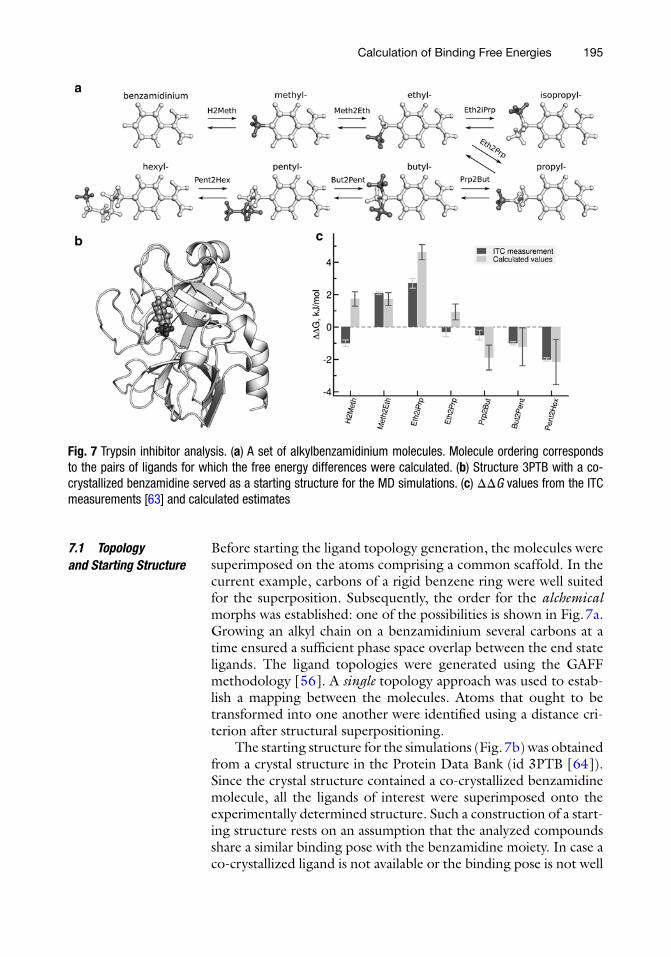
Binding affinity estimation for small organic compounds is of high importance in the search for potential drug candidates. Hence, we will analyze in more detail a study of alchemical ΔΔG calculations for a set of trypsin inhibitors. Talhout et al. [63] performed isother-mal calorimetry (ITC) measurements of the binding free energies for a number of p-n-alkylbenzamidinium molecules. We will use this set of ligands to illustrate the workflow of the alchemical ligand binding free energy calculations, and the ITC measurements will serve us as a reference to assess the quality of our estimates. More information on the computational studies on this set of trypsin inhibitors can be found in the publications [45, 63].

Fig. 6 Non-equilibrium free energy calculation setup. Two equilibrium ensembles are generated (e.g. by MD simulations) for the system in state A and B. From these ensembles, snapshots are selected and used to set up short non- equilibrium transition simulations, in which the state A is turned into B and vice versa


195

Before starting the ligand topology generation, the molecules were superimposed on the atoms comprising a common scaffold. In the current example, carbons of a rigid benzene ring were well suited for the superposition. Subsequently, the order for the alchemical morphs was established: one of the possibilities is shown in Fig. 7a. Growing an alkyl chain on a benzamidinium several carbons at a time ensured a sufficient phase space overlap between the end state ligands. The ligand topologies were generated using the GAFF methodology [56]. A single topology approach was used to estab-lish a mapping between the molecules. Atoms that ought to be transformed into one another were identified using a distance cri-terion after structural superpositioning.

The starting structure for the simulations (Fig. 7b) was obtained from a crystal structure in the Protein Data Bank (id 3PTB [64]). Since the crystal structure contained a co-crystallized benzamidine molecule, all the ligands of interest were superimposed onto the experimentally determined structure. Such a construction of a start-ing structure rests on an assumption that the analyzed compounds share a similar binding pose with the benzamidine moiety. In case a co-crystallized ligand is not available or the binding pose is not well

7.1 Topology and Starting Structure

Fig. 7 Trypsin inhibitor analysis. (a) A set of alkylbenzamidinium molecules. Molecule ordering corresponds to the pairs of ligands for which the free energy differences were calculated. (b) Structure 3PTB with a co-crystallized benzamidine served as a starting structure for the MD simulations. (c) ΔΔG values from the ITC measurements [63] and calculated estimates


196

defined, additional analysis is needed. For example, a molecular docking combined with a long time scale molecular dynamics simu-lation can be used to establish a starting structure with a reliable ligand pose for the alchemical free energy calculations.

The thermodynamic cycle for the binding ΔΔG estimation was constructed by considering the transitions between the two ligand states separately: in water and in contact with trypsin. Such a sim-ple cycle construction was possible, since no charge change was involved in any of the transitions.

Firstly, 10 ns equilibrium molecular dynamics simulations were performed at the end states for the ligands in water and in the bound form. While this time scale does not cover large conforma-tional motions or significant changes in the binding pose, it pro-vides an equilibrium sampling in a free energy minimum close to the starting structure. For the cases, where in a simulation time the system travels far from its initial point, longer sampling times may be required to cover the relevant phase space volume. The non- equilibrium transitions were spawned from the snapshots extracted from the equilibrium trajectories. Here, 100 simulations (50 ps each) were performed going in both directions: A to B and B to A. See also Notes 2 and 3 for more technical details on the equilib-rium sampling and non-equilibrium transitions, respectively.

Integration over the ¶ ¶H / l curves to obtain the work values and subsequent application of the CGI method enabled calculation of the ΔG values for the parts of the thermodynamic cycle: DG A B

water®

and DG A Btrypsin

® (see Note 4). The final ΔΔG estimates are shown in Fig. 7c. A positive value in the graph indicates that the ligand in state B is a weaker binder in comparison with the state A molecule.

For all the ligand pairs the difference between the calculated and experimentally measured free energy values was smaller than 1 kcal/mol. In most cases the ΔΔG values were estimated very accurately, and only the transition from benzamidine to methyl- benzamidine showed a discrepancy of ∼ 1 kT. Larger errors for the estimated free energy differences can be observed for the longer alkyl chains. This effect is a nice illustration of the increased uncer-tainty in the calculated results due to the larger dissipated work values. Alchemically grown longer chains face stronger hindrance and steric clashes, leading to an increase in the amount of work dissipated along the path. The errors could be reduced by per-forming the transitions slower (e.g., 100 ps for a transition).

In the current example the results were presented as the double differences in free energy. In practice, however, an estimate of the ΔG values may be of interest. Conversion from the ΔΔG to the single free energy differences can be attained by setting one of the ΔG estimates to an experimental value (e.g., benzamidinium ITC

7.2 Simulation Setup

7.3 Estimation of the Free Energy Differences


197

measurement) and propagating the differences together with the associated errors along the chain of compounds (Fig. 8). It is clear that the estimates appear far more inaccurate due to the accumula-tion of errors. This result illustrates the importance of an appropriate simulation setup addressing a question of interest. For the case where ΔG estimates are to be compared to the experimental measurements, a single reference structure could be used to create the pairs for tran-sitions. Although the perturbations in such a scenario would be larger than when considering a chain of ligands, the problem of error accu-mulation could be avoided. In addition, such a setup would allow for internal consistency checks via closed thermodynamic cycles.

8 Protein–Protein Binding: Binding of α-Chymotrypsin with Its Inhibitor Turkey Ovomucoid Third Domain

In this example the change in binding free energy upon mutation in the complex of the Kazal-type Ovomucoid from Turkey (OMTKY3) and α-chymotrypsin (CHT) is computed. Leucine 18 of OMTKY3 is mutated to A,I,W,F,Y,V,M,S, and T residues. The results are compared to both experimental data [65] and other theoretical predictions [66]. Note that this example is well suited as a practical hands-on test for the principles learned in this chap-ter. The structure is available in the Protein Data Bank (id 1CHO

Fig. 8 ΔG values calculated by propagating the double free energy differences (ΔΔG) along a chain of ligands (see Fig. 7a) The results are less accurate than the ΔΔG values due to the error accumulation


198

[67]), and calculations can be set up using freely available software (pmx [48] and Gromacs [47]).

The CHT:OMTKY3 complex is shown in Fig. 9, the position (L18) that is mutated is at the interface of the two binding partners. The thermodynamic cycle in Fig. 10 was used to compute the binding free energy. In this cycle the reference is OMTKY3. The shift in binding free energy upon mutation (ΔΔG) is computed from the difference between ΔG1 and ΔG2, since computing the difference between ΔG3 and ΔG4 directly would be computation-ally too expensive.

Fig. 9 The complex of Kazal-type Ovomucoid from Turkey (OMTKY3) and α-chymotrypsin (CHT). Leucine at position 18 is mutated. The structure is taken from the pdb-database (PDB id 1CHO)

Fig. 10 Thermodynamic cycle used for protein–protein binding


199

Setting up these simulations consists of four phases. First the topology is prepared, next the equilibrium simulations are performed, followed by non-equilibrium simulations and finally the results are analyzed to extract the free energy. This procedure is performed for both the complex and for free OMTKY3 in solvent. The topol-ogy is initially prepared using the Gromacs [47] pdb2gmx tool and the Amber99sb [68] force field. Equilibrium simulations of 20 ns are performed for the native protein and all mutants. From those equilibrium simulations, 100 snapshots are selected and hybrid structures and topologies are created using pmx [48] (see Note 5). Those are followed by non-equilibrium transitions of 100 ps each. The free energies are extracted using the BAR method [14] (see Note 4). BAR was used in this case, since the CGI method requires a Gaussian distribution of the work values, which is not always the case for all mutations in this complex. The results of the calculations are shown in Fig. 11. The correlation coefficient with the experiment is 0.83 and the average unsigned error is 7.9 kJ/mol. Particularly, the mutants with the largest desta-bilization are predicted poorly. The same mutations were predicted by Benedix et al. [66], where a slightly better result was obtained, with a correlation coefficient of 0.9 and an average unsigned error of 7.9 kJ/mol.

10 5 0 5 10 15 20 25Experimental binding free energy (kJ/mol)

10

5

0

5

10

15

20

25

30

Calc

ulat

ed b

indi

ng fr

ee e

nerg

y (k

J/mol

)L18A

L18I

L18F

L18M

L18SL18T

L18V

L18W

L18Y

Expected1 kcal/mol dev.2 kcal/mol dev.

Fig. 11 Results of mutations in OMTKY3:CHT complex. The average unsigned error is 7.9 kJ/mol and correlation coefficient is 0.83


200

When comparing to experimental results, their origin has to be taken into account. The experimental results [65] used here are obtained by enzyme assays, where the binding affinity is not mea-sured directly, but instead the inhibition of proteolysis is measured. The inhibition of proteolysis might be related to the binding affinity of OMTKY3, but other factors might play a role, e.g., a certain mutation could trigger a conformational change in CHT which inhibits proteolysis, without having a stronger binding affin-ity than another mutant.

9 ATP and Magnesium Complex in Solution

In the example given here, we show how seemingly simple free energy calculations involving a highly charged ligand (ATP and a bound magnesium) can result in substantial inaccuracies if not treated correctly. Many biological functions require the presence of an ATP molecule which is often only active with a bound magne-sium ion. The binding free energy of an ATP ⋅ Mg complex can be calculated via a thermodynamic cycle where the complex is annihi-lated once from the binding pocket of the protein and once in an unbound (free) state which is represented by an annihilation of the ATP ⋅ Mg in water. The second transformation is in fact the solva-tion free energy. Here, we present some of the pitfalls that might occur merely in the calculation of the solvation free energy of ATP ⋅ Mg, as it presents a challenging system by itself and may be found in much more complex systems as well (e.g., in protein complexes).

The annihilation of an ATP−4 molecule, even when attached to a Mg+2 ion, incorporates a change in the overall system charge which would influence the resulting free energy. One possibility to neu-tralize the system is to add 2 counter Na+ ions that would turn into dummies during the transition as well. However, this effectively turns the free energy of ATP ⋅ Mg solvation, into a combined solva-tion free energy of [ATP ⋅ Mg] + 2Na. Moreover, an issue encoun-tered in equilibrium free energy calculations of this system is that the interaction of the disappearing Na+ ions with the disappearing ATP ⋅ Mg+2 is not sufficiently sampled in the simulated time scales.

A second and more computationally expensive possibility that avoids the coupling of the counter ions to the transition is the double-system/single-box setup (Subheading 4). For this example, one ATP ⋅ Mg complex is annihilated and another is solvated in the same box, while the structures are positioned ∼ 4 nm apart in order to avoid any interaction between them. The Mg+2 ion itself cannot migrate between the ATP molecules when its interactions are turned off, because it is kept close to its respective ATP via a dis-tance restraint. Topology generation is relatively simple, where A

9.1 System Setup: Charged Systems


201

and B states are constructed such that one molecule is present at λ = 0 while the second is annihilated (turned to dummies), and vice versa for λ = 1. This type of setup allows either for directly comput-ing the binding free energy in one simulation box (if the ligand is annihilated while bound to a protein on one side of a box, and solvated on the other side), or to compute a closed cycle as a con-sistency check. In this example we performed the latter.

Having constructed the system as described above, 50 ns equi-librium ensembles were obtained for λ = 0, λ = 1 and, afterwards, fast non-equilibrium transitions were performed 200 ps each. The results are shown in Fig. 12a, indicating that the distributions of the resulting work values do not overlap nor fit into a gaussian function, whereas the estimated ΔG is far from zero.

How is it possible that a transition and its opposite do not result in a zero free energy change? Sampling and symmetry are key issues here. The two ATP ⋅ Mg complexes were found not to be entirely symmetric in the conformations covered by their equilib-rium ensembles. Specifically, it is the Mg+2 ion that adopts different orientations relative to the phosphates of the ATP. In Fig. 12b one can differentiate between two states, which are mutually exclusive for the two ATP molecules in the box: state X, where the Mg+2 is triply coordinated by all three phosphates that adopt a similar dis-tance of 0.3 nm to it, and state Y, where Mg+2 is doubly coordi-nated and found slightly further away from the Pα ( ∼ 0.45 to 0.55 nm). The lower cluster in state Y, where the distance to Pγ

9.2 Calculating a Closed Cycle

Fig. 12 (a) Non-equilibrium free energy calculation of ATP solvation and desolvation which should serve as a closed cycle. The left section of the plot shows the work values as a function of the transition number. Since the transitions are started from consecutive frames it could indicate whether the equilibrium trajectory is drift-ing. The right region of the plot combines the work values into histograms. (b) Distribution of ATP and Mg orientations measured according to distance from Pα and Pγ. Pβ is not shown since its distance does not vary and fluctuates around 0.3 nm


202

shortens, arises from the initial structure, but it gradually equili-brates into the top cluster of state Y within 1–20 ns and never re- visits the former cluster. Since these conformations do not inter-change, they can be seen as two distinct chemical species. Thus, turning one chemical species on, and another off does not represent two opposite reactions and will not converge to ΔG = 0.

Spontaneous transitions between these conformations do not occur in MD simulations with a length of 100 ns, and they are kept separated by a steep barrier. However, the barrier is solely maintained by the highly attractive Coulomb interactions between the phosphates and the magnesium. Since the free energy is a state function, the path from the fully solvated to annihilated (uninteracting dummies) state could be chosen to pass through a reduced charge state, where the charge on the magnesium ion is scaled to +1, while the charge on the phosphate groups is scaled in reverse to maintain the neutrality of the system. This effectively creates two transitions that need to be calculated: one from a fully appeared and fully charged state to a reduced charge state, and then another one into dummies.

To enable the convergence of the closed cycle of annihilating and solvating an ATP ⋅ Mg complex in solution, the calculation is decomposed further into the two ATP orientations, such that tran-sitions (annihilation or solvation) will be performed for each orien-tation (X and Y ) of the ATP1 as depicted by the horizontal arrows in Fig. 13. There is no need to compute the vertical transitions, but we would like to note that both vertical transitions maintain a ΔG ∼ 0. In the reduced charge state, conformations X and Y inter-change multiple times, while they are equally populated. As for the dummy state, the difference between X and Y is merely a difference of orientation in space, which is imposed by a distance restraint.

The distribution of work values for each of the four horizontal transitions shown in Fig. 13 is plotted in Fig. 14. These transitions are as before, performed in both directions to close a thermody-namic cycle. Four hundred and fifty transitions were performed in

1 Distance restraints on the Pα, Pγ and the Mg+2 will keep the atoms in their

respective orientation in one of the two top clusters shown in Fig. 12b.

Fig. 13 An extended closed cycle of an ATP ⋅ Mg complex annihilated and solvated in solution. The horizontal arrows are performed in both directions simultaneously for a closed cycle consistency check


each direction, their length was increased to 2 ns. Indeed, this time the resulting ΔG values are mostly within 1.5 kJ/mol away from zero2, except for the last transition (reduced charge state into dum-mies in state Y ). This state is much more flexible than its fully charged version, and might need more time to converge, i.e. via longer equilibrium simulations, however, electrostatic artifacts could remain due to the nature of the mutation (turning off a charge) and the finite size of the system. In principle, determining whether the generated equilibrium ensemble is indeed at equilib-rium is difficult. However, sometimes examining the series of work values taken from consecutive initial snapshots from the equilib-rium ensemble may indicate whether there is a drift and whether more equilibration time is needed. For example, if we would only have a quarter of the equilibrium trajectory of state X + +2 1to and the corresponding transitions (first 120 transitions in Fig. 14), the drift in work values might have hinted at a trajectory drift, but further equilibration and transitions from later snapshots show that those work values are reproduced again and again.

2 A shorter transition time of 200 ps also gave a result that was fairly close to

zero, but longer times were used to reduce the error.

Fig. 14 Results from non-equilibrium transitions as depicted by the horizontal arrows in Fig. 13. The snapshot number represents the transitions

204

Having arrived at a consistent zero free energy change for a closed cycle of ATP in solution, one can be more confident in the accuracy of ATP ⋅ Mg annihilation in protein complexes. For practi-cal purposes, a similar conformation decomposition can be done when computing the binding free energy of an ATP ⋅ Mg complex in a protein. As indicated earlier, in such a case, the box will contain ATP ⋅ Mg and a protein with ATP ⋅ Mg in its binding pocket which will be simultaneously turned on and off. This time, rather than receiving a zero from each transition (and an overall zero from ATP ⋅ Mg annihilation and resolvation in both orientations), the combined transition from a fully charged state to a dummy state would yield the binding free energy of ATP ⋅ MgX and ATP ⋅ MgY . It can then be combined using the following formula [69]:

D D DG G GX Y= - - + --b b b1 ln[exp( ) exp( )] (24)

10 Notes

1. In the Gromacs simulation package the free energy code is activated by setting the flag free-energy=yes in a molecu-lar dynamics parameter (mdp) file. Triggering this option auto-matically enables the ¶ ¶H / l output to an external file. The initial state of a system is set by defining init-lambda to be equal to 0 or 1 for the states A and B, respectively. Setting the two aforementioned parameters is sufficient to perform an equilibrium sampling simulation at one of the end states. For the transition runs, an increment in λ needs to be specified by setting the parameter delta-lambda to a non-zero value. delta-lambda has to be estimated such that an end state is

Table 1 Parameters and suggested values for the non-equilibrium free energy calculations

Parameter Value

init-lambda 0 or 1

delta-lambda (equilibration) 0

delta-lambda (transition) ±1/nsteps

nstdhdl 1

sc-coul yes

sc-alpha 0.3

sc-sigma 0.25

sc-power 1


205

reached within the defined number of integration steps. For example, for a transition from init-lambda=1 to the end state λ = 0 in 50 ps with an integration time step of 2 fs, 25,000 integration steps are required. Hence, delta-lambda has to be set to −4e−5. For the non-equilibrium free energy calcula-tion it is important to collect all the available ∂H ∕ ∂ λ values, therefore, the frequency of output should not be reduced, i.e. nstdhdl=1. We recommend using the soft-core potential energy function for both the van der Waals and electrostatic interactions. Table 1 summarizes the essential parameters for the non-equilibrium free energy calculations as defined in Gromacs. The suggested values should be adjusted to a par-ticular problem at hand.

2. The equilibration simulations at the end states (λ = 0 and λ = 1) are performed following the standard unbiased molecular dynamics simulation setup. If the hybrid topology for a system is generated, the free energy code must be switched on and the λ state has to be defined (see Note 1). It is also important to consider which ensemble, canonical or NPT, is sampled, since on this choice depends which free energy will be calculated—Helmholtz or Gibbs. Dispersion correction for the energy and pressure has a significant effect on the accuracy of estimated free energies [70, 71] (simulation parameter in Gromacs DispCorr=EnerPres).

3. When setting up non-equilibrium free energy simulations, three parameters concerning the simulation length need to be decided upon. Firstly, the length of an equilibrium sampling simulation has to be defined. The time dedicated for this step very much depends on a particular system at hand, and on the time scale of conformational changes: an equilibration may vary from a nanosecond to microsecond range. Secondly, the number of spawned non-equilibrium transitions needs to be chosen. The starting structures, with the associated velocities, need to cover the sampled equilibrium ensemble. In practice, 100 transitions in each direction are often sufficient to reach a converged free energy estimate. The third parameter, the time spent for a single transition, depends on the scale of perturba-tion between the states A and B. Extending the time from 50 ps up to several nanoseconds per simulation will improve convergence, as for the slower transitions less work will be dis-sipated. A convenient method to assess the convergence is by monitoring the extent of an overlap between the work distri-butions for the forward and backward transitions: for the larger overlap free energy estimate is more accurate. While the sec-ond and third parameters are responsible for the convergence and statistical error of the free energy estimate, it is the equili-bration time which mostly contributes to the accuracy of the ΔΔG estimate.


206

4. The work required for a transition is obtained by numerically integrating the ¶ ¶H / l curves. It is important to bear in mind that the integration ranges for the forward transition are defined to be 0 and 1, not to confuse them with the actual simulation time (which is, e.g., reported in the Gromacs ¶ ¶H / l output). For the reverse transition integration from 1 to 0 has to be per-formed and afterwards the sign of the work value needs to be inverted (see Eq. 17 in Subheading 2.4). This effectively allows integration from 0 to 1 without the subsequent sign inver-sion for the reverse transition. The pmx [48] package contains the script (analyze_crooks.py) performing the integration using Gromacs ¶ ¶H / l output directly for an arbitrary number of for-ward and reverse trajectories. Estimate of the free difference using the CGI approach (Eq. 19) or BAR (Eq. 20) can also be obtained with analyze_crooks.py in the pmx package.

5. The hybrid topology for an amino acid mutation can be created employing the pre-generated mutation database available in the pmx package. Firstly, the hybrid structural file containing atoms of both states needs to be generated (script mutate.py). In the second step, the standard topology generation is performed using the newly created structure file (pdb2gmx in Gromacs). As the hybrid structure (e.g., A2L amino acid denoting alanine in state A and leucine in state B) is not pres-ent in the standard biomolecular force fields, one needs to use the specifically modified force field files provided in the pmx. Finally, the parameters for the B state of the system need to be added to the topology file. This can be accomplished with the make_bstate.py script from the pmx package.

References

1. Torrie GM, Valleau JP (1977) Nonphysical sampling distributions in Monte Carlo free- energy estimation: umbrella sampling. J Comput Phys 23(2):187–199

2. Kirkwood JG (1935) Statistical mechanics of fluid mixtures. J Chem Phys 3:300–313

3. Ben-Naim A (1992) Statistical thermodynamics for chemists and biochemists. Plenum Press, New York

4. Chipot C, Pohorille A (eds) (2007) Free energy calculations. Theory and applications in chemistry and biology. Springer series in chem-ical physics, vol 86

5. Christ CD, Mark AE, van Gunsteren WF (2010) Basic ingredients of free energy calculations: a review. J Comput Chem 31(8):1569–1582. ISSN 1096-987X. doi:10.1002/jcc.21450. http://dx.doi.org/10.1002/jcc.21450

6. Michael S, David M (2013) An introduction to best practices in free energy calculations. In: Biomolecular simulations: methods and proto-cols. Methods in molecular biology, vol 924. Humana Press, New York, pp 271–311

7. Zwanzig RW (1954) High-temperature equation of state by a perturbation method. I. Nonpolar gases. J Chem Phys 22: 1420–1426

8. Pohorille A, Jarzynski C, Chipot C (2010) Good practices in free-energy calculations. J Phys Chem B 114(32):10235–10253

9. Landau LD (1938) Statistical physics. The Clarendon Press, Oxford

10. Lu N, Kofke DA (2001) Accuracy of free- energy perturbation calculations in molecular simulation. I. Modeling. J Chem Phys 114: 7303–7311


207

11. Lu N, Kofke DA (2001) Accuracy of free- energy perturbation calculations in molecular simulation. II. Heuristics. J Chem Phys 115: 6866–6875

12. Shirts MR, Pande VS (2005) Comparison of efficiency and bias of free energies computed by exponential averaging, the Bennett accep-tance ratio, and thermodynamic integration. J Chem Phys 122(14):144107-1–144107-16

13. Bennett CH (1976) Efficient estimation of free energy differences from Monte Carlo data. J Comput Phys 22(2):245–268

14. Shirts MR, Bair E, Hooker G, Pande VS (2003) Equilibrium free energies from nonequilibrium measurements using maximum- likelihood methods. Phys Rev Lett 91(14):140601

15. Mezei M (1992) Polynomial path for the calcu-lation of liquid state free energies from computer simulations tested on liquid water. J Comput Chem 13(5):651–656

16. Steinbrecher T, Mobley DL, Case DA (2007) Nonlinear scaling schemes for Lennard-Jones interactions in free energy calculations. J Chem Phys 127:214108

17. Kumar S, Rosenberg JM, Bouzida D, Swendsen RH, Kollman PA (1992) The weighted histo-gram analysis method for free-energy calcula-tions on biomolecules. I. The method. J Comput Chem 13(8):1011–1021

18. Shirts MR, Chodera JD (2008) Statistically optimal analysis of samples from multiple equi-librium states. J Chem Phys 129:124105

19. Shenfeld DK, Xu H, Eastwood MP, Dror RO, Shaw DE (2009) Minimizing thermodynamic length to select intermediate states for free- energy calculations and replica-exchange simu-lations. Phys Rev E 80(4):046705

20. Buelens FP, Grubmüller H (2012) Linear- scaling soft-core scheme for alchemical free energy calculations. J Comput Chem 33(1): 25–33

21. Mazor M, Pettitt BM (1991) Convergence of the chemical potential in aqueous simulations. Mol Simul 6(1–3):1–4

22. Mitchell MJ, McCammon JA (1991) Free energy difference calculations by thermody-namic integration: difficulties in obtaining a precise value. J Comput Chem 12(2):271–275

23. Straatsma TP, McCammon JA (1991) Multi-confi guration thermodynamic integration. J Chem Phys 95:1175

24. Jorge M, Garrido NM, Queimada AJ, Economou IG, Macedo EA (2010) Effect of the integration method on the accuracy and computational efficiency of free energy calcula-tions using thermodynamic integration. J Chem Theory Comput 6(4):1018–1027

25. Bruckner S, Boresch S (2011) Efficiency of alchemical free energy simulations. II. Impro-vements for thermodynamic integration. J Comput Chem 32(7):1320–1333

26. Jarzynski C (1997) Nonequilibrium equality for free energy differences. Phys Rev Lett 78(14):2690–2693

27. Cuendet MA (2006) The Jarzynski identity derived from general hamiltonian or non- hamiltonian dynamics reproducing NVT or NPT ensembles. J Chem Phys 125:144109

28. Hummer G (2001) Fast-growth thermody-namic integration: error and efficiency analysis. J Chem Phys 114:7330–7337

29. Gore J, Ritort F, Bustamante C (2003) Bias and error in estimates of equilibrium free- energy differences from nonequilibrium mea-surements. Proc Natl Acad Sci USA 100(22): 12564–12569

30. Crooks GE (1998) Nonequilibrium measure-ments of free energy differences for microscop-ically reversible Markovian systems. J Stat Phys 90(5–6):1481–1487

31. Crooks GE (1999) Entropy production fluc-tuation theorem and the nonequilibrium work relation for free energy differences. Phys Rev E 60(3):2721–2726

32. Chelli R, Marsili S, Barducci A, Procacci P (2007) Recovering the Crooks equation for dynamical systems in the isothermal-isobaric ensemble: a strategy based on the equations of motion. J Chem Phys 126:044502

33. Nanda H, Lu N, Woolf TB (2005) Using non- Gaussian density functional fits to improve rel-ative free energy calculations. J Chem Phys 122(13):134110-1–134110-8

34. Maragakis P, Ritort F, Bustamante C, Karplus M, Crooks GE (2008) Bayesian estimates of free energies from nonequilibrium work data in the presence of instrument noise. J Chem Phys 129:024102

35. Goette M, Grubmüller H (2009) Accuracy and convergence of free energy differences calcu-lated from nonequilibrium switching processes. J Comput Chem 30(3):447–456

36. Bramwell ST, Christensen K, Fortin J-Y, Holdsworth PCW, Jensen HJ, Lise S, López JM, Nicodemi M, Pinton J-F, Sellitto M (2000) Universal fluctuations in correlated sys-tems. Phys Rev Lett 84(17):3744–3747

37. Massey FJ Jr (1951) The Kolmogorov-Smirnov test for goodness of fit. J Am Stat Assoc 46(253):68–78

38. Pearlman DA, Kollman PA (1991) The over-looked bond-stretching contribution in free energy perturbation calculations. J Chem Phys 94:4532–4545


208

39. Pearlman DA (1994) A comparison of alterna-tive approaches to free energy calculations. J Phys Chem 98(5):1487–1493

40. Boresch S, Karplus M (1999) The role of bonded terms in free energy simulations. 2. Calculation of their influence on free energy differences of solvation. J Phys Chem A 103(1):119–136

41. Boresch S, Karplus M (1999) The role of bonded terms in free energy simulations: 1. Theoretical analysis. J Phys Chem A 103(1): 103–118

42. Bash PA, Singh UC, Langridge R, Kollman PA (1987) Free energy calculations by computer simulation. Science 236(4801):564–568

43. Beutler TC, Mark AE, van Schaik RC, Gerber PR, van Gunsteren WF (1994) Avoiding sin-gularities and numerical instabilities in free energy calculations based on molecular simula-tions. Chem Phys Lett 222(6):529–539. ISSN 0009-2614

44. Zacharias M, Straatsma TP, McCammon JA (1994) Separation-shifted scaling, a new scal-ing method for Lennard-Jones interactions in thermodynamic integration. J Chem Phys 100: 9025–9031

45. Gapsys V, Seeliger D, de Groot BL (2012) New soft-core potential function for molecular dynamics based alchemical free energy calcu-lations. J Chem Theory Comput 8(7): 2373–2382

46. Tosco P, Balle T, Shiri F (2011) Open 3DALIGN: an open-source software aimed at unsupervised ligand alignment. J Comput Aided Mol Des 25(8):777–783

47. Hess B, Kutzner C, van der Spoel D, Lindahl E (2008) GROMACS 4: algorithms for highly efficient, load-balanced, and scalable molecular simulation. J Chem Theory Comput 4(3): 435–447

48. Seeliger D, De Groot BL (2010) Protein ther-mostability calculations using alchemical free energy simulations. Biophys J 98(10):2309–2316. ISSN 0006-3495

49. O’Boyle NM, Banck M, James CA, Morley C, Vandermeersch T, Hutchison GR (2011) Open Babel: an open chemical toolbox. J Cheminf 3(1):1–14

50. Sadowski J, Gasteiger J, Klebe G (1994) Comparison of automatic three-dimensional model builders using 639 X-ray structures. J Chem Inf Comput Sci 34(4):1000–1008

51. Singh UC, Kollman PA (1984) An approach to computing electrostatic charges for molecules. J Comput Chem 5(2):129–145

52. Bayly CI, Cieplak P, Cornell W, Kollman PA (1993) A well-behaved electrostatic potential

based method using charge restraints for deriving atomic charges: the RESP model. J Phys Chem 97(40):10269–10280

53. Jakalian A, Bush BL, Jack DB, Bayly CI (2000) Fast, efficient generation of high-quality atomic charges. AM1-BCC model: I. Method. J Comput Chem 21(2):132–146

54. Mobley DL, Dumont É, Chodera JD, Dill KA (2007) Comparison of charge models for fixed- charge force fields: small-molecule hydration free energies in explicit solvent. J Phys Chem B 111(9):2242–2254

55. Wang J, Wang W, Kollman PA, Case DA (2006) Automatic atom type and bond type perception in molecular mechanical calcula-tions. J Mol Graph Model 25(2):247–260

56. Wang J, Wolf RM, Caldwell JW, Kollman PA, Case DA (2004) Development and testing of a general amber force field. J Comput Chem 25(9):1157–1174

57. Vanommeslaeghe K, Hatcher E, Acharya C, Kundu S, Zhong S, Shim J, Darian E, Guvench O, Lopes P, Vorobyov I, MacKerell AD Jr (2010) CHARMM general force field: a force field for drug-like molecules compatible with the CHARMM all-atom additive biological force fields. J Comput Chem 31(4):671–690

58. Vanommeslaeghe K, MacKerell AD Jr (2012) Automation of the CHARMM General Force Field (CGenFF) I: bond perception and atom typing. J Chem Inf Model 52(12): 3144–3154

59. Vanommeslaeghe K, Raman EP, MacKerell AD Jr (2012) Automation of the CHARMM General Force Field (CGenFF) II: assignment of bonded parameters and partial atomic charges. J Chem Inf Model 52(12):3155–3168

60. Malde AK, Zuo L, Breeze M, Stroet M, Poger D, Nair PC, Oostenbrink C, Mark AE (2011) An automated force field topology builder (ATB) and repository: version 1.0. J Chem Theory Comput 7(12):4026–4037

61. Ribeiro AAST, Horta BAC, de Alencastro RB (2008) MKTOP: a program for automatic con-struction of molecular topologies. J Braz Chem Soc 19(7):1433–1435

62. Rocklin GJ, Mobley DL, Dill KA, Hünenberger PH (2013) Calculating the binding free ener-gies of charged species based on explicit-sol-vent simulations employing lattice-sum methods: an accurate correction scheme for electrostatic finite-size effects. J Chem Phys 139(18):184103.

63. Talhout R, Villa A, Mark AE, Engberts JBFN (2003) Understanding binding affinity: a combined isothermal titration calorimetry/molecular dynamics study of the binding of a


209

series of hydrophobically modified benzami-dinium chloride inhibitors to trypsin. J Am Chem Soc 125(35):10570–10579

64. Marquart M, Walter J, Deisenhofer J, Bode W, Huber R (1983) The geometry of the reactive site and of the peptide groups in trypsin, trypsinogen and its complexes with inhibitors. Acta Crystallogr Sect B Struct Sci 39(4):480–490

65. Lu W, Apostol I, Qasim MA, Warne N, Wynn R, Zhang WL, Anderson S, Chiang YW, Ogin E, Rothberg I, Ryan K, Laskowski M (1997) Binding of amino acid side-chains to S1 cavities of serine proteinases. J Mol Biol 266(2): 441–461

66. Benedix A, Becker CM, de Groot BL, Caflisch A, Böckmann RA (2009) Predicting free energy changes using structural ensembles. Nat Methods 6(1):3–4

67. Fujinaga M, Sielecki AR, Read RJ, Ardelt W, Laskowski M, James MNG (1987) Crystal and molecular structures of the complex of α-chymotrypsin with its inhibitor turkey ovo-mucoid third domain at 1.8 Å resolution. J Mol Biol 195(2):397–418

68. Hornak V, Abel R, Okur A, Strockbine B, Roitberg A, Simmerling C (2006) Comparison of multiple Amber force fields and develop-ment of improved protein backbone parame-ters. Proteins Struct Funct Bioinform 65(3): 712–725

69. Mobley DL, Chodera JD, Dill KA (2006) On the use of orientational restraints and symme-try corrections in alchemical free energy cal-culations. J Chem Phys 125(8):084902. doi: 10.1063/1.2221683. http://link.aip.org/link/?JCP/125/084902/1

70. Shirts MR, Pitera JW, Swope WC, Pande VS (2003) Extremely precise free energy calcula-tions of amino acid side chain analogs: com-parison of common molecular mechanics force fields for proteins. J Chem Phys 119(11): 5740–5761

71. Shirts MR, Mobley DL, Chodera JD, Pande VS (2007) Accurate and efficient corrections for missing dispersion interactions in mole-cular simulations. J Phys Chem B 111(45): 13052–13063


Calculation of Binding Free Energies - Max Planck Society · PDF filefree energies are among...

Documents

Transcript of Calculation of Binding Free Energies - Max Planck Society · PDF filefree energies are among...