CALCULATION OF ACID GAS DENSITY IN THE VAPOR, … · CALCULATION OF ACID GAS DENSITY IN THE VAPOR,...

______________________________________________________________________________ Boyle and Carroll 1

© 2001

CALCULATION OF ACID GAS DENSITY IN THE VAPOR,LIQUID, AND DENSE-PHASE REGIONS

Tim B. BoylePanCanadian Petroleum Ltd.

150 - 9 Avenue SWCalgary, Alberta T2P 1S2

John J. CarrollGas Liquids Engineering Ltd.#300, 2749 - 39 Avenue NECalgary, Alberta T1Y 4T8

Acid gas injection has quickly become the method of choice for the disposal of unwanted acid

gas (hydrogen sulfide and carbon dioxide). This is especially true if the quantity of acid gas is

small. One of the important parameters in the design of an injection scheme is the density of the

acid gas mixture.

This paper reviews the available experimental data for the densities of these mixtures and

compares several methods for calculating the density. The first element of the study will be an

investigation of the density predictions for pure hydrogen sulfide and carbon dioxide where a

substantial amount of data exists. Next the binary mixture will be examined. For the binary

mixture only a limited amount of data are available.

In acid gas injection the range of temperature of interest is from 0° to 150°C and

pressures from about atmospheric up to 30 MPa. This range of conditions includes the vapor,

liquid, and dense-phase regions. It is therefore important that the model be able to predict the

density in all three regions. This study focuses on the ability of the common cubic equations of

state (Soave-Redlich-Kwong [SRK], Peng-Robinson [PR], and Patel-Teja [PT]) to predict the

densities. Also, the effect of volume shifting on the SRK and PR equations is examined.

Of the six equations examined in this study, only the SRK was deemed to be

unsatisfactory for predicting densities over the entire range of conditions. The errors for this

equation were often larger than 10%. The volume-shifted SRK is marginally satisfactory. The

volume-shift dramatically improves the density in the liquid region, but not in the supercritical

region. The other four equations (PR, two volume shifted PR, and PT) exhibited errors less than

10% except in the near critical region.


© 2001

INTRODUCTION

Acid gas, a mixture of carbon dioxide and hydrogen sulfide, is a byproduct of natural gas

sweetening processes. The acid gas mixture is toxic and environmentally problematic so it must

be dealt with appropriately. If there is a large quantity of acid gas, the hydrogen sulfide contained

therein is typically converted to elemental sulfur using a Claus process. In this process the carbon

dioxide is usually released to the atmosphere.

Acid gas injection has become an economical way to deal with small quantities of acid

gas. Furthermore, acid gas injection is a very low emission process, typically on a percentage

basis, much lower than a Claus plant. In Western Canada there are about 25 such projects

currently in operation and several more are being planned. In other parts of the world acid gas

injection is starting to be looked upon favorable as a disposal method.

It should be noted that acid gas injection is not limited to small projects. Sulfur prices are

currently very low and the stockpiling of elemental sulfur may not be an option. Limited space

may force sulfur producers to find alternative means for dealing with the acid gas. Thus even

larger producers are looking to acid gas injection as an option to the production of sulfur.

The acid gas injection process is simple in concept. The acid gas comes from the amine

regenerator tower at low pressure (typically less than 200 kPa) and at about 50°C, the

temperature of the overhead condenser. In addition it is saturated water. The gas is compressed

using a multistage compressor. The pressure of the gas must be at least that required for injection

into a deep reservoir. The pressure at the surface is usually substantially less than the reservoir

pressure. This is due to the hydrostatic head of the fluid being injected. Injection pressures

depend upon the injection zone but they may be as large as 15 MPa. Reservoir pressure can be as

high as 30 MPa, and in extreme cases even higher.

One of the key properties in the design of an acid gas injection scheme is the density of

the fluid (Carroll and Lui, 1997; Carroll and Maddocks, 1999). Accurate predictions of the

density are required for the vapor, liquid, and supercritical (dense-phase) regions. This paper will

review the available experimental data for acid gas densities. Several popular methods for

density calculations will be examined.

Density prediction methods that are phase specific will not be examined in this study. For

example, there are several correlations designed for estimating the densities of liquids only (see

Reid et al, 1987). As was just noted, in acid gas injection it is important to be able to predict the


© 2001

density for all fluid phases. It is also important to have a well-behaved function as the fluid

transverses the various phase regions (Carroll and Lui, 1987). Therefore, the liquid density

correlations are less useful for this application, even though they are of high accuracy.

EXPERIMENTAL DENSITIES

The amount of experimental data available for the densities of carbon dioxide and

hydrogen sulfide is quite large. Therefore, instead of reviewing the data in this paper, literature

reviews will be used. These compilations of the pure component properties cover the entire range

of pressure and temperature of interest in this study.

Pure Carbon Dioxide

There is significantly more data available for carbon dioxide than for hydrogen sulfide,

particularly for the transport properties. One reason for this is that carbon dioxide is considerably

easier to deal with than hydrogen sulfide. In addition, carbon dioxide has a much lower critical

point placing this interesting region in a range more accessible to experimenters. The vicinity

near the critical point is attractive to researchers because of the nature of the physical properties

in that region – the properties change dramatically with small changes in either the temperature

or the pressure.

The latest review of the thermodynamic properties of carbon dioxide is that of Span and

Wagner (1996). This investigation is a through and critical review of the available experimental

data. The tables were generated using a highly accurate, but complex, equation of state. The

tabulation of Span and Wagner (1996) will be used here in order to compare model density

predictions.

In addition, Angus et al. (1976) thoroughly reviewed the thermodynamic properties of

CO2 and formulated several tables. Vukalovich and Altunin (1968) reviewed both thermo-

dynamic and transport properties of CO2. Although these data sets are useful, they are not used in

this study as they have been superceded by the newer tables of Span and Wagner (1996).

Pure Hydrogen Sulfide

Goodwin (1983) extensively reviewed the thermodynamic properties of hydrogen sulfide.

Using an advanced equation of state, a table of properties was constructed over a wide range of


© 2001

pressures and temperatures. Hydrogen sulfide density data from Goodwin (1983) will be used in

this study.

As was noted earlier, much less data was used to build the correlation for hydrogen

sulfide than was used for carbon dioxide. Notwithstanding, the tables of Goodwin (1983) are

probably the best currently available for the thermodynamic properties of hydrogen sulfide.

Binary Mixtures

In a study of the phase behavior and volumetric properties of sour gas mixtures,

Robinson et al. (1960) [also see Macrygeorgos (1958)] reported the densities for three mixtures

of carbon dioxide and hydrogen sulfide. These data were for mixtures containing 17.75%,

20.35% and 60.25% hydrogen sulfide at 71.1°C (160°F) and pressures from 1.0 to 12.4 MPa

(150 to 1800 psia). All of these data are in the gaseous region (compressibility factors in the

range 0.95 to 0.45).

In a more thorough investigation of the H2S+CO2 binary system, Kellerman et al. (1995)

measured the densities of four mixtures: 6.07%, 9.55%, 29.33%, and 49.99% hydrogen sulfide.

Temperatures in this study ranged from –23.2° to 176.9°C (-9.7° to 350.3°F) and pressures up to

20.0 MPa (2900 psia) These measurements included both liquid and vapor regions.

The data from both of these sources will be used in this study.

MODELLING ACID GAS DENSITY

Equations of state, and most notably cubic equations of state, have become the models of

choice in the process modeling business. This is particularly true for the simulation of processes

for the treatment of natural gas. Two popular cubic equations are the Soave (1972) modification

of the Redlich-Kwong equation (SRK) and the equation of state of Peng and Robinson (1976)

(PR). The literature is filled with additional modifications of these equations. In fact the

modifications are often implemented under the original names in commercial software packages.

Thus the users of the software should do so with some caution.

The PR and the SRK are classified as two-parameter cubic equations and can show

significant deviations in predicted liquid density when compared to experimental data. Errors are

typically on the order of 5-10%, although larger errors can be expected in the region near a

critical point. Errors specific to acid gases will be presented in more detail later in this paper.


© 2001

Recent attempts at improving liquid densities have employed higher-order equations. For

example, the model by Patel and Teja (1982) (PT) has three parameters, and the model by

Trebble et al. (TBS) has four parameters (Trebble and Bishnoi, 1986; Salim and Trebble, 1991).

These higher-order equations rarely improve the vapor-liquid equilibrium compared to the

predictions from the simpler two-parameter models. Due to their added complexity, they have

yet to gain wide acceptance.

This study focuses on the ability of the PR, SRK and PT equations of state to predict acid

gas density in the vapour, liquid and dense-phase regions. The pure component properties and

binary interaction parameters required as input to the various equations of state are given in

Appendix A. These values were taken from the literature and no attempt was made to optimize

them in order to improve the density predictions. Details of the three equations of state are

summarized in Appendix B.

Density from Equation of State Models

Equations of state relate the temperature, pressure and specific (or molar) volume of a

fluid. Cubic equations of state model the pressure of a fluid as a sum of an attractive and

repulsive term. The equations are therefore in the form P = f(T,v). Rearrangement of the

equations to a volume explicit form produces a cubic (third-order) polynomial. The solution to a

cubic equation result in one real or three real roots (two or all three of which may be equal).

For unsaturated fluids in the sub-critical region only one of the roots, the most

thermodynamically stable, is physically meaningful. For sub-critical saturated fluids two roots of

equal thermodynamic stability are physically meaningful. It is worth noting that high

temperature single-phase fluids may also produce three real roots, one or more being negative.

Negative roots, or specific volume roots less than the co-volume of the equation of state, b (see

Appendix B), are neglected.

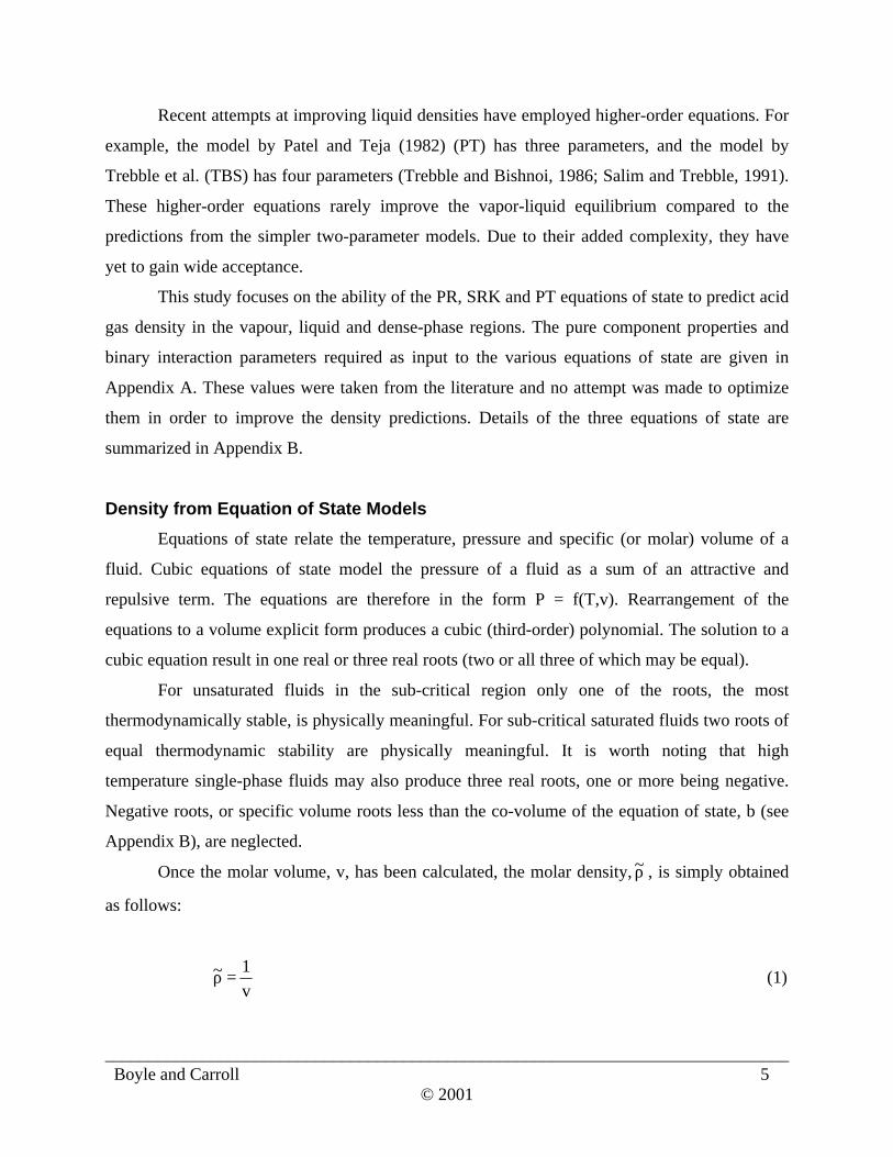
Once the molar volume, v, has been calculated, the molar density, ρ~ , is simply obtained

as follows:

v

1~ =ρ (1)


© 2001

Furthermore, the mass density, ρ, which is the normal definition of the density, is given by:

v

M=ρ (2)

where M is the molar mass (molecular weight) of the fluid.

Volume-Shifting

One method that has become quite popular to improve the density prediction form cubic

equations of state is called volume shifting. In its simplest form, originally proposed by Peneloux

et al. (1982), volume shifting is a correction to the calculated molar volume:

cvv EoScorrected += (3)

where vEoS is the volume estimated from the equation of state and c is the volume-shift

parameter, which in this case is a constant. If the volume shift parameter is properly selected,

then the corrected volume should be an improved estimate of the true molar volume. Peneloux et

al. (1982) suggest fitting the saturated liquid density at Tr = 0.7 to obtain the volume-shift

parameter. Alternatively, the volume-shift parameter could be used as an adjustable parameter,

which is fit by minimizing the error in the density prediction.

To apply this method to mixtures, it is assumed that the c for the mixture, cmix, is the

mole-fraction weighted average of the parameters for the pure components.

∑=

=NC

1i

iimix cxc (4)

where xi is the mole fraction of component i and ci is the volume shift parameter for component

i.

Mathias et al. (1989) noted that the volume-shift method of Peneloux et al. (1982)

improved the prediction of the liquid density only up to reduced temperatures of about 0.85. To


© 2001

improve the prediction over the entire range Mathias et al. (1989) proposed the following

extended correction procedure. They begin with the following equation:

δ+++=

41.0

41.0svv cEoScorrected f (5)

where s is a volume-shift parameter and it is a constant, and δ, the bulk modulus, is a

dimensionless parameter which is defined as follows:

T

2

v

P

RT

v

∂∂

−=δ (6)

where R is the universal gas constant, T is the absolute temperature, and P is the total pressure.

This expression can be evaluated from the equation of state. Finally the function, fc, was chosen

such that the volume shifting procedure calculated the true critical point. For the PR equation,

this function is given by the following expression:

( )s3.946bv c +−=cf (7)

where b is the co-volume from the equation of state.

For mixtures they used the usual, simple mixing rule:

∑=

=NC

1i

iimix sxs (8)

Others have proposed making the volume shift parameter other functions of the

temperature. This adds to the complexity of the model. In addition, a poorly constructed

temperature-dependence can lead to thermodynamic consistency problems (for example, see

Monnery et al., 1998).


© 2001

For the purposes of this study only the corrections proposed by Peneloux et al. (1982) and

Mathias et al. (1989) will be examined. The values of c and s for carbon dioxide and hydrogen

sulfide used in this study are listed in Appendix A.

DISCUSSION

A total of six density calculation methods will be examined in this paper: 1. The original

SRK, 2. The SRK with a Peneloux-type volume shift, 3. The original Peng-Robinson equation, 4.

The PR equation with a Peneloux-type volume shift, 5. The PR equation with a Mathias-type

volume shift, and 6. The PT equation. A complete list of parameters used in this study is

presented in Appendix A.

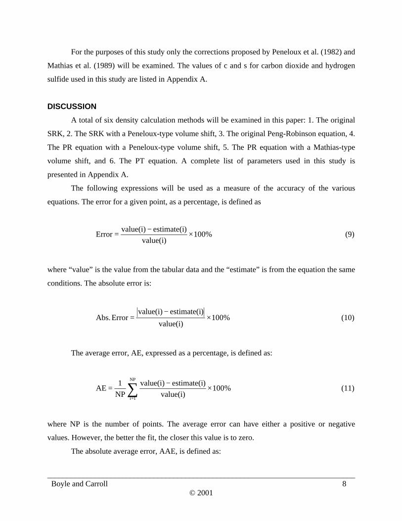
The following expressions will be used as a measure of the accuracy of the various

equations. The error for a given point, as a percentage, is defined as

%100value(i)

)estimate(ivalue(i)Error ×

−= (9)

where “value” is the value from the tabular data and the “estimate” is from the equation the same

conditions. The absolute error is:

%100value(i)

)estimate(ivalue(i)Error Abs. ×

−= (10)

The average error, AE, expressed as a percentage, is defined as:

%100value(i)

)estimate(ivalue(i)

NP

1AE

NP

1i

×−

= ∑=

(11)

where NP is the number of points. The average error can have either a positive or negative

values. However, the better the fit, the closer this value is to zero.

The absolute average error, AAE, is defined as:


© 2001

%100value(i)

)estimate(ivalue(i)

NP

1AAE

NP

1i

×−

= ∑=

(12)

The difference between the AE and the AAE is that in the average error positive and negative

errors tend to cancel each other, which makes the prediction look better than it may actually be.

The average absolute error can only have a positive value, because of the absolute value

function. It is a better indication of the “goodness of fit” than is the average error. A small AE

and a relatively large AAE usually indicates a systematic deviation between the function (values)

and the predictions (estimates).

Finally the maximum error, MaxE, is:

=×

−= NP,...,2,1i%,100

value(i)

)estimate(ivalue(i)MaxE maximum (13)

The maximum error gives the largest deviation of the model from the data values.

There are other methods for estimating the error of a model, but these are sufficient for

our purposes.

Pure Components

The errors for the various density prediction methods will be discussed in six regions.

The six regions are detailed in Table 1.

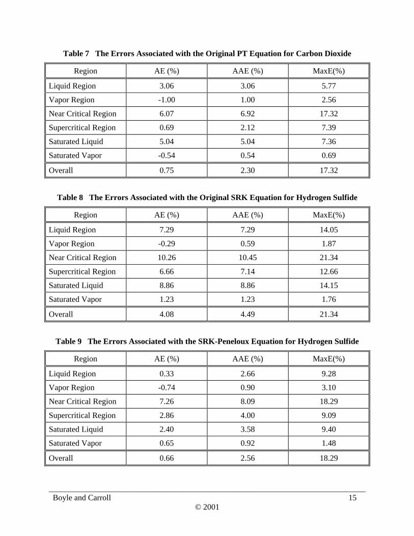
Tables 4 through 7 list the errors for the six equations for predicting the density of pure

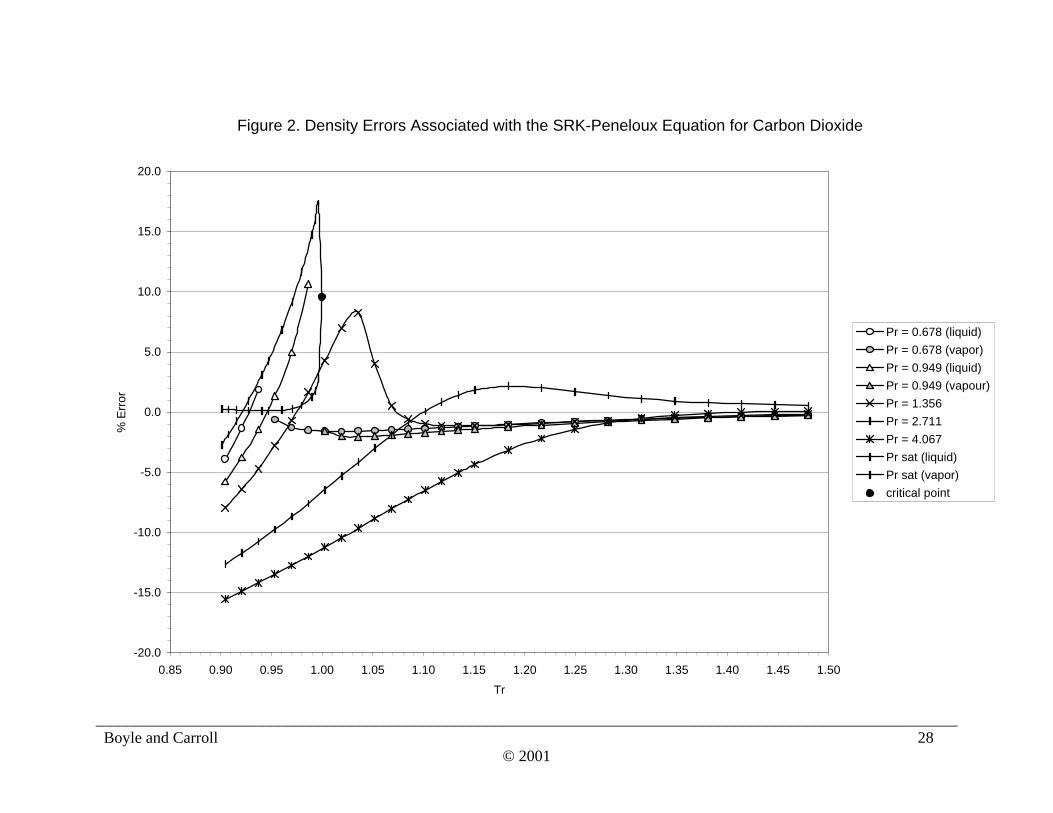
carbon dioxide and Tables 8 through 13 are similar listings for pure hydrogen sulfide. Figures 1

through 6 display a portion of the carbon dioxide error data for each equation over various

regions. Figures 7 through 12 show similar data for hydrogen sulfide.

From these tables and figures it can be observed that the density predictions from the

SRK equation are unsatisfactory. Although the overall average error is only about 5% the

maximum errors often exceed 15% and not only in the near critical region.

The PR equation is better at predicting the densities of these components than is the SRK

equation, which is as expected. For H2S the PT equation is a further improvement over the PR


© 2001

equation, again as expected. However for CO2 the PT equation does not improve the density

predictions over the PR equation. As a check that the implementation of the PT was correct cζ

was set to 0.3074, which reduces the PT equation to the PR equation. The calculated results

obtained for this form of the PT equation were identical to those from the PR.

In all cases the volume-shifting results in an improvement in the predicted liquid density.

However, overall, volume shifting does not always result in an improvement. For example, for

carbon dioxide, the density predictions with the Peneloux-type volume shift of the PR equation

actually are worse than the original PR equation. The reason for this is because the volume-

shifting results in worse predictions of the vapor density.

Mixtures

Table 14 shows the errors for predicting the data from Robinson et al. (1960). Since these

data are only for the vapor phase they were not divided into regions for analysis. In general the

errors for these mixtures are relatively small although a few points have larger errors.

The data set of Kellerman et al. (1995) is sufficiently large that it was examined in three

regions and the definitions of these three regions are given in Table 15. The errors for the six

equations are then summarized in Tables 16 through 21. Figures 13, 14, and 15 are plots of the

errors for the predictions from the six equations for the various mixtures.

In general the observations for the pure components hold true for the binary mixture data.

For example, the density predictions from the SRK equation are unsatisfactory.

The PR equation predicts the mixture data with acceptable accuracy – the maximum error

is less than 10%. Although the volume-shift methods improve the predictions for the liquid

density, overall the density predictions are only marginally improved.

Finally, the PT equation is an improvement over the PR equation when you consider the

overall errors. However, the maximum error for the PT equation is approximately equal to that

for the PR.

CONCLUSIONS

Based on the results presented here is fair to conclude that the original SRK equation is

not sufficiently accurate for predicting the density of acid gas. Although the average errors are

acceptable, the maximum errors in the various regions exceed 10%.


© 2001

The Peneloux-type volume shifting improves this equation significantly. For the pure

components, only in the near critical region do the errors exceed 10%. For the mixture data the

maximum errors are typically less than 11%.

The original PR equation is quite accurate for predicting the densities of the pure

components. Overall the average error for both the pure components is less than about 5% and

for the mixtures is less than about 10%. Only in the near critical region do the errors exceed

10%.

Volume-shifting of the PR equations also tends to improve the density predictions in the

liquid region. The predictions from the Peneloux-type volume shift have an overall error of about

2.5% and the errors from the Mathias-type are less than 2%.

The PT equation, although somewhat more complex, does not result in significant

improvement in the density calculations.

The observations for the pure components are basically the same for the mixtures

examined. The SRK is unsatisfactory for predicting the density of these mixtures. The other five

equations of state and modifications are all sufficiently accurate for engineering calculations,

except in the region near a critical point.

REFERENCES

Angus, S., B. Armstrong, and K.M. de Reuck, International Thermodynamic Tables of the FluidState – Carbon Dioxide, Pergamon Press, Oxford, UK (1976).

Carroll, J.J. and D.W. Lui, “Density, phase behavior keys to acid gas injection”, Oil & Gas J., 95(25), 63-72, (1997).

Carroll, J.J. and J. Maddocks, “Design considerations for acid gas injection”, 49th Laurance ReidGas Conditioning Conference, Norman, OK, Feb. 21-24, (1999).

Goodwin, R.D., Hydrogen Sulfide Provisional Thermophysical Properties from 188 to 700 K atPressure to 75 MPa, Report No. NBSIR 83-1694, National Bureau of Standards, Boulder,CO, (1983).

Haar, L., J.S. Gallagher, and G.S. Kell, NBS/NRC Steam Tables, Hemisphere, Washington, DC(1984).

Kellerman, S.J., C.E. Stouffer, P.T. Eubank, J.C. Holste, K.R. Hall, B.E. Gammon, and K.N.Marsh, Thermodynamic Properties of CO2 + H2S Mixtures, GPA Research Report RR-141,Tulsa, OK, (1995).


© 2001

Knapp, H., R. Döring, L. Oellrich, U. Plöcker, and J.M. Prausnitz, Vapor-Liquid Equilibria forMixtures of Low Boiling Substances, DECHEMA Chemistry Data Series Vol. VI, Frankfurt,Germany, (1982).

Macrygeorgos, C.A., Phase and Volumetric Behavior in the Methane-Carbon Dioxide-HydrogenSulfide System, M.Sc. Thesis, Dept. Chemical Engineering, University of Alberta, Edmonton,AB, (1958).

Mathias, P.M., T. Naheiri, and E.M. Oh, “A density correction for the Peng-Robinson equationof state”, Fluid Phase Equil., 47, 77-87, (1989).

Monnery, W.D., W.Y. Svrcek, and M.A. Satyro, “Gaussian-like volume shifts for the Peng-Robinson equation of state.”, Ind. Eng. Chem. Res., 37, 1663-1672, (1998).

Patel, N.C. and A.S. Teja, “A new cubic equation of state for fluids and fluid mixtures”, Chem.Eng. Sci., 37, 463-473, (1982).

Peneloux, A. E. Rausy, and R. Freze, “A consistent correction for Redlich-Kwong-Soavevolumes”, Fluid Phase Equil., 8, 7-23, (1982)

Peng, D-Y. and D.B. Robinson, “A new two-constant equation of state”, Ind. Eng. Chem. Fund.,15, 59-64, (1976).

Reid, R.C., Prausnitz, J.M. and Poling, B.E., The Properties of Gases & Liquids, 4th ed.,McGraw-Hill, New York, NY, (1987).

Robinson, D.B., C.A. Macrygeorgos, G.W. Govier, “The volumetric behavior of natural gasescontaining hydrogen sulfide and carbon dioxide” Petrol. Trans. AIME, 219, 54-60, (1960).

Salim, P.H. and Trebble, M.A., “A modified Trebble-Bishnoi equation of state: thermodynamicconsistency revisited”, Fluid Phase Equil., 65, 59-71, (1991).

Span, R. and W. Wagner, “A new equation of state for carbon dioxide covering the fluid regionfrom the triple-point temperature to 1100 K at pressure up to 800 MPa” J. Phys. Chem. Ref.Data, 25, 1509-1596, (1996).

Soave, G., “Equilibrium constants from a modified Redlich-Kwong equation of state”, Chem.Eng. Sci., 27, 1197-1203, (1972).

Trebble, M.A. and Bishnoi P.R., “Development of a new four-parameter equation of state”, FluidPhase Equil., 35, 1-18, (1986).

Vukalovich, M.P. and V.V. Altunin, Thermophysical Properties of Carbon Dioxide, Collet’sPublishers Ltd. London, UK, (1968). – translated from Russian.


© 2001

Table 1 Six Regions for Fluid Density Study for the Pure Components

Reduced Temperature Reduced Pressure

1. Liquid Region Tr < 0.95 Pr > Pr(sat)

2. Vapor Region Tr > Tr(sat) Pr < Pr(sat) or Pr < 0.9

3. Near Critical Region 0.95 < Tr < 1.05 0.9 < Pr < 1.5

4. Supercritical Region Tr > 0.95If 0.95 < Tr < 1.05 then Pr > 1.5

If Tr > 1.05 then Pr > 0.9

5. Saturated Liquid Tr = Tr(sat), Tr < 0.95 Pr = Pr(sat)

6. Saturated Vapor Tr = Tr(sat), Tr < 0.95 Pr = Pr(sat)

Table 2 The Errors Associated with the Original SRK Equation for Carbon Dioxide

Region AE (%) AAE (%) MaxE(%)

Liquid Region 13.38 13.38 15.76

Vapor Region 0.49 0.49 2.25

Near Critical Region 13.26 13.26 24.68

Supercritical Region 6.31 6.31 14.30

Saturated. Liquid 15.25 15.25 17.11

Saturated Vapor 2.64 2.64 3.15

Overall 5.41 5.41 24.68

Table 3 The Errors Associated with the SRK-Peneloux Equation for Carbon Dioxide


Liquid Region -2.44 2.83 5.76

Vapor Region -0.66 0.66 1.87


Supercritical Region -1.79 2.49 13.47

Saturated Liquid 0.79 2.05 4.26


Overall -0.90 2.41 17.33


© 2001

Table 4 The Errors Associated with the Original PR Equation for Carbon Dioxide


Liquid Region 2.20 2.20 4.92

Vapor Region -1.09 1.09 2.81




Saturated Vapor -0.84 0.84 1.05

Overall 0.45 2.25 16.66

Table 5 The Errors Associated with the PR-Peneloux Equation for Carbon Dioxide



Vapor Region -1.33 1.33 3.50





Overall -0.93 2.39 14.97

Table 6 The Errors Associated with the PR-Mathias Equation for Carbon Dioxide



Vapor Region -1.46 1.46 4.85

Near Critical Region -0.33 3.93 7.54




Overall -1.21 1.83 7.54


© 2001

Table 7 The Errors Associated with the Original PT Equation for Carbon Dioxide



Vapor Region -1.00 1.00 2.56





Overall 0.75 2.30 17.32

Table 8 The Errors Associated with the Original SRK Equation for Hydrogen Sulfide



Vapor Region -0.29 0.59 1.87





Overall 4.08 4.49 21.34

Table 9 The Errors Associated with the SRK-Peneloux Equation for Hydrogen Sulfide



Vapor Region -0.74 0.90 3.10





Overall 0.66 2.56 18.29


© 2001

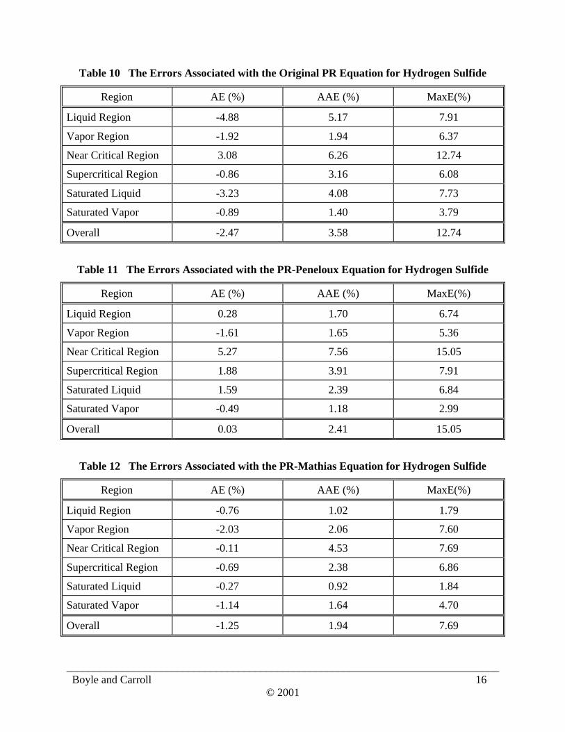
Table 10 The Errors Associated with the Original PR Equation for Hydrogen Sulfide



Vapor Region -1.92 1.94 6.37



Saturated Liquid -3.23 4.08 7.73


Overall -2.47 3.58 12.74

Table 11 The Errors Associated with the PR-Peneloux Equation for Hydrogen Sulfide



Vapor Region -1.61 1.65 5.36





Overall 0.03 2.41 15.05

Table 12 The Errors Associated with the PR-Mathias Equation for Hydrogen Sulfide



Vapor Region -2.03 2.06 7.60

Near Critical Region -0.11 4.53 7.69


Saturated Liquid -0.27 0.92 1.84


Overall -1.25 1.94 7.69


© 2001

Table 13 The Errors Associated with the Original PT Equation for Hydrogen Sulfide



Vapor Region -1.10 1.18 3.94





Overall 0.83 2.45 16.94

Table 14 The Errors for The Mixture Data of Robinson et al. (1960)

Equation AE (%) AAE (%) MaxE(%)

SRK 1.96 2.47 14.01

SRK-Peneloux 0.43 1.46 9.23

PR -0.21 1.51 10.86

PR-Peneloux -0.34 1.49 10.44

PR-Mathias -0.87 1.64 13.67

PT 0.01 1.45 10.11

Table 15 Three Regions for Fluid Density Study for the Mixtures

Reduced Temperature Reduced Pressure

1. Liquid Region Tr < 1.0 Pr > Pr(bubble)

2. Vapor Region Tr > Tr(dew) Pr < Pr(dew) or Pr < 1.0

3. Supercritical Region Tr > 1.0 Pr > 1.0


© 2001

Table 16 The Errors Associated with the Original SRK Equation for the Mixture Data ofKellerman et al. (1995)



Vapor Region 0.51 0.51 4.51


Overall 3.54 3.55 18.87

Table 17 The Errors Associated with the SRK-Peneloux Equation for the Mixture Data ofKellerman et al. (1995)



Vapor Region -0.64 0.65 1.86


Overall -2.46 2.64 10.73

Table 18 The Errors Associated with the Original PR Equation for the Mixture Data ofKellerman et al. (1995)



Vapor Region -1.26 1.26 2.99


Overall -1.86 2.27 9.94


© 2001

Table 19 The Errors Associated with the PR-Peneloux Equation for the Mixture Data ofKellerman et al. (1995)



Vapor Region -1.39 1.39 3.22


Overall -2.52 2.68 9.41

Table 20 The Errors Associated with the PR-Mathias Equation for the Mixture Data ofKellerman et al. (1995)



Vapor Region -1.64 1.64 4.88


Overall -3.26 3.28 11.83

Table 21 The Errors Associated with the Original PT Equation for the Mixture Data ofKellerman et al. (1995)



Vapor Region -1.02 1.02 2.48


Overall -1.11 1.82 10.56


© 2001

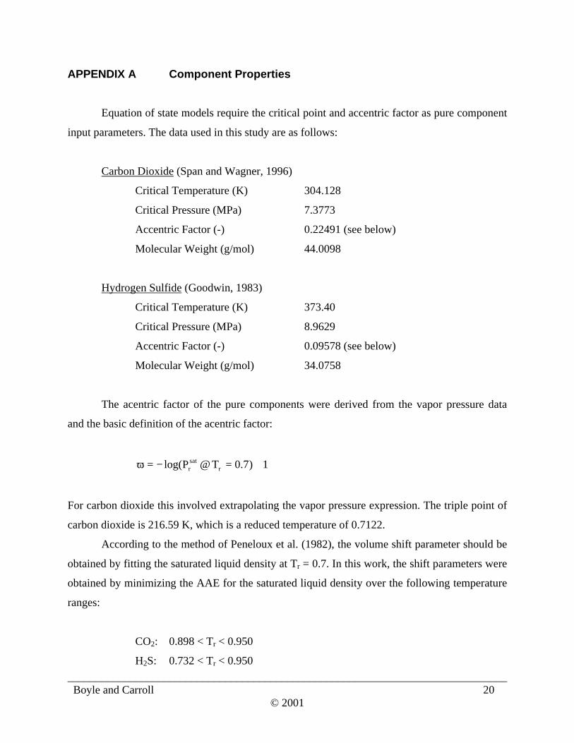
APPENDIX A Component Properties

Equation of state models require the critical point and accentric factor as pure component

input parameters. The data used in this study are as follows:

Carbon Dioxide (Span and Wagner, 1996)

Critical Temperature (K) 304.128

Critical Pressure (MPa) 7.3773

Accentric Factor (-) 0.22491 (see below)

Molecular Weight (g/mol) 44.0098

Hydrogen Sulfide (Goodwin, 1983)

Critical Temperature (K) 373.40

Critical Pressure (MPa) 8.9629

Accentric Factor (-) 0.09578 (see below)

Molecular Weight (g/mol) 34.0758

The acentric factor of the pure components were derived from the vapor pressure data

and the basic definition of the acentric factor:

1)7.0T@Plog( rsatr +=−=ω

For carbon dioxide this involved extrapolating the vapor pressure expression. The triple point of

carbon dioxide is 216.59 K, which is a reduced temperature of 0.7122.

According to the method of Peneloux et al. (1982), the volume shift parameter should be

obtained by fitting the saturated liquid density at Tr = 0.7. In this work, the shift parameters were

obtained by minimizing the AAE for the saturated liquid density over the following temperature

ranges:

CO2: 0.898 < Tr < 0.950

H2S: 0.732 < Tr < 0.950


© 2001

The lower reduced temperature corresponds to 0°C, the lowest temperature of interest in this

study. For the SRK the following Peneloux-type volume shift parameters were used:

/molcm6650.8c 3CO2

−=

/molcm3826.3c 3H2

−=S

And for the PR equation the following parameters were used here:

/molcm7493.1c 3CO2

−=

/molcm2176.2c 3H2

+=S

For the Mathias-type correction to the PR equation the s parameter was obtained by

fitting the saturated liquid density at Tr = 0.7 (or nearly so). The vc values were obtained by

minimizing the AAE for the range of saturated liquid given above.

/molcm585.1s 3CO2

= (from matching the saturated liquid density

at Tr = 0.712, CO2 triple point)

/molcm998.2s 3H2

=S (from matching the saturated liquid density at Tr = 0.7097)

/molcm001.96v 3COc, 2

= (2% larger than the experimental critical volume)

/molcm490.100v 3Hc, 2

=S (2.5% larger than the experimental critical volume)

For the PT equation the following parameters were used in this study:

CO2: F = 0.707727 cζ = 0.309

H2S: F = 0.583165 cζ = 0.320


© 2001

which were taken from the paper of Patel and Teja (1982). The above values result in smaller

errors in the density than the values from the generalized correlations.

Mixtures

Equation of state models require binary interaction parameters for multi-component input

parameters. The binary interaction coefficients for H2S – CO2 used in this study are as follows:

0.0989 for SRK

0.0974 for PR

0.0975 for PT

The values for the SRK and PR equations are from Knapp et al. (1982). These values are those

given in the popular book by Reid et al. (1987). The interaction parameter for the PT equation is

an estimate based on the values for the other two equations.


© 2001

APPENDIX B Equation of State Summary

The material that follows provides the details of the three equations of state used in this

study. Only the equations are provided, no discussion or derivation.

Soave-Redlich-Kwong Equation of State

)bv(v

a

bv

TRP

+⋅−

−⋅

=

0)BA(Z)BBA(ZZ 223 =⋅−⋅−−+−

where:

ci

2ci

ci P

)TR(42748.0a

⋅⋅=

icii aa α⋅=

)T1(m1 5.0rii

5.0i −⋅+=α

2iii 176.0574.148.0m ω⋅−ω⋅+=

∑∑ −⋅⋅=N

iij

5.0jij

N

ji )k1()aa(xxa

2)TR(

PaA

⋅⋅

=

ci

cii P

TR08664.0b

⋅⋅=

∑ ⋅=N

iii bxb

TR

PbB

⋅⋅

=


© 2001

Peng-Robinson Equation of State

)bv(b)bv(v

a

bv

TRP

−⋅++⋅−

−⋅

=

0)BBBA(Z)B3B2A(Z)B1(Z 32223 =−−⋅−⋅⋅−⋅−+⋅−−

where

ci

2ci

ci P

)TR(457235.0a

⋅⋅=

icii aa α⋅=

)T1(m1 5.0rii

5.0i −⋅+=α

2iii ù0.26992ù1.542260.37464m ⋅−⋅+=

∑∑ −⋅⋅=N

iij

5.0jij

N

ji )k1()aa(xxa

2)TR(

PaA

⋅⋅

=

ci

cii P

TR077796.0b

⋅⋅=

∑ ⋅=N

iii bxb

TR

PbB

⋅⋅

=


© 2001

The Patel-Teja Equation of State

)bv(c)bv(v

a

bv

TRP

−⋅++⋅−

−⋅

=

0)BACBCB(Z)ACBBCB2(Z)1C(Z 2223 =⋅−⋅+⋅+⋅+−−−⋅⋅−+⋅−+

where

ci

2ci

aci P

)TR(a

⋅⋅Ω=

icii aa α⋅=

)T1(F1 5.0ri

5.0i −⋅+=α

∑∑ −⋅⋅=N

iij

5.0jij

N

ji )k1()aa(xxa

2)TR(

PaA

⋅⋅

=

ci

cibi P

)TR(b

⋅⋅Ω=

∑ ⋅=N

iii bxb

TR

PbB

⋅⋅

=

ci

cici P

)TR(c

⋅⋅Ω=

∑ ⋅=N

iii cxc

TR

PcC

⋅⋅

=


© 2001

3c

2bbc

2ca 3)21(33 ζ⋅−Ω+Ω⋅ζ⋅−⋅+ζ⋅=Ω

and Ωb is the smallest real root of the following equation:

03)32( 3cb

2c

2bc

3b =ζ−Ω⋅ζ⋅+Ω⋅ζ⋅−+Ω

cc 31 ζ⋅−=Ω

The parameters F and cζ can be optimized from a set of data or they can be obtained from the

following generalized equations:

2295937.030982.1452413.0F ω⋅−ω⋅+=

2c 0211947.0076799.0329032.0 ω⋅−ω⋅−=ζ

____________________________________________________________________________________________________________ Boyle and Carroll 27

© 2001

Figure 1. Density Errors Associated with the Original SRK Equation for Carbon Dioxide

0.0

5.0

10.0

15.0

20.0

25.0

30.0

0.85 0.90 0.95 1.00 1.05 1.10 1.15 1.20 1.25 1.30 1.35 1.40 1.45 1.50

Tr

% E

rror

Pr = 0.678 (liquid)

Pr = 0.678 (vapor)

Pr = 0.949 (liquid)

Pr = 0.949 (vapour)

Pr = 1.356

Pr = 2.711

Pr = 4.067

Pr sat (liquid)

Pr sat (vapor)

critical point


© 2001

Figure 2. Density Errors Associated with the SRK-Peneloux Equation for Carbon Dioxide

-20.0

-15.0

-10.0

-5.0

0.0

5.0

10.0

15.0

20.0

0.85 0.90 0.95 1.00 1.05 1.10 1.15 1.20 1.25 1.30 1.35 1.40 1.45 1.50

Tr

% E

rror

Pr = 0.678 (liquid)

Pr = 0.678 (vapor)

Pr = 0.949 (liquid)

Pr = 0.949 (vapour)

Pr = 1.356

Pr = 2.711

Pr = 4.067

Pr sat (liquid)

Pr sat (vapor)

critical point


© 2001

Figure 3. Density Errors Associated with the Original PR Equation for Carbon Dioxide

-10.0

-5.0

0.0

5.0

10.0

15.0

20.0

0.85 0.90 0.95 1.00 1.05 1.10 1.15 1.20 1.25 1.30 1.35 1.40 1.45 1.50

Tr

% E

rror

Pr = 0.678 (liquid)

Pr = 0.678 (vapor)

Pr = 0.949 (liquid)

Pr = 0.949 (vapour)

Pr = 1.356

Pr = 2.711

Pr = 4.067

Pr sat (liquid)

Pr sat (vapor)

critical point


© 2001

Figure 4. Density Errors Associated with the PR-Peneloux Equation for Carbon Dioxide

-15.0

-10.0

-5.0

0.0

5.0

10.0

15.0

20.0

0.85 0.90 0.95 1.00 1.05 1.10 1.15 1.20 1.25 1.30 1.35 1.40 1.45 1.50

Tr

% E

rror

Pr = 0.678 (liquid)

Pr = 0.678 (vapor)

Pr = 0.949 (liquid)

Pr = 0.949 (vapour)

Pr = 1.356

Pr = 2.711

Pr = 4.067

Pr sat (liquid)

Pr sat (vapor)

critical point


© 2001

Figure 5. Density Errors Associated with the PR-Mathias Equation for Carbon Dioxide

-10.0

-5.0

0.0

5.0

10.0

0.85 0.90 0.95 1.00 1.05 1.10 1.15 1.20 1.25 1.30 1.35 1.40 1.45 1.50

Tr

% E

rror

Pr = 0.678 (liquid)

Pr = 0.678 (vapor)

Pr = 0.949 (liquid)

Pr = 0.949 (vapour)

Pr = 1.356

Pr = 2.711

Pr = 4.067

Pr sat (liquid)

Pr sat (vapor)

critical point


© 2001

Figure 6. Density Errors Associated with the Original PT Equation for Carbon Dioxide

-5.0

0.0

5.0

10.0

15.0

20.0

0.85 0.90 0.95 1.00 1.05 1.10 1.15 1.20 1.25 1.30 1.35 1.40 1.45 1.50

Tr

% E

rror

Pr = 0.678 (liquid)

Pr = 0.678 (vapor)

Pr = 0.949 (liquid)

Pr = 0.949 (vapour)

Pr = 1.356

Pr = 2.711

Pr = 4.067

Pr sat (liquid)

Pr sat (vapor)

critical point


© 2001

Figure 7. Density Errors Associated with the Original SRK Equation for Hydrogen Sulfide

-5.0

0.0

5.0

10.0

15.0

20.0

25.0

0.70 0.75 0.80 0.85 0.90 0.95 1.00 1.05 1.10 1.15 1.20 1.25

Tr

% E

rror

Pr = 0.558 (liquid)

Pr = 0.558 (vapor)

Pr = 0.893 (liquid)

Pr = 0.893 (vapour)

Pr = 1.674

Pr = 2.231

Pr = 3.347

Pr sat (liquid)

Pr sat (vapor)

critical point


© 2001

Figure 8. Density Errors Associated with the SRK-Peneloux Equation for Hydrogen Sulfide

-10.0

-5.0

0.0

5.0

10.0

15.0

20.0

0.70 0.75 0.80 0.85 0.90 0.95 1.00 1.05 1.10 1.15 1.20 1.25

Tr

% E

rror

Pr = 0.558 (liquid)

Pr = 0.558 (vapor)

Pr = 0.893 (liquid)

Pr = 0.893 (vapour)

Pr = 1.674

Pr = 2.231

Pr = 3.347

Pr sat (liquid)

Pr sat (vapor)

critical point


© 2001

Figure 9. Density Errors Associated with the Original PR Equation for Hydrogen Sulfide

-10.0

-5.0

0.0

5.0

10.0

15.0

0.70 0.75 0.80 0.85 0.90 0.95 1.00 1.05 1.10 1.15 1.20 1.25

Tr

% E

rror

Pr = 0.558 (liquid)

Pr = 0.558 (vapor)

Pr = 0.893 (liquid)

Pr = 0.893 (vapour)

Pr = 1.674

Pr = 2.231

Pr = 3.347

Pr sat (liquid)

Pr sat (vapor)

critical point


© 2001

Figure 10. Density Errors Associated with the PR-Peneloux Equation for Hydrogen Sulfide

-10.0

-5.0

0.0

5.0

10.0

15.0

20.0

0.70 0.75 0.80 0.85 0.90 0.95 1.00 1.05 1.10 1.15 1.20 1.25

Tr

% E

rror

Pr = 0.558 (liquid)

Pr = 0.558 (vapor)

Pr = 0.893 (liquid)

Pr = 0.893 (vapour)

Pr = 1.674

Pr = 2.231

Pr = 3.347

Pr sat (liquid)

Pr sat (vapor)

critical point


© 2001

Figure 11. Density Errors Associated with the PR-Mathias Equation for Hydrogen Sulfide

-10.0

-5.0

0.0

5.0

10.0

0.70 0.75 0.80 0.85 0.90 0.95 1.00 1.05 1.10 1.15 1.20 1.25

Tr

% E

rror

Pr = 0.558 (liquid)

Pr = 0.558 (vapor)

Pr = 0.893 (liquid)

Pr = 0.893 (vapour)

Pr = 1.674

Pr = 2.231

Pr = 3.347

Pr sat (liquid)

Pr sat (vapor)

critical point


© 2001

Figure 12. Density Errors Associated with the Original PT Equation for Hydrogen Sulfide

-5.0

0.0

5.0

10.0

15.0

20.0

0.70 0.75 0.80 0.85 0.90 0.95 1.00 1.05 1.10 1.15 1.20 1.25

Tr

% E

rror

Pr = 0.558 (liquid)

Pr = 0.558 (vapor)

Pr = 0.893 (liquid)

Pr = 0.893 (vapour)

Pr = 1.674

Pr = 2.231

Pr = 3.347

Pr sat (liquid)

Pr sat (vapor)

critical point


© 2001

Figure 13. Density Errors Associated with Each Equation for the 90.45 mol% CarbonDioxide - 9.55 mol% Hydrogen Sulfide Mixture at Tr = 1.140 (Supercritical Region)

-10.0

-8.0

-6.0

-4.0

-2.0

0.0

2.0

4.0

0.00 0.50 1.00 1.50 2.00 2.50 3.00

Pr

% E

rror

SRK

SRK-Peneloux

PR

PR-Peneloux

PR-Mathias

PT


© 2001

Figure 14. Density Errors Associated with Each Equation for the 70.67 mol% CarbonDioxide - 29.33 mol% Hydrogen Sulfide Mixture at Tr = 1.266 (Supercritical Region)

-4.0

-2.0

0.0

2.0

4.0

6.0

0.00 0.50 1.00 1.50 2.00 2.50 3.00

Pr

% E

rror

SRK

SRK-Peneloux

PR

PR-Peneloux

PR-Mathias

PT


© 2001

Figure 15. Density Errors Associated with Each Equation for the 50.01 mol% CarbonDioxide - 49.99 mol% Hydrogen Sulfide Mixture at Tr = 0.912 (Liquid Region)

-8.0

-4.0

0.0

4.0

8.0

12.0

16.0

0.60 0.80 1.00 1.20 1.40 1.60 1.80 2.00 2.20 2.40 2.60

Pr

% E

rror

SRK

SRK-Peneloux

PR

PR-Peneloux

PR-Mathias

PT

CALCULATION OF ACID GAS DENSITY IN THE VAPOR, … · CALCULATION OF ACID GAS DENSITY IN THE VAPOR,...

Documents

Transcript of CALCULATION OF ACID GAS DENSITY IN THE VAPOR, … · CALCULATION OF ACID GAS DENSITY IN THE VAPOR,...