Calculation for axial-radial-roller bearings

The software calculates the stiffness, the load distribution and the life of axial-radial-roller bearings.

The geometry of parts is defined by horizontal and vertical lines; several parts can be defined. The

parts can be connected axially or radially by bearings. A bolted joint and loads on surfaces or point

loads can be considered.

The deformation of parts is calculated by a nonlinear FEA, while the coupling to the rollers is done

analytically according ISO/TS 16281. Bolts are modeled using beam elements.

A first calculation step is done to evaluate the bolt pretension without further loads. Further

calculation steps are then done with loading.

General usage The software can be called with several file names on the commend line. All calculations are run

sequentially and the report is generated without showing a user interface. Example:

„MesysAxRaRBC.exe file1.xml file2.xml“

For larger models the calculation time can be up to an hour. Therefore the following approach is

recommended: Choose ‘Only preprocessing’ and build the model interactively. Save the model and

run the calculation using the command line. Afterwards the results can be loaded into the program

to evaluate the results.

If several calculations have to be run the software can be called with several file names. These

calculations are done sequentially. The FEA is using up to two processor cores. If more cores are

available the program can be started in parallel to run multiple calculations if the amount of memory

is sufficient.

The number of processor cores used in FEA can be changed by changing following entry in mesys.ini:

[axrarbc]

numberofthreads=2

Using more than two threads will lead only to small improvements.

Inputs The input data is provided on several input pages which are described on the following pages. The

input data is for the following geometry:

General

General

Number of parts

The bearing can be build using several parts. In usual cases two parts are used. There is no restriction

on the number of parts.

Number of bearings

The number of radial, axial and cross roller bearings can be defined here. In usual cases one radial

and two axial bearings are needed.

Maximum angle for mesh

For the meshing in circumferential direction a maximum angle can be defined. Using a value of zero

the angle results from number of bolts and rollers. The angle can only be reduced but not be

increased.

A large angle can lead to increased stiffness of the parts. To estimate the influence of the angle soma

calculations for comparison can be made.

Number of bolted joints

One or more rings of bolts can optionally be considered.

Consider load spectrum

A load spectrum can be considered. If a calculation of series is active only multiple speeds can be

defined. Without calculation of series also different loads can be defined per load spectrum element.

Only preprocessing

If this option is activated only the model is created but no FEA is performed on running the

calculation.

Allow general geometry input

If this option is not set the geometry is defined by horizontal and vertical lines only. This allowed to

enter one number only per geometry line.

If the option is activated all values for the geometry coordinated have to be defined, but a general

polygon is permitted as geometry. A meshing algorithm is used then that will lead to less elements

then with horizontal and vertical lines only.

Number of surface loads

The number of loads acting on surfaces can be defined using this input value.

Reliability of rolling bearings

The bearing reliability is 90% as default. The input is used for the calculation of life modification

factor a1.

The reliability is set for all bearings to the same value.

Series calculation

A series of load cases can be calculated by multiplying the load with a factor.

The load factor for the first calculation is the ‘start factor’ for the last calculation the ‘end factor’ is

used. A given number of steps is calculated in between. For the results a selection is available for the

load step shown in graphics.

Lubrication

For the calculation of modified life the definition of the lubrication is needed. The lubricant viscosity

is calculated for the lubricant temperature using the reference values at 40°C and 100°C.

The selection ‘consider lubrication’ defines if the modified life Lnmrh and the data for lubrication is

shown in the report. For small rotation speed there will be effective lubrication the aISO factor

approaches 0.1.

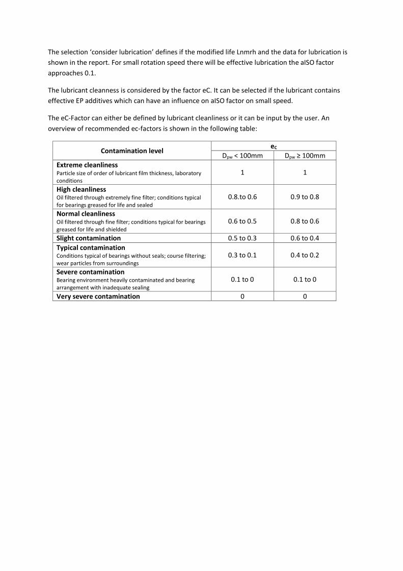
The lubricant cleanness is considered by the factor eC. It can be selected if the lubricant contains

effective EP additives which can have an influence on aISO factor on small speed.

The eC-Factor can either be defined by lubricant cleanliness or it can be input by the user. An

overview of recommended ec-factors is shown in the following table:

Contamination level eC

Dpw < 100mm Dpw ≥ 100mm

Extreme cleanliness Particle size of order of lubricant film thickness, laboratory conditions

1 1

High cleanliness Oil filtered through extremely fine filter; conditions typical for bearings greased for life and sealed

0.8.to 0.6 0.9 to 0.8

Normal cleanliness Oil filtered through fine filter; conditions typical for bearings greased for life and shielded

0.6 to 0.5 0.8 to 0.6

Slight contamination 0.5 to 0.3 0.6 to 0.4

Typical contamination Conditions typical of bearings without seals; course filtering; wear particles from surroundings

0.3 to 0.1 0.4 to 0.2

Severe contamination Bearing environment heavily contaminated and bearing arrangement with inadequate sealing

0.1 to 0 0.1 to 0

Very severe contamination 0 0

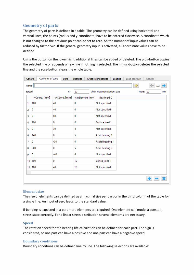
Geometry of parts The geometry of parts is defined in a table. The geometry can be defined using horizontal and

vertical lines; the points (radius and y-coordinate) have to be entered clockwise. A coordinate which

is not changed to the previous point can be set to zero. So the number of input values can be

reduced by factor two. If the general geometry input is activated, all coordinate values have to be

defined.

Using the button on the lower right additional lines can be added or deleted. The plus-button copies

the selected line or appends a new line if nothing is selected. The minus-button deletes the selected

line and the ross-button clears the whole table.

Element size

The size of elements can be defined as a maximal size per part or in the third column of the table for

a single line. An input of zero leads to the standard value.

If bending is expected in a part more elements are required. One element can model a constant

stress state correctly. For a linear stress distribution several elements are necessary.

Speed

The rotation speed for the bearing life calculation can be defined for each part. The sign is

considered, so one part can have a positive and one part can have a negative speed.

Boundary conditions

Boundary conditions can be defined line by line. The following selections are available:

Radial fixed: All nodes for this surface are fixed radially

Axial fixed: All nodes for this surface are fixed axially

Radial and axial fixed: All nodes for this surface are fixed radially and axially

Bolted joint: The head of the bolts is on this plane

Radial bearing: A radial bearing is connected to this plane

Axial bearing: An axial bearing is connected to this plane. This input is used for axial

positioning.

Cross roller bearing: A cross roller bearing is connected to this surface.

Surface load: A load is applied to this surface

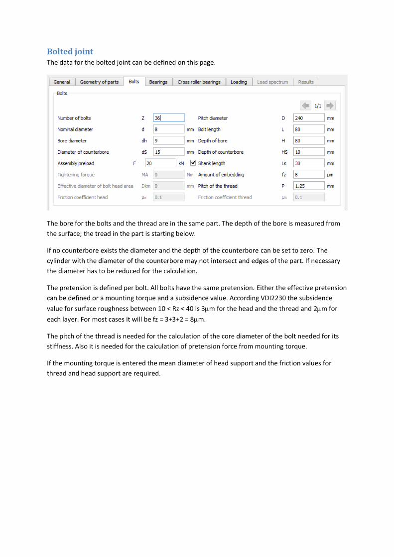
Bolted joint The data for the bolted joint can be defined on this page.

The bore for the bolts and the thread are in the same part. The depth of the bore is measured from

the surface; the tread in the part is starting below.

If no counterbore exists the diameter and the depth of the counterbore can be set to zero. The

cylinder with the diameter of the counterbore may not intersect and edges of the part. If necessary

the diameter has to be reduced for the calculation.

The pretension is defined per bolt. All bolts have the same pretension. Either the effective pretension

can be defined or a mounting torque and a subsidence value. According VDI2230 the subsidence

value for surface roughness between 10 < Rz < 40 is 3m for the head and the thread and 2m for

each layer. For most cases it will be fz = 3+3+2 = 8m.

The pitch of the thread is needed for the calculation of the core diameter of the bolt needed for its

stiffness. Also it is needed for the calculation of pretension force from mounting torque.

If the mounting torque is entered the mean diameter of head support and the friction values for

thread and head support are required.

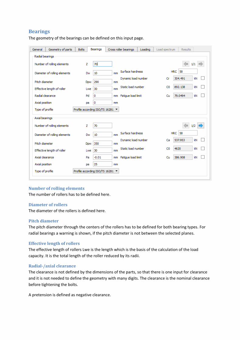
Bearings The geometry of the bearings can be defined on this input page.

Number of rolling elements

The number of rollers has to be defined here.

Diameter of rollers

The diameter of the rollers is defined here.

Pitch diameter

The pitch diameter through the centers of the rollers has to be defined for both bearing types. For

radial bearings a warning is shown, if the pitch diameter is not between the selected planes.

Effective length of rollers

The effective length of rollers Lwe is the length which is the basis of the calculation of the load

capacity. It is the total length of the roller reduced by its radii.

Radial-/axial clearance

The clearance is not defined by the dimensions of the parts, so that there is one input for clearance

and it is not needed to define the geometry with many digits. The clearance is the nominal clearance

before tightening the bolts.

A pretension is defined as negative clearance.

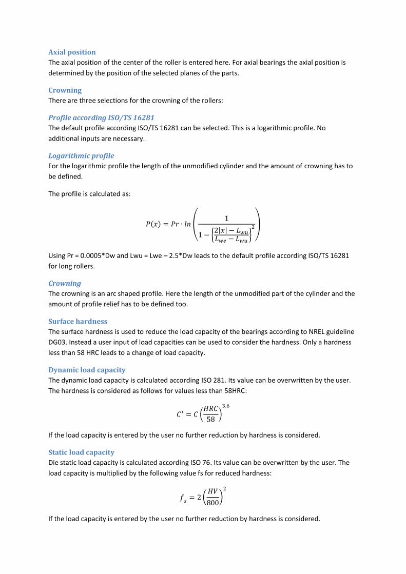
Axial position

The axial position of the center of the roller is entered here. For axial bearings the axial position is

determined by the position of the selected planes of the parts.

Crowning

There are three selections for the crowning of the rollers:

Profile according ISO/TS 16281

The default profile according ISO/TS 16281 can be selected. This is a logarithmic profile. No

additional inputs are necessary.

Logarithmic profile

For the logarithmic profile the length of the unmodified cylinder and the amount of crowning has to

be defined.

The profile is calculated as:

𝑃(𝑥) = 𝑃𝑟 ∙ 𝑙𝑛

(

1

1 − {2|𝑥| − 𝐿𝑤𝑢𝐿𝑤𝑒 − 𝐿𝑤𝑢

}2

)

Using Pr = 0.0005*Dw and Lwu = Lwe – 2.5*Dw leads to the default profile according ISO/TS 16281

for long rollers.

Crowning

The crowning is an arc shaped profile. Here the length of the unmodified part of the cylinder and the

amount of profile relief has to be defined too.

Surface hardness

The surface hardness is used to reduce the load capacity of the bearings according to NREL guideline

DG03. Instead a user input of load capacities can be used to consider the hardness. Only a hardness

less than 58 HRC leads to a change of load capacity.

Dynamic load capacity

The dynamic load capacity is calculated according ISO 281. Its value can be overwritten by the user.

The hardness is considered as follows for values less than 58HRC:

𝐶′ = 𝐶 (𝐻𝑅𝐶

58)3.6

If the load capacity is entered by the user no further reduction by hardness is considered.

Static load capacity

Die static load capacity is calculated according ISO 76. Its value can be overwritten by the user. The

load capacity is multiplied by the following value fs for reduced hardness:

𝑓𝑠= 2 (

𝐻𝑉

800)2

If the load capacity is entered by the user no further reduction by hardness is considered.

Fatigue load

The fatigue load is calculated according ISO 281 appendix B.3.3.3. The value can be overwritten by

the user.

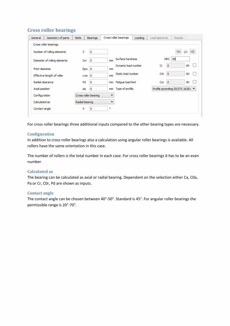
Cross roller bearings

For cross roller bearings three additional inputs compared to the other bearing types are necessary.

Configuration

In addition to cross roller bearings also a calculation using angular roller bearings is available. All

rollers have the same orientation in this case.

The number of rollers is the total number in each case. For cross roller bearings it has to be an even

number.

Calculated as

The bearing can be calculated as axial or radial bearing. Dependent on the selection either Ca, C0a,

Pa or Cr, C0r, Pd are shown as inputs.

Contact angle

The contact angle can be chosen between 40°-50°. Standard is 45°. For angular roller bearings the

permissible range is 20°-70°.

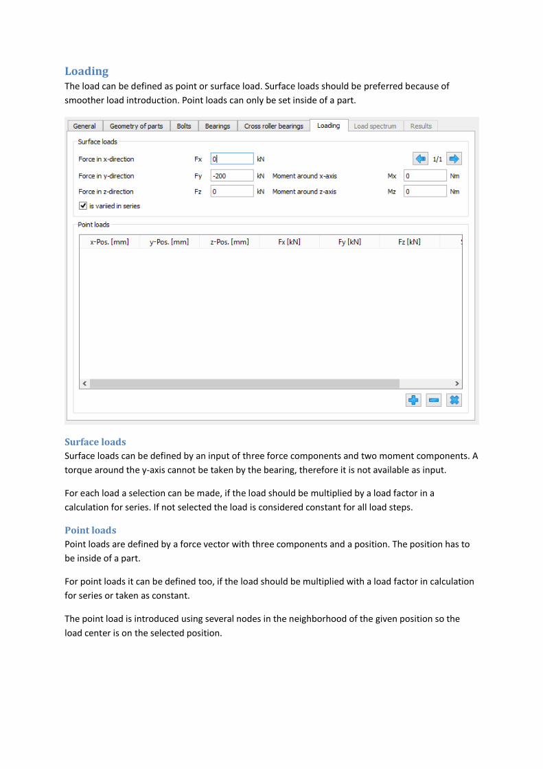
Loading The load can be defined as point or surface load. Surface loads should be preferred because of

smoother load introduction. Point loads can only be set inside of a part.

Surface loads

Surface loads can be defined by an input of three force components and two moment components. A

torque around the y-axis cannot be taken by the bearing, therefore it is not available as input.

For each load a selection can be made, if the load should be multiplied by a load factor in a

calculation for series. If not selected the load is considered constant for all load steps.

Point loads

Point loads are defined by a force vector with three components and a position. The position has to

be inside of a part.

For point loads it can be defined too, if the load should be multiplied with a load factor in calculation

for series or taken as constant.

The point load is introduced using several nodes in the neighborhood of the given position so the

load center is on the selected position.

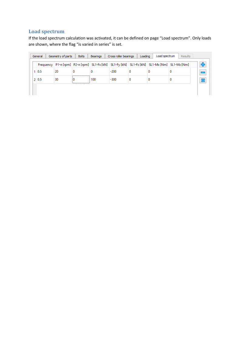
Load spectrum If the load spectrum calculation was activated, it can be defined on page “Load spectrum”. Only loads

are shown, where the flag “is varied in series” is set.

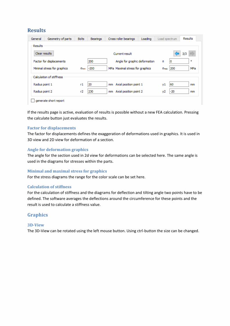
Results

If the results page is active, evaluation of results is possible without a new FEA calculation. Pressing

the calculate button just evaluates the results.

Factor for displacements

The factor for displacements defines the exaggeration of deformations used in graphics. It is used in

3D view and 2D view for deformation of a section.

Angle for deformation graphics

The angle for the section used in 2d view for deformations can be selected here. The same angle is

used in the diagrams for stresses within the parts.

Minimal and maximal stress for graphics

For the stress diagrams the range for the color scale can be set here.

Calculation of stiffness

For the calculation of stiffness and the diagrams for deflection and tilting angle two points have to be

defined. The software averages the deflections around the circumference for these points and the

result is used to calculate a stiffness value.

Graphics

3D-View

The 3D-View can be rotated using the left mouse button. Using ctrl-button the size can be changed.

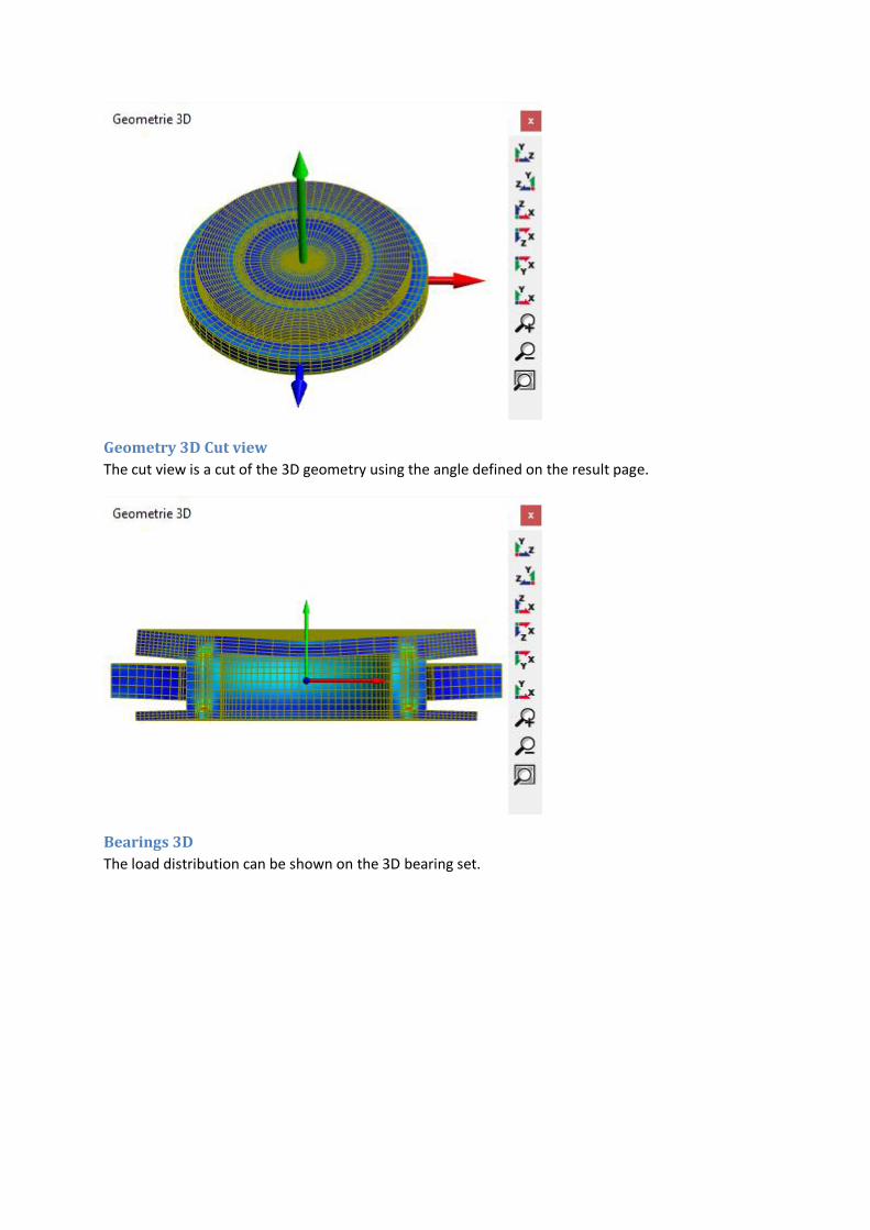
Geometry 3D Cut view

The cut view is a cut of the 3D geometry using the angle defined on the result page.

Bearings 3D

The load distribution can be shown on the 3D bearing set.

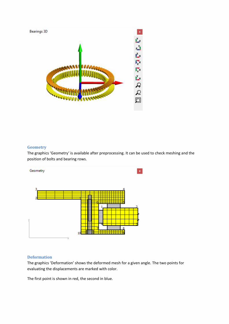
Geometry

The graphics ‘Geometry‘ is available after preprocessing. It can be used to check meshing and the

position of bolts and bearing rows.

Deformation

The graphics ‘Deformation’ shows the deformed mesh for a given angle. The two points for

evaluating the displacements are marked with color.

The first point is shown in red, the second in blue.

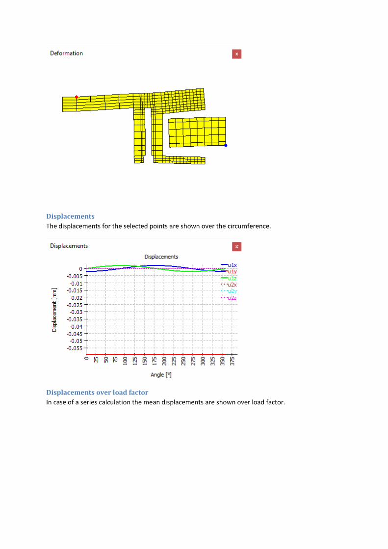
Displacements

The displacements for the selected points are shown over the circumference.

Displacements over load factor

In case of a series calculation the mean displacements are shown over load factor.

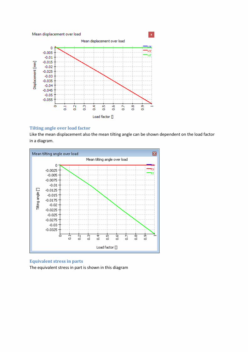
Tilting angle over load factor

Like the mean displacement also the mean tilting angle can be shown dependent on the load factor

in a diagram.

Equivalent stress in parts

The equivalent stress in part is shown in this diagram

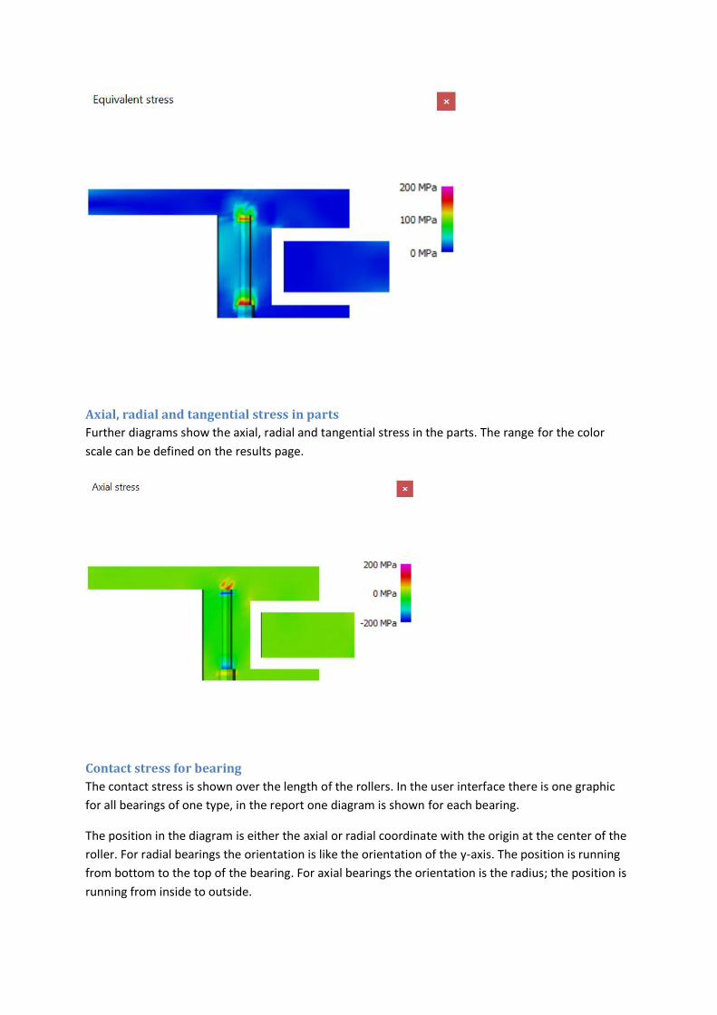
Axial, radial and tangential stress in parts

Further diagrams show the axial, radial and tangential stress in the parts. The range for the color

scale can be defined on the results page.

Contact stress for bearing

The contact stress is shown over the length of the rollers. In the user interface there is one graphic

for all bearings of one type, in the report one diagram is shown for each bearing.

The position in the diagram is either the axial or radial coordinate with the origin at the center of the

roller. For radial bearings the orientation is like the orientation of the y-axis. The position is running

from bottom to the top of the bearing. For axial bearings the orientation is the radius; the position is

running from inside to outside.

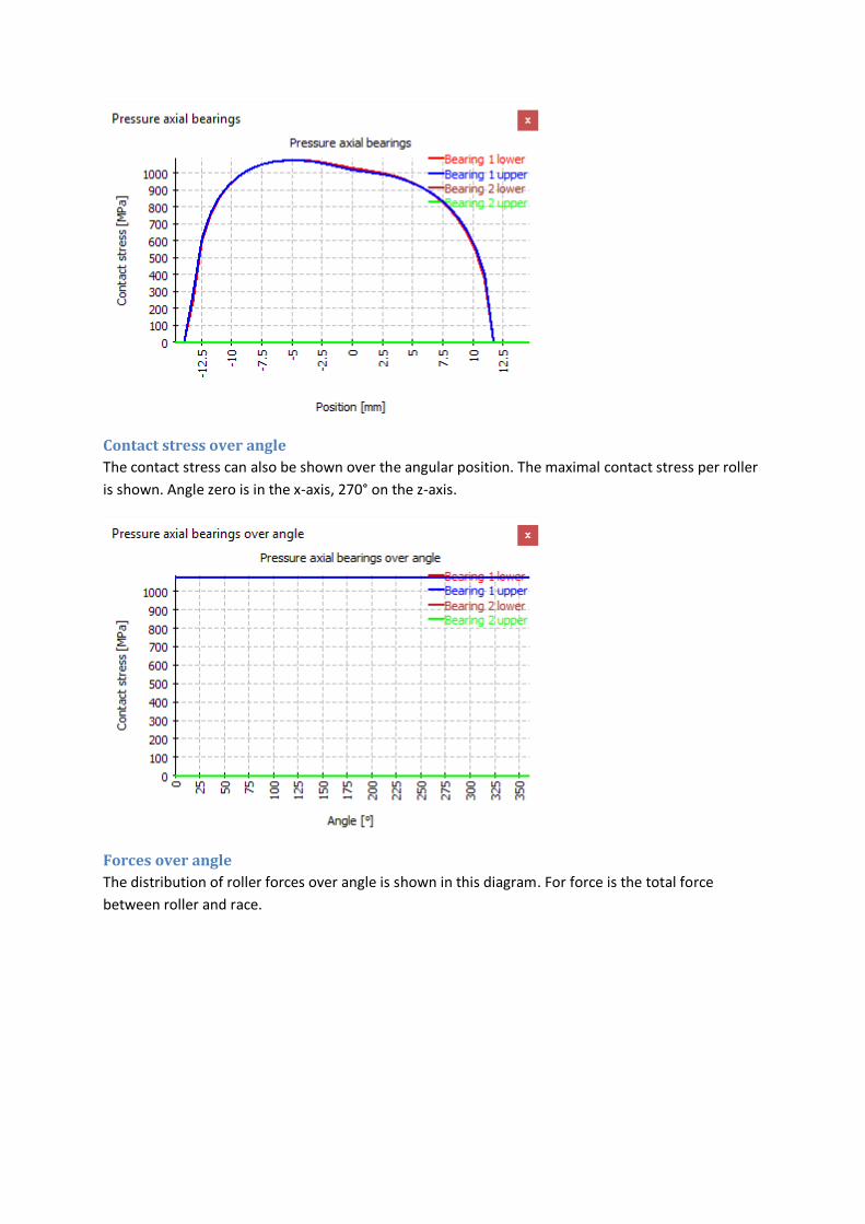
Contact stress over angle

The contact stress can also be shown over the angular position. The maximal contact stress per roller

is shown. Angle zero is in the x-axis, 270° on the z-axis.

Forces over angle

The distribution of roller forces over angle is shown in this diagram. For force is the total force

between roller and race.

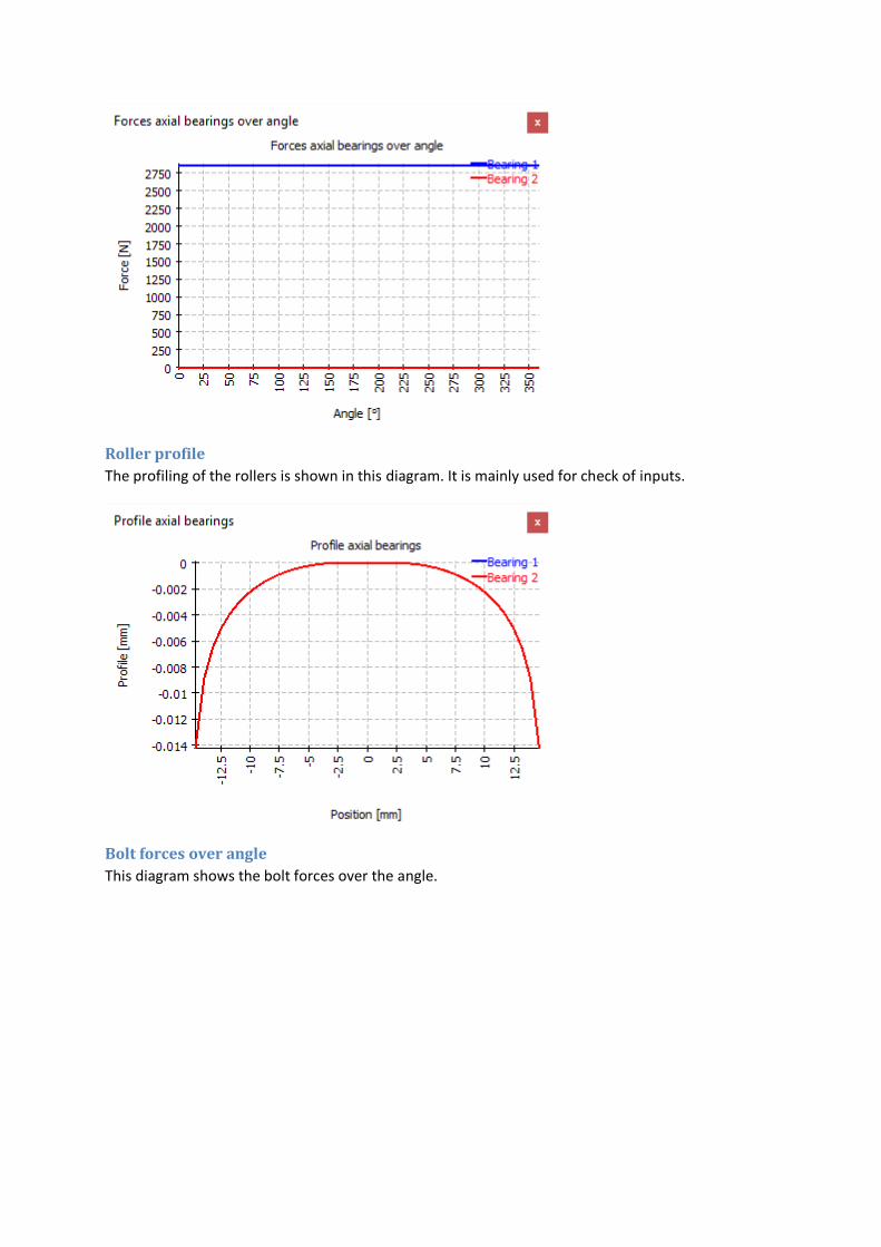
Roller profile

The profiling of the rollers is shown in this diagram. It is mainly used for check of inputs.

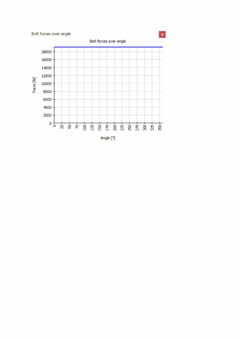
Bolt forces over angle

This diagram shows the bolt forces over the angle.