Calabi-Yau Geometry and Higher Genus Mirror Symmetry

A dissertation presented

by

Si Li

to

The Department of Mathematics

in partial fulfillment of the requirementsfor the degree of

Doctor of Philosophyin the subject of

Mathematics

Harvard UniversityCambridge, Massachusetts

May 2011

© 2011 – Si LiAll rights reserved.

iii

Dissertation Advisor: Professor Shing-Tung Yau Si Li

Calabi-Yau Geometry and Higher Genus Mirror Symmetry

Abstract

We study closed string mirror symmetry on compact Calabi-Yau manifolds at higher

genus. String theory predicts the existence of two sets of geometric invariants, from the

A-model and the B-model on Calabi-Yau manifolds, each indexed by a non-negative inte-

ger called genus. The A-model has been mathematically established at all genera by the

Gromov-Witten theory, but little is known in mathematics for B-model beyond genus zero.

We develop a mathematical theory of higher genus B-model from perturbative quantiza-

tion techniques of gauge theory. The relevant gauge theory is the Kodaira-Spencer gauge

theory, which is originally discovered by Bershadsky-Cecotti-Ooguri-Vafa as the closed

string field theory of B-twisted topological string on Calabi-Yau three-folds. We generalize

this to Calabi-Yau manifolds of arbitrary dimensions including also gravitational descen-

dants, which we call BCOV theory. We give the geometric description of the perturbative

quantization of BCOV theory in terms of deformation-obstruction theory. The vanishing

of the relevant obstruction classes will enable us to construct the higher genus B-model.

We carry out this construction on the elliptic curve and establish the corresponding higher

genus B-model. Furthermore, we show that the B-model invariants constructed from BCOV

theory on the elliptic curve can be identified with descendant Gromov-Witten invariants

on the mirror elliptic curve. This gives the first compact Calabi-Yau example where mirror

symmetry can be established at all genera.

iv

Contents

Acknowledgements vi

1. Introduction 1

1.1. The A-model and Gromov-Witten theory 3

1.2. The B-model and BCOV theory 5

1.3. Main results 8

2. Classical Geometry of Calabi-Yau Moduli Space 10

2.1. Polyvector fields 10

2.2. Deformation theory of Calabi-Yau manifolds 16

2.3. Special geometry and tt∗ Equations 20

2.4. Yukawa coupling and prepotential 26

2.5. Kodaira-Spencer gauge theory 30

3. Perturbative Quantization of Gauge Theory 33

3.1. Feynman Diagrams 33

3.2. Batalin-Vilkovisky geometry 36

3.3. Effective field theory and renormalization 47

3.4. Gauge theory and quantum master equation 54

3.5. Feynman graph integral for holomorphic theory on C 65

4. Quantum Geometry of Calabi-Yau Manifolds 72

4.1. Classical BCOV theory 72

4.2. Quantization and higher genus B-model 77

5. Quantization of BCOV theory on elliptic curves 84

5.1. Deformation-obstruction complex 84

5.2. Uniqueness of the quantization 89

5.3. Existence of the quantization 94

5.4. Holomorphicity 99

5.5. Local renormalization group flow 113

5.6. Virasoro equations 116

6. Higher genus mirror symmetry on elliptic curves 121

6.1. BCOV propagator on elliptic curves 123

v

6.2. Boson-Fermion correspondence 128

6.3. Gromov-Witten invariants on elliptic curves 135

6.4. τ →∞ limit 143

6.5. Proof of mirror symmetry 157

Appendix A. L∞ algebra 159

A.1. L∞ structure 159

A.2. Maurer-Cartan equation 163

A.3. Homotopy 165

A.4. Deformation functor 166

Appendix B. D-modules and Jets 167

B.1. D-module 167

B.2. Jet bundles 169

B.3. Local functionals 172

References 173

vi

Acknowledgements

Foremost, I would like to express my deep and sincere gratitude to my thesis advisor

Professor Shing-Tung Yau. I have benefited incredibly in the past five years from his broad

and thoughtful view in mathematics and physics, his generosity in sharing his ideas, and

his invaluable support and encouragement in my research projects.

I am deeply grateful to Professor Kevin Costello, who had kindly explained to me his

work on renormalization theory. Part of the thesis grew out of a joint project with him and

was carried out while visiting the math department of Northwestern University. I thank

for their hospitality. I wish to pay special thanks to Professor Cumrun Vafa for many

stimulating discussions and his wonderful lectures in string theory, which has always been

an important origin of my curiosity throughout my research. I also want to pay sincere

thanks to Professor Kefeng Liu and Professor Sen Hu for their help and support in the past

years both in my career and in my life.

There are many people who have helped me financially for my graduate study. I want

to express my deep thanks to Mr. Sze-Lim Li, who had supported my first year life in

the United States. Without him I wouldn’t even have this wonderful chance to come to

Harvard. I also want to thank Mr. Raphael Salem. The fellowship at Harvard under his

name has helped me survive in the academic year 2008-2009.

I sincerely appreciate the useful conversations at Harvard with Chien-Hao Liu, Valentino

Tosatti, Chen-Yu Chi, Yu-Shen Lin, at Brandeis with Bong H. Lian, at Northwestern with

Yuan Shen, and at various workshops and online MSN with Huai-Liang Chang. I would

also like to thank the participants of Yau’s student seminar, who have helped to realize

my ignorance in diverse branches of mathematics. This includes in addition: Wenxuan Lu,

Ming-Tao Chuan, PoNing Chen, Ruifang Song, Aleksandar Subotic, Yi Li, Jie Zhou, Yih

Sung, Li-Sheng Tseng, Baosen Wu and Peng Zhang. Special thank goes to Chen-Yu Chi,

who has always been available to discuss math anytime during the 24 hours a day, 7 days

a week. Moreover, without his generous and constant provision of chocolates and desserts

for the alcove around our offices, I wouldn’t gain so much weight in the past few years.

vii

Among my graduate friends at Harvard math department, I would like to thank specially

to Le Anh Vinh and Henry Shin. Without them, I would not be so poor after we invented

our strange bill system to pay so many enjoyable dinners.

In addition, I appreciate the work of many secretaries at Harvard math department, in-

cluding Maureen Armstrong, Susan Gilbert, Robbie Miller, Nancy Miller and Irene Minder.

I’m also grateful to Robin Gottlieb, Janet Chen and Jameel Al-Aidroos for their helps on

various aspects of my teaching at Harvard.

There are many other friends at Harvard outside math department contributing to my

meaningful life here. My special gratitude is due to my roommates, Nan Sun and Qu Zhang,

together with whom we have maintained a three-year “gelivable” life style, the “Mellen

System” named by our friends. In addition, I thank Nan Sun for his constant bothering

of interesting math problems in engineering that I’ve never been able to solve, which has

helped me to understand the power and the limitation of math tools in real world problems.

I thank Qu Zhang for our long discussion of a project on modelling the high proportion of

fixed nucleotide substitutions in orangutan, which has never really started, and from which

I have learned so many interesting aspects of population genetics and coalescent theory.

Lastly and most importantly, I wish to thank my family. I’m deeply indebted to my

parents for their selfless love and enormous care since I was born. Without their support, I

could not have gone this far. I want to tell them that I miss you so much. I owe my loving

thanks to my wife Xuejing. She has sacrificed so much due to my personal choice on career,

my working style on research, and our long-distance relationship in the past seven years. I

thank wholeheartedly for her tremendous love and exclusive understanding, without which

this work would not be possible. I would like to take this opportunity to say that I love

you.

1

1. Introduction

Mirror symmetry originated from string theory as a duality between superconformal field

theories (SCFT). The natural geometric background involved is the Calabi-Yau manifold,

and SCFTs can be realized from twisting the so-called σ-models on Calabi-Yau manifolds in

two different ways [Wit88, Wit92]: the A-model and the B-model. The physics statement

of mirror symmetry says that the A-model on a Calabi-Yau manifold X is equivalent to the

B-model on a different Calabi-Yau manifold X, which is called the mirror.

The mathematical interests on mirror symmetry started from the work [CdlOGP91],

where a remarkable mathematical prediction was extracted from the physics statement

of mirror symmetry: the counting of rational curves on the Quintic 3-fold is equivalent

to the period integrals on the mirror Quintic 3-fold. Motivated by this example, people

have conjectured that such phenomenon holds for general mirror Calabi-Yau manifolds.

The counting of rational curves is refered to as the genus 0 A-model, which has now been

mathematically established [RT94, LT98] as Gromov-Witten theory. The period integral

is related to the variation of Hodge structure, and this is refered to as the genus 0 B-

model. Mirror conjecture at genus 0 has been proved by Givental [Giv98] and Lian-Liu-Yau

[LLY97] for a large class of Calabi-Yau manifolds inside toric varieties. In the last twenty

years, mirror symmetry has lead to numerous deep connections between various branches

of mathematics and has been making a huge influence on both mathematics and physics.

The fundamental mathematical question is to understand mirror symmetry at higher

genus. In the A-model, the Gromov-Witten theory has been established for curves of

arbitrary genus, and the problem of counting higher genus curves on Calabi-Yau manifolds

has a solid mathematical foundation. However, little is known for the higher genus B-model.

One mathematical approach to the higher genus B-model given by Kevin Costello [Cos09]

is categorical, from the viewpoint of Kontsevich’s homological mirror symmetry [Kon95b].

The B-model partition function is proposed through the Calabi-Yau A-infinity category

of coherent sheaves and a classification of certain 2-dimensional topological field theories.

Unfortunately, the computation from categorical aspects is extremely difficult that only

results for zero dimensional space, i.e. a point, have been obtained.

2

On the other hand, in the breakthrough work [BCOV94] on topological string theory,

Bershadsky-Cecotti-Ooguri-Vafa proposed a closed string field theory interpretation of the

B-model, and suggested that the B-model partition function could be constructed from

a quantum field theory, which is called the Kodaira-Spencer gauge theory of gravity in

[BCOV94]. The solution space of the classical equations of motion in Kodaira-Spencer

gauge theory describes the moduli space of deformations of complex structures on the

underlying Calabi-Yau manifold, from which we can recover the well-known geometry of

the genus 0 B-model. We will call this quantum field theory as BCOV theory. Following

this philosophy, a non-trivial prediction has been made in [BCOV94], which says that the

genus one partition function in the B-model on Calabi-Yau three-fold is given by certain

holomorphic Ray-Singer torsion and it could be identified with the genus one Gromov-

Witten invariants on the mirror Calabi-Yau three-fold. This is recently confirmed by Zinger

in [Zin93].

The main purpose of this thesis is to understand BCOV theory from the mathematical

point of view. In physics, the main difficulty in understanding a quantum gauge theory

lies in the appearance of singularities and gauge anomalies arising from the path integral

quantization, and this is where the celebrated idea of renormalization comes into playing a

significant role. One mathematical approach for perturbative renormalization of quantum

field theories based on Wilson’s effective action philosophy is developed by Kevin Costello

in [Cos11]. We will develop the general framework of constructing higher genus B-model

from BCOV theory using the techniques of perturbative renormalization theory. We carry

out the construction in details for the case of one-dimensional Calabi-Yaus, i.e., elliptic

curves, and prove that the corresponding B-model partition function is identical to the

A-model partition function constructed from Gromov-Witten theory on the mirror elliptic

curves. This is the first example of compact Calabi-Yau manifolds where mirror symmetry

is established at all genera. The thesis is based mainly on the work [CL, Li].

We will give a brief description of the main results in this introduction. In section 1.1,

we collect some basics facts on Gromov-Witten theory and the A-model. In section 1.2, we

describe the geometry of B-model and the BCOV theory. In section 1.3, we state the main

result for the higher genus mirror symmetry on the elliptic curve.

3

1.1. The A-model and Gromov-Witten theory. Let X be a smooth projective al-

gebraic variety with complexified Kahler form ωX , where ReωX is a Kahler form, and

ImωX ∈ H2(X,R)/H2(X,Z). The Gromov-Witten theory on X concerns the moduli space

Mg,n,β(X)

parametrizing Kontsevich’s stable maps [Kon95a] f from connected, genus g, nodal curve

C to X, with n distinct smooth marked points, such that

f∗[C] = β ∈ H2(X,Z)

This moduli space is equipped with evaluation maps

evi : Mg,n,β(X) → X

[f, (C; p1, · · · , pn)] → evi ([f, (C; p1, · · · , pn)]) = f(pi)

The cotangent line to the ith marked point is a line bundle on Mg,n,β(X), whose first Chern

class will be denoted by ψi ∈ H2(Mg,n,β(X)

). The Gromov-Witten invariants of X are

defined by

〈−〉 : SymnC (H∗(X)[[t]]) → C⟨

tk1α1, · · · , tknαn⟩Xg,n,β

=

∫[Mg,n,β(X)]

virψk1

1 ev∗1α1 · · ·ψknn ev∗nαn

where[Mg,n,β(X)

]viris the virtual fundamental class [LT98, BF97] of Mg,n,β(X), which is

a homology class of dimension

(3− dimX) (2g − 2) + 2

∫βc1(X) + 2n(1.1)

Definition 1.1. X is a Calabi-Yau variety if its anti-canonical bundle is trivial.

From now on we will focus on Calabi-Yau varieties. From (1.1), we see that in the

Calabi-Yau case, the dimension of the virtual fundamental class doesn’t depend on β, since

c1(X) = 0.

4

Definition 1.2. The genus g A-model partition function FAg,n,X;q[−] with n inputs is defined

to be the multi-linear map

FAg,n,X;q : Symn

C (H∗(X,C)[[t]]) → C

FAg,n,X;q

[tk1α1, · · · , tknαn

]=

∑β∈H2(X,Z)

q∫β ωX

⟨tk1α1, · · · , tknαn

⟩Xg,n,β

where q is a formal variable.

The A-model partition function satisfies the following basic properties

(1) Degree Axiom. FAg,n,X;q

[tk1α1, · · · , tknαn

]is non-zero only for

n∑i=1

(degαi + 2ki) = (2g − 2) (3− dimX) + 2n

Moreover, we have the Hodge decomposition Hn(X,C) =⊕

p+q=nHp,q. If we define

the Hodge weight of tkα ∈ tk Hp,q by HW(tkα) = k+p−1, then the reality condition

implies the Hodge weight condition

n∑i=1

HW(αi) = (g − 1) (3− dimX)

(2) String equation. FAg,n,X;q satisfies the string equation

FAg,n+1,X;q

[1, tk1α1, · · · , tknαn

]=

n∑i=1

FAg,n,X;q

[tk1α1, · · · , tki−1αi, · · · tknαn

](3) Dilaton equation. FA

g,n,X;q satisfies the dilaton equation

FAg,n,X;q

[t, tk1α1, · · · , tknαn

]= (2g − 2 + n)FA

g,n,X;q

[tk1α1, · · · , tknαn

]The parameter q can be viewed as the Kahler moduli. Since the Gromov-Witten invariants

are invariant under complex deformations, FAg,n,X;q only depends on the Kahler moduli, but

not on the complex moduli of X. This is the special property characterizing the A-model.

A special role is played by Calabi-Yau 3-folds where the original mirror symmetry is

established. In the case of dimension 3,

dim[Mg,n,β(X)

]vir= 2n

5

Definition 1.3. The Yukawa coupling in the A-model is defined to be the genus 0 3-point

correlation function

H∗(X)⊗3 → C

α⊗ β ⊗ γ → FA0,3,X;q [α, β, γ]

If β = 0, we know that the Gromov-Witten invariants are reduced to the classical inter-

section product

〈α, β, γ〉0,3,β=0 =

∫Xα ∧ β ∧ γ

Therefore, the A-model Yukawa coupling

FA0,3,X;q [α, β, γ] =

∫Xα ∧ β ∧ γ +

∑β 6=0

q∫β ωX

∫[M0,3,β(X)]

virev∗1α ∧ ev∗2β ∧ ev∗3γ

can be viewed as a quantum deformation of the classical intersection product. Moreover,

it gives a q-deformation of the classical ring structure of H∗(X,C), which is called the

quantum cohomology ring.

1.2. The B-model and BCOV theory. The geometry of B-model concerns the moduli

space of complex structures of Calabi-Yau manifolds. Let Xτ be a Calabi-Yau 3-fold with

nowhere vanishing holomorphic volume form ΩXτ. Let TXτ be the holomorphic tangent

bundle. Here τ parametrizes the complex structures of X.

Definition 1.4. The B-model Yukawa coupling is defined to be

H∗(Xτ ,∧∗TXτ )⊗3 → C

µ1 ⊗ µ2 ⊗ µ3 → FB0,3,Xτ

[µ1, µ2, µ3] =

∫Xτ

(µ1 ∧ µ2 ∧ µ3 ` ΩXτ

)∧ ΩX

where ` is the natural contraction between tensors in ∧∗TX and ∧∗T ∗X

.

Generally speaking, string theory predicts that we should also have the B-model corre-

lation functions

FBg,n,Xτ

: SymnC(H∗(Xτ ,∧∗TXτ )[[t]]

)→ C

6

However, little is known for genus g > 0 and the inclusion of gravitational descendants t is

even more mysterious.

Motivated by the physics idea of [BCOV94], we will approach the B-model correlation

functions from the renormalization of BCOV theory using the techniques developed by

[Cos11]. Let ΩXτbe a fixed nowhere vanishing holomorphic volume form. The existence of

ΩXτis guaranteed by the Calabi-Yau condition. Let

EXτ = PV∗,∗Xτ

[[t]]

be the space of fields of BCOV theory, where PV∗,∗Xτ

is the space of polyvector fields, see

(2.1). We define the classical BCOV action as a functional on EXτ by

SBCOV =∑n≥3

SBCOVn

where

SBCOVn : Sym(E ⊗nXτ

)→ C

tk1µ1 ⊗ · · · ⊗ tknµn →∫M0,n

ψk11 · · ·ψ

knn

∫Xτ

(µ1 · · ·µn ` ΩXτ

)∧ ΩXτ

where∫M0,n

ψk11 · · ·ψknn =

(n−3

k1,··· ,kn)

is the ψ-class integration. Let

Q = ∂ − t∂ : EXτ → EXτ

be the differential, and we refer to (4.1) and the corresponding section for the detailed

explanation. Q induces a derivation on the space of functionals on EXτ , which we still

denote by Q. Let −.− be the Poisson bracket on local functionals defined by definition

4.4. Then SBCOV satisfies the following classical master equation (see Lemma 4.6)

QSBCOV +1

2

SBCOV , SBCOV

= 0(1.2)

The physics meaning of classical master equation is that SBCOV is endowed with a gauge

symmetry. SBCOV generalizes the original Kodaira-Spencer gauge action on Calabi-Yau 3-

folds [BCOV94] to arbitrary dimensions, and remarkably, it also includes the gravitational

descendants t.

7

Let KL be the Heat kernel of the operator e−L∆ and ∂KL be the smooth kernel of

∂e−L∆, for L > 0. We define the regularized propagator PLε by the smooth kernel of the

operator −∫ Lε ∂∗∂e−u∆du, for ε, L > 0. Both ∂KL and PLε define operators on the space

of functionals∂

∂PLε, ∆L =

∂

∂ (∂KL)

via contraction, see Definition 3.23 and Definition 4.7.

We would like to construct the quantization of the BCOV theory on Xτ , which is given

by a family of functionals on EXτ valued in C[[~]] parametrized by L > 0

F[L] =∑g≥0

~gFg[L]

which satisfies the renormalization group flow equation

eF[L]/~ = e~ ∂

∂PLε eF[ε]/~, ∀ε, L > 0

the classical limit condition: F[L] has a small L asymptotic expansion in terms of local

functionals as L→ 0 and

limL→0

F0[L] = SBCOV

the quantum master equation

(Q+ ~∆L) eF[L]/~ = 0, ∀L > 0

and certain other properties such as the string equations and dilaton equations in this

context. All of these will be discussed in details in section 4.

Once we have constructed the quantization F[L], we can let L→∞. Since limL→∞

KL be-

comes the Harmonic projection, we see that limL→∞

∂KL = 0. The quantum master equation

at L =∞ says

QF[∞] = 0

This implies that F[∞] induces a well-defined functional on the Q-cohomology of EXτ . We

will write

F[∞] =∑g≥0

~gFBg,Xτ

8

Using the isomorphism (see Lemma 4.10)

H∗(EXτ , Q) ∼= H∗(Xτ ,∧∗TXτ )[[t]]

and decomposing FBg,X

into number of inputs, we can define the genus g B-model correlation

functions by

FBg,n,X

: SymnC(H∗(Xτ ,∧∗TXτ )[[t]]

)→ C

Therefore the problem of constructing higher genus B-model is reduced to the construc-

tion of the quantization F[L]. The general formalism of [Cos11] tells us that the quan-

tization is controlled by certain L∞ algebraic structure on the space of local functionals

on EXτ . There’s an obstruction class for constructing Fg[L] at each genus g > 0, and it’s

natural is conjecture that all the obstruction classes vanish for BCOV theory. For X being

one-dimensional, i.e., the elliptic curve, we will show that this is indeed the case.

To establish mirror symmetry at higher genus, we need to compare the A-model corre-

lation function FAg,n,X;q with the B-model correlation function FB

g,n,Xτ. In general, FB

g,n,Xτ

doesn’t depend holomorphically on τ , and there’s so-called holomorphic anomalies discov-

ered by [BCOV94]. It’s predicted by [BCOV94] that we should be able to make sense

of the limit limτ→∞

FBg,n,Xτ

around the large complex limit of Xτ . The higher genus mirror

conjecture can be stated as the identification of

FAg,n,X;q ←→ limτ→∞

FBg,n,Xτ

under certain identification of cohomology classes

H∗(X,∧∗T ∗X)←→ H∗(Xτ ,∧∗TXτ )

and the mirror map between Kahler moduli and complex moduli

q ←→ τ

1.3. Main results. Let Xτ = Eτ be the elliptic curve C/ (Z⊕ Zτ), where τ lies in the

upper-half plane viewed as the complex moduli of E.

9

Theorem 1.5 ([CL]). There exists a unique quantization FEτ [L] of BCOV theory on Eτ

satisfying the dilaton equation. Morever, FEτ [L] satisfies the Virasoro equations.

Section 5 is devoted to explain and prove this theorem.

Since we know that the A-model Gromov-Witten invariants on the elliptic curve also

satisfies the Virasoro equations [OP06b], the proof of mirror symmetry can be reduced to

the so-called stationary sectors [OP06a]. More precisely, let E the dual elliptic curve of E

and ω ∈ H2(E,Z) be the dual class of a point. The stationary sector of Gromov-Witten

invariants are defined for descendants of ω

⟨tk1ω, · · · , tknω

⟩g,d,E

=

∫[Mg,n(E,d)]vir

n∏i=1

ψkii ev∗i (ω)

On the other hand, we let ω ∈ H1(Eτ , TEτ ) be the class such that Tr(ω) = 1.

Theorem 1.6 ([Li]). For any genus g ≥ 0, n > 0, and non-negative integers k1, · · · , kn,

(1) FEτg [∞][tk1ω, · · · , tknω] is an almost holomorphic modular form of weight

n∑i=1

(ki + 2) = 2g − 2 + 2n

It follows that the limit limτ→∞

FEτg [∞][tk1ω, · · · , tknω] makes sense and is a quasi-

modular form of the same weight.

(2) The higher genus mirror symmetry holds on elliptic curves in the following sense

∑d≥0

qd⟨tk1ω, · · · , tknω

⟩g,d,E

= limτ→∞

FEτg [∞][tk1ω, · · · , tknω]

under the identification q = exp(2πiτ).

Section 6 is denoted to prove this theorem.

10

2. Classical Geometry of Calabi-Yau Moduli Space

In this section, we discuss some basics on the classical geometry of the moduli space of

Calabi-Yau manifolds, with the purpose of motivating the Kodaira-Spencer gauge theory.

We will also set up our notations that will be used throughout this thesis.

2.1. Polyvector fields. In this subsection we describe the Batalin-Vilkovisky structure of

polyvector fields on the Calabi-Yau manifolds.

2.1.1. DGA structure. Let X be a compact Calabi-Yau manifold of dimension d. Let

PV∗,∗X =⊕

0≤i,j≤dPVi,j

X PVi,jX = A0,j(X,∧iTX)(2.1)

denote the space of polyvector fields on X. Here TX is the holomorphic tangent bundle

of X, and A0,j(X,∧iTX) is the space of smooth (0, j)-forms valued in ∧iTX . PV∗,∗X is a

differential bi-graded commutative algebra; the differential is the operator

∂ : PVi,j(X)→ PVi,j+1(X).

and the algebra structure arises from wedging polyvector fields. The degree of elements

of PVi,jX is i + j. Explicitly, let zi be local holomorphic coordinates on X. Let I =

i1, i2, · · · , ik be an ordered subset of 1, 2, · · · , d, with |I| = k. We will use the following

notations

dzI = dzi1 ∧ dzi2 ∧ · · · ∧ dzik , ∂

∂zI=

∂

∂zi1∧ ∂

∂zi2∧ · · · ∧ ∂

∂zik

and similarly for dzI and ∂∂zI

. Given α ∈ PVi,jX , β ∈ PVk,l

X , we write in local coordinates

α =∑

|I|=i,|J |=j

αIJdzJ ⊗ ∂

∂zI, β =

∑|K|=k,|L|=l

βKL dzL ⊗ ∂

∂zK

then

∂α =∑

|I|=i,|J |=j

∂αIJ ∧ dzJ ⊗ ∂

∂zI(2.2)

11

and the product structure is given by

αβ ≡ α ∧ β =∑

|I|=i,|J |=j|K|=k,|L|=l

(−1)ilαIJβKL dz

J ∧ dzL ⊗ ∂

∂zI∧ ∂

∂zK(2.3)

The graded-commutativity says that

αβ = (−1)|α||β|βα(2.4)

where |α|, |β| denote the degree of α, β respectively.

2.1.2. Batalin-Vilkovisky structure. Calabi-Yau condition implies that there exists a nowhere

vanishing holomorphic volume form

ΩX ∈ Ωd,0(X)

which is unique up to a multiplication by a constant. Let us fix a choice of ΩX . It induces

an isomorphism between the space of polyvector fields and differential forms

PVi,jX

`ΩX∼= Ad−i,jX(2.5)

α → α ` ΩX(2.6)

where ` is the contraction map, which is defined in local coordinates on the basis

∂

∂zI` dzJ =

(−1)|I|(|I|−1)/2dzK if dzJ = dzI ∧ dzK , I ∩K = ∅

0 otherwise

(2.7)

The holomorphic de Rham differential ∂ on differential forms defines an operator on

polyvector fields via the above isomorphism, which we still denote by ∂

∂ : PVi,jX → PVi−1,j

X

i.e.

(∂α) ` ΩX ≡ ∂(α ` ΩX), α ∈ PVi,jX(2.8)

Obviously, the definition of ∂ doesn’t depend on the choice of ΩX .

12

Given α ∈ PV∗,∗X , the multiplication

α∧ : PV∗,∗X → PV∗,∗X

defines an operator acting on polyvector fields which has the same degree as α.

Lemma 2.1. For any α, β, γ ∈ PV∗,∗X ,

[[[∂, α], β], γ] = 0

viewed as an operator acting on PV∗,∗X . Here [·, ·] is the graded commutator.

Proof. This follows from direct calculation in local coordinates.

It follows from the lemma that the operator [[∂, α], β] is equivalent to multiplying by a

polyvector fields, which defines the bracket

α, β = [[∂, α], β] ∈ PV∗,∗X(2.9)

The bracket used here differs from the Schouten-Nijenhuis bracket by a sign. More

precisely, if we let , sn denote the Schouten-Nijenhuis bracket, then

α, βsn = −(−1)|α|α, β(2.10)

In particular, if both α, β ∈ PV1,0X , then α, β is just the ordinary Lie-bracket on vector

fields.

Lemma 2.2. The following properties hold

(1) Graded symmetry

α, β = (−1)deg(α) deg(β)β, α

(2) Leibniz relation

α, β ∧ γ = α, β ∧ γ + (−1)|β||γ|α, γ ∧ β

13

(3) Graded Jacobi Identity

α, β, γ = −(−1)|α|α, β, γ − (−1)(|α|+1)|β|β, α, γ

(4) Batalin-Vilkoviski identity (Todorov-Tian’s lemma)

∂(α ∧ β) = (∂α) ∧ β + (−1)αα ∧ ∂β + α, β

Proof. Since [α, β] = 0, it follows from the Jacobi identity that

[[∂, α], β] = [∂, [α, β]]− (−1)|α|[α, [∂, β]] = (−1)|α||β|[[∂, β], α]

This proves (1).

α, β ∧ γ = [[∂, α], β ∧ γ]

= −(−1)|α|[α, [∂, β ∧ γ]]

= −(−1)|α|[α, [∂, β]γ + (−1)|β||γ|[∂, γ]β]

= −(−1)|α|[α, [∂, β]]γ − (−1)|α|+|β||γ|[α, [∂, γ]]β

= α, β ∧ γ + (−1)|β||γ|α, γ ∧ β

This proves (2).

α, β, γ = [[∂, [[∂, α], β]], γ]

= (−1)|α|+|β|[[[∂, α], β], [∂, γ]]

= (−1)|α|+|β|[[∂, α], [β, [∂, γ]]]− (−1)|α||β|+|α|[β, [[∂, α], [∂, γ]]]

= (−1)|α|+|β|[[∂, α], [β, [∂, γ]]]− (−1)|α||β|+|α|[β, [∂, [α, [∂, γ]]]]

= −(−1)|α|α, β, γ − (−1)(|α|+1)|β|β, α, γ

where on the fourth line we have used the fact that [∂, [∂, ·]] = 0. This proves (3).

To prove (4), we identify ∂(α ∧ β) with the action of the operator [∂, α ∧ β] on 1 since

∂(1) = 0. Therefore

∂(α ∧ β) = [∂, α ∧ β] · 1

14

= [∂, α]β · 1 + (−1)|α|α ∧ ∂β

= [[∂, α], β] + (−1)|β|(|α|+1)β ∧ ∂α+ (−1)|α|α ∧ ∂β

= (∂α) ∧ β + (−1)|α|α ∧ ∂β + α, β

Remark 2.3. The Batalin-Vilkovisky identity has the natural generalization

∂(α1 ∧ · · · ∧ αn) =∑i

±(∂αi)α1 ∧ · · · αi · · · ∧ αn +∑i 6=j±αi, αjα1 ∧ · · · αi · · · αj · · · ∧ αn

where the signs are given by permuting the α’s. The proof is similar.

Definition 2.4. A Batalin-Vilkovisky algebra (BV algebra) is given by the tuple

(A, ·,∆, , ) where

(1) A is a graded vector space.

(2) · : A⊗A → A is associative and graded commutative.

(3) ∆ : A → A is an odd differential of degree (-1).

(4) , : A⊗A → A is a bilinear operation such that for all α, β, γ ∈ A

∆(α · β) = (∆α) · β + (−1)|α|α ·∆β + (−1)|α|α, β

α, β · γ = α, β · γ + (−1)(|α|+1)|β|β · α, γ

Corollary 2.5. The tuple(PV∗,∗X ,∧, ∂,−, sn

)is a BV algebra. Here , sn is the Schouten-

Nijenhuis bracket (see (2.10)).

2.1.3. The trace map. Define a map

Tr : PV∗,∗X → C

by

Tr(α) =

∫X(α ` ΩX) ∧ ΩX if α ∈ PVd,d

X

0 if α 6∈ PVd,dX

(2.11)

15

The pairing

PVi,j(X)⊗ PVd−i,d−j(X) → C

α⊗ β → Tr(αβ)

is non-degenerate, i.e., it has no kernel.

Lemma 2.6. The operator ∂ is skew self-adjoint for the pairing Tr(αβ), and the operator

∂ is self-adjoint for this pairing.

Proof. The fact that ∂ is skew self adjoint follows immediately from the fact that ∂ is a

derivation for the algebra structure on PV∗,∗X . For ∂, First we know that

Tr ((∂α)β) =

∫X

((∂α)β ` ΩX) ∧ ΩX

= ±∫X

(∂α ` Ω) ∧ (β ` ΩX)

= ±∫X

(α ` Ω) ∧ (∂β ` ΩX)

= ±∫X

(α ∧ ∂β ` Ω) ∧ ΩX

= ±Tr (α∂β)

for some sign ±. To determine this sign, we choose local holomorphic coordinates z1, · · · , zd

such that ΩX = dz1 ∧ · · · ∧ dzd, then it’s easy to see that

∂ =∑i

∂

∂zi∂

∂(∂zi)

where ∂∂(∂zi )

is the odd derivation generated by

∂

∂(∂zi)∂zj = δji

Therefore the sign can be determined by

Tr ((∂α)β) = −∑i

Tr

((∂

∂(∂zi)α

)∂

∂ziβ

)= (−1)|α|Tr (α∂β)

16

2.2. Deformation theory of Calabi-Yau manifolds.

2.2.1. Local deformation of complex structures. Let X be a compact Calabi-Yau manifold

of dimension d with a fixed Kahler metric. We assume that H0(X,TX) = 0. The complex

structure of X is equivalent to the decomposition of the complexified cotangent bundles

Ω1X ⊗R C = Ω1,0

X ⊕ Ω0,1X

into types (1, 0) and (0, 1) with additional integrability conditions. We consider a nearby

deformation of the complex structure, which can be viewed as deforming the above decom-

position into new types of (1, 0) and (0, 1) forms. This can be described as follows: let

µ ∈ PV1,1X be a smooth polyvector field, and z1, · · · , zd are local holomorphic coordinates

on X such that locally

µ =d∑i=1

µijdzj ⊗ ∂

∂zi

If ‖µ‖ is sufficiently small (‖·‖ is the norm with respect to the fixed metric), then we obtain

a new almost complex structure Jµ by requiring that the new (1, 0)-form is spanned locally

by

θi = dzi + µ ` dzi, 1 ≤ i ≤ d(2.12)

The integrability condition says that dθi is of type (2, 0) + (1, 1) in the new decomposition,

which is equivalent to

∂µ+1

2µ, µ = 0(2.13)

Let DefX be the local universal deformation space of X, which is a germ of the Te-

ichmuller space of X at the given complex structure of X. DefX represents the following

deformation functor

DefX : Artin local C-algebra → sets

17

such that for a given Artin local C-algebra A with maximal ideal mA,

DefX(A) =

µ ∈ PV1,1

X ⊗mA

∣∣∣ ∂µ+1

2µ, µ = 0

/ ∼

The equivalence relation is given by the gauge action of PV1,0⊗mA on PV1,1⊗mA

µ→ eadα(µ) +Id−eadα

adα∂α

for α ∈ PV1,0⊗mA, µ ∈ PV1,1⊗mA. Here adα is the adjoint action α, ·. This equivalence

can be viewed as generated by diffeomorphisms. From the general theory of deformation

of complex structures, the tangent space of the germ DefX is given by

DefX(C[ε]/ε2) = H1(X,TX)

and H2(X,TX) serves as an obstruction space for the deformation functor DefX .

In the case of Calabi-Yau manifolds, the deformation functor DefX is unobstructed and

DefX is the germ of a smooth manifold. To see this, let

µ1 ∈ H0,1

∂(X,TX)

be a harmonic element with respect to the Kahler metric. µ1 represents a tangent vector

of DefX . We need to prove the existence of

µt ∈ PV1,1X ⊗C[[t]]

such that

∂µt +1

2µt, µt = 0, µt ≡ tµ1 mod t2

Then an argument of Kuranishi shows that the formal power series is convergent given t

sufficiently small. It follows that every first order deformation can be realized, i.e., DefX

is unobstructed.

We follow the approach of Todorov [Tod89] to construct µt. By Todorov-Tian’s lemma

as in Lemma 2.2, the bracket , preserves the subspace ker ∂ ⊂ PV∗,∗X

, : ker ∂ ⊗ ker ∂ → im ∂ ⊂ ker ∂(2.14)

18

If we write

µt =∑i≥1

tiµi

then µi, i ≥ 2, can be solved recursive by imposing the following equation

µt − tµ1 = −1

2∂∗Gµt, µt(2.15)

Here G = 1∆ is the Green operator with respect to the Kahler metric. Explicitly,

µi = −1

2

i−1∑k=1

∂∗Gµk, µi−k, ∀i ≥ 2

We show that such constructed µ indeed solves Eqn (2.13) and satisfies

∂∗µt = ∂µt = 0

First, observe that the recursive relation and (2.14) implies that

µi ∈ im ∂, ∀i ≥ 2

Apply ∂ to (2.15), we find

∂µt = −1

2∂∂∗Gµt, µt = −1

2µt, µt+

1

2∂∗G∂µt, µt

where we have used the fact that µt, µt ∈ im ∂ has no harmonic part. Therefore

∂µt, µt = 2∂µt, µt = −µt, µt, µt+ ∂∗G∂µt, µt, µt

Jacobi Identity implies that µt, µt, µt = 0, hence

∂µt, µt = ∂∗G∂µt, µt, µt

This recursive relation and the initial condition ∂µ1, µ1 = 0 implies that

∂µt, µt = 0

which in turn implies

∂µt = −1

2µt, µt

19

The deformation of the holomorphic volume form can be also described by this solution.

Let Ω0 be the holomorphic volume form on the undeformed X. Consider

Ωt = eµt ` Ω0(2.16)

From (2.12), we see that Ωt is of type (d,0) in the new complex structure given by µt. Since

dΩt =(∂eµt + ∂eµt

)` Ω0 =

(∂µt + ∂µt +

1

2µt, µt

)eµt ` Ω0 = 0

where we have used the BV identity in Remark 2.3. It follows that Ωt is in fact holomorphic

in the new complex structure.

If folows from the unobstructedness of DefX that we can choose a linear coordinate

ti of H1(X,TX) as local coordinates of DefX . This is called the canonical coordinate,

which is unique up to linear transformations. The corresponding holomorphic family of top

holomorphic forms (2.16) is called the canonical family of holomorphic volume forms.

2.2.2. Extended deformation space and the Formality Theorem. The smoothness theorem

for Calabi-Yau manifolds is extended in [BK98] to a bigger deformation space whose tangent

space includes all ⊕i,j

Hi(X,∧jTX)

We give a brief discussion here for the purpose of later discussion on the higher genus

B-model.

The deformation functor DefX is the restriction of the moduli functor associated with

the DGLA (PV1,∗

X , ∂, , )

to Artin algebras of degree 0. We can consider the full DGLA

(PV∗,∗X , ∂, ,

)and let DefextX be the associated moduli functor. The corresponding moduli space is called

the extended deformation space of X.

20

There’re two closely related DGLA’s. The first one is

(ker ∂, ∂, ,

)where ker ∂ ⊂ PV∗,∗X as before is the space of polyvector fields annihilated by ∂, and

Todorov-Tian’s lemma implies that , is a well-defined Lie bracket on ker ∂.

The second one is

(H, 0, 0)

where H ⊂ PV∗,∗X denotes the space of harmonic elements. We associate the trivial differ-

ential and Lie bracket. Consider the following diagram

(ker ∂, ∂, ,

)j

wwnnnnnnnnnnnnπ

&&MMMMMMMMMMM

(PV∗,∗X , ∂, ,

)(H, 0, 0)

where j is the natural embedding, and π is the projection to the harmonic part. j is

obviously a map of DGLA. By Hodge theory, we have the isomorphism of cohomology

groups

H∂(ker ∂)∼= H∂(PV∗,∗X ) ∼= H

Therefore j is in fact a quasi-isomorphism of DGLA’s. On the other hand, since the bracket

of two elements in ker ∂ is in fact ∂-exact, the projection map π is also a quasi-isomorphism

of DGLA’s. Therefore we come to the Formality Theorem

Proposition 2.7 ([BK98]). The DGLA(PV∗,∗X , ∂, ,

)is L∞ quasi-isomorphic to the

DGLA (H, 0, 0)

By Proposition A.12, the moduli functor DefextX is smooth with tangent space H. This

gives a conceptual generalization of Todorov-Tian’s smoothness theorem on Calabi-Yau

manifolds.

2.3. Special geometry and tt∗ Equations. In this section, we restrict X to be Calabi-

Yau 3-fold and for simiplicity we assume that h1,0(X) = h2,0(X) = 0. We review the

special geometry and tt∗ equation on the moduli space used in [BCOV94] to describe the

21

holomorphic anomaly equation of higher genus topological string invariants and motivate

the appearance of Kodaira-Spencer field theory.

2.3.1. Weil-Petersson metric. Let M be the moduli stack of complex structures of X or

the Teichmuller space if we avoid the orbifold structure, with the universal family π :

X → M. Todorov-Tian’s smoothness theorem implies that M is smooth of dimension

dim H1(X,TX) = h2,1(X). We denote by H3

H3 = R3π∗(C)

the vector bundle on M of the middle cohomology of the fiber, with flat holomorphic

structure given by the Gauss-Manin connection. We will use ∇GM to denote the (1, 0)

component of the Gauss-Manin connection and ∇GM the (0, 1) component. Let F pH3 be

the Hodge filtration, and

Hp,3−p = F pH3/F p+1H3

is the Hodge bundle of type (p, 3− p). There’s a canonical smooth identification of vector

bundles

H3 = H3,0 ⊕H2,1 ⊕H1,2 ⊕H0,3(2.17)

We will use L to denote the line bundle on M

L = H3,0

which is in fact a holomorphic subbundle of H3 by Griffiths transversality. L is called the

vacuum line bundle in the physics literature. For a given point [X] ∈M, L[X] is the space

of holomorphic volume forms on X. The following notation will be used throughout this

section

〈α, β〉 =√−1

∫Xα ∧ β(2.18)

〈, 〉 induces a natural metric on L

〈, 〉 : L ⊗ L → C

22

Ω⊗ Ω →√−1

∫X

Ω ∧ Ω

The curvature form gives a Kahler metric onM, which is called the Weil-Petersson metric.

The induced connection will be denoted by ∇L for the (1, 0)-component and ∇L for the

(0, 1)-component.

Explicitly, let us choose local holomorphic coordinates ti on M and Ωt be a local

holomorphic section of L. The Kahler potential K(t, t) is given by

e−K(t,t) =√−1

∫X

Ωt ∧ Ωt

Then the Weil-Petersson metric is given by

Gij = ∂i∂jK(2.19)

where ∂i = ∂∂ti

and ∂j = ∂∂tj

. Griffiths transversality implies that

∇GMi Ωt = fiΩt + Ξi

where fi is a local function on M, and Ξi is a local section of H2,1. Both sides are viewed

as sections of H3. Therefore

Gij = −∂i∂j log〈Ωt, Ωt〉

= −

⟨∇GMi Ωt,∇GMj Ωt

⟩⟨Ωt, Ωt

⟩ +

⟨∇GMi Ωt, Ωt

⟩ ⟨Ωt,∇GMj Ωt

⟩⟨Ωt, Ωt

⟩2

= −⟨Ξi, Ξj

⟩⟨Ωt, Ωt

⟩which shows that Gij is indeed positive definite.

2.3.2. tt∗ geometry. The bracket 〈, 〉 defines a metric on H3,0 as above, and also defines a

metric on H2,1 by

α⊗ β → −√−1

∫α ∧ β

where α, β are local sections of H2,1. It defines a Hermitian metric and compatible con-

nection on H3,0 ⊕H2,1, and their complex conjugates on H1,2 ⊕H0,3 = H2,1 ⊕H3,0. Using

23

the smooth identification (2.17), we obtain a Hermitian metric on H3, which is called the

tt∗-metric, together with a connection called the tt∗-connection, which we denote by D+D.

Here D refers to the (1, 0) component and D the (0, 1)-component. The relation between

tt∗-connection and Gauss-Manin connection can be seen as follows: The Kodaira-Spencer

map gives a homomorphism

TM →⊕p

Hom(Hp,3−p,Hp−1,4−p) ⊂ End(H3)

from which we get a section of the bundle Ω1,0M(End(H3)), denoted by C. Its complex

conjugate can be identified with a section of Ω0,1M(End(H3)), which is denoted by C.

Let’s choose local holomorphic coordinates ti of M. We denote by Di the covariant

derivative along ∂∂ti

with respect to the tt∗-connection, and Ci = C( ∂∂ti

). Similarly we have

Di and Ci. Let e0 be a local holomorphic basis of H3,0. Then ei = Cie0 forms a local

holomorphic basis of H2,1. The basis of H2,1 and H3,0 are given by the complex conjugates

ei, e0. The tt∗ metric is given by

g00 = 〈e0, e0〉 , gij = −〈ei, ej〉

and the tt∗-connection on the above basis reads

Die0 = (g00∂ig00)e0 Diej = (gmk∂igjm)ek Diej = 0 Die0 = 0

Die0 = 0 Diej = 0 Diej = (gkm∂igmj)ek Die0 = (g00∂ig00)e0

Proposition 2.8. The Gauss-Manin connection and the tt∗-connection satisfy the following

equations

∇GM = D + C, ∇GM = D + C(2.20)

Proof. We check on the above local basis. Die0 is the projection of ∇GMi e0 to the H3,0

component. It follows from Griffiths transversality that

∇GMi e0 = Die0 + Cie0

24

Similarly, to check that ∇GMi ej = Diej + Ciej , we only need to check that ∇GMi ej has no

H3,0 component. This follows from∫∇GMi ej ∧ e0 = −

∫ej ∧∇GMi e0 = 0

On ej , since

ej = Cj e0 = ∇GMi e0 − Die0

and Die0 lies in H0,3

∇GMi ej = ∇GMi ∇GMj e0 −∇GMi Dj e0 = ∇GMj ∇GMi e0 −∇GMi Dj e0 = −∇GMi Dj e0

also lies in H0,3. It follows from Diej = 0 that

∇GMi ej = Ciej = Diej + Ciej

Finally,

∇GMi e0 = 0 = Die0 + Ciei

Proposition 2.9. The following identities hold

[Di, Dj ] = [Di, Dj ] = 0, [Di, Cj ] = [Di, Cj ] = 0

[Di, Cj ] = [Dj , Ci], [Di, Cj ] = [Dj , Ci]

[Di, Dj ] = −[Ci, Cj ]

This set of equations is called the tt∗-equations [CV91].

Proof. Since the curvature of the tt∗-connection is of type (1, 1), [Di, Dj ] = [Di, Dj ] = 0.

[Di, Cj ] = 0 follows from the fact that the Kodaira-Spencer map is holomorphic. All the

other equations follow from ∇GM = D + C, ∇GM = D + C and that the Gauss-Manin

connection is flat.

tt∗ equations imply that we actually have a family of flat connections on H3:

∇a = D + aC, ∇a = D + a−1C

25

where a ∈ C∗. When a = 1, we get back to the Gauss-Manin connection.

2.3.3. Special geometry. The tt∗ equations give very restrictive constraints on the curvature

of the Weil-Petersson metric. We keep the same notations as in the previous section for the

choice of local coordinates and local basis. Since e0 is a local holomorphic section of L, the

Kahler potential is in fact given by the tt∗-metric

e−K = 〈e0, e0〉 = g00

and the Weil-Petersson metric is related to the tt∗-metric by

Gij = ∂i∂jK =gijg00

Let Γkij = Gkm∂iGjm be the connection with respect to the Weil-Petersson metric Gij ,

and Rlkij

= −∂jΓlik be the curvature. We also make the action of Ci on basis explicit

Cie0 = Cji0ej = ei Ciej = C kij ek Ciej = C 0ije0 Cie0 = 0

Cie0 = 0 Ciej = C0ije0 Ciej = Ck

ijek Cie0 = C k

i0ek = ei

Apply the tt∗-equations to the basis, we find

[Di, Dj ]e0 = −Dj(g00∂ig00e0) = Gije0

[Ci, Cj ]e0 = −Cjei = −Gije0

[Di, Dj ]ek = −Dj(gml∂igkmel) = −∂j(gml∂igkm)el

= −∂j(Gml∂iGkm − δlj∂iK)el

= (Rlkij +Gijδlk)el

[Ci, Cj ]ek = Ci(Gkje0)− CjCmik em

= Gkjei − Cmik C ljmel

which shows that

C 0ij = Gij

26

and

Rlkij = −Gijδlk −Gkjδli + Cmik Cljm(2.21)

This is called the special geometry relation. The following quantity

Cijk = gimCmjk = −

√−1

∫∇GMi e0 ∧∇GMj ∇GMk e0 =

√−1

∫e0 ∧∇GMi ∇GMj ∇GMk e0

is called the Yukawa coupling, which plays an important role in mirror symmetry.

Remark 2.10. The relation Gij =gijg00

, together with the natural identification

H3 = L ⊕ L⊗ TM ⊕ L⊗ TM ⊕ L

implies that the tt∗-connection is the same as the induced connection from the connection

on L by the metric e−K and the connection on TM by the Weil-Petersson metric. As an

example of the application, it implies that

∇GMi ej − Γkijek + ∂iKej = ∇GMi ej −Diej = Ciej

is the projection of ∇GMi ∇GMj e0 to the H1,2 component. Here we have identified ei with

e0 ⊗ ∂∂ti

under the natural isomorphism H2,1 ∼= L ⊗ TM.

2.4. Yukawa coupling and prepotential.

2.4.1. Integrabilty of Yukawa coupling. Recall that the Yukawa coupling on the moduli

spaceM of Calabi-Yau manifolds is the holomorphic section of the bundle L−2⊗Sym3(T ∗M)

locally given by

Cijk =√−1

∫Ω ∧∇i∇j∇kΩ

where Ω is a local holomorphic section of L. ∇ is the covariant derivative induced by the

connection∇L on L, the Weil-Petersson connection on TM and the Gauss-Manin connection

on H3.

Lemma 2.11.

∇iCjkl = ∇jCikl

27

Proof. By the type reason, we have

Cjkl =√−1

∫∇j∇kΩ ∧∇lΩ

It follows that

∇iCjkl =√−1

∫∇i∇j∇kΩ ∧∇lΩ +

√−1

∫∇j∇kΩ ∧∇i∇lΩ

By Remark 2.10, we see that ∇j∇kΩ is of pure type (1, 2). Therefore the second term

vanishes and the lemma follows.

It follows from the lemma that there exists a local section F0 of L−2 such that

Cijk = ∇i∇j∇kF0

F0 is called the prepotential.

2.4.2. Prepotential in canonical coordinates. Using canonical coordinates, we can have an

explicit formula for F0 as shown in [BCOV94]. Let [X] ∈M and Ω0 be a holomorphic top

form on X. Let µi be a harmonic basis of H1(X,TX), and ti be the linear coordinates

with respect to the basis. ti serves as a local coordinates for the local deformation space

of X around [X] ∈M. Let

µt =∑i

µiti + µt =

∑i

µiti +

∑|I|≥2

µItI ∈ PV1,1

X [[t]]

which is recursively solved by (2.15)

µt = −1

2∂∗G µt, µt = −1

2∂∗G∂ (µtµt)

We will choose the local holomorphic section Ωt of L to be the canonical family

Ωt = eµt ` Ω0

The Kahler potential is given by

e−K =√−1

∫Ωt ∧ Ωt

28

The reason for the name “canonical” is by the following lemma

Lemma 2.12. Let Γkij be the connection of the Weil-Petersson metric in local coordinates

ti, then all the holomorphic derivatives of Γkij and K at t = 0 vanish

∂i1∂i2 · · · ∂inΓkij(0) = 0, ∂i1∂i2 · · · ∂inK(0) = 0(2.22)

for all i1, · · · , in.

Proof. Since

K = − log

(√−1

∫Ω0 ∧ Ω0

)− log

( ∫Ωt ∧ Ωt∫Ω0 ∧ Ω0

)where the second term is a power series in t such that each term has at least one ti.

Therefore

∂i1∂i2 · · · ∂inK(0) = 0

Similarly,

Γkij = Gkm∂iGjm = Gkm∂i∂j ∂mK

and the same reason applies to Γkij .

It follows from the lemma that if ∇i is the holomorphic covariant derivative on vector

bundles constructed from L and TM with the induced connection, then

∇i|t=0 = ∂ti

We are looking for the prepotential F0, which is locally a smooth function under the

trivialization of L by the canonical family Ωt. The structure equation Cijk = ∇i∇j∇jF0 is

equivalent to

∇i1∇i2 · · · ∇inCijk|t=0 = ∇i1∇i2 · · · ∇in∇i∇j∇kF0|t=0

If we choose the canonical coordinates and the canonical family, then it’s equivalent to the

equation

Cijk = ∂i∂j∂kF0

29

The Yukawa coupling reads

Cijk =√−1

∫Ωt ∧ ∂i∂j∂kΩt

=√−1

∫(eµt ` Ω0) ∧ (∂i∂j∂ke

µt ` Ω0)

=√−1

∫Ω0 ∧

(e−µt∂i∂j∂ke

µt)` Ω0

=√−1

∫Ω0 ∧ (∂iµt∂jµt∂kµt) ` Ω0

= −√−1 Tr (∂iµt∂jµt∂kµt)

where Tr is the trace operator (2.11) with respect to Ω0.

Proposition 2.13. [BCOV94] Let µt = ∂ψt, where ψt = 12 ∂∗G(µ2t

). Then the prepotential

can be chosen to be

√−1F0 = −1

2Tr(∂ψt∂ψt

)+

1

6Tr(µ3t

)(2.23)

Proof. First, we have

∂i∂j∂k1

2Tr(∂ψt ∂ψt

)= Tr

(∂i∂j∂k∂ψt ∧ ∂ψt

)+ Tr

(∂j∂k∂ψt ∧ ∂i∂ψt + (i↔ j) + (i↔ k)

)Since ∂∗µt = 0 and ∂i∂jµt has no harmonic component, we have

∂i∂j∂k1

2Tr(∂ψt ∂ψt

)= Tr

(∂i∂j∂kµt ∧

1

2µ2t

)+ Tr

(∂j∂kµt ∧ ∂i

(1

2µ2t

)+ (i↔ j) + (i↔ k)

)= ∂i∂j∂k

1

6Tr(µ3t

)− Tr (∂iµt∂jµt∂kµt)

By the construction of µt, we know that ∂µt is ∂-exact. It’s instructive to write the

formula (2.24) as

√−1F0 =

1

2Tr

(µt ∧

1

∂∂µt

)+

1

6Tr(µ3t

)(2.24)

30

where 1∂ ∂µt is any element whose image under ∂ is ∂µt. Since ∂µt = 0, it doesn’t depend

on the choice in the above formula. This is the form adopted in [BCOV94] to describe the

Kodaira-Spencer gauge theory.

Remark 2.14. All the above formulae apply to the extended deformation space of Calabi-

Yau manifolds, as described in section 2.2.2. In fact, the extended deformation space carries

a natural Frobenius structure and F0 is the corresponding potential function [BK98].

2.5. Kodaira-Spencer gauge theory. We will discuss the classical geometry of the

Kodaira-Spencer gauge theory, which is proposed in [BCOV94] to describe the closed string

field theory on the B-side. The quantization of Kodaira-Spencer gauge theory is the main

content of this thesis. To simplify the notations, we work on Calabi-Yau three-fold and

adopt the original approach with the purpose of motivating the discussion in Chapter 4.

2.5.1. Fields. Let X be a Calabi-Yau three-fold with fixed Kahler metric and holomorphic

top form ΩX . The classical field content of Kodaria-Spencer gauge theory is given by

Fields : ker ∂ ∩ PV1,1X

From Hodge theory, we can further decompose it into

H1,1 ⊕ im ∂ ∩ PV1,1X

where H1,1 is the space of Harmonic elements of PV1,1X . We will use x + A to represent a

general field, where x ∈ H, A ∈ im ∂ ∩PV1,1X . A will be a dynamical field, while x will only

be a background field [BCOV94].

2.5.2. Kodaira-Spencer action. The Kodaira-Spencer action is given by

KS[A, x] =1

2Tr

(A ∧ 1

∂∂A

)+

1

6Tr (x+A)3(2.25)

where for 1∂ ∂A we choose an arbitrary element of PV2,2

X whose image under ∂ is ∂A, and

the value of the action doesn’t depend on the choice since A is ∂-exact.

Let’s fix x and consider the variation with respect to A

δεA = ∂ε, ε ∈ PV2,1X

31

The variation of Kodaira-Spencer action is given by

δεKS[A, x] = Tr

(A ∧ 1

∂∂δεA

)+

1

2Tr((x+A)2δεA

)= −Tr

(A ∧ ∂ε

)+

1

2Tr((x+A)2∂ε

)= Tr

(∂A ∧ ε

)+

1

2Tr(∂((x+A)2

)∧ ε)

= Tr

((∂A+

1

2x+A, x+A

)∧ ε)

Therefore the equation of motion for the critical point is

∂A+1

2x+A, x+A = 0

which describes precisely the deformation of the complex structure along the tangent vector

x.

2.5.3. Gauge symmetry. The Kodaira-Spencer action is invariant under the diffeomorphism

group preserving ΩX , whose infinitesimal generator is given by

ker ∂ ∩ PV1,0X

The infinitesimal action on A is given by the formula

δαA = ∂α+ x+A,α , where ε ∈ ker ∂ ∩ PV1,0X

and we can directly check that

δαKS[A, x]

= Tr

(A ∧ 1

∂∂x+A,α

)+

1

2Tr((x+A)2 ∧

(∂α+ x+A,α

))= −Tr

(A ∧ ∂ ((x+A)α)

)− 1

2Tr(∂((x+A)2

))α+

1

2Tr((x+A)2∂ ((x+A)α)

)=

1

2Tr((∂ (x+A)2

)(x+A)α

)=

1

6Tr(∂ (x+A)3 α

)=

1

6Tr(

(x+A)3 ∂α)

= 0

32

If we choose the gauge-fixing condition

∂∗A = 0

then for each fixed small background field x, there’s a unique critical point of of the Kodaira-

Spencer action solving

∂A(x) +1

2x+A(x), x+A(x) = 0, ∂∗A = ∂A = 0

The critical value KS[x,A(x)] becomes a function on x, which is precisely the prepotential

(see (2.24)).

33

3. Perturbative Quantization of Gauge Theory

In this section, we give a quick overview of the algebraic techniques of perturbative

renormalization of gauge theory in the Batalin-Vilkovisky formalism developed by Kevin

Costello in [Cos11]. Such techniques will be intensively used for the BCOV theory on Calabi-

Yau manifolds in the later sections. In section 3.1 and 3.2, we motivate by discussing the

finite dimensional model for perturbative theory and Batalin-Vilkovisky geometry, which

can be viewed as the toy model of quantum gauge field theory. In section 3.3 and 3.4, we

discuss the framework of perturbative renormalization of quantum field theory, and review

the obstruction theory for renormalization with gauge symmetry in the Batalin-Vilkovisky

formalism. In section 3.5, we prove a result on the absent of ultraviolet divergence for a

certain type of complex one dimensional field theory that will be used in constructing the

quantization of BCOV theory on the elliptic curve in section 5.

3.1. Feynman Diagrams. Let V = RN be a linear space, with linear coordinatesxi

1≤i≤N .

We would like to consider the following integration∫VdNx exp

1

~

(−1

2Q(x, x) + λI(x+ a)

)as a function of ai. Here ~ is a positive real number, Q(x, x) =

∑i,jQijx

ixj is a non-

degenerate positive definite quadratic form, and I(x) is a polynomial function whose lowest

degree component is at least cubic. The integration is not convergent in general, and we

understand it as a formal power series in λ

Zλ(a) =

∞∑m=0

λm

~mm!

∫VdNxI(x+ a)m exp

1

~

(−1

2Q(x, x)

)(3.1)

To compute each term in the summation, we consider the following auxiliary integral

Z[J ] =

∫VdNx exp

(− 1

2~Q(x, x) +

∑i

xiJi

)

= e~2Q−1(J,J)

∫VdNx exp

(− 1

2~Q(xJ , xJ)

)= N e

~2Q−1(J,J)

34

where Q−1(J, J) =∑i,j

(Q−1)ijJiJj , xiJ = xi − ~

∑j

(Q−1)ijJj ,(Q−1

)ijis the inverse matrix

of Qij , and N is the normalization factor

N = Z[0] =

∫VdNx exp

(− 1

2~Q(x, x)

)Therefore ∫

VdNxI(x+ a)m exp

1

~

(−1

2Q(x, x)

)=

∫VdNxe

1~(− 1

2Q(x,x))

(e

∑ixi ∂

∂ai (I(a)m)

)= N e

~2Q−1( ∂

∂a, ∂∂a) (I(a)m)

Proposition 3.1. As a formal power series in λ, we have

Zλ(a) = N e~2Q−1( ∂

∂a, ∂∂a) exp (λI(a)/~)(3.2)

where Q−1(∂∂a ,

∂∂a

)=∑i,j

(Q−1

)ij ∂∂ai

∂∂aj

.

Now we give a graph interpretation of the above formula. Let

I(x) =∑k≥3

I(k)(x), I(k)(x) =1

k!

∑i1,··· ,ik

I(k)i1···ikx

i1 · · ·xik

where I(k) is zero for k sufficiently large. Let Γ be a graph with tails such that each vertex

is at least trivalent. We define the weight of the graph as a function of a

WΓ(Q−1, λI)(a)

as follows. For a vertex with valency k ≥ 3, we decorate the edges connecting to this vertex

by indices i1, · · · , ik ∈ 1, 2, · · · , N, and put the value λ~ Ii1,··· ,ik on this vertex. For each

edge connecting v1, v2, with decoration i on v1 and j on v2, we put the value ~(Q−1

)ij. For

each tail connecting to a vertex, with decoration i, we put the value ai. Then WΓ(Q−1, I)(a)

is defined to be the product of all the values associated to the vertices, edges, and tails,

and take the summation over the indices of the decoration.

35

Proposition 3.2.

Zλ(a) = N∑

Γ

WΓ(Q−1, λI)(a)

|Aut(Γ)|(3.3)

where the summmation is over all possible graphs as above, and Aut(Γ) is the automorphism

group of Γ as a graph with tails.

Proof. This follows directly from (3.2). The only tricky thing is the factor |Aut(Γ)|. We

leave the details to the reader.

Proposition 3.3. Let Fλ(a) = ~ log(Zλ(a)N

), then

Fλ(a) = ~∑

Γ connected

WΓ(Q−1, λI)(a)

|Aut(Γ)|(3.4)

where the summation is over all connected graphs.

Fλ is called the free energy in physics. Formula (3.3) and (3.4) are called the Feynman

diagram expansions. We can furthermore decompose Fλ(a) in terms of powers of ~. Let Γ

be a connected diagram, V (Γ) be the set of vertices, E(Γ) be the set of internal edges, and

T (Γ) be the set of tails. Since each vertex contributes ~−1 and each edge contributes ~, we

see that WΓ(Q−1, λV ) contains the power of ~ by

~−|V (Γ)|+|E(Γ)| = ~l(Γ)−1

where l(Γ) is the number of loops of Γ. Therefore we have the following expansion

Fλ(a) =∑g≥0

~gFλ,g(a)(3.5)

where

Fλ,g(a) = ~∑

Γg connectedg−loops

WΓg(Q−1, λI)(a)

|Aut(Γg)|(3.6)

The summation is over all connected g-loop diagrams.

Remark 3.4. It’s easy to see that for each homogenous degree of a, the summation in (3.6)

is actually a finite sum, hence always convergent. This shows that the free energy with the

36

fixed loop number is in fact a well-defined formal power series of a. In fact, we can also

allow V to have non-negative powers of ~. Precisely, let

I~ =I ⊂ C[[ai, ~]]

∣∣ I is at least cubic in ai modulo ~

Then Feynman diagram expansion actually gives a well-defined map

I~ → I~

I → W (Q−1, I) = ~∑

Γ connected

WΓg(Q−1, I)

|Aut(Γ)|

This will be the key formula for the renormalization group flow equation in quantum field

theory.

3.2. Batalin-Vilkovisky geometry.

3.2.1. Odd symplectic geometry. We would like to add fermions and also gauge symmetry

to the previous discussion. The super-geometry will play an important role in this case.

Definition 3.5. A supermanifold of dimension (n,m) is defined to be a superspace (M,OM )

where M is a topological space, OM is a sheaf of graded commutative ring such that lo-

cally it’s isomorphic to C∞(Rn)⊗ ∧∗Rm. Let JM be the subsheaf of nilpotent elements of

OM , then (Mred,Ored) = (M,OM/JM ) defines a topological manifold, which is called the

reduced manifold of (M,OM ).

Let (M,OM ) be a smooth super-manifold of dimension (n,m). Let U be a local open

subset of M , and we choose coordinates xi, ξα which are even and odd elements of OU

respectively. Every elements f of OU can be uniquely written in the form

f =∑I

ξIfI(xi)

where I ⊂ 1, · · · ,m runs over the index set, ξI =∏i∈I

ξi, and fI(xi) is a smooth function of

xi. Let OU,c be the space of compactly supported elements in OU . There’s a well-defined

integral on U ∫Mdnxdmξ : OU,c → C

37

f →∫Udnxdmξf ≡

∫Ured

dnxf12···n(xi)

which is called the Berezin integral. If we choose another local coordinates yi, ηα, and let

J(x, ξ; y, η) =

∂xi

∂yj∂xi

∂ηβ

−∂ξα

∂yk∂ξα

∂ηβ

be the Jacobian matrix. Note that there’s an extra sign here which is compatible with the

chain rule J(x, ξ; z, θ) = J(x, ξ; y, η)J(y, η; z, θ) due to the anti-commutativity of the odd

variables. The Berezin’s formula [Ber87] says that∫Udnxdmξf =

∫UdnydmηBer(J(x, ξ; y, η))f(3.7)

where Ber refers to the Berezinian (or the super-determinant) defined as follows: let A be

the matrix

A =

A11 A12

A21 A22

where A11, A22 are even, A12, A21 are odd, and A22 is invertible, then

BerA = det(A11 −A12A

−122 A21

)det (A22)−1(3.8)

The Berezinian Ber has the same multiplicative property as the determinant

Ber (AB) = BerABerB(3.9)

Example 3.6. Consider the super-manifold R2|2 and two sets of coordinates (x1, x2, ξ1, ξ2),

(y1, y2, η1, η2), with coordinate transformation

x1 = y1 + η1η2 x2 = y2

ξ1 = ey1η1 ξ2 = η2

38

The Jacobian matrix is given by

J(x, ξ; y, η) =

1 0 η2 −η1

0 1 0 0

−ey1η1 0 ey

10

0 0 0 1

and Ber(J(x, ξ; y, η)) = e−y

1(1− η1η2). Let

f(x; ξ) = f(x) + f1(x)ξ1 + f2(x)ξ2 + f12ξ1ξ2

Then Berezin’s formula in this case is simply∫d2xf12(x1, x2) =

∫d2y

(e−y

1∂y1f(y1, y2)− e−y1

f(y1, y2) + f12(y1, y2))

which is just an integration by parts assuming f has compact support.

Definition 3.7. The Berezin bundle Ber(M) of a supermanifold M is the locally free

OM sheaf of rank one defined as follows: for each local chart U with coordinates (xi, ξα),

we associate the basis DU (xi, ξα) such that the transition function between two chartsU, (xi, ξα)

and

V, (yi, ηα)

is given by

DU (xi, ξα)|U∩V = J(xi, ξα; yi, ηα)DV (yi, ηα)|U∩V

A smooth section of Ber(M) is called a Berezinian density.

It follows from Berezin’s formula (3.7) that the Berezin integral is a well-defined map∫M

: Γc (M,Ber(M))→ C

where Γc (M,Ber(M)) is the space of compactly supported smooth sections of Ber(M).

Example 3.8. Let X be a smooth manifold, and M = TX [1] be the super-manifold of the

shifted tangent bundle of X, i.e., the fibers of the tangent bundle will have odd degree. If

we choose local coordinates xi on a small open subset U of X, then it induces a canonical

local coordinate system on M

xi, θi

39

where we can view θi as dxi which forms a basis of odd functions on the shifted tangent

bundle. Since dxi and θi transform in the same way under coordinate transformations, the

Berezin bundle Ber(M) is in fact a trivial bundle. Under the natural identification

OM ' Ω∗X

Φ → ωΦ

of the functions on M with the differential forms on X, it’s easy to see that the Berezin

integral becomes the ordinary integral of differential forms∫M

Φ =

∫XωΦ

Definition 3.9. Given a super-manifold (M,OM ), the tangent sheaf TM is defined to be

the sheaf of graded derivations of the graded commutative algebra OM

TM = DerC (OM )

which has a natural graded Lie algebra structure. The sheaf of p-forms ΩpM is defined to

be

ΩpM = HomOM

(Symp

OM (TM [1]) ,OM)

where [1] is the shifting operator which shifts the grading by 1. There’s the natural de

Rham differential

d : ΩpM → Ωp+1

M

Locally, if we have coordinatesxi, ξα

, then

∂∂xi, ∂∂ξα

form a local basis of TX , and

dxi, dξα

form a local basis of one-form Ω1X . Note that dxi is of odd degree and dξα is of

even degree respectively. The differential d is given by

d =∑i

dxi∂

∂xi+∑α

dξα∂

∂ξα

Definition 3.10. An odd symplectic manifold, or P-manifold, (M,OM , ω) is a superman-

ifold with an odd closed two-form ω which gives a non-degenerate pairing on the tangent

sheaf.

40

Let (M,OM , ω) be an odd symplectic manifold. For any function f ∈ OM , we can define

its Hamiltonian vector field Vf by

ι (Vf )ω = (−1)|f |+1df

The Lie bracket on vector fields induces a Poisson bracket on functions via

f, g = Vf (g) = ι(Vf )ι(Vg)ω

which satisfies

f, g = (−1)|f ||g|g, f

Vf,g = (−1)|f |+1[Vf , Vg]

Vfg = (−1)|f |fVg + (−1)|f ||g|+|g|gVf

Suppose that we have in addition a no-where vanishing Berezinian density µ on M . It

defines a measure on functions with compact support by

f →∫µf ≡

∫Mµf

The divergence of a vector field is defined via∫µ

(divµX) f = −∫µX(f)(3.10)

which satisfies the equation

divµ(fX) = f divµ(X) + (−1)|X||f |X(f)(3.11)

The odd Laplacian operator with respect to density µ is defined to be

∆µ(f) =1

2divµ Vf

Locally, suppose we can choose Darboux coordinates [Sch93] xi, ξi, where xi’s are even

and ξi’s are odd, such that

ω =∑i

dxidξi, µ = 1

41

then

Vf =∑i

(∂

∂ξif

)∂

∂xi+ (−1)|f |

∑i

(∂

∂xif

)∂

∂ξi(3.12)

f, g = Vf (g) =∑i

(∂

∂ξif

)(∂

∂xig

)+ (−1)|f |

∑i

(∂

∂xif

)(∂

∂ξig

)(3.13)

and

∆µf =∑i

∂

∂ξi

∂

∂xif(3.14)

Lemma 3.11.

∆µ (fg) = (∆µf) g + (−1)|f |f∆µg + f, g(3.15)

Proof.

∆µ (fg) =1

2divµ Vfg

=1

2divµ

((−1)|f |fVg + (−1)|f ||g|+|g|gVf

)= (−1)|f |f∆µg + (−1)|f ||g|

1

2Vg(f) + (−1)|f ||g|+|g|g∆µf +

1

2Vf (g)

= (∆µf) g + (−1)|f |f∆µg + f, g

Definition 3.12. A Batalin-Vilkovisky supermanifold (M,ω, µ) is an odd symplectic su-

permanifold with Berezinian density µ such that ∆2µ = 0.

It follows from Lemma 3.11 that the sheaf of functions OM on a Batalin-Vilkovisky

supermanifold is a sheaf of Batalin-Vilkovisky algebra.

The good thing about Batalin-Vilkovisky supermanifold is that it has a natural co-

homology theory similar to the smooth manifold case. The counter-part of closed cy-

cles is the closed orientable Lagrangian super-manifold, which is middle dimensional sub-

supermanifolds where the odd symplectic form restricts to zero. Let L be a Lagrangian

42

super-manifold of M . The odd sympletic form induces an exact sequence of vector bundles

0→ TL → TM |L → (TL[1])∨ → 0

which implies that Ber(M)|L = Ber(L)⊗2. Therefore we have an induced Berezinian density

on L given by µL =√µ.

Proposition 3.13. [Batalin-Vilkovisky , Schwarz [Sch93]] Let Φ be a smooth function with

compact support on a Batalin-Vilkovisky manifold M , and L is a Lagrangian super-manifold

in M . If ∆Φ = 0, then∫µL

Φ|L depends only on the homological class of L. Moreover, if

Φ = ∆Ψ, then∫µL

Φ|L = 0.

Example 3.14. Let X be an orientable smooth manifold, and M = T ∨X [1] be the super-

manifold of the shifted cotangent bundle of X, i.e., the fibers of the cotangent bundle will

have odd degree. If we choose local coordinates xi on a small open subset U of X, then

it induces a canonical local coordinate system on M

xi, θi

where we can view θi as ∂xi which forms a basis of odd functions on the shifted cotangent

bundle. The sheaf of functions on M is therefore identified with the sheaf of polyvector

fields on X

OMP' ∧∗TX

Φ = f(x)θi1 · · · θik → PΦ = f(x)∂xi1 ∧ · · · ∧ ∂xik

If yi, ηi is another set of local coordiantes, then the Jacobian is given by

J(xi, θi; yi, ηi) = det2

(∂xi

∂yj

)and the local basis of Ber(M) transformes as

D(xi, θi) = det2

(∂xi

∂yj

)D(yi, ηi)

43

Let Ω be a no-where vanishing top differential forms on X. It follows that µ = Ω⊗2 gives

naturally a Berezin density on the super-manifold M . The Berezin integral is then given

by ∫µ

Φ =

∫X

(Pφ ` Ω) ∧ Ω

where ` is the contraction between polyvector fields and differential forms.

There’s a canonical odd symplectic form ω, which is given in local coordinates by

ω =∑i

dxidθi

Let’s compute the induced Batalin-Vilkovisky operator. Locally, we will write Ω = ρ(x)dx1∧

· · · ∧ dxn. Using the formula ∫µ

(divµ V ) Φ = −∫µV (Φ)

for any vector field V and compactly supported Φ, we find

divµ ∂xi = ∂xiρ(x), divµ ∂θi = 0

It follows that

∆µ(Φ) =1

2divµ VΦ

=1

2divµ

(∑i

(∂θiΦ) ∂xi + (−1)|Φ|∑i

(∂xiΦ) ∂θi

)

=1

2

∑i

(∂θiΦ) ∂xiρ+∑i

∂xi∂θiΦ

This is equivalent to the following formula

P∆µΦ ` Ω = d (PΦ ` Ω)

i.e., ∆µ can be identified with the de Rham differential d under the isomorphism

OMP→ ∧∗TX

`Ω→ Ω∗X

In particular, ∆2µ = 0 is satisfied and we obtain a Batalin-Vilkovisky structure on M .

44

Now we consider the Lagrangian super-submanifolds of M . A naive one is the underlying

reduced manifold X. The density µ induces a density µX =√µ = Ω on X, and the Batalin-

Vilkovisky integral in Proposition 3.13 is just∫µX

Φ|X =

∫X

Φ|X ∧ Ω =

∫X

(PΦ ` Ω) ∧ Ω

More generally, let C → X be a smooth orientable sub-manifold, NC/X be the normal

bundle. Then

N∨C/X [1] ⊂ T ∨X [1]

is naturally a Lagrangian super-submanifold of M , which we denote by LC . If we choose

local coordinates x1, · · · , xn on U ⊂ X such that

C ∩ U = xk+1 = · · · = xn = 0

then LC is locally described by

xk+1 = · · · = xn = 0, θ1 = · · · = θk = 0

We will identify the sheaves

OLC ' ∧∗NC/X

The induced Berezin density µLC can be described by∫µLC

Φ =

∫C

(Φ ` Ω)|C , ∀Φ ∈ OLC

The Batalin-Vilkovisky integral in Proposition 3.13 is therefore∫µLC

Φ|LC =

∫C

(PΦ ` Ω) |C , ∀Φ ∈ OM

If ∆µΦ = 0, then PΦ ` Ω is closed, and the above integral only depends on the homology

class of C.

3.2.2. Batalin-Vilkovisky formalism. Now we come back to the finite dimensional integra-

tion theory. Let V = RN be as before, but we have a Lie-group G acting on V . We will use

g to denote the Lie algebra of G. Let f be a function on V that is G-invariant. We would

45

like to make sense of the following integration∫V/G

ef/~

in a homological fashion. Let O(V ) be the space of functions on V . We can naturally

identify O(V/G) as the G-invariant subspace O(V )G. First, we replace (OV )G by the

Chevalley-Eilenberg complex C∗(g,O(V )), which can be viewed as the space of functions

O(g[1]⊕ V ) on the super-manifold g[1]⊕ V . The Chevalley-Eilenberg differential gives an

odd derivation of O(g[1]⊕ V ), which is called the BRST operator. Let X denote this odd

vector field, which satisfies

[X,X] = 0

The next step is to view g[1]⊕ V as a Lagrangian supermanifold of its cotangent bundle

E =(Tg[1]⊕V

)∨= g[1]⊕ V ⊕ V ∨[−1]⊕ g∨[−2]

and add a term which deals with the odd variables. Using the canonical odd symplecture

structure of E, the odd vector field X gives rise to the Hamiltonian function HX which

vanishes at the origin. The G-invariance of f says that X(f) = 0, which implies that

f,HX = 0. The condition [X,X] = 0 implies that HX , HX = 0. Let

S0 = f +HX

then S satisfies the following classical master equation

S0, S0 = 0(3.16)

Therefore we are lead to consider the integral∫LeS0/~(3.17)

as a candidate for∫V/G e

f/~. Here L is a Lagrangian super-submanifold of E, which is

usually obtained by a small perturbation of g[1] ⊕ V in E, such that the quadratic part

of S is non-degenerate along L. Therefore we can do perturbation theory using Feynman

46

diagram techniques as before. Such a choice of L is called the gauge fixing following physics

terminology.

However, we would like that the formula (3.17) is independent of the choice of L, as

motivated from the expression∫V/G e

f/~. Therefore we search for a deformation S0 by

S = S0 +∑i≥1

~iSi

such that

∆eS/~ = 0

Here we have chosen the standard Berezinian density on E. Using Lemma 2.3, it’s equivalent

to

~∆S +1

2S, S = 0(3.18)

which is called the quantum master equaiton. Once we have found such S solving the

quantum master equation, we can form the integral∫LeS/~

which is now invariant under the small deformation of L. Such formalism is called the

Batalin-Vilkovisky formalism.

Usually, we can isolate the quadratic part S(2)0 of S0 by

S0 = S(2)0 + I0

where the lowest degree term of I0 is at least cubic. S(2)0 plays the role of propagator in

our discussion of Feynman diagrams, and I0 is called the classical interaction term. The

Hamiltonian vector field of S(2)0 is an odd vector field, which is denoted by Q. The classical

master equation and the degree condition implies that

S(2)0 , S

(2)0 = 0, S(2)

0 , I0+1

2I0, I0 = 0

47

which is equivalent to

Q2 = 0, QI0 +1

2I0, I0 = 0(3.19)

The quantum master equation becomes

divQ = 0, QI +1

2I, I+ ~∆I = 0(3.20)

where I = I0 +∑k≥1

~kSk. The condition divQ = 0 says that the vector field Q preservers

the measure.

3.3. Effective field theory and renormalization. We will consider the quantum field

theory in this subsection. We focus on the case that the fields are geometrically described

by sections of a graded vector bundle E on a smooth orientable manifold M

Fields : E = Γ(M,E)

which is an infinite dimensional vector space. In quantum field theory, we would like to

make sense of the following “path integral”∫φ∈E

[Dφ]eS[φ]/~

where S[φ] is a functional on E, which is called the action functional of the theory. Unfortu-

nately, since E is not finite dimensional, the integration measure [Dφ] is difficulty to define.

However, in many situations, the Feynman diagrams similar to (3.4) still make sense, which

can be used as a candidate for the path integral in the perturbative sense. The resulting

theory is called the perturbative field theory. The difficulty of the infinite dimension goes

into the fact that the values of the Feynman diagrams in this case are usually singular

(divergent). This is where Wilson’s approach of effective field theory and renormalization

comes in and plays an important role. We will explain Wilson’s effective field theory point

of view in this subsection as well as set up our notations following [Cos11].

3.3.1. Functionals and local functionals. Let E = Γ(M,E) be the space of fields, which is

a topological vector space in a natural way. If M,N are two smooth manifold and E,F are

48

two graded vector bundles on M,N respectively, the following notation will be used

Γ(M,E)⊗Γ(N,F ) = Γ(M ×N,E F )

which can be viewed as the completed projective tensor product (see [Cos11]).

Definition 3.15. The space of functionalsO(E ) on E is defined to be the graded-commutative

algebra

O(E ) =∏n≥0

O(n)(E ) =∏n≥0

Hom(E ⊗n,C

)Sn

where Hom denotes the space of continuous linear maps, Sn acts on E ⊗n via permutation

(with signs from the grading), and the subscript Sn denotes taking Sn coinvariants. Ele-

ments of O(n)(E ) are said to be of order n. Given S ∈ O(E ), its component of order n is

called the degree n Taylor coefficient, denoted by DnS.

Given a functional S of order n, we will use the following notation to represent the map

S : E ⊗n → C

α1 ⊗ · · · ⊗ αn → S [φ1, · · · , φn]

The product structure is defined as follows. Let S1 ∈ O(n)(E ), S2 ∈ O(m)(E ), then

(S1S2) [α1, · · · , αn+m]

=∑σ

(−1)|σ|+|S2|(|ασ(1)|+···+|ασ(n)|)S1

[ασ(1), · · · , ασ(n)

]S2

[ασ(n+1), · · · , ασ(n+m)

]where |σ| is the parity for permuting α1 · · ·αn+m to ασ(1) · · ·ασ(n+m). We will also use

Symn(E ) for Sn invariant elements of E ⊗n, and O(E ) is sometimes written as

∏n≥0

Hom (Symn(E ),C)

S is called local if S takes the following form

S [α1, · · · , αn] =

∫MD1(α1) · · ·Dn(αn)dVol

49

where Di’s are arbitrary differential operators from E to C∞(M), and we have fixed a

nowhere vanishing volume form dVol to do the integral. The space of local functionals on

E will be denoted by Oloc(E ). In other words, S is local if

S =

∫ML

where L is poly-differential map from∏n≥0

E ⊗n to the line bundle of top differential forms

∧topT ∗M on M (see [Cos11] for more precise definition). L is called the Lagrangian.

Given an element α ∈ Symn(E ), it defines a contraction map on O(E ) by(∂

∂αS

)[·] ≡ (−1)|S||α|S [α, ·]

which can be viewed as order n differential operators in the functional sense. If α ∈ E ,

then ∂∂α defines a derivation on the space of functionals, i.e.,

∂

∂α(S1S2) =

(∂

∂αS1

)S2 + (−1)|α||S|S1

(∂

∂αS2

)3.3.2. Derivations. The space of derivations on O(E ) is defined to be

Der(O(E )) =∏n≥0

Der(n)(O(E )) =∏n≥0

Hom(E ⊗n,E

)Sn

which can be viewed as the space of formal vector fields. The map

Der(O(E ))×O(E )→ O(E )

can be described as follows. Let X ∈ Der(n)(E ), S ∈ O(m)(E ), then

X(S) ∈ On+m−1(E )

is given by the explicit formula

X(S) [α1, · · · , αn+m−1]

= (−1)|X||S|∑σ

(−1)|σ|

n!(m− 1)!S[X[ασ(1), · · · , ασ(n)

], ασ(n+1), · · · , ασ(n+m−1)

]

50

Using this formula, it’s easy to see that the graded Leibniz rule is satisfied

X(S1S2) = X(S1)S2 + (−1)|S1||X|S1X(S2)

The space of local derivations is the subspace of Der(O(E )) defined by

Derloc(O(E )) =∏n≥0

PolyDiff(E ⊗n,E

)Snwhere PolyDiff represents the space of poly-differential operators [Cos11]. Both Der(O(E ))

and Derloc(O(E )) have a natural graded Lie algebra structure.

3.3.3. Feynman Diagrams. Let P be an element

P ∈ Sym2(E ⊗2)

and S be a functional valued in C[[~]]

S ∈ O(E )[[~]]

such that S is at least cubic modulo ~. We would like to consider the following functional

e~∂∂P eS/~

This is usually not well-defined due to the infinite sums. However, its logarithm makes

sense, which is denoted by

W (P, S) = ~ log(e~

∂∂P eS/~

)∈ O(E )[[~]](3.21)

In fact, by Remark 3.4, W (P, S) can be defined by

W (P, S) = ~∑

Γ connected

WΓ(P, S)

|Aut(Γ)|(3.22)

where we are summing over connected diagrams Γ, whose weight WΓ(P, S) is computed by

putting ~P on the edges and S/~ on the vertices. The condition of S implies that only

non-negative powers of ~ appears in the above formula, and for each fixed power of ~,

51

there’s only a finite sum. Therefore it’s a well-defined element of O(E )[[~]]. P is called the

propagator, and S is called the vertices.

3.3.4. Effective functional and renormalization. In many examples of quantum field theory,

the action will usually look like

S = S2 + I

where S2 is the quadratic part of S taking the form

S2(φ, φ) = −∫M〈φ,φ〉

I is the interaction part, whose lowest order term is at least cubic. Here is certain

Laplacian type operator on E , and 〈, 〉 is certain inner product on E . We will use this inner

product to identify E with its dual E∨. Following the philosophy of Feynman diagrams in

finite dimensional case, the propagator will be defined by the inverse of , which can be

represented by the Green kernel

P ∈ Γ(M ×M −∆, E E)

where ∆ is the diagonal of M ×M . The problem is that P is not an element of Sym2(E ),

but exhibits a singularity along ∆. Therefore the naive definition

eW (P,I)/~∆=

∫EeS/~

would not work, since the weight of the Feynman diagral WΓ(P, I) will be divergent.

On the other hand, the propagator P can be re-written as

P =

∫ ∞0

dte−t

where e−t is the heat kernel of , which is an element of Sym2(E ) if t 6= 0. We can define

the regularized propagator by the cut-off

PLε =

∫ L

εdte−t(3.23)

52

which is now smooth for any ε, L > 0. Given a functional S ∈ O(E ), the Feynman diagram

interpretation shows that

W (PL3L1, S) = W (PL2

L1+ PL3

L2, S) = W (PL3

L2,W (PL2

L1, S))

for any 0 < L1 < L2 < L3. This motivates the following definitions

Definition 3.16. A family of functionals S[T ] ∈ O(E )[[~]] for T > 0, which are at least

cubic modulo ~, are said to satisfy the renormalization group flow equation if

S[L] = W (PLε , S[ε])(3.24)

holds for every ε, L > 0.

Definition 3.17. A family of functionals S[T ] ∈ O(E ) for T > 0, which are at least cubic

modulo ~, is said to satisfy the tree-level renormalization group flow equation if

S[L] = Wtree

(PLε , S[ε]

)(3.25)

holds for every ε, L > 0. Here for Wtree, we mean that we only sum over the tree diagrams

in the Feynman diagram expansion.

It’s easy to see that if S[T ] =∑g≥0

~gSg[T ] satisfy the renormalization group flow equation,

then S0[L] satisfies the tree-level renormalization group flow equation.

In the tree-level, there’s no divergence for Feynman graph integrals. In fact, let S be an

arbitrary local functional, then the limit

S[L] = limε→0

Wtree

(PLε , S

)exists and defines a family of functionals satisfying tree-level renormalization group flow

equation such that limL→0

S[L] = S. Therefore the ultraviolet divergence is a quantum effect.

Definition 3.18. [Cos11] A system of effective funtionals on E is given by a family of

functionals S[T ] ∈ O(E )[[~]] for any T > 0, which are at least cubic modulo ~, such that

the renormalization group flow equation holds and limT→0

S[T ] becomes local in the following

53

sense: there exists some T -dependent local functional ΦT ∈ Oloc(E )[[~]] for T > 0 such that

limT→0

(S[T ]− ΦT ) = 0(3.26)

Let S ∈ Oloc(E )[[~]] be an even local functional, which is at cubic modulo ~. The

following functional is well-defined

W (PLε , S)

As we have mentioned, it’s singular as ε→ 0. This is called Ultraviolet divergence in physics

terminology. The following result is widely used in physics literature, and a mathematical

proof can be found in [Cos11]

Proposition 3.19. There exists ε-dependent local functional

SCT (ε) ∈ ~Oloc(E )[[~]]

such that the limit

limε→0

W (PLε , S + SCT (ε))

exists.

Such correction SCT (ε) is called the counter terms. It follows that

Seff [T ] = limε→0

W (PLε , S + SCT (ε))

defines a system of effective funtionals. If the manifold M is compact, then P∞T is also a

smooth kernel. Therefore

Seff [∞] = limT→∞

Seff [T ]

is well-defined element of O(E )[[~]]. The following diagram illustrates the procedure

classical action S

renormalization ++VVVVVVVVVVVVVVVVVVVVV

counter terms // S + SCT (ε)

Feynman diagram

effective funtional Seff [T ]

This procedure is called the perturbative renormalization. Note that the choice of the

counter terms is usually not unique.

54

Remark 3.20. In some special field theories, the limit limε→0

W (PLε , S) exists already. Chern-

Simons theory on three dimensional manifold is such an example [AS92, AS94, Kon94]. We

will prove in section 3.5 that one-dimensional holomorphic theory is another such example.

3.4. Gauge theory and quantum master equation. We will quickly review the gauge

theory and its quantization in Batalin-Vilkovisky formalism following the discussion in

[Cos11].

3.4.1. Classical gauge symmetry in Batalin-Vilkovisky formalism. Our starting point for

the geometric data of gauge theory in Batalin-Vilkovisky formalism is the following

(1) Fields. The space of fields will be the space of smooth sections of a graded vector

bundle E on a smooth orientable manifold M of dimension d, denoted by

E = Γ(M,E)

(2) Odd symplectic structure. A degree−1, skew-symmetric and fiber-wise non-degenerate

pairing of graded vector bundles

〈, 〉 : E ⊗ E → detM(3.27)

where detM ≡ det(T ∗RM) is the line bundle of top differential forms on M . We

assign the grading on detM such that it’s concentrated in degree zero, and 〈, 〉 is a

morphism of graded vector bundles of degree −1. It induces a natural isomorphism

E ∼= E∨ ⊗ detM [−1], which defines a Poisson bracket

−,− : Oloc(E )⊗O(E )→ O(E )

as follows: let S1 ∈ Oloc(E ) and S2 ∈ O(E ). The locality of S1 implies that it’s

given by a lagrangian L which is a poly-differential map from∏n≥0

E ⊗n to detM . It

specifies uniquely a poly-differential map from∏n>0

E ⊗n−1 to Γ(E∨)⊗ detM . Using

the isomorphism of graded vector bundles E ∼= (E)∨ ⊗ detM [−1], it further defines

an element of local derivation

VS1 ∈ Derloc(O(E ))

55

which is called the Hamiltonian vector field of S1. Explicitly, we have the formula

S1 [α1, · · · , αn] = 〈VS1 [α1, · · · , αn−1] , αn〉 , ∀α1, · · · , αn ∈ E

The Poisson bracket is defined via

S1, S2 = VS1 (S2)(3.28)

and it’s easy to check that S1, S2 = (−1)|S1||S2| S2, S1.

(3) The differential. An odd linear elliptic differential operator Q : E → E of cohomo-

logical degree 1, which is skew self-adjoint with respect to the symplectic pairing,

and Q2 = 0. It defines the quadratic part of the action

S2(e) =1

2

∫〈Qe, e〉 , e ∈ E(3.29)

Q naturally induces a derivation on the space of functionals which we still denote

by Q, and it’s precisely the Hamiltonian vector field VS2 .

(4) Gauge fixing operator. An odd linear elliptic differential operator QGF : E → E

of cohomological degree −1, which is self-adjoint with respect to the symplectic

pairing, and(QGF

)2= 0. Moreover, the operator

H =[Q,QGF

]is a second order elliptic operator which is a generalized Laplacian.

(5) Classical action. The interaction term of the classical action

Icl ∈ Oloc(E )

which satisfies the classical master equation

QIcl +1

2

Icl, Icl

= 0(3.30)

If we write the full action by

Scl = S2 + Icl

56

then the classical master equation is equivalent to

Scl, Scl

= 0(3.31)

Remark 3.21. The classical master equationScl, Scl

= 0 defines a gauge symmetry which

leaves the action Scl invariant. In fact, the gauge transformation is represented by the

Hamiltonian vector field associated to Scl, and the gauge invariance is nothing but

VScl(Scl)

=Scl, Scl

= 0

Example 3.22 (Chern-Simons Theory). The underlying manifold will be a compact 3-

dimensional Riemannian manifold (M, g). Here g is a chosen metric. Let G be a compact

Lie subgroup of U(N), G be the Lie algebra of G. For simplicity, we will consider the trivial

G-bundle P on M . The space of fields for Chern-Simons theory in the Batalin-Vilkovisky

formalism is

E = Ω∗(M,G)[1]

where Ω∗(M,G) is the space of differential forms valued in G. We have shifted the degree

by one such that the degree zero part Ω1(M,G) is the space of connections on P , which

is the field content for the usual Chern-Simons theory. We will use |α| for the degree of

α ∈ E .

The odd symplectic structure is given by

〈α, β〉 ≡ (−1)|α|Trα ∧ β, ∀α, β ∈ E

where Tr is some normalized Killing form on G. The sign is chosen such that

〈α, β〉 = −(−1)|α||β| 〈β, α〉

The differential Q is given by the de Rham differential

Q = d : E → E

57

and the gauge fixing opeartor is given by the adjoint of d with respect to the chosen metric

g

QGF = d∗ : E → E

Therefore H = [d, d∗] = dd∗ + d∗d is the standard Laplacian operator.

Now we describe the classical action SCS . SCS will have non-trivial Taylor coefficients

in order 2 and 3

SCS = SCS2 + SCS3

where

SCS2 [α1, α2] =

∫M〈dα1, α2〉 = −

∫M

Trα1 ∧ dα2, ∀α1, α2 ∈ E

and

SCS3 [α1, α2, α3] = (−1)|α2|∫M

Trα1 ∧ [α2, α3]

where the extra sign (−1)|α2| is to make sure that SCS3 is graded symmetric in our grading

convention for E . Then

QSCS3 = 0

as it gives rise to total derivative. Also

SCS3 , SCS3

= 0

which is equivalent to the Jacobi identity. In particular, the classical master equation is

satisfied

QSCS3 +1

2

SCS3 , SCS3

= 0

3.4.2. Regularized BV operator. The heat kernel e−tH for t > 0 defines a smooth section of

E (E∨ ⊗ detM

)on M ×M . Using the isomorphism E ∼= E∨⊗detM , we will identify the above bundle with

E E, and use

Kt ∈ E ⊗2

to represent the heat kernel e−tH under the above identification. Note that since the

symplectic pairing is odd of degree −1, this Kt will have degree one. It’s easy to see that

58

the Poisson bracket for S1 ∈ Oloc(E ), S2 ∈ O(E ) is just

S1, S2 = limt→0

(∂

∂Kt(S1S2)−

(∂

∂KtS1

)S2 − (−1)|S1|S1

∂

∂KtS2

)(3.32)

However, the limit usually doesn’t exist if neither S1 nor S2 is local.

Definition 3.23. The regularized BV operator ∆L at L > 0 is the second order operator

on O(E ) defined by

∆L =∂

∂KL

The regularized BV bracket , L is defined by

S1, S2L = ∆L (S1S2)− (∆LS1)S2 − (−1)|S1|S1∆LS2

for any S1, S2 ∈ O(E ).

The oddness ofKL implies that ∆2L = 0, therefore ∆L, , L defines a Batalin-Vilkovisky

structure on O(E ) for each L > 0.

3.4.3. Regularized propagator. By the form of the quadratic term of the classical action

(3.29), we see that the naive propagator would represent the inverse of the operator Q.

The gauge fixing operator QGF allows us to replace it by the operator

QGF1

H

whose kernel in fact exists, but exhibits singularities on the diagonal of M ×M . By the

same philosophy of Wilson’s effective functional point of view, we can smooth out this

kernel by using certain cut-off as follows

Definition 3.24. The regularized propagator PLε is defined to be the kernel

PLε =

∫ L

εdtQGFKt =

∫ L

εdtQGF e−tH ∈ E ⊗2(3.33)

for ε, L > 0.

The regularized propagator gives a homotopy between BV operators at different scales.

Precisely,

59

Lemma 3.25. [Q,

∂

∂PLε

]= ∆ε −∆L(3.34)

It follows from the lemma that

[Q, e

~∂PLε

]= (~∆ε − ~∆L) e

~∂PLε(3.35)

3.4.4. Quantum master equation. Let S[T ]T>0 be a system of effective action, which we

mean that S[T ] ∈ O(E )[[~]] for each T > 0, at least cubic modulo ~, and satisfy the

renormalization group flow equation

S[L] = W (PLε , S[ε])

for all ε, L > 0.

Definition 3.26. S[T ]T>0 is said to satisfy quantum master equation if

QS[L] +1

2S[L], S[L]L + ~∆LS[L] = 0(3.36)

holds for some L > 0.

Note that if (3.36) holds for some L > 0, then it holds for all L > 0. In fact, (3.36) can

be written symbolically by

(Q+ ~∆L) eS[L]/~ = 0(3.37)

The renormlization group flow links the quantum master equation at different scales

(Q+ ~∆L) eS[L]/~ = (Q+ ~∆L)(e~∂PLε eS[ε]/~

)= e

~∂PLε (Q+ ~∆ε) e

S[ε]/~

Definition 3.27. A quantization of the classical action Icl satisfying the classical master

equation is given by a system of effective functionals S[T ]T>0 which satisfies the renor-

malization group flow equation, quantum master equation, asymptotically local as T → 0,

and the classical limit condition

limT→0

S[T ] = Icl modulo ~

60

3.4.5. Obstruction theory. By Proposition 3.19, a family of effective functionals which satis-

fies renormalization group flow equation and classical limit condition always exists, though

not unique. But there’s usually an obstruction for the quantum master equation.

Assume that the effective family of actions S[L] satisfies the RG flow

eS[L]/~ = e~PLε eI[ε]/~

and satisfies the quantum master equation modulo ~n, i.e.

QS[L] +1

2S[L], S[L]L + ~∆LS[L] = O(~n+1)

We will write

S[L] =∑k≥0

~kSk[L]

and the classical limit condition becomes

limL→0

S0[L] = Icl

Let

O[L] = QS[L] +1

2S[L], S[L]L + ~∆LS[L]

or equivalently

O[L]eS[L]/~ = ~ (Q+ ~∆L) eS[L]/~(3.38)

The compatibility of renormalization group flow and quantum master equation implies that

O[L]eS[L]/~ = e~PLε O[ε]eS[ε]/~(3.39)

By assumption, we can write

O[L] =∑

k≥n+1

~kOk[L]

Equation (3.39) can be rewritten as

eS[L]/~+δO[L]/~n+2= e~P

Lε eS[ε]/~+δO[ε]/~n+2

(3.40)

61

where δ is an odd variable of cohomological degree −1, δ2 = 0. This is equivalent to saying

that S0[L] + δOn+1[L] satisfies the tree-level renormalization group flow equation, which

implies that

On+1 = limL→0

On+1[L] ∈ Oloc(E )

exists as a local functional.

On the other hand, since (Q+ ~∆L)2 = 0, we have

0 = (Q+ ~∆L)(OLe

S[L]/~)

= (QO[L] + S[L], O[L]+ ~∆LO[L]) eS[L]/~

which implies that

QO[L] + S[L], O[L]+ ~∆LO[L] = 0(3.41)

If we pick up the leading power of ~, we find

QOn+1[L] + S0[L], On+1[L]L = 0(3.42)

We can take the limit L→ 0 and find

QOn+1 + Icl, On+1 = 0

i.e., On+1 is Q+ Icl, · closed. Therefore On+1 gives a cohomology class

[On+1] ∈ H1(Oloc(E ), Q+ Icl, ·)

If [On+1] is trivial, which means that there exists a local functional Un+1 of cohomological

degree 0 such that

On+1 = QUn+1 +Icl, Un+1

Let Un+1[L] be the effective functional such that S0[L] + εUn+1[L] satisfies the tree-level

renormalization group flow equation for some odd variable ε, ε2 = 0. We modify S[L] by

S′g[L] =

Sg[L] if g 6= n+ 1

Sg[L]− Ug[L] if g = n+ 1

62

then

QS′[L] +1

2S′[L], S′[L]L + ~∆LS

′[L] = O(~n+2)

and S′[L] satisfies the renormalization group flow equation up to order ~n+1. It’s proved

in [Cos11] that we can furthermore modify S′g[L] for g > n+ 1 such that S′[L] satisfies the

renormalization group flow equation.

It follows that the existence of the modification of S[L] to let On+1[L] vanish is equivalent

to the vanishing of the cohomology class [On+1]. Therefore [On+1] is the obstruction class

for extending the quantum master equation to order n+ 1.

The complex (Oloc(E ), Q+ Icl, ·) is called the deformation-obstruction complex of the

gauge theory in the Batalin-Vilkovisky formalism. The corresponding cohomology groups

H−1, H0, H1 play the role of automorphism, tangent space and the obstruction space for

the quantization of the classical action Icl. The obstruction class is also called anomaly in

physics literature.

The cohomology of (Oloc(E ), Q + I, ·) can be computed using the Jet bundle. See

Appendix B for a quick summary for the D-module and jet bundles. Let E be the graded

vector bundle where the fields live, and J(E) be the sheaf of jets. Let DM be the algebra

of differential operators on M . Then J(E) can be naturally viewed as a DM -module. Let

J(E)∨ = HomC∞M(J(E), C∞M )

be the sheaf of continuous linear maps of C∞M -modules, which has an induced DM -module

structure. The space of local functionals on E is precisely

Oloc(E ) = detM⊗DM

∏n≥0

SymnC∞M

(J(E)∨

)If we mod out the constant functional, then we are in a slightly better situation.

Proposition 3.28 ([Cos11]). There’s a canonical quasi-isomorphism of cochain complexes

Oloc(E )/C ∼= detM

L⊗DM

∏n>0

SymnC∞M

(J(E)∨

)(3.43)

63

If we denote by g the DM L∞-algebra,

g = J(E )[−1]

where the L∞ structure is given by

Q+ VIcl ∈ Derloc(E )

Recall that VIcl is the Hamiltonian vector field associated with Icl. Then Oloc(E)/C can be

expressed in terms of reduced Chevalley-Eilenberg complex

Oloc(E )/C = detM

L⊗DM

C∗red (g)

Here detM has a natural rightDM -module structure. By (B.2), we have a quasi-isomorphism

of complexes of DM -modules

detM ' Ω∗M [d]⊗C∞M DM

It follows that the deformation-obstruction complex is quasi-isomorphic to the de Rham

comoplex of the DM -module C∗red (g)

Ω∗M (C∗red (g))[d]

whose cohomology can be computed via spectral sequence.

3.4.6. Independence of gauge fixing condition. In most examples of gauge theory, the gauge

fixing operator QGF is given by the adjoint of Q with respect to a chosen metric. A

particular example is the Chern-Simons theory described in the beginning of this section.

We will focus our discussion on theories of this type here. The more general set-up is

described in [Cos11]. We would like to understand how the theory changes under the

change of the gauge fixing condition, i.e., the change of the metric. We will sketch the

result of [Cos11] which says that the quantizations at different gauge fixing conditions are

homotopy equivalent.

We first describe the simplicial structure of the space of quantizations.

64

Let ∆n be the standard n-simplex, gtt∈∆b be a smooth family of metrics parametrized

by ∆n. This family of metrics leads to a family of operators given by the adjoint of Q with

respect to the metric gt, depending smoothly on t ∈ ∆b,

E → E ⊗ C∞∆n

The Ω∗∆n-linear extension of the above defines our gauge fixing operator over ∆n

QGF : E ⊗ Ω∗∆n→ E ⊗ Ω∗∆n

If

∆m → ∆n

is a face or degeneracy map, then one can pull a family of gauge fixing operators over ∆n

to ∆m. In this way, gauge fixing operators form a simplicial set, which we will denote by

GF(E , Q). Since the space of metrics is contractible, this defines a contractible simplicial

set.

Given a family of gauge fixing conditions over ∆n, we consider the following operator

acting on E ⊗ Ω∗∆n

H =[Q+ dt, Q

GF]

where dt is the de Rham differential on Ω∗∆n. H is linear in Ω∗∆n

and we assume that it is

a generalized Laplacian. Let

Ku ∈ E ⊗ E ⊗ Ω∗∆n

be the kernel for the Ω∗∆n-linear operator e−uH , which defines the regularized BV operator

∆u =∂

∂Ku

Similarly, we define the regularized propagator PLε over Ω∗∆nby the kernel of the operator∫ L

εduQGF e−uH

Definition 3.29. A quantization of the classical action Icl over Ω∗∆nis given by a fam-

ily of effective functionals S[L]L∈0, where S[L] ∈ O(E ) ⊗ Ω∗∆n[[~]], which satisifes the

65

renormalization group flow equation

eS[L]/~ = e~ ∂

∂PLε eS[ε]/~

the quantum master equation over Ω∗∆n

(Q+ dt + ~∆L) eS[L]/~ = 0

and similar classical limit condition and asymptotic local conditions for L→ 0.

This defines a simplicial set of quantizations, which we will denote by Quan(E , Q). Note

that a 0-simplex of Quan(E , Q) is just given by the quantization at a fixed metric as we

have discussed.

From the above construction, we see that there’s a canonical map of simplicial set

Quan(E , Q)→ GF(E , Q)

The proposition in [Cos11] says that this map is in fact a fibration of simplical sets. Since

the space of metrics is contractible, this implies that any two fibers of the above map is

homotopy equivalent. Therefore any choice of metric for quantization will be equivalent.

This will be implicitly used in our construction of the BCOV theory on the elliptic curves.

3.5. Feynman graph integral for holomorphic theory on C. We consider some gen-

eralities for the Feynman graph integrals of field theories living on the complex plane C,

where the lagrangian consists of holomorphic derivatives only. Examples of such theories

include one dimensional holomorphic Chern-Simons theory [Cos] as well as one dimensional

BCOV theory [CL]. We prove that the counter terms can be chosen to be zero and the

Feynman graph integrals are finite, i.e., ultraviolet divergence is absent. This will be used

to give an explicit local formula for the quantum master equation in the one dimensional

BCOV theory in section 5.

Let z be the linear holomorphic coordinate on C, = −4 ∂∂z

∂∂z be the standard Laplacian

operator. The following notations will be used throughout this section

HLε (z, z) =

∫ L

ε

dt

4πte−|z|

2/4t

66

which is the kernel function for the operator∫ Lε dte

−t. In specific examples, the principle

part of the propagator will be the holomorphic derivatives of of HLε , as we will see in the

example of BCOV theory.

Given an arbitrary connected graph Γ without self-loops, we consider the following Feyn-

man graph integral

WΓ,ne(HLε ,Φ) ≡

∫ ∏v∈V (Γ)

d2zv

∏e∈E(Γ)

∂neze HLε (ze, ze)

Φ, where ze = zl(e) − zr(e)

here V (Γ) is the set of vertices, and E(Γ) is the set of edges. We choose an arbitrary

orientation of the edge, so l(e) and r(e) represents the corresponding two vertices associated

to the edge. ne’s are some non-negative integers associated to each e ∈ E. Φ is a smooth

function on C|V (Γ)| with compact support. In the above integral, we view HLε (ze, ze) as

propagators associated to the edge e ∈ E, and we have only holomorphic derivatives on the

propagators.

Theorem 3.30. The following limit exists for the above graph integral

limε→0

WΓ,ne(HLε ,Φ)

Proof. Let V = |V (Γ)| be the number of vertices and E = |E(Γ)| be the number of edges.

We index the vertices by

v : 1, 2, · · · , V → V (Γ), V = |V (Γ)|

and write zi for zv(i) if there’s no confusion. We specify the last vertex by v•

v(V ) = v•

Define the incidence matrix ρv,ev∈V (Γ),e∈E(Γ) by

ρv,e =

1 l(e) = v

−1 r(e) = v

0 otherwise

67

Define the (V − 1)× (V − 1) matrix MΓ(t) by

MΓ(t)i,j =∑

e∈E(G)

ρv(i),e1

teρv(j),e, 1 ≤ i, j ≤ V − 1(3.44)

where te is a variable introduced for each edge coming from the propagator. Consider the

following linear change of variableszi = yi + yV 1 ≤ i ≤ V − 1

zV = yV

The graph integral can be written as

WΓ,ne(HLε ,Φ)

=

∫Cd2yV

∫CV−1

V−1∏i=1

d2yi

∫[ε,L]E

∏e∈E(Γ)

dte4πte

∏e∈E(Γ)

V−1∑i=1

ρv(i),eyi

4te

ne

exp

−1

4

V−1∑i,j=1

MΓ(t)i,jyiyj

Φ

Using integration by parts, we get

WΓ,ne(HLε ,Φ) =

∫Cd2yV

∫CV−1

V−1∏i=1

d2yi

∫[ε,L]E

∏e∈E(Γ)

dte4πte

exp

−1

4

V−1∑i,j=1

MΓ(t)i,jyiyj

∏

e∈E(Γ)

V−1∑j=1

V−1∑i=1

ρv(i),eM−1Γ (t)i,j

te

∂

∂yj

ne

Φ

By Lemma 3.35 below, we see that∣∣∣∣∣∣∣∣∣∏

e∈E(Γ)

V−1∑j=1

V−1∑i=1

ρv(i),eM−1Γ (t)i,j

te

∂

∂yj

ne

Φ

∣∣∣∣∣∣∣∣∣ ≤ C∣∣∣Φ∣∣∣

where C is a constant which doesn’t depend on te and yi, and Φ is some smooth

function with compact support. To prove that limε→0

WΓ,ne(HLε ,Φ) exists, we only need to

68

show that

limε→0

∫CV−1

V−1∏i=1

d2yi

∫[ε,L]E

∏e∈E(Γ)

dte4πte

exp

−1

4

V−1∑i,j=1

MΓ(t)i,jyiyj

= lim

ε→0

∫[ε,L]E

∏e∈E(Γ)

dte4πte

1

detMΓ(t)

exists. By Lemma 3.31, we have

limε→0

∫[ε,L]E

∏e∈E(Γ)

dte4πte

1

detMΓ(t)= lim

ε→0

∫[ε,L]E

∏e∈E(Γ)

dte4π

1∑T∈Tree(Γ)

∏e/∈T

te

where Tree(Γ) is the set of spanning trees of Γ. Let v(1), v(2) be two vertices of Γ,

e1, · · · , ek be the set of edges that connects v(1), v(2). Let Γ be the graph obtained

from Γ by collapsing v(1) and v(2) and all the edges e1, · · · , ek into one single vertex. Then

Γ is also a connected graph without self-loops, with E(Γ) = E(Γ)\e1, · · · , ek. Obviously,

for non-negative te’s,

∑T∈Tree(Γ)

∏e/∈T

te ≥

(k∑i=1

te1 · · · tei · · · tek

) ∑T∈Tree(Γ)

∏e/∈T

te

Therefore

∏e∈E(Γ)

∫ L

ε

dte4π

1∑T∈Tree(Γ)

∏e/∈T

te≤

k∏i=1

∫ L

ε

dti4π

1k∑i=1

t1 · · · ti · · · tk

∏e∈E(Γ)

∫ L

ε

dte4π

1∑T∈Tree(Γ)

∏e/∈T

te

≤k∏i=1

∫ L

ε

dti4π

kk∏i=1

tk−1k

i

∏e∈E(Γ)

∫ L

ε

dte4π

1∑T∈Tree(Γ)

∏e/∈T

te

≤ C(L)∏

e∈E(Γ)

∫ L

ε

dte4π

1∑T∈Tree(Γ)

∏e/∈T

te

where C(L) is a constant that depends only on L. By successive collapsing of vertices, we

see that limε→0

∫[ε,L]E

∏e∈E(Γ)

dte4πte

1detMΓ(t) exists. This proves the lemma.

69

Lemma 3.31. The determinant of the (V −1)×(V −1) matrix MΓ(t)i,j1≤i,j≤V−1 defined

by equation (3.44) is given by

det MΓ(t) =∑

T∈Tree(Γ)

∏e∈T

1

te(3.45)

where Tree(Γ) is the set of spanning trees of the graph Γ.

Proof. See for example [BEK06].

Remark 3.32. A tree T ⊂ Γ is said to be a spanning tree for the connected graph Γ if every

vertex of Γ lies in T .

Definition 3.33. Given a connected graph Γ and two disjoint subsets of vertices V1, V2 ⊂

V (Γ), V1∩V2 = ∅, we define Cut(Γ;V1, V2) to be the set of subsets C ⊂ E(Γ) satisfying the

following property

(1) The removing of the edges in C from Γ divides Γ into exactly two connected trees,

which we denoted by Γ1(C),Γ2(C), such that V1 ⊂ V (Γ1(C)), V2 ⊂ V (Γ2(C)).

(2) C doesn’t contain any proper subset satisfying property (1).

It’s easy to see that each cut C ∈ Cut(Γ;V1, V2) is obtained by adding one more edge to

some e ∈ E(Γ)|e /∈ T where T is some spanning tree of Γ.

Lemma 3.34. The inverse of the matrix MΓ(t) is given by

M−1Γ (t)i,j =

1

PΓ(t)

∑C∈Cut(Γ;v(i),v(j),v•)

∏e∈C

te

where

PΓ(t) =∑

T∈Tree(Γ)

∏e6∈T

te = det MΓ(t)∏

e∈E(Γ)

te

Proof. Let

Ai,j =1

PΓ(t)

∑C∈Cut(Γ;v(i),v(j),v•)

∏e∈C

te

70

For 1 ≤ i ≤ V − 1, consider the summation

PΓ(t)

V−1∑j=1

Ai,jMΓ(t)j,i =

V−1∑j=1

MΓ(t)j,i∑

C∈Cut(Γ;v(i),v(j),v•)

∏e∈C

te

=∑

C∈Cut(Γ;v(i),v•)v(i)∈V (Γ1(C)),v•∈V (Γ2(C))

∏e∈C

te∑

e′∈E(G)

∑1≤j≤V−1v(j)∈Γ1(C)

ρv(i),e′1

te′ρv(j),e′

=∑

C∈Cut(Γ;v(i),v•)v(i)∈V (Γ1(C)),v•∈V (Γ2(C))

∏e∈C

te∑

e′∈E(G)l(e)=v(i),r(e)∈V (Γ2)

or r(e)=v(i),l(e)∈V (Γ2)

1

te′

=∑

T∈Tree(Γ)

∏e 6∈T

te

where in the last step, we use the fact that given v 6= v• and a spanning tree T of Γ, there’s

a unique way to remove one edge in T , which is attached to v, to make a cut that separates

v and v•. ThereforeV−1∑j=1

Ai,jMΓ(t)j,i = 1, 1 ≤ i ≤ V − 1

Similar combinatorial interpretation leads to

V−1∑k=1

Ai,kMΓ(t)k,j = 0, 1 ≤ i, j ≤ V1, i 6= j

We leave the details to the reader. It follows that Ai,j is the inverse matrix of MΓ(t)i,j .

Lemma 3.35. The following sum is bounded∣∣∣∣∣∣∣∣∣V−1∑i=1

ρv(i),eM−1Γ (t)i,j

te

∣∣∣∣∣∣∣∣∣ ≤ 2, ∀e ∈ E(G), 1 ≤ j ≤ V − 1

Proof.

V−1∑i=1

ρv(i),e

teM−1

Γ (t)i,j

=1

PΓ(t)

∑C∈Cut(Γ;v(j),v•)

v(j)∈V (Γ1(C)),v•∈V (Γ2(C))

∏e′∈C

te′∑

1≤i≤V−1v(i)∈Γ1(C)

ρv(i),e

te

71

=1

PΓ(t)

∑C∈Cut(Γ;v(j),l(e),v•,r(e))

∏e′∈C te′

te− 1

PΓ(t)

∑C∈Cut(Γ;v(j),r(e),v•,l(e))

∏e′∈C te′

te

Since each cut in the above summation is obtained from removing the edge e from a

spanning tree containing e, the lemma follows from fact that PΓ(t) =∑

T∈Tree(Γ)

∏e6∈T te

represents the sum of the contributions from all such spanning trees.

72

4. Quantum Geometry of Calabi-Yau Manifolds

In this section we discuss the quantization of BCOV theory on Calabi-Yau manifolds. In

section 4.1, we introduce the classical BCOV action which generalizes the original Kodaira-

Spencer action on Calabi-Yau three-folds to Calabi-Yau manifolds of arbitrary dimensions,

and which also includes the gravitational descendants. In section 4.2, we discuss the general

framework of constructing higher genus B-model from the perturbative quantization of the

classical BCOV theory.

4.1. Classical BCOV theory. Let X be a Calabi-Yau manifold of dimension d with a

fixed holomorphic volume form ΩX and Kahler metric. We will follow the notations used

in section 2: PV∗,∗X will be the space of polyvector fields, and ΩX induces a natural trace

map of degree −2d

Tr : PV∗,∗X → C

The original Kodaira-Spencer gauge theory is developed in [BCOV94] to describe the

B-twisted closed string field theory on Calabi-Yau three-folds. The space of fields is

ker ∂ = H⊕ im ∂ ⊂ PV∗,∗X

where H is the subspace of harmonic elements with respect to the chosen metric. The

Kodaira-Spencer gauge action is

KS[x+ µ] =1

2Tr

(1

∂∂µ

)µ+

1

6Tr(x+ µ)3

where x ∈ H, µ ∈ im ∂. Here we have enlarged the space of fields in section 2.5 to include

polyvector fields of all types, which can be viewed as the Batalin-Vilkovisky formalism of

the classical gauge action (2.25) [BCOV94]. The equation of motion with respect to the

variation of µ is

∂ (x+ µ) +1

2x+ µ, x+ µ = 0

which describes the extended deformation space of X. However, the sheaf

U → ker ∂|U ⊂ PV∗,∗X

73

is not a sheaf of C∞(X) modules, i.e., the fields are non-local. This non-locality of fields and

also the non-locality of the Kodaira-Spencer action lead to the difficulty for its quantization.

To bypass this difficulty and generalize BCOV theory to arbitrary dimensions, we con-

sider the derived version of ker ∂. The operator

∂ : PV∗,∗X → PV∗,∗X

is a cochain map of cohomological degree −1. ∂ can be viewed as a vector field on the

infinite dimensional space PV∗,∗X , while ker ∂ is the fixed locus. The equivariant cohomology

construction leads us to consider the complex

PV∗,∗X [[t]]

with differential ∂ − t∂. Here t is a formal variable of cohomological degree two. This will

be our new space of fields

E = PV∗,∗X [[t]](4.1)

with a differential

Q = ∂ − t∂(4.2)

The non-locality of the quadratic term in the Kodaira-Spencer action comes from the

non-local odd symplectic pairing on im ∂

ω(α, β) = 〈α, β〉 → Tr

(1

∂α

)β(4.3)

and the quadratic term can be written as

1

2

⟨∂µ, µ

⟩where we are in a very similar situation of section 3.4.1 except for the non-locality. However,

all we need for the local odd symplectic pairing in section 3.4.1 is to define a Poisson bracket

74

on the space of functionals. Let’s recall how this is done. First, we define a map

Oloc(PV∗,∗X )→ Derloc(PV∗,∗X )

as follows. Let S be a local functional. If the odd symplectic pairing is local (coming from

a fiberwise pairing on vector bundles), then we can always rewrite S in the following form

S(α1, · · · , αn) = ω (VS(α1, · · · , αn−1), αn)

which defines VS ∈ Derloc(PV∗,∗X ). In the current case, although ω is non-local, the trace

pairing Tr is in fact local. Therefore we can write S in terms of

S(α1, · · · , αn) = Tr (WS(α1, · · · , αn−1), αn)

for some WS ∈ Derloc(PV∗,∗X ), then the expression in (4.3) suggests the following

Definition 4.1. The Hamiltonian vector field VS ∈ Derloc(PV∗,∗X ) of a local functional

S ∈ Oloc(PV∗,∗X ) is defined to be the composition

∏n≥0

(PV∗,∗X

)⊗n WS //

VS %%JJJJJJJJJ

PV∗,∗X

∂

PV∗,∗X

The Poisson bracket on the space of funtionals is defined as the pairing

, : Oloc(PV∗,∗X )⊗O(PV∗,∗X ) → O(PV∗,∗X )

S1 ⊗ S2 → S1, S2 = VS1(S2)

The Poisson bracket defined for functionals on PV∗,∗X can be naturally extended to func-

tionals on E . Let KL ∈ Sym2(PV∗,∗X ), L > 0, be the heat kernel of the Laplacian H = [∂, ∂∗],

which is determined by the following equation

e−LHα = P1 Tr(P2α)

if we formally write KL = P1 ⊗ P2.

75

Definition 4.2. The regularized BV operator ∆L for L > 0 is defined to be the second

order operator

∆L =∂

∂ (∂KL): O(E )→ O(E )

where ∂KL ∈ Sym2(PV∗,∗X ) ⊂ Sym2(E ) is the kernel for the operator ∂e−LH , and we have

naturally identified PV∗,∗X as a subspace of E . The regularized Batalin-Vilkovisky bracket is

defined via ∆L by

S1, S2L = ∆L (S1S2)− (∆LS1)S2 − (−1)|S1|S1∆LS2(4.4)

for any S1, S2 ∈ O(E ).

Lemma 4.3. If S1 ∈ Oloc(PV∗,∗X ), S2 ∈ O(PV∗,∗X ), then the Poisson bracket is identical to

the following limit

S1, S2 = limL→0S1, S2L

Definition 4.4. The classical Poisson bracket , for functionals on E is defined to be the

pairing

Oloc(E )×O(E ) → O(E )

S1 × S2 → S1, S2 = limL→0S1, S2L(4.5)

A local functional S ∈ Oloc(E ) satisfies the classical master equation if

QS +1

2S, S = 0(4.6)

Now we are ready to define the classical action for the generalized BCOV theory.

Definition 4.5. The classical BCOV action functional SBCOV ∈ Oloc(E ) is defined by the

Taylor coefficients

DnSBCOV

(tk1α1, · · · , tknαn

)=

〈τk1 · · · τkn〉0 Tr (α1 · · ·αn) if n ≥ 3

0 if n < 3

76

where

〈τk1 · · · τkn〉0 =

∫M0,n

ψk11 · · ·ψ

knn =

(n− 3

k1, · · · , kn

)

Note that the cohomological degree of DnSBCOV is

−2(d− 3)− 2n

Lemma 4.6. SBCOV satisfies the classical master equation

QSBCOV +1

2

SBCOV , SBCOV

= 0

Proof. Note that ∂SBCOV = 0 since it’s a total derivative. We have

(QSBCOV )[tk1α1, · · · , tknαn]

= −∑i

± < τk1 · · · τki+1 · · · τkn >0 Trα1 · · · ∂αi · · ·αn

=1

2

∑i

± < τk1 · · · τki+1 · · · τkn >0 Tr αi, α1 · · · αi · · ·αn

=1

2

∑i 6=j± < τk1 · · · τki+1 · · · τkn >0 Trαi, αjα1 · · · αi · · · αj · · ·αn

where we have used the formula

Tr(∂α)β = −1

2Tr α, β

which follows from the BV relation ∂(αβ) = (∂α)β + (−1)|α|α∂β + α, β and the self-

adjointness of ∂ with respect to the trace pairing. On the other hand,

SBCOV , SBCOV [tk1α1, · · · , tknαn]

=∑

I⊂1,··· ,n

±〈τ0

∏i∈I

τki〉0〈τ0

∏j∈Ic

τkj 〉0 Tr

(∂∏i∈I

αi

) ∏j∈Ic

αj

= −1

2

∑I⊂1,··· ,n

±〈τ0

∏i∈I

τki〉0〈τ0

∏j∈Ic

τkj 〉0 Tr

∏i∈I

αi,∏j∈Ic

αj

= −1

2

∑I⊂1,··· ,n

±〈τ0

∏i∈I

τki〉0〈τ0

∏j∈Ic

τkj 〉0∑

i∈I,j∈IcTrαi, αj · · ·

77

= − 1

2(n− 2)

∑I⊂1,··· ,n

±〈τ0

∏i∈I

τki〉0〈τ0

∏j∈Ic

τkj 〉0∑

i∈I,j∈Ic

∑k 6=i,j

Trαi, αj · · ·

= − 1

2(n− 2)

∑i,j,k

∑i,k⊂I,j∈Ic

±〈τ0

∏i∈I

τki〉0〈τ0

∏j∈Ic

τkj 〉0 Trαi, αj · · ·

− 1

2(n− 2)

∑i,j,k

∑i∈I,j,k⊂Ic

±〈τ0

∏i∈I

τki〉0〈τ0

∏j∈Ic

τkj 〉0 Trαi, αj · · ·

= − 1

2(n− 2)

∑i,j,k

±〈τk1 · · · τkj+1 · · · τkn〉0 Trαi, αjα1 · · · αi · · · αj · · ·αn

− 1

2(n− 2)

∑i,j,k

±〈τk1 · · · τki+1 · · · τkn〉0 Trαi, αjα1 · · · αi · · · αj · · ·αn

= −∑i,j

± < τk1 · · · τki+1 · · · τkn >0 Trαi, αjα1 · · · αi · · · αj · · ·αn

where we have used the topological recursive relations

< τk1+1τk2 · · · τkn >0=∑

1∈I,2,3⊂Ic< τ0

∏i∈I

τki >0< τ0

∏j∈Ic

τkj >

The classical master equation now follows.

4.2. Quantization and higher genus B-model.

4.2.1. Quantization of BCOV theory.

Definition 4.7. The regularized propagator of BCOV theory is defined by the kernel

PLε = −∫ L

εdu∂∗∂Ku(4.7)

Let

∂PLε : O(E )→ O(E )

be the operator corresponding to contracting with PLε . We have

[Q, ∂PLε

]= ∆ε −∆L(4.8)

Definition 4.8. A quantization of the BCOV theory onX is given by a family of functionals

F[L] =∑g≥0

~gFg[L] ∈ O(E )[[~]]

78

for each L ∈ R>0, with the following properties.

(1) The renormalization group flow equation

F[L] = W (P (ε, L),F[ε])

for all L, ε > 0. This is equivalent to

eF[L]/~ = e~ ∂

∂PLε eF[ε]/~

(2) The quantum master equation

QF[L] + ~∆LF[L] +1

2F[L],F[L]L = 0, ∀L > 0

(3) The locality axiom, as in [Cos11]. This says that F[L] has a small L asymptotic

expansion in terms of local functionals.

(4) The classical limit condition

limL→0

F0[L] = SBCOV

(5) Degree axiom. The functional DnFg is of cohomological degree

(dimX − 3)(2g − 2)− 2n

(6) We will give E (X) = PV∗,∗X [[t]] an additional grading, which we call Hodge weight,

by saying that elements in

tmΩ0,∗(∧kTX) = PVk,∗(X)

have Hodge weight k + m − 1. We will let HW(α) denote the Hodge weight of an

element α ∈ E .

Then, the functional Fg must be of Hodge weight

(3− dimX)(g − 1)

79

(7) The dilaton axiom. Let

Eu : O(E )→ O(E )

be the Euler vector field, defined by

Eu Φ = nΦ

if Φ ∈ O(n)(E ). Let 1 · t ∈ tPV∗,∗X , which associates a derivation ∂∂(1·t) ∈ Der(E ).

Let’s define the dilaton vector field D by

D = Eu− ∂

∂(1 · t)

Then the dilaton axiom asserts that there exists G[L] ∈ ~O(E )[[~]] such that(D + 2

(~∂

∂~− 1

))F[L] = QG[L] + F[L],G[L]L + ~∆LG[L]

This is equivalent to the following equation(Q+ ~∆L + δ

(D + 2~

∂

∂~

))eF[L]/~+δG[L]/~ = 0

where δ is an odd variable with δ2 = 0. Moreover, we require the following renor-

malization group flow equation

eF[L]/~+δG[L]/~ = e~ ∂

∂PLε eF[ε]/~+δG[ε]/~

(8) The string equation axiom. Let

T(−1) : E → E

be the operator defined by

T(−1)(tkµ) =

tk−1µ if k > 0

0 if k = 0

80

We define the following operator Y [L] on E depending on the scale L

Y [L][α] =

∫ L

0 du∂∗∂e−uHα α ∈ PV∗,∗X

0 α ∈ tPV∗,∗X [[t]]

Both T(−1) and Y [L] induce a derivation on O(E ), which we still denote by the

same symbols. Let Tr ∈ Sym2(E ∨) denote the Trace operator. We define the string

operator S[L] by

S[L] = T(−1) −∂

∂(1)− Y [L] +

1

~Tr

Then the string equation axiom asserts that there exists K[L] ∈ ~O(E )[[~]] such

that

(Q+ ~∆L + δS[L]) eF[L]/~+δK[L]/~ = 0

where δ is an odd variable with δ2 = 0. Moreover, we require the following renor-

malization group flow equation

eF[L]/~+δK[L]/~ = e~ ∂

∂PLε eF[ε]/~+δK[ε]/~

Remark 4.9. The reason for the string operator taking the above form is that S[L] is

compatible with renormalization group flow equation and quantum master equation in the

following sense

S[L]e~ ∂

∂PLε = e~ ∂

∂PLε S[ε]

[S[L], (Q+ ~∆L)] = 0

All the above properties of F[L] are motivated by mirror symmetry and modeled on the

corresponding Gromov-Witten theory on the A-side. This will be discussed in more detail

in the next section. The main goal for the quantum BCOV theory is to find F[L] satisfying

the above properties on Calabi-Yau manifolds. We will prove in the next chapter that in

the case of elliptic curves, such quantization exists and is also unique up to homotopy.

81

Let’s assume that X is a compact Calabi-Yau manifold and we have already found such

a quantization F[L] of BCOV theory on X. Since X is compact, the following kernel

P∞L = −∫ ∞L

du∂∗∂Ku

is in fact a smooth kernel. This allows us to take the following limit

F[∞] = limL→∞

F[L] ∈ O(E )[[~]]

Observe that limL→∞

KL is the projection to harmonic parts, hence

limL→∞

∂KL = 0

The quantum master equation at L =∞ then says that

QF[∞] = 0(4.9)

which implies that we have an induced map on Q-cohomology

DnFg[∞] : SymnC (H∗(E , Q))→ C(4.10)

where H∗(E , Q) is the cohomology of the complex E with respect to Q.

Lemma 4.10. Given a Kahler metric on X, we have a natural isomorphism

H∗(X,∧∗TX)[[t]] ∼= H∗(X,∧∗TX)[[t]] ∼= H∗(E , Q)

where H∗(X,∧∗TX) is the sheaf cohomology of ∧∗TX on X, and H∗(X,∧∗TX)[[t]] is the

space of Harmonic polyvector fields.

Definition 4.11. Given a quantization F[L] of BCOV theory on X, the associated B-model

correlation functions FBg,n,X are defined by the commutative diagram

FBg,n,X : Symn

C (H∗ (X,∧∗TX) [[t]]) //

∼=

C

DnFg[∞] : SymnC (H∗(E , Q)) // C

82

Lemma 4.12. FBg,n,X satisfies the following dilaton equation

FBg,n+1,X

[t, tk1µ1, · · · , tknµn

]= (2g − 2 + n)FB

g,n,X

[tk1µ1, · · · , tknµn

]∀g, n

and the string equation

FBg,n+1,X

[1, tk1µ1, · · · , tknµn

]=∑i

FBg,n,X

[tk1µ1, · · · , tki−1µi, · · · , tknµn

], ∀2g + n ≥ 3

for any µi ∈ H∗(X,∧∗TX).

Proof. The dilaton axiom at L→∞ says that(D + 2

(~∂

∂~− 1

))F[∞] = QG[∞]

Therefore DF[∞] = 0 if we restrict to Q-cohomology classes. This proves the dilaton

equation. The proof of string equation is similar.

4.2.2. Higher genus mirror symmetry. Let X and X∨ be mirror Calabi-Yau manifolds.

The mirror symmetry says that the A-model topological string correlation functions on X

are equivalent to B-model topological string correlation functions on X∨. It’s long been

known that the A-model correlation functions are given by the Gromov-Witten invariants,

and it’s proposed in [BCOV94] that B-model correlation functions could be defined via

Kodaira-Spencer gauge theory. The formulation of FBg,n,X∨ serves for this purpose. Let

τ be local coordinates on the moduli space of complex structures of X∨ around the large

complex limit, and we use X∨τ to denote the corresponding Calabi-Yau manifold. Let q be

the complexified Kahler moduli on X around the large volume limit. The physics statement

of mirror symmetry predicts a mirror map

τ → q = q(τ)

and an isomorphism of cohomology classes

Φ : H∗ (∧∗T ∗X)→ H∗(∧∗TX∨τ

)

83

such that

FAg,n,X;q

[tk1α1, · · · , tknαn

]= lim

τ→∞FBg,n,X∨τ

[tk1Φ(α1), · · · , tknΦ(αn)

]On the left hand side we have the generating function from the Gromov-Witten theory in

the A-model (see Definition 1.2). On the right hand side, there exists certain mysterious

τ →∞ limit that we could be able to take around the large complex limit of X∨ predicted

in [BCOV94]. This anti-holomorphic dependence can be understood as a choice of complex

conjugate splitting filtration for the Hodge filtration on polyvector fields. We refer to [CL]

for the more precise description. This generalizes the well-established genus zero mirror

symmetry to higher genus case, with all descendants included.

In section 6, we will prove this mirror symmetry statement for one-dimensional Calabi-

Yau manifolds, i.e., elliptic curves. The τ → ∞ limit in this case turns out to be the

well-known map from almost holomorphic modular forms to quasi modular forms. It would

be extremely interesting to understand the higher dimensional cases in the future.

84

5. Quantization of BCOV theory on elliptic curves

We will construct the quantization F[L] of BCOV theory on elliptic curves in this section.

We will show that there exits a unique quantization F[L] satisfying dilaton axioms, and

F[L] satisfies a set of Virasoro equations.

5.1. Deformation-obstruction complex.

5.1.1. Translation invariant deformation-obstruction complex. Let E be the elliptic curve

E = C/ (Z⊕ Zτ)

where we will fix the complex moduli τ . The space of fields of BCOV theory is

EE = PV∗,∗E [[t]]

Let J(EE) be the DE module of smooth jets of polyvector fields valued in formal power

series C[[t]]. By Proposition 3.28, the deformation obstruction complex for the BCOV

theory on elliptic curves is given by

Ω∗E (C∗red (J(EE)[−1])) [2]

We would like to consider the functionals which are translation invariant. This allows us

to consider the following L∞ subalgebra of J(EE)[−1]

g = J(EE)E [−1] ⊂ J(EE)[−1]

where J(EE)E denotes the translation invariant polyvector fields. Let z be the linear coor-

dinate on the universal cover C of E, then

J(EE)E = C[[z, z]][dz, ∂z][[t]]

where dz ∈ PV0,1E , ∂z ∈ PV1,0

E are the translation invariant polyvector fields on E, and z, z

represents the jet coordinates. Let

D = C[∂

∂z,∂

∂z

]

85

be the subspace of translation invariant differential operators of DE . J(EE)E has a naturally

induced D-module structure. Then the space of translation invariant local functionals on

EE modulo constants is given by

C⊗D∏k>0

Hom(

SymkC(J(EE)E

),C)

where C has the D-module structure such that ∂∂z ,

∂∂z act trivially. Let

Ω∗ = C [dz, dz]

be the translation invariant differential forms on E. The Koszul resolution gives the quasi-

isomorphism of complexes of D-modules

C ∼= Ω∗[2]⊗C D

Therefore the deformation obstruction complex for the translation invariant theory is quasi-

isomorphic to the de Rham complex of of D-module C∗red(g)

Ω∗ (C∗red (g)) [2]

Lemma 5.1. The natural inclusion of translation invariant deformation obstruction com-

plex into the full deformation obstruction complex

Ω∗(C∗red

(J(EE)E [−1]

))[2] → Ω∗E (C∗red (J(EE)[−1])) [2]

is quasi-isomorphc.

Proof. The DE L∞ algebra J(EE)[−1] is explicitly given by

J(EE)[−1] = C∞(E)[[z, z]][dz, ∂z][[t]][−1]

with differential Q = ∂ − t∂. By considering the ∂ cohomology, we see that there’s a

quasi-isomorphism

J(EE)[−1] ∼= C∞(E)[[z, t]][∂z][−1]

86

Similarly, we have

J(EE)E [−1] ∼= C[[z, t]][∂z][−1]

Let Dhol = C[ ∂∂z ] be the translation invariant holomorphic differential operators, and

Ωhol,∗ (C[[z, t]][∂z][−1]) denote the holomorphic de Rham complex of theDhol-module C[[z, t]][∂z].

Then it’s easy to see that

Ω∗ (C∗red (C[[z, t]][∂z][−1])) = C[dz]⊗C Ωhol,∗ (C∗red (C[[z, t]][∂z][−1]))

and

Ω∗E (C∗red (C∞(E)[[z, t]][∂z][−1])) = C∞(E)[dz]⊗C Ωhol,∗ (C∗red (C[[z, t]][∂z][−1]))

Since H∗(C∞(E)[dz], ∂) = C[dz], we find the quasi-isomorphism

Ω∗ (C∗red (C[[z, t]][∂z][−1])) → Ω∗E (C∗red (C∞(E)[[z, t]][∂z][−1]))

and the lemma follows.

5.1.2. Modified degree assignment. We will modify the degree assignment in EE as follows

deg (dz) = 1, deg (∂z) = −1, deg(t) = 0

and recall that the Hodge weight is defined by

HW(tkdzm∂nz ) = k + n− 1

Lemma 5.2. With the modified degree assignment as above, we have

degQ = 1,deg (VSBCOV ) = 1

and the degree axiom and Hodge weight axiom of Fg[L] on the elliptic curve is equivalent

to

deg (Fg[L]) = 0, HW (Fg[L]) = 2− 2g

87

Lemma 5.3. The tangent space of translation invariant quantization of BCOV theory at

genus g is given by

H02−2g(Ω

∗ (C∗red (g)) [2])

and the obstruction at genus g lies in

H12−2g(Ω

∗ (C∗red (g)) [2])

Here the subscript 2 − 2g means that we take the homogeneous degree 2 − 2g part of the

Hodge weight.

We will use this modified degree assignment throughout this section, which is equivalent

to the original cohomology degree and Hodge degree assignments, but more convenient

in identifying the tangent space and the obstruction space for the quantization of BCOV

theory.

5.1.3. Coupling to dilaton equation. Recall that the dilaton vector field is given by

D = Eu− ∂

∂(1 · t)

The dilaton axiom is equivalent to the following modified quantum master equation(Q+ ~∆L + δ

(D + 2~

∂

∂~

))eF[L]/~+δG[L]/~ = 0(5.1)

where δ is an odd variable of cohomological degree one.

Lemma 5.4. (Q+ ~∆L + δ

(D + 2~

∂

∂~

))2

= 0

Lemma 5.5. The homotopic dilaton equation is compatible with renormalization group

flow, i.e.,(Q+ ~∆L + δ

(D + 2~

∂

∂~

))e~∂PLε = e

~∂PLε

(Q+ ~∆ε + δ

(D + 2~

∂

∂~

))Proof. This follows from[

D + 2~∂

∂~, ~∂PLε

]=[Eu, ~∂PLε

]+ 2~∂PLε = 0

88

In order to incorporate the dilaton axiom, we will enlarge the space of functionals to

O (E )⊗ C[δ]

by adding the odd variable δ. The dilaton axiom is equivalent to find F[L] + δG[L] ∈

O (E ) [[~]]⊗C[δ] which satisfes the renormalization group flow equation, the modified quan-

tum master equation (5.1) and the classical limit condition

limL→0

F[L] + δG[L] = SBCOV mod ~

The obstruction theory is also modified correspondingly. Suppose that we have con-

structed F[L] + δG[L] ∈ O (E ) [[~]] ⊗ C[δ] which satisfies the modified quantum master

equation up to genus ~g−1, i.e.,(Q+ ~∆L + δ

(D + 2~

∂

∂~

))eF[L]/~+δG[L]/~ =

1

~O[L]eF[L]/~+δG[L]/~

where

O[L] = ~gOg[L] mod ~g+1

The renormalization group flow equation implies that

O[L]eF[L]/~+δG[L]/~ = e~∂PLε O[ε]eF[ε]/~+δG[ε]/~

which is equivalent to

eF[L]/~+δG[L]/~+ηO[L]/~g+1= e

~∂PLε eF[ε]/~+δG[ε]/~+ηO[ε]/~g+1

where η is an odd variable, η2 = 0. This implies as before that F0[L] + ηO[L] satisfies the

classical master equation, hence

Og = limL→0

Og[L] ∈ Oloc(E )⊗ C[δ]

exists as a local functional. On the other hand,(Q+ ~∆L + δ

(D + 2~

∂

∂~

))(1

~O[L]eF[L]/~+δG[L]/~

)= 0

89

which is equivalent to

QO[L] + ~∆LO[L] + δ

(D + 2~

∂

∂~− 2

)O[L] + F[L] + δG[L], O[L]L = 0

If we pick up the leading power of ~, we find

QOg[L] + δ (D + 2g − 2)Og[L] + F0[L], Og[L]L = 0

Taking the limit L→ 0, we see that the obstruction class Og satisfies

QOg + δ (D + 2g − 2)Og + SBCOV , Og = 0(5.2)

Then the slight modification of the discussion in subsection 3.4.5 leads to

Proposition 5.6. The obstruction space for extending a quantization of BCOV theory at

genus g − 1 to genus g which satisfies the dilaton axiom lies in the cohomology class

H12−2g

(Oloc(E )⊗ C[δ], Q+ δ (D + 2g − 2) + SBCOV ,−

)If the obstruction class is zero, then the space of isomorphic classes of extensions is a torsor

under

H02−2g

(Oloc(E )⊗ C[δ], Q+ δ (D + 2g − 2) + SBCOV ,−

)Here the subscript 2− 2g denotes the Hodge weight.

5.2. Uniqueness of the quantization. We consider the translation invariant quantiza-

tion of BCOV theory on E which satisfies the dilaton axiom. The relevant deformation

obstruction complex is

Ω∗ (C∗red (g)) [δ][2](5.3)

where δ is an odd variable of cohomological degree one which arises from coupling to dilaton

equation. Here g is the L∞ algebra

g = J(E )E [−1] = C[[z, z, dz, ∂z]][[t]][−1]

where the L∞ structure is induced from Q+SBCOV ,−

.

90

We consider the quantization at genus g. We focus on the complex C∗red (g) [δ] and its

cohomology, from which the cohomology of the total deformation obstruction complex can

be computed via spectral sequence. The differential for C∗red (g) [δ] is given by

Q+ δ

(Eu− ∂

∂(1 · t)+ 2g − 2

)+ SBCOV ,−

To compute its cohomology, we first observe that Q = ∂−t∂, while ∂ is the only operator

which increases the number of dz in g. By considering the filtration on the number of dz,

it allows us to first take the cohomology with respect to ∂. By Poincare lemma, this just

simplies g by

H∗(g, ∂) = C[[z, ∂z]][[t]][−1]

with the L∞ structure given by −t∂ + δ(Eu− ∂

∂(1·t) + 2g − 2)

+ SBCOV ,−. Consider

the following filtration

F kC∗red(H∗(g, ∂)

)[δ] = C≥kred

(H∗(g, ∂)

)⊕ δC≥k−1

red

(H∗(g, ∂)

)and the associated spectral sequence. Here

C≥kred(H∗(g, ∂)

)=∏n≥k

Cnred(H∗(g, ∂)

)On the graded complex Gr∗

(C∗red

(H∗(g, ∂)

)[δ]), the differential is given by

d0 = −t∂ − δ ∂

∂(1 · t)

Lemma 5.7. The E1-term of the spectral sequence is given by

E1 = H∗(C∗red

(H∗(g, ∂)

)[δ], d0

)= C∗red ((C[[z]]⊕ C[[t]]∂z ⊕ Cz∂z) [−1])

Proof. First of all we observe that the map δ ∂∂(1·t) is surjective, and the kernel is given by

C∗red(H∗(g, ∂)/C1 · t

)with differential −t∂. The lemma follows from the simple calculation that

H∗(H∗(g, ∂)/C1 · t, t∂

) ∼= (C[[z]]⊕ C[[t]]∂z ⊕ Cz∂z) [−1]

91

Now we consider the differential d1 on E1. There are two contributions: the first

one comes from SBCOV3 ,− and the second one is induced from δ(Eu + 2g − 2). The

SBCOV3 ,− gives rise to the L∞ product

l2

(zk, z∂z

)= (k + 1)zk, l2

(zk, ∂z

)= kzk−1(5.4)

Claim. The operator δ is transgressed to the following element in (C[[z]]⊕ C[[t]]∂z ⊕ Cz∂z)∨

on E1

δ(z∂z) = −1, δ(zk) = 0, δ(tk∂z) = 0

Proof. In fact, if we let t∨ be the dual of 1 · t such that ∂∂(1·t) t

∨ = 1, then

δΦ = −d0

(t∨ · Φ

)− (t∂)

(t∨ · Φ

)= −(t∂)(t∨) · Φ mod im d0

for any Φ ∈ C∗red ((C[[z]]⊕ C[[t]]∂z ⊕ Cz∂z) [−1]), and (t∂)(t∨) is precisely the dual of z∂z.

This proves the claim.

We will assign the following rescaling degree, which we call scaling weight, by

SW(zk) = k,SW(tk∂z) = −1(5.5)

which naturally induces a grading on E1 by duality.

Lemma 5.8. (E1, d1) is quasi-isomorphic to the complex

C∗red ((C[[z]]⊕ C[[t]]∂z) [−1])2−2g ⊗ C[δ]

where the subscript 2− 2g indicates the scalig weight.

Proof. It follows directly from (5.4) and the above claim.

Recall that we have another grading given by the Hodge weight

HW(zk) = −1, HW(tk∂z) = k

92

It follows that the tangent space and obstruction space for quantization at genus g will

have scaling weight 2− 2g and Hodge weight 2− 2g. Let

ghol = (C[[z]]⊕ C[[t]]∂z) [−1]

with the L∞ structure induced from SBCOV ,− as follows

ln

(zk1 , · · · , zkn−1 , tn−2∂z

)=(∑

ki

)z∑ki−1, n ≥ 2

Then the relevant deformation obstruction complex is

C∗red

(ghol

)2−2g,2−2g

where the subscript refers to the scaling weight and Hodge weight.

Lemma 5.9. Let H∗2−2g,2−2g

(ghol

)be the Lie algebra cohomology of ghol with scaling weight

2− 2g and Hodge weight 2− 2g, then

Hk2−2g,2−2g

(ghol

)= 0 if k ≤ 2, g > 0

Proof. We will let ek, ηk be the dual of zk, tk∂z. Then the Chevalley-Eilenberg complex of

ghol is

C∗(ghol

)= C[ek, ηk]

with the differential given by

D =∑n≥2

Dn

where

Dn =∑

k1,··· ,kn

(∑ki

)(ηn−2

∏eki

) ∂

∂e∑ ki−1

We consider the spectral sequence with respect to the filtration given by the number of

ek’s. The first differential is given by

d0 = D2 =∑k≥1

kη0ek∂

∂ek−1

93

It’s easy to see that the d0 cohomology gives the basis of E1 term

E1 = η0C[e0, η1, η2, · · · ]⊕⊕k>0

η0e2kC[e0, · · · , ek, η1, η2, · · · ]

and the differential d1 on E1 is induced by

D3 =∑k1,k2

(k1 + k2)η1ek1ek2

∂

∂ek1+k2−1

= 2∑k>0

kη1e0ek∂

∂ek−1+

∑k1,k2>0

(k1 + k2)η1ek1ek2

∂

∂ek1+k2−1

= 2∑k>0

kδ1ek∂

∂ek−1e0 − 2η1e1 +

∑k1,k2>0

(k1 + k2)η1ek1ek2

∂

∂ek1+k2−1

The first term acting on E1 will produce d0-exact terms, hence zero. The other terms

preserves the basis of E1. Therefore

d1 = −2η1e1 +∑

k1,k2>0

(k1 + k2)η1ek1ek2

∂

∂ek1+k2−1

= −2η1e1 + 2∑k>1

(k + 1)η1e1ek∂

∂ek+

∑k1,k2>1

(k1 + k2)η1ek1ek2

∂

∂ek1+k2−1

By taking the filtration on the number of e1’s, we find that the d1-cohomology has a basis

given by

E2 = η0C[e0, η1, η2, · · · ]⊕⊕k>0

η0η1e2kC[e0, e2, · · · , ek, η2, η3, · · · ]

Note that the scaling weight and Hodge weight for ηk and ek are given by

SW(ek) = −k SW(ηk) = 1

HW(ek) = 1 HW(ηk) = −k

and the cohomology degree are

deg ek = 0, deg ηk = 1

Elements in η0C[e0, η1, η2, · · · ] has positive scaling weight, hence doesn’t contribute. For

elements in cohomology degree 2, given by the form η0η1e2kf(e0, e2, · · · , ek), they have

positive Hodge weight, hence also don’t contribute. This proves the lemma.

94

Remark 5.10. If we consider Hks,h(ghol), where s refers to the scaling weight and h refers to

the hodge weight, then the above proof actually gives more vanishing results

Hks,h(ghol) = 0 if k ≤ 2, s ≤ 0, h ≤ 0 or k ≤ 2, s = 0(5.6)

This will be used in subsection 5.6 to prove the Virasoro equations.

Theorem 5.11. If there exists a quantization of BCOV theory on the elliptic curve satis-

fying the dilaton equation, then it’s unique up to homotopy.

Proof. This is equivalent to saying that

H0 (Ω (C∗red (g)) [δ][2])2−2g = 0

where the subscript means the component with Hodge weight 2 − 2g. There’s a spectral

sequence

Hi(E,C)⊗Hj(C∗red (g)[δ])→ Hi+j−2 (Ω (C∗red (g)) [δ][2])

On the other hand, there’s a spectral sequence converging to Hk (C∗red (g) [δ]) with E2-

term given by

Hk

(C∗red

(ghol

)2−2g,2−2g

)which is zero for k ≤ 2, g > 0 by the previous lemma. This proves the theorem.

5.3. Existence of the quantization. In this section, we show the existence of the quan-

tization of BCOV theory on elliptic curves.

5.3.1. Logarithmic BCOV theory on C. We consider the pair (C, 0) where 0 is the origin

of C. Let z be the holomorphic coordinate. Consider the sheaf of vector fields

T0C ⊂ TC

which is defined to be the subsheaf of vector fields that vanishes at least for order two at

the origin. We define the space of relative polyvector fields for the pair (C, 0) by

PV∗,∗(C,0) =⊕i,j

PVi,j(C,0) =

⊕i,j

Ω0,j(∧iT0C

)

95

Let

Ω(C,0) =dz

z

which defines a trace map

Tr(C,0) : PV∗,∗(C,0) → C

µ →∫C

(µ ` Ω(C,0)

)∧ Ω(C,0)

As in the case of ordinary Calabi-Yau case, the logarithmic volume form Ω(C,0) induces

a well-defined map

∂ : PVi,j(C,0) → PVi−1,j

(C,0)

and a ∂ operator

∂ : PVi,j(C,0) → PVi,j+1

(C,0)

These operators give PV∗,∗(C,0) the structure of differential graded Batalin-Vilkovisky algebra

as before.

We can extend the BCOV theory to the pair (C, 0), which we call a logarithmic BCOV

theory. The space of fields is

E(C,0) = PV∗,∗(C,0)[[t]]

and the differential is Q = ∂ − t∂. The classical action functional

SBCOV(C,0) ∈ Oloc(E(C,0)

)is defined by the same formula as in the case of BCOV theory, and it satisfies the classical

master equation. The renormalization group flow equation and quantum master equation

is defined similarly.

Theorem 5.12. There exists a unique quantization of logarithmic BCOV theory for the

pair (C, 0).

Proof. The space of fields can be written as

E(C,0) = C∞(C)⊗ C[dz, α][[t]]

96

where α = z2∂z. We first give an explicitly description of ∂-operator. Since

∂ (fα) ` Ω(C,0) = ∂(fα ` Ω(C,0)

)= dz

∂

∂z(fz) = z

∂

∂z(zf) ` Ω(C,0)

we see that

∂ = z∂

∂zz∂

∂α

The space of jets of E(C,0) is

J(E(C,0)) = C∞(C)[[z′, z′]][dz, α][[t]]

where z′, z′ indicates the jet coordinates. Then J(E(C,0))[−1] is an L∞ algebra, where

the L∞ structure is induced by Q +SBCOV(C,0) ,−

. The space of local functionals can be

described as

Oloc(E(C,0)) = ωC ⊗DC C∗red

(J(E(C,0))[−1]

)where ωC denotes the rightDC-module of top differential forms on C, and C∗red

(J(E(C,0))[−1]

)is the reduced Chevalley-Eilenberg complex in the category of DC-modules

C∗red(J(E(C,0))[−1]

)=∏k>0

SymkC∞(C)

(J(E(C,0))

∨)where

J(E(C,0))∨ = HomC∞(C)

(J(E(C,0)), C

∞(C))

Let

DholC = O(C)

[∂

∂z

]be the holomorphic differential operators on C, where O(C) is the space of holomorphic

functions on C. Let

J(E(C,0))hol = O(C)[[z′, t]][α] ⊂ J(E(C,0))

Claim. There’s a quasi-isomorphism of complexes

Oloc(E(C,0)) ∼= Ω∗hol

(C∗red

(J(E(C,0))

hol[−1]))

[2]

where Ω∗hol denotes the holomorphic de Rham complex of the DholC module C∗red

(J(E(C,0))

hol[−1]),

and the L∞ structure is given by −t∂ + SBCOV(C,0) .

97

Proof of the claim. In fact, we have the quasi-isomorphic embedding of L∞ DC-algebras

C∞(C)⊗O(C) J(E(C,0))hol[−1] → J(E(C,0))[−1]

from which we find the quasi-isomorphism of complexes of DC-modules

C∞(C)⊗O(C)

(C∗red

(J(E(C,0))

hol[−1]))∼= C∗red

(J(E(C,0))[−1]

)Therefore the Koszul resolution gives that

Oloc(E(C,0)) ∼=(Ω∗C[2]⊗C∞(C) DC

)⊗DC C

∗red

(J(E(C,0))[−1]

)∼= Ω∗C[2]⊗O(C)

(C∗red

(J(E(C,0))

hol[−1]))

∼= Ω∗hol

(C∗red

(J(E(C,0))

hol[−1]))

[2]

This proves the claim.

The L∞ algebra structure of J(E(C,0))hol[−1] is given by Q +

SBCOV(C,0) ,−

. Explicitly,

the differential is

Q(f(z, z′, t)α

)= −t(z + z′)

∂

∂z′(z + z′)f(z, z′, t)

for f(z, z′, t) ∈ O(C)[[z′, t]], and the non-trivial higher products are

ln

(tk1f1α, t

k2f2, · · · , tknfn)

=

(n− 2

k1, · · · , kn

)(z + z′)

∂

∂z′(z + z′)f1 · · · fn

for fi ∈ O(C)[[z′]].

Since the construction of logarithmic theory is C∗-equivariant, it follows from a general

result on the cohomology of equivariant D-module described in the appendix of [CL] that

the de Rham cohomology of the L∞ DholC -algebra J(E(C,0))

hol[−1] is determined by its fiber

at the origin z = 0. This can be viewed as a homotopy of the theory on C to the theory

near the origin. We refer to [CL] for more detailed proof of this fact.

Let J(E(C,0))hol0 [−1] be the L∞ algebra at z = 0. Then the differential is given by

Q(f(z′, t)α

)= −tz′ ∂

∂z′z′f(z′, t)

98

It’s easy to see by taking a filtration on the homogeneous degree of z′ that the Q-cohomology

of J(E(C,0))hol0 [−1] is concentrated on terms without α, hence of pure degree 1. Therefore

the standard spectral sequence associated to this filtration shows that

H∗(Cred

(J(E(C,0))

hol0 [−1]

))is concentrated at degree 0. Hence

Hk(Cred

(J(E(C,0))

hol[−1]))

= 0, if k 6= 0

Since we have the quasi-isomorphism(Oloc(E(C,0))

) ∼= (Ω∗hol

(C∗red

(J(E(C,0))

hol[−1]))

[2]),

there’s a spectral sequence

Hi(C∗)⊗Hj(Cred

(J(E(C,0))

hol[−1]))→ Hi+j−2

(Oloc(E(C,0))

)It follows that Hk

(Oloc(E(C,0))

)= 0 if k ≥ 0. This proves the uniqueness and the existence

of logarithmic BCOV theory for (C, 0).

5.3.2. Existence of BCOV theory on the elliptic curve. We consider the case for the elliptic

curve E. The space of fields is E = PV∗,∗E [[t]], and the deformation obstruction complex is

quasi-isomorphic to

Ω∗E (C∗red (J(E )[−1])) [2]

which, by lemma 5.1, is again quasi-isomorphic to the translation invariant deformation

obstruction complex

Ω∗(C∗red

(J(E )E [−1]

))[2]

Theorem 5.13. There exists a quantization of BCOV theory on the elliptic curve E which

satisfies the dilaton axiom.

Proof. The obstruction lies

H3(Ω∗(C∗red

(J(E )E [−1]

)))and there’s a spectral sequence

Ωp ⊗Hq((J(E )E [−1]

))=⇒ Hp+q

(Ω∗(C∗red

(J(E )E [−1]

)))

99

By lemma 5.9, the relevant obstruction for quantization at genus g comes only from

H3((J(E )E [−1]

))at E2-term. Let U be a small disk on E, and we consider the defor-

mation obstruction complex for the quantization on U

Ω∗U (C∗red (J(E )|U [−1])) [2]

which, by the same argument in lemma 5.1, is quasi-isomorphic to

C∗red(J(E )E [−1]

)[2]

and the obstruction for quantization at genus g lies in H3((J(E )E [−1]

)). By the locality

property of the obstruction class, we know that the obstruction class for quantization on E

restricts to the obstruction class for quantization on U under the natural restriction map

Ω∗E (C∗red (J(E )[−1])) [2]→ Ω∗U (C∗red (J(E )|U [−1])) [2]

Furthermore, the spectral sequence implies that the map on obstructions is injective. Since

the quantization on U coupled to dilaton is unique up to homotopy, which can be proved

by similar arguments as in Theorem 5.11, we only need to construct a qunatization on U .

Consider the exponential map

exp : C→ C∗

and assume that we have an isomorphism of small disks

exp : U → V

where V doesn’t contain 0. By Theorem 5.12, we can construct a quantization of logarithmic

theory on (C, 0). This quantization restricts to a quantization of logarithmic theory on V ,

which gives a quantization of the ordinary BCOV theory on U under the pull-back of the

exp map. This proves the existence theorem.

5.4. Holomorphicity. In this section we prove that we can quantize the BCOV classical

action using local functionals which contain only holomorphic derivatives. Before proving

this, we discuss several properties of Feynman graph integrals for such local functionals.

100

5.4.1. Deformed quantum master equation. We consider the BCOV theory on C. Let PV∗,∗C,c

be the space of polyvector fields with compact support. Let S =∑g≥0

~gSg be local func-

tionals on PV∗,∗C,c[[t]] and contains only holomorphic derivatives, where S0 is the classical

BCOV action. Here we mean that each Sg has the following form

Sg[µ1, · · · , µn] =

∫CD1(µ1) · · ·Dn(µn)

where Di ∈ C∞C[∂∂z

]is a differential operator containing only holomorphic derivatives in z,

and z is the complex coordinate on C. The propagator is given by

PLε (z1, z1, z2, z2) = −∫ L

ε

du

4πu

(z1 − z2

4u

)2

e−|z1−z2|/4u(5.7)

and the regularized BV kernel is

∂KL(z1, z1, z2, z2) =z1 − z2

4πL2e−|z1−z2|/4L (dz1 ⊗ 1 + 1⊗ dz2)(5.8)

with the regularized BV operator defined as before

∆L =∂

∂(∂KL)

S0 satisfies the classical master equation

QS0 +1

2S0, S0 = 0

Lemma 5.14. The limit

I[L] = limε→0

~ log(

exp(~∂PLε

)exp (S/~)

)(5.9)

exists, and defines a family of effective functionals on PV∗,∗C,c satisfying renormalization

group flow equation.

Proof. I[L] is given by Feynman graph integrals

I[L] = limε→0

∑Γ connected

WΓ(PLε , S)(5.10)

101

where PLε is the propagator, S are the vertices, WΓ is the Feynman integral for the graph Γ,

and the summation is over all possible connected Feynman graphs. Since S contains only

holomorphic derivatives, the graphs having self-loops don’t contribute since the propagator

on the self-loop will become zero. Theorem 3.30 implies that the above limit exists, hence

I[L] is well-defined. By construction, I[L] satisfies the renormalization group flow equation.

We consider the condition for S such that I[L] satisfies the quantum master equation.

Recall that the quantum master equation is equivalent to

(Q+ ~∆L) eI[L]/~ = limε→0

(Q+ ~∆L) exp(~∂PLε

)eS/~ = 0

Using the fact that

(Q+ ~∆L) exp(~∂PLε

)= exp

(~∂PLε

)(Q+ ~∆ε)

we get the following equivalent condition for quantum master equation

limε→0

exp(~∂PLε

)((QS +

1

2S, Sε + ~∆εS

)eS/~

)= 0(5.11)

Lemma 5.15. Let Φ be a smooth function on C2 with compact support. Then

limε→0

∫d2z1

∫d2z2∂

n0Uε(z12)

(k∏i=1

∂niHLε (z12)

)Φ(z1, z2)

=A(n0;n1, · · · , nk)

(4π)k

∫d2z2

∂n0+1+k∑i=1

(nk+2)

z1 Φ(z1, z2)

∣∣∣∣∣∣∣z1=z2

where z12 = z1 − z2 and n0, n1, · · · , nk are some non-negative integers,

Uε(z) =1

4πε

( z4ε

)e−|z|

2/4ε, HLε (z) =

∫ L

ε

dt

4πt

( z4t

)2

e−|z|2/4t

102

The constant A(n0, n1, · · · , nk) is given by

A(n0;n1, · · · , nk) =

∫ 1

0· · ·∫ 1

0

k∏i=1

dui

k∏i=1

uni+1i

(1 +

k∑i=1

ui

) k∑j=0

(nj+2)

Proof. Using integration by parts

∫d2z1

∫d2z2∂

n0Uε(z12)

(k∏i=1

∂niHLε (z12)

)Φ(z1, z2)

=

∫d2y

∫d2z

∫ L

ε· · ·∫ L

ε

k∏i=1

dti1

4πε

( z4ε

)n0+1(

k∏i=1

1

4πti

(z

4ti

)ni+2)e− |z|

2

4

(1ε+

k∑i=1

1ti

)Φ(y + z, y)

=

∫d2y

∫d2z

∫ L

ε· · ·∫ L

ε

k∏i=1

dti1

4πε

1

ε

(1ε +

k∑i=1

1ti

)n0+1

k∏i=1

1

4πti

1

ti

(1ε +

k∑i=1

1ti

)ni+2

e− |z|

2

4

(1ε+

k∑j=1

1tj

)∂n0+1+

k∑i=1

(ni+2)

z Φ(y + z, y)

Consider the rescaling ti → tiε, we get

=

∫d2y

∫d2z

∫ L/ε

1· · ·∫ L/ε

1

k∏i=1

dti1(

1 +k∑i=1

1ti

)n0+2

k∏i=1

1

4πti

1

tni+2i

(1 +

k∑j=1

1tj

)ni+2

1 +k∑j=1

1tj

4πεe− |z|

2

4ε

(1+

k∑j=1

1tj

) ∂n0+1+

k∑i=1

(nk+2)

z Φ(y + z, y)

Taking the limit ε→ 0

ε→0=⇒

∫ ∞1· · ·∫ ∞

1

k∏i=1

dti

4πtni+3i

1(1 +

k∑i=1

1ti

) k∑i=0

(ni+2)

∫d2y

∂n0+1+k∑i=1

(nk+2)

z Φ(y + z, y)

∣∣∣∣∣∣∣z=0

103

=

∫ 1

0· · ·∫ 1

0

k∏i=1

dui4π

k∏i=1

uni+1i

(1 +

k∑i=1

ui

) k∑j=0

(nj+2)

∫d2z2

∂n0+1+k∑i=1

(nk+2)

z1 Φ(z1, z2)

∣∣∣∣∣∣∣z1=z2

Corollary 5.16. Given two local functionals S1, S2 on PV∗,∗C,c having only holomorphic

derivatives, the limit

limε→0

exp

(~

∂

∂PLε

)∆ε(S1, S2)

exits as local functional on PV∗,∗C,c which has only holomorphic derivatives, and it doesn’t

depend on L.

Definition 5.17. Let S1, S2 be two local functionals on PV∗,∗C,c having only holomorphic

derivatives. We define the deformed BV bracket S1, S2′ by

S1, S2′ = limε→0

exp

(~

∂

∂PLε

)∆ε(S1, S2)(5.12)

Note that the classical BV bracket is given by

S1, S2 = limε→0

∆ε(S1S2)(5.13)

where we have used the fact that ∆εS1 = 0. Therefore the deformed BV bracket can be

viewed as the quantum corrected version of the classical BV bracket in this setting.

Let Γ be a connected graph without self-loops, V (Γ) be the set of vertices, E(Γ) be the

set of edges, V = |V (Γ)|, E = |E(Γ)|. We index the set of vertices as in section 3.5 by

v : 1, 2, · · · , V → V (Γ)

and index the set of edges by

e : 0, 1, 2, · · · , E − 1 → E(Γ)

such that e(0), e(1), · · · , e(k) ∈ E(Γ) are all the edges connecting v(1), v(V ). We also fix

an orientation of the edges such that given e ∈ E(Γ), the left endpoint l(e) ∈ V (Γ) and the

104

right endpoint r(e) ∈ V (Γ) are defined. We consider the following Feynman graph integral

by puting Uε on e(0), puting HLε to all other edges, and puting a smooth function Φ on

C|V (Γ)| with compact support for the vertices. We would like to compute the following limit

of the graph integral

limε→0

V∏i=1

∫d2zi∂

n0Uε(ze(0))

(E−1∏i=1

∂niHLε (ze(i))

)Φ

where we use the notation that

ze = zi − zj , if l(e) = v(i), r(e) = v(j)

Lemma 5.18. The above limit exists and we have the identity

limε→0

V∏i=1

∫d2zi∂

n0Uε(ze(0))

(E−1∏i=1

∂niHLε (ze(i))

)Φ

= limε→0

A(n0;n1, · · · , nk)(4π)k

V∏i=2

∫d2zi ∂

n0+1+k∑i=1

(ni+2)

z1

((E−1∏i=k+1

∂niHLε (ze(i))

)Φ

)∣∣∣∣∣∣∣z1=zV

The constant A(n0;n1, · · · , nk)is defined as in the previous lemma. The limit on the RHS

exists due to Theorem 3.30.

Proof.

V∏i=1

∫d2zi∂

n0Uε(ze(0))

(E−1∏i=1

∂niHLε (ze(i))

)Φ

=

V∏i=1

∫d2zi

E−1∏i=1

∫ L

εdte(i)

(1

4πε

(ze(0)

4ε

)n0+1)(

E−1∏i=1

1

4πte(i)

(ze(i)

4te(i)

)ni+2)e−(|ze(0)|

2

4ε+E−1∑j=1

|ze(j)|2

4te(i)

)Φ

105

We will use the same notations as in the proof of Theorem 3.30. The incidence matrix

ρv,ev∈V (G),e∈E(G) is defined by

ρv,e =

1 l(e) = v

−1 r(e) = v

0 otherwise

We assume that the orientation of e(0) is such that

ρv(1),e(0) = 1, ρv(V ),e(0) = −1

The (V − 1)× (V − 1) matrix MΓ(t) is defined by

MΓ(t)i,j =E−1∑l=0

ρv(i),e(l)1

te(l)ρv(j),e(l), 1 ≤ i, j ≤ V − 1

where we use the convention that te(0) = ε. Under the following linear change of variableszi = yi + yV 1 ≤ i ≤ V − 1

zV = yV

and use integration by parts

V∏i=1

∫d2zi

E−1∏i=1

∫ L

εdte(i)

(1

4πε

(ze(0)

4ε

)n0+1)(

E−1∏i=1

1

4πte(i)

(ze(i)

4te(i)

)ni+2)e−(|ze(0)|

2

4ε+E−1∑j=1

|ze(j)|2

4te(i)

)Φ

=

∫d2yV

V−1∏i=1

∫d2yi

E−1∏i=1

∫ L

ε

dte(i)

4πte(i)exp

−1

4

V−1∑i,j=1

yiMΓ(t)i,j yj

1

4πε

V−1∑j=1

V−1∑i=1

ρv(i),e(0)M−1Γ (t)i,j

ε

∂

∂yj

n0+1

E−1∏α=1

V−1∑j=1

V−1∑i=1

ρv(i),e(α)M−1Γ (t)i,j

te(α)

∂

∂yj

nα+2

Φ

106

Notice that for 0 ≤ α ≤ k, and 1 ≤ i ≤ V − 1, ρv(i),e(α) is nonzero only for ρv(1),e(α) = 1.

Consider the change of variables

te(i) → εte(i) 1 ≤ i ≤ k

te(i) → te(i) k + 1 ≤ i ≤ E − 1

we get

∫d2yV

V−1∏i=1

∫d2yi

k∏i=1

∫ L/ε

1

dte(i)

4πte(i)

E−1∏i=k+1

∫ L

ε

dte(i)

4πte(i)exp

−1

4

V−1∑i,j=1

yiyjMΓ(t)i,j

1

4πε

V−1∑j=1

V−1∑i=1

ρv(i),e(0)M−1Γ (t)i,j

ε

∂

∂yj

n0+1

E−1∏α=1

V−1∑j=1

V−1∑i=1

ρv(i),e(α)M−1Γ (t)i,j

te(α)

∂

∂yj

nα+2

Φ

=k∏i=1

∫ L/ε

1

dte(i)

4π

E−1∏i=k+1

∫ L

ε

dte(i)

4πF (t; ε)

where t’s are define by

te(0) = ε

te(i) = εte(i) if 1 ≤ i ≤ k

te(i) = te(i) if k + 1 ≤ i ≤ E − 1

F (t; ε)

=V∏i=1

∫d2yi

1E−1∏i=1

te(i)

exp

−1

4

V−1∑i,j=1

yiyjMΓ(t)i,j

1

4πε

V−1∑j=1

V−1∑i=1

ρv(i),e(0)M−1Γ (t)i,j

ε

∂

∂yj

n0+1

E−1∏α=1

V−1∑j=1

V−1∑i=1

ρv(i),e(α)M−1Γ (t)i,j

te(α)

∂

∂yj

nα+2

Φ

We first show that limε→0

F (t; ε) exists. Using integration by parts, we write F (t; ε) as

F (t; ε)

107

=V∏i=1

∫d2yi

1E−1∏i=1

te(i)

exp

(−|y1|2

4ε

(1 +

k∑α=1

1

te(α)

))1

4πε

( y1

4ε

)n0+1 k∏α=1

(y1

4εte(α)

)nα+2

exp

−1

4

V−1∑i,j=1

yiyj

E−1∑β=k+1

ρv(i),e(β)ρv(j),e(β)

te(β)

E−1∏β=k+1

V−1∑i=1

ρv(i),e(β)yi

4te(β)

nα+2

Φ

=V∏i=1

∫d2yi

1E−1∏i=1

te(i)

exp

(−|y1|2

4ε

(1 +

k∑α=1

1

te(α)

))1

4πε

(k∏

α=1

1

te(α)

)nα+21(

1 +k∑

α=1

1te(α)

)n0+1+k∑

α=1(nα+2)

(∂

∂y1

)n0+1+k∑

α=1(nα+2)

e−14

V−1∑i,j=1

yiyjE−1∑β=k+1

ρv(i),e(β)ρv(j),e(β)te(β)

E−1∏β=k+1

V−1∑i=1

ρv(i),e(β)yi

4te(β)

nα+2

Φ

Therefore under the limit ε→ 0, we get

limε→0

F (t; ε)

=V∏i=2

∫d2yi

1E−1∏i=1

te(i)

(k∏

α=1

1

te(α)

)nα+21(

1 +k∑

α=1

1te(α)

) k∑α=0

(nα+2)

(∂

∂y1

)n0+1+k∑

α=1(nα+2)

e−14

V−1∑i,j=1

yiyjE−1∑β=k+1

ρv(i),e(β)ρv(j),e(β)te(β)

E−1∏β=k+1

V−1∑i=1

ρv(i),e(β)yi

4te(β)

nα+2

Φ

∣∣∣∣∣∣∣∣∣y1=0

Claim.

limε→0

k∏i=1

∫ L/ε

1

dte(i)

4π

E−1∏i=k+1

∫ L

ε

dte(i)

4πF (t; ε) =

k∏i=1

∫ ∞1

dte(i)

4π

E−1∏i=k+1

∫ L

0

dte(i)

4πlimε→0

F (t; ε)

Clearly Eqn (5.14) follows from the claim and Lemma 5.15.

108

To prove the claim, first notice that we have the estimate

0 ≤M−1

Γ (t)1,j

te(α)≤ 1

te(α)

(1ε +

k∑i=1

1te(i)

)for 1 ≤ α ≤ k, 1 ≤ j ≤ V − 1. In fact, by Lemma 3.34,

M−1Γ (t)1,j =

∑C∈Cut(Γ;v(1),v(j),vV )

∏e∈C

te∑T∈Tree(Γ)

∏e6∈T

te

≤

∑C∈Cut(Γ;v(1),v(j),vV )

∏e∈C

te∑T∈Tree(Γ)

ei∈E(T ) for some 0≤i≤k

∏e6∈T

te≤ 1(

1ε +

k∑i=1

1te(i)

)

For 0 ≤ α ≤ E− 1, 1 ≤ j ≤ V − 1,

V−1∑i=1

ρv(i),e(α)M−1Γ (t)i,j

te(α)is bounded by a constant by Lemma

3.35. It follows that

|F (t; ε)|

≤V∏i=1

∫d2yi

1E−1∏i=1

te(i)

exp

−1

4

V−1∑i,j=1

yiyjMΓ(t)i,j

∣∣∣∣∣∣∣∣∣

1

4πε

V−1∑j=1

V−1∑i=1

ρv(i),e(0)M−1Γ (t)i,j

ε

∂

∂yj

n0+1

E−1∏α=1

V−1∑j=1

V−1∑i=1

ρv(i),e(α)M−1Γ (t)i,j

te(α)

∂

∂yj

nα+2

Φ

∣∣∣∣∣∣∣∣∣≤

V∏i=1

∫d2yi

1E−1∏i=1

te(i)

exp

−1

4

V−1∑i,j=1

yiyjMΓ(t)i,j

1

4πε

∏1≤α≤k

1

te(α)

(1 +

k∑i=1

1te(i)

)nα+2

Φ

109

where Φ is some non-negative smooth function on CV with compact support. Integrating

over yi’s we get

|F (t; ε)| ≤ C1

E−1∏i=1

te(i)

1

ε detMΓ(t)

∏1≤α≤k

1

te(α)

(1 +

k∑i=1

1te(i)

)nα+2

= Cεk

PΓ(ε, εte(1), · · · , εte(k), tek+1, · · · , te(E−1))

∏1≤α≤k

1

te(α)

(1 +

k∑i=1

1te(i)

)nα+2

≤ C1

PΓ(tek+1, · · · , te(E−1))

k∏α=1

te(α)

k∏α=1

1

tnα+2e(α)

where C is a constant that only depends on Φ, Γ is the graph obtained by collapsing the

vertices v(1), v(V ) and all e(0), e(1), · · · , e(k), and PΓ is defined in Lemma 3.34. Here we

have used the simple combinatorial fact that

PΓ(ε, εte(1), · · · , εte(k), tek+1, · · · , te(E−1)) ≥ εk

(k∏

α=1

te(α)

)(1 +

k∑α=1

1

te(α)

)PΓ(tek+1

, · · · , te(E−1))

Since Γ has no self-loops,

k∏i=1

∫ ∞1

dte(i)

4π

k∏α=1

1

tnα+3e(α)

E−1∏i=k+1

∫ L

0

dte(i)

4π

1

PΓ(tek+1, · · · , te(E−1))

<∞

Now the claim follows from dominated convergence theorem.

Proposition 5.19. Let S be a local functional on PV∗,∗C,c[[t]] with only holomorphic deriva-

tives and ∂S = 0. Let I[L]L>0 be the effective functional defined by Equation (5.9). Then

I[L]L>0 satisfies the quantum master equation

QI[L] +1

2I[L], I[L]L + ~∆LI[L] = 0

if and only if S satisfies the equation

QS +1

2S, S′ = 0(5.14)

110

where −,−′ is the deformed BV bracket defined in Definition 5.17.

Proof. The quantum master equation is equivalent to

limε→0

exp(~∂PLε

)((QS +

1

2S, Sε + ~∆εS

)eS/~

)= 0

where ∆εS = 0 since S is local and contains only holomorphic derivatives. Since QS =

(−t∂)S which also contains only holomorphic derivatives, it follows from Theorem 3.30 and

Lemma 5.18 that the equation is equivalent to

limε→0

exp(~∂PLε

)((QS +

1

2S, S′

)eS/~

)= 0

or

QS +1

2S, S′ = 0

Remark 5.20. Eqn (5.14) can be viewed as quantum corrected equation for the classical

master equation. The classical BV bracket contains single contractions between two local

functionals, and the quantization deforms the BV bracket to include all multi-contractions.

5.4.2. Holomorphicity. Now we prove that we can quantize the BCOV theory on the elliptic

curve using local functionals with only holomorphic derivatives.

Definition 5.21. We say that a functional I ∈ O(E ) has anti-holomorphic degree k if

I[µ1, · · · , µn] = 0, µi ∈ PVai,bi [[t]]

unless∑ibi = k.

Theorem 5.22. There exists translation invariant local functional S =∑g≥0

~gSg ∈ Oloc(PV∗,∗E [[t]])[[~]]

such that

(1) S0 is the BCOV classical action, Sg contains only holomorphic derivatives for all

g > 0, and S has anti-holomorphic degree 1.

(2) The following limit exists

F [L] = limε→0

~ log(

exp(~∂PLε

)exp (S/~)

)∈ O(PV∗,∗E [[t]])[[~]]

111

which defines a family of effective actions.

(3) F [L] satisfies renormalization flow equation, quantum master equation, and dilaton

equation.

Proof. Since the theorem is local, we consider the theory on C. We prove by induction on

g that we can quantize the theory by local functionals Sg which contains only holomorphic

derivatives and satisfies

∂Sg = 0

S0 obviously satisfies the property. Suppose we have quantized the theory using Shh<g

where Sh contains only holomorphic derivatives, has anti-holomorphic degree 1, and ∂Sh =

0 for h < g. We denote by

S(<g) =

g−1∑h=0

~hSh

By Theorem 3.30,

F [L] = limε→0

~ log(

exp(~∂PLε

)exp

(S(<g)/~

))exists and satisfies quantum master equation modulo ~g. The obstruction Og[L] at genus

g is given by

(Q+ ~∆L) eF [L]/~ =(~g−1Og[L] +O(~g)

)eF [L]/~

As before, the limit

Og = limL→0

Og[L]

exists as a local functional satisfying

QOg + S0, Og = 0

By Proposition 5.19,

(−t∂)S(<g) +1

2S(<g), S(<g)′ = Og~g +O(~g+1)

112

Obviously, ∂((t∂)S(<g)

)= 0 by induction. We show that 1

2S(<g), S(<g)′ also lies in

the kernel of ∂. In fact,

∂S(<g), S(<g)′

= limε→0

∂(

exp(~∂PLε

)∂Kε(S

(<g)S(<g)))

= limε→0

(exp

(~∂PLε

)(∂ + ~∂Kε − ~∂KL)∂Kε(S

(<g)S(<g)))

= −~∂KL limε→0

(exp

(~∂PLε

)∂Kε(S

(<g)S(<g)))

= −~∂KLS(<g), S(<g)′

Since S(<g), S(<g)′ is local and contains only holomorphic derivatives, ∂KLS(<g), S(<g)′=0.

It follows that

∂Og = 0

and Og contains only holomorphic derivatives with anti-holomorphic degree 1. By the

existence of the theory, we can solve the master equation by

Og = QSg + S0, Sg

for some local functional Sg. Now we observe that the ∂-cohomology of the deformation-

obstruction complex is concentrated at terms without anti-holomorphic derivatives. In fact,

by Lemma 5.1, the deformation obstruction complex is quasi-isomorphic to

Cdzdz ⊗D(C∗red

(J(EE)E [−1]

)) ∼= Ω∗(C∗red

(J(EE)E [−1]

))[2]

The operator ∂ : EE → EE induces a differential, on the above complex. Using

H∗(J(EE)E , ∂

)= C[[z, ∂z, t]]

it’s easy to compute the cohomology

H∗(Ω∗(C∗red

(J(EE)E [−1]

))[2]) ∼= (Cdz[1]⊕ Cdzdz)⊗Dhol C∗red (C[[z, ∂z, t]][−1])

which corresponds to elements in Cdzdz⊗D(C∗red

(J(EE)E [−1]

))which contains only holo-

morphic derivatives with anti-holomorphic degree at most 1.

113

Since ∂Og = 0 and Og contains only holomorphic derivatives, it follows by considering

a filtration on the number of anti-holomorphic derivatives in Sg that we can adjust Sg by

adding some Q+S0,−-exact term such that it contains holomorphic derivatives only and

satisfies ∂Sg = 0. Moreover, since Og has anti-holomorphic degree 1, we can choose Sg to

have anti-holomorphic degree 1 as well. This proves the theorem.

5.5. Local renormalization group flow. We consider the BCOV theory on C. Let z be

the linear coordinate on C. Let Rλ be the the following rescaling operator on fields

Rλ(tkα(z, z)dzn∂mz ) = λn−mtkα(λz, λz)dzn∂mz , λ ∈ R+

for tkα(z, z)dzn∂mz ∈ PV∗,∗C,c[[t]]. It induces an action on functionals by

R∗λ(I)[µ] = I[Rλ−1µ]

for I ∈ O(PV∗,∗C,c[[t]]) and µ ∈ PV∗,∗C,c[[t]].

Lemma 5.23. If F [L]L is a family of effective actions satisfying renormalization group

flow and quantum master equation, then

Fλ[L] ≡ λ2~ ∂∂~−2R∗λ

(F [λ2L]

)also satisfies the renormalization group flow and quantum master equation.

Proof. Since the propagator takes the form

PLε (w1, w2) = −∫ L

ε

dt

4πt

(z1 − z2

4t

)2

e−|z1−z2|2/4t =

∫ L

εdtPt

where

Pu =1

4πu

(z1 − z2

4u

)2

e−|z1−z2|2/4u

It follows that

RλPu = λ−4Pu/λ2 , RλPLε = λ−2P

L/λ2

ε/λ2(5.15)

114

The BV kernel is given by

∂KL(z1, z2) =1

4πL

(z1 − z2

4L

)e−|z1−z2|

2/4L (dz1 ⊗ 1 + 1⊗ dz2)

hence

Rλ∂KL = λ−2∂KL/λ2(5.16)

Moreover,

[Q,Rλ] = 0

The renormalization group equation and quantum master equation for F [L] are equiva-

lent to

RG :

(∂

∂L+ ~

∂

∂PL

)eF [L]/~ = 0

QME :

(Q+ ~

∂

∂(∂KL)

)eF [L]/~ = 0

Rescaling L→ λ2L and applying the operator R∗λ, we get

RG :

(λ−2 ∂

∂L+ ~

∂

∂(RλPLλ2)

)eR∗λF [Lλ2]/~ = 0

QME :

(Q+ ~

∂

∂(Rλ∂KLλ2)

)eR∗λF [Lλ2]/~ = 0

Using Eqn (5.15) and Eqn (5.16)

RG :

(∂

∂L+ λ−2~

∂

∂PL

)eR∗λF [Lλ2]/~ = 0

QME :

(Q+ λ−2~

∂

∂(∂KL)

)eR∗λF [Lλ2]/~ = 0

Rescaling ~→ ~λ2, it becomes

RG :

(∂

∂L+ ~

∂

∂PL

)eFλ[L]/~ = 0

QME :

(Q+ ~

∂

∂(∂KL)

)eFλ[L]/~ = 0

which says that Fλ[L] satisfies the renormalization group equation and quantum master

equation.

115

Remark 5.24. The above equation defines a flow on the space of the quantization, which is

called local renormalization group flow in [Cos11].

Proposition 5.25. Let S =∑g≥0

~gSg ∈ Oloc(PV∗,∗E [[t]])[[~]] be the quantized BCOV action,

which contains only holomorphic derivatives. Then we can choose S such that Sg contains

2g holomorphic derivatives.

Proof. The problem is local and we can work on the BCOV theory on C. The effective

action is given by

F [L] = limε→0

~ log(

exp(~∂PLε

)exp (S/~)

)By Theorem 3.30,

limL→0

F [L] = S

hence

limL→0

Fλ[L] = limL→0

λ2~ ∂∂~−2R∗λF [λ2L] = λ2~ ∂

∂~−2R∗λS

By Lemma 5.23, λ2~ ∂∂~−2R∗λS also gives a quantization of the classical BCOV action S0.

It’s easy to check that

λ2~ ∂∂~−2R∗λS0 = λ−2R∗λS0 = S0

which allows us to choose S such that

λ2~ ∂∂~−2R∗λS = S

or equivalently

R∗λSg = λ2−2gSg

which says precisely that Sg contains 2g holomorphic derivatives.

Remark 5.26. The rescaling condition λ2~ ∂∂~−2R∗λS = S gives precisely the degree constraint

in the deformation-obstruction complex that comes from the dilaton equation. In fact, it’s

easy to prove that the rescaling F [L]→ Fλ[L] is also compatible with the dilaton equation.

The proposition says that we can construct a quantization of the one-dimensional BCOV

theory that is fixed by the local renormalization group flow.

116

5.6. Virasoro equations. We will prove in this section that the quantization F[L] on the

elliptic curve E satisfies additional symmetries, i.e., the Virasoro equations. This can be

viewed as the mirror equations for the Virasoro constraints of Gromov-Witten invariants

on elliptic curves, first discovered by [EHX97], and proved by [OP06b] in general.

We define the following operators Em, Zm for m ≥ −1. If m ≥ 0, then

Em : PVi,jE [[t]] → PVi,j

E [[t]]

tkα → tm+k (k + i)m+1 α

Zm : PVi,jE [[t]] → PVi,j+1

E [[t]]

tkα → tm+k (k + i)m+1 dz ∧ α

where (n)m = n(n+ 1) · · · (n+m− 1) is the Pochhammer symbol. For m = −1, we have

E−1 : PVi,jE [[t]] → PVi,j

E [[t]]

tkα →

tk−1α k > 0

0 k = 0

Z−1 : PVi,jE [[t]] → PVi,j+1

E [[t]]

tkα →

tk−1dz ∧ α k > 0

0 k = 0

Both Em and Zm naturally induce the operators acting on O(E ), which we denote by

the same symbols.

Definition 5.27. We define the effective Virasoro operators Lm[L],Dm[L]m≥−1

(1) If m ≥ 0, then

Lm[L] = −(m+ 1)!∂

∂(1 · tm+1)+ Em

and also

Dm[L] = −(m+ 1)!∂

∂(dz · tm+1)+ Zm

117

which doesn’t depend on the scale L.

(2) If m = −1, the operators L−1[L] will depend on the scale L. Let Y [L] be the

operator

Y [L][α] =

∫ L

0 du∂∗∂e−uHα α ∈ PV∗,∗E

0 α ∈ tPV∗,∗E [[t]]

and Y [L] be the operator

Y [L][α] =

∫ L

0 du∂∗∂e−uH(dz ∧ α) α ∈ PV∗,∗E

0 α ∈ tPV∗,∗E [[t]]

Recall that SBCOV3 ∈ Sym3(E ∨) is the local functional given by the order three

component of the classical BCOV action. Then we define L−1[L] by

L−1[L] = − ∂

∂(1)+ E−1 − Y [L] +

1

~∂

∂(1)SBCOV3

and D−1[L] by

D−1[L] = − ∂

∂(dz)+ Z−1 − Y [L] +

1

~∂

∂(dz)SBCOV3

Note that ∂∂(1)S

BCOV3 is precisely the Trace map.

Lemma 5.28. The operators Lm[L],Dm[L]m≥−1 satisfy the Virasoro relations

[Lm[L],Ln[L]] = (m− n)Lm+n[L]

[Lm[L],Dn[L]] = (m− n)Dm+n[L]

[Dm[L],Dn[L]] = 0

for all m,n ≥ −1 and for any L.

Proof. This is a straight-forward check.

Remark 5.29. It should be noted that the above Virasoro relations are only valid for the

one-dimensional case, i.e. for elliptic curves.

118

Recall that the dilaton operator is defined by

D + 2~∂

∂~= Eu− ∂

∂(1 · t)+ 2~

∂

∂~

Lemma 5.30. The operators Lm[L],Dm[L]m≥−1 are compatible with renormalization

group flow, quantum master equation and the dilaton operator in the following sense

exp(~ ∂∂PLε

)Lm[ε] = Lm[L] exp

(~ ∂∂PLε

)exp

(~ ∂∂PLε

)Dm[ε] = Dm[L] exp

(~ ∂∂PLε

)[Lm[L], Q+ ~∆L] = [Dm[L], Q+ ~∆L] = 0[Lm[L],D + 2~ ∂

∂~]

=[Dm[L],D + 2~ ∂

∂~]

= 0

Proof. This is a straight-forward check.

Proposition 5.31. Let F[L] + δG[L] be the quantization of BCOV theory on the elliptic

curve E coupled to dilaton. Then for each m ≥ −1, there exists families of functionals

Km[L], Pm[L] ∈ ~O(E )[δ][[~]] satisfying

Lm[L]eF[L]/~+δG[L]/~ =

(Q+ ~∆L + δ

(D + 2~

∂

∂~

))(1

~Km[L]eF[L]/~+δG[L]/~

)Dm[L]eF[L]/~+δG[L]/~ =

(Q+ ~∆L + δ

(D + 2~

∂

∂~

))(1

~Pm[L]eF[L]/~+δG[L]/~

)and the renormalization group flow equation

e~ ∂

∂PLε

(Km[ε]eF[ε]/~+δG[ε]/~

)= Km[L]eF[L]/~+δG[L]/~

e~ ∂

∂PLε

(Pm[ε]eF[ε]/~+δG[ε]/~

)= Pm[L]eF[L]/~+δG[L]/~

Proof. By the Virasoro relations, we only need to prove the case for L−1[L],L2[L], and

D−1[L].

Given m, we will solve Km[L] by induction on the power of ~. The base case for ~0-order

follows from the fact that the classical BCOV action F[0] satisfies

Lm[0]e1~F[0] = Dm[0]e

1~F[0] = 0, ∀m ≥ −1

119

For g > 0, assume we have found

K<gm [L] =

g−1∑i=1

~iKm,i[L]

satisfying the corresponding renormalization group flow equation up to order ~g−1, such

that

Lm[L]eF[L]/~+δG[L]/~ −(Q+ ~∆L + δ

(D + 2~

∂

∂~

))(1

~K<gm [L]eF[L]/~+δG[L]/~

)=

(Ug[L]~g−1 +O(~g)

)eF[L]/~+δG[L]/~

for some Ug[L]. By the compatibility of Lm[L] with renormalization group flow, F0[L] +

εUg[L] satisfies the classical renormalization group flow, where ε is an odd variable with

ε2 = 0. In particular, the limit

limL→0

Ug[L] = Ug

exists as a local functional. On the other hand, by the compatibility of Lm[L] with quantum

master equation and dilaton operator, we have(Q+ ~∆L + δ

(D + 2~

∂

∂~

))((Ug[L]~g−1 +O(~g)

)eF[L]/~+δG[L]/~

)= 0

The leading term gives

QUg[L] + δ (D + 2g − 2)Ug[L] + F0[L], Ug[L]L = 0

Taking the limit L→ 0, we find

QUg + δ (D + 2g − 2)Ug +SBCOV , Ug

= 0

Observe that Ug has the same Hodge weight as Lm[L]Fg[L], i.e., 2−2g−m. By Remark 5.10,

we see that for m=-1,2, Ug is a trivial element in the cohomology of Q+ δ (D + 2g − 2) +SBCOV ,−

. Hence there exists local functional Vg such that

Ug = QVg + δ (D + 2g − 2)Vg +SBCOV , Vg

120

We can define

Km,g[L] = Vg[L], K≤gm [L] = Km,g[L] + ~gK<gm [L]

where Vg[L] is the effective functional such that F0[L] + εVg[L] satisfies the classical renor-

malization group flow for some odd variable ε with ε2 = 0. Therefore

Lm[L]eF[L]/~+δG[L]/~ −(Q+ ~∆L + δ

(D + 2~ ∂

∂~)) (

1~K≤gm [L]eF[L]/~+δG[L]/~

)= O(~g)eF[L]/~+δG[L]/~

as desired. This proves the Proposition for the case of Lm[L]. The proof for the case of

Dm[L] is similar.

Corollary 5.32. The quantization F[L] of BCOV theory on the elliptic curve at L = ∞

satisfies the following Virasoro equations

Lm[∞]eF[∞]/~ = Dm[∞]eF[∞]/~ = 0 on H∗ (E , Q)(5.17)

for any m ≥ −1.

Proof. It follows from the previous Proposition that there exists

Km[L] ∈ ~O(E )[[~]] ∀m ≥ −1

satisfying certain renormalization group flow equation such that

Lm[L]eF[L]/~ = (Q+ ~∆L)

(1

~Km[L]eF[L]/~

)Taking the limit L→∞, we find

Lm[∞]eF[∞]/~ = (QKm[∞]) eF[∞]/~

which is zero on Q-closed elements. The proof for Dm[∞] is similar.

121

6. Higher genus mirror symmetry on elliptic curves

Mirror symmetry is a duality between symplectic geometry of Calabi-Yau manifolds (A-

model) and complex geometry of the mirror Calabi-Yau manifolds (B-model). In the case

of one-dimensional Calabi-Yau manifolds, i.e. elliptic curves, the mirror map is simple to

describe. Let E represent an elliptic curve. In the A-model, we have the moduli of (com-

plexified) Kahler class [ω] ∈ H2(E,C), which can be parametrized by the (complexified)

symplectic volume

q =

∫Eω

In the B-model, we have the moduli of inequivalent complex structures which is identified

with H/SL(2,Z). Here H is the upper-half plane, and we represent the elliptic curve E as

C/(Z⊕ Zτ) and identify τ in H under the modular transformation

τ → Aτ +B

Cτ +D, for γ ∈

A B

C D

∈ SL(2,Z)(6.1)

The mirror map simply identifies the pair (E, q) with the pair (E, τ) via

q = e2πiτ(6.2)

and mirror symmetry predicts the equivalence between the Gromov-Witten theory of E

in the A-model and certain quantum invariants of E in the B-model. We will show in

this section that the quantum invariants in the B-model are precisely BCOV invariants

constructed from the quantization of the classical BCOV action in the previous section. We

prove that the BCOV invariants can be identified with the generating function of descendant

Gromov-Witten invariants of the mirror elliptic curve, to all genera. This established the

higher genus mirror symmetry on elliptic curves, as originally proposed in [BCOV94]. More

precisely, let

ω ∈ H2(E,C)

122

be the class of the Poincare dual of a point. Let k1, · · · , kn be non-negative integers. We

consider the following generating function of descendant Gromov-Witten invariants

∑d≥0

qd

⟨n∏i=1

τki(ω)

⟩g,d

=∑d≥0

∫[Mg,n(E,d)]vir

n∏i=1

ψkii ev∗i (ω)(6.3)

where Mg,n(E, d) is the moduli space of stable degree d maps from genus g, n-pointed curves

to E, and evi is the evaluation map at the ith marked point. It’s proved in [OP06a] that (6.3)

is a quasi-modular form in τ of weightn∑i=1

(ki + 2) under the identification q = exp(2πiτ).

In the B-model, let FEτ [L] =∑g≥0

~gFEτg [L] be the effective functional on the polyvector

fields PV∗,∗Eτ [[t]] on the elliptic curve Eτ = C/(Z⊕ Zτ) constructed in the previous section.

Since Eτ is compact, we can take the limit L→∞. Since limL→∞

KL=0, the quantum master

equation implies that

QFEτ [∞] = 0(6.4)

which implies that we have well-defined multi-linear maps on the Q-cohomology

FEτg [∞] :

∏n

Symn(H∗(PV∗,∗Eτ [[t]], Q))→ C

Let w be the linear coordinate on C. We consider the following polyvector fields

ω =i

2 im τ∂w ∧ dw(6.5)

which is normalized such that Tr ω =∫Eτ

(ω ∨ dw) ∧ dw = 1. We consider

FEτg [∞][tk1ω, · · · , tknω](6.6)

We will prove that it is an almost holomorphic modular form of weightn∑i=1

(ki + 2).

Therefore the following limit makes sense [KZ95]

limτ→∞

FEτg [∞][tk1ω, · · · , tknω](6.7)

which gives a quasi-modular form with the same weight. The main theorem in this section

is the following

123

Theorem 6.1. For any genus g ≥ 2, n > 0, and non-negative integers k1, · · · , kn, we have

the identity

∑d≥0

qd

⟨n∏i=1

τki(ω)

⟩g,d

= limτ→∞

FEτg [∞][tk1ω, · · · , tknω](6.8)

under the identification q = exp(2πiτ).

It should be noted that the mysterious τ →∞ limit appears in [BCOV94] to describe the

holomorphic anomaly and the large radius limit behavior of the topological string ampli-

tudes. It’s argued by physics method in [BCOV94] that the quantum invariants constructed

from Kodaira-Spencer gauge theory on Calabi-Yau manifolds can be identified with the

Gromov-Witten invariants of its mirror Calabi-Yau under such limit. In our example of el-

liptic curves, the τ →∞ limit simply intertwines between the almost holomorphic modular

forms and quasi-modular forms. This has also been observed in [ABK08] in the study of

local mirror symmetry.

In Theorem 6.1, we only consider the input from H2(E,C) and its descendants, which

is called stationary sector in [OP06a]. In fact, descendant Gromov-Witten invariants with

arbitrary inputs on E can be obtained from the stationary sector via Virasoro equations

proved in [OP06b]. Since we have proved that the same Virasoro equations hold for BCOV

theory (see Corollary 5.32), it follows from Theorem 6.1 that mirror symmetry actually

holds for arbitrary inputs.

The rest of this section is devoted to prove Theorem 6.1. We outline the structure as

follows. In section 6.1, we analyze the BCOV propagator and give several equivalent descrip-

tions that will be used. In section 6.2, we briefly review the Boson-Fermion correspondence

in the theory of lattice vertex algebra. In section 6.3, we use Boson-Fermion correspon-

dence to show that the partition function (6.3), computed by Okounkov-Pandharipande in

[OP06a], can be written as Feynman graph integrals with the BCOV propagator. In section

6.4, we prove that (6.6) is an almost holomorphic modular form and analyze the τ → ∞

limit. In section 6.5, we prove Theorem 6.1.

6.1. BCOV propagator on elliptic curves. Let Eτ = C/Λ be the elliptic curve where

Λ = Z + Zτ , τ lies in the upper half plane. We will use the following convention for

124

coordinates: let w be the linear coordinate on C, so the elliptic curve Eτ is obtained via

the identification w ∼ w + 1, w ∼ w + τ . We will denote by

q = e2πiτ(6.9)

and also use the C∗ coordinate

z = exp(2πiw)(6.10)

such that z ∼ zq on the elliptic curve. We choose the standard flat metric on Eτ , and let

∆ be the Laplacian. The BCOV propagator is given by the kernel PLε =∫ Lε du∂

∗∂e−u∆,

which is concentrated on PV0,0Eτ

component. We normalize the integral such that PLε is

represented by

PLε (w1, w2; τ, τ) = − 1

π

∫ L

ε

du

4πu

∑λ∈Γ

(w12 − λ

4u

)2

e−|w12−λ|2/4u(6.11)

where w12 = w1 − w2. Note that it differs from the standard kernel by a factor 1π . This

factor is purely conventional and this choice will be convenient for the later discussion. Let

E2(τ) be the second Eisenstain series which is a quasi-modular form of weight 2

E2(τ) =3

π2

∑n∈Z

′∑m∈Z

1

(m+ nτ)2= 1− 24

∞∑n=1

nqn

1− qn

where the sign′∑

indicates that (m,n) run through all m ∈ Z, n ∈ Z with (m,n) 6= (0, 0).

E∗2(τ, τ) is the almost holomorphic modular form defined by

E∗2(τ, τ) = E2(τ)− 3

π Im τ

Note that E2(τ) can be recovered from E∗2(τ, τ) by taking the limit τ →∞ in the obvious

sense.

Lemma 6.2. Under the limit ε→ 0, L→∞, we have

P∞0 (w1, w2; τ, τ) = − 1

4π2℘(w1 − w2; τ)− 1

12E∗2(τ, τ)(6.12)

125

if w1 − w2 /∈ Λ. Here ℘(w; τ) is Weierstrass’s elliptic function

℘(w; τ) =1

w2+

∑λ∈Λ,λ 6=0

(1

(w − λ)2− 1

λ2

)

Proof. This is a well-known result and we give a proof here. Let’s denote by w12 = w1−w2.

−πPLε (w1, w2; τ, τ) =

∫ L

ε

dt

4πt

∑m,n∈Z

(w12 − (m+ nτ)

4t

)2

exp(−|w12 − (m+ nτ)|2/4t

)=

∫ L

ε

dt

4πt

∑m∈Z

(w12 −m

4t

)2

exp(−|w12 −m|2/4t

)+

∫ L

ε

dt

4πt

∑n6=0

∑m∈Z

((w12 − (m+ nτ)

4t

)2

exp(−|w12 − (m+ nτ)|2/4t

)−∫ m+1

mdy

(w12 − (y + nτ)

4t

)2

exp(−|w12 − (y + nτ)|2/4t

))

+

∫ L

ε

dt

4πt

∑n6=0

∫ ∞−∞

dy

(w12 − (y + nτ)

4t

)2

exp(−|w12 − (y + nτ)|2/4t

)= I1 + I2 + I3

I1 is easy to evaluate

limε→0L→∞

I1 =

∫ ∞0

dt

4πt

∑m∈Z

(w12 −m

4t

)2

exp(−|w12 −m|2/4t

)=

∑m∈Z

1

(w12 −m)2

∫ ∞0

dt

4πt

1

(4t)2exp (−1/4t)

=1

4π

∑m∈Z

1

(w12 −m)2

Let

F (y) =

(w12 − (y + nτ)

4t

)2

exp(−|w12 − (y + nτ)|2/4t

)=

1

(w12 − y − nτ)2G(u), u = t/|w12 − (y + nτ)|2

where G(u) = 1(4u)2 exp (−1/4u) which is a smooth and bounded function on [0,∞). Then

dF (y)

dy=

2

(w12 − y − nτ)3G(u) +

(1

(w12 − y − nτ)3+

1

(w12 − y − nτ)2(w12 − y − nτ)

)uG′(u)

126

It follows that the summation in I2 is absolutely convergent. Therefore

limε→0L→∞

I2 =1

4π

∑n6=0

∑m∈Z

(1

(w12 −m− nτ)2−∫ m+1

mdy

1

(w12 − y − nτ)2

)

=1

4π

∑n6=0

∑m∈Z

1

(w12 −m− nτ)2

To evaluate I3, notice that∫ ∞−∞

dy

(w12 − (y + nτ)

4t

)2

exp(−|w12 − (y + nτ)|2/4t

)=

∫ ∞−∞

dyy2 − (Imw12 − n Im τ)2

(4t)2exp

(−y2/4t− (Imw12 − n Im τ)2/4t

)= −

√π((Imw12 − n Im τ)2/t− 2)

8t1/2exp

(−(Imw12 − n Im τ)2/4t

)= t

d

dt

(− π

(4πt)1/2exp

(−(Imw12 − n Im τ)2/4t

))Therefore

limε→0L→∞

I3 = − limε→0L→∞

1

4

∑n6=0

(1

(4πt)1/2exp

(−(Imw12 − n Im τ)2/4t

))∣∣∣∣∣∣L

ε

= − limε→0L→∞

1

4 Im τ

∑n6=0

(1

(4πt)1/2exp

(−(a− n)2/4t

))∣∣∣∣∣∣L

ε

, a = Imw12/ Im τ, 0 ≤ a < 1

Obviously,

limε→0

∑n6=0

(1

(4πε)1/2exp

(−(a− n)2/4ε

))= 0

The Poisson summation formula gives

∑n∈Z

(1

(4πL)1/2exp

(−(a− n)2/4L

))=∑m∈Z

exp(−4π2m2L+ 2πima

)hence

limL→∞

∑n∈Z

(1

(4πL)1/2exp

(−(a− n)2/4L

))= lim

L→∞

∑m∈Z

exp(−4π2m2L+ 2πima

)= 1

127

Adding the three terms together, we find

limε→0L→∞

(−πPLε (w1, w2; τ, τ)

)=

1

4π

∑n∈Z

∑m∈Z

1

(w12 −m− nτ)2− 1

4 Im τ

=1

4π℘(w12; τ) +

1

12πE∗2(τ ; τ)

We will use the following notation to represent the τ →∞ limit, which we simply throw

away the term involving 1Im τ

P∞0 (w1, w2; τ,∞) ≡ limτ→∞

P∞0 (w1, w2; τ, τ)

= − 1

4π2℘(w1 − w2; τ)− 1

12E2(τ)

= − 1

4π2

∑n∈Z

∑m∈Z

1

(w1 − w2 − (m+ nτ))2

or simply P∞0 (τ,∞) if no explicit coordinates are needed. We can also go to the C∗-

coordinate z using the formula

∑m∈Z

1

(w +m)2= −4π2 z

(1− z)2, z = exp (2πiw)

hence

P∞0 (w1, w2; τ,∞) =∑n∈Z

z1z2qn

(z1 − z2qn)2, zk = exp (2πiwk) , k = 1, 2

If we further assume that w1, w2 takes values in a+ bτ |0 ≤ a, b < 1, then we have the

following relation

|qz2| < |z1| < |q−1z2|

and we get the power series expression

P∞0 (w1, w2; τ,∞) =z1z2

(z1 − z2)2+∑m≥1

mzm1 z−m2 qm

1− qm+∑m≥1

mz−m1 zm2 qm

1− qm(6.13)

Later we will use this formula to give the Feynman diagram interpretation of the Gromov-

Witten invariants on the elliptic curve.

128

6.2. Boson-Fermion correspondence. In this section, we discuss some examples of

vertex algebra as well as their representations. We collect the basic results on Boson-

Fermion correspondence that will be used to prove mirror symmetry. For more details, see

[Kac98][MJD00].

6.2.1. Free bosons. The system of free boson is described by the infinite dimensional Lie

algebra with basis αnn∈Z and the commutator relations

[αn, αm] = nδn+m,0, n,m ∈ Z(6.14)

The irreducible representations HBp p∈R are indexed by the real number p called “mo-

mentum”. For each HBp , there exists an element |p〉 ∈ HB

p , which we call “vacuum”,

satisfying

α0|p〉 = p|p〉, αn|p〉 = 0, n > 0(6.15)

and the whole Fock space HBp is given by

HBp = linear span of

αk1−i1α

k2−i2 · · ·α

kn−in |p〉

∣∣∣ i1 > i2 > · · · in > 0, k1, · · · , kn ≥ 0, n ≥ 0

We will be interested in the Fock space with zero momentum, where the vacuum vector

is also annihilated by α0

αn|0〉 = 0, ∀n ≥ 0

α−nn>0 are called creation operators, and αnn>0 are called annihilation operators. We

define the normal ordering ::B by putting all the annilation operators to the right,

: αnαm :B=

αnαm if n ≤ 0

αmαn if n > 0

(6.16)

and similarly for the case with more α’s. Here the subscript “B” denotes the bosons in

order to distinguish with the fermionic normal ordering that will be discussed later. It’s

useful to collect αn’s to form the following field

α(z) =∑n∈Z

αnz−n−1(6.17)

129

then we have the following relation

α(z)α(w) =∑n≥1

nz−n−1wn−1+ : α(z)α(w) :B=1

(z − w)2+ : α(z)α(w) :B, if |z| > |w|

This provides a convenient way to organize the data of the operators and the normal

ordering relations. We can construct the Virasoro operators acting on HBp via normal

ordering

Ln =1

2

∑i∈Z

: αiαn−i :B(6.18)

which satisfies the Virasoro algebra with central charge 1

[Lm, Ln] = (m− n)Lm+n +m3 −m

12δm+n,0, ∀n,m ∈ Z(6.19)

If we consider the corresponding field

L(z) =∑n

Lnz−n−2(6.20)

then we can write

L(z) =1

2: α(z)2 :B(6.21)

L0 is called the “energy operator” and has the following expression

L0 =1

2α2

0 +∑n≥1

α−nαn

which acts on basis of HBp as

L0αk1−i1α

k2−i2 · · ·α

kn−in |p〉 =

(1

2p2 +

n∑a=1

kaia

)αk1−i1α

k2−i2 · · ·α

kn−in |p〉

The dual space HB∗p can be constructed similarly from the dual vacuum element 〈p| ∈ HB∗

p

such that

〈p|α0 = p〈p|, 〈p|α−n = 0, n > 0(6.22)

130

and

HB∗p = linear span of

〈p|αknin · · ·α

k2i2αk1i1

∣∣∣ i1 > i2 > · · · in > 0, k1, · · · , kn ≥ 0, n ≥ 0

The natural pairing

HB∗p ⊗HB

p → R

is given by

〈p|αlmjm · · ·αl2j2αl1j1 ⊗ α

k1−i1α

k2−i2 · · ·α

kn−in |p〉 → 〈p|α

lmjm· · ·αl2j2α

l1j1αk1−i1α

k2−i2 · · ·α

kn−in |p〉

and the normalization condition

〈p||p〉 = 1

There is a natural identification of the bosonic Fock space of integral momentum with

polynomial algebra C[z, z−1, x1, x2, · · · ] as follows. Let

H(x) = exp

( ∞∑n=1

xnαn

)

then

αk1−i1α

k2−i2 · · ·α

kn−in |m〉 →

∑l∈Z

zl〈l|eH(x)αk1−i1α

k2−i2 · · ·α

kn−in |m〉 ∈ C[z, z−1, x1, x2, · · · ], m ∈ Z

Under this isomorphism the bosonic operators are represented by

αn →∂

∂xn, α−n → nxn, n ≥ 1

and

α0 → z∂

∂z

6.2.2. Free Fermions. We consider the free fermionic system that is described by the infinite

dimensional Lie superalgebra with odd basis bn, cn, indexed by n ∈ Z + 1/2, and the

anti-commutator relations

bn, cm = δm+n,0, bn, bm = cn, cm = 0, ∀n,m ∈ Z + 1/2(6.23)

131

The irreducible representation is given by the Fermionic Fock space HF , which contains

the vacuum |0〉 satisfying

bn|0〉 = cn|0〉 = 0, ∀n ∈ Z≥0 + 1/2(6.24)

and HF is constructed by

HF = linear span of

b−i1 · · · b−isc−j1 · · · c−jt |0〉| 0 < i1 < i2 < · · · < is, , 0 < j1 < j2 < · · · < jt, s, t ≥ 0

The normal ordering : :F is defined similarly with extra care about the signs

: bncm :F=

bncm if n < 0

−cmbn if n > 0

(6.25)

where the subscript “F” refers to the fermions. We can also construct the Virasoro operators

acting on HF via

Ln =1

2

∑k+l=n

(l − k) : bkcl :F=∑

k∈Z+1/2

(n/2− k) : bkcn−k :F , n ∈ Z(6.26)

which satisfies the Virasoro algebra with central charge 1

[Lm, Ln] = (m− n)Lm+n +m3 −m

12δm+n,0 ∀n,m ∈ Z(6.27)

Similar to the bosonic case, we can collect the fermionic operators to form the fermionic

fields

b(z) =∑

n∈Z+1/2

bnz−n−1/2, c(z) =

∑n∈Z+1/2

cnz−n−1/2(6.28)

such that the normal ordering relations can be written in the simple form

b(z)c(w) =1

z − w+ : b(z)c(w) :F , if |z| > |w|(6.29)

132

The Virasoro operators can be collected

L(z) =∑n∈Z

Lnz−n−2

and it’s easy to see that

L(z) =1

2: ∂b(z)c(z) :F −

1

2: b(z)∂c(z) :F(6.30)

The energy operator L0 has the expression

L0 =∑

k∈Z≥0+1/2

k(b−kck + c−kbk)

6.2.3. From fermions to bosons. Consider the above free fermionic system with fields b(z), c(z).

We construct the following bosonic field

α(z) =: b(z)c(z) :F(6.31)

In mode expansions,

αn =∑

k∈Z+1/2

: bkcn−k :F(6.32)

It’s easy to see that the following commutator relations hold as operators on HF

[αm, αn] = mδm+n,0

[αm, bn] = bm+n

[αm, cn] = −cm+n

(6.33)

Therefore α(z) defines a free bosonic field. Moreover, the Virasoro operators coincide for

bosons and fermions, i.e.

L(z) =1

2: α(z)2 :B=

1

2: ∂b(z)c(z) :F −

1

2: b(z)∂c(z) :F(6.34)

Consider the charge operator α0, which corresponds to bosonic momentum operator

α0 =∑

k∈Z≥0+1/2

(b−kck − c−kbk)

133

α0 acts on the basis of the Fock space as

α0b−i1 · · · b−isc−j1 · · · c−jt |0〉 = (s− t) b−i1 · · · b−isc−j1 · · · c−jt |0〉

HF is decomposed into eigenvectors of α0

HF =⊕m∈Z

HFm(6.35)

such that each HFm gives a representation of the free bosons. For each HF

m, there’s a special

element given by

|m〉 =

|0〉 if m = 0

b−m+1/2 · · · b−1/2|0〉 if m > 0

cm+1/2 · · · c−1/2|0〉 if m < 0

(6.36)

It’s easy to see that

αn|m〉 = 0, ∀n ∈ Z>0,∀m ∈ Z

Proposition 6.3. The representation HFm of free bosons is isomorphic to the Fock space

HBm with momentum m ∈ Z under the identification of vacuums

|m〉 ⇔

|0〉 if m = 0

b−m+1/2 · · · b−1/2|0〉 if m > 0

cm+1/2 · · · c−1/2|0〉 if m < 0

6.2.4. From bosons to fermions. Let P be the creation operator for momemtum on bosonic

fock space defined by

eP |m〉 = |m+ 1〉

It follows that we have the following commutator relation

[α0, P ] = 1

134

We define formally

φ(z) = P + α0 log z +∑n6=0

α−nnzn(6.37)

where α(z) is related to φ(z) by

α(z) = ∂zφ(z)

Since α0|0〉 = 0, we view α0 as annihilation operator and P as creation operator, and

extend the bosonic normal ordering by

: α0P :B=: Pα0 :B= Pα0(6.38)

Direct calculation shows

φ(z)φ(w) = ln(z − w)+ : φ(z)φ(w) :B, if |w| < |z|

Proposition 6.4. Under the above identification of fermionic Fock space HF with bosonic

Fock space⊕m∈Z

HBm, the fermionic fields can be represented by bosonic fields acting on⊕

m∈ZHBm as

b(z) =: eφ(z) :B, c(z) =: e−φ(z) :B(6.39)

As an example, we can put the product of two fermionic fields into normal ordered form

in two ways. Within fermionic fields

b(z)c(w) =1

z − w+ : b(z)c(w) :F

or using the bosonic representation

b(z)c(w) =: eφ(z) :B: e−φ(w) :B=1

z − w: eφ(z)−φ(w) :B

where in the second equality we have used the Wick’s theorem (see for example [MJD00]).

Therefore

: b(z)c(w) :F=1

z − w

(: eφ(z)−φ(w) :B −1

)(6.40)

135

See [MJD00] for a more systematic treatment of the above formula.

6.3. Gromov-Witten invariants on elliptic curves.

6.3.1. Stationary Gromov-Witten invariants. Let E be an elliptic curve. The Gromov-

Witten theory on E concerns the moduli space

Mg,n(E, d)

parametrizing connected, genus g, n-pointed stable maps to E of degree d. Let

evi : Mg,n(E, d)→ E

be the morphism defined by evaluation at the ith marked point. Let ω denote the Poincare

dual of the point class, ψi ∈ H2(Mg,n(E, d),Q) the first Chern class of the cotangent line

bundle Li on the moduli space Mg,n(E, d). By the Virasoro constraints proved in [OP06b],

the full descendant Gromov-Witten invariants on E are determined by the stationary sector,

i.e., ⟨n∏i=1

τkiω

⟩g,d

=

∫[Mg,n(E,d)]

vir

n∏i=1

ψkii ev∗i (ω)(6.41)

where[Mg,n(E, d)

]viris the virtual fundamental class of Mg,n(E, d). The integral vanishes

unless the dimension constraint

n∑i=1

ki = 2g − 2(6.42)

is satisfied. Therefore we can omit the subscript g in the bracket 〈 〉. We can also consider

the disconnected theory as in [OP06a], where the domain curve of the stable map is al-

lowed to have disconnected components. The bracket 〈 〉dis will be used for the disconnected

Gromov-Witten invariants. It’s proved in [OP06a] that the stationary Gromov-Witten in-

variants can be computed through fermionic vertex algebra, which we now describe.

136

Let HF be the Fock space of free fermionic algebra with fermionic fields b(z), c(z), HF0 is

the subspace annihilated by the charge operator α0. Consider the following operator

E(z;λ) =∑n∈ZEn(λ)z−n−1 =: b(eλ/2z)c(e−λ/2z) :F +

1

(eλ/2 − e−λ/2)z(6.43)

In components, we can formally write

En(λ) =

∮dzznE(z;λ) =

∑

k∈Z+ 12

eλk : b−kck : + 1(eλ/2−e−λ/2)

if n = 0

∑k∈Z+ 1

2

bn−kckeλ(k−n/2) if n 6= 0

(6.44)

Here∮

= 12πi

∫C , where C is a circle surrounding the origin. Decomposing in terms of

powers of λ, we define

E(z;λ) =∑n≥−1

λnE(n)(z)(6.45)

Consider the following n-point partition function for the stationary GW invariants of the

elliptic curve E:

FE(λ1, · · · , λn; q) =∑d≥0

qd

⟨n∏i=1

∑k≥−2

λki τk(ω)

⟩disd

(6.46)

The bracket is the disconnected descendant GW invariants.

Proposition 6.5 ([OP06a]). The above partition function can be written as a trace on the

fermionic Fock space

∑d≥0

qd

⟨n∏i=1

∑k≥−2

λki τk(ω)

⟩disd

= TrHF0qL0

n∏i=1

1

λi

∮dzE(z;λi)(6.47)

where we use the convention as in [OP06a]

τ−2(ω) = 1, τ−1(ω) = 0

137

In [OP06a], the fermionic Fock space is represented by the infinite wedge space Λ∞2 V ,

where V is a linear space with basis k indexed by the half-integers:

V =⊕

k∈Z+ 12

Ck

For reader’s convenience, the notations used in [OP06a] are related to our notations here

via

ψk → b−k, ψ∗k → ck, C → α0, H → L0

6.3.2. Bosonization. Using fermion-boson correspondence, we can have a bosonic descrip-

tion of the Gromov-Witten invariants on the elliptic curve. Following the bosonization

rule

b(z) =: eφ(z) :B, c(z) =: e−φ(z) :B, where φ(z) = P + α0 log z +∑n 6=0

α−nnzn

where P is the creation operator for momentum. Using Eqn (6.40), we can write E(z;λ) in

terms of bosonic fields

E(z;λ) =1

(eλ/2 − e−λ/2)z: eφ(eλ/2z)−φ(e−λ/2z) :B

Let S(t) be the function

S(t) =et/2 − e−t/2

t=

sinh(t/2)

t/2

Then

E(z;λ) =1

λS(λ)z: exp (S(λz∂z)(λzα(z))) :B, α(z) = ∂zφ(z)

The following lemma on the interpretation of the factor 1S(λ) will be used later in the

Feynman diagram representation of the descendant Gromov-Witten invariants.

Lemma 6.6.

1

S(λ)= exp

λ2

2S(

1

2πiλ∂w1

)S(

1

2πiλ∂w2

) ∑n∈Z\0

1

(2πi)2

1

(w1 − w2 + n)2

∣∣∣∣∣∣w1=w2

138

Proof. Since S(t) is an even function of t, we have

λ2

2S(

1

2πiλ∂w1

)S(

1

2πiλ∂w2

) ∑n∈Z\0

1

(2πi)2

1

(w1 − w2 + n)2

∣∣∣∣∣∣w1=w2

= (λ/2πi)2 S((λ/2πi)∂w)2

∑n≥1

1

(w + n)2

∣∣∣∣∣∣w=0

=∑k≥1

2(λ/2πi)2k

(2k)!

(∂

∂w

)2k−2∑n≥1

1

(w + n)2

∣∣∣∣∣∣w=0

=∑k≥1

(λ/2πi)2k

k

∑n≥1

1

n2k

=∑n≥1

∑k≥1

(λ/2πin)2k

k

= −∑n≥1

ln

(1 +

λ2

(2π)2n2

)

On the other hand, from the formula sinλλ =

∏≥1

(1− λ2

n2π2

), we see that

S(λ) =sinhλ/2

λ/2=∏n≥1

(1 +

λ2

n2(2π)2

)

this proves the lemma.

6.3.3. Feynman Diagram Representation. Let w be the C coordinate where the elliptic

curve is defined via the equivalence: w ∼ w+ 1 ∼ w+ τ . We identify z with the coordinate

on C∗, such that

z = exp(2πiw)

Consider the following bosonic lagrangian on PV0,0Eτ

coming from the above bosonization

∑k≥−1

λkL(k)(µ(w)) ≡ 1

λexp

(S(λ

2πi∂w

)(λµ(w))

), k ≥ −1(6.48)

where on the right hand side, we can expand the lagrangian in terms of powers of λ, which

defines L(k). Let C be a representative of the homology class of the circle [0, 1] on the

139

elliptic curve. Let I(k)C be the functional on PV0,0

Eτgiven by

I(k)C [µ] =

∫CdwL(k)(µ(w)), µ ∈ PV0,0

Eτ

Proposition 6.7. The stationary GW invariants can be represented by Feynman integrals∑d≥0

qd 〈∏ni=1 τki(ω)〉disd∑

d≥0

qd 〈1〉disd= lim

τ→∞limε→0L→∞

W dis(

PLε ; I(ki+1)C1

, · · · , I(kn+1)Cn

)

where the Ci’s are representatives of the homology class of the cycle [0, 1] and are chosen

to be disjoint. W dis is given by the weighted summation of all Feynman diagrams (possibly

disconnected) with n vertices I(k1+1)C1

, · · · , I(kn+1)Cn

and the propagator PLε which is the BCOV

propagator. The normalization factor on the LHS is

∑d≥0

qd 〈1〉disd =1

∞∏i=1

(1− qi)

Proof. We will use w’s for coordinates on C and z’s for coordinates on C∗. We use the

conventions that are used in section 6.1. The BCOV propagator can be written as

PLε (w1, w2; τ, τ) = − 1

π

∫ L

ε

du

4πu

∑λ∈Γ

(w12 − λ

4u

)2

e−|w12−λ|2/4u, where w12 = w1 − w2

and under the limit ε→ 0, L→∞, τ →∞,

P∞0 (w1, w2; τ,∞) =∑m∈Z

z1z2qm

(z1 − z2qm)2=

z1z2

(z1 − z2)2+∑m≥1

mzm1 z−m2 qm

1− qm+∑m≥1

mz−m1 zm2 qm

1− qm

where zi = exp(2πiwi) and |q| ≤ |zi| < 1 for i = 1, 2. Let Ci1≤i≤n be disjoint cycles lying

in the annulus z ∈ C∗||q| < |z| < 1 and representing the generator of the fundamental

group of C∗ , such that Ci lies entirely outside Ci+1 for 1 ≤ i < n. By Proposition 6.7 and

the boson-fermion correspondence

∑d≥0

qd

⟨n∏i=1

∑k≥−2

λki τk(ω)

⟩disd

= TrHB0qL0

n∏i=1

1

λ2i

∮Ci

dz

z

1

S(λi): exp (S(λiz∂z)(λizα(z))) :B

140

=∑

k1≥0,k2≥0,···

∞∏i=1

qiki

ikiki!⟨0

∣∣∣∣∣( ∞∏i=1

αkii

)n∏i=1

1

λ2i

∮Ci

dz

z

1

S(λi): exp (S(λiz∂z)(λizα(z))) :B

( ∞∏i=1

αki−i

)∣∣∣∣∣ 0⟩

(6.49)

Using Wick’s Theorem (see for example [MJD00]), we can put the expression in the

bracket into the normal ordered form, and the above summation can be expressed in terms

of Feynman diagrams as follows. From the normal ordering relations

z1α(z1)z2α(z2) =z1z2

(z1 − z2)2+ : z1α(z1)z2α(z2) :B, |z1| > |z2|

αnzα(z) = nzn+ : αnzα(z) :B n > 0

zα(z)α−n = nz−n+ : zα(z)α−n :B n > 0

αnα−n = n+ : αnα−n :B n > 0

we see that there’re two types of vertices for the Feynman diagrams.

(1) The Type I vertices are given by

exp (S(λiz∂z)(λizα(z)))

for each λi, 1 ≤ i ≤ n, where zα(z) is viewed as input.

(2) The Type II are vertices of valency two for each m > 0, with two inputs αm, α−m

and weight qm

m , i.e., vertices of the form

qm

mαmα−m, m > 0

The propagators also have three types.

(1) The Type A propagators connect z1α(z1) and z2α(z2) at two different vertices of

the first type and gives the value

z1z2

(z1 − z2)2

141

(2) The Type B propagators connects zα(z) from the vertices of the first type and αm

from the vertices of the second type, which gives the value

|m|zm, m ∈ Z\0

(3) The Type C propagaotrs connect αm, α−m from two different vertices of the second

type, which gives the value

|m|

Since the vertex of Type II has valency two, we can insert any number of vertices of Type II

into the propagator of Type A using propagator of Type C. This is equivalent to considering

only vertices of Type I from exp (S(λiz∂z)(λzα(z))) but with propagators z1z2

(z1 − z2)2+∑m≥1

mzm1 z−m2 qm

1− qm+∑m≥1

mz−m1 zm2 qm

1− qm

(6.50)

connecting z1α(z1) and z2α(z2) at two different vertices, and∑m≥1

mqmzm1 z−m2

1− qm+∑m≥1

mqmz−m1 zm21− qm

∣∣∣∣∣∣z1=z2

(6.51)

for propagator connecting two zα(z)’s at the same vertex.

Now we compare it with the Feynman integral

∑ki≥−2

limτ→∞

limε→0L→∞

W dis(

PLε ;λki1 I(ki+1)C1

, · · · , λknn I(kn+1)Cn

)

The vertices I(ki+1)C1

[µ(w)] are precisely the same by construction via the identification of

fields

µ(w) = zα(z)

The propagator connecting two different vertices I(ki+1)C1

and I(kj+1)C1

for i 6= j is

limτ→∞

limε→0L→∞

PLε (w1 − w2; τ, τ) =

z1z2

(z1 − z2)2+∑m≥1

mzm1 z−m2 qm

1− qm+∑m≥1

mz−m1 zm2 qm

1− qm

142

by Eqn (6.13), where zi = exp(2πiwi), i = 1, 2. This is precisely (6.50). To consider the

self-loop contributions, note that the regularized BCOV propagator is given by the sum

PLε (w1, w2; τ, τ)

= − 1

π

∫ L

ε

du

4πu

∑λ∈Γ

(w12 − λ

4u

)2

e−|w12−λ|2/4u

= − 1

π

∫ L

ε

du

4πu

(w1 − w2

4u

)2

e−|w1−w2/4u − 1

π

∫ L

ε

du

4πu

∑λ∈Γ,λ 6=0

(w1 − w2 − λ

4u

)2

e−|w1−w2−λ|2/4u

Since the vertices I(ki+1)C1

contains only holomorphic derivatives, the first term doesn’t con-

tribute to the self-loops, while the second is smooth around the diagonal w1 = w2. By Eqn

(6.13), under the limit limτ→∞

limε→0L→∞

, the propagator for the self-loop is equivalent to

− 1

4π2

∑m∈Z\0

1

(w1 − w2 −m)2− 1

4π2

∑n∈Z\0

∑m∈Z

1

(w1 − w2 − (m+ nτ))2

= − 1

4π2

∑m∈Z\0

1

(w1 − w2 −m)2+

∑m≥1

mqmzm1 z−m2

1− qm+∑m≥1

mqmz−m1 zm21− qm

which differs from (6.51) by the first term. By Lemma 6.6, the first term contributes

precisely the factor 1S(λ) in (6.49). This proves the theorem.

Remark 6.8. If all ki’s are taken to be 1, then it reduces to Dijkgraaf’s theorem in [Dij95],

where the RHS are given by cubic Feynman diagrams. Dijkgraaf proves that the corre-

sponding cubic Feynman integrals compute certain Hurwitz numbers on the elliptic curve,

which can be identified with the stationary descendant Gromov-Witten invariants with

input τ1(w) under the Hurwitz/Gromov-Witten correspondence [OP06a].

We can further decompose the lagrangian by the number of derivatives

L(k)(µ) =∑g≥0

L(k)g (µ)

143

where L(k)g (µ) contains 2g derivatives. Let I

(k)C,~ be the functional on PV0,0

Eτtaking value in

C[[~]] that is given by

I(k)C,~[µ] =

∑g≥0

~g∫CdwL(k)

g (µ(w)), µ ∈ PV0,0Eτ

where C is a cycle representing the class [0, 1] as before.

Corollary 6.9. With the same notations as in Proposition 6.7, we have

1~∑

d≥0 qd~g 〈

∏ni=1 τki(ω)〉disg,d∑

d qd〈1〉disd

= limτ→∞

limε→0L→∞

(exp

(~

∂

∂PLε

) n∏i=1

1

~I

(ki)Ci,~

)[0](6.52)

where on the right hand side, it’s understood that the external inputs are zero.

Proof. Proposition 6.7 can be rewritten as

∑d≥0

∑g≥0

qd

⟨n∏i=1

∑ki≥−2

λkii τki(ω)

⟩disg,d∑

d

qd〈1〉disd

= limτ→∞

limε→0L→∞

exp

(∂

∂PLε

) n∏i=1

1

λi

∑ki≥−1

λkii I(k)Ci

(6.53)

The theorem follows easily from Eqn (6.48) and the rescaling of Eqn (6.53) under

λi → λi√~

6.4. τ → ∞ limit. Kodaira-Spencer gauge theory is known to be the closed string field

theory of B-twisted topological string. It’s argued in [BCOV94] by string theory technique

that the B-twisted topological string amplitude would have a meaningful t → ∞ limit

around the large complex limit of the Calabi-Yau manifold. Here t is certain coordinates

on the moduli space of complex structures. We will investigate the meaning of τ →∞ for

the elliptic curve example in this section.

144

6.4.1. τ →∞ limit. Let ω = i2 Im τ ∂w ∧ dw ∈ PV1,1

Eτ, which is normalized such that

Tr ω = 1

Let FEτ =∑g≥0

~gFEτg [L] be the family of effective action constructed from quantizing

the BCOV theory on Eτ . Since Eτ is compact, we have the well-defined limit

FEτg [∞] ≡ limL→∞

FEτg [L]

We are interested in the following correlation functions

FEτg [∞][tk1ω, · · · , tknω]

for some non-negative integers k1, · · · , kn satisfying the Hodge weight condition

n∑i=1

ki = 2g − 2

Let H = τ ∈ C| Im τ > 0 be the complex upper half-plane. The group SL(2.Z) acts

on H by

τ → γτ =Aτ +B

Cτ +D, for γ ∈

A B

C D

∈ SL(2,Z)

Recall that an almost holomorphic modular form [KZ95] of weight k on SL(2,Z) is a

function

f : H → C

which grows at most polynomially in 1/ Im(τ) as Im(τ)→ 0 and satisfies the transformation

property

f(γτ) = (Cτ +D)kf(τ) for all γ ∈

A B

C D

∈ SL(2,Z)

and has the form

f(τ, τ) =

M∑m=0

fm(τ) Im(τ)−m

for some integer M ≥ 0, where the functions fm(τ)’s are holomorphic in τ . The following

limit makes sense

limτ→∞

f(τ, τ) = f0(τ)

145

which gives the isomorphism between the rings of almost holomorphic modular forms and

quasi-modular forms described in [KZ95].

Lemma 6.10. Let Γ be a connected oriented graph, V (Γ) be the set of vertices, E(Γ) be

the set of edges, and l, r : E → V be the maps which give each edge the associated left and

right vertices. Let WΓ,ne(PLε ) be the graph integral

WΓ,ne(PLε ) =

∏v∈V

∫Eτ

d2wvIm τ

∏e∈E

∂newl(e)PLε (wl(e), wr(e); τ, τ)(6.54)

where ne’s are non-negative integers that associates to each e ∈ E, and PLε is the regularized

BCOV propagator on the elliptic curve Eτ . Then limε→0L→∞

WΓ,ne(PLε ) exists as an almost

holomorphic modular form of weight 2|E|+∑e∈E

ne.

Proof. Given γ ∈

A B

C D

∈ SL(2,Z), the propagator has the transformation property

∂mw1PLε (w1, w2; γτ, γτ) = (Cτ +D)m+2

(∂mw1

P|Cτ+D|2L|Cτ+D|2ε

)((Cτ +D)w1, (Cτ +D)w2; τ, τ)

Since dw∧dwIm τ is invariant under the transformation

τ → Aτ +B

Cτ +D,w → (Cτ +D)w

We conclude that limε→0L→∞

WΓ,ne(PLε ) has the same transformation property as a modular

form of weight

2|E|+∑e∈E

ne

Now we show that limε→0L→∞

WΓ,ne(PLε ) has polynomial dependence on 1

Im τ by induction

on the number of edges. First we observe that each self-loop contributes

limε→0L→∞

(∂nw1

PLε (w1, w2; τ, τ)∣∣w1=w2

)which is an almost holomorphic modular form of weight n + 2. Therefore we can assume

that Γ has no self-loops. Consider the following change of variable

wv =(i+ τ)uv + (i− τ)uv

2i

146

and

WΓ,ne(PLε ) =

∏v∈V (Γ)

∫[0,1]2

d2uv

∏e∈E(Γ)

∂newl(e)PLε (wl(e), wr(e); τ, τ)

We can compute the derivative with respect to τ

∂

∂τWΓ,ne(P

Lε )

=∏

v∈V (Γ)

∫[0,1]2

d2uv∑

e∈E(Γ)

(∂τ we

∂

∂wl(e)+

∂

∂τ

)∂nePLε (wl(e), wr(e); τ, τ)

∏e′∈E(Γ)−e

∂ne′PLε (wl(e′), wr(e′); τ, τ)

=

∏v∈V (Γ)

∫Eτ

d2wvIm τ

∑e∈E(Γ)

(ImweIm τ

∂

∂wl(e)+

∂

∂τ

)∂nePLε (wl(e), wr(e); τ, τ)

∏e′∈E(Γ)−e

∂ne′PLε (wl(e′), wr(e′); τ, τ)

where we = wl(e) − wr(e). It’s easy to compute that(

ImweIm τ

∂

∂wl(e)+

∂

∂τ

)∂nePLε (wl(e), wr(e); τ, τ)

= − 1

4π

∑λ

Im(we − λ)

Im τ

1

4πt∂ne+1we e−|we−λ|

2/4t

∣∣∣∣∣t=L

t=ε

(6.55)

∂∂τWΓ,ne(P

Lε ) has two types of contributions corresponding to t = L or t = ε in the above

formula.

Let’s first consider the term with t = L in (6.55). If ne > 0, then the summation∑λ

Im(we−λ)Im τ

14πt∂

ne+1we e−|we−λ|

2/4t is absolutely convergent, and we have

limL→∞

∑λ

Im(we − λ)

Im τ

1

4πL∂ne+1we e−|we−λ|

2/4L = 0

If ne = 0, then

∑λ

Im(we − λ)

Im τ

1

4πL∂wee

−|we−λ|2/4L

=∑m∈Z

(ImweIm τ

−m)∑n∈Z

(we − (n+mτ)

16πL2

)e−|we−(n+mτ)|2/4L

147

=∑m∈Z

(ImweIm τ

−m)∑n∈Z

((we − (n+mτ)

16πL2

)e−|we−(n+mτ)|2/4L

−∫ n+1

ndy

(we − (y +mτ)

16πL2

)e−|we−(y+mτ)|2/4L

)+

∑m∈Z

(ImweIm τ

−m)∫ ∞−∞

dy

(we − (y +mτ)

16πL2

)e−|we−(y+mτ)|2/4L

= I1 + I2

Similarly we have limL→∞

I1 = 0. I2 can be computed using Gaussian integral and we get

I2 =∑m∈Z

(ImweIm τ

−m)(

i(Imwe −m Im τ)

8√πL3/2

)e−(Imwe−m Im τ)2/4L

It follows that

limL→∞

I2 = limL→∞

C1

(Im τ)2

∑m∈Z

(ImweIm τ −m

)2L3/2

e−( ImweIm τ

−m)2/4L

= limL→∞

C2

(Im τ)2

∑m∈Z

(1− 8m2π2L)e−4m2π2L+2πim ImweIm τ

=C2

(Im τ)2

where C1, C2 are two constants and in the second step we have used Fourier transformation.

Therefore

limL→∞

∑λ

Im(we + λ)

Im τ

1

4πL∂ne+1we e−|we+λ|

2/4L =

0 ne > 0

C 1(Im τ)2 ne = 0

for some constant C.

Next we consider the term with t = ε in (6.55), which contributes to ∂∂τWΓ,ne(P

Lε ) as

− 1

4π(Im τ)2

∑e∈E(Γ)

∏v∈V (Γ)−l(e)

∫Eτ

d2wvIm τ

∫Cd2wl(e)

Im(we)1

4πε∂ne+1we e−|we|

2/4ε

∏e′∈E(Γ)−e

∂ne′PLε (wl(e′), wr(e′); τ, τ)

148

By Proposition 5.18, it reduces to certain graph integral limε→0L→∞

WΓ′,n′e(PLε ) under the limit

ε → 0, L → ∞ with an extra factor − 14π(Im τ)2 , where Γ′ is obtained from Γ by collapsing

the edges connecting l(e) and r(e).

Combining the above two terms, it follows by induction that

∂τ limε→0L→∞

WΓ,ne(PLε ) =

1

(Im τ)2

K∑i=0

fi(τ)1

(Im τ)i

for some functions fi(τ) holomorphic in τ and some non-negative integer K. Therefore

WΓ,ne(PLε ) has polynomial dependence on 1

Im τ as well.

Proposition 6.11. FEτg [∞][tk1ω, · · · , tknω], which is viewed as a function on τ ∈ H, is an

almost holomorphic modular form of weight 2g − 2 + 2n.

Proof. FEτg [∞][tk1ω, · · · , tknω] is given by Feynman diagram integrals of the type in the

previous Lemma 6.10. We conclude that FEτg [∞][tk1ω, · · · , tknω] is an almost holomorphic

modular form of weight

2|E|+N

where E is the number of propagators, N is the total number of holomorphic derivatives

appearing in the local functionals for the vertices. By Proposition 5.25 and the Hodge

weight condition, this precisely equals

n∑i=1

(ki + 2) = 2g − 2 + 2n

It follows that the following limit makes sense

limτ→∞

FEτg [∞][tk1ω, · · · , tknω]

which is a quasi-modular form of weight 2g − 2 + 2n.

6.4.2. Cohomological localization. Let A (resp.B) denote the homology class of the segment

[0, 1] (resp.[0, τ ]) on the elliptic curve Eτ . Let αA (resp.αB) be the 1-form representing the

149

corresponding Poincare dual. As cohomology class, we have

[ω ` dw] =

[−i

2 Im τdw

]=

[i

2 Im τ(ταA − αB)

]Consider the isomorphism of complexes

Φ :(

PV1,∗Eτ⊕tPV0,∗

Eτ, Q)→ (A∗,∗, d)

α+ tβ → (α+ β) ` dw

where A∗,∗ is the space of smooth differential forms on Eτ . Let

ωA = Φ−1(αA), ωB = Φ−1(αB)

It follows that there exists β ∈ PV1,∗⊕tPV0,∗ such that

ω =i

2 Im τ(τωA − ωB) +Qβ

Let A1, · · · , An (resp.B1, · · · , Bn) be disjoint cycles on Eτ which lie in the same homology

class of A (resp.B). The quantum master equation at L =∞ says

QFg[∞] = 0(6.56)

which implies that

Fg[∞][tk1ω, · · · , tknω] = Fg[∞][tk1i

2 Im τ(τωA1 − ωB1), · · · , tkn i

2 Im τ(τωAn − ωBn)]

Under the limit τ →∞, we have

limτ→∞

Fg[∞][tk1ω, · · · , tknω] = limτ→∞

Fg[∞][tk1ωA1 , · · · , tknωAn ](6.57)

Since the supports of ωAi ’s are disjoint, and the propagator is concentrated at PV0,0Eτ

, the

RHS can be represented as Feynman graph integrals

limτ→∞

∑g≥0

~g−1Fg[∞][tk1ωA1 , · · · , tknωAn ]

150

=∑

Γ:connected graph|V (Γ)|=n

WΓ

(~P∞0 (τ ;∞);

1

~

∫A1

dwJ (k1), · · · , 1

~

∫An

dwJ (kn)

)(6.58)

where we sum over all connected Feynman graph integrals with n vertices, with propagator

~P∞0 (τ ;∞), and the ith vertex given by 1~∫AidwJ (ki). Here J (k) =

∑g≥0

~gJ (k)g , and J (k)

g

is a lagrangian on PV0,0Eτ

which contains 2g holomorphic derivatives by Proposition 5.25.

We will use α to represent a general element in PV0,0Eτ

, and write

α(n) =

(√~∂

∂w

)nα, α(0) ≡ α(6.59)

J (k)(α) can be naturally viewed as an element in C[α, α(1), · · · ]/ ImD, where

D =∞∑i=0

α(i+1) ∂

∂α(i)

represents the operator of total derivative. The initial condition is determined by the

classical BCOV action, which says

J (k)0 (α) =

1

(k + 1)!αk+2

If we assign the following degree

degα(n) = n+ 1

then the Hodge weight condition implies

degJ (k) = (k + 2)

In particular, the above degree constraint tells us that

J (0) =1

2α2

and

J (1) =1

3!α3

where the other possible terms don’t contribute since they are in the image of D.

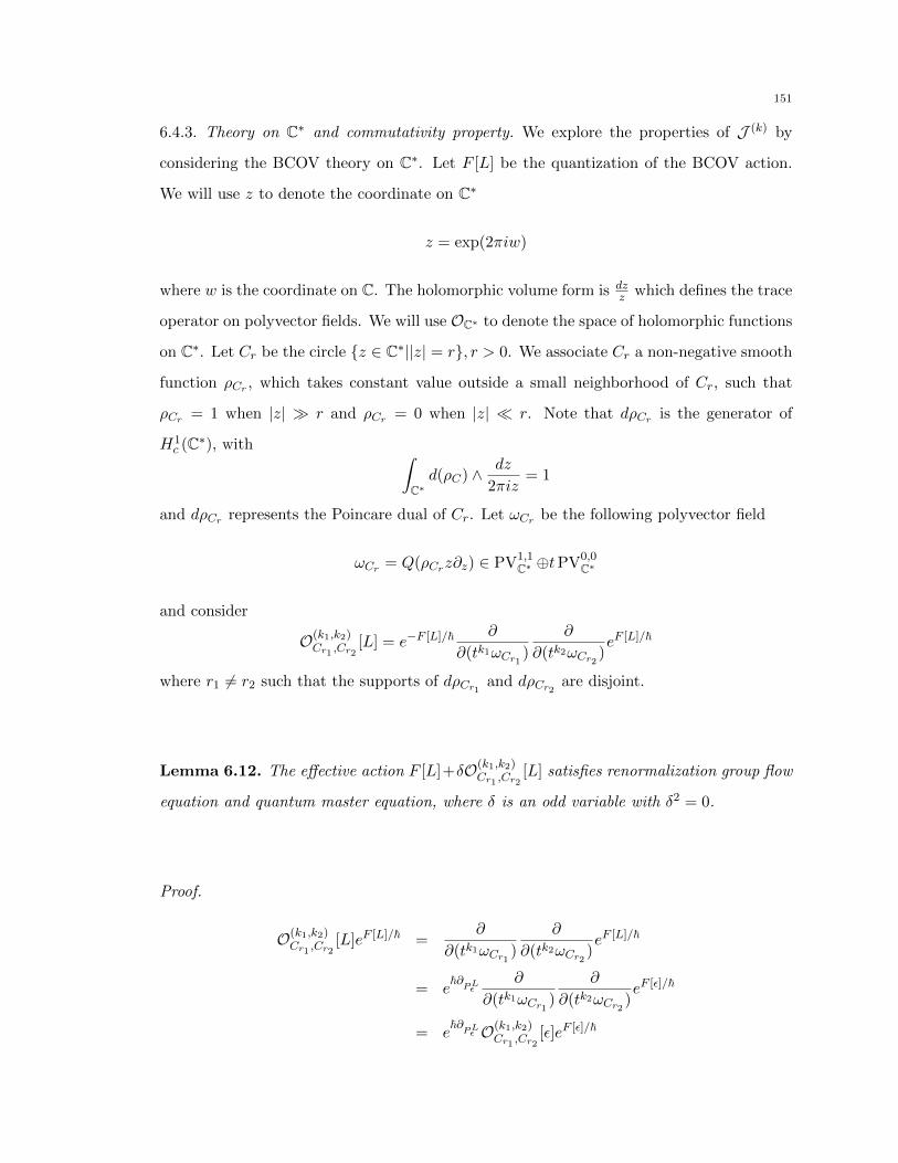
151

6.4.3. Theory on C∗ and commutativity property. We explore the properties of J (k) by

considering the BCOV theory on C∗. Let F [L] be the quantization of the BCOV action.

We will use z to denote the coordinate on C∗

z = exp(2πiw)

where w is the coordinate on C. The holomorphic volume form is dzz which defines the trace

operator on polyvector fields. We will use OC∗ to denote the space of holomorphic functions

on C∗. Let Cr be the circle z ∈ C∗||z| = r, r > 0. We associate Cr a non-negative smooth

function ρCr , which takes constant value outside a small neighborhood of Cr, such that

ρCr = 1 when |z| r and ρCr = 0 when |z| r. Note that dρCr is the generator of

H1c (C∗), with ∫

C∗d(ρC) ∧ dz

2πiz= 1

and dρCr represents the Poincare dual of Cr. Let ωCr be the following polyvector field

ωCr = Q(ρCrz∂z) ∈ PV1,1C∗ ⊕tPV0,0

C∗

and consider

O(k1,k2)Cr1 ,Cr2

[L] = e−F [L]/~ ∂

∂(tk1ωCr1 )

∂

∂(tk2ωCr2 )eF [L]/~

where r1 6= r2 such that the supports of dρCr1 and dρCr2 are disjoint.

Lemma 6.12. The effective action F [L]+δO(k1,k2)Cr1 ,Cr2

[L] satisfies renormalization group flow

equation and quantum master equation, where δ is an odd variable with δ2 = 0.

Proof.

O(k1,k2)Cr1 ,Cr2

[L]eF [L]/~ =∂

∂(tk1ωCr1 )

∂

∂(tk2ωCr2 )eF [L]/~

= e~∂PLε

∂

∂(tk1ωCr1 )

∂

∂(tk2ωCr2 )eF [ε]/~

= e~∂PLε O(k1,k2)

Cr1 ,Cr2[ε]eF [ε]/~

152

which proves the renormalization group flow equation. Since Q(tk1ωCr1 ) = Q(tk2ωCr2 ) = 0,

(Q+ ~∆L)O(k1,k2)Cr1 ,Cr2

[L]eF [L]/~ = (Q+ ~∆L)∂

∂(tk1ωCr1 )

∂

∂(tk2ωCr2 )eF [L]/~

=∂

∂(tk1ωCr1 )

∂

∂(tk2ωCr2 )(Q+ ~∆L) eF [L]/~

= 0

which proves the quantum master equation.

We will consider the restriction of O(k1,k2)Cr1 ,Cr2

[L] as a functional on OC∗ ⊂ PV0,0C∗ in the

following discussion, and we still denoted it by O(k1,k2)Cr1 ,Cr2

[L]. Since ωCr1 , ωCr2 have compact

support, we can take L → ∞ to obtain O(k1,k2)Cr1 ,Cr2

[∞] as a functional on OC∗ . Note that

elements in OC∗ lie in the kernel of Q = ∂ + t∂. Quantum master equation implies that

O(k1,k2)Cr1 ,Cr2

[∞] only depends on the homology class of Cr1 , Cr2 and the integers k1, k2 if we

restrict on OC∗ . Following the convention as in Eqn (6.58), we have the following

Lemma 6.13. Restricting on OC∗, then

O(k1,k2)Cr1 ,Cr2

[∞] = exp(~∂P∞0

)(∫C1

dz

2πizJ (k1)

∫C2

dz

2πizJ (k2)

)(6.60)

where PLε is the regularized BCOV propagator on C∗

PLε (z1, z2) = − 1

π

∫ L

ε

dt

4πt

∑n∈Z

(w1 − w2 + n

4t

)2

e−|w1−w2+n|2/4t

and

P∞0 (z1, z2) = limε→0L→∞

PLε (z1, z2) =1

(2πi)2

∑n∈Z

1

(w1 − w2 − n)2=

z1z2

(z1 − z2)2

here zk = exp(2πiwk), k = 1, 2.

Since O(k1,k2)Cr1 ,Cr2

[∞] only depends on the homology class of Cr1 , Cr2 , we have

exp(~∂P∞0

)(∫Cr1

dz1

2πiz1J (k1)

∫Cr2−Cr3

dz2

2πiz2J (k2)

)= 0

where 0 < r3 < r1 < r2. We call this the commutativity property.

153

Lemma 6.14. J (k)’s are uniquely determined (up to total derivative) by the initial condi-

tions J (k)(α) = 1(k+2)!α

k+2 +O(~), α ∈ OC∗ and the above commutativity property.

Proof. If the propagator connects one α(n) from J (k1)(α) and one α(m) from J (k2)(α), it

replaces the two terms by

~(√

~z1∂z1

)n (√~z2∂z2

)m z1z2

(z1 − z2)2= (−1)m+1

(√~z1∂z1

)n+m+1( √

~z2

z1 − z2

)

Using residue we see that

exp(~∂P∞0

)(∫C1

dz1

2πiz1J (k1)

∫C2−C′2

dz2

2πiz2J (k2)

)

gives rise to local functional∫C1

dz2πiz I where I(α) ∈ C[α, α(1), · · · ][

√~,√~−1

]. Let

u(n)(z1, z2) = −(√

~z1∂z1

)n( √~z2

z1 − z2

)

We claim that

u(n)u(m) =n!m!

(n+m+ 1)!u(n+m+1) +

√~f(u(k),

√~)

where f is a polynomial which is linear in u(k)’s. This can be proved by induction on n.

For n = 0,

u(0)u(m) =

√~z2

z1 − z2

(√~z1∂z1

)m( √~z2

z1 − z2

)We use power series to represent

u(m) =√~m+1

∞∑k=0

km(z1

z2

)kthen

u(0)u(m) =√~m+2

∞∑k=0

k∑j=0

jm(z1

z2

)k=√~m+2

∞∑k=0

P (k)

(z1

z2

)kwhere P (k) is a polynomial in k with the highest degree term given by 1

m+1km+1. This

proves the case for n = 0. The induction follows easily from the formula

u(n)u(m) =(√

~z1∂z1

)(u(n−1)u(m)

)− u(n−1)u(m+1)

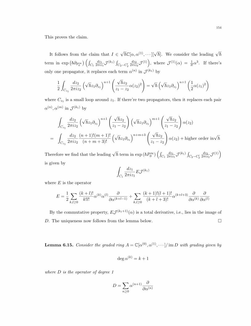
154

This proves the claim.

It follows from the claim that I ∈√~C[α, α(1), · · · ][

√~]. We consider the leading

√~

term in exp(~∂P∞0

) (∫C1

dz12πiz1J (k1)

∫C2−C′2

dz22πiz2J (1)

), where J (1)(α) = 1

3!α3. If there’s

only one propagator, it replaces each term α(n) in J (k1) by

1

2

∫Cz1

dz2

2πiz2

(√~z1∂z1

)n+1( √

~z2

z1 − z2α(z2)2

)=√~(√

~z1∂z1

)n+1(

1

2α(z1)2

)where Cz1 is a small loop around z1. If there’re two propagators, then it replaces each pair

α(n), α(m) in J (k1) by∫Cz1

dz2

2πiz2

(√~z1∂z1

)n+1( √

~z2

z1 − z2

)(√~z1∂z1

)m+1( √

~z2

z1 − z2

)α(z2)

=

∫Cz1

dz2

2πiz2

(n+ 1)!(m+ 1)!

(n+m+ 3)!

(√~z1∂z1

)n+m+3( √

~z2

z1 − z2

)α(z2) + higher order in

√~

Therefore we find that the leading√~ term in exp (~P∞0 )

(∫C1

dz12πiz1J (k1)

∫C2−C′2

dz22πiz2J (1)

)is given by ∫

C1

dz1

2πiz1EJ (k1)

where E is the operator

E =1

2

∑k,l≥0

(k + l)!

k!l!α(k)α(l) ∂

∂α(k+l−1)+∑k,l≥0

(k + 1)!(l + 1)!

(k + l + 3)!α(k+l+3) ∂

∂α(k)

∂

∂α(l)

By the commutative property, EJ (k1+1)(α) is a total derivative, i.e., lies in the image of

D. The uniqueness now follows from the lemma below.

Lemma 6.15. Consider the graded ring A = C[α(0), α(1), · · · ]/ imD with grading given by

degα(k) = k + 1

where D is the operator of degree 1

D =∑n≥0

α(n+1) ∂

∂α(n)

155

Let E be the operator of degree 2 acting on A

E =1

2

∑k,l≥0

(k + l)!

k!l!α(k)α(l) ∂

∂α(k+l−1)+∑k,l≥0

(k + 1)!(l + 1)!

(k + l + 3)!α(k+l+3) ∂

∂α(k)

∂

∂α(l)

There there exists unique J (k) ∈ A of degree k + 1 such that

EJ (k) = 0

Proof. Let E = E1 + E2 where

E1 =1

2

∑k,l≥0

(k + l)!

k!l!α(k)α(l) ∂

∂α(k+l−1),

E2 =∑k,l≥0

(k + 1)!(l + 1)!

(k + l + 3)!α(k+l+3) ∂

∂α(k)

∂

∂α(l)

It’s easy to check that

[D,E1] = [D,E2] = 0

We write E1 = E′1 +Dα(0), where

E′1 =1

2

∑k,l>0

(k + l)!

k!l!α(k)α(l) ∂

∂α(k+l−1)− α(1)

We can choose a basis of A = C[α(0), α(1), · · · ]/ imD as

α(i1)α(i2) · · · (α(ik))2, 0 ≤ i1 ≤ i2 ≤ · · · ≤ ik

then E′1 acts on the above basis in the obvious way, while for the action of E2, we need to

transform the result of the action to the above basis using the operator D.

Claim kerE′1 = Span(α(0)

)kk≥0.

To prove the claim, we consider the filtration by the numbers of α(1)

F pA =(α(1)

)pA,

156

then

E′1 ≡ α(1)

∑k≥2

(k + 1)α(k) ∂

∂α(k)+ α(1) ∂

∂α(1)− 1

: GrpF •A→ Grp+1F • A

where(∑

k≥2(k + 1)α(k) ∂∂α(k) + α(1) ∂

∂α(1) − 1)

is a rescaling operator on A, which is positive

on α(i1)α(i2) · · · (α(ik))2 if ik ≥ 1. For(α(0)

)k, we have

E′1

(α(0)

)k= −

(α(0)

)kα(1) = − 1

k + 1D(α(0)

)k+1

which is zero in A. This proves the claim.

Let A(k) be the degree k part of A which is finite dimensional. We consider the second

homogeneous grading on A(k) by giving all α(k) homogeneous degree 1. Then E′1 is homo-

geneous of degree 1 and E2 is homogeneous of degree −1. Let f ∈ A(k) such that Ef = 0.

We decompose

f =

k∑i=0

fi

where fk contains is homogeneous of degree i. Therefore we have

E1fk = 0, E1fk−1 = 0

E2fi = −E1fi−2 , 2 ≤ i ≤ k

It follows from the claim that fk is a multiple of(α(0)

)kand all the other fi’s are uniquely

determined. This proves the uniqueness.

To show the existence, we consider the lagrangian in Eqn (6.48)∫C

dz

2πiz

∑k≥−1

λk+1L(k)(α(z))

=

∫C

dz

2πizexp (S(λz∂z)(λα(z))) , S(t) =

sinh t/2

t/2

=

∫C

dz

2πizexp

((eλz∂z/2 − e−λz∂z/2

)φ(z))

), α(z) = z∂zφ(z)

=

∫C

dz

2πizexp

(φ(eλ/2z)− φ(e−λ/2z)

)=

∫C

dz

2πizexp

(φ(eλz)− φ(z)

)

157

=

∫C

dz

2πize−φ(z)eλz∂zeφ(z)

=

∫C

dz

2πiz

∑k≥0

λk

k!(z∂z + α)k · 1

where we use the convention that L(−1) = 1. Now we view α(z) as the bosonic field of the

free boson system described in section 6.2. Since the normal ordered operator

1

S(λ)

∫C

dz

2πiz: exp (S(λz∂z)(λα(z))) :B

is the bosonization of the fermionic operator∫C

dz

2πizb(eλ/2z)c(e−λ/2z)

which is already simultaneously diagonalized on the standard fermionic basis. It follows

that ∫C

dz

2πiz: L(k) :B

are commuting operators on the bosonic Fock space, where the normal ordering relation is

given by

α(z1)α(z2) =z1z2

(z1 − z2)2+ : α(z1)α(z2) :B if |z1| > |z2|

If we rescale λ→√~λ, then∫

C

dz

2πiz:

1

(k + 1)!(√~z∂z + α)k+11 :B

are commutating operators on bosonic Fock space if we impose the normal ordering relation

α(z1)α(z2) =~z1z2

(z1 − z2)2+ : α(z1)α(z2) :B if |z1| > |z2|

This is precisely the commutativity property, i.e., we can take

J (k) =1

(k + 1)!

(D + α(0)

)k+11 ∈ A

This proves the existence.

6.5. Proof of mirror symmetry. In this section, we prove Theorem 6.1.

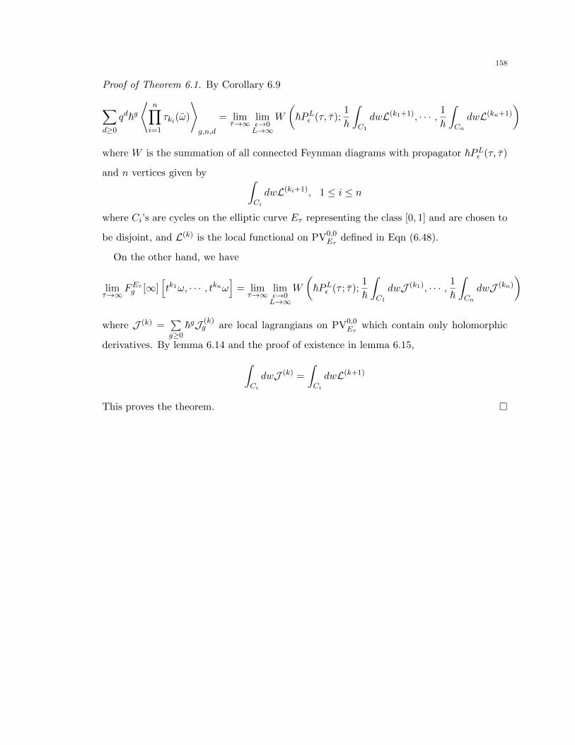
158

Proof of Theorem 6.1. By Corollary 6.9

∑d≥0

qd~g⟨

n∏i=1

τki(ω)

⟩g,n,d

= limτ→∞

limε→0L→∞

W

(~PLε (τ, τ);

1

~

∫C1

dwL(k1+1), · · · , 1

~

∫Cn

dwL(kn+1)

)

where W is the summation of all connected Feynman diagrams with propagator ~PLε (τ, τ)

and n vertices given by ∫Ci

dwL(ki+1), 1 ≤ i ≤ n

where Ci’s are cycles on the elliptic curve Eτ representing the class [0, 1] and are chosen to

be disjoint, and L(k) is the local functional on PV0,0Eτ

defined in Eqn (6.48).

On the other hand, we have

limτ→∞

FEτg [∞][tk1ω, · · · , tknω

]= lim

τ→∞limε→0L→∞

W

(~PLε (τ ; τ);

1

~

∫C1

dwJ (k1), · · · , 1

~

∫Cn

dwJ (kn)

)

where J (k) =∑g≥0

~gJ (k)g are local lagrangians on PV0,0

Eτwhich contain only holomorphic

derivatives. By lemma 6.14 and the proof of existence in lemma 6.15,∫Ci

dwJ (k) =

∫Ci

dwL(k+1)

This proves the theorem.

159

Appendix A. L∞ algebra

We will fix a ring R which contains Q. All algebras, modules and tensor products are

over R unless otherwise specified.

A.1. L∞ structure. Let g be a graded module

g =⊕n∈Z

gn

where gn has degree n. Consider the reduced graded symmetric product

S (g[1]) =⊕n≥1

Symn (g[1])(A.1)

where [1] is the shifting operator such that

g[1]n = gn+1

and Sym∗ is the graded symmetric product. S (g[1]) has a graded commutative co-algebra

structure. The co-product ∆ is given as follows: for any v1, · · · , vn ∈ g[1], v1v2 · · · vn gives

an element in Symn (g[1]), then

∆ : S (g[1]) → S (g[1])⊗R S (g[1])

v1v2 · · · vn → ∆ (v1v2 · · · vn) =∑

I⊂1,··· ,n

ε(I, Ic)vI ⊗ vIc(A.2)

here the summation is over all subset I of the indices 1, · · · , n, Ic is the complement

of I. For each I, we choose some order for elements in I, Ic. Then if I = i1, · · · , ik,

we write vI = vi1 · · · vik . ε(I, Ic) is the sign by permuting v1 · · · vn into the order vIvIc in

SymnR (g[1]). It’s easy to see that the formula doesn’t depend on the choice of the order in

I, Ic.

Definition A.1. A structure of L∞ algebra on g is given by a nilpotent coderivation of

degree one Q on S (g[1]) which satisfies

Q2 = 0, ∆Q = (Q⊗ 1 + 1⊗Q) ∆(A.3)

160

This is equivalent to saying that the triple(S (g[1]) ,∆, Q

)is a dg-coalgebra.

The L∞ structure Q is completely determined by

Qk : SymkR (g[1])

Q→ S (g[1])→ g[1](A.4)

where the last map is the projection to Sym1(g[1]) = g[1]. In fact, given v1, · · · , vn ∈ g[1],

we have

Q (v1 · · · vn) =∑

I⊂1,··· ,n

ε(I, Ic)Q|I| (vI) vIc(A.5)

where |I| is the size of I.

Definition A.2. A L∞ morphism between two L∞ algebras g, g′ is a degree zero homo-

morphism

F : S (g[1])→ S(g′[1]

)which is compatible with coproduct and coderivation, i.e.

(F ⊗ F ) ∆ = ∆′F, FQ = Q′F

where ∆,∆′ and Q,Q′ are the coproducts and coderivations on S (g[1]) and S (g′[1]) re-

spectively. In other words, F is a morphism of dg-coalgebras.

Similar to (A.4), F is determined by

Fk : Sk(g1[1])F→ S(g2[1])→ g2[1](A.6)

and for any v1, · · · , vn ∈ g1[1],

F (v1 · · · vn) =∑r

∑I1,··· ,Ir,

I1∪···∪Ir=1,··· ,n

ε(I1, · · · , Ir)r!

F|I1|(vI1) · · ·F|Ir|(vIr)(A.7)

Here the convention for ε(I1, · · · , Ir) is similar to (A.2).

Example A.3 (DGLA). A differential graded Lie algebra is a L∞ algebra g with Qk = 0

for k > 2. If x ∈ g, we will use deg(x) to denote the degree of x, and x[1] to denote the

161

corresponding element of g[1]. We define a differential on g by requiring

(dx) [1] = −Q1 (x[1])

and a bracket [, ] on g by requiring

([x, y]) [1] = (−1)deg(x)Q2 (x[1]y[1])

Now we explore the condition Q2 = 0. For any x ∈ g,

Q2 (x[1]) = Q21x[1] =

(d2x)

[1] = 0

which implies that

d2 = 0

For any x, y ∈ g,

Q (x[1]y[1]) = (−1)(deg(x)+1)(deg(y)+1)Q (y[1]x[1])

which implies that

[x, y] = −(−1)deg(x) deg(y)[y, x]

Q2 (x[1]y[1]) = Q1Q2 (x[1]y[1]) +Q2

((Q1x[1]) y[1] + (−1)deg(x)+1x[1] (Q1y[1])

)= −(−1)deg(x) (d[x, y]) [1]− (−1)deg(x)+1 ([dx, y]) [1] + ([x, dy]) [1]

= 0

which implies that

d[x, y] = [dx, y] + (−1)deg(x)[x, dy]

For any x, y, z ∈ g,

Q22 (x[1]y[1]z[1]) = Q2 ((Q2(x[1]y[1])) z[1]) + (−1)deg(x)+1Q2 (x[1] (Q2(y[1]z[1])))

+(−1)(deg(y)+1) deg(x)Q2 (y[1] (Q2(x[1]z[1])))

= (−1)deg(y)[[x, y], z][1] + (−1)deg(y)+1[x, [y, z]][1]

+(−1)deg(x) deg(y)+deg(y)[y, [x, z]][1]

162

= 0

which implies

[[x, y], z] = [x, [y, z]]− (−1)deg(x) deg(y)[y, [x, z]]

It’s easy to see that all the other relations in Q2 = 0 will follow from the above identities.

Therefore L∞ algebra structure with Qk = 0 for k > 2 is equivalent to the differential

graded Lie algebra structure.

Example A.4 (Differential forms on graded commutative algebra). Let A be a graded

commutative k-algebra, where k is the base field. The tangent space is defined to be the

space of graded k-derivation

TA = Derk(A)

Given D ∈ TA, we will use |D| to denote its degree as a map of graded vector spaces. Then

D(ab) = (Da)b+ (−1)|D||a|aDb ∀a, b ∈ A

TA has a natural structure of graded Lie algebra, with the Lie structure given by

[D1, D2] = D1D2 − (−1)|D1||D2|D2D1

and left A-module structure with

(aD)(b) = aD(b) ∀a, b ∈ A

The differential forms are defined by

Ω∗A = HomA (S (TA[1]) , A) =⊕n≥0

SymnA

(Ω1A

)where S (TA[1]) =

∏n≥0

SymnA (TA[1]) and Ω1

A = HomA(TA[1], A) is the space of Kahler

differentials.

Here we use the following convention for the shifting operator [1]: if M is a graded A-

module, M [1] is the degree one shifting of M , then the A-module structure on M [1] is given

by

a · (m[1]) = (−1)|a|(am)[1], ∀a ∈ A,m ∈M

163

Ω∗A can be viewed as the Chevalley-Eilenberg complex of the graded Lie algebra TA

valued in A, which is naturally a TA-module. It is endowed with the Chevalley-Eilenberg

differential d, which is also uniquely determined through the following

(1) If f ∈ Ω0A ≡ A, then df ∈ Ω1

A is determined by

df(X[1]) = (−1)|X|X(f)

for X ∈ TA. By our convention, df is obviously A-linear.

(2) d2 = 0

(3) d (αβ) = (dα)β + (−1)|α|αdβ, for any α, β ∈ Ω∗A.

A.2. Maurer-Cartan equation.

Definition A.5. Let g be a L∞ algebra, b ∈ g[1]0 = g1. The Maurer-Cantan equation for

b is defined to be

∑k≥1

1

k!Qk

(bk)

= 0(A.8)

We will use the notation

Q∗ =∑k≥1

Qk : S(g[1])→ g[1], eb =∑k

bk

k!

Then the Maurer-Cartan equation can be written as

e−bQ∗(eb) = 0(A.9)

Let F : (g, Q1)→ (g′, Q2) be a L∞ morphism of L∞ algebras. We will denote by

F∗ =∑k

Fk : S(g[1])→ g′[1]

then

F (eb) = F (∑k

bk

k!)

=∑k

∑r

1

r!

∑i1,··· ,ir,i1+···+ir=k

Fi1(bi1) · · ·Fir(bir)i1! · · · ir!

164

= eF∗(eb)

Therefore

Q′∗(eF∗(eb)) = Q′∗F (eb) = F∗Q(eb) = F∗(Q∗(e

b)eb)

hence the morphism

b→ F∗(eb)

preserves the solutions of Maurer-Cartan equation.

Definition A.6. The Maurer-Cartan functor of a L∞ algebra g is the functor

MCg : graded commutative Artin algebra → sets

A→MCg(A) =

b ∈ (g⊗mA) [1]0|

∑k≥1

1k!Qk

(bk)

= 0

from graded commutative Artin algebras to sets, which sends A to the space of solutions

of Maurer-Cartan equations of g⊗mA. Here mA is the nilpotent maximal ideal of A.

MCg is indeed a functor since we have seen that morphism of L∞ algebras preserves the

solutions of Maurer-Cartan equations.

MCg can also be understood from the viewpoints of functor of points. Let A a graded

commutative Artin R-algebra, with mA the maximal ideal. The dual m∨A has a natural co-

product structure which we denote by ∆m∨A, and we endow m∨A with the zero co-derivation.

Let b ∈ (g⊗mA) [1]0, which can be identified with the morphism of graded vector spaces

b : m∨V → g[1]

and it induces a morphism of graded co-algebras

∑k≥1

bk

k!∆k−1m∨A

: m∨V → S (g[1])

here ∆km∨A

is defined to be

∆km∨A

=(

∆m∨A⊗ 1⊗k−1

)(∆m∨A

⊗ 1⊗k−2)· · ·(

∆m∨A⊗ 1)

∆m∨A

165

and we have ∆km∨A

= 0 for k sufficiently large since mA is nilpotent. Then the condition for

b satisfying Maurer-Cartan equation says precisely that the map∑k≥1

bk

k! ∆k−1m∨A

is a morphism

of dg-coalgebras. Therefore

MCg(A) = HomDGC

(m∨A, S (g[1])

)where DGC refers to dg-coalgebra.

Example A.7. If g is a DGLA. Let x ∈ g1. The Maurer-Cartan equation is

Q1(x[1]) +1

2Q2 (x[1]x[1]) = 0

which is equivalent to

dx+1

2[x, x] = 0

This can be viewed as the deformation of the differential d to

d→ dx = d+ [x,−]

and Maurer-Cartan equation says that d2x = 0.

A.3. Homotopy. Let g be a L∞ R-algebra. We consider the graded vector spaces

g[t, dt]

Here t be a variable of degree 0, and dt is of degree 1. We have an induced dg-coalgebra

structure on

S (g[1][t, dt])

The co-derivation is given by

Q+ dt

where Q is the co-derivation induced from that on S (g[1]) and dt = dt ∧ ∂∂t . This gives a

L∞ structure on g[t, dt]. For t0 ∈ R, we have the evaluation map of L∞ algebras

Evalt=t0 : g[t, dt] → S (g)

P (t) +Q(t)dt → P (t0)

166

Definition A.8. Two L∞ homomorphisms F1, F2 : g → g′ are said to be homotopic to

each other, if there exists a L∞ morphism F : g→ g′[t, dt] such that F1 = Evalt=0 F and

F2 = Evalt=1 F . A L∞ homomorphism F : g→ g′ is said to be homotopy equivalence

if there exists a L∞ morphism G : g′ → g such that the compositions F G and G F are

homotopic to identities.

Proposition A.9. If F : g→ g′ is a L∞ homomorphism which induces a quasi-isomorphism

of complexes

F :(S (g[1]) , Q1

)→(S(g′[1]

), Q′1

)then F is a homotopy equivalence.

Proof. See for example [Kon03, Fuk].

A.4. Deformation functor.

Definition A.10. Let g be a L∞ algebra, and b1, b2 be two elements of g[1]0 which satisfy

the Maurer-Cartan equation. We say that b1 is gauge equivalent to b2 if there exists b ∈

(g[1][t, dt])0 such that b satisfies Maurer-Cartan equation and Evalt=0(b) = b1,Evalt=1(b) =

b2.

Example A.11. Let’s consider the case that g is a DGLA. Let x(t) + y(t)dt be an element

of g[t, dt] which solves the Maurer-Cartan equation. Then

(d+ dt) (x(t) + y(t)dt) +1

2[x(t) + y(t)dt, x(t) + y(t)dt] = 0

or equivalently

dx(t) + 12 [x(t), x(t)] = 0

∂∂tx(t) = dy(t) + [x(t), y(t)]

If we write dx(t) = d+ [x(t),−], then the above equations can be rewritten as

d2x(t) = 0,

∂

∂tdx(t) = [dx(t), [y(t),−]]

167

Given a L∞ algebra, we define its deformation functor by

Defg : graded commutative Artin R-algebra → sets

A→ Defg(A) =MCg(A)/ ∼

where the equivalence relation ∼ is the gauge equivalence.

In explicit deformation problems, the deformation functor is usually realized as a defor-

mation functor of certain L∞ algebra. The good thing about L∞ structure is that homotopy

equivalent L∞ algebras characterize essentially the same deformation space. More precisely

Proposition A.12. If g is homotopy equivalent to g′ as L∞ algebras, then the deformation

functor Defg is equivalent to the deformation functor Defg′.

Proof. See for example [Kon03, Fuk].

Appendix B. D-modules and Jets

Throughout this section, X will be a smooth oriented manifold of dimension n, and E

will be a graded vector bundle on X.

B.1. D-module. Let DX denote the sheaf of algebra of differential operators. If we choose

local coordinates x1, · · · , xn on X, then a local section of DX can be written as

∑I

fI(x)∂

∂xI

where I = i1, · · · , in is a multi-index, ∂∂xI

=(

∂∂x1

)i1· · ·(

∂∂xn

)in, and fI(x) is zero for all

but finitely many I’s.

Definition B.1. A DX-module is a sheaf of DX modules on X.

Example B.2. DX can be viewed as a free DX -module of rank 1, where the DX -module

structure is given by composition of differential operators.

Example B.3. The sheaf of smooth functions on X, which we denote by C∞(X), is

naturally a left DX -module.

168

Example B.4. If E is a vector bundle on X with a flat connection ∇, then E can be

viewed as a left DX -module. Locally, the DX -module structure is generated by

DX → End(E)

∂

∂xi→ ∇xi

Example B.5. Let X be an oriented smooth manifold, ωX be the sheaf of smooth top-

forms on X. Then ωX has the structure of right DX -modules. Given a section α of ωX , α

is uniquely determined by the map

α : C∞c (X) → C

f →∫Xαf

where C∞c (X) is the space of smooth functions with compact supports. Let P be a differ-

ential operator, then the right action of P on α is defined by requiring

α · P : C∞c (X) → C

f →∫XαP (f)

Example B.6 (Tensor product). Let M,N be two left DX -modules, we can define the

tensor product as a left DX -module by

M ⊗C∞(X) N

The DX -module structure is generated locally by

∂xi (m⊗ n) = (∂xim)⊗ n+m⊗ ∂xin

where m,n are sections of M,N respectively.

Definition B.7. Let M be a left DX -module. The de Rham complex of M is the defined

to be the complex

Ω∗X(M) ≡ Ω∗X ⊗C∞(X) M

169

where the differential is defined by

d (ω ⊗m) = (dω)⊗m+∑i

dxi ∧ ω ⊗ ∂xim(B.1)

Example B.8. There’s a natural complex of right DX -modules

0→ Ω0X ⊗C∞(X) DX → Ω1

X ⊗C∞(X) DX → · · · → ΩnX ⊗C∞(X) DX → ωX → 0

where the last morphism is determined via

α⊗ P : C∞c (X) → C

f →∫XαP (f)

which defines an element of ωX . It turns out that the above complex is exact, therefore we

have obtained the quasi-isomorphism of complexes of right DX -modules

ωX ' Ω∗X(DX)[n](B.2)

where n is the dimension of X.

B.2. Jet bundles. Let E be a vector bundle on X. We will not distinguish between E as

a vector bundle or E as a locally free sheaf. The sheaf of jets Jet(E) is locally given by

fαI eαI

where eα is a local basis of E, I = i1, · · · , inIi∈Z≥0 runs over the set of multi-indices,

and fαI is a local smooth function. There’s a natural map

Γ(E)→ Jet(E)

which in local coordinates x1, · · · , xn is

fαeα → ∂IfαeαI

here ∂If = ∂∂xI

f . There’s a natural DX -module structure on Jet(E) generated by

∂i∂IfαeαI = ∂ifαI eα − fαiIeαI

170

which gives the exact sequence of sheaves

0→ E → Jet(E)→ Ω1X(Jet(E))→ Ω2

X(Jet(E))→ · · ·

or equivalently we have the quasi-isomorphism of complex of C∞(X) sheaves

E ' Ω∗X(Jet(E))

There’s an intrinsic way to describe Jet(E) as follows. We consider the product X ×X

with two projections p1, p2

X ×Xp1

wwww

wwww

w p2

##GGGG

GGGG

G

X X

Let ∆ → X ×X be the diagonal, and I∆ be the ideal sheaf of ∆. Then

Jet(E) = lim←−k

p1∗

(C∞(X ×X)/Ik∆ ⊗ p∗2E

)and the DX -module structure comes from the natural action of differential operators on

the left copy X of X×X. If we choose local coordinates x1, · · · , xn on an open subset U of

X, a local basis eα of E, and let x′1, · · · , x′n be another copy of x1, · · · , xn, then xi, x′i

is a local coordinate system of U × U . Then

Jet(E)|U = C∞(U)[[δx1, · · · , δxn]]⊗ SpanC eα

where δxi = x′i − xi. An element of Jet(E)|U can be described by fαI eαI via

fαI (x)eαI →∑I

fI(x)δxI

I!eα

where δxI = δxi11 · · · δxinn , I! = i1! · · · in! if I = i1, · · · , in. The map E → Jet(E) is simply

given by the Taylor series

fα(x)eα → fα(x′)eα =∑I

fI(x)δxI

I!eα

171

We can also consider the projective dual

Jet(E)∨ = HomC∞(X)(Jet(E), C∞(X))

In local coordinates, if we represent an element of Jet(E) by

f =∑I

fαIδxI

I!eα ∈ C∞M (E)[[x1, · · · , xn]]

and represent an element of Jet(E)∨ by

g = gIα∂

∂xIeα

where eα is the dual basis of eα. Then we have the natural pairing

< g, f >=∑I,α

gIαfαI

Since both Jet(E) and C∞(X) have the structure of DX -modules, we have an induced

DX -module on Jet(E)∨. More precisely, in local coordinates, the action of ∂xi on Jet(E)∨

is given by requiring

∂xi < g, f >=< ∂xig, f > + < g, ∂xif >

from which we find

∂x

(gIα

∂

∂xIeα)

= ∂igIα

∂

∂xIeα + gIα

∂

∂xi∂

∂xIeα

This is exactly the natural DX -module structure that we would expect. In particular, it

shows that Jet(E)∨ is a locally free DX -module whose ranks equals the rank of the vector

bundle E.

We can also describe differential operators in terms of jet bundles. Let E,F be two

vector bundles on X, then the differential operators from E to F , denoted by Diff(E,F ),

is just a DX morphism from Jet(E) to Jet(F ) [Cos11]

Diff(E,F ) ∼= HomDX (Jet(E), Jet(F ))(B.3)

172

In fact, given ϕ ∈ HomDX (Jet(E), Jet(F )), it induces a differential operator Pϕ ∈ Diff(E,F ) ⊂

HomC (E,F ) from the following commutative diagram

0 // E //

Pϕ

Jet(E) //

ϕ

Ω1X(Jet(E)) //

1⊗ϕ

· · ·

0 // F // Jet(F ) // Ω1X(Jet(F )) // · · ·

B.3. Local functionals. Let

E = Γ(X,E)

be the space of smooth sections in E. Recall that a local functional on E of order k is given

by a map

S : Symk E → C

which takes the form

S[α1, · · · , αn] =

∫XD1(α1) · · ·Dk(αk)dVol

where αi ∈ E , Di : E → C∞(X) are some smooth differential operators, and dVol is a

volume form. It’s easy to see that such local functional can be described in terms of jet

bundle by

ωM ⊗DM SymkC∞(X)(Jet(E)∨)

where the tensor product over DM takes care of the fact that total derivatives are zero. It

follows that the space of local functionals can be described by

Oloc(E ) = ωX ⊗DX∏k≥1

SymkC∞(X)(Jet(E)∨)

where we have neglected the constant functional when k = 0. Since Jet(E)∨ is free DM -

module, the Koszul resolution (B.2) gives the quasi-isomorphism

Oloc(E ) ∼= Ω∗X

(Sym

∗≥1

C∞(X)(Jet(E)∨))

[n]

References

[ABK08] Mina Aganagic, Vincent Bouchard, and Albrecht Klemm, Topological strings and (almost)

modular forms, Comm. Math. Phys. 277 (2008), no. 3, 771–819.

[AS92] Scott Axelrod and I. M. Singer, Chern-Simons perturbation theory, Proceedings of the XXth

International Conference on Differential Geometric Methods in Theoretical Physics, Vol. 1, 2

(New York, 1991), World Sci. Publ., River Edge, NJ, 1992, pp. 3–45.

[AS94] , Chern-Simons perturbation theory. II, J. Differential Geom. 39 (1994), no. 1, 173–213.

[BCOV94] M. Bershadsky, S. Cecotti, H. Ooguri, and C. Vafa, Kodaira-Spencer theory of gravity and

exact results for quantum string amplitudes, Comm. Math. Phys. 165 (1994), no. 2, 311–427.

[BEK06] Spencer Bloch, Helene Esnault, and Dirk Kreimer, On motives associated to graph polynomials,

Comm. Math. Phys. 267 (2006), no. 1, 181–225.

[Ber87] Felix Alexandrovich Berezin, Introduction to superanalysis, Mathematical Physics and Applied

Mathematics, vol. 9, D. Reidel Publishing Co., Dordrecht, 1987.

[BF97] K. Behrend and B. Fantechi, The intrinsic normal cone, Invent. Math. 128 (1997), no. 1,

45–88.

[BK98] Sergey Barannikov and Maxim Kontsevich, Frobenius manifolds and formality of Lie algebras

of polyvector fields, Internat. Math. Res. Notices (1998), no. 4, 201–215.

[CdlOGP91] Philip Candelas, Xenia C. de la Ossa, Paul S. Green, and Linda Parkes, A pair of Calabi-Yau

manifolds as an exactly soluble superconformal theory, Nuclear Phys. B 359 (1991), no. 1,

21–74.

[CL] Kevin Costello and Si Li, Quantum BCOV theory on Calabi-Yau manifolds and the higher

genus B-model.

[Cos] Kevin Costello, A geometric construction of the witten genus, I, arXiv:math.QA/1006.5422.

[Cos09] , The partition function of a topological field theory, J. Topol. 2 (2009), no. 4, 779–822.

[Cos11] , Renormalization and effective field theory, Mathematical Surveys and Monographs,

vol. 170, American Mathematical Society, Providence, RI, 2011.

[CV91] Sergio Cecotti and Cumrun Vafa, Topological–anti-topological fusion, Nuclear Phys. B 367

(1991), no. 2, 359–461.

173

174

[Dij95] Robbert Dijkgraaf, Mirror symmetry and elliptic curves, The moduli space of curves (Texel

Island, 1994), Progr. Math., vol. 129, Birkhauser Boston, Boston, MA, 1995, pp. 149–163.

[EHX97] Tohru Eguchi, Kentaro Hori, and Chuan-Sheng Xiong, Quantum cohomology and Virasoro

algebra, Phys. Lett. B 402 (1997), no. 1-2, 71–80.

[Fuk] Kenji Fukaya, Deformation theory, homological algebra and mirror symmetry, Geometry and

physics of branes (Como, 2001), Ser. High Energy Phys. Cosmol. Gravit., pp. 121–209.

[Giv98] Alexander Givental, A mirror theorem for toric complete intersections, Topological field theory,

primitive forms and related topics (Kyoto, 1996), Progr. Math., vol. 160, Birkhauser Boston,

Boston, MA, 1998, pp. 141–175.

[Kac98] Victor Kac, Vertex algebras for beginners, second ed., University Lecture Series, vol. 10, Amer-

ican Mathematical Society, Providence, RI, 1998.

[Kon94] Maxim Kontsevich, Feynman diagrams and low-dimensional topology, First European Congress

of Mathematics, Vol. II (Paris, 1992), Progr. Math., vol. 120, Birkhauser, Basel, 1994, pp. 97–

121.

[Kon95a] , Enumeration of rational curves via torus actions, The moduli space of curves (Texel

Island, 1994), Progr. Math., vol. 129, Birkhauser Boston, Boston, MA, 1995, pp. 335–368.

[Kon95b] , Homological algebra of mirror symmetry, Proceedings of the International Congress

of Mathematicians, Vol. 1, 2 (Zurich, 1994) (Basel), Birkhauser, 1995, pp. 120–139.

[Kon03] , Deformation quantization of Poisson manifolds, Lett. Math. Phys. 66 (2003), no. 3,

157–216.

[KZ95] Masanobu Kaneko and Don Zagier, A generalized Jacobi theta function and quasimodular

forms, The moduli space of curves (Texel Island, 1994), Progr. Math., vol. 129, Birkhauser

Boston, Boston, MA, 1995, pp. 165–172.

[Li] Si Li, BCOV theory on elliptic curves and higher genus mirror symmetry.

[LLY97] Bong H. Lian, Kefeng Liu, and Shing-Tung Yau, Mirror principle. I, Asian J. Math. 1 (1997),

no. 4, 729–763.

[LT98] Jun Li and Gang Tian, Virtual moduli cycles and Gromov-Witten invariants of algebraic va-

rieties, J. Amer. Math. Soc. 11 (1998), no. 1, 119–174.

175

[MJD00] T. Miwa, M. Jimbo, and E. Date, Solitons, Cambridge Tracts in Mathematics, vol. 135, Cam-

bridge University Press, Cambridge, 2000, Differential equations, symmetries and infinite-

dimensional algebras, Translated from the 1993 Japanese original by Miles Reid.

[OP06a] A. Okounkov and R. Pandharipande, Gromov-Witten theory, Hurwitz theory, and completed

cycles, Ann. of Math. (2) 163 (2006), no. 2, 517–560.

[OP06b] , Virasoro constraints for target curves, Invent. Math. 163 (2006), no. 1, 47–108.

[RT94] Yongbin Ruan and Gang Tian, A mathematical theory of quantum cohomology, Math. Res.

Lett. 1 (1994), no. 2, 269–278.

[Sch93] Albert Schwarz, Geometry of Batalin-Vilkovisky quantization, Comm. Math. Phys. 155 (1993),

no. 2, 249–260.

[Tod89] Andrey N. Todorov, The Weil-Petersson geometry of the moduli space of SU(n ≥ 3) (Calabi-

Yau) manifolds. I, Comm. Math. Phys. 126 (1989), no. 2, 325–346.

[Wit88] Edward Witten, Topological sigma models, Comm. Math. Phys. 118 (1988), no. 3, 411–449.

[Wit92] , Mirror manifolds and topological field theory, Essays on mirror manifolds, Int. Press,

Hong Kong, 1992, pp. 120–158.

[Zin93] Aleksey Zinger, The reduced genus-one gromov-witten invariants of calabi-yau hypersurfaces,

arXiv:math.AG/0705.2397.