Caixia Cai, Nikhil Somani, Alois Knoll · Orthogonal Image Features for Visual Servoing of a 6 DOF...
9
1 Orthogonal Image Features for Visual Servoing of a 6 DOF Manipulator with Uncalibrated Stereo Cameras Caixia Cai, Nikhil Somani, Alois Knoll Abstract—We present an approach to control a 6 DOF manipulator using an uncalibrated visual servoing (VS) approach that addresses the challenges of choosing proper image features for target objects and designing a VS controller to enhance the tracking performance. The main contribution of this article is the definition of a new virtual visual space (image space). A novel stereo camera model employing virtual orthogonal cameras is used to map 6D poses from Cartesian space to this virtual visual space. Each component of the 6D pose vector defined in this virtual visual space is linearly independent, leading to a full-rank 6 × 6 image Jacobian matrix which allows avoiding classical problems, such as, image space singularities and local minima. Furthermore, the control for rotational and translational motion of robot are decoupled due to the diagonal image Jacobian. Finally, simulation results with an eye-to-hand robotic system confirm the improvement in controller stability and motion performance with respect to conventional VS approaches. Experimental results on a 6 DOF industrial robot are provided to illustrate the effectiveness of the proposed method and the feasibility of using this method in practical scenarios. Index Terms—Orthogonal Image Features, Visual Servoing. I. I NTRODUCTION Visual Servoing (VS) has been used in a wide spectrum of applications, from fruit picking to robotized surgery, and especially in industrial fields for tasks such as assembling, packaging, drilling and painting [1], [2]. According to the features used as feedback in minimizing the positioning error, visual servoing is classified into three categories [1]: Position- Based Visual Servoing (PBVS), Image-Based Visual Servoing (IBVS) and Hybrid Visual Servoing (HYVS). In general, a PBVS system has a good 3D trajectory but is sensitive to calibration errors. Compared to PBVS, IBVS is known to be robust to camera model errors [3] and the image feature point trajectories are controlled to move approximately along straight lines[4]. However, one of the main drawbacks of IBVS is that there may exist image singularities and image local minima leading to IBVS failure. The selection of visual features is a key point to solve the problem of image singularities. A great deal of effort has been dedicated to determine decoupling visual features that deliver a triangular or diagonal Jacobian matrix [5], [6]. In IBVS, geometric features in the image such as points, segments or straight lines [1] are usually chosen as image features and used as the inputs of controllers. Several novel features such as laser points [7], the polar signatures of an object contour [8], and image moments [6], [9], [10] have been developed to track objects which do not have enough detectable geometric features and to enhance the robustness of visual servoing systems. The image interaction matrix (image Authors Affiliation: Robotics and Embedded Systems Group, Technische Universit¨ at M¨ unchen, Germany. Email: {caica,somani,knoll}@in.tum.de Jacobian), can be computed using direct depth information [11], [12], by approximation via on-line estimation of depth of the features[13], [14], [15], [16], or using depth-independent image Jacobian matrix [17], [18]. Additionally, many papers directly estimate on-line the complete image Jacobian in dif- ferent ways [19], [20], [21], [22]. However, all these methods generally use redundant image point coordinates to define a non-square image Jacobian leading to well-known problems such as image singularities. It is also possible to combine the advantages of 2D and 3D visual servoing while avoiding their respective drawbacks. This approach is called 2-1/2D visual servoing because the used input is expressed partly in the 3D Cartesian space and partly in the 2D image space [23]. Contrary to PBVS, the 2- 1/2D approach does not need any geometric 3D model of the object. In comparison to IBVS, the 2-1/2D approach ensures the convergence of the control law in the whole task space. In this paper, we propose a new 2-1/2D visual servoing (coined 6DVS) which extracts new orthogonal image features and decouples the translational and the rotational control of a robot under visual feedback from fixed stereo cameras. More precisely, instead of using the classical visual features, we define a new virtual visual space (image space), where a 3D position vector is extracted as a feature. Each principal component of the position vector is linearly independent and orthogonal. We compute the orientation through a rotation matrix with Euler angles representation. We thus obtain a diagonal interaction matrix with very satisfactory decoupling properties. It is interesting to note that this Jacobian matrix has no singularity in the whole task space and the controls for the position and orientation are independent. Simulations and experimental results confirm that this new formulation (6DVS) is more efficient than existing classic VS approaches and the errors in both the virtual visual space and Cartesian space converge without local minima 1 . Moreover, it is less sensitive to image noise than classical 2-1/2D visual servoing. In Section II we formulate the classical 2-1/2D VS ap- proach, highlight its shortcomings and state the core issues. In Section III we introduce a new camera model to construct a virtual visual space and define a visual pose vector whose elements are chosen as image features. Using this 6D visual pose, a square full-rank image Jacobian is obtained, which is used in Section IV to simulate an adaptive 6D visual servoing controller and evaluate its properties. Section V presents two real-world experiments (Fig. 1) and shows the results obtained in a dynamic environment. Finally, Section VI presents the 1 Parts of this work have already been presented at IROS’14 [24]. In this paper, quantitative validations of the approach and comparisons to classical methods in terms of steady state errors, transient systems performance and robustness to uncertainties have been added.
Transcript of Caixia Cai, Nikhil Somani, Alois Knoll · Orthogonal Image Features for Visual Servoing of a 6 DOF...
1
Orthogonal Image Features for Visual Servoing of a 6 DOFManipulator with Uncalibrated Stereo Cameras
Caixia Cai, Nikhil Somani, Alois Knoll
Abstract—We present an approach to control a 6 DOFmanipulator using an uncalibrated visual servoing (VS) approachthat addresses the challenges of choosing proper image featuresfor target objects and designing a VS controller to enhance thetracking performance. The main contribution of this article isthe definition of a new virtual visual space (image space). Anovel stereo camera model employing virtual orthogonal camerasis used to map 6D poses from Cartesian space to this virtualvisual space. Each component of the 6D pose vector definedin this virtual visual space is linearly independent, leading toa full-rank 6× 6 image Jacobian matrix which allows avoidingclassical problems, such as, image space singularities and localminima. Furthermore, the control for rotational and translationalmotion of robot are decoupled due to the diagonal imageJacobian. Finally, simulation results with an eye-to-hand roboticsystem confirm the improvement in controller stability andmotion performance with respect to conventional VS approaches.Experimental results on a 6 DOF industrial robot are providedto illustrate the effectiveness of the proposed method and thefeasibility of using this method in practical scenarios.
Index Terms—Orthogonal Image Features, Visual Servoing.
I. INTRODUCTION
Visual Servoing (VS) has been used in a wide spectrumof applications, from fruit picking to robotized surgery, andespecially in industrial fields for tasks such as assembling,packaging, drilling and painting [1], [2]. According to thefeatures used as feedback in minimizing the positioning error,visual servoing is classified into three categories [1]: Position-Based Visual Servoing (PBVS), Image-Based Visual Servoing(IBVS) and Hybrid Visual Servoing (HYVS).
In general, a PBVS system has a good 3D trajectory but issensitive to calibration errors. Compared to PBVS, IBVS isknown to be robust to camera model errors [3] and the imagefeature point trajectories are controlled to move approximatelyalong straight lines[4]. However, one of the main drawbacksof IBVS is that there may exist image singularities andimage local minima leading to IBVS failure. The selectionof visual features is a key point to solve the problem of imagesingularities. A great deal of effort has been dedicated todetermine decoupling visual features that deliver a triangularor diagonal Jacobian matrix [5], [6].
In IBVS, geometric features in the image such as points,segments or straight lines [1] are usually chosen as imagefeatures and used as the inputs of controllers. Several novelfeatures such as laser points [7], the polar signatures of anobject contour [8], and image moments [6], [9], [10] havebeen developed to track objects which do not have enoughdetectable geometric features and to enhance the robustness ofvisual servoing systems. The image interaction matrix (image
Authors Affiliation: Robotics and Embedded Systems Group, TechnischeUniversitat Munchen, Germany. Email: {caica,somani,knoll}@in.tum.de
Jacobian), can be computed using direct depth information[11], [12], by approximation via on-line estimation of depthof the features[13], [14], [15], [16], or using depth-independentimage Jacobian matrix [17], [18]. Additionally, many papersdirectly estimate on-line the complete image Jacobian in dif-ferent ways [19], [20], [21], [22]. However, all these methodsgenerally use redundant image point coordinates to define anon-square image Jacobian leading to well-known problemssuch as image singularities.
It is also possible to combine the advantages of 2D and3D visual servoing while avoiding their respective drawbacks.This approach is called 2-1/2D visual servoing because theused input is expressed partly in the 3D Cartesian space andpartly in the 2D image space [23]. Contrary to PBVS, the 2-1/2D approach does not need any geometric 3D model of theobject. In comparison to IBVS, the 2-1/2D approach ensuresthe convergence of the control law in the whole task space.
In this paper, we propose a new 2-1/2D visual servoing(coined 6DVS) which extracts new orthogonal image featuresand decouples the translational and the rotational control of arobot under visual feedback from fixed stereo cameras. Moreprecisely, instead of using the classical visual features, wedefine a new virtual visual space (image space), where a3D position vector is extracted as a feature. Each principalcomponent of the position vector is linearly independent andorthogonal. We compute the orientation through a rotationmatrix with Euler angles representation. We thus obtain adiagonal interaction matrix with very satisfactory decouplingproperties. It is interesting to note that this Jacobian matrixhas no singularity in the whole task space and the controls forthe position and orientation are independent. Simulations andexperimental results confirm that this new formulation (6DVS)is more efficient than existing classic VS approaches and theerrors in both the virtual visual space and Cartesian spaceconverge without local minima 1. Moreover, it is less sensitiveto image noise than classical 2-1/2D visual servoing.
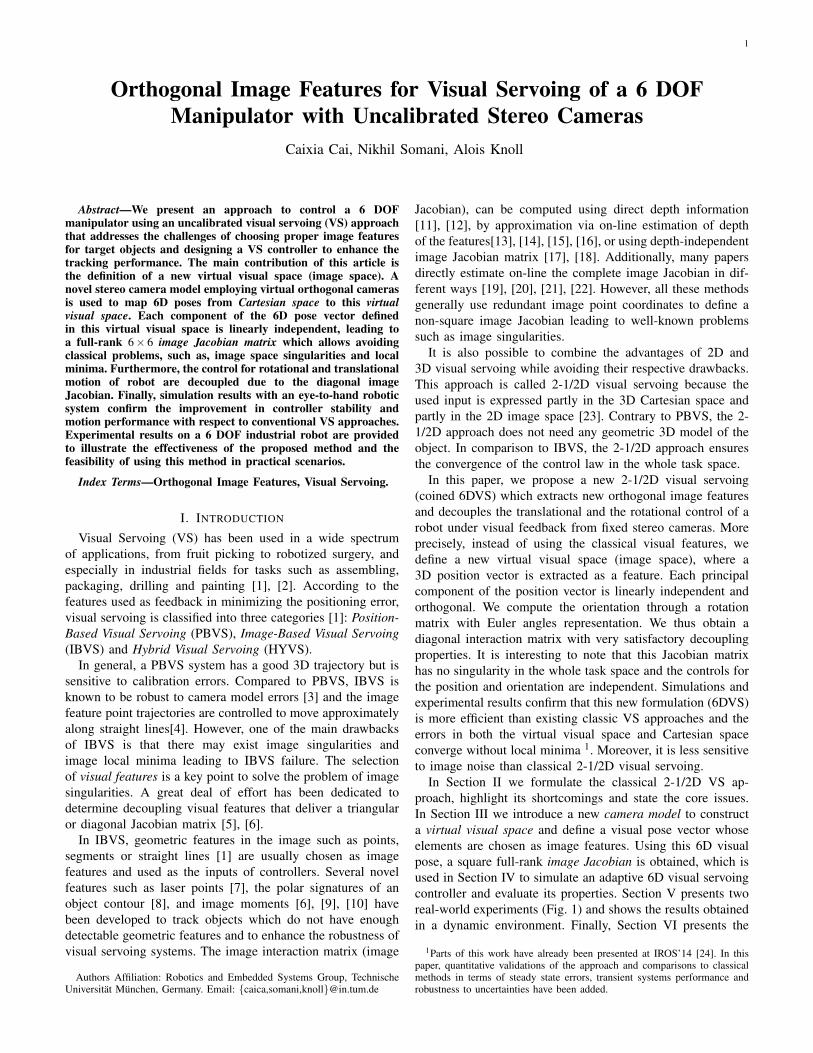
In Section II we formulate the classical 2-1/2D VS ap-proach, highlight its shortcomings and state the core issues.In Section III we introduce a new camera model to constructa virtual visual space and define a visual pose vector whoseelements are chosen as image features. Using this 6D visualpose, a square full-rank image Jacobian is obtained, which isused in Section IV to simulate an adaptive 6D visual servoingcontroller and evaluate its properties. Section V presents tworeal-world experiments (Fig. 1) and shows the results obtainedin a dynamic environment. Finally, Section VI presents the
1Parts of this work have already been presented at IROS’14 [24]. In thispaper, quantitative validations of the approach and comparisons to classicalmethods in terms of steady state errors, transient systems performance androbustness to uncertainties have been added.
2
DistributedSystem
VisualStereoTracker
RobotLow Level
Control
3DVisualization
System
2 cameras [Uncalibrated Stereo System] {30ms}
Virtual
Camera 1Virtual
Camera 2
t or qd
Voltage
q,qq,q
b) Top Viewa) General View VirtualObstacle
RobotEF
Target
Stereo System
Virtual
Camera 1Virtual
Camera 2Virtual
Obstacle
TCP/IP
{4 ms}
Fig. 1. Description of robotic experimental setup with fixed stereo cameras.
conclusions of our work and directions for future work.
II. PROBLEM FORMULATION
A. The Problem of Classical Methods
Suppose that the robot end-effector is moving with an-gular velocity ω = [ωx,ωy,ωz]
T and translational velocityv = [vx,vy,vz]
T both w.r.t. the camera frame in a fixed camerasystem (eye-to-hand configuration, see Fig. 1). Let Pc be apoint rigidly attached to the end-effector with X = [x,y,z]T .
In classical 2-1/2-D visual servoing, as described by Malis etal.[23], the selected feature vector is h= [XT
h ,θUT ]T , where Xhis the position vector, θ and U are the rotation angle and axisof the rotation matrix R. The corresponding image Jacobian isan upper block triangular matrix given by
J =
[ 1z Jv Jvω
03 Jω
]h = J
[vω
](1)
The position vector Xh = [u,v, ln(z)]T is defined in extendedimage coordinates, where u,v are the image features, 2Ddata (pixel) and z is the depth of the considered point, 3Ddata (meter). Moreover, according to image Jacobian (1),the translational velocity of the point Pc is affected by bothposition and orientation errors.
u and v are two orthogonal principal axes in image coor-dinates. If we can find a third, normalized zs component forimage coordinates which is orthogonal to u,v and measuredin pixels, then all the points in the image coordinates can bedecomposed into 3 principal components in such a way thatall the elements of the position vector can be controlled in alinearly independent way.
B. Design of proposed VS Features
Motivated by the desire to find a zs component of theposition vector which is also in the image plane (pixel) anddecouples the control of the translational and the rotationalmotion, we define a new virtual visual space (image space),where a 3D pixel position Xs is extracted as a feature. Allelements of this 3D position vector are linearly independentand orthogonal to each other. We solve the orientation using arotation matrix with ZY X Euler angles representation, denotedby θ . Thus, the new feature vector is Ws = [xs,ys,zs,α,β ,γ]T
and the new mapping is given by
Ws =
[Xsθ
]=
Jimg︷ ︸︸ ︷[Jv 0303 Jω
][vω
](2)
where the new image Jacobian (Jimg ∈ R6×6) is a decouplingdiagonal matrix that decouples the translational and rotationalcontrol.
III. 6D ADAPTIVE VISUAL SERVOING
Consider the motion of a plane π attached to the end effectorof a robot that rotates and translates through space in order toobtain a desired position and orientation of the end-effector.We define four target points on π denoted by Pi, ∀i = 1,2,3,4.In this work, we investigate the translational and rotationalmotion of the end-effector of a robot under visual feedbackfrom a fixed stereo camera system. By assuming knowledge ofthe camera intrinsic parameters, we obtain the pixel translationmotion using triangulation on the center of the four pointswhile utilizing the rotational information of the end-effectorthrough the motion of four tracked points.
The image Jacobian Jimg has a decoupled structure, whichis divided into position image Jacobian (Jv ∈ R3×3) andorientation image Jacobian (Jω ∈ R3×3).
A. Image Jacobian for 3D Position Jv
Since Xs ∈R3×1 represents the position in the image featurespace, the maximum number of independent elements forposition is 3. Hence, in this work we construct a virtual visualspace using the information generated from the stereo visionsystem where 3 linearly independent elements can be extractedto get a full-rank image Jacobian (Jv).
Jv ∈ R3×3 describes the relationship between the velocitiesof 3D Cartesian position Xb (meters) and 3D visual positionXs (pixels). The key idea of this model is to combine thestereo camera model with a virtual composite camera modelto get a full-rank image Jacobian, see Fig. 2.
This new 3D visual model can be computed in two steps:• The standard stereo vision model [25] is used to analyt-
ically recover the 3D relative position (XCl ) of an objectwith respect to the reference frame of the stereo systemOCl .
• The Cartesian position XCl is projected into two virtualcameras Ov1 and Ov2 .
1) Stereo Vision Model: Defining the observed imagepoints in each camera as pl = [ul ,vl ]
T , pr = [ur,vr]T , we
can use triangulation [25] to compute the relative positionXCl = [xc,yc,zc]
T with respect to the left camera OCl . Then theposition XCl can be mapped to the world frame Xb through
XCl = RbCl
Xb + tbCl
(3)
where T bc = [Rb
Cl, tb
Cl] is the transformation matrix between
coordinate frame OCl and Ob.Before integrating the stereo cameras model with the virtual
composite model, a re-orientation of the coordinate frame OClto a new coordinate frame OV with the same origin is required.The projection position XV = [xV ,yV ,zV ]
T with (3) is (Fig. 2)
XV = RClV XCl = RCl
V (RbCl
Xb + tbCl) (4)
where RClV is the orientation of the reference frame2 OV with
respect to OCl .
2This reference frame is fixed to the left camera coordinate frame and isdefined by the user, therefore RCl
V is assumed to be known.
3
Ov2
Ov1
Ocl
Ocr
pl
pr
pV2
pV1
Ob
X [m]b
Object
OV X ( )Cl XV
VirtualCameras
StereoSystem
RCl
V
X =R XV ClCl
V
RbCl
Ov is located at the same position as Ocl
vz
v
21 22
Xs=(u1, u2, v2)
o o
11 12o o
v1
v 1
v1v1
Xv=(xv, yv, zv) meterpixel
(u1,v1)
(u2,v2)
yv
(a) Composite Camera Model(b)
xv
x
yz
v
x
zy
v
v
v2
2
2
2
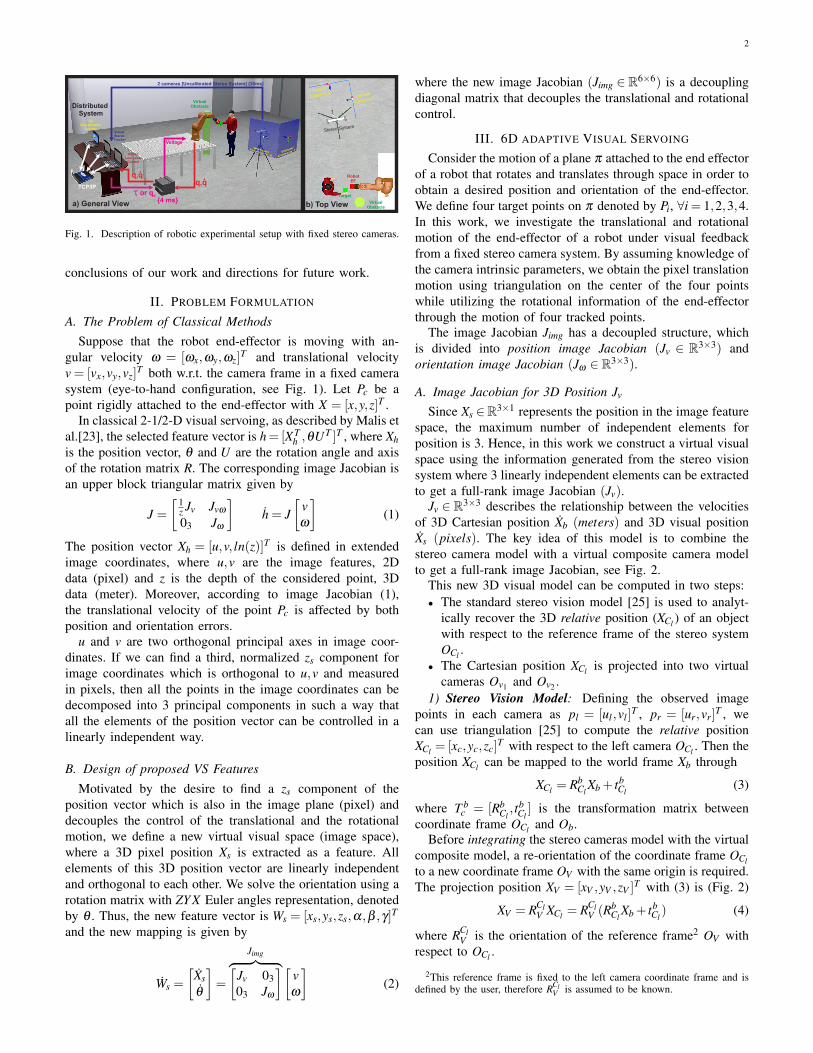
Fig. 2. Image projections: (a) The figure depicts the different coordinate frames used to obtain a general 3D virtual visual space. Xb ∈ R3×1 is the positionin meters [m] of an Object with respect to the world coordinate frame (wcf) denoted by Ob. Moreover, OCl and OCr are the coordinate frames for the leftand right cameras, respectively. Rb
Cl∈ SO(3) represents the orientation of wcf with respect to the left camera. OV is a reference coordinate frame for the
virtual orthogonal cameras Ov1,2 where RClV ∈ SO(3) is its orientation with respect to OCl . λ is the distance from Ovi to OV along each optical axis i. The
vectors pl , pr ∈R2×1 are the projections of the point Xb in the left and right cameras. Finally, pvi ∈R2×1 represents the projection of the Object in the virtualcameras Ovi . (b) Placement of the composite camera model with respect to left camera.
2) Virtual Composite Camera Model: In order to computethe 3D virtual visual space, we define two virtual camerasattached to the stereo camera system using the coordinateframe OV (Fig. 2 (b)). We use the pinhole camera model [25]to project the relative position XV to each of the virtual camerasOv1 and Ov2 .
The model for the virtual camera 1 is given by
pv1 =
[uv1
vv1
]=
1−yV +λ
αR(φ)
[xV −o11zV −o12
]+
[cxcy
]. (5)
where φ is the rotation angle of the virtual camera along itsoptical axis, O1 = [o11,o12]
T is the projected position of theoptical center with respect to the coordinate frame OV , C1 =[cx,cy]
T is the position of the principal point in image plane, λ
is the distance from the virtual camera coordinate frame Ov1to the reference frame OV along its optical axis. α and therotation matrix R(φ) are defined as:
α =
[f β 00 f β
]R(φ) =
[cosφ −sinφ
sinφ cosφ
]. (6)
where f is the focal length of the lens used and β is themagnification factor of the camera.
Since this model represents a user-defined virtual camera,all its parameters 3 are known in the defined configuration ofthe virtual cameras φ = 04 (Fig. 2 (b)).
Similarly, the model for virtual camera 2 is defined as:
pv2 =
[uv2vv2
]=
1xV +λ
αR(φ)
[yV −o21zV −o22
]+
[cxcy
]. (7)
In order to construct the 3D virtual visual space Xs ∈R3×1,we combine both virtual camera models.
3Since the virtual cameras are user-defined, we can set the same intrinsicparameters and λ values for both cameras.
4The reason to introduce the auxiliary coordinate frame OV is to simplifythe composite camera model by rotating the coordinate frame OCl in a specificorientation such as φ = 0.
Using properties of the rotation matrix R(φ) and the factthat α is a diagonal matrix, from (5), uv1 can be written in theform
uv1 = γ1xV −o11
−yV +λ− γ2vv1 + γ3 (8)
where the constant parameters γ1, γ2, γ3 ∈ R are explicitlydefined as
γ1 =f β
cosφ, γ2 = tan(φ), and γ3 = cx + cyγ2. (9)
Based on (7) and (8), we define a visual camera model (Os)representation Xs = [xs,ys,zs]
T using the orthogonal elements[uv1 ,uv2 ,vv2 ]
T as
Xs =
uv1uv2vv2
=
Rα︷ ︸︸ ︷[γ1 01×2
02×1 αR(φ)
]xV−o11−yV+λyV−o21xV+λ
zV−o22xV+λ
+ρ (10)
where ρ = [γ3− γ2vv1 ,cx,cy]T . The pixel position Xs constructs
the 3D virtual visual space.Given that φ = 0, then γ1 = f β , γ2 = 0, γ3 = cx, implies
that ρ = [cx,cx,cy]T and Rα = diag( f β ) ∈ R3×3. Therefore,
the mapping in (10) can be simplified as
Xs = diag( f β )
xV−o11−yV+λyV−o21xV+λ
zV−o22xV+λ
+ cx
cxcy
. (11)
The velocity mapping can be obtained with the time derivativeof (11) as follows:
Xs = Rα JoXV = Jα XV (12)
where the Jacobian matrix Jo ∈ R3×3 is defined as
Jo =
1
−yV+λ
xV−o11(−yV+λ )2 0
− yV−o21(xV+λ )2
1xV+λ
0− zV−o22
(xV+λ )2 0 1xV+λ
. (13)
4
Taking the time derivative of (4), (12) can be rewritten as
Xs = Jα(RClV Rb
Cl)Xb = JvXb (14)
where we define Jv ∈ R3×3 as the position image Jacobian.Remark 1: Virtual Cameras. The two virtual cameras are
selected in such a way that their optical axes intersect at 90degrees. Since the cameras are virtual they have infinite field ofview and pixel positions Xs can be either negative or positive.
B. Image Jacobian for 3D Orientation Jω
Let θ = [α,β ,γ]T be a vector of ZY X Euler angles, whichdenotes a minimal representation for the orientation of theend-effector frame relative to the robot base frame. Then, thedefinition of the angular velocity ω is given by [26]
ω = T (θ)θ . (15)
If the rotation matrix Re f = Rz,γ Ry,β Rx,α is the Euler angletransformation, then
T (θ) =
cos(γ)cos(β ) −sin(γ) 0sin(γ)cos(β ) cos(γ) 0−sin(β ) 0 1
(16)
Singularities of the matrix T (θ) are called representationalsingularities. It can easily be shown that T (θ) is invertibleprovided cos(β ) 6= 0.
Therefore,θ = T−1(θ)ω = Jω ·ω. (17)
where Jω ∈R3×3 is defined as the orientation image Jacobian.Combining (14) and (17) we have the full expression
Ws =
[Xsθ
]=
[Jv 00 Jω
][vω
](18)
= Jimg ·V (19)
where the matrix Jimg ∈ R6×6 is defined as the new imageJacobian, which is a block diagonal Jacobian matrix.
C. Control Scheme
Substituting the robot differential kinematics V = J(q)q,equation (19) can be rewritten in the form
Ws = JimgJ(q) · q = Js · q (20)
where J(q) ∈ R6×6 is the Jacobian matrix of the robotmanipulator and the matrix Js ∈R6×6 is defined as the visualJacobian.
According to (20) the corresponding control law is
qr = Js−1Wsr (21)
where qr is the joint velocity nominal reference and is usedin an adaptive second order sliding mode controller, which isdescribed in detail in the paper [27].
Remark 2: Singularity-free Jimg.From (18), we can see that det(Jimg) = det(Jv)det(Jω). Hence,the set of singular configurations of Jimg is the union of theset of position configurations satisfying det(Jv) = 0 and theset of orientation configurations satisfying det(Jω) = 0.
From (14), we can see that J−1v = Rb
Cl
−1RClV−1
Jo−1R−1
α . Thematrices Rb
Cl,RCl
V ∈ SO(3) and Rα = diag( f β )∈R3×3 are non-singular. Then, det(Jo) = 0→ det(Jv) = 0. This condition ispresent only when: 1) O11 + λ = 0 and O21 − λ = 0 or 2)xV =−λ and yV = O21 or 3) yV = λ and xV = O11. However,O11, O21 and λ are all defined by the user. Hence, a non-singular Jv can be obtained by enforcing the condition O11 =O21,λ >max(xVmax ,yVmax), where xVmax and yVmax are delimitedby the robot workspace defined with respect to OV . Therefore,det(Jv) 6= 0 and can not become infinite.
Provided det(T (θ)) 6= 0, J−1ω always exists. Therefore, the
singularities of Js are defined only by the singularities of J(q).
IV. SIMULATION
We simulate a 6DOF industrial robot with real robot param-eters in closed loop with the control approach. Real cameraparameters are used to simulate the camera projections. Oursimulation platform is identical to the real experiments, exceptthat we simulate the 6D desired pose. The robot motions arevisualized in a 3D visualization system (Section V-A3).
Simulation tests have been carried out with four featurepoints, which give us a 16×6 interaction matrix in the classicalIBVS with stereo vision system and a 6× 6 Jacobian matrixin our algorithm (6DVS). In proposed method 6DVS, theimage features s are mapped to the virtual visual space toget Xs, which is used to design the error function for thecontrol scheme. For classical stereo IBVS, the image featuress are directly used to design the error function and the realz obtained from the stereo vision system is used to computethe interaction matrix. The 3D Cartesian position from thestereo vision system is used to perform PBVS. Classical 2-1/2D (2.5DVS) with Euler angle representation is also used inthe comparisons.
TABLE IINITIAL(I) AND DESIRED(D) LOCATION OF FEATURE POINTS IN IMAGE
PLANE (PIXEL) OF LEFT CAMERA
Point 1 Point 2 Point 3 Point 4(u v) (u v) (u v) (u v)
I (207 254) (194 212) (213 200) (225 238)Test 1 D (422 379) (406 307) (471 290) (486 360)I (207 254) (194 212) (213 200) (225 238)Test 2 D (422 379) (406 307) (471 290) (486 360)I (318 224) (304 191) (312 177) (325 208)Test 3 D (226 228) (200 184) (244 159) (269 203)I (207 254) (194 212) (213 200) (225 238)Test 4 D (291 444) (304 382) (367 376) (354 434)
The initial (I) and desired (D) configurations of the imagefeatures (s = [u1,v1,u2,v2,u3,v3,u4,v4]
T )5 in left camera foreach of the tests are shown in Table I.
1) Test 1: In this test, we examine the convergence of eachimage feature point and pose errors when the desired locationis far away from the initial one. The Cartesian and imagetrajectories of the proposed 6D visual servoing (6DVS) andthe conventional approaches (IBVS, PBVS and 2.5DVS) arecompared in Fig. 3.
5In simulation figures, only image features in the left camera are illustrated,since the results in the right camera are similar.

5
200 300 400 500
150
200
250
300
350
400
450
1
1
2 3
4
2 3
41
1
2 3
4
2 3
41
1
2 3
4
2 3
41
1
2 3
4
2 3
4
u (pixel)
v (
pix
el)
0 5 10 15 20 25 30−100
0
100
200
300
Time (sec)
∆u
an
d ∆
v (
pix
el)
(3) Feature errors in Image Plane
0 5 10 15 20 25 30−100
0
100
200
300
Time (sec)
∆u
an
d ∆
v (
pix
el)
0 5 10 15 20 25 30−100
0
100
200
300
Time (sec)
∆u
an
d ∆
v (
pix
el)
error of u1error of v1error of u2error of v2error of u3error of v3error of u4error of v4
0 5 10 15 20 25 30−1.5
−1
−0.5
0
0.5
Time (sec)
∆X
(m
) a
nd
∆θ (
rad
)
0 5 10 15 20 25 30−1.5
−1
−0.5
0
0.5
Time (sec)
∆X
(m
) a
nd
∆θ (
rad
)
0 5 10 15 20 25 30−1.5
−1
−0.5
0
0.5
Time (sec)
∆X
(m
) a
nd
∆θ (
rad
)
0 5 10 15 20 25 30−1.5
−1
−0.5
0
0.5
Time (sec)
∆X
(m
) a
nd
∆θ (
rad
)
∆x
∆y
∆z
∆α
∆β
∆γ
−0.6−0.4
−0.20
0.20.4 −0.8
−0.7
−0.6
−0.5
−0.40.25
0.3
0.35
0.4
0.45
0.5
y (m)
(1) 3D Position in Cartesian Space
x (m)
z (
m)
6DVS
2.5DVS
IBVS
PBVS
200 300 400 500
150
200
250
300
350
400
450
1
1
2 3
4
2 3
4
u (pixel)
v (
pix
el)
(2) Trajectories in Image Plane
200 300 400 500
150
200
250
300
350
400
450
1
1
2 3
4
2 3
4
u (pixel)
v (
pix
el)
200 300 400 500
150
200
250
300
350
400
450
1
1
2 3
4
2 3
4
u (pixel)
v (
pix
el)
Intial pose
Target pose
0 5 10 15 20 25 30−50
0
50
100
150
200
250
300
Time (sec)
∆u
an
d ∆
v (
pix
el)
PBVS
6DVS
IBVS
2.5DVS
2.5DVS
2.5DVS6DVS
6DVS IBVS
IBVS PBVS
PBVS
(4) Pose errors in Cartesian Space
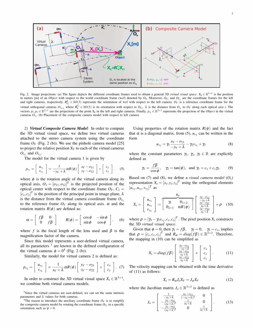
Fig. 3. Simulation Test 1: Large translational and rotational motion. (1) 3D robot end-effector trajectory in Cartesian (Xb); (2) image plane trajectories of6DVS, 2.5DVS, IBVS and PBVS (s); (3) feature errors in the image plane, (4) robot end-effector pose errors in 3D Cartesian space.
As shown in Fig. 3 (1), PBVS results in a straight line end-effector Cartesian trajectory. Since there is no control of theimage features, the image trajectory, (as shown in Fig. 3 (2)),is unpredictable and may leave the camera field of view. InIBVS, straight-line image trajectory is observed while the end-effector Cartesian trajectory is not controlled. For 2.5DVS, thetrajectory of the reference point in the image is a straight lineand the Cartesian trajectory is also well behaved. However,other points in image plane have curved trajectories.
Contrary to the previous approaches, the proposed 6DVShas a straight-line Cartesian trajectory (similar to that ofPBVS) and all the image features are “indirectly” controlled tomove approximately along straight-line trajectories like IBVS,see Fig. 3 (1), (2). Moreover, both the features errors and theCartesian pose errors converge to zero very smoothly withoutany overshooting (Fig. 3 (3), (4)). Although 2.5DVS has asimilar trade-off between these properties, the proposed 6DVSis more efficient and has better performance than 2.5DVS.Hence, 6DVS combines the advantages of PBVS in termsof controlling straight trajectories in Cartesian Space, and theadvantages of IBVS in terms of controlling image trajectories.
2) Test 2: For this test we compare the robustness of theproposed 6DVS, the classical IBVS and PBVS to cameraerrors. These errors are formulated as:
• Camera intrinsic parameter errors f = 1.1 f .• Camera extrinsic parameter errors T b
c = 1.1T bc .
The results from this test show that despite the cameraerrors, the controllers for each of the evaluated approachesdon’t become unstable. The resulting Cartesian and imagetrajectories have some notable differences (see Fig. 4), butare still well behaved.
Due to camera errors, the end-effector Cartesian trajectoryof PBVS deviates from the original straight-line trajectory toa circular motion, and slight effects on the image trajectoriescan also be observed (see Fig. 4 (c)). Slight differences inthe end-effector Cartesian trajectory of IBVS are shown inFig. 4 (b). As expected, the image trajectories for IBVS arerobust to camera errors. Fig. 4 (a) illustrates that the effects onboth Cartesian and image trajectories in the proposed 6DVSare minor. Hence, 6DVS is as robust to camera calibrationerrors as IBVS.
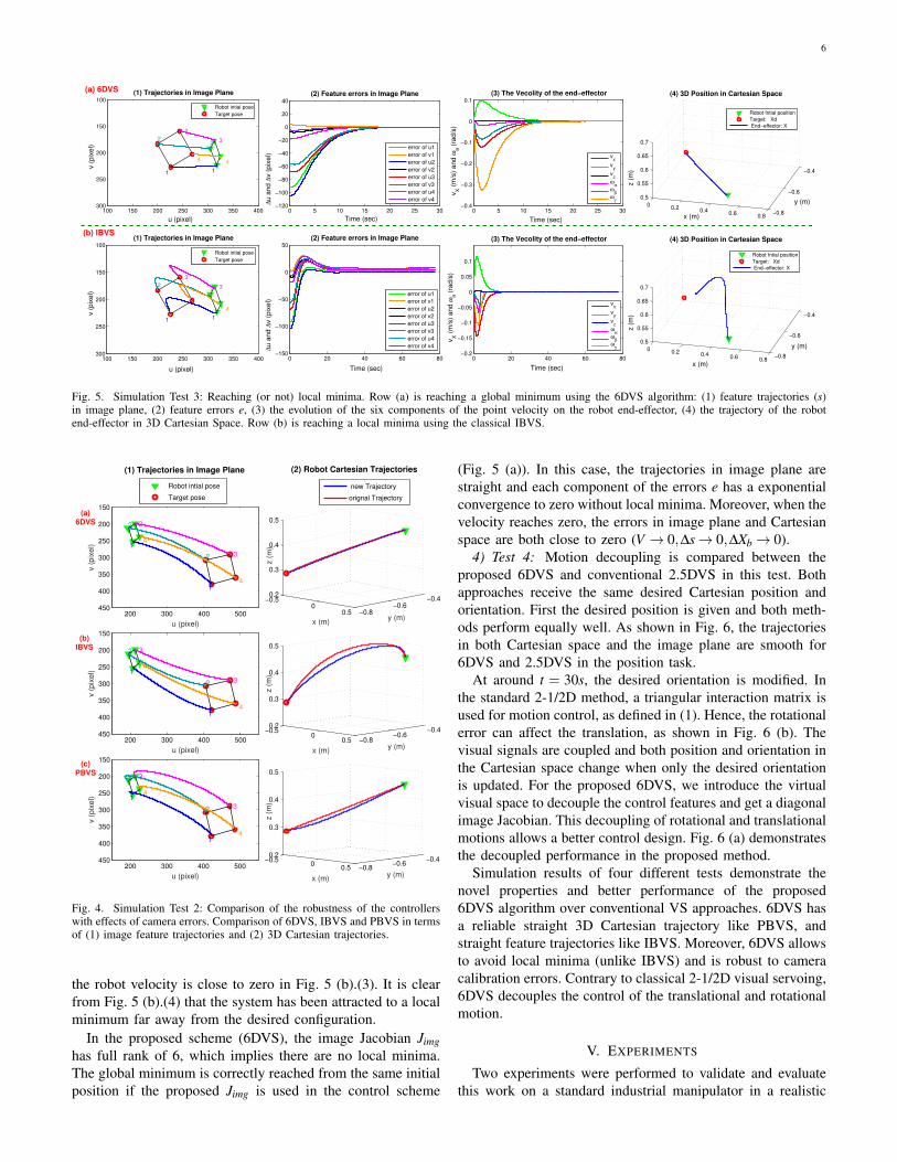
3) Test 3: In this test we evaluate a common problem inclassical IBVS: local minima. By definition, local minima arecases where V = 0 and s 6= sd . So, a local minimum is reachedwhen the point velocity on the robot end-effector is zero whileits final position is far away from the desired position. At thatposition, the errors s− sd in image plane do not completelyvanish (residual error is approximately two pixels on each uand v coordinate). Introducing noise in the image measurementleads to the same results.
Reaching such a local minimum is illustrated in Fig. 5 (b)for IBVS. Each component of the feature errors e has aexponential convergence but is not exactly zero (s 6= sd) while
6
100 150 200 250 300 350 400
100
150
200
250
300
11
2
3
4
2 3
4
u (pixel)
v (
pix
el)
(1) Trajectories in Image Plane
Robot intial pose
Target pose
0 5 10 15 20 25 30−120
−100
−80
−60
−40
−20
0
20
40
Time (sec)
∆u
an
d ∆
v (
pix
el)
(2) Feature errors in Image Plane
error of u1
error of v1
error of u2
error of v2
error of u3
error of v3
error of u4
error of v40
0.20.4
0.60.8
−0.8
−0.6
−0.4
0.5
0.55
0.6
0.65
0.7
y (m)
(4) 3D Position in Cartesian Space
x (m)
z (
m)
Robot Intial position
Target: Xd
End−effector: X
0 5 10 15 20 25 30−0.4
−0.3
−0.2
−0.1
0
0.1
Time (sec)
vX (
m/s
) a
nd
ωθ (
rad
/s)
(3) The Vecolity of the end−effector
vx
vy
vz
ωα
ωβ
ωγ
100 150 200 250 300 350 400
100
150
200
250
300
11
2
3
4
2 3
4
u (pixel)
v (
pix
el)
(1) Trajectories in Image Plane
Robot intial pose
Target pose
0 20 40 60 80−150
−100
−50
0
50
Time (sec)
∆u
an
d ∆
v (
pix
el)
(2) Feature errors in Image Plane
error of u1
error of v1
error of u2
error of v2
error of u3
error of v3
error of u4
error of v40 0.2 0.4 0.6 0.8
−0.8
−0.6
−0.4
0.5
0.55
0.6
0.65
0.7
y (m)
(4) 3D Position in Cartesian Space
x (m)
z (
m)
Robot Intial position
Target: Xd
End−effector: X
0 20 40 60 80−0.2
−0.15
−0.1
−0.05
0
0.05
0.1
Time (sec)
vX (
m/s
) a
nd
ωθ (
rad
/s)
(3) The Vecolity of the end−effector
vx
vy
vz
ωα
ωβ
ωγ
(b) IBVS
(a) 6DVS
Fig. 5. Simulation Test 3: Reaching (or not) local minima. Row (a) is reaching a global minimum using the 6DVS algorithm: (1) feature trajectories (s)in image plane, (2) feature errors e, (3) the evolution of the six components of the point velocity on the robot end-effector, (4) the trajectory of the robotend-effector in 3D Cartesian Space. Row (b) is reaching a local minima using the classical IBVS.
200 300 400 500
150
200
250
300
350
400
450
1
1
2 3
4
2 3
4
u (pixel)
v (
pix
el)
(1) Trajectories in Image Plane
Robot intial pose
Target pose
−0.50
0.5 −0.8−0.6
−0.40.2
0.3
0.4
0.5
y (m)
(2) Robot Cartesian Trajectories
x (m)
z (
m)
new Trajectory
orignal Trajectory
200 300 400 500
150
200
250
300
350
400
450
1
1
2 3
4
2 3
4
u (pixel)
v (
pix
el)
−0.50
0.5 −0.8−0.6
−0.40.2
0.3
0.4
0.5
y (m)x (m)
z (
m)
200 300 400 500
150
200
250
300
350
400
450
1
1
2 3
4
2 3
4
u (pixel)
v (
pix
el)
−0.50
0.5 −0.8−0.6
−0.40.2
0.3
0.4
0.5
y (m)x (m)
z (
m)
(b)IBVS
(c)PBVS
(a)6DVS
Fig. 4. Simulation Test 2: Comparison of the robustness of the controllerswith effects of camera errors. Comparison of 6DVS, IBVS and PBVS in termsof (1) image feature trajectories and (2) 3D Cartesian trajectories.
the robot velocity is close to zero in Fig. 5 (b).(3). It is clearfrom Fig. 5 (b).(4) that the system has been attracted to a localminimum far away from the desired configuration.
In the proposed scheme (6DVS), the image Jacobian Jimghas full rank of 6, which implies there are no local minima.The global minimum is correctly reached from the same initialposition if the proposed Jimg is used in the control scheme
(Fig. 5 (a)). In this case, the trajectories in image plane arestraight and each component of the errors e has a exponentialconvergence to zero without local minima. Moreover, when thevelocity reaches zero, the errors in image plane and Cartesianspace are both close to zero (V → 0,∆s→ 0,∆Xb→ 0).
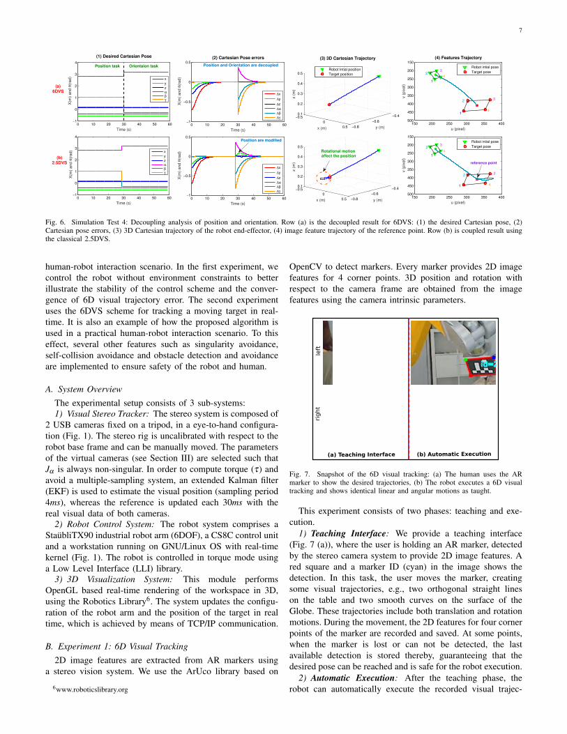
4) Test 4: Motion decoupling is compared between theproposed 6DVS and conventional 2.5DVS in this test. Bothapproaches receive the same desired Cartesian position andorientation. First the desired position is given and both meth-ods perform equally well. As shown in Fig. 6, the trajectoriesin both Cartesian space and the image plane are smooth for6DVS and 2.5DVS in the position task.
At around t = 30s, the desired orientation is modified. Inthe standard 2-1/2D method, a triangular interaction matrix isused for motion control, as defined in (1). Hence, the rotationalerror can affect the translation, as shown in Fig. 6 (b). Thevisual signals are coupled and both position and orientation inthe Cartesian space change when only the desired orientationis updated. For the proposed 6DVS, we introduce the virtualvisual space to decouple the control features and get a diagonalimage Jacobian. This decoupling of rotational and translationalmotions allows a better control design. Fig. 6 (a) demonstratesthe decoupled performance in the proposed method.
Simulation results of four different tests demonstrate thenovel properties and better performance of the proposed6DVS algorithm over conventional VS approaches. 6DVS hasa reliable straight 3D Cartesian trajectory like PBVS, andstraight feature trajectories like IBVS. Moreover, 6DVS allowsto avoid local minima (unlike IBVS) and is robust to cameracalibration errors. Contrary to classical 2-1/2D visual servoing,6DVS decouples the control of the translational and rotationalmotion.
V. EXPERIMENTS
Two experiments were performed to validate and evaluatethis work on a standard industrial manipulator in a realistic
7
0 10 20 30 40 50 60−1
0
1
2
3
4
Time (s)
X(m
) and θ
(rad)
x
y
zαβγ
0 10 20 30 40 50 60−1
−0.5
0
0.5
Time (s)
X(m
) and θ
(rad)
(2) Cartesian Pose errors
∆x
∆y
∆z
∆α∆β∆γ −0.5
0
0.5 −0.8
−0.6
−0.40.1
0.2
0.3
0.4
0.5
y (m)
(3) 3D Cartesian Trajectory
x (m)
z (
m)
Robot Intial position
Target position
150 200 250 300 350 400
150
200
250
300
350
400
450
500
1
1
23
4
23
4
u (pixel)
v (
pix
el)
(4) Features Trajectory
Robot intial pose
Target pose
0 10 20 30 40 50 60−1
0
1
2
3
4
Time (s)
X(m
) and θ
(rad)
x
y
zαβγ
0 10 20 30 40 50 60−1
−0.5
0
0.5
Time (s)
X(m
) and θ
(rad)
∆x
∆y
∆z
∆α∆β∆γ
−0.5
0
0.5 −0.8
−0.6
−0.40.1
0.2
0.3
0.4
0.5
y (m)x (m)
z (
m)
150 200 250 300 350 400
150
200
250
300
350
400
450
500
1
1
23
4
23
4
u (pixel)
v (
pix
el)
Robot intial pose
Target pose
Orientaion taskPosition task
(1) Desired Cartesian Pose
Position are modified
Position and Orientation are decoupled
reference point
Rotational motion affect the position(b)
2.5DVS
(a)6DVS
Fig. 6. Simulation Test 4: Decoupling analysis of position and orientation. Row (a) is the decoupled result for 6DVS: (1) the desired Cartesian pose, (2)Cartesian pose errors, (3) 3D Cartesian trajectory of the robot end-effector, (4) image feature trajectory of the reference point. Row (b) is coupled result usingthe classical 2.5DVS.
human-robot interaction scenario. In the first experiment, wecontrol the robot without environment constraints to betterillustrate the stability of the control scheme and the conver-gence of 6D visual trajectory error. The second experimentuses the 6DVS scheme for tracking a moving target in real-time. It is also an example of how the proposed algorithm isused in a practical human-robot interaction scenario. To thiseffect, several other features such as singularity avoidance,self-collision avoidance and obstacle detection and avoidanceare implemented to ensure safety of the robot and human.
A. System Overview
The experimental setup consists of 3 sub-systems:1) Visual Stereo Tracker: The stereo system is composed of
2 USB cameras fixed on a tripod, in a eye-to-hand configura-tion (Fig. 1). The stereo rig is uncalibrated with respect to therobot base frame and can be manually moved. The parametersof the virtual cameras (see Section III) are selected such thatJα is always non-singular. In order to compute torque (τ) andavoid a multiple-sampling system, an extended Kalman filter(EKF) is used to estimate the visual position (sampling period4ms), whereas the reference is updated each 30ms with thereal visual data of both cameras.
2) Robot Control System: The robot system comprises aStaubliTX90 industrial robot arm (6DOF), a CS8C control unitand a workstation running on GNU/Linux OS with real-timekernel (Fig. 1). The robot is controlled in torque mode usinga Low Level Interface (LLI) library.
3) 3D Visualization System: This module performsOpenGL based real-time rendering of the workspace in 3D,using the Robotics Library6. The system updates the configu-ration of the robot arm and the position of the target in realtime, which is achieved by means of TCP/IP communication.
B. Experiment 1: 6D Visual Tracking
2D image features are extracted from AR markers usinga stereo vision system. We use the ArUco library based on
6www.roboticslibrary.org
OpenCV to detect markers. Every marker provides 2D imagefeatures for 4 corner points. 3D position and rotation withrespect to the camera frame are obtained from the imagefeatures using the camera intrinsic parameters.
left
right
(a) Teaching Interface (b) Automatic Execution
Fig. 7. Snapshot of the 6D visual tracking: (a) The human uses the ARmarker to show the desired trajectories, (b) The robot executes a 6D visualtracking and shows identical linear and angular motions as taught.
This experiment consists of two phases: teaching and exe-cution.
1) Teaching Interface: We provide a teaching interface(Fig. 7 (a)), where the user is holding an AR marker, detectedby the stereo camera system to provide 2D image features. Ared square and a marker ID (cyan) in the image shows thedetection. In this task, the user moves the marker, creatingsome visual trajectories, e.g., two orthogonal straight lineson the table and two smooth curves on the surface of theGlobe. These trajectories include both translation and rotationmotions. During the movement, the 2D features for four cornerpoints of the marker are recorded and saved. At some points,when the marker is lost or can not be detected, the lastavailable detection is stored thereby, guaranteeing that thedesired pose can be reached and is safe for the robot execution.
2) Automatic Execution: After the teaching phase, therobot can automatically execute the recorded visual trajec-
8
300320
340360
380 −200
−100
0
10080
100
120
140
160
180
y (pixel)
(1) 3D Position in Virtual Visual Space
x (pixel)
z (
pix
el)
Target: Xsd
End−effector: Xs
−0.6−0.4
−0.20
0.2 −1
−0.5
0
0.4
0.5
0.6
0.7
0.8
y (m)
(2) 3D Position in Cartesian Space
x (m)
z (
m)
Target: Xd
End−effector: X
0 20 40 60 80 100 120 140−250
−200
−150
−100
−50
0
50
Time (sec)
Eu
ler
An
gle
s (
de
gre
e)
(3) 3D Orientation
αd
αβ
d
βγd
γ
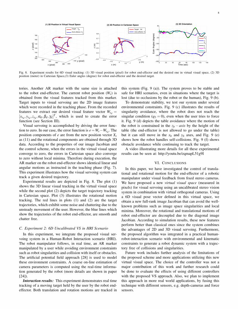
Fig. 8. Experiment results for 6D visual tracking: (1) 3D visual position (pixel) for robot end-effector and the desired one in virtual visual space, (2) 3Dposition (meter) in Cartesian Space,(3) Euler angles (degree) for robot end-effector and the desired target.
tories. Another AR marker with the same size is attachedto the robot end-effector. The current robot position (Ws) isobtained from the visual features tracked from this marker.Target inputs to visual servoing are the 2D image featureswhich were recorded in the teaching phase. From the recordedfeatures we extract our desired visual feature vector Wsd =[xsd ,ysd ,zsd ,αd ,βd ,γd ]
T , which is used to create the errorfunction (see Section III).
Visual servoing is accomplished by driving the error func-tion to zero. In our case, the error function is e=Ws−Wsd . Theposition components of e are from the new position vector Xsas (11) and the rotational components are obtained through 3Ddata. According to the properties of our image Jacobian andthe control scheme, when the errors in the virtual visual spaceconverge to zero, the errors in Cartesian space also convergeto zero without local minima. Therefore during execution, theAR marker on the robot end-effector shows identical linear andangular motions as instructed in the teaching phase (Fig. 7).This experiment illustrates how the visual servoing system cantrack a given desired trajectory.
Experimental results are depicted in Fig. 8. The plot (1)shows the 3D linear visual tracking in the virtual visual spacewhile the second plot (2) depicts the target trajectory trackingin Cartesian space. Plot (3) illustrates the rotational motiontracking. The red lines in plots (1) and (2) are the targettrajectories, which exhibit some noise and chattering due to theunsteady movement of the user. However, the blue lines whichshow the trajectories of the robot end-effector, are smooth andchatter free.
C. Experiment 2: 6D Uncalibrated VS in HRI Scenario
In this experiment, we integrate the proposed visual ser-voing system in a Human-Robot Interaction scenario (HRI).The robot manipulator follows, in real time, an AR markermanipulated by a user while avoiding environment constraintssuch as robot singularities and collision with itself or obstacles.The artificial potential field approach [28] is used to modelthese environment constraints. A coarse on-line estimation ofcamera parameters is computed using the real-time informa-tion generated by the robot (more details are shown in paper[24]).
Interaction results: This experiment demonstrates real timetracking of a moving target held by the user by the robot end-effector. Both translation and rotation motions are tracked in
this system (Fig. 9 (a)). The system proves to be stable andsafe for HRI scenarios, even in situations where the target islost (due to occlusions by the robot or the human), Fig. 9 (b).
To demonstrate stability, we test our system under severalenvironmental constraints. Fig. 9 (c) illustrates the results ofsingularity avoidance, where the robot does not reach thesingular condition (q3 = 0), even when the user tries to forceit. Fig. 9 (d) depicts the table avoidance where the motion ofthe robot is constrained in the zb− axis by the height of thetable (the end-effector is not allowed to go under the table)but it can still move in the xb and yb axes, and Fig. 9 (e)shows how the robot handles self-collisions. Fig. 9 (f) showsobstacle avoidance while continuing to track the target.
A video illustrating more details for all these experimentalresults can be seen at: http://youtu.be/zqmapL51g9I
VI. CONCLUSIONS
In this paper, we have investigated the control of transla-tional and rotational motion for the end-effector of a roboticmanipulator under visual feedback from fixed stereo cameras.We have proposed a new virtual visual space (measured inpixels) for visual servoing using an uncalibrated stereo visionsystem in combination with virtual orthogonal cameras. Usinga 6D visual pose vector defined in this virtual space, weobtain a new full-rank image Jacobian that can avoid the well-known problems such as image space singularities and localminima. Moreover, the rotational and translational motions ofrobot end-effector are decoupled due to the diagonal imageJacobian. According to simulation results, these new featuresperform better than classical ones since the system combinesthe advantages of 2D and 3D visual servoing. Furthermore,the proposed algorithm was integrated in a practical human-robot-interaction scenario with environmental and kinematicconstraints to generate a robot dynamic system with a trajec-tory free of collisions and singularities.
Future work includes further analysis of the limitations ofthe proposed scheme and more applications utilizing this newvirtual visual space. The choice of the controller was not amajor contribution of this work and further research couldbe done to evaluate the effects of using different controllerswith the proposed VS approach. Also, we plan to implementthis approach in more real world applications, by fusing thistechnique with different sensors, e.g. depth-cameras and forcesensors.
9
(a) (b) (c) (d) (e) (f)
Fig. 9. System behaviors: (a) Position and orientation tracking, (b) case when the target is lost, (c) case with singularity avoidance, (d) case with tablecollision avoidance, (e) case with self-collision avoidance and (f) obstacle avoidance.
REFERENCES
[1] S. Hutchinson, G. Hager, and P. Corke, “A tutorial on visual servocontrol,” IEEE Trans. Robot. Autom., vol. 12, no. 5, pp. 651–670, Oct.1996.
[2] J.-K. Oh, S. Lee, and C.-H. Lee, “Stereo vision based automation fora bin-picking solution,” Int. J. Control, Autom. Syst., vol. 10, no. 2, pp.362–373, 2012.
[3] B. Espiau, “Effect of camera calibration errors on visual servoing inrobotics,” in The 3rd Int. Symp. Experimental Robotics. London, UK:Springer-Verlag, 1993, pp. 182–192.
[4] F. Chaumette, “Potential problems of stability and convergence in image-based and position-based visual servoing,” in The Confluence of Visionand Control. LNCIS Series, No 237, Springer-Verlag, 1998, pp. 66–78.
[5] J. Wang and H. Cho, “Micropeg and hole alignment using imagemoments based visual servoing method,” IEEE Trans. Ind. Electron.,vol. 55, no. 3, pp. 1286–1294, Mar. 2008.
[6] F. Chaumette, “Image moments: a general and useful set of features forvisual servoing,” IEEE Trans. Robot., vol. 20, no. 4, pp. 713–723, Aug.2004.
[7] A. Krupa, J. Gangloff, M. de Mathelin, C. Doignon, G. Morel, L. Soler,J. Leroy, and J. Marescaux, “Autonomous retrieval and positioningof surgical instruments in robotized laparoscopic surgery using visualservoing and laser pointers,” in IEEE Int. Conf. Robot. Autom., vol. 4,May 2002, pp. 3769–3774.
[8] C. Collewet and F. Chaumette, “A contour approach for image-basedcontrol on objects with complex shape,” in IEEE/RSJ Int. Conf. Intell.Robots Syst., vol. 1, Nov. 2000, pp. 751–756.
[9] O. Tahri and F. Chaumette, “Point-based and region-based image mo-ments for visual servoing of planar objects,” IEEE Trans. Robot., vol. 21,no. 6, pp. 1116–1127, Dec. 2005.
[10] Y. Zhao, W.-F. Xie, and S. Liu, “Image-based visual servoing usingimproved image moments in 6-dof robot systems,” Int. J. Control,Autom. Syst., vol. 11, no. 3, pp. 586–596, 2013.
[11] J. Feddema, C. Lee, and O. Mitchell, “Model-based visual feedbackcontrol for a hand-eye coordinated robotic system,” Computer, vol. 25,no. 8, pp. 21–31, Aug. 1992.
[12] Y. Mezouar and F. Chaumette, “Optimal camera trajectory with image-based control.” Int. J. Robot. Res., vol. 22, no. 10, pp. 781–804, 2003.
[13] F. Chaumette and S. Hutchinson, “Visual servo control I: basic ap-proaches,” IEEE Robot. Autom. Mag., vol. 13, no. 4, pp. 82–90, Dec.2006.
[14] F. Janabi-Sharifi, L. Deng, and W. Wilson, “Comparison of basic visualservoing methods,” IEEE/ASME Trans. Mechatronics, vol. 16, no. 5, pp.967–983, Oct. 2011.
[15] N. Papanikolopoulos and P. Khosla, “Adaptive robotic visual tracking:theory and experiments,” IEEE Trans. Autom. Control, vol. 38, no. 3,pp. 429–445, Mar. 1993.
[16] E. Nematollahi and F. Janabi-Sharifi, “Generalizations to control lawsof image-based visual servoing,” Int. J. Optomechatronics, vol. 3, no. 3,pp. 167–186, 2009.
[17] D. Kim, A. Rizzi, G. Hager, and D. Zoditschek, “A robust convergentvisual servoing system,” in IEEE/RSJ Int. Conf. Intell. Robots Syst.,vol. 1, Aug. 1995, pp. 348–353.
[18] Y. Liu, H. Wang, C. Wang, and K. K. Lam, “Uncalibrated visual servoingof robots using a depth-independent interaction matrix,” IEEE Trans.Robot., vol. 22, no. 4, pp. 804–817, Aug. 2006.
[19] B. Yoshimi and P. Allen, “Alignment using an uncalibrated camerasystem,” IEEE Trans. Robot. Autom., vol. 11, no. 4, pp. 516–521, Aug.1995.
[20] K. Hosoda and M. Asada, “Versatile visual servoing without knowledgeof true jacobian,” in IEEE/RSJ Int. Conf. Intell. Robots Syst., vol. 1, Sep.1994, pp. 186–193.
[21] J. Piepmeier, G. McMurray, and H. Lipkin, “Uncalibrated dynamicvisual servoing,” IEEE Trans. Robot. Autom., vol. 20, no. 1, pp. 143–147, Feb. 2004.
[22] S. Azad, Farahmand, Amir-Massoud, and M. Jagersand, “Robust jaco-bian estimation for uncalibrated visual servoing,” in IEEE Int. Conf.Robot. Autom., May 2010, pp. 5564–5569.
[23] E. Malis, F. Chaumette, and S. Boudet, “2-1/2-D visual servoing,” IEEETrans. Robot. Autom., vol. 15, no. 2, pp. 238–250, Apr. 1999.
[24] C. Cai, E. Dean-Leon, N. Somani, and A. Knoll, “6d image-based visualservoing for robot manipulators with uncalibrated stereo cameras,” inIEEE/RSJ Int. Conf. Intell. Robots Syst., Sep. 2014.
[25] R. Hartley and A. Zisserman, Multiple View Geometry in ComputerVision (2. ed.). Cambridge University Press, 2004.
[26] M. W. Spong, S. Hutchinson, and M. Vidyasagar, Robot Dynamics andControl-Second Edition, 2004.
[27] C. Cai, E. Dean-Leon, D. Mendoza, N. Somani, and A. Knoll, “Un-calibrated 3d stereo image-based dynamic visual servoing for robotmanipulators,” in IEEE/RSJ Int. Conf. Intell. Robots Syst., Nov. 2013.
[28] C. Cai, N. Somani, S. Nair, D. Mendoza, and A. Knoll, “Uncalibratedstereo visual servoing for manipulators using virtual impedance control,”in Int. Conf. Control, Autom., Robot. Vision, Dec. 2014.


![Business cycles [Volume I] - Joseph Alois Schumpeter](https://static.fdocuments.in/doc/165x107/55cf8621550346484b9493ac/business-cycles-volume-i-joseph-alois-schumpeter.jpg)