CAD/FEA Tools and the Analysis of Design for Optimization
80
CAD/FEA TOOLS AND THE ANALYSIS OF DESIGN FOR OPTIMIZATION A Thesis Presented to The Faculty of the College of Science and Technology Morehead State University In Partial Fulfillment of the Requirements for the Degree Master of Science By Patil Yogesh October 21, 2006
Transcript of CAD/FEA Tools and the Analysis of Design for Optimization
CAD/FEA TOOLS AND THE ANALYSIS OF DESIGN FOR OPTIMIZATION
A Thesis
Presented to
The Faculty of the College of Science and Technology
Morehead State University
In Partial Fulfillment
of the Requirements for the Degree
Master of Science
By
Patil Yogesh
October 21, 2006

msu T}+E;sEs (bJD.OIY-l?.D:J~S -'yslf e-
Accepted by the faculty of the College of Science and Technology, Morehead State University, in partial fulfillment of the requirements for the Master of Science degree.
Master's Committee:
Date (

CAD/FEA TOOLS AND THE ANALYSIS OF DESIGN FOR OPTIMIZATION
Yogesh Patil, M.S. Morehead State University, 2006
Director of thesis: ~-d.,, f2. JO:..,..J '--'
This thesis is an experimental study of predicting an optimize #design of a
product using a simulation software. The main objective of this thesis is to emphasize
and explore the use of integrated computer aided design and finite element analysis
(CAD/FEA) software in O]Jtimizing the design and to reduce the physical testing
steps. To support this objective, a work-holding clamping plate (master design) is
designed on the Autodesk Inventor accompanied with the FEA package; the design is
then analyzed, using the stress analysis package (ANSYS) integrated with Inventor
version I 0. The design and the analysis results are then compared with the series of
modified designs of the master work-holding plate results. In the CAD/FEA
application tool, the model is constrained, loaded, and then the design is simulated for
stress analysis visualizing the magnitude of the stresses that occur throughout the part
and the deformation of the part, the stress factor of safety.
Accepted by:

INTRODUCTION
CONTENTS
CHAPTER I
General Area of Concern ................................................ 1
Objectives .................................................................. 2
Significance of the Study ..................................................... 2
Problem Statement ....................................................... 3
Layout ofThesis ........................................................ .4
Definition of Terms ..................................................... 5
CHAPTER II
REVIEW OF LITERATURE
Historical Overview .................................................... 8
Software Review ........................................................ 9
Finite Element Analysis Review .................................... .11
CHAPTER III
l\1ETHODOLOGY
General Description .................................................... 17
Basic Assumptions ...................................................... 17
Modeling of SPl ....................................................... .18
Model Formation ofSPl ....................................... 20
Model Analysis of SP 1 ......................................... 20
Modeling of SP2 ........................................................ 24
Model Formation of SP2 ....................................... 24
Model Analysis ofSP2 ......................................... 26

Modeling of SP3 ...................................................... 26
Model Formation of SP3 ..................................... 26
Model Analysis of SP3 ........................................ 28
Modeling of SP4 ...................................................... 30
Model Formation ofSP4 ..................................... 30
Model Analysis of SP4 ....................................... .31
Modeling of SP5 ...................................................... 33
Model Formation of SP5 ..................................... 33
Model Analysis of SP5 ....................................... .35
Modeling ofSP6 ...................................................... 37
Model Formation ofSP6 .................................... .37
Model Analysis ofSP6 ........................................ 39
CHAPTERIV
FINIDINGS AND CONCLUSION
General Remarks ..................................................... .41
Analysis Results of Solid Model SP 1 ............................. .41
Analysis Results of Solid Model SP2 ............................. .44
Analysis Results of Solid Model SP3 ............................. .48
Analysis Results of Solid Model SP4 .............................. 52
Analysis Results of Solid Model SP5 .............................. 56
Analysis Results of Solid Model SP6 .............................. 60
Mathematical Design ................................................. 63
Conclusion .............................................................. 73
References ..................................................................... 75

CHAPTER-I
INTRODUCTION
General Area of Concern
The trend of globalization has forced the manufacturing facilities to redesign
the manufacturing system to follow the steps of lean manufacturing and Just-In-Time
(JIT) production. The companies are trying to design the process technology and the
system to be flexible, controllable, and efficient. To be compatible with this
technological progress, it is relatively essential to emphasize the design and durability
of the product prior to sending the product to final production.
Basically, manufacturing is a value adding activity. and needs to be done in the
most efficient way, considering the least amount of time possible, optimum material
selection, and manpower. At the same time, it is necessary to have the right attributes
such as durability, light-weight, easy to maintain and cheaper product to remain
competitive. Design optimization is the only way to achieve this goal. Design
optimization is possible using design analysis tools. There are several finite element
analysis tools, independent or collaborative, can be used for predictable analysis of
the design for maximum allowable stress, maximum applied loads, breaking point of
the product, etc (Moaveni, S).
- 1 -
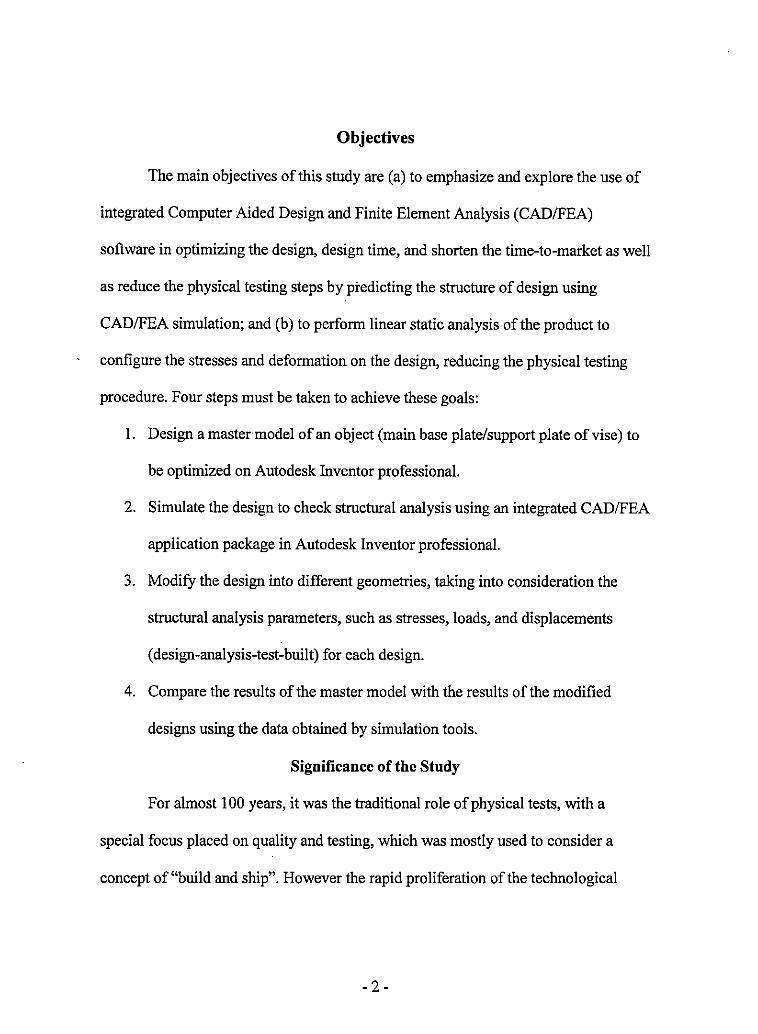
Objectives
The main objectives of this study are (a) to emphasize and explore the use of
integrated Computer Aided Design and Finite Element Analysis (CAD/FEA)
software in optimizing the design, design time, and shorten the time-to-market as well
as reduce the physical testing steps by predicting the structure of design using
CAD/FEA simulation; and (b) to perform linear static analysis of the product to
configure the stresses and deformation on the design, reducing the physical testing
procedure. Four steps must be taken to achieve these goals:
1. Design a master model of an object (main base plate/support plate of vise) to
be optimized on Autodesk Inventor professional.
2. Simulate the design to check structural analysis using an integrated CAD/FEA
application package in Autodesk Inventor professional.
3. Modify the design into different geometries, taking into consideration the
structural analysis parameters, such as stresses, loads, and displacements
(design-analysis-test-built) for each design.
4. Compare the results of the master model with the results of the modified
designs using the data obtained by simulation tools.
Significance of the Study
For almost 100 years, it was the traditional role of physical tests, with a
special focus placed on quality and testing, which was mostly used to consider a
concept of "build and ship". However the rapid proliferation of the technological
- 2 -

development in the last few years has changed the process of traditional physical
testing, adding into it the CAE tool and the finite element analysis tool. Design
analysis software helps to improve the product design, reduce material waste, save
time and get the product on the market faster than the competitors.
Inspired from the manufacturing revolution, industries are finding solutions to
minimize the overall costs of manufacturing and optimize the designs, in which the
design itself consumes 60% of the total cost. Design also includes physical testing
and analysis of the product.
The object of this study is to examine the feasibility of the integrated design
analysis CAD/FEA software application tool in optimizing the design of a support
plate for a vise taking into consideration the structural analysis parameters, such as
stress, displacements, and load. This simulation technique of design is used to predict
the real-world performance and the effect of design changes.
The study does not seek to develop a new and sophisticated analytical or
numerical model of a base plate, but to demonstrate the potentiality and the
effectiveness of the integrated CAD/FEA design analysis application tool to design an ·
optimized model of plate.
Problem Statement
The support plate is subjected to a distributed load horizontally on the
clamping face. The bottom of the plate is constrained to imitate the real-life situation
where the vise is tight fitted on a table with the help of nuts and bolts. The plate
design is determined using a designed load. The part geometry is modified in six
- 3 -

different designs, each design subjected to variation in load (1 0lbf, 20lbf, 30lbf,
40lbf, 50lbf, and 60lbf) to determine the geometric condition of the product. Plot the
deformed shape, and Von-Mises stress distribution from the results obtained, which
means, (a) Simulate the effect of material and geometric variations on the model due
to stresses; (b) Determine the displacement of the structure when the support plate is
subjected to known loads; and (c) Check the designed geometry for varying loads,
and redesign the model to ensure optimum results.
Layout of the Thesis
Chapter 2 "Review of Literature," presents the historical overview of the
integrated use ofCAD/FEA applications. The chapter involves some of the basic
terminology and concepts involved with CAD/CAM/FEA analysis. The chapter
gives a brief overview of manufacturing system, mastercam, CNC machine, ANSYS,
CAD/FEA software (AutoDesk Inventor 10). The chapter then goes into more
detailed information regarding the effective use of integrated CAD/FEA analysis.
Chapter 3 of this Thesis is entitled "Methodology." This chapter explains the
methodology used to obtain the goal. Several methods of lab work (such as designing
several clamping plate models, analyzing the design models and monitoring the
results) are discussed.
Chapter 4 of this Thesis js entitled "Findings." Which includes the
comparisons of the data collected using graphical representations to obtain the
proposed conclusion. The chapter also presents the future improvements to be made
in the usage of CAD/FEA.
-4-

Definition of Terms
1. CAE (Computer Aided Engineering)
CAE is a computer graphic simulation technology used to evaluate and
analyze the part geometry produced in CAD. CAE analysis includes two categories,
the finite element modeling and structural analysis, and mass property analysis.
2. CAD (Computer Aided Design)
CAD is a mechanical designing tool which uses a computer system to assist
the designer in creation, modification, analysis, or optimization of a design.
3. CAM (Computer Aided Manufacturing)
CAM is a form of automation where computers communicate work
instructions directly to the manufacturing machinery. CAM is a manufacturing tool
which is used to plan, manage, and control the operations of a manufacturing plant by
producing a tool-path of the CAD geometry and creating CNC (computer numerical
control) codes, either through direct or indirect computer interfacing.
4. Finite Element Analysis
The finite element analysis is a numeric modeling technique in which a
continuum is discretized into simple geometric shapes called elements. The elements
are joined together by shared nodes, an<;! the collection of nodes and elements are
called mesh (Rao, S).
( - 5 -
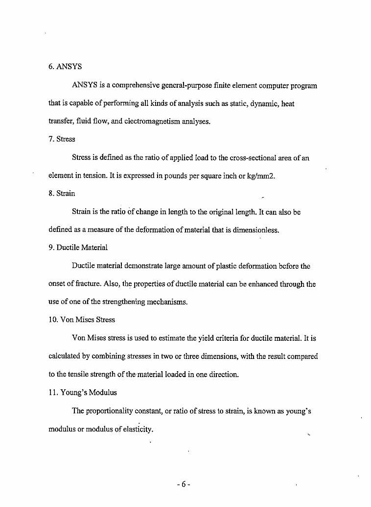
6.ANSYS
ANSYS is a comprehensive general-purpose finite element computer program
that is capable of performing all kinds of analysis such as static, dynamic, heat
transfer, fluid flow, and electromagnetism analyses.
7. Stress
Stress is defined as the ratio of applied load to the cross-sectional area of an
element in tension. It is expressed in pounds per square inch or kg/mm2.
8. Strain
Strain is the ratio of change in length to the original length. It can also be
defined as a measure of the deformation of material that is dimensionless.
9. Ductile Material
Ductile material demonstrate large amount of plastic deformation before the
onset of fracture. Also, the properties of ductile material can be enhanced through the
use of one of the strengthening mechanisms.
10. Von Mises Stress
Von Mises stress is used to estimate the yield criteria for ductile material. It is
calculated by combining stresses in two or three dimensions, with the result compared
to the tensile strength of the material loaded in one direction.
11. Young's Modulus
The proportionality constant, or ratio of stress to strain, is known as young' s
modulus or modulus of elasticity.
- 6 -

12. Poisson's Ratio
Poisson's ratio is the ratio of transverse contraction strain to longitudinal
extension strain in the direction of stretching forces.
13. CNC
The abbreviation CNC stands for computer numerical control, and refers to a
computer "controller" that reads G-code instructions and drives the machine tools, a
powered mechanical device typically used to fabricate metal components by the
selective removal of metal.
- 7 -

CHAPTER-II
REVIEW OF LITERATURE
Historical Overview
In the first quarter of the 20th century, a rigid mode of mass production
replaced batch-order production and job-order fabrication of products. There was a
massive increase in the household incomes in North America and Europe, followed
by the large-scale production of household appliances and motor vehicles. However,
product complexity and manufacturing inadaptability led to long product life cycles,
resulting in slow innovation and modifications. Then came the boom in international
manufacturing industries in post World War II in Western Europe, U.S.A., and Japan.
These global industries competed for their respective market shares with the domestic
companies within these countries. Due to globalization, the industries reconstructed
their prior-to-manufacturing techniques, emphasizing the design to obtain a quality
product that would be competitive, aesthetically and ergonomically. The engineering
design starts with the customer's viewpoint or feedback or in response to an idea
developed by research team, initiated on the CAD (Benhabib, B).
Before creating a solid geometric model, there are several factors that need to
be considered:
1. Create optimum or optimize product architecture and conceptual product
design.
2. Pursue off-the-shelf and modularity opportunities.
- 8 -

3. Allocate an appropriate material selection.
4. Understand the potential processes that will manufacture the parts.
5. Design for efficient manufacturing, considering the total cost.
6. Correct dimensioning and tolerance consideration (Anderson, D).
Software Review
CAD (Computer Aided Design)
Introduced in the 1960s, CAD tools are the most common geometric modeling
tools with advanced improvement of designing 3D modeling. Geometric modeling is
the first step in CAE (Computer-Aided Engineering) analysis of a design. The
objective is to encapsulate all geometric data pertaining to the part in a single model
and specify all necessary material properties as additional information. Solid
modeling, as a branch of geometric modeling, refers to the geometric description of
solid objects in their entirety (Groover, P., Zimmers, W).
Autodesk Inventor
Autodesk Inventor, in this thesis, is a CAD software used to design a solid
model (support plate for a vise). Autodesk Inventor also includes an advanced feature
of third-party analysis tool ANSYS, a finite element analysis tool, to analyze the
design for stresses and deformations. Autodesk Inventor a is mechanical design
software which includes assembly-centric solid modeling and drawing production
systems, tools, and commands to complete fully parametric three-dimensional parts,
assemblies, and presentations, and two-dimensional drawings. Autodesk Inventor
provides a combination of industry-specific tools that extend the capabilities of solid
- 9 -

modeling techniques for completing complex machinery and other product designs.
Figure I shows the Autodesk Inventor interface (Madsen, P).
□Twopohl:~ •
°'lfi< • e Poilt:, Mu Cerur
0-lllHrto~P«tem l)Ci-oJi,,P~n i@Offsi:t
-0Geneorlll0mensicn D ..---
Figure I. Autodesk Inventor Professional Environnent.
The term "interface" used here is to describe the tools and techniques used to provide
and receive information to and from a computer program. The interface window
includes the following:
Menu system bar
The menu system interface has several groups of pull-down menu features
which provide the text-based, menu configuration. A designer can pick any of these
- 10 -

pull-down menus to reveal the options for that menu, and move the cursor down and
up to highlight any of the options.
Panel bar
The panel bar provides the list of several design tools available for creating
models in a specific work environment where we are currently working. For example,
when working on 2D drawing or sketch mode, only sketching tools are available;
when moved to finish sketch, then the features menu becomes available.
Browser bar
The browser stores and displays all the objects in the model. The design can
be modified using the right-click on the processes done on the model, using the edit
mode.
Toolbars
Toolbars and toolbar icons are used to perform specific tasks which help in
modifying the model. Some of the features of tool bars are rotate, zoom to fit, pan,
zoom area, etc.
Command bar
Command bar is one of the important tools used in Autodesk Inventor, which
contains select, sketch, update, and color or style drop down lists.
Finite Element Analysis Review
The finite element analysis tool in this thesis is a tool to understand better how
a design will perform under certain conditions. Here the stress analysis tool is a third
party application tool supported by ANSYS. Autodesk Inventor Professional stress
- 11 -

analysis provides tools for determining structural design performance directly on the
Autodesk Inventor model. The stress analysis includes tools to place loads and
constraints on a part and calculate the resulting stress, deformation, safety factor, and
resonant frequency modes. A completely virtual product development system saves
money and moves products to market faster (Madsen, P). Figure 2 shows the AIP
stress analysis environment.
:Boo ~ ~ ir-t Fginet ioo1s t.Oll>'flt ~ !£f'dow WfQ t1't1 i (ii illf + .,,,.J~.l~J i_Q __ ': ___ fS_JalJ_~ (°" i!~Select
.; .. ~ # ...... );.{BeM"Qload ..,_ ~8ooft.fuds,
,i:fuedcon:sb...t
0:,llt!CO"Wlllrt
~f'n'lltoffl Constr...-t
"""'" 'll"eort u-m5tren~~
A Expgrt to IW5YS
Figure 2. Stress Analysis Environment.
The design phase is the key phase of a manufacturing system, so it is of prime
significance to perform an analysis of a mechanical part designed in the design phase
to bring a better product to market in less time. The analysis of design helps
determine if the part is strong enough to withstand expected loads or vibrations
- 12 -
without breaking or deforming inappropriately (Hryniewieki, J). AIP stress analysis
also helps in gaining valuable insight at an early stage when the cost of redesign is
smal1 and helps in predicting whether the part can be redesigned in a more cost
effective manner and still performs satisfactorily under expected use. Autodesk
Inventor professional stress analysis environment consists of the following menus:
Stress analysis environment
The stress analysis environment enables the designer to simulate the part's
behavior under externally imposed loads and frequencies. The Stress Analysis Update
tool then performs an analysis to evaluate the performance of the part in response to
the applied force and constraints.
The stress analysis panel bar
The stress analysis panel bar includes stress analysis tools briefly described
below:
Force
The force tool is used to apply forces of the selected magnitude on the
selected faces, edges, or vertices, to analyze the behavior of the design under the
applied force.
Pressure
The pressure tool is used to apply forces of the selected magnitude on the
selected faces to analyze the behavior of the design under the applied pressure.
- 13 -

Bearing load
The bearing load tool is used to apply bearing load of the selected magnitude
on the selected cylindrical faces to analyze the behavior of the design under the
applied bearing load.
Moment
The moment tool is used to apply the moment of selected magnitude on the
selected'faces to analyze the behavior of the design under the applied moment of
inertia.
Body loads
The body load tool is used to apply the moment of selected magnitude on the
part to analyze the behavior of the design under the applied body load.
Fixed constraint
·Toe fixed constraint tool is used to place a fixed constraint on any of the faces,
edges, or vertices defined in the part. To apply a fixed constraint you must first select
a valid material and enter the stress analysis environment.
Pin constraints
Pin constraint tool is used to apply pin constraint of the selected combination
on cylindrical and curved faces.
Frictionless constraint
The frictionless constraint tool is used to apply frictionless constraint on faces. )
Frictionless constraint prevents the surface from moving or deforming in the normal
- 14 -
direction relative to the surface. The surface is free to rotate, move, or deform in
tangential direction to the applied frictionless constraint.
Stress analysis update
Stress analysis update is used to make change to the part, or stress analysis
settings after the part is analyzed. Use the Stress Analysis Update tool to run a new
analysis on the part. The tool analyzes the part considering the changes made and
generates a valid solution.
Report
The Stress Analysis Report documents the design and analysis information
created. It is divided into sections that correspond to objects in the browser. Each
scenario in the report represents one complete engineering simulation. The definition
of a simulation includes known factors about a design such as material properties of
the part, and types and magnitudes ofloads and constraints.
Animate results
Using the Animate Results tool, you can visualize the part through various
stages of deformation. The designer can also animate stress, safety factor, and
deformation under frequencies.
Stress analysis setting
Using Stress Analysis Settings on the stress analysis panel bar, you can
modify the mesh fineness on the scale of -100 to I 00. The element size is determined.
based on the size of the body box, the proximity of other topologies, body curvature,
and the complexity of the feature.
- 15 -

Export.to ANSYS
The Export to ANSYS tool is used to create a copy of the analysis file which
is compatible with ANSYS Workbench. The file is stored with a .dsdb extension.
Stress analysis browser
The stress analysis browser displays all the defined loads and constraints,
input conditions, and results of the part. Loads and constraints !ll"e placed at the top of
the hierarchy after the origin folder, and before all other folders. You can also view
the type of material selected for the analysis.
- 16 -

CHAPTER - III
METHODOLOGY
General Description
This chapter discusses the design and analysis of a vise base plate which
undergoes deformation due to the forces applied when clamping the parts.
The vise was assumed to be modeled with the material properties of cast iron. It was
also assumed that the cast iron used in this product has isotropic properties. An
Isotropic material implies that the material properties do not vary with direction. The
elastic properties of an Isotropic material are fully defined by a single value of
Young's Modulus and a single value of Poisson's Ratio (Black, J., DeGarmo, Kohser,
E., Ronald A). The controlled model shown in Figure 4 (page 20) was a variation of a
model ( a replica of the support plate as shown in Figure 3 on page 19) with the
statistics as shown in Table 1 (page 18). The test models were modifications and
improvements from the control model. The models were built and analyzed using an
integrated CAD/FEA Software from Autodesk inventor 10. These models have the
same length but different geometries; the change in geometries is the result of the
improvement analysis.
Basic Assumptions
For the purpose of this thesis, several assumptions were made to simplify the analysis
of the model. These_ basic assumptions are:
- 17 -
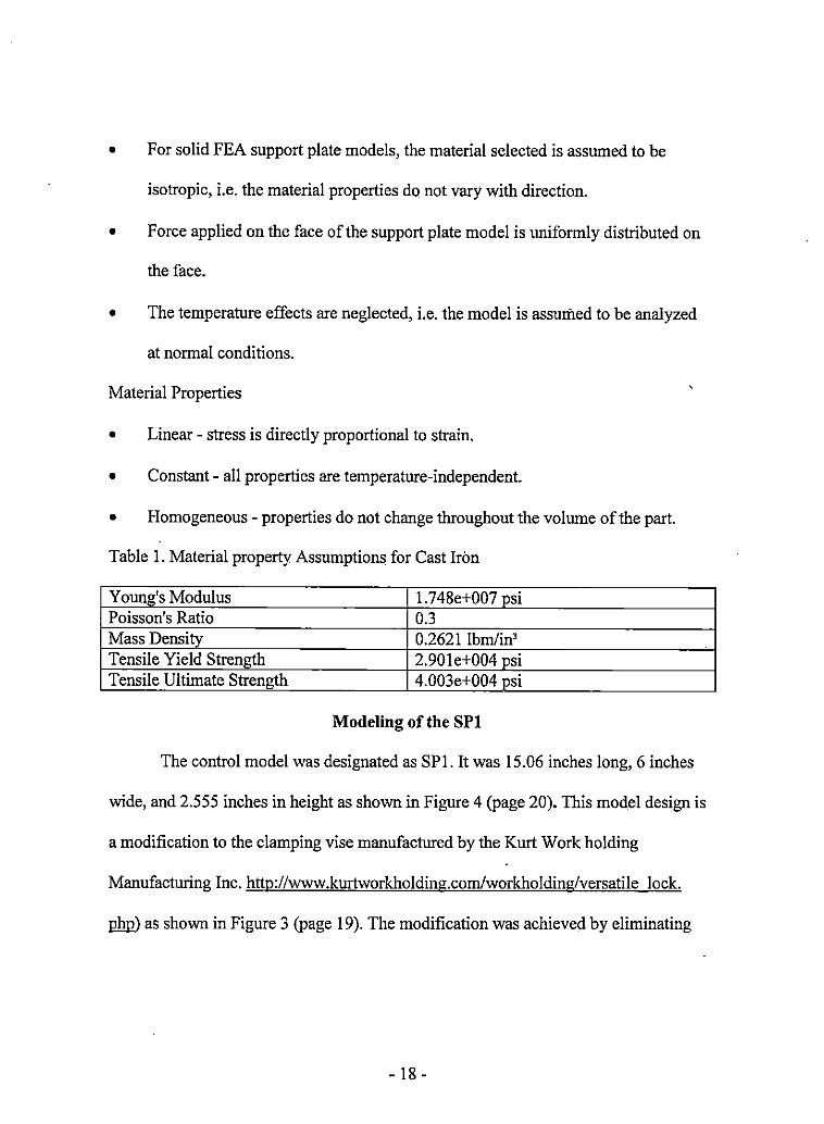
• For solid FEA support plate models, the material selected is assumed to be
isotropic, i.e. the material properties do not vary with direction.
• Force applied on the face of the support plate model is uniformly distributed on
the face.
• The temperature effects are neglected, i.e. the model is assumed to be analyzed
at normal conditions.
Material Properties
• Linear - stress is directly proportional to strain.
• Constant - all properties are temperature-independent.
• Homogeneous - properties do not change throughout the volume of the part.
Table 1. Material property Assumptions for Cast Iron
Young's Modulus 1. 7 48e+007 osi Poisson's Ratio 0.3 Mass Density 0.2621 lbm/in' Tensile Yield Stremrth 2.901e+004 osi Tensile Ultimate Strength 4.003e+004 psi
Modeling of the SPl
The control model was designated as SPl. It was 15.06 inches long, 6 inches
wide, and 2.555 inches in height as shown in Figure 4 (page 20). This model design is
a modification to the clamping vise manufactured by the Kurt Work holding
Manufacturing Inc. http://www.kurtworkholding.com/workholding/versatile lock.
p1m) as shown in Figure 3 (page 19). The modification was achieved by eliminating
- 18 -
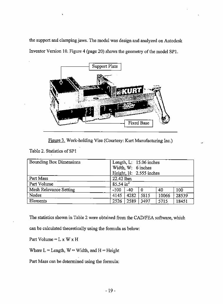
the support and clamping.jaws. The model was design and analyzed on Autodesk
Inventor Version 10. Figure 4 (page 20) shows the geometry of the model SPl.
Support Plate
Fixed Base
Figure 3. Work-holding Vise (Courtesy: Kurt Manufacturing Inc.)
Table 2. Statistics of SP!
Bounding Box Dimensions Length, L: 15. 06 inches Width, W: 6 inches Height, H: 2.555 inches
Part Mass 22.42 lbm Part Volume 85.54 in" Mesh Relevance Setting -100 -40 0 40 Nodes 4145 4282 5815 10066 Elements 2526 2589 3497 5715
100 28539 18451
The statistics shown in Table 2 were obtained from the CAD/FEA software, which
can be calculated theoretically using the formula as below:
Part Volume= L x Wx H
Where L = Length, W = Width, and H = Height
Part Mass can be determined using the formula:
- 19 -
Density= Mass/ Volume
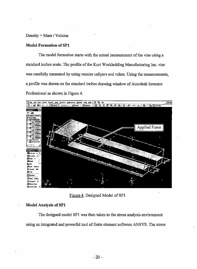
Model Formation of SPl
The model formation starts with the actual measurement of the vise using a
standard inches scale. The profile of the Kurt Workholding Manufacturing Inc. vise
was carefully measured by using vernier calipers and rulers. Using the measurements,
a profile was drawn on the standard inches drawing window of Autodesk Inventor
Professional as shown in Figure 4 .
... Wiii 1z4 (9~ E ·A @~11.[ ~1101o"1 ,' ..,._. I
Q;:,,Rt> k.,
6illcft Shtt+I
g,,..,, "" ;;;,.
'3>- -~d>o,nlo,, st
l'.lj-F-. t:ill,F,,uDraft ;•::-::
Model Analysis of SPl
Figure 4. Designed Model ofSPl
The designed model SPl was then taken to the stress analysis environment
using an integrated and powerful tool of finite element software ANSYS. The stress
- 20-
analysis environment was made active using just one click of the mouse. The panel
bar changes from part feature tools to stress analysis tools.
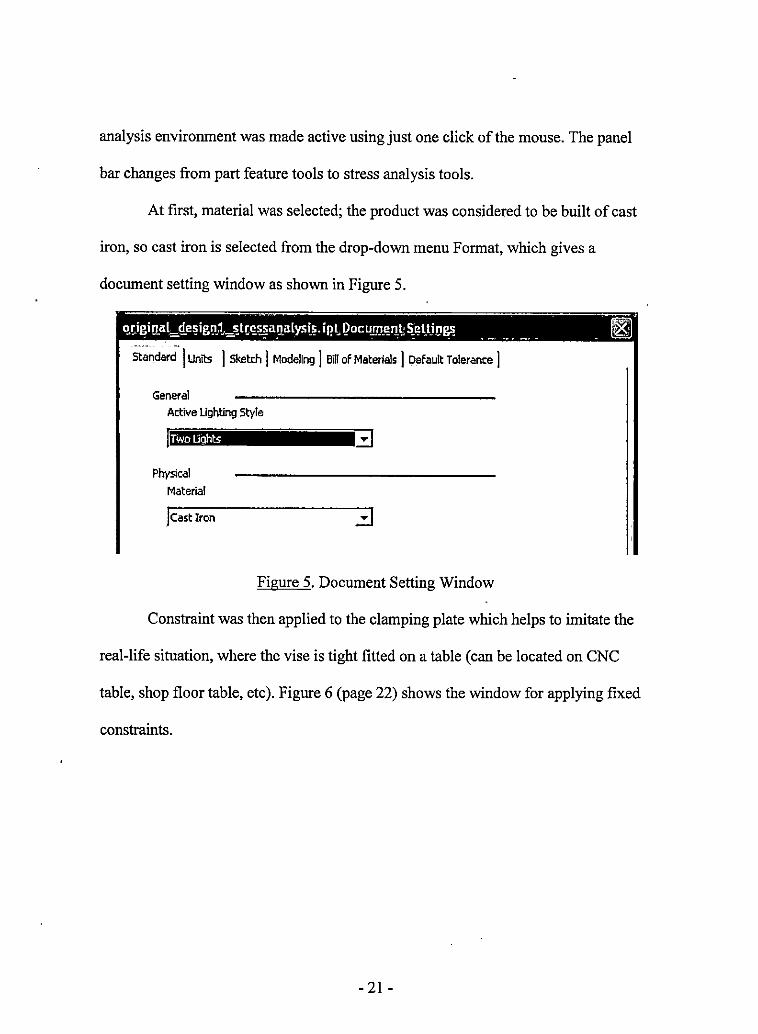
At first, material was selected; the product was considered to be built of cast
iron, so cast iron is selected from the drop-down menu Format, which gives a
document setting window as shown in Figure 5.
St~ndard-j Units I Sketch ] Modeling I Bill of Materials I Default Tolerance ]
General Active Lighting Style
Physical
Material
]cast Iron
Figure 5. Document Setting Window
Constraint was then applied to the clamping plate which helps to imitate the
real-life situation, where the vise is tight fitted on a table (can be located on CNC
table, shop floor table, etc). Figure 6 (page 22) shows the window for applying fixed
constraints.
- 21 -
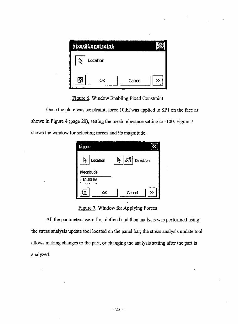
1 ~ Location
@ j __ o_K_....J __ ca_n_ce_l --JI GJ Figure 6. Window Enabling Fixed Constraint
Once the plate was constraint, force l0lbfwas applied to SPl on the face as
shown in Figure 4 (page 20), setting the mesh relevance setting to -100. Figure 7
shows the window for selecting forces and its magnitude.
~ Location
Magnitude
OK
~ .J<S I Direction
Cancel j ~~-I Figure 7. Window for Applying Forces
All the parameters were first defined and then analysis was performed using
the stress analysis update tool located on the panel bar; the stress analysis update tool
allows making changes to the part, or changing the analysis setting after the part is
analyzed.
-22-
Analysis Type
Mesh Control-------
Mesh Relevance
I I I I I • I I I
-100 O 100
r R<=it Convergence
Preview Mesh
OK Cancel
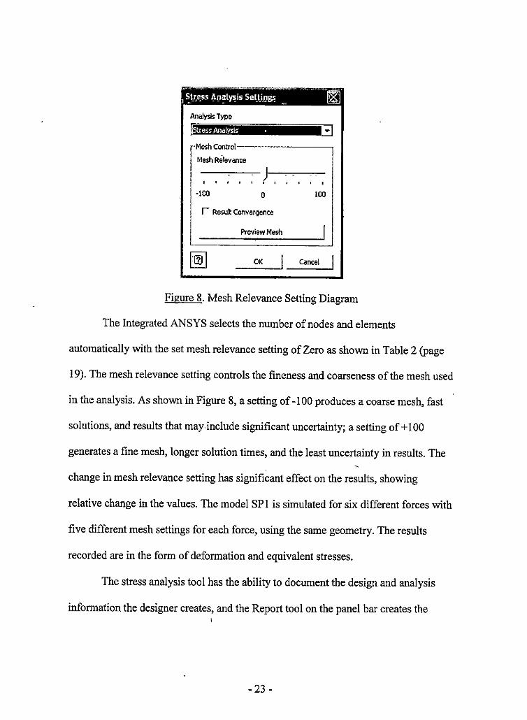
Figure 8. Mesh Relevance Setting Diagram
The Integrated ANSYS selects the number of nodes and elements
automatically with the set mesh relevance setting of Zero as shown in Table 2 (page
19). The mesh relevance setting controls the fineness and coarseness of the mesh used
in the analysis. As shown in Figure 8, a setting of -100 produces a coarse mesh, fast
solutions, and results that may include significant uncertainty; a setting of+ 100
generates a fine mesh, longer solution times, and the least uncertainty in results. The
change in mesh relevance setting has significant effect on the results, showing
relative change in the values. The model SP 1 is simulated for six different forces with
five different mesh settings for each force, using the same geometry. The results
recorded are in the form of deformation and equivalent stresses.
The stress analysis tool has the ability to document the design and analysis
information the designer creates, and the Report tool on the panel bar creates the
-23 -
document in HTML format. The report also shows the diagram of deformation
caused, due to the load on the SP I.
Modeling of the SP2
Model Formation of SP2
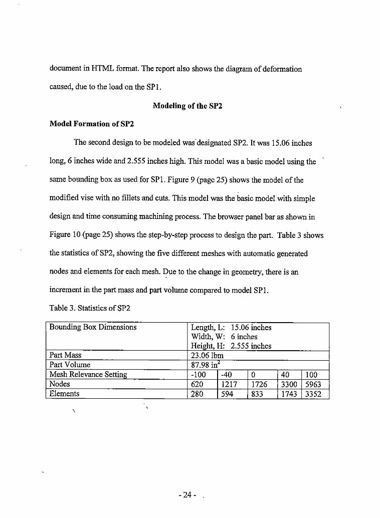
The second design to be modeled was.designated SP2. It was 15.06 inches
long, 6 inches wide and 2.555 inches high. This model was a basic model using the
same bounding box as used for SP!. Figure 9 (page 25) shows the model of the
modified vise with no fillets and cuts. This model was the basic model with simple
design and time consuming machining process. The browser panel bar as shown in
Figure 10 (page 25) shows the step-by-step process to design the part. Table 3 shows
the statistics of SP2, showing the five different meshes with automatic generated
nodes and elements for each mesh. Due to the change in geometry, there is an
increment in the part mass and part volume compared to model SP 1.
Table 3. Statistics of SP2
Bounding Box Dimensions Length, L: 15.06 inches Width, W: 6 inches Height, H: 2.555 inches
Part Mass 23.06 lbm Part Volume 87.98 in" Mesh Relevance Setting -100 -40 0 40 100 Nodes 620 1217 1726 3300 5963 Elements 280 594 833 1743 3352
-24- .

Figure 9. Designed Model of SP2
-'W I .Ii\ Gil origlnal_designl _stressanalysis. ipt + L)Origin - IElJ Extrusion!
~Sketch! Extrusion2 ·
~Sketch2 IElJ Extrusion3 ~Sketch3
Extrusion4 ~Sketch4
Extrusions ~Sketch5
@l Chamfer! End of Part
Figure 10. Solid Modeling Steps
- 25 -

Model Analysis of SP2
The FEA mesh for SP2 was regenerated from the method described under the
model analysis of SP 1. Material Selection is the first step in the model analysis to
assign the part with the material properties as shown in Table 1 (page 18). The model
SP2 was considered to be built with cast iron. Then the stress analysis setting tool
shown in Figure 8 (page 23) is made active to select the required mesh from coarser
to finer. The methodology uses five different meshes of -100, -40, 0, 40, and I 00.
Then constraint was applied at the bottom of the SP2 with the default zero load
setting holding the vise to a fixed position. Load l0lbfis applied on the face of the
clamp as shown in Figure 9 (page 25). Once the parameters are set the Stress Analysis
Update tool was selected to start the analys\s. After obtaining the result for 1 0lbf
force, mesh -100, the model was analyzed for mesh -40, similarly for mesh 0, mesh
40 and mesh 100. Then force 20lbf, 30lbf, 40lbf, 50lbf, and 60lbf are applied to SP2
for five different meshes. The results indicating deformations and equivalent stresses
are gathered and recorded in ascending order as shown in Table 9 (page 45).
Modeling of SP3
Model Formation of SP3
The design model 3 was designated as SP3. SP3 was modified using the same
bounding box, but with a slight change in the geometry, increasing the part mass. The
modification of SP3 was random modification with the result unknown. Figure 11
(page 27) shows'the solid model of SP3. The model formation steps are as shown in
Figure 12 (page 28) which includes the time consuming model formation features.
-26-

Table 4 lists the statistics of SP3 showing the five different meshes with automatic
generated nodes and elements for each mesh. Due to the change in geometry, there is
a small change in the part mass and part volume.
Table 4.,Statistics of SP3
Bounding Box Dimensions Length, L: 15.06 inches Width, W: 6 inches Height, H: 2.555 inches
Part Mass 22.71 lbm Part Volume 86.63 in' Mesh Relevance Setting -100 -40 0 40 100 Nodes 687 1376 1971 3842 6532 Elements 315 686 989 2127 3738
Figure 11. Designed Model of SP3
-27 -

Model Analysis of SP3
·on2
Sketch2 Extruslon3
Sketch3 mferl
trusion4 « Sketch'! Extruslon5
, SketchS @ End of Part
Figure 12. Solid Model Steps
The FEA mesh for SP3 was regenerated from the method described under the
model analysis of SP 1. The first step to be considered in the model analysis is to
select material and assign the part with the material properties as shown in Table 1
(page 18). The model SP3 was considered to be built with cast iron. The stress
analysis setting tool shown in Figure 14 (page 29) is made active to-select the
required mesh from coarser to finer. The methodology uses five different meshes of -
100, -40, 0, 40, and 100. The constraint is applied at the bottom of the model SP3
with the default zero load setting, holding the vise to a fixed position. Figure 13 (page
29) shows the fixed constraints tool activated, enabling the designer to apply
constraints on the highlighted face of SP3.
- 28 -

Figure 13. Shows Fixed Constraints Application.
Load 1 0lbf was applied on the face of the clamp as shown in Figure 11 (page
27). Then the mesh relevance setting was adjusted on -100 as shown in Figure 14,
which makes the mesh coarser. Once the parameters are set the Stress Analysis
Update tool was selected to start the analysis.
~;~~~ .,oo ~I rr_ .. _..i:~c_-_.,_ .. _"'_' __ ~ I
Preview Mesh J i
Figure 14. Stress Analysis Setting
- 29-
After obtaining the result for 1 Olbf force, mesh -100 the model was analyzed
for mesh -40, similarly for mesh 0, mesh 40 and mesh 100. Then force 20lbf, 30lbf,
40lbf, 50lbf, and 60lbf are applied to SP3 for five different meshes. The results in the
form of deformations and equivalent stresses are gathered and recorded in ascending
order as shown in Table 10 (page 49).
Modeling of SP4
Model Formation of SP4
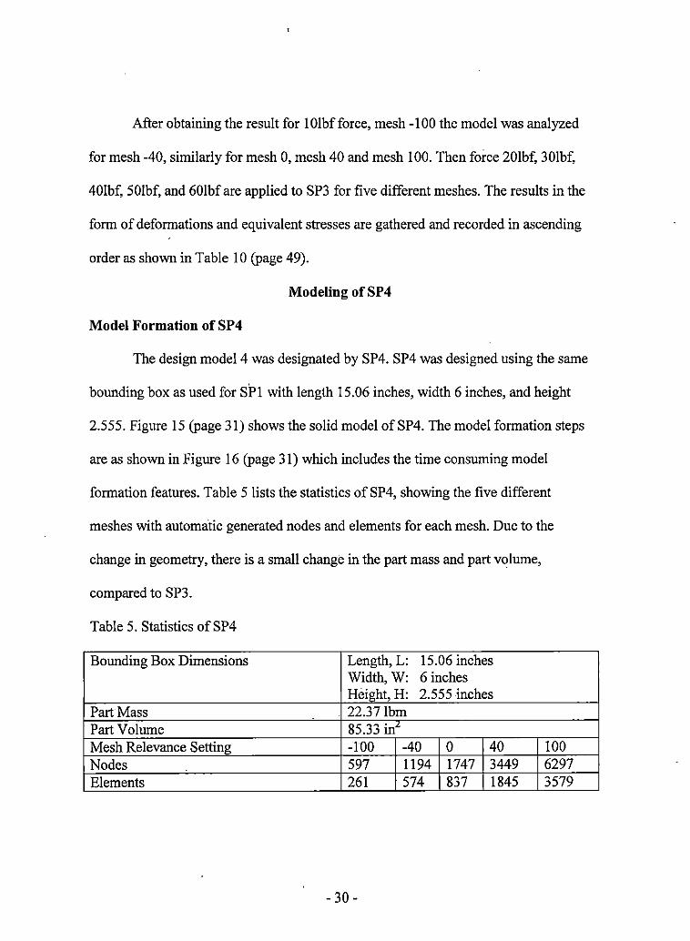
The design model 4 was designated by SP4. SP4 was designed using the same
bounding box as used for SPl with length 15.06 inches, width 6 inches, and height
2.555. Figure 15 (page 31) shows the solid model ofSP4. The model formation steps
are as shown in Figure 16 (page 31) which includes the time consuming model
formation features. Table 5 lists the statistics of SP4, showing the five different
meshes with automatic generated nodes and elements for each mesh. Due to the
change in geometry, there is a small change in the part mass and part volume,
compared to SP3.
Table 5. Statistics ofSP4
Bounding Box Dimensions Length, L: 15.06 inches Width, W: 6 inches Height, H: 2.555 inches
Part Mass 22.37 lbm Part Volume 85.33 in"' Mesh Relevance Setting -100 -40 0 40 100 Nodes - 597 1194 1747 3449 6297 Elements 261 574 837 1845 3579
- 30 -

Figure 15. Design Model ofSP4
Extrusion! Sketch!
Extrusion2 , Sketch2
Chamfer! Extrusion6
Sketch6 Extrusion? • Sketch?
Extrusions Sketcha
End of Part
Figure 16. Solid Modeling Steps
Model Analysis of SP4
The FEA mesh for SP4 was regenerated from the method described under
model analysis of SP!. Material Selection is the first step in the model analysis to
assign the part with the material properties as shown in Table I (page 18). The model
- 31 -

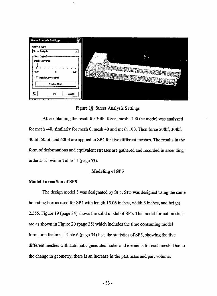
SP4 was considered to be built with cast iron. Then the stress analysis setting tool
shown in Figure 18 (page 33) was made active to select the required mesh from
coarser to finer. The methodology uses five different meshes of -100, -40, 0, 40, and
100. Then constraint was applied at the bottom of the SP4, with the default zero load ·
setting holding the vise to fixed position. Figure 17 shows the fixed constraints tool
activated, enabling the designer to apply constraints on the highlighted face of SP4.
Figure 17. Fixed Constraint Application
Load lOlbf is applied on the face of the clamp as shown in Figure 15. Then ·
the mesh relevance setting was adjusted on -100 as shown in Figure 18 (page 33), .
which makes the mesh coarser. Once the parameters are set, the Stress Analysis
Update tool is selected to start the analysis.
- 32 -
-Type ,,.,.,, Anoly,is
MeshControl------Mesh Relevance
·100 D
r Resutt Convetva,ce --OK
Figure 18. Stress Analysis Settings
After obtaining the result for 1 0lbf force, mesh -100 the model was analyzed
for mesh -40, similarly for mesh 0, mesh 40 and mesh 100. Then force 20lbf, 30lbf,
40lbf, 50lbf, and 60lbf are applied to SP4 for five different meshes. The results in the
form of deformations and equivalent stresses are gathered and recorded in ascending
order as shown in Table 11 (page 53).
Modeling of SPS
Model Formation of SPS
The design model 5 was designated by SP5. SP5 was designed using the same
bounding box as used for SPl with length 15.06 inches, width 6 inches, and height
2.555. Figure 19 (page 34) shows the solid model ofSP5. The model formation steps
are as shown in Figure 20 (page 35) which includes the time consuming model
formation features. Table 6 (page 34) lists the statistics of SP5, showing the five
different meshes with automatic generated nodes and elements for each mesh. Due to
the change in geometry, there is an increase in the part mass and part volume.
- 33 -

Table 6. Statistics of SP5
Bounding Box Dimensions
Part Mass Part Volume Mesh Relevance Setting Nodes Elements
----·"".J.)I
JrnttHIW ~El<tr>.de E ~ (mR~ R {'1
~Hale H 1~:• lfjl9ie1 '.,_1) tl,Rb Lb
6itdt Shfl;~
!lo,_, ..
"'"' &Fikt, Shit.f tJ'lo-n,, Slej:M:,-,.,,Fac,,,
~~-~-~-_ffj
Length, L: 15.06 inches Width, W: 6 inches Height, H: 2.555 inches 22.44 lbm 85.60 in" -100 -40 0 40 1175 1751 3185 5231 625 915 1780 3021
Figure 19. Design Model ofSP5
- 34-
-100 7648 4408

Model Analysis of SPS
, @l Norma!_de~_noS.ipt : Origin
Extrusion1 Extrusion2 Chamfer! Extruslon6 Extrusion7 Extrusion8 Sl<etch!O Sketchl! Extruslon9 Extrusfon10 Extrusion II Chamfer2 Chamf~ End of Part
Figure 20. Solid Modeling Steps
The FEA mesh for SPS was regenerated from the method described under the
title, model analysis of SPl. As discussed in the model analysis of SP4, the first step
in performing model analysis is to select an appropriate material to assign the part
with the material properties as shown in Table I (page 18). Themodel SPS was
considered to be built with cast iron. Then the stress analysis setting tool shown in
Figure 22 (page 36) was made active to select the required mesh from coarser to finer.
The methodology uses five different meshes of -100, -40, 0, 40, and 100. Then,
constraint is applied at the bottom of the SPS with the default zero load setting
holding the vise to a fixed position. Figure 21 (page 36) shows the fixed constraints
tool activated enabling the designer to apply constraints on the highlighted face of
SPS.
- 35 -

Figure 21. Fixed Constraint Application
Load I 0lbf was applied on the face of the clamp as shown in Figure 19 (page
34). Then the mesh relevance setting was adjusted on -100 as shown in Figure 22,
which makes the mesh coarser. ·
Mesh Control------~
Mesh Relevance
I t • • '
~100 0
r Result Convergence
Preview Mesh
OK Cancel
Figure 22. Stress Analysis Settings
Once the parameters are set the Stress Analysis Update tool is selected to start
the analysis. After obtaining the result for 1 0lbf force, mesh -100 the model is
analyzed for mesh -40, similarly for mesh 0, mesh 40 and mesh 100. Then force
20lbf, 30lbf, 40lbf, 50lbf, and 60lbf are applied to SPS for five different meshes. The
- 36 -

results in the form of deformations and equivalent stresses are gathered and recorded
in ascending order as shown in Table 12 (page 57).
Modeling of SP6
Model Formation of SP6
The design model 6 was designated by SP6. SP6 was designed using the same
bounding box as used for SP! with length 15.06 inches, width 6 inches, and height
2.555. Figure 23 (page 38) shows the solid model ofSP6. The model formation steps
are as shown in Figure 24 (page 38) which includes the time consuming model
formation features. Table 7 lists the statistics of SP6, showing the five different
meshes with automatic generated n.odes and elements for each mesh. Due to the
change in geometry there is decrement in the part mass and part volume, compared to
SP5 .
. Table 7. Statistics ofSP6
Bounding Box Dimensions Length, L: 15.06 inches Width, W: 6 inches Height, H: 2.555 inches
Part Mass 21.1 Ihm Part Volume 80.47 in2
Mesh Relevance Setting -100 -40 0 40 100 Nodes 2160 2675 4186 6434 8765 Elements 1147 1369 2315 3654 4965
- 37 -

@Revot.e R
t<i)- H -ll>"' /jjjld't shft+I si,,...,,., a;"' [;!]n...,
($1FUc St.ft+
d\lChonf ... St .. ...,,,.. 4~--;,.. ... ,;;-,
Figure 23. Designed Model of SP6
·~ ,, .... "ii" I '°' -
• Ql) Normal_deslgn~no7.lpt , 3rd Party
Origin Extrusion! Extruslon2 Chamfer! Extruslon6 Extruslon7 Extrusions Sketch!O Sketchll Extrusion9 Extruslon!O Extrusion II Chamfer2 Chamfer3 Extrusion12 Fillet2 End of Part
Figure 24. Solid Modeling Steps
- 38 -

Model Analysis of SP6
The FEA mesh for SP6 was regenerated from the method described under title
model analysis of SP!. Material Selection is the first step in the model analysis to
assign the part with the material properties as shown in Table 1 (page 18). The model
SP6 was considered to be built with cast iron. Then the stress analysis setting tool
shown in Figure 26 (page 40) was made active to select the required mesh from
coarser to finer. The methodology uses five different meshes of -100, -40, 0, 40, and
100. Then constraint was applied at the bottom of the SP6 with the.default zero load
setting holding the vise to a fixed position. Figure 25 shows the fixed constraints tool
activated, enabling the designer to apply constraints on the highlighted face of SP6.
Figure 25. Fixed Constraint Application
Load lOlbfwas applied on the face of the clamp as shown in Figure 23 (page
38). Then the mesh relevance setting was adjusted on -100 as shown in Figure 26
(page 40), which makes the mesh coarser.
- 39 -

Mesh Control-----~ ---·100 O
r Rest.di: Convergence
cancel
Figure 26. Stress Analysis Settings
Once the parameters are set the Stress Analysis Update tool was selected to
start the analysis. After obtaining the result for IO!bfforce, mesh-100, the model was
analyzed for mesh -40, similarly for mesh 0, mesh 40 and mesh I 00. Then force
20lbf, 30lbf, 40lbf, SO!bf, and 60lbf are applied to SP6 on the face as shown in Figure
23 (page 3 8) for five different meshes. The results in the form of deformations and
equivalent stresses are gathered and recorded in ascending order as shown in Table 13
(page 60).
- 40 -

CHAPTER IV
FINDINGS AND RESULT ANALYSIS
General Remarks
This chapter describes the results obtained from the integrated CAD/FEA
analysis tool of Autodesk Inventor Professional required to optimize the design SPl.
The results obtained are in the form of deformations and equivalent stresses. The
results are analyzed for significant differences among the six designs, using Minitab
version 14.
Analysis Results of Solid Model SPl
The results for SPl are based on the simulation of the model. The results are
in the form of deformation (nm) and equivalent stress (psi) which were theoretically
unknown when designing the model. SPl was an identical design of one of the parts
of a work-holding vise of Kurt Manufacturing Inc.
(http://www.kurtworkholding.com/ workholding/versatile _lock.php) which was
experimented upon for design optimization using CAD/FEA. Table 8 shows the
collection of results recorded from separate individual simulation of six different
forces on SP 1. Each force was simulated for five different meshes, giving the results
in the form of deformations in inches and equivalent stress in psi. The deformation
was converted from inches to nanometer using the conversion of 1 inches = 25400000
nm. The conversion is a good practice, because the deformation values in terms of
inches are very small to plot the results. In order to magnify the graphical
- 41 -
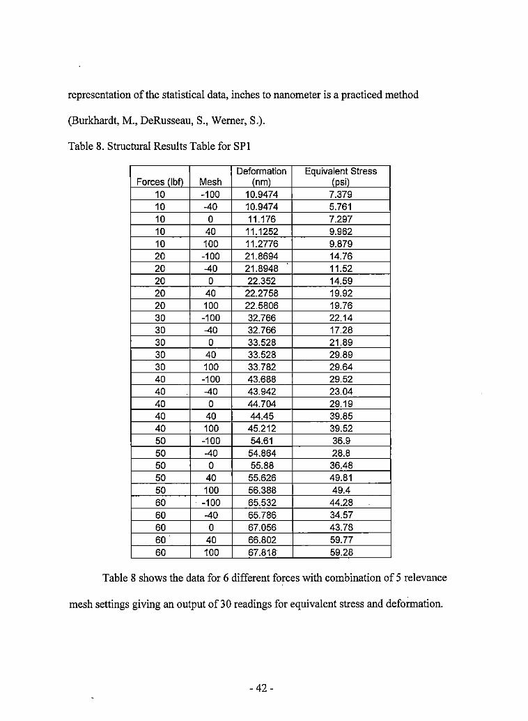
representation of the statistical data, inches to nanometer is a practiced method
(Burkhardt, M., DeRusseau, S., Werner, S.).
Table 8. Structural Results Table for SP!
Deformation Equivalent Stress Forces /lbfl Mesh (nm) lnsi)
10 -100 10.9474 7.379 10 -40 10.9474 5.761 10 0 11.176 7.297 10 40 11.1252 9.962 10 100 11.2776 9.879 20 -100 21.8694 14.76 20 -40 21.8948 11.52 20 0 22.352 14.59 20 40 22.2758 19.92 20 100 22.5806 19.76 30 -100 32.766 22.14 30 -40 32.766 17.28 30 0 33.528 21.89 30 40 33.528 29.89 30 100 33.782 29.64 40 -100 43.688 29.52 40 -40 43.942 23.04 40 0 44.704 29.19 40 40 44.45 39.85 40 100 45.212 39.52 50 -100 54.61 36.9 50 -40 54.864 28.8 50 0 55.88 36.48 50 40 55.626 49.81 50 100 56.388 49.4 60 · -100 65.532 44.28 60 -40 65.786. 34.57 60 0 67.056 43.78 60. 40 66.802 59.77 60 100 67.818 59.28
Table 8 shows the data for 6 different forces with combination of 5 relevance
mesh settings giving an output of 3 0 readings for equivalent stress and deformation.
- 42 -
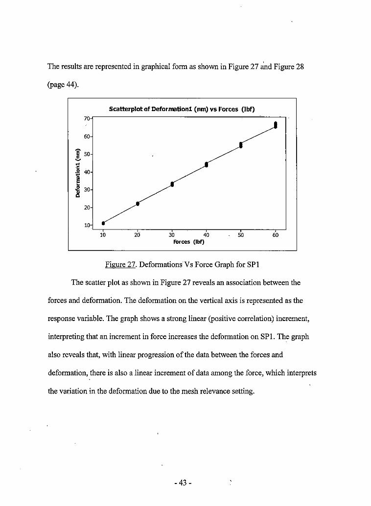
The results are represented in graphical form as shown in Figure 27 ~d Figure 28
(page 44).
Scatterplot of Deformationl (nm) vs Forces (lbf)
10 20 30 40 50 60 Forces (lbf)
Figure 27. Deformations·vs Force Graph for SPl
The scatter plot as shown in Figure 27 reveals an association between the
forces and deformation. The deformation on the vertical axis is represented as the
response variable. The graph shows a strong linear (positive correlation) increment,
interpreting that an increment in force increases the deformation on SP 1. The graph
also reveals that, with linear progression of the data between the forces and
deformation, there is also a linear increment of data among the force, which interprets
the variation in the deformation due to the mesh relevance setting.
-43 -
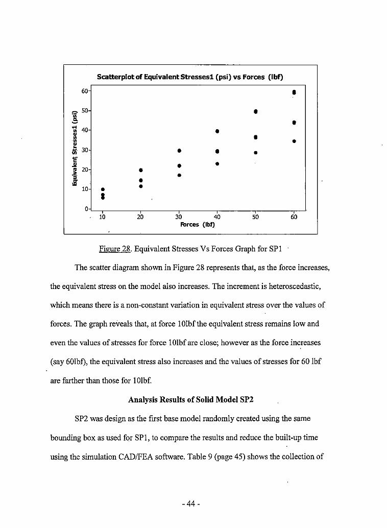
Scatterplot of Equivalent Stressesl (psi) vs Forces (lbf)
60 • 00 50- • "' Cl. • ~ .... 40 ., • .. • ., ., • .. ~
30 ... • • • U) .... C • .!! • .. 20· • .2: • :, ,if •
10- • • I
0-10 20 30 40 50 60
forces (lbf)
Figure 28. Equivalent Stresses Vs Forces Graph for SPl
The scatter diagram shown in Figure 28 represents that, as the force increases,
the equivalent stress on the model also increases. The increment is heteroscedastic,
which means there is a non-constant variation in equivalent stress over the values of
forces. The graph reveals that, at force 1 Olbf the equivalent stress remains low and
even the values of stresses for force 1 Olbf are close; however as the force increases
(say 60lbf), the equivalent stress also increases and the values of stresses for 60 !bf
are farther than those for 1 Olbf.
Analysis Results of Solid Model SP2
SP2 was design as the first base model randomly created using the same
bounding box as used for SPl, to compare the results and reduce the built-up time
using the simulation CAD/FEA software. Table 9 (page 45) shows the collection of
-44 -

results recorded from separate individual simulation of six different forces on SP 1.
Each force was simulated for five different meshes giving the results in the form of
deformations in inches and equivalent stress in psi. The deformation was converted to
nanometer using the conversion of 1 inches = 25400000 nm.
Table 9. Structural Results Table for SP2
Forces Deformation Equivalent Stress (lbf) Mesh (nm) losi)
10 -100 7.9248 1.811 10 -40 8.0772 2.227 10 0 8.255 2.584 10 40 8.3058 3.142 10 100 8.4074 3.325 20 -100 15.8496 3.621 20 -40 16.1544 4.453 20 0 16.51 5.168 20 40 16.637 6.823 20 100 16.7894 6.65 30 -100 23.7998 5.432 30 -40 24.2316 6.68 30 0 24.765 7.753 30 40 24.9428 10.24 30 100 24.9428 10.24 40 -100 31.75 7.242 40 -40 32.258 8.906 40 0 33.02 10.34 40 40 33.274 13.65 40 100 33.528 13.3 50 -100 39.624 9.053 50 -40 40.386 11.13 50 0 41.402 12.92 50 40 41.656 17.06 50 100 41.91 16.62 60 -100 47.498 10.86 60 -40 48.514 13.36 60 0 49.53 15.51 60 40 49.784 20.47 60 100 50.292 19.95
-45 -

Table 9 (page 45) shows the analysis results for SP2 in the form of maximum
equivalent stresses and deformations with respect to forces applied. The results are
shown in the form of graphical representation, using Minitab. Figure 29 represents a
linear progression graph of deformation versus forces showing linear increment in
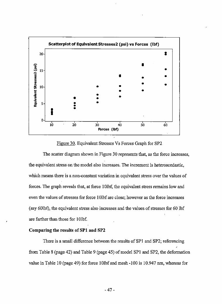
deformation with the increase in force. Figure 30 (page 47) represents the graphical
representation of equivalent stresses versus forces with the linear increment in
stresses with forces.
'e' C ~
"' C
so
40
.S! 30
i i C 20
10
10
Scatterplot of Deformation2 {nm) vs Forces {lbf)
20 30 40 so 60 forces (lbf)
Figure 29 . .Deformations Vs Forces Graph for SP2
The scatter plot shown in Figure 29 shows the linear progression of data,
which -reveals that, as force increases, there is an increment in deformation, showing a
non-constant variation in deformation over the values of forces.
- 46-
Scatterplot of Equivalent Stresses2 (psi) vs Forces (lbf)
20 I
r- I .. C.
15 • ~
N .. • • .. • .. .. ! • • Ii! 10- • • .. • • C J! • .. • • • . 2' :,
5- • • {jf • I •
0 . ' ' 10 20 30 40 50 60 Forces (lbf)
Figure 30. Equivalent Stresses Vs Forces Graph for SP2
The scatter diagram shown in Figure 30 represents that, as the force increases,
the equivalent stress on the model also increases. The increment is heteroscedastic,
which means there is a non-constant variation in equivalent stress over the values of
forces. The graph reveals that, at force 1 Olbf, the equivalent stress remains low and
even the values of stresses for force 1 Olbf are close; however as the force increases
(say 60lbf), the equivalent stress also increases and the values of stresses for 60 lbf
are farther than those for 1 Olbf.
Comparing the results of SPl and SP2
There is a small difference between the results of SPl and SP2; referencing
from Table 8 (page 42) and Table 9 (page 45) of model SPl and SP2, the deformation
value in Table IO (page 49) for force !Olbf and mesh -100 is 10.947 nm, whereas for
- 47 -

the samfe force of 1 Olbf and mesh of -100, the deformation value of SP2 is 7 .925 nm.
The difference is 3.022 nm, which is due to an increase in mass at the applied force
region of SP2. The design with less deformation will be able to hold repeated force
cycles. SP2 is also capable of holding 60lbfwith the deformation of50.292 nm,
whereas SP! shows almost 68 nm. The model SP2 also shows lesser stress than SP!.
Consequently, the model SP2 shows higher stiffness as compared to SP!, but SP2
uses slightly more material than SP!, increasing the volume of the model.
Analysis Results of Solid Model SP3
The structural results in Table IO (page 49) show the data for 6 different
forces with the combination of 5 relevance mesh settings giving output of 3 0 readings
for equivalent stress and deformation. The results are represented in graphical form as
shown in Figure 31 (page 50) and Figure 32 (page 51).
- 48 -

Table 10. Structural Results Table for SP3
Forces Deformation Equivalent Stress llbfl Mesh lnm\ lnsi)
10 -100 8.382 1.866 10 -40 8.5344 2.469 10 0 8.7122 2.34 10 40 8.7884 2.701 10 100 8.8392 3.022 20 -100 16.7386 3.732 20 -40 17.0688 4.937 20 0 17.4244 4.68 20 . 40 17.5514 5.403 20 100 17.6784 6.044 30 -100 25.0952 5.599 30 -40 25.654 7.406 30 0 26.162 7.02 30 40 26.416 8.104 30 100 26.416 9.066 40 -100 33.528 7.465 40 -40 34.036 9.875 40 0 34.798 9.359 40 40 35.052 10.81 40 100 35.306 12.09 50 -100 41.91 9.331 50 -40 42.672 12.34 50 0 43.688 11.7 50 40 43.942 13.51 50 J 100 44..196 15.11 60 -100 50.292 11.2 60 -40 51.308 14.81 60 0 52.324 14.04 60 40 52.578 16.21 60 100 53.086 18.13
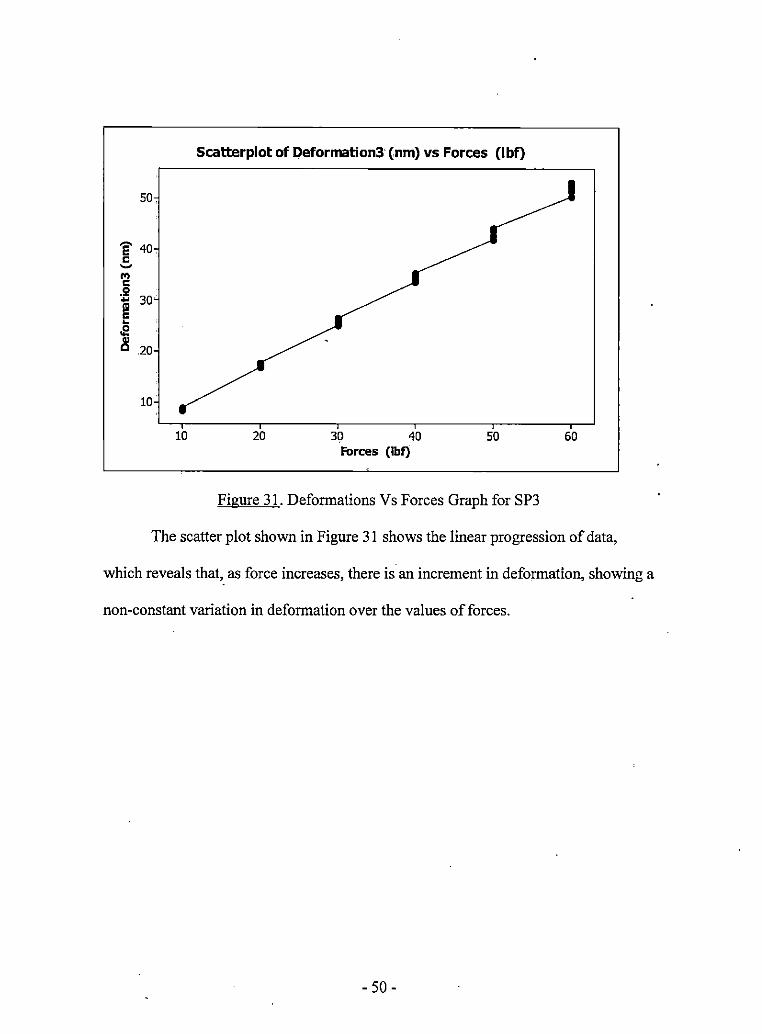
Figure 31 (page 50) shows the scatterplot of deformation versus forces,
interpreting that, as force increases on the SP3, there is a significant increase in
deformation. Figure 32 (page 51) shows'the scatterplot of equivalent stresses versus
forces on SP3.
-49-
Scatterplot of Deformation3· (nm) vs Forces (lbf)
50,
'e' 40, C -i i 30 ~
,E
.!: 20
10
10 20 30 40 50 60 Forces (lbf)
Figure 31. Deformations Vs Forces Graph for SP3
The scatter plot shown in Figure 31 shows the linear progression of data,
which reveals that, as force increases, there is an increment in deformation, showing a
non-constant variation in deformation over the values of forces.
- 50 -
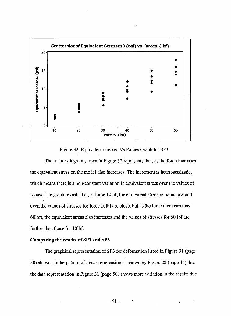
Scatterplot of Equivalent Stresses3 (psi) vs Forces (lbf) 20
• ,::. • a 15- • • ~ • "' • ., GI • • ., • ., • GI • .. 10- I GS • • ... • C .5! I • ,. . 2: • • :, 5- I iii" • I
0-10 20 30 40 50 60
Forces (lbf)
Figure 32. Equivalent stresses Vs Forces Graph for SP3
The scatter diagram shown in Figure 32 represents that, as the force increases,
the equivalent stress on the model also increases. The increment is heteroscedastic,
which means there is a non-constant variation in equivalent stress over the values of
forces. The graph reveals that, at force 1 0lbf, the equivalent stress remains low and
even the values of stresses for force 1 0lbf are close, but as the force increases (say
60Jbf), the equivalent stress also increases and the values of stresses for 60 !bf are
farther than those for 1 Olbf.
Comparing the results of SPl and SP3
The graphical representation of SP3 for deformation listed in Figure 31 (page
50) shows similar pattern ciflinear progression as shown by Figure 28 (page 44), but
the data representation in Figure 31 (page 50) shows more variation in the results due
- 51 -

to mesh, as compared to Figure 28 (page 44). Figure 19 (page 34) shows the same
consistent non-constant variation, whereas Figure 29 (page 46) shows more variation
in the values of mesh 0 and 40. The deformation value in Table 7 for force 1 0lbf and
mesh-100 is 10.947 nm, whereas for the same force of lOlbf and mesh of-100, the
deformation value of SP3 is 8.382 nm. The equivalent stress values of SP3 are less
than that of the equivalent stress of SP 1. Hence, considering the result parameters,
model SPl has a greater (or a lesser) maximum percent rate of failure due to repeated
force than model SP3.
Analysis Results of Solid Model SP4
Table 11 (page 53) shows the data for 6 different forces with a combination of
5 relevance mesh settings, giving an output of 30 readings for equivalent stress and
deformation.
- 52 -
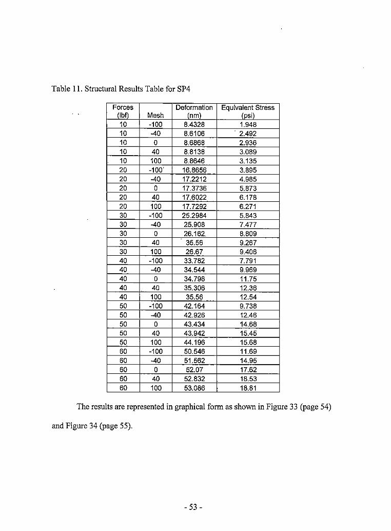
Table 11. Structural Results Table for SP4
Forces Deformation Equivalent Stress (lbf) Mesh (nm) (osi} 10 -100 8.4328 1.948 10 -40 8.6106 . 2.492 10 0 8.6868 2.936 10 40 8.8138 3.089 10 100 8.8646 3.135 20 -100' 16.8656 3.895 20 -40 17.2212 4.985 20 0 17.3736 5.873 20 40 17.6022 6.178 20 100 17.7292 6.271 30 -100 25.2984 5.843 30 -40 25.908 7.477 30 0 26.162. 8.809 30 40 35.56 9.267 30 100 26.67 9.406 40 -100 33.782 7.791 40 -40 34.544 9.969 40 0 34.798 11.75 40 40 35.306 12.36 40 100 35.56 12.54 50 -100 42.164 9.738 50 -40 42.926 12.46 50 0 43.434 14.68 50 40 43.942 15.45 50 100 44.196 15.68 60 -100 50.546 11.69 60 -40 51.562 14.95 60 0 52.07 17.62 60 40 52.832 18.53 60 100 53.086 18.81
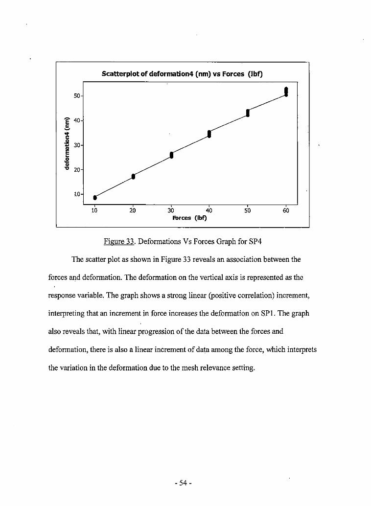
The results are represented in graphical form as shown in Figure 33 (page 54)
and Figure 34 (page 55).
- 53 -
so
'e 40 C ~
1: :8 30 ~ ~ .e
_g 20
10
10
Scatterplot of deformation4 (nm) vs Forces (lbf)
20 30 40 50 60 forces (lbf)
Figure 33. Deformations Vs Forces Graph for SP4
The scatter plot as shown in Figure 33 reveals an association between the
forces and deformation. The deformation on the vertical axis is represented as the
response variable. The graph shows a strong linear (positive correlation) increment,
interpreting that an increment in force increases the deformation on SP 1. The graph
also reveals that, with linear progression of the data between the forces and
deformation, there is also a linear increment of data among the force, which interprets
the variation in the deformation due to the mesh relevance setting.
- 54 -

Scatterplot of Equivalent Stresses4 (psi) vs Forces (lbf)
20-
I •
,=. • Ill 15- • ... • ---,t Ill
I • ., Ill • Ill
~ 10 • til I • ... C • • .!l! .. I .a: • :, 5- • ,B' • I
0 10 20 30 40 50 60
Forces (lbf)
Figure 34. Equivalent Stresses Vs Forces Graph for SP4
The scatter diagram shown in Figure 34 represents that, as the force increases,
the equivalent stress on the model also increases. The increment is heteroscedastic,
which means there is a non-constant variation in equivalent stress over the values of
forces. The graph reveals that, at force 1 Olbf, the equivalent stress remains low and
even the values of stresses for force 1 Olbf are close, but as the force increases (say
60lbf), the equivalent stress also increases and the values of stresses for 60 !bf are
farther than those for 1 Olbf.
- 55 -

Comparing the results of SPl and SP4
According to the results, model SP4 shows maximum stiffness as compared to
model SP!, as the deformation of SP4 at force !0lbfand mesh-100 is 8.433 nm,
compare to the deformation ofSPI, which is 10.947 nm. Also model SP! shows
maximum equivalent stress as compared to the equivalent stress of SP4. Hence, from
the results, SP4 has maximum resistance against the repeated force as compared to
SP!.
Analysis Results of Solid Model SPS
Table 12 (page 57), shows the data for 6 different forces with a combination of
5 relevance mesh settings giving output of 30 readings for equivalent stress and
deformation.
- 56 -

Table 12. Structural Results Table for SP5
Forces Deformation Equivalent (lbfl Mesh (nm) Stress r nsi) 10 -100 14.3002 3.676 10 -40 14.5288 4.141 10 0 14.5796 4.548 10 40 14.6558 4.955 10 100 14.7574 5.218 20 -100 28.702 7.352 0 -40 28.956 8.282
20 0 29.21 9.096 20 40 29.21 9.909 20 100 29.464 10.44 30 -100 42.926 11.03 30 -40 43.688 12.42 30 0 43.688 13.64 30 40 43.942 14.86 30 100 44.196 15.65 40 -100 57.15 14.7 40 -40 58.166 16.56 40 0 58.42 18.19 40 40 58.674 19.82 40 100 58.928 20.87 50 -100 71.628 18.38 50 -40 72.644 20.7 50 0 72.898 22.74 50 40 73.152 24.77 50 100 73.66 26.09 60 -100 85.852 22.06 60 -40 87.122 24.85 60 0 87.376 27.29 60 · 40 87.884 29.73 60 100 88.646 31.31
The results are represented in graphical form as shown in Figure 35 (page 58)
and Figure 36 (page 59).
- 57 -

Scatterplot of deformations (nm) vs Forces (lbf)
90
80
'E' 70
C ..... 60 "' C
:8 50 ~ ..
40 .E CIJ
"CJ 30
20
10
10 20 30 40 50 60 Forces (lbf)
Figure 35. Deformations Vs Forces Graph for SP5
The scatter plot shown in Figure 35 shows the linear progression of data,
which reveals that, as force increases, there is an increment in deformation, showing a
non-constant variation in deformation over the values of forces.
- 58 -

Scatterplot of Equivalent StressesS (psi) vs Forces (lbf) 35-
30- • • r=- • ig_ 25- • - • • In • .. • GJ .. 20- : • ..
GJ • • ~
il'i I • .. 15- • C • .gj • "' • .2: 10- I :, ,8"
5- I 0-
' ' 30 4'0 10 20 50 60 Forces (lbf)
Figure 36. Equivalent Stresses Vs Forces Graph for SP5
The scatter diagram shown in Figure 36 represents that, as the force increases,
the equivalent stress on the model also increases. The increment is heteroscedastic,
which means there is a non-constant variation in equivalent stress over the values of
forces. The graph reveals that, at force 1 Olbf, the equivalent stress remains low and
even the values of stresses for force I Olbfare close, but as the force increases (say
60lbf), the equivalent stress also increases and the values of stresses for 60 !bf are
farther than those for I 01 bf.
- 59 -
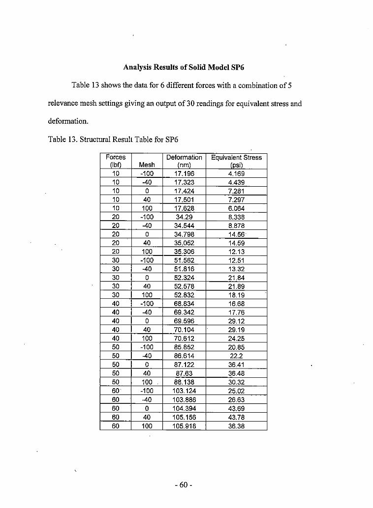
Analysis Results of Solid Model SP6
Table 13 shows the data for 6 different forces with a combination of 5
relevance mesh settings giving an output of 30 readings for equivalent stress and
deformation.
Table 13. Structural Result Table for SP6
Forces Deformation Equivalent Stress rJbfl Mesh lnml lnsil 10 -100 17.196 4.169 10 -40 17.323 4.439 10 0 17.424 7.281 10 40 17.501 7.297 10 100 17.628 6.064 20 -100 34.29 8.338 20 -40 34.544 8.878 20 0 34.798 14.56 20 40 35.052 14.59 20 100 35.306 12.13 30 -100 51.562 12.51 30 -40 51.816 13.32 30 0 52.324 21.84 30 40 52.578 21.89 30 100 52.832 18.19 40 -100 68.834 16.68 40 -40 69.342 17.76 40 0 69.596 29.12 40 40 70.104 29.19 40 100 70.612 24.25 50 -100 85.852 20.85 50 -40 86.614 22.2 50 0 87.122 36.41 50 40 87.63 36.48 50 100 88.138 30.32 60 -100 103.124 25.02 60 -40 103.886 26.63 60 0 104.394 43.69 60 40 105.156 43.78 60 100 105.918 36.38
- 60 -

The results are represented in graphical form as shown in Figure 3 7 and Figure 3 8
(page 62).
Scatterplot of deformation6 (nm) vs Forces (lbf) 110
100
90
'e' 80 C -"' 70 C
.Sl 60 ..
~ .. 50 ,E QI
'ti 40
30
20
10 20 30 40 50 60 Forces (lbf)
Figure 37. Deformations Vs Forces Graph for SP6
The scatter plot a~ shown in Figure 3 7 reveals an association between the
forces and deformation. The deformation on the vertical axis is represented as the
response variable. The graph shows a strong linear (positive correlation) increment,
interpreting that an increment in force increases the deformation on SP I. The graph
also reveals that, with linear progression of the data between the forces and
deformation, there is also a linear increment of data among the forces, which
interprets the variation in the deformation due to the mesh relevance setting.
- 61 -
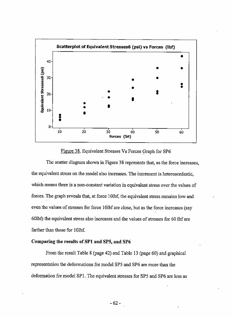
40
"" <II Q, ~
ID 30· <II .. <II <II .. ... lil 20 .. C
.l!! ..
.2! :,
iB" 10·
0
Scatterplot of Equivalent Stresses& (psi) vs Forces (lbf)
•
• • • • :
• I • • •
: • • ' ' ' 10 20 30 40 50
Forces (lbf)
Figure 38. Equivalent Stresses Vs Forces Graph for SP6
• •
• •
' 60
The scatter diagram shown in Figure 3 8 represents that, as the force increases,
the equivalent stress on the model also increases. The increment is heteroscedastic,
which means there is a non-constant variation in equivalent stress over the values of
forces. The graph reveals that, at force I 0lbf, the equivalent stress remains low and
even the values of stresses for force I Olbf are close, but as the force increases (say
60lbf) the equivalent stress also increases and the values of stresses for 60 !bf are
farther than those for I Olbf.
Comparing the results of SPI and SPS, and SP6
From the result Table 8 (page 42) and Table 13 (page 60) and graphical
representation the deformations for model SP5 and SP6 are more than the
deformation for model SP!. The equivalent stresses for SP5 and SP6 are less as
- 62 -

compared to the equivalent stress of SP 1. The comparison of the design model is
based on the results obtained from processing of each individual design. These data
are collected and organized in tabular form to understand the relationship between the
results and identify the optimized or optimal design based on the simulation
technique, considering deformation and equivalent stresses.
Mathematical Design:
The design used was a 3 factor factorial model for deformation and equivalent
stresses. The following model was used to relate the response variable with the other
factors.
Response= µ+D+F+M+D * F+D * M+F * M+E
Where,
D represents Design effects.
F represents Force effects.
M represents Mesh effects.
E represents Error.
µ represents an overall average response deformation ( equivalent stresses)
D*F represents an interaction effect between design and force.
D*M represents an interaction effect between design and mesh.
F*M represents an interaction effect between force and mesh.
Note: The D*F*M.term was omitted from the model. This was added to the error
term.
- 63 -

Analysis of Variance Output for the Model When Deformation is the Response
Variable.
Factor Type Levels Values Design fixed 6 D1, D2, D3, D4, D5, D6 Forces (lbf) fixed 6 10, 20, 30, 40, SO, 60 Mesh fixed 5 -100, -40, o, 40, 100
Analysis of Variance for Deformations (run), using Adjusted SS for Tests
Source DF Seq SS Adj ss Adj MS F p Design 5 26283.3 26283.3 5256. 7 669702.97 0.000 Forces (lbf) 5 68617.0 68617.0 13723. 4 1748375.93 0.000 Mesh 4 50.7 50.7 12.7 1615.19 0.000 Design*Forces (lbf) 25 6268.4 6268. 4 250.7 31943.93 0.000 Design*Mesh 20 2.0 2.0 0.1 12.77 0.000 Forces (lbf) *Mesh 20 12.4 12.4 0.6 78.76 0.000 Error 100 0.8 0.8 0.0 Total 179 101234.6
S = 0.0885959 R-Sq = 100.00% R-Sq(adj) 100.00%
Unusual Observations for Deformations (run)
Obs Deformations (run) Fit SE Fit Residual St Resid 1 10.947 11.092 0.059 -0.145 -2.19 R 4 11.125 10.968 0.059 0.157 2.38 R
14 33.528 33.393 0.059 0.135 2.05 R 26 65.532 65.385 0.059 0.147 2.23 R 29 66.802 66.958 o. 059 -0.156 -2.36 R
119 52.832 52. 688 0.059 0.144 2.18 R 122 14.529 14.684 0.059 -0.155 -2.35 R 127 28.956 29 .108 0.059 -0.152 -2.30 R 178 104.394 104.548 0.059 -0.154 -2.33 R
R denotes an observation with a large standardized residual.
Figure 39. Analysis of Variance Output for the Model When Deformation is the
Response Variable.
Figure 39 first displays factors (design, forces, and mesh), their types (all
fixed), number oflevels, and the level values. The second table gives an analysis of
variance table. This is followed by a table of coefficients, and then a table of unusual
observations.
- 64-

s 20.75 R-Sq 25.96% R-Sq(adj) - 23.84%
Level N Mean StDev D1 30 38.84 19.29 D2 30 28. 67 14.24 D3 30 30.27 15.05 D4 30 30.38 15.07 D5 30 50.97 25.30 D6 30 60.95 30.27
Pooled StDev 20.75
Individual 95% Cis For Mean Based on Pooled StDev --+---------+---------+---------+-------
(-----*------) (-----*-----) (-----*-----) (-----*------)
(-----*------)
(-----*-----) --+---------+---------+---------+-------
24 36 48 60
Tukey 95% Simultaneous Confidence Intervals All Pairwise Comparisons among Levels of Design
Individual confidence level= 99.56%
Design= D1 subtracted from:
Design D2 D3 D4 D5 D6
Design
Design D3 D4 D5 D6
Design
Design D4 D5 D6
Lower Center Upper -25.63 -10.17 5.29 -24.03 -8.57 6. 89 -23.92 -8.46 7.00 -3.33 12.13 27.59
6.65 22.11 37.57
D2 subtracted from:
Lower Center Upper -13.85 1. 61 17.07 -13.75 1. 71 17.17
6.84 22.30 37.76 16.82 32.28 47.74
D3 subtracted from:
Lower -15.35
5.23 15.22
Center 0.11
20.69 30.68
Upper 15.57 36.15 46 .14
---------+---------+---------+---------+ (-----*-----) (------*-----) (------*-----)
(-----*-----) (-----*-----)
---------+---------+---------+---------+ -25 0 25 50
---------+---------+---------+---------+ (------*-----) (-----*-----)
(-----*-----) (-----*-----)
---------+---------+---------+---------+ -25 0 25 50
---------+---------+---------+---------+ (-----*-----)
(-----*-----) (-----*-----)
------+---------+---------+---------+ -25 0 25 50
- 66 -

Design= D4 subtracted from:
Design D5
Lower Center Upper 5.13 20.59 36.05
15.11 30.57 46.03
---------+---------+---------+---------+· (-----•-----)
(-----*-----) D6
---------+---------+---------+---------+ -25 0 25 50
Design= DS subtracted from:
Design Lower Center Upper ---------+---------+---------+---------+ D6 -5.48 9.98 25.44 (-----*-----)
---------+---------+---------+---------+ -25 0 25 50
Figure 40. Tukey's Multiple Comparison for Average Deformation for the Six Different Models
Figure 40 shows the P-value is 0.000 for design, indicating that there is
sufficient evidence of equality between the means when the level of significance is
set at 0.05, which confirms to reject the hypothesis of no difference. The difference
between the means is shown in Tukey 95% simultaneous confidence intervals for all
Pairwise Comparisons among the six designs.
Tukey's Comparisons
Tukey' s test provides 5 sets of multiple comparison confidence intervals.
• Design I mean substracted from design 2, 3, 4, 5, and 6 means: The first
interval in the first set of the Tukey's output (-25.63, 5.29) gives the
confidence interval for the average of design! subtracted from the average of
design 2. For this set of comparisons, none of the means is statistically
different because all of the confidence intervals include 0. The means for
- 67 -
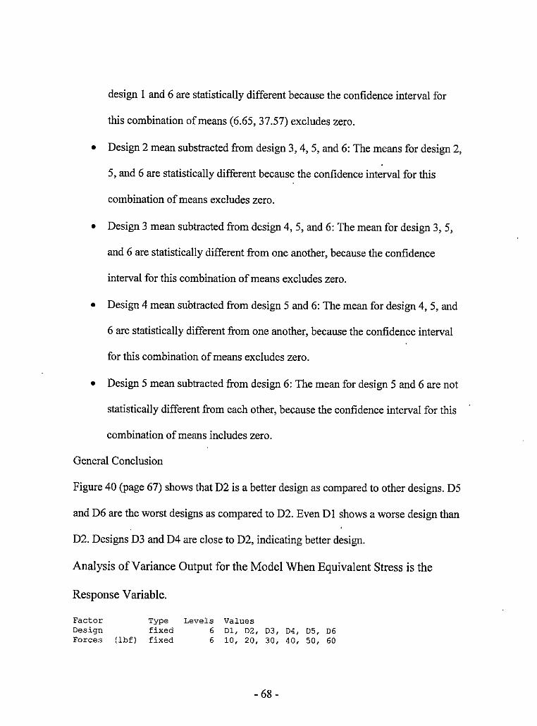
design I and 6 are statistically different because the confidence interval for
this combination of means (6.65, 37.57) excludes zero.
• Design 2 mean substracted from design 3, 4, 5, and 6: The means for design 2,
5, and 6 are statistically different because the confidence interval for this
combination of means excludes zero.
• Design 3 mean subtracted from design 4, 5, and 6: The mean for design 3, 5,
and 6 are statistically different from one another, because the confidence
interval for this combination of means excludes zero.
• Design 4 mean subtracted from design 5 and 6: The mean for design 4, 5, and
6 are statistically different from one another, because the confidence interval
for this combination of means excludes zero.
• Design 5 mean subtracted from design 6: The mean for design 5 and 6 are not
statistically different from each other, because the confidence interval for this
combination of means includes zero.
General Conclusion
Figure 40 (page 67) shows that D2 is a better design as compared to other designs. D5
and D6 are the worst designs as compared to D2. Even DI shows a worse design than
D2. Designs D3 and D4 are close to D2, indicating better design.
Analysis of Variance Output for the Model When Equivalent Stress is the
Response Variable.
Factor Design Forces (lbf)
Type fixed fixed
Levels Values 6 D1, D2, D3, D4, D5, D6 6 10, 20, 30, 40, so, 60
- 68 -

Mesh fixed 5 -100, -40, 0, 40, 100
Analysis of Variance for Equivalent Stresses (psi), using Adjusted SS for Tests
Source OF Seq SS Adj ss Adj MS F p Design 5 9177. 70 9177.70 1835.54 942.80 0.000 Forces (lbf) 5 10080. 72 10080.72 2016.14 1035.57 0.000 Mesh 4 1200.06 1200.06 300.02 154.10 0.000 Design*Forces (lbf) 25 2183.61 2183.61 87,34 44.86 0.000 Design*Mesh 20 818.00 818.00 40.90 21. 01 0.000 Forces (lbf) *Mesh 20 286.73 286.73 14.34 7.36 0.000 Err6r 100 194.69 194.69 1. 95 Total 179 23941.50
S ~ 1.39531 R-Sq ~ 99.19% R-Sq(adj) 98.54%
Unusual Observations for Equivalent Stresses (psi}
Equivalent Stresses
Obs (psi) Fit SE Fit Residual St Resid 2 5.7610 2.0137 0.9302 3 .. 7 4 7 3 3.60 R 3 7.2970 5 .1148 0.9302 2.1822 2 .10 R· 4 9. 9620 12.5607 0.9302 -2.5987 -2.50 R 5 9.8790 12.6256 0.9302 -2.7466 -2.64 R 7 11.5200 9.2662 0.9302 2.2538 2.17 R
22 28.8000 .31.0543 0.9302 -2.2543 -2.17 R 27 34.5700 38.3207 0.9302 -3.7507 -3.61 R 28 43.7800 45.9723 0.9302 -2.1923 -2 .11 R 29 59. 7700 57.1516 0.9302 2. 6184 2.52 R 30 59.2800 56. 5286 0.9302 2.7514 2. 65 R
153 7.2810 10.5749 0.9302 -3.2939 -3.17 R 178 43.6900 40.4020 0.9302 3.2880 3.16 R
R denotes an observation with a large standardized residual.
Figure 41. Analysis of Variance Output for the Model When Equivalent Stress is the
Response Variable.
In Figure 41, all p-values are printed as 0.000, meaning that they are less than
0.0005. This indicates significant evidence of effects if the level of significance, a, is
greater than 0.0005. The significant interaction effects of deformation with design,
forces, and mesh terms imply that the coefficients of second order regression models
of the effect of forces and mesh upon deformation depend upon the design. The R-
- 69-

square value shows that the model explains 99 .19% of the variance in equivalent
stresses, indicating that the model fits the data extremely well for predicting
deformation from design, forces, and mesh factors.
Tukey's Multiple Comparison for Average Equivalent Stress for Six Different
Models.
Source Design Error Total
DF SS 5 9177. 7
174 14763.8 179 23941.5
MS 1835.5
84.8
F 21. 63
p
0.000
S ~ 9.211 R-Sq ~ 38_. 33% R-Sq(adj) 36.56%
Individual 95% Cis For Mean Based on Pooled StDev
Level Dl
N 30 30 30 30 30 30
Mean StDev --+---------+---------+---------+-------
D2 D3 D4 D5 D6
28.195 9.351 8. 679 9.521
15. 77 6 20.475
15.409 5.262 4.569 5.047 8.131
11. 468
Pooled StDev = 9.211
(---*----) (---*----)
(---*----) (----*---)
(----*---)
(---*----)
--+---------+---------+---------+-------7.0 14.0 21.0 28.0
Tukey 95% Simultaneous Confidence Intervals All Pairwise•Cornparisons among Levels of Design
Individual confidence level= 99.56%
Design D1 subtracted from:
Design D2 D3 D4 D5 D6
Lower -25.706 -26.378 -25.536 -19.281 -14.582
Center ·-18.845 -19.516 -18.675 -12.419 -7. 720
Upper -11. 983 -12. 655 -11. 813 -5.558
--+---------+---------+---------+-------(----*-----)
(-----*----) (----*-----)
(-----*----) -0.858 ' (-----*----)
--+---------+---------+---------+--------24 -12 ·o 12
Design 02 subtracted from:
Design Lower D3 -7.533 D4 -6.692 D5 -0.436
Center -0.672
0.170 6.425
Upper 6.190 7. 032
13.287
--+---------+---------+---------+-------
- 70-
(----*-----) (-----*-----)
(----*-----)

D6 4.263 11.125 17.986
Design= D3 subtracted from:
Design Lower Center D4 -6.020 0.842 D5 0.235 7.097 D6 4.935 11.796
Upper 7.703
13.959 18.658
Design= D4 subtracted from:
Design D5 D6
Lower -0.606
4. 093
Center 6.255
10.954
Upper 13.117 17. 816
Design= D5 subtracted from:
(----*-----)
--+---------+---------+---------+--------24 -12 0 . 12
--+---------+---------+----.----+-------(-----*----)
(-----*-----) (-----*-----)
--+---------+---------+---------+--------24 -12 0 12
--+---------+---------+---------+-------(-----*-----)
(-----*-----)
--+---------+---------+---------+--------24 -12 0 12
Design Lower Center Upper --+---------+---------+------- --+-------D6 -2.162 4.699 11.561 (-----*-----)
--+---------+---------+---------+--------24 -12 0 12
Figure 42. Tukey's Multiple Comparison for Average Equivalent Stress for Six
Different Models Result Interpretation
Figure 42 shows the P-value is 0.000 for design and indicates that there is
sufficient evidence of no equality between the means when alpha is set at 0.05, which
confirms to reject the hypothesis of no difference. The difference between the means
is shown in Tukey 95% simultaneous confidence intervals all Pairwise Comparisons
among Levels of Design.
Tukey's Comparisons
Tukey' s test provides 5 sets of multiple comparison confidence intervals.
- 71 -

• Design 1 mean substracted from design 2, 3, 4, 5, and 6 means,: For this set of
comparisons, none of the means is statistically different because all of the
confidence intervals include 0.
• Design 2 mean substracted from design 3, 4, 5, and 6: The means for design 2
and 6 are statistically different because the confidence interval for this
combination of means excludes zero.
• Design 3 mean substracted from design 4, 5, and 6: The mean for design 3, 5,
and 6 are statistically different from one another, because the confidence
interval for this combination of means excludes zero.
• Design 4 mean substracted from design 5 and 6: The mean for design 4 and 6
are statistically different from one another, because the confidence interval for
this combination of means excludes zero.
• Design 5 mean substracted from design 6: The mean for design 5 and 6 are
not statistically different from each other, because the confidence interval for
this combination of means includes zero (Joiner, R).
General Conclusion
Figure 42 (page 71) shows that D3 is the most efficient design as compared to other
designs. Figure 42 (page 71) also shows that DI is the worst design, when compared
with D3. D5 and D6 also show worse design.
- 72-

Conclusion
It has been shown by the simulation using CAD modeling and finite element
analysis integration and confirmed by the results, a time consuming design formation
and optimization of the designed model were possible. The prediction of deformation
and stress was the major factor in designing an optimized model. Without using.
CAD/PEA for design modification and one-click transformation to stress analysis
environment to predict the deformation and stress, the designers will have to sacrifice
their time and money in testing physical models. To be able to obtain the final design
and meet the strength requirements, 6 design models were created and analyzed for 6
different forces and 5 different mesh settings obtaining 30 results for deformation and
equivalent stresses each. Without CAD/PEA it would have taken months to design
these models, build each for the physical model, and test for the analysis.
The analysis results shown by the result table and the general conclusion from
the analysis of variance of deformation and equivalent stresses entails that model SP3
shows relatively optimized design as compared to the results of other design models.
The results also show that the model does not necessarily have to be heavy to sustain
force, but design plays an important role in sustaining force to reduce deformation.
Therefore, an optimal design should incorporate a combination of good control over
the geometry.
- 73 -

Suggestions and Recommendations
There are several other methods to optimize the design.
1. The next step for the further research is considering the material selection
factor. Material selection also affects the cost and appearance of the product.
Best material selection could result in reduced deformation and stresses for
the same forces.
2. Vibration effect consideration is another factor to be researched to
manufacture a product.
3. Temperature affects when the vise is holding a part under the CNC machine
for longer machining operations.
Limitations
The prediction in this kind of CAD/FEA integration is limited to uniformly
distributed load only. Also the nodes and element settings are selected automatically
for the set relevance mesh setting, which makes it difficult to obtain precise readings
from the congested features.
Future Development on CAD/FE.A Integration
I. The designer should be able to customize the elements and nodes selection to
configure the precise stress and deformation in the part.
2. The CAD/FEA integration should have the ability to choose the nodes and
configure the results on each node selected.
- 74-

Reference
Anderson, D. M. (2004). Design for Manufacturability and Concurrent
Engineering. California: CIM Press.
Bahr, D. F., Moody N. R. ((2005). Development of Experimental Verification
Techniques for Non-linear Deformation and Fracture on the Nanometer Scale.
California: Sandia National Laboratories.
Benhabib, Beno (2003). Manufacturing: Design, Production, Automation, and
Integration. Marcel Dekker Inc.
Black, J. T., DeGarmo, Kohser, E. P ., Ronald A. (1997). Materials and
Processes in Manufacturing. New Jersey: Prentice Hall.
Burkhardt, M. R., DeRusseau, S. N., Werner, S. L. U.S. Geological Survey.
Open-File Report 96-216. (http://ca.water.usgs.gov/pnsp/rep/ofr962l6.pdf).
Groover, P. M., Zimmers, W. E., (1989). Computer Aided Design and
Computer Aided Manufacturing. New Delhi: Prentice Hall oflndia.
Hughes, J. R. (2000). The Finite Element Method Linear Static and Dynamic
Finite Element Analysis. New York: Dover Publications, Inc.
Hryniewiecki, J. (2005). Stress Analysis in Automotive Brake Vacuum
Booster. Indiana: University of Notre Dame.
Joiner, R. (1994). Minitab Handbook, Third Edition. California: International
Thomson Publishing.
- 75 -

Lin, F., Sun, W. (2001). Computer Modeling and FEA Simulation for
Composite Single Fiber Pull-out. Journal of Thermoplastic Composite Materials, Vol.
14 (4), pp.327-343.
Lund, E. (1994). Finite Element Based Design Sensitivity Analysis and
Optimization, Report no. 23. Denmark; Aalborg University.
Madsen, P. D. (2003). Autodesk Inventor 5/5.3 Basics Through Advanced.
New Jersey: Prentice Hall.
Moaveni, S. (1999). Finite Element Analysis Theory and Application with
ANSYS. New Jersey: Prentice Hall.
Rao, S. S. (1999). The Finite Element Method in Engineering. Boston:
Butterworth Heinemann.
Rutherford, A. (2001). Introducing ANOVA and ANCOVA a GLM
Approach. Great Britain: Sage Publications.
- 76-