CACHE's Role in Computing in Chemical Reaction Engineering · University of Washington’s Chemical...
50
103 CACHE’S ROLE IN COMPUTING IN CHEMICAL REACTION ENGINEERING H. Scott Fogler University Of Michigan Ann Arbor, Michigan 48109 Abstract Throughout the last 25 years CACHE has either initiated, nurtured, or financially sup- ported projects to enhance courses in chemical reaction engineering and, as a result, has been instrumental in the evolution of chemical reaction engineering education. Five major CACHE-assisted projects involving computer modules, and/or interactive simu- lations are discussed. Specifically, we focus on early computer programs, the Univer- sity of Michigan Projects, the Purdue University Modules, POLYMATH, and the University of Washington’s Chemical Reactor Design Tool. Introduction CACHE has played many roles in the incorporation of computing in Chemical Reaction Engineering (CRE). It has been an initiator of projects, such as the computer programs in chem- ical reaction engineering (1972), and the set of six CHEMI books on Kinetics (1976-1979), it has been a distributor of programs such as POLYMATH and the Michigan Interactive Kinetics modules. CACHE has also been a mentor and facilitator in the development of these materials, providing both financial, and intellectual resources through collaboration, not only with CACHE trustees, but also with many colleagues in the United States, Canada, and overseas. This paper highlights five areas in which CACHE has played a major role in the advancement of chemical reaction engineering education: the computer programs, the University of Michi- gan’s Interactive Kinetics modules, the Purdue University’s Simulations, the University of Washington’s Chemical Reactor Design Tool, and POLYMATH. Early Computer Programs One of the very first CACHE projects involving the development of computer programs in the areas of chemical reactor design, control design, transport, stoichiometry, and thermody- namics. The programs were written by college faculty and sent on punched cards for evaluation to the appropriate area editor. Professor Matt Reilly was the area editor for kinetics and reactor design, and set the standards for accepting programs by running them in every way possible to try to get them to fail. If a program passed Matt’s rigorous testing, a source program listing and sample output were included in the published volume (Reilly, 1972). A list of the programs and
Transcript of CACHE's Role in Computing in Chemical Reaction Engineering · University of Washington’s Chemical...

103
CACHE’S ROLE IN COMPUTING IN CHEMICAL REACTION ENGINEERING
H. Scott FoglerUniversity Of Michigan
Ann Arbor, Michigan 48109
Abstract
Throughout the last 25 years CACHE has either initiated, nurtured, or financially sup-ported projects to enhance courses in chemical reaction engineering and, as a result, hasbeen instrumental in the evolution of chemical reaction engineering education. Fivemajor CACHE-assisted projects involving computer modules, and/or interactive simu-lations are discussed. Specifically, we focus on early computer programs, the Univer-sity of Michigan Projects, the Purdue University Modules, POLYMATH, and theUniversity of Washington’s Chemical Reactor Design Tool.
Introduction
CACHE has played many roles in the incorporation of computing in Chemical ReactionEngineering (CRE). It has been an initiator of projects, such as the computer programs in chem-ical reaction engineering (1972), and the set of six CHEMI books on Kinetics (1976-1979), ithas been a distributor of programs such as POLYMATH and the Michigan Interactive Kineticsmodules. CACHE has also been a mentor and facilitator in the development of these materials,providing both financial, and intellectual resources through collaboration, not only withCACHE trustees, but also with many colleagues in the United States, Canada, and overseas.This paper highlights five areas in which CACHE has played a major role in the advancementof chemical reaction engineering education: the computer programs, the University of Michi-gan’s Interactive Kinetics modules, the Purdue University’s Simulations, the University ofWashington’s Chemical Reactor Design Tool, and POLYMATH.
Early Computer Programs
One of the very first CACHE projects involving the development of computer programsin the areas of chemical reactor design, control design, transport, stoichiometry, and thermody-namics. The programs were written by college faculty and sent on punched cards for evaluationto the appropriate area editor. Professor Matt Reilly was the area editor for kinetics and reactordesign, and set the standards for accepting programs by running them in every way possible totry to get them to fail. If a program passed Matt’s rigorous testing, a source program listing andsample output were included in the published volume (Reilly, 1972). A list of the programs and

104 COMPUTERS IN CHEMICAL ENGINEERING EDUCATION
authors is shown in Table 1.
Table 1. CACHE Computer Programs for Chemical Engineering Education: Kinetics (1972)
1. BATCH REACTORS
1.1 Complex Reaction System in a Batch Reactor by Jaime P. Ampaya and Robert G. Rinker
1.2 Batch Decomposition of Acetylated Castor Oil by Joseph J. Perona
1.3 Series of Reactions in a Batch Reactor or in a Sequence of Stirred Tank Reactors by R. Rajagopalan
2. CONTINUOUS STIRRED-TANK REACTORS
2.1 Molecular Weight Distribution in a Polymerization Reactor Sequence by James L. Kuester
2.2 Dynamic Mass and Energy Balances in a CSTR by Ephraim Kehat
3. HOMOGENEOUS TUBULAR REACTORS
3.1 Tubular Reactor Design with Two Consecutive Reactions by E. H. Crum
3.2 Chemical Equilibrium and Reaction Rate Conflict by Billy C. Crynes and Barney L. Ghiglieri
3.2 Plug Flow Reactor with Dispersion by George M. Homsy
4. HETEROGENEOUS CATALYSIS
4.1 Effectiveness Factor for a Spherical Catalyst Pellet by Joseph S. Naworski
4.2 Non-Isothermal Catalyst Pellet by Ran Abed and Robert G. Rinker
4.3 Computer-Administered Programmed Instruction in Effectiveness Factors by James T. Cobb, Jr., andThomas Gestrich
5. CATALYTIC REACTORS
5.1 Analysis of Catalytic Reactions in a Packed Bed Reactor by Thomas Z. Fahidy
5.2 Design of a Fixed-Bed Reactor by Charles N. Satterfield and Russell L. Jones
5.3 Design of Non-Isothermal Flow Reactor by William J. Hatcher, Jr.
5.4 Adiabatic Catalytic Reactor Design for Methanol Synthesis: High Pressure by Kermit L. Holman
6. REACTOR DESIGN AND OPTIMIZATION
6.1 Air Sparged Reactor Design by Louis L. Edwards
6.2 SO2 Oxidation Reactor Simulation Program by Donald B. Wilson and Robert L. Hair
6.3 Optimal Selection of a Blend of Two Catalysts in a Tubular Reactor by Michael S. K. Chen
7. EXPERIMENTAL DATA ANALYSIS
7.1 Data Correlation via Non-Linear Regression by George W. Roberts
7.2 Residence-Time Distribution Computation for Flow Processes by William C. Clements, Jr.
The University of Michigan Projects
In 1976, approximately three years after the computer programs listed in Table 1 werepublished and distributed to chemical engineering departments across the nation, a secondproject was completed. With the aide of a grant from the Olin Corporation, five interactive pro-grams, listed below, were developed at the University of Michigan by Professor H. Scott Foglerand a junior in chemical engineering, T. Michael Duncan (now a professor at Cornell).
CACHE’s Role in Computing in Chemical Reaction Engineering 105
1. Rate Laws
2. Stoichiometry
3. Heterogeneous Catalysis
4. Columbo (Murder in a CSTR)
5. Death by Dying (Analysis of Rate Law Data)
These programs were made available for testing by students in the chemical reaction en-gineering course during the 1976-77 academic year. The response and enthusiasm for the mod-ules was overwhelming. These modules were demonstrated at the Summer School forChemical Engineering Faculty held in Snowmass, Colorado during the summer of 1977. Theresponse of the faculty viewing the modules was equally enthusiastic; following the summerschool, a number of faculty at different universities requested copies of the modules for use intheir classes. At this point, we encountered our first major hurdle. The uniqueness of the Uni-versity of Michigan computer graphics systems was such that it could not be run easily, evenon similar computers at other universities. A few faculty at other universities (in particular,David Himmelblau at the University of Texas and Dick Mah at Northwestern) even hired orencouraged students to modify parts of the code to get the programs to work at their universi-ties, with little or no success. Consequently, the interactive computing modules went into hi-bernation until the portability problem could be solved.
The introduction of the IBM PC breathed new life into the modules as the portabilityproblem was solved almost overnight. Between 1982 and 1985, four of the modules developedfor the mainframe computer were rewritten for the PC, and a heterogeneous catalysis moduleand three modules from other areas of chemical engineering were distributed by the CACHECorporation to all departments in the U.S. The four kinetics modules, along with a Kepner-Tre-goe plant design module developed by the author (Reilly, 1972). served as the basis for a pro-posal to the National Science Foundation in the summer of 1987; the proposal was funded ayear later (Fogler, 1992). The funds from this grant were used to develop nine modules inchemical reaction engineering and 15 in other areas of chemical engineering. During the five-year development process, we incorporated the pedagogical expertise gained through our in-teraction with the Center for Research on Learning and Teaching at the University of Michigan,review of the literature, and our previous experiences with interactive computing modules. Ex-tensive testing at the University of Michigan and many other universities has allowed us to dis-tribute modules which, we believe, address important issues that ensure success in interactivecomputer learning:
• Ease of use
• Maintaining focus on the concepts
• Minimal tediousness
• Promoting learning
• Individual guidance
These modules run on IBM-PCs and compatibles with EGA or better graphics and mini-mal system requirements of DOS 5.0 or later, a 20Mh 80386 processor, an 80387 math co-pro-cessor and at least 512 KB of RAM. (HETCAT - the Heterogeneous catalysis module -requires

106 COMPUTERS IN CHEMICAL ENGINEERING EDUCATION
approximately 570 KB of memory to perform properly). The interactive modules in reactionengineering currently available are described below.
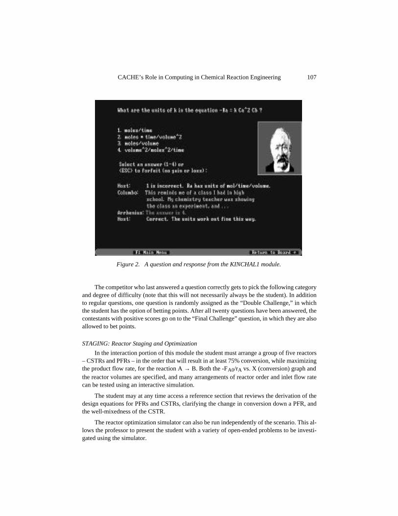
KINCHAL1: Kinetics Challenge 1 - Introduction to Kinetics
This module allows the students to test their knowledge of the general mole balance equa-tion and reaction rate laws, as well as types of reactions and reactors. The interaction occurs inthe form of an interactive game (see Fig. 1) with timed responses and computer-generated com-petitors. Twenty questions are selected from a pool of approximately 100 multiple choice ques-tions (see Fig. 2). Students can choose questions from any of four categories (mole balance,reactions, rate laws, and reactor types) and five difficulty levels (100 - 500 points):
The student has one minute to choose the correct answer. The module responds to the stu-dent’s choice, either reinforcing the reasoning for a correct answer, or immediately clarifyinga misunderstanding if an incorrect answer is entered. If no response is entered within the timelimit, or if an incorrect response is entered, the points are lost and one of the computer compet-itors tries to answer the question.
Figure 1. Choosing a category in the KINCHAL1 module.
CACHE’s Role in Computing in Chemical Reaction Engineering 107
The competitor who last answered a question correctly gets to pick the following categoryand degree of difficulty (note that this will not necessarily always be the student). In additionto regular questions, one question is randomly assigned as the “Double Challenge,” in whichthe student has the option of betting points. After all twenty questions have been answered, thecontestants with positive scores go on to the “Final Challenge” question, in which they are alsoallowed to bet points.
STAGING: Reactor Staging and Optimization
In the interaction portion of this module the student must arrange a group of five reactors– CSTRs and PFRs – in the order that will result in at least 75% conversion, while maximizingthe product flow rate, for the reaction A → B. Both the -FA0/rA vs. X (conversion) graph andthe reactor volumes are specified, and many arrangements of reactor order and inlet flow ratecan be tested using an interactive simulation.
The student may at any time access a reference section that reviews the derivation of thedesign equations for PFRs and CSTRs, clarifying the change in conversion down a PFR, andthe well-mixedness of the CSTR.
The reactor optimization simulator can also be run independently of the scenario. This al-lows the professor to present the student with a variety of open-ended problems to be investi-gated using the simulator.
Figure 2. A question and response from the KINCHAL1 module.

108 COMPUTERS IN CHEMICAL ENGINEERING EDUCATION
KINCHAL2: Kinetics Challenge 2 - Stoichiometry and Rate Laws
This module focuses on rate laws and stoichiometry, allowing the student to master theelements of the stoichiometric table. The interactive portion of the module is similar to that inKinetic Challenge 1. Students can choose from four categories (reactants, products, rate law,potpourri) and four levels of difficulty (200-1,000 points).
The key focus in this module is to provide students with practice so that they will avoidthe more prevalent mistakes (expressing the reaction rate law for an irreversible reaction as ifit were reversible, and using the ideal gas law for liquid-phase reactions).
COLUMBO: CSTR-Volume Algorithm - A Murder Mystery
The principal purpose of this module is to allow students to practice the algorithm forCSTR design.
In the interactive portion of the module the student must solve a murder mystery, with theaid of Lieutenant Columbo. It seems that overnight there was a slight irregularity in the con-version in the reactor at the Nutmega company (see Fig. 4).
It is feared that one of the employees may have been murdered by a fellow employee, andthe body left in the reactor. By analyzing the conversion data and using personnel informationand knowledge of CSTR reactor design, the student must determine the identity of both themurderer and the victim. Help may be obtained by questioning the suspects.
Figure 3. Frame from the COLUMBO module.

CACHE’s Role in Computing in Chemical Reaction Engineering 109
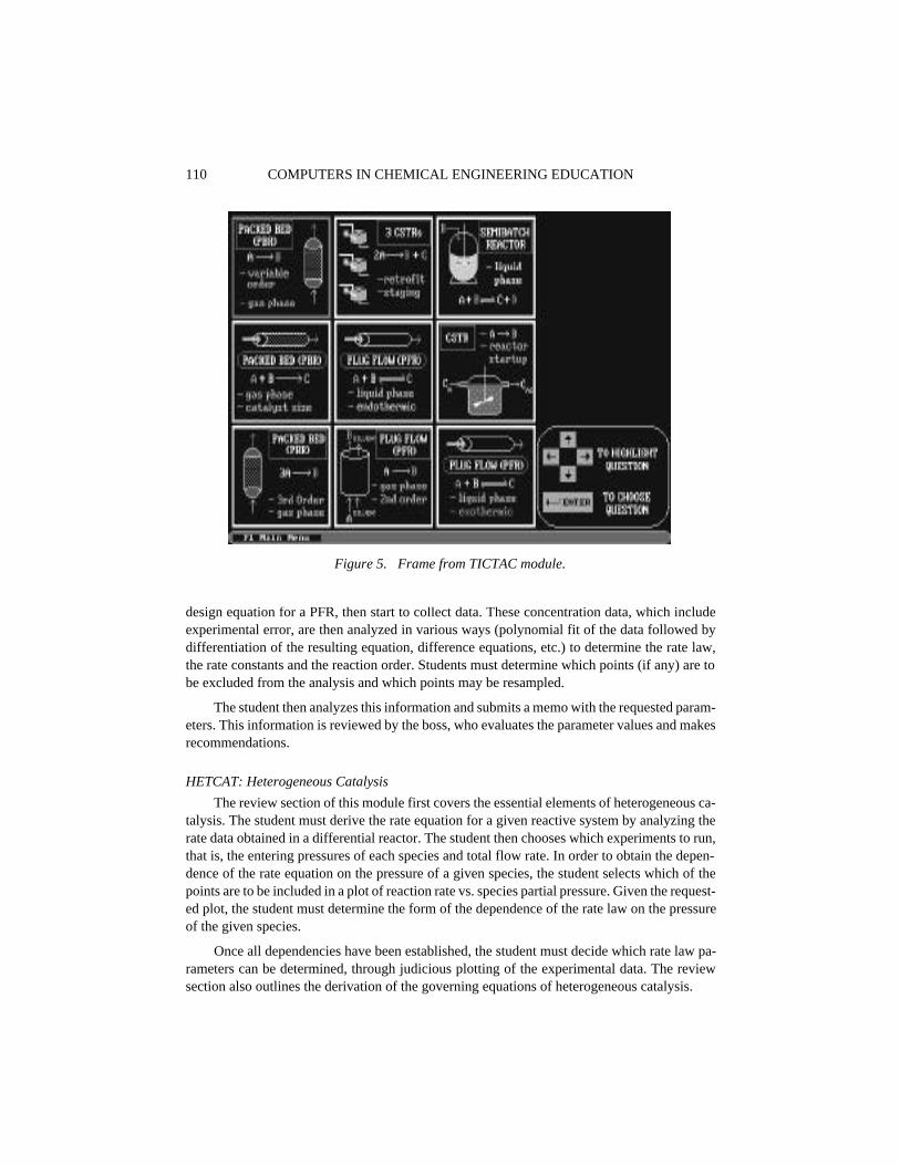
TICTAC: Ergun, Arrhenius, and Van’t Hoff Equations in Isothermal Reactor Design
This module allows the student to examine nine reactor design problems, and investigatethe effect of varying reactor parameters on process performance. The problems are organizedas in a tic-tac-toe board (see Fig. 5). The reactors covered by these problems include PFRs,CSTRs, packed bed reactors and semi-batch reactors.
The student must master the concepts in enough squares (three adjacent squares horizon-tally, vertically, or diagonally) to successfully win the tic-tac-toe game. Each problem allowsthe student the opportunity to examine the effect of a specified operational parameter on reactorperformance, using simulators:
After performing the “experiments,” the student proceeds to answer three questions thatexamine the effects observed. These effects can be explained through the Ergun, Arrhenius,and Van’t Hoff equations. In many cases, competing effects are highlighted. The square is“won” by answering two out of the three questions correctly.
ECOLOGY: Collection and Analysis of Rate Data - Ecological Engineering
The student, as an employee of a company trying to meet environmental regulatory agen-cy standards, must sample concentration data for a toxic material found in a wetlands channelbetween a chemical plant upstream and a protected waterway downstream, and analyze the rateof decay of the toxic material.
The wetlands are modeled as a PFR. The student must first develop the necessary reactor
Figure 4. Frame from the COLUMBO module.
110 COMPUTERS IN CHEMICAL ENGINEERING EDUCATION
design equation for a PFR, then start to collect data. These concentration data, which includeexperimental error, are then analyzed in various ways (polynomial fit of the data followed bydifferentiation of the resulting equation, difference equations, etc.) to determine the rate law,the rate constants and the reaction order. Students must determine which points (if any) are tobe excluded from the analysis and which points may be resampled.
The student then analyzes this information and submits a memo with the requested param-eters. This information is reviewed by the boss, who evaluates the parameter values and makesrecommendations.
HETCAT: Heterogeneous Catalysis
The review section of this module first covers the essential elements of heterogeneous ca-talysis. The student must derive the rate equation for a given reactive system by analyzing therate data obtained in a differential reactor. The student then chooses which experiments to run,that is, the entering pressures of each species and total flow rate. In order to obtain the depen-dence of the rate equation on the pressure of a given species, the student selects which of thepoints are to be included in a plot of reaction rate vs. species partial pressure. Given the request-ed plot, the student must determine the form of the dependence of the rate law on the pressureof the given species.
Once all dependencies have been established, the student must decide which rate law pa-rameters can be determined, through judicious plotting of the experimental data. The reviewsection also outlines the derivation of the governing equations of heterogeneous catalysis.
Figure 5. Frame from TICTAC module.

CACHE’s Role in Computing in Chemical Reaction Engineering 111
HEATFX-1: Simulation - Mole and Energy Balances in a CSTR
This module allows students to investigate the effect of parameter variation on the opera-tion of a non-isothermal CSTR. An extensive review section derives the energy balance for theCSTR, and also describes the terms in the mole balance that are temperature dependent.
A simulator is included in the review section. This allows the student to vary parametersand observe the effects on the conversion-temperature relationships (see Fig. 6) as describedby both the mole balance and the energy balance. The parameters that may be varied includefeed flow rate and temperature, the reversibility/irreversibility of the reaction, heat of reaction,heat exchanger area, and heat transfer fluid temperature. The operating conditions can be de-termined from the intersections of the mole balance and energy balance curves.
The module can also be run in the interactive mode, in which the scenario takes the studentto a basketball tournament. The student has the choice of two-point and three-point questions.The simulator is available to help in answering the three-point questions.
HEATFX-2: Simulation - Mole and Energy Balances in a PFR
This simulation allows the student to explore the effects of various parameters on the per-formance of a non-isothermal plug flow reactor. The student may choose from eight simula-tions, that span all combinations of exothermic/endothermic, reversible/irreversible conditions,as well as one simulation that includes the effect of pressure drop. The parameters that may bevaried include heat transfer coefficient, inlet reactant and diluent flow rate, inlet temperature,and ambient temperature.
Figure 6. Frame from the HEATFX-1 module.

112 COMPUTERS IN CHEMICAL ENGINEERING EDUCATION
The results from the simulator may be analyzed in the form of plots of concentration, con-version or temperature (see Fig. 7) as functions of reactor volume. The module may also be runin the interactive mode, in which the student must achieve specific goals (e.g., achieve a givenconversion without exceeding a given temperature within the reactor), in order to get to the cen-ter of the reactor complex.
Each interactive module has the following format:
• Menu
• Review of engineering principles
• Demonstration
• Interactive simulation
• Evaluation
In August of 1993, these interactive modules were sent by the CACHE Corporation to ev-ery chemical engineering department in the U.S. and to departments in foreign countries thatare CACHE subscribers.
A Paradigm Shift
With the emergence of extremely user-friendly software packages, students can exploreproblem solutions much more effectively, to develop an intuitive feeling for the reactor/reac-tion behavior, and obtain more practice in creative problem solving.
Figure 7. Frame from the HEATFX-2 module.

CACHE’s Role in Computing in Chemical Reaction Engineering 113
One of the most user friendly ODE solvers is POLYMATH, developed by ProfessorsMichael Cutlip of the University of Connecticut and Mordechai Shacham of Ben Gurion Uni-versity (Shacham and Cutlip, 1981a, 1981b, 1982, 1983). CACHE provided partial develop-ment support for the program and currently licenses POLYMATH to the industrial anduniversity communities.
The numerical package developed by Cutlip and Shacham had its origins in a computer-based course on chemical reaction engineering using the PLATO (Programmed Logic for Au-tomated Teaching Operations) System. This course, first offered in the late 1970s, was self-paced and had the following components:
• Self-Paced textbook (Fogler) 40%
• Homework assignments (on PLATO) 15%
• PLATO lessons 15%
• Videotape lectures 15%
• Reaction modeling and simulation (on PLATO) 7%
• Exams (on PLATO) 8%
This course was very successful when offered at both the University of Connecticut andthe University of Michigan. As material on reaction engineering for the individual lessons be-came sufficiently developed, Professors Cutlip and Shacham focused their efforts on develop-ing a numerical package that could be used with the course. Specifically, they begandeveloping software to solve the non-linear ordinary differential equations typical of thosefound in chemical reaction engineering when heat effects are important. In addition to theseODE solvers, data analysis and polynomial fitting routines were developed for use in thecourse. These numerical packages were the origins of the current version of POLYMATH.
Unfortunately, the course that was developed for the PLATO system ceased to exist in themid-1980s when support for it was withdrawn by its commercial supported. Fortunately, Pro-fessors Cutlip and Shacham were able to transport POLYMATH software from PLATO toIBM PCs. As a result, POLYMATH is now widely used throughout the US, Canada, Asia and
Figure 8. Paradigm shifts in chemical engineering education.

114 COMPUTERS IN CHEMICAL ENGINEERING EDUCATION
Europe. With POLYMATH, tedious and time consuming computer programming is eliminat-ed, and the reaction engineering student can explore complex problems by varying the param-eters and the operating conditions. Consequently, virtually every problem or homeworkassignment in chemical reaction engineering can be turned into an open-ended problem thatwill allow the students to practice their creative modeling and synthesis skills.
To illustrate this point, consider a gas phase exothermic reaction
A → B + C
carried out in a plug flow reactor with heat exchange.
For non-isothermal reaction in CRE we must choose which form of the energy balance touse (e.g., PFR, CSTR) and which terms to eliminate (e.g., Q=0 for adiabatic operation). Thestructure introduced to study these reactors builds on the isothermal algorithm by introducing
the Arrhenius equation, and k = A e-E/RT in the rate law step, which results in one equation withtwo unknowns, X (conversion) and T (temperature), when we finish with the combine step(Reilly, 1972). For example, using the PFR mole balance and conditions, we have, for constantpressure:
We now recognize the necessity of performing an energy balance on the reactor to obtain a sec-ond equation relating X (conversion) and T (temperature). An energy balance on a PFR withheat exchange yields the second equation we need, relating the independent variables X and T:
These simultaneous differential equations can be solved readily with an ODE solver, as dis-cussed below.
Obtaining the temperature and concentration profiles requires the solution of two couplednon-linear differential equations such as those given by Equations (1) and (2). In the past itwould have been necessary to spend a significant amount of time choosing an integrationscheme and then writing and developing a computer program before any results could be ob-tained. With the available software programs, especially POLYMATH, it rarely takes morethan 10 minutes to type in the equations and obtain a solution (Sacham and Cutlip, 1982). Asa result, the majority of the time for the exercise can be spent exploring the problem throughparameter variation and analysis of the corresponding observations. For example, in the aboveexothermic reaction in a PFR with heat exchange the students can vary such parameters as theambient and entering temperatures, the flow rates, and the heat transfer coefficient and look forconditions where the reaction will “ignite” and conditions for which it will “run away.” By try-ing their own different combinations and schemes, the students are able to carry out open-end-ed exercises that allow them to practice their creativity and better understand the physicalcharacteristics of the system.
dX
dV=
A e− E / R T1− X( )uo 1 + eX( )
To
T
(1)
dT
dV=
UAc Ta − T( ) + rA( ) ∆H R( )[ ]FA 0 CPA
(2)

CACHE’s Role in Computing in Chemical Reaction Engineering 115
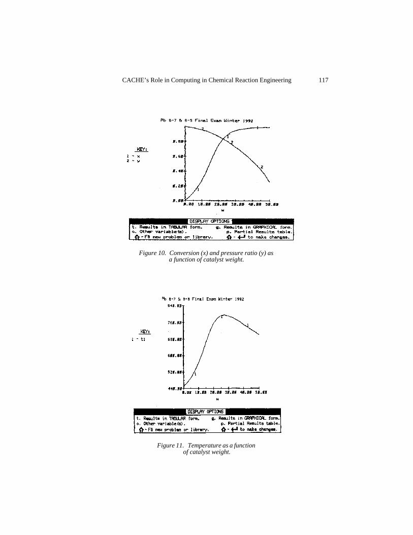
The following example, which was given as 50% of a 2 hour final exam at the Universityof Michigan, illustrates how significantly more complex problems can be rapidly solved withPOLYMATH.
The elementary irreversible gas exothermic phase reaction
A → 2B
is carried out in a packed bed reactor. There is pressure drop in the reactor and the pressure drop
coefficient is 0.007 kg-1. Pure A enters the reactor at a flow rate of 5 mol/s, at a concentrationof 0.25 mol/dm3, a temperature of 450 K and a pressure of 9.22 atm. Heat is removed by a heatexchanger jacketing the reactor. The coolant flow rate in the jacket is sufficient to maintainthe ambient temperature of the heat exchanger at 27°C. The maximum weight of catalyst thatcan be packed in this reactor is 50 kg. The term giving the product of the heat transfer coeffi-cient and area per unit volume divided by the bulk catalyst density is given by:
a) Plot the temperature, conversion X, and the pressure ratio (y = P/P0) as a function of catalystweight. b) At what catalyst weight down the reactor does the rate of reaction (-rA) reach itsmaximum value? c) At what catalyst weight down the reactor does the temperature reach itsmaximum value? d) What happens when the heat transfer coefficient is doubled? e) What hap-pens if the heat coefficient is halved? f) Discuss your observations of the effects on reactor per-formance (i.e., conversion, temperature and pressure drop).
Additional Information:
∆HR = -20,000 J/mol A at 273 K, CPA = 40 J/mol K, CPB = 20 J/mol K, E = 31.4 kJ/mol, and
Ua
ρB
=
5 Joule
kg cat ⋅s K(3)
k = 0.35 expE
R
1
450−
1
T
dm3
kg.cat.sec(4)
116 COMPUTERS IN CHEMICAL ENGINEERING EDUCATION
The relevant equations are:
The POLYMATH solutions for this problem are shown in Figs. 9-12.
dXdW
= − ′ r A / F A0
dPdW
= −α2
TT0
P0
(P / P0 )1+ εX( ) or
dydW
= −α2
TT0
1 + εX( )y
dT
dW=
U a
P BTa − T( ) + − ′ r A( ) −∆Hr( )
FA0 CP A+ X 2CPB
− CP A( )( )
− r A = k CA
CA = CA0
1− X( )1+ X( )
T0
T
P
P 0
k = 0 . 3 5 e x p 3776.76 1
450−
1
T
Figure 9. POLYMATH equations.
CACHE’s Role in Computing in Chemical Reaction Engineering 117
Figure 10. Conversion (x) and pressure ratio (y) as a function of catalyst weight.
Figure 11. Temperature as a function of catalyst weight.

118 COMPUTERS IN CHEMICAL ENGINEERING EDUCATION
The Purdue-CACHE Modules
The Purdue-Industry Computer Simulation Modules are another educational innovationthat CACHE fostered through Task Force support and distribution to virtually all chemical en-gineering departments in the US and Canada. Since 1986, a series of computer modules ofstate-of-the-art chemical engineering industrial processes have been and are being developedat Purdue University (Squire et al., 1992, Anderson et al., 1992). Each module has an industrialsponsor who furnishes data on a process on which the simulation is based and also produces a20 minute videotaped “tour” of the real process. A number of these modules focus on chemicalreaction engineering.
The modules are meant to supplement, not to replace, traditional laboratory experiments.Computer-simulated experiments have a number of advantages over traditional experiments:
• Processes that are too large, complex, or hazardous for the university labo-ratory can be simulated with ease on the computer.
• Realistic time and budget constraints can be built into the simulation, givingstudents a taste of “real world” engineering problems.
• The emphasis of the laboratory can be shifted from the details of operatinga particular piece of laboratory equipment to more general considerations ofproper experimental design and data analysis.
• Computer simulation is relatively inexpensive compared to the cost ofbuilding and maintaining complex experimental equipment.
• Simulated experiments take up no laboratory space and are able to servelarge classes because the same computer can run many different simula-tions.
Figure 12. Reaction rate as a function of catalyst weight.

CACHE’s Role in Computing in Chemical Reaction Engineering 119
Each module is written as an industrial problem caused by a change of conditions in anexisting process, requiring an experimental study to re-evaluate the characteristic constants ofthe process. These might include, for example, reaction rate constants, equilibrium constants,heat transfer and mass transfer coefficients, and phase equilibrium constants. The studentteams are expected to design experiments that will enable them to evaluate the needed con-stants. This is referred to as the measurements section of the problem.
After the constants have been determined, the students must validate them by using themin an existing computer model of the process, and comparing the simulated and experimentalresults. When they are convinced that their constants are reliable, the students must use theseconstants to predict some other specific process performance characteristics. This is called theapplications section.
Each process is made to seem realistic not just by the videotaped “tour” but also by theassigned financial budget and time constraints. The problems are open-ended in that the exper-imental conditions such as temperature, pressure, flow rates, and compositions are under thestudent’s control. The cost and the associated duration of running experiments vary with thetype of experiment and are also functions of operating conditions. Instructor-controlled statis-tical fluctuations are built into the simulations so that the results of duplicate experiments arenot identical. The students must plan their experiments to obtain data from which, with properanalysis, the required constants may be determined without exceeding their budgetary and timeconstraints.
In the Purdue course, students work in teams of three and have eight 3-hour classes tocomplete the assignment. After an introductory 2-hour lecture, they are on their own. If theyhave queries, they are free to ask the consultant (the instructor, of course), but are charged a feewhich is deducted from their budget. Written reports and a 20-minute oral presentation (videorecorded for later analysis by the instructor and the student) are required.
Chemical kinetics has played a large role in most of the modules. The following sectiongives a brief outline of the chemical kinetics application of each of the Purdue modules.
Amoco Resid Hydrotreater (Squires et al., 1991)
This module requires the students to design a series of experiments (in a pilot plant, usingone, two, or three CSTR’s in series) to determine the rate constants of a series-parallel networkof seven pseudo-first-order non-catalytic irreversible reactions. In addition, the rate constantsmust be determined for the catalytic desulfurization reaction, which follows Langmuir-Hin-schelwood kinetics. This study is complicated by the fact that the catalytic activity deactivateswith time.
Once the constants have been determined, the students are asked to start up the plant. Thisis complicated, since the reaction network is unstable with multiple steady-state solutions.Non-optimal control strategies may easily lead to temperature runaways.
Dow Styrene-butadiene Copolymerization (Jayakumar et al., 1995)
The students must determine the rate constants of the four propagation reactions and twochain transfer reactions, by designing experiments to be run in a two-gallon laboratory reactor.

120 COMPUTERS IN CHEMICAL ENGINEERING EDUCATION
Once the constants are determined, students are asked to predict the performance of a10,000 gallon plant reactor. This is complicated, since the reactor has insufficient surface areafor heat transfer. Students must determine:
a. how much additional heat transfer surface area is needed, or
b. the amount of feed pre-cooling required to achieve controllability.
Mobil Catalytic Reforming (Jayakumar et al., 1994)
In this study, the process is simplified by considering the catalytic reforming of only theC6 range of hydrocarbons. The students must determine the catalyst deactivation parameter ofa series of four coupled reforming reactions.
Once the parameters are known, students are asked to predict the hydrogen-to-hydrocar-bon ratio in the feed that will optimize the annual profit of the process.
Eastman Chemical Reactive Distillation (Jayakunmar et al., 1993)
One step in Eastman Chemicals acetic anhydride from coal process, involves the sulfuricacid catalyzed reaction:
acetic acid + methanol → methylacetate + water
This reaction is normally equilibrium limited. The key concept of the reactive distillation pro-cess relies on methylacetate being more volatile than the other reactants and products. The re-action occurs on a distillation tray, and a significant amount of methylacetate will vaporize,forcing the reaction to the right and increasing the yield beyond the normal equilibrium limita-tion.
Air Products Hydrogen Reactive Cooling Process
Hydrogen at room temperature is an equilibrium mixture of 25% para and 75% ortho.When cooled below 30˚R the equilibrium mixture is almost 100% para-hydrogen. If the hydro-gen is cooled in the absence of a catalyst, the ortho-para reaction will not take place and theresulting liquid hydrogen will still be 75% ortho. In the liquid hydrogen storage vessel theortho-para reaction will occur, and the exothermic heat of this reaction will cause the vaporiza-tion of much of the liquid hydrogen.
In order to avoid the boil-off losses, it is necessary to catalyze the ortho-para hydrogenreaction during the cooling process rather than later in the storage vessel. The students mustdetermine the rate constants for the ortho-para reaction.
Once the constants are determined, the students are asked to determine the optimum num-ber of side reactors required for the reactive cooler design.
Concluding Comments
In July 1990, and again in July 1991, three-day workshops were held at Purdue Universityat which the chemical engineering faculty participants were given hands-on experience with allthe modules. Faculty representatives from 56 chemical engineering departments in the United

CACHE’s Role in Computing in Chemical Reaction Engineering 121
States and Canada participated in these workshops. Many of these schools are now using someof the modules. It is particularly interesting to note that several of the other schools (notablyGeorgia Tech., Carnegie Mellon, West Virginia) are using the materials as problems in reactordesign courses. The authors also presented a workshop on the project at the ASEE ChemicalEngineering Faculty Summer School in August 1992. The modules are currently being used by25 schools, including five schools in foreign countries.
The modules were originally created for execution on Sun (UNIX) workstations. NSF hasrecently funded a proposal to port the modules to other workstations (such as DEC, IBM, HP,and Silicon Graphics). Nine other schools have agreed to participate as beta-test sites in thiswork, bringing the total number of user schools to 34. Once the modules are available on theseother computers, there should be a significant increase in the number of participating schools
The University Of Washington – CACHE Project
The Chemical Reactor Design Tool is a set of computer programs that permit a student todesign chemical reactors, including the realistic transport effects that are frequently present.The interface is written in X-windows so that the student can include complications easily; theprogram automatically uses the correct, robust tools to solve the problem. Results are displayedgraphically, which makes comparison studies especially easy. The programs were developedby Professor Bruce Finlayson under sponsorship of the National Science Foundation and theUniversity of Washington, and are made available to universities through CACHE.
CRDT Educational Goals
Introductory textbooks concentrate on problems that can be solved analytically. Recenttextbooks include material for problems that can be solved with an ordinary differential inte-grator. These include batch reactors and simple plug flow reactors; extensions from one reac-tion to several reactions are possible, but time-consuming. When attempting to solve realproblems, students are faced with several difficulties, which are mostly difficulties in manipu-lation and book-keeping rather than conceptual. Phenomena that might be important include:
• Multiple reactions (lots of bookkeeping)
• Temperature of catalyst and fluid may be different
• There may be internal mass transfer (requires solving an effectiveness factorproblem)
• There may be cooling at the wall (leads to radial dispersion)
Students and design engineers may not be able to make realistic estimates of which phe-nomena must be included. In some cases it is necessary to calculate with a suspected phenom-enon included to see if it is important. That has been difficult to do, because each phenomenoncreates problems that require special techniques to solve. Used in the CRDT are ordinary dif-ferential equation integrators, the orthogonal collocation method, the finite difference method,techniques to convert partial differential equations to sets of ordinary differential equations, it-erative techniques to solve large sets on nonlinear equations, and linear programming methodsto guide initial guesses for integrative techniques. All these methods are transparent to the user.
122 COMPUTERS IN CHEMICAL ENGINEERING EDUCATION
Key Aspects
The user can examine effects very easily and make their own deductions about the impor-tance of physical phenomena. Phenomena that can be easily included are:
• Different reactors: CSTR, batch, plug flow
• Axial dispersion, radial dispersion
• Intraparticle heat and mass transfer
• Significant mole changes
• Significant pressure changes
The cases when it makes a difference are:
• Selectivity, especially in non-isothermal cases
• Non-isothermal problems
None of these complications is too complicated for the student to do, but there is not enoughtime to do so. In design problems, though, some of these complications are necessary.
Textbook Supplements
An important feature is the Textbook Supplement, which gives any new equations in thenotation of that textbook. Since the programs are much more general than can be treated inmost undergraduate books, it is necessary to explain the problems continuing the notation ofthe textbook being used by the student. In addition, a two-page handout provides hints on thebest way to approach problems, summaries of the equations for easy reference, and standardcorrelations for some of the transport properties. This handout is designed for quick referencewhile using the program.
Design Decisions
Design decisions may revolve around conflicting constraints, none of which can be easilyhandled if one has to write the program:
• Use a small catalyst diameter to avoid diffusion resistance; but this increases thepressure drop.
• A recycle compressor may be an expensive component in a gas-phase reaction sys-tem.
• An adiabatic reactor avoids radial dispersion, but the temperatures may betoo big; cooling at the wall usually makes radial dispersion important.
By using the Chemical Reactor Design Tool these realistic complications can be treated by thestudent-designer.
Output
Output is presented graphically in addition to printed form. The user can call for the fol-lowing plots:

CACHE’s Role in Computing in Chemical Reaction Engineering 123
• line plots
• 3D perspective views
• 2D contour plots
• solution variables: concentration, molar flow rate, temperature wall flux
• each term in the equations: diffusion, reaction, convection terms
These plots are created automatically, but the user has some control over them either be-fore they are created (contour and 3D views) or after they are created (line plots).
Conclusions
What will the next 25 years bring? We are already beginning to see the development ofmultimedia modules with the newest CACHE/NSF/University of Michigan initiative under thedirection of Professor Susan Montgomery. Part of this project will involve development of ki-netic and bioreactor modules which will incorporate video-clips showing growing bacteria aswell as the transport of bacteria in porous media.
Another exciting area on the horizon is virtual reality (VR). CACHE has recently formeda Virtual Reality Task Force; within the next five years we will see a significant number of VRmodules developed. One module currently under simultaneous development and testing at theUniversity of Michigan is the prototype of a chemical plant that uses a straight-through trans-port reactor with a coking catalyst. Here the student uses VR to enter the plant lobby where heor she is given an overview of the process and is free to explore various parts of the room andvideo tapes at will, simply by moving a joy stick. After this introduction, the student enters thereactor room where he or she can change the operating parameters and see their effect on thereaction variables such as degree of coking, conversion, etc. The student can enter the reactorto observe the coking and catalyst transport, and, in addition, can enter the catalyst pellet toview the internal pore space and reactions occurring on the surface. This visualization of theprocess and reaction mechanisms will greatly enhance the students’ understanding and appre-ciation of this reaction engineering process.
In addition to POLYMATH, the use of other software packages is on the rise in CREcourses. MATLAB, MAPLE, and Mathematica are becoming increasing user friendly and alsoare now being introduced in the freshman calculus or required computing courses at many uni-versities. These packages will provide greater flexibility and a higher level of sophistication inthe type and degree of complexity of problems the students can solve. In addition to these ODEsolvers, we can expect partial differential equation (PDE) solvers to be available in the not toodistant future. The PDE solvers will allow the students to explore radial as well as longitudinalgradients in packed bed reactors.
Finally, we can expect our future textbooks to be on CD-ROMs, so that the student caninteract with the book while reading it. Interactions will include video-clips, audio, animationof mechanisms and equations, and much more. The CACHE CD-ROM task force has alreadyprepared and distributed two CD-ROMS containing many instructional modules, video-clips,POLYMATH, and early versions of some of the papers in this monograph. There are great ex-citements ahead in computing in chemical reaction engineering.

124 COMPUTERS IN CHEMICAL ENGINEERING EDUCATION
References
Andersen, P.K., S. Jayakumar, R. G. Squires, and G.V. Reklaitis (1992). Computer Simulations in Chemical En-gineering Education. Proceedings on Frontiers in Education Conference, Nashville, TN.
Fogler, H.S, S.M. Montgomery, and R.P. Zipp (1992). Interactive Computer Modules for Undergraduate Chem-ical Engineering Instruction. Computer Applications in Engineering Education, 1, 11-24.
Jayakumar, S., R.G. Squires, G.V. Reklaitis, P.K. Andersen, and L.R. Partin (1993). Purdue-Industry ChemicalEngineering Laboratory Computer Module-II. Eastman Chemical Reactive Distillation Process. Chemi-cal Engineering Education. 27(2), 136-139.
Jayakumar, S., R.G. Squires, G.V. Reklaitis, P.K. Andersen, B.C. Choi, and K.R. Graziani (1994). The Use ofComputer Simulations in Engineering Capstone Courses: A Chemical Engineering Example–The MobilCatalytic Reforming Process Simulation. International Journal Engineering Education, 9(3), 243-250.
Jayakumar, S., R.G. Squires, G.V. Reklaitis, P.K. Andersen, and B.K. Dietrich (1995). The Purdue-Dow Styrene-Butadiene Polymerization Simulation.Journal of Engineering Education, 84(3), 271-278.
Reilly, M.J. (1972). Computer Programs for Chemical Engineering Education: Volume II - KINETICS, CACHE,Houston, TX.
Shacham, M. and M.B. Cutlip (1981). Computer-Based Instruction: Is There a Future in ChE Education? Chem-ical Engineering Education, 78.
Shacham, M. and M.B. Cutlip (1981). Educational Utilization of PLATO in Chemical Reaction Engineering.Computers & Chemical Engineering. 5(4), 215-224.
Shacham, M. and M.B. Cutlip (1982). A Simulation Package for the PLATO Educational Computer System,Computers & Chemical Engineering, 6(3), 209-218.
Shacham, M. and M.B. Cutlip (1983). Chemical Reactor Simulation and Analysis at an Interactive Graphical Ter-minal. Modeling and Simulation in Engineering, 27.
Squires, R.G., G.V. Reklaitis, N.C. Yeh, J.F. Mosby, I.A. Karimi, and P.K. Andersen (1991). Purdue-IndustryComputer Simulation Modules–The Amoco Resid Hydrotreater Process. Chemical Engineering Edition.32, 98-101.
Squires, R.G., P.K. Andersen, G.V. Reklaitis, S. Jayakumar, and D.S. Carmichael (1992). Multi-Media Based Ed-ucation Applications of Computer Simulations of Chemical Engineering Processes. CAEE, 1(1).

125
TRANSPORT PHENOMENA
Bruce A. FinlaysonUniversity of Washington
Seattle, Washington 98195
Andrew N. HrymakMcMaster University
Hamilton, Ontario L8S 4L7 Canada
Abstract
This chapter describes computer software that is available for solving transport prob-lems, including those with fluid flow. Included are programs that run on PCs, programsthat need workstations, and commercial codes that run on large workstations. All pro-grams described here were generated in the 1980s and 1990s.
Introduction
Chemical engineering education was revolutionized in the 1960s by the introduction oftransport phenomena, as advanced originally by the seminal book
Transport Phenomena
, byBird, Stewart and Lightfoot (1960). The subject requires more mathematics than other parts ofthe curriculum, and typical transport courses invoke heavy use of mathematics. Because math-ematics in the 1960s was mostly done analytically, problems treated in transport courses havefocused on problems that are simple enough to be solved analytically. Usually that means theproblems are one-dimensional and linear, e.g., fully developed flow in a pipe. When flow oc-curs it is usually laminar. Situations involving two dimensional flows or turbulent flows are nothandled except in extremely simple cases, e.g., flow past a sphere at zero Reynolds number, orwith correlations, e.g., Nu = f(Re, Pr).
With modern numerical tools it is possible to solve more realistic models. Thus the studentmust be able to formulate the problem in a reasonable way. In fact, industrially the problemmay be solved by a packaged program, or a program written by a computer scientist. Thus theformulation of the problem, and the need to verify and understand assumptions, is especiallyimportant as we look into the future. Of all the areas in the curriculum, transport phenomena isprobably the one that has been influenced least by the growth of computer power; it thus standsto gain the most by the introduction of computer tools.
In the 1980s CACHE established a task force to develop IBM PC lessons for chemical en-gineering courses other than design and control. This task force was under the chairmanship ofProfessor Warren Seider of the University of Pennsylvania and developed a number of modules
126 COMPUTERS IN CHEMICAL ENGINEERING EDUCATION
which were distributed to all Universities supporting CACHE. Only one of the lessons in-volved transport - design of a slurry pipeline, and it is described below. Throughout the 1980sthe CACHE News ran a column announcing programs written by professors, edited by Profes-sor Bruce Finlayson of the University of Washington. Only one of those programs falls into theclass of a transport program - solving the convective diffusion equation in one-dimension andtime, and it, too, is described below. A CACHE task force was formed to develop specific les-sons for the IBM PC that could be used in transport courses. Most of these were eventuallyabandoned, it is very time-consuming to generate a decent computer lesson! However, Profes-sor Scott Fogler at the University of Michigan persisted and developed several modules thatare described below. Finally the use of spreadsheets can be advantageously applied to transportproblems, and Professor Finlayson described those in a chapter in the second edition of a trans-port book by Professor Ray Fahien (1995) of the University of Florida. A brief summary ofwhat can be done is provided here.
When looking to the future, an on-going project is described that makes available finiteelement tools to seniors to solve transport problems that are extensions of those in their texts.This is an advanced topic that may be most relevant to senior students and beginning graduatestudents. Described here is the philosophy of the Transport Module being prepared by Profes-sor Finlayson, and then a review of commercial computational fluid dynamics codes is givenfor those that have access to them.
PC Programs
Design of a Slurry Pipeline
The slurry pipeline computer program was written by William Provine, Benny Feeman,Gregory Dow, and Professor Morton Denn at the University of California at Berkeley. The em-phasis was to provide a design problem that students could solve using the theory and under-standing they had achieved in their fluid mechanics course. The problem is to design a slurrypipeline for transporting material under specified conditions. The students can choose to diluteit, to reduce its viscosity, operate it in laminar or turbulent flow, and must avoid settling of thesuspended solids. Simplifications are made - a maximum pressure is specified so that the costfactors involved in thicker pipe walls need not be included, the suspension exhibits no yieldstress and no shear rate dependence - but the essential part of the problem remains. Economicdata are supplied, along with a program to do some of the technical calculations.
The basic equations are
for the slurry viscosity,
η = 98 ηSF
(φ / φs)1/3
1 − (φ / φs)1 /3
laminar: f = 16Re
turbulent: f = 0.046
Re0.2
Transport Phenomena 127
for the friction factor, and
for the minimum velocity for reentrainment of a sedimenting slurry. The problem statementthen leads the student through exercises establishing the minimum power for turbulent flow,for laminar flow, and for any flow. The computer program runs on an IBM compatible com-puter under the DOS operating system.
CDEQN
This program was written by Professor Bruce Finlayson to solve the transient convectivediffusion equation in one space dimension.
The methods used include the finite difference method and the Galerkin finite element methodand the solution is plotted automatically at various times. A variety of numerical choices areavailable to the student, so that they can explore how those choices affect their solution. Suchmatters are very important when they turn to simulations of the flow of contaminants under-ground, for example; improper use of the packaged programs can lead to misleading results.Later this program was expanded into a commercial program, CONVECT, which has manymore numerical methods. The program runs on a Macintosh computer with any operating sys-tem (although System 7 users must turn off the cache memory).
PC Lessons
A series of PC lessons has been developed at the University of Michigan under the direc-tion of Professor Scott Fogler. The program “Shell: Shell Momentum and Energy Balances”leads the student through the exercise of making shell balances for three problems: water flow-ing down a vertical flat surface, water flowing through a vertical circular tube, and heat con-duction in an electric wire. If the correct shell balance is achieved, the solution to the problemis displayed. The program “Simp: Simplification of the equations of motion and energy” workson the problem in the reverse order: the student chooses which terms to leave out of the equa-tions to simplify them to model one-dimensional transport. This module uses the language ofvideo games. It is called the “Equation Avenger,” and the student ‘shoots’ the unnecessaryterms. Since there seems to be a definite bias between boys and girls playing video games, andthe type of game they prefer, this module may run afoul of the Politically-Correct Police andbe inappropriate for the men and women in our classes! The program “Visc: Rheology - Iden-tification of Liquids” helps the student review viscometer principles for identifying the type ofnon-Newtonian fluid. “Patch: Diffusion - Drug Patch Design” requires the student to design adrug patch that supplies a drug to astronauts in a space shuttle mission. The drug flow rate mustfall within a specified range, and this flow rate must be maintained for a required amount oftime. The student can use the simulator to experiment with different materials (diffusivities),
vR = 1.3
2gD
ρS
ρSF − 1
1/2
∂c∂t + Pe
∂c∂x =
∂2c
∂x2

128 COMPUTERS IN CHEMICAL ENGINEERING EDUCATION
patch thicknesses, and different reservoir drug concentrations. Thus the student is exposed toopen-ended design problems in the transport course, which is a trend of growing importance.“Thermowell: Conduction, Convection and Radiation” allows students to investigate the ef-fects of various thermowell parameters on the temperatures measured by a thermocouple.Again the problem is open-ended and the computer allows students to try many choices easilyand quickly.
Transport Using Spreadsheets
Professor Bruce Finlayson at the University of Washington has written a chapter entitled“Numerical Methods for Solving Transport Problems” for the second edition of the book
Fun-damentals of Transport Phenomena
, by Ray W. Fahien, McGraw-Hill, New York (first edi-tion: 1983). This chapter describes methods for solving typical and extended transportproblems using the numerical tools that exist today.
The first section treats a heat transfer problem. First the problem is taken as a linear prob-lem, so that the finite difference method can be described. Then complications are added to theproblem: a thermal conductivity that depends on temperature and a heat generation rate that isnot constant. The equations solved are
Finally, the solution of these problems is described using a spreadsheet program with iterationcapabilities, and detailed information is given about how to organize the calculations and checkthem. The next section considers transient heat transfer.
The finite difference method is applied to reduce the problem to a set of ordinary differentialequations (using the method of lines), and packages such as MATLAB are used to solve them.The final section considers the more complicated situation of heat conduction in both direc-tions.
Such problems can be solved using iterative methods as long as the domain has straight edges(either constant x or constant y, but there can be many of them). A problem is worked showingthe effect of having a hole in the middle of the domain. The finite element method is also ap-plied to the same problem so that students can see the limitations of using a spreadsheet pro-gram for such problems.
When solving differential equations numerically, though, there are still approximationsmade, and the possible error must be assessed. Throughout the chapter methods are given fororganization of the calculations, often with solution of a simpler problem which is easily
1r
ddr
k r dTdr
= − 2 Φ0
k
1 −
r2
R2
k = k0 [ 1 + a (T − TR) ]
∂T*∂t = α
∂2T*
∂x2
∂2T
∂x2
+ ∂2T
∂y2 = 0 in 0 ≤ x ≤ 1, 0 ≤ y ≤ 1

Transport Phenomena 129
checked, and with complications introduced one by one with checking at each step. Of evenmore importance, though, is the use of the truncation error to determine the error of the numer-ical solution. Since the error in the solution is proportional to some power of
∆
x, for example,the solution values should follow that behavior when the problem is resolved with a different
∆
x. By using this information, it is possible to assess the accuracy of the numerical solution,and improve it if necessary (it seldom is).
Workstation Programs
Brief Description of Transport Module
The Transport Module is being developed by Professor Bruce Finlayson at the Universityof Washington to allow students to solve fluid mechanics and transport problems in laminartwo-dimensional flow situations. The program uses the finite element method to discretize themesh. The user sketches the domain on the screen, identifies the fixed boundaries, flow bound-aries, etc., sets the boundary conditions, and then instructs the program to solve the problem.The finite element mesh is constructed automatically, and the results are displayed graphicallyas contour plots. The user interface is constructed in X-windows for use on Unix machines.
Goals
With the Transport Module students will be able to investigate fluid flow phenomena,such as how vorticity is generated, convected and diffused, and how this influences the flowfield, heat and mass transfer. They will be able to make quantitative estimates - such as: “Is itisothermal?”, and “If not, how much error is introduced?” It is even possible that students cantackle design problems in their senior year that involve small-scale processes and transport lim-itations, including the interaction of flow, heat, and mass transport, such as might occur inchemical vapor deposition. As they solve problems under different assumptions, students willgain intuition rather than just make assumptions because the instructor says so, or because ofmathematical convenience. Examples can be more exciting and can involve the newer technol-ogies. A textbook supplement will provide problems that are tied to existing textbooks, makingit easy to incorporate the new ideas in existing courses.
Detailed Description of the Transport Module
The three pillars on which the Transport Module is built are the user interface (to specifythe problem), the finite element programs, and the graphics display of the results.
The user interface allows the user to sketch the domain as a series of lines or quadraticcurves. Boundary conditions are specified for each of these lines in a natural way. Whereasmost finite element codes allow you to specify each variable at each boundary node, this gen-erality can also lead to gross modeling errors. Thus students are restricted to choosing boundaryconditions that make sense: solid boundary, flow boundary, centerline (symmetric) boundary,etc. This restriction prevents gross errors, and it also makes the data entry considerably simpler.The fluid flow and heat transfer properties are easily entered in an X-windows interface.
The finite element codes allow a variety of problems to be solved, but are restricted tolaminar flow in two dimensions, either Cartesian or cylindrical geometry. The Navier-Stokes

130 COMPUTERS IN CHEMICAL ENGINEERING EDUCATION
equations can be solved, including the possibility of the viscosity depending on shear rate, sothat simple non-Newtonian fluids like power law and Bird-Carreau fluids can be modeled. Theenergy and transport equation can also be added, in which case the viscosity can depend ontemperature as well. The user specifies a viscosity subroutine and a heat generation and rate ofreaction term as well. The primary aim is to allow flow and heat transfer, rather than a completeinclusion of chemical reaction phenomena. Only one chemical species can be included, allow-ing for dilute systems or systems in which the number of moles does not change. Chemical re-actor models are best handled with the Chemical Reactor Design Tool. The energy equationcan be solved by itself for heat transfer problems, and the energy and mass transfer equationcan be solved with a specified velocity for chemical reactor situations.
Following solution of the finite element problem, various post-processing programs areinvoked to make the results more meaningful. First, vorticity and streamline are determined, ifdesired. Then various plotting options are chosen. The flow situation can be examined by plot-ting the steamlines and vorticity, but more detail is also available. The different terms in theequation can be plotted individually; thus the convective and the viscous terms can be com-pared for flow around a cylinder, and the student can explore the Stokes paradox. The stresscomponents can be plotted, as can the viscosity throughout the domain. Both of these plots areuseful for gaining insight to non-Newtonian flows. When the energy equation is solved, the vis-cous dissipation term can be plotted and compared with the diffusion or convection term; thishelps the student see the validity of the constant temperature approximation. These pictures areespecially meaningful when done in a 3D perspective view. In addition, certain properties canbe viewed along boundaries: the drag forces and heat flux.
Because of the processing power needed to run the finite element codes, the actual calcu-lations can best be done on a large computer, and the Unix environment makes this especiallyeasy. With the X-windows display on a local computer screen, the graphics can be viewed lo-cally (and printed locally), but the speed of the central processor is especially welcome. Ofcourse, calculations can be done at the workstation, too, but with more delay. When computerpower increases it will be possible to do the processing locally, too.
Of course it is necessary for educational purposes that the student be able to solve manyproblems they have seen before. Most of the problems they solved in transport are one-dimen-sional, but these can be solved in the Transport Module as well (with some loss of efficiency).Couette flow, Poiseuille flow, and combined Couette-Poiseuille flows are all solvable. TheGraetz problem can be solved with fully developed flow, with developing flow, with New-tonain and non-Newtonian fluids, and with temperature-dependent viscosity. Laminar bound-ary layer problems can be solved, as can flow past spheres and cylinders. The effect of wallsaround the spheres and cylinders can be explored, provided the geometry still retains a two-dimensional character.
In the time since the project was defined the power and availability of commercial codeshas increased (see below) to the point that this program may never be made available. Howev-er, the method of using them in class and interacting with the existing curriculum have valuethat is not provided by commercial codes. Such interactions are described below.

Transport Phenomena 131
Sample Questions which can be Explored
Consider any flow problem, e.g., flow past a sphere. What is the effect of Reynolds num-ber? How small is small, so the inertial effects can be ignored? How large is large, so the iner-tial effects must definitely be included? How big are the inertial terms (which one would liketo ignore) compared with the diffusion terms? These are questions which can be answered bystudents using the Transport Module. Once their intuition has been developed, the TransportModule can be used in more design-type situations. They can compare the effect of differentshapes (at least cylindrical shapes with different cross sections).
In the heat transfer problems the students can see the effect of Prandtl number, in that iteffects the boundary layer thickness, which they will see in the plots. They can allow the ther-mal conductivity to depend on temperature if they think that is important, and compare resultsto simulations in which the thermal conductivity is constant. The heat transfer module can alsobe used to solve Laplaces’s equation, making it suitable for some problems in electronic mate-rials processing. There the effect of different geometries can be easily explored.
Sample Extension Problems
Listed below are several problems of the kind that can extend those in current textbooks.The examples are some of those related to Denn’s book (1980), but textbook supplements caneasily be prepared for all major textbooks. For the Chemical Reactor Design Tool only twotextbooks supplements were prepared, because there are only two major books used by univer-sities, but the added work to prepare a second supplement is small compared to the work nec-essary to prepare the first one.
Flow of a sphere in a tube, p. 61. How far away does the outer boundary haveto be for less than 5% effect? Check the correlation in Figure 4-6. Extend thatcorrelation as a function of Reynolds number.
Flow past objects that are not regular, p. 66. Compare the drag of a sphere withthat of a disk oriented with the flat edge forward. Consider other shapes. Preparea universal graph (and test it) by using the surface to volume ratio to obtain aneffective diameter.
Calculate pressure drops in a reaction injection molding device, p. 136.
Flow in a manifold, p. 125. With one inlet and several outlets, how much flowgoes out each?
Determine the errors incurred when measuring the pressure at the bottom of ahole or slit.
Entrance pressure loss in contracting flows, p. 336. Correlate it, design a shapethat will minimize it, do for power law fluids, too.
Flow Distribution in a single screw extruder, p. 197. Do a two dimensional anal-ysis and determine the errors in the one dimensional analysis.
Boundary layer flow, p. 286. Do an complete analysis for flow past a flat plateand examine the terms that have been neglected in the boundary layer analysis.Are they really small? How small? How large a region is affected?
132 COMPUTERS IN CHEMICAL ENGINEERING EDUCATION
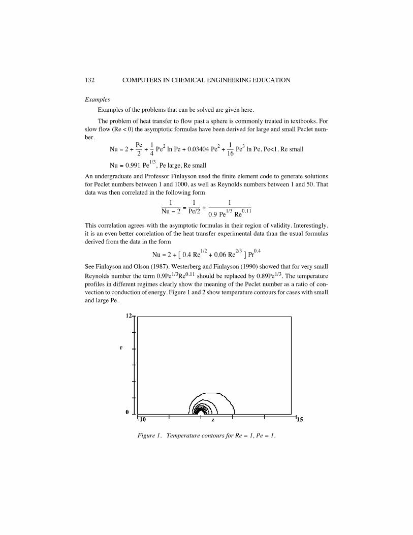
Examples
Examples of the problems that can be solved are given here.
The problem of heat transfer to flow past a sphere is commonly treated in textbooks. Forslow flow (Re < 0) the asymptotic formulas have been derived for large and small Peclet num-ber.
An undergraduate and Professor Finlayson used the finite element code to generate solutionsfor Peclet numbers between 1 and 1000, as well as Reynolds numbers between 1 and 50. Thatdata was then correlated in the following form
This correlation agrees with the asymptotic formulas in their region of validity. Interestingly,it is an even better correlation of the heat transfer experimental data than the usual formulasderived from the data in the form
See Finlayson and Olson (1987). Westerberg and Finlayson (1990) showed that for very small
Reynolds number the term 0.9Pe
1/3
Re
0.11
should be replaced by 0.89Pe
1/3
. The temperatureprofiles in different regimes clearly show the meaning of the Peclet number as a ratio of con-vection to conduction of energy. Figure 1 and 2 show temperature contours for cases with smalland large Pe.
Figure 1. Temperature contours for Re = 1, Pe = 1.
Nu = 2 + Pe2
+ 14
Pe2 ln Pe + 0.03404 Pe2 + 116
Pe3 ln Pe, Pe<1, Re small
Nu = 0.991 Pe1/3
, Pe large, Re small
1Nu − 2 =
1Pe/2 +
1
0.9 Pe1/3
Re0.11
Nu = 2 + [ 0.4 Re1/2
+ 0.06 Re2/3
] Pr0.4

Transport Phenomena 133
Figure 2. Temperature contours for Re=1, Pe=20.
Another example is the study of concentration distribution of adenosine diphosphatewhich is released from a platelet membrane during thrombus growth (Folie and McIntire1989). The goal was to model thrombi of various shapes and dimensions. Because the finiteelement method can easily model changes in shape it is possible to study the effect of geometry.
Another example of a problem involving complicated geometry is the design of a thermalconductivity cell, as shown in Fig. 3. Calculations can determine the errors caused by conduc-tion through the plexiglass and the heat losses to the sourrounds. One dimensional calculationsshould be done first to give an estimate, and the estimate can be checked with the more detailedcalculations.
Figure 3. Thermal conductivity cell.

134 COMPUTERS IN CHEMICAL ENGINEERING EDUCATION
The last example is a problem to design a slotted-electrode electrochemical cell, as de-scribed by Orazem and Newman (1984). The problem can be reduced to that shown in Fig. 4,which is easily solved using the code for heat conduction. The student can then consider otherdesigns (geometries) to insure that the current is uniform along the face.
Slotted-electrode electrochemical cell
Figure 4. Problem description for slotted-electrode electro-chemical cell.
Computational Fluid Dynamics
A
t the advanced undergraduate and graduate levels, the equations needed for the study oftransport phenomena become more difficult. Two-dimensional transient, three spatial dimen-sions, nonlinear physical properties and convective model components are a few of the com-
semiconductor
glass
counterelectrode
νhνh νh
F
E
B
A
ϕ=1
ϕ=0
ϕ = 0n
on all other surfaces
∇ ϕ = 0 in the domain2
t h
L
G
L / h = 2.5 t / G = 0.25
h / G = 1

Transport Phenomena 135
plications that arise with more realistic problem specifications. The first method of attack is tosimplify the problem so that perturbation methods, Green’s functions or transforms can be used(Finlayson, 1980; Denn, 1980; Leal, 1992).
In general, numerical methods will be needed to solve problems with complicated geom-etry or nonlinear effects. Computational fluid dynamics (CFD) is the name commonly appliedto the study of fluid flows using computer simulation methods. Other transport processes, suchas heat and mass transfer, are also included in CFD since many problems involve the solutionof coupled transport processes. The use of numerical methods to solve transport process prob-lems, with either coupled or uncoupled phenomena, has a long history that precedes the use ofcomputers. The current availability of powerful computers and the development of sophisticat-ed discretization algorithms for the solution of the partial differential equation (PDE) setsfound in transport problems has led to the wide use of CFD in industry and academe.
The conservation equations for mass, momentum and energy require constitutive relationsto form a closed set of equations. In general, the exact solution cannot be found and we seek anapproximate solution to the state variables which will be defined at discrete points, or nodes,within the domain. There may be local approximating polynomials which interpolate the statevariables between sets of neighboring nodes. The discretization method replaces the PDE setby an algebraic or differential equation set. For steady state problems, the PDE would be con-verted to a set of algebraic equations, the discrete equation set, with an equation for each statevariable at each node. In transient problems, algorithms exist to generate algebraic equationsfor each state variable at each node for a given point in time. The method of lines, as appliedto transient PDE sets, generates a set of differential equations which define the value of eachstate variable at each node as a function of time.
We can write a general steady state differential equation for the state variables as follows,which applies to the conserved species:
Given an approximation to
φ
called
θ
, which is inserted into the governing PDE,
The magnitude of R, the residual error, varies locally and measures how well the conser-vation equation is being satisfied at a particular point in space. The Method of Weighted Re-siduals (MWR) defines a set of algebraic relationships between the values
θ
i
(which are theapproximated values of the state variables at each node) and its neighboring nodal values. Theweighted integral of R is forced to zero through
The choice of W, the weighting function, determines the type of method. The numericalschemes that are most often used include: finite differences, finite volumes, finite elements andcollocation methods. The
finite difference
method has a value of W=1 at node i, zero elsewhere,and thus the residual is forced to zero at each node. The derivatives of the state variables areapproximated using Taylor Series expansions. If the approximation to
θ
is given by a polyno-
∇• ( u + (- )) - S = 0ρ φ φΓ∇ (1)
∇• ( u +(- )) - S = Rρ θ θΓ∇ (2)
V
WRdV = 0∫ (3)

136 COMPUTERS IN CHEMICAL ENGINEERING EDUCATION
mial and the weighting function is W=1 at specified sampling points, the method is called
col-location
(Finlayson, 1980).
Finite element
methods use a definition of a polynomial for
θ
overa small region within the domain with the values of the state variables at defined nodes suchthat
The terms N
i
are known as shape functions and are defined within each element such thattheir value is 1 at the node i, a value between 0 and 1 within the element and zero outside theelement. The choice of W defines the particular type of finite element method. For example,W= N
i
defines the widely used Galerkin finite element method.
Finally,
finite or control volume
methods can be derived by starting with W=1 within acontrol volume around the node i and zero outside of this subdomain (Patankar, 1980). The in-tegral can then be broken into a volume integral and a surface integral which satisfies the inte-gral form of the conservation equations
Variations on the finite volume methods depend on how the control volume is chosenaround the nodal points and the manner in which gradient terms are approximated using neigh-boring nodes and their respective control volumes. Thus, from a basic definition, one can de-rive the basic versions of all the popular methods used in solving advanced CFD problems. Themethods share the common feature of gridding where the network of nodes, which will definethe points at which the state variables will be determined, is chosen and some methods requirethe definitions for the elements or subdomains. The basic steps for all the methods are the same:choose the conservation equations and terms within the equations appropriate to the problem,divide the domain into an appropriate set of nodes and subdomains/elements, assemble the dis-cretized forms of the PDEs as (non)linear algebraic equations and solve the equation set.
Graduate courses which use the concepts described above vary widely in content depend-ing on the objectives for the student. One approach is to do an overview of the different dis-cretization methods and then provide a series of problems which require a numerical analysis.Commercial CFD simulators are widely used both in industry and academe, for example: FLU-ENT/BFC which uses the finite volume method (Fluent Inc., 1990), FIDAP which uses the fi-nite element method (FDI, 1993) and NEKTON which uses the spectral element method(Fluent Inc., 1992). Readers are referred to the annual Software Directory published by
Chem-ical Engineering Progress
for current listings of available software applicable to chemical en-gineering problems and the article by Wolfe (1991). Commercial simulators have a variety oftutorial problems based on practical problems taken from the literature. It is common to askstudents to modify existing meshes or modify boundary conditions to simulate another prob-
θ θ(x,y z) = N x y zi
(e)
i i(e), ( , , )∑ (4)
∀
∫ ∑ ∑∇•
(e)
ii
(e)
i(e)
ii
(e)
i(e)
iN u N ) + (- ( N ))) - S dV = 0( (ρ θ θΓ∇ (5)
(6)i iA V
( u + (- )) ndA - SdV = 0∫ ∫•ρ θ θΓ∆
Transport Phenomena 137
lem. It is important to recognize the amount of time it takes to generate a good mesh for thesolution of realistic problems. The general rule-of-thumb is that 80% of the user’s time will bein the development of the mesh. In posing problems for students it is important to keep the timerequirements in mind when dealing with complicated geometry when an existing mesh is notavailable to the student. The problems that are currently available in commercial CFD packagelibraries span a wide spectrum of applications and include: crystal growth, polymer flows, po-rous media flows, electronic packaging cooling and particle-laden fluid flows. All the packageshave an interface to develop the mesh and post-processing capabilities to visualize the resultingflow velocities and other state variables in the domain. Though implementations exist for thepersonal computer platform (PC-DOS and Macintosh), most realistic problems require a work-station.
It is very important to build up the expertise of the student by encouraging the solution ofproblems for which experimental data are available. The amount of data produced by a CFDcode can be overwhelming, particularly in 3-D problems, and so a thorough grounding in theexpected flows and fluxes of well-characterized problems provides a good basis for analysis ofmore complicated problems. The effects on the calculated state variable values of mesh densi-ty, coupling of transport processes and sensitivity of the solution to physical property parame-ters requires skills gained through experience. It is too easy to determine a steady-state solutionto a problem for which no steady-state exists!
Another approach for teaching CFD courses is to develop a particular method in the class-room and have the students implement subroutines as they learn the important concepts of themethod. For example, students may implement a basic meshing algorithm, the formulation ofthe discretized equations and the linear equation solver. Visualization software should be usedto simplify analysis of the results. This type of course gives the student a better perspective onthe development of the equations and the problems in solving the final set of equations, but lim-its their exposure to more complicated problem formulations. Sample reference textbooks foreach of the methods as applied to CFD include: Anderson et al. (1984) for finite differences,Baker (1983) and Dhatt and Touzot (1984) for finite elements and Patankar (1980) for controlvolumes. Minkowycz et al. (1988) and Fletcher (1988) provide chapters dedicated to the use ofdifferent numerical schemes common in CFD applications.
In summary, CFD and the numerical solution of the transport equations are importantfields which are widely taught at the graduate level and are beginning to be exposed in the un-dergraduate curriculum. The wider use of CFD has been accelerated by the combined availabil-ity of faster computers, more sophisticated numerical solution techniques and graphic tools tovisualize the results.
References
Anderson, D.A., J.C. Tannehill and R.H. Pletcher (1984).
Computational Fluid Mechanics and Heat Transfer,
Hemisphere, New York.
Baker, A.J. (1983).
Finite Element Computational Fluid Mechanics,
Hemisphere, New York.
Bird, R.B., W.E. Stewart, E.N. Lightfoot (1960).
Transport Phenomena
, Wiley, New York.
Denn, M.M. (1980).
Process Fluid Mechanics
, Prentice-Hall, New York.

138 COMPUTERS IN CHEMICAL ENGINEERING EDUCATION
Dhatt, G., and G. Touzot (1984).
The Finite Element Method Displayed
, John Wiley & Sons, New York.
Fahien, R. (1983).
Fundamentals of Transport Phenomena
, McGraw-Hill, New York.
Finlayson, B.A. (1980).
Nonlinear Analysis in Chemical Engineering
, McGraw-Hill, New York.
Finlayson, B.A. and J.W. Olson (1987). Heat Transfer to Spheres at Low to Intermediate Reynolds Numbers.
Chemical Engineering Communications
,
58
, 431-447.
Fletcher, C.A.J. (1988).
Computational Techniques for Fluid Dynamics, Volumes 1 and 2
, Springer-Verlag, NewYork.
Fluent Inc. (1980).
FLUENT and FLUENT/BFC 4.0 Manual
, Lebanon, New Hampshire.
Fluent Inc. (1992).
NEKTON 2.85 Manual
, Lebanon, New Hampshire.
Fluid Dynamics International, Inc. (1993).
FIDAP 7.0 Manuals
, Evanston, Illinois.
Folie, B.J. and L.V. McIntire (1989). Mathematical Analysis of Mural Thrombogenesis.
Biophys. J
.,
56
, 1121-1141.
Leal, L.G. (1992).
Laminar Flow and Convective Transport Processes: Scaling Principles and Asymptotic Anal-ysis
, Butterworth-Heinemann, Boston.
Minkowycz, W.J. et al. (1988).
Handbook of Numerical Heat Transfer
, John Wiley & Sons, Inc., New York.
Orazem, M. and J. Newman (1984). Primary Current Distribution and Resistance of a Slotted-Electrode Cell.
J.Electrochem. Soc
.,
131
, 2857-2861.
Patankar, S.V. (1980).
Numerical Heat Transfer and Fluid Flow
, Hemisphere, New York.
Westerberg, K.W. and B.A. Finlayson (1990). Heat Transfer to Spheres from a Polymer Melt,
Numerical HeatTransfer, Part A
,
17
, 329-348.
Wolfe, A. (1991). CFD Software: Pushing Analysis to the Limit,
Mechanical Engineering
, January, 48-54.

139
SEPARATIONS PROCESSES
Ross TaylorClarkson UniversityPotsdam, NY 13699
Abstract
The equilibrium stage has been used for modeling separations process problems fornearly 100 years. The model equations are particularly amenable to computer solution,and teachers of separations courses were among the first to introduce computers intoundergraduate chemical engineering curricula. CACHE has supported developmentand use of interactive instructional modules for the separations area, and has promoteddistribution of the powerful
ChemSep
multicomponent distillation design tool for usein separations courses.
In recent years, it has become possible to model separations processes using mass-transfer, rate-based
nonequilibrium
models. These nonequilibrium models are likely tosee increased use in the future, particularly for simulating nonideal systems, systemswith reaction, and/or processes with multiple feeds and products. This trend toward in-troduction of nonequilibrium (and also dynamic) models should act as a spur for closerintegration of separations and mass-transport courses.
Introduction
A recent advertisement for a journal claims that there are 40,000 distillation columns andthat operating these columns requires 7% of all of the energy consumed in the United Statesalone. When we consider all of the distillation columns elsewhere in the world, as well as allthe closely related operations of absorption, stripping and extraction, it is clear that, even ifthese figures are significantly in error (other published figures put the energy consumption atabout 3%), the classical separation processes are unusually important unit operations.
Chemical engineers (whether they are professionals in industry or university students)have been solving separation process problems using the
equilibrium stage model
for about 100years (since Sorel first used the model for the distillation of alcohol). The key assumption inthe equilibrium stage model is that the vapor and liquid streams leaving a stage are in equilib-rium with each other. The equations that model equilibrium stages are known as the
MESH
equations. The
M
equations are the Material balance equations, the
E
equations are the equilib-rium relations, the
S
equations are the mole fraction summation equations, and the
H
equationsare the enthalpy balance equations. The unknown variables determined by solving these equa-tions are the mole fractions of both phases, the stage temperatures, and the flow rate of eachphase.

140 COMPUTERS IN CHEMICAL ENGINEERING EDUCATION
There can be few other mathematical models in any branch of engineering which are sowell suited to computer solution and that have prompted the development of so many truly dif-ferent algorithms as have the
MESH
equations of the equilibrium stage model. Indeed, it wouldnot be too far from the truth to claim that it is equilibrium stage calculations that brought com-puting into chemical engineering (or should that be chemical engineers to computers?). Sincecomputers became available in the late 1950s hardly a year has passed without the publicationof at least one new algorithm for solving the equilibrium stage model equations and, in manyyears, several new algorithms have appeared. Most of the better numerical methods (and someof the not so good ones) have been used in the solution of equilibrium stage problems. Indeed,a good test of a numerical method might therefore be to see if it can be used to solve distillationproblems.
It is not our intention to provide a complete review of computer-based methods for sepa-ration process calculations; readers can consult one of several textbooks that includes some dis-cussion on computer-based methods (Smith, 1964; King, 1980; Henley and Seader, 1981).Other books have focused almost entirely on the computational aspects (Holland, 1963, 1975,1981) and Seader (1985) gives an interesting history of equilibrium stage separations calcula-tion methods with more detail than is appropriate this brief article.
CACHE Contributions
Nowadays, even chemical engineering students solve their distillation problems usingcomputer software. In this section we review the part that CACHE has played in making thispossible.
While not a CACHE product, it would be remiss of us not to mention the collection ofprograms for separation process simulation by Hanson, Duffin, and Somerville (1962). Theirbook included several programs in Fortran for solving a wide variety of multistage separationprocess problems including distillation, absorption, stripping and liquid-liquid extraction. Achapter at the end of the book discusses the peculiar difficulties associated with interlinked col-umns. Several introductory chapters serve to introduce the reader to “a sufficient number oftechniques... to make possible convergent solutions to
any
problem” (emphasis added). The op-timism expressed in the above quotation is interesting for, despite many developments thathave taken place over the past 30 years, we still have not reached that happy (for some) situa-tion where all of our equilibrium stage separation process problems can be solved the first timethey are attempted. We are, however, a great deal closer to that goal.
Included in the CACHE series
Computer Programs for Chemical Engineering Education
published in 1972 (and mentioned elsewhere in this volume as well) was a volume entitled
Stagewise Computations
(Christensen, 1972). The paperback edition included descriptions, ex-amples of usage, and listings of 17 Fortran programs for modeling such operations as counter-current leaching, liquid-liquid extraction, batch distillation, and multicomponent distillation,stripping and absorption. The programs in this book represented a cross-section of computer-ized implementations of old-fashioned calculation methods, originally devised for solving sep-arations process problems by hand, and programs that implemented methods that betterrepresented the state of the art as it was at the time. These programs were used at many univer-sities around the world.

Separations Processes 141
Among the programs in the CACHE collection are two by N.S. Berman and O.C. Sandallthat implement the stage-to-stage calculation method developed by Lewis and Matheson(1932) (and refined by others). D.M. Watt provided a program that used another algorithmfrom the same era, the method of Thiele and Geddes (1933). L.L. Hovey provided an imple-mentation of the Amundsen - Pontinen (1957) method. This was one of the first methods to ex-ploit matrix algebra in the solution of counter-current separations problems.
WHENDI
by P.J. Johansen and J.D. Seader implements the Wang and Henke (1966) bub-ble point method for distillation, which is a modification of the Amundsen - Pontinen (1957)method.
STAB
, by the same authors plus T. Shinohara, solves absorption and stripping prob-lems using the sum-rates method (Sujata, 1961; Burningham and Otto, 1967). Bubble point andsum-rates methods belong to a class of algorithm known as equation-tearing methods and havebeen used in industry for several decades. These methods pair model equations and variablesin two loops and alternately solve the equations in each loop until convergence is reached. Bub-ble point methods use temperatures as inner loop variables and the total vapor flow profile isadjusted in an outer loop by solving the energy balances. Sum-rates methods fix the tempera-ture and pressure profile for the column and the mass balance and phase equilibrium equationsare solved simultaneously for the component flow rates in an inner loop. The energy balanceequations are solved in an outer loop in order to adjust the temperature profile.
J.W. Tierney contributed a program that could handle interlinked columns. The programemployed an algorithm that falls into the class of 2N Newton methods that Tierney and his co-workers helped to develop in the late 1960s and early 1970s (Tierney and Bruno, 1967; Tierneyand Yanosik, 1969). In these methods the temperatures and flows are adjusted simultaneouslyusing Newton’s method.
Newton’s method now is widely used in commercial simulation programs (although it hastaken many years longer than it should to have gained the measure of acceptance it now en-joys). To the best of our knowledge, a method to solve
all
the MESH equations for all stagesat once using Newton’s method was first described by Whitehouse (1964). Among otherthings, Whitehouse’s code could solve problems involving purity specifications or of
T, V, L
or
Q
on any stage. Interlinked systems of columns and nonideal solutions also could be han-dled. Unfortunately, Whitehouse’s work was published in a rather obscure proceedings volume(Stainthorp and Whitehouse, 1967) and had essentially no influence on the development ofcomputer-based simulation methods. The credit for showing us how to use Newton’s methodfor separation process calculations, therefore, goes to Naphtali and Sandholm, (1971) and toGoldstein and Stanfield (1970) for distillation and to E.C. Roche (1971), who applied the meth-od to liquid-liquid extraction and who contributed the program
LIQLIQ
that is included in theCACHE collection.
In 1987 CACHE distributed to supporting departments a collection of computer-basedlessons containing “open-ended” design type problems for use in courses other than the cap-stone design course (Seider, 1987). Among the six lessons were three for separations courses:Supercritical fluid extraction (by J. Kellow, M.L. Cygnarowicz, and W.D. Seider, Pennsylva-nia), Gas Absorption with Chemical Reaction (by K. Nordstrom and J.H. Seinfeld, Cal Tech),and Design of Flash Vessels and Distillation Towers (by B.A. Finlayson, E.W. Kaler, and W.J.Heideger, Washington) based on short-cut methods of column design. The major change in

142 COMPUTERS IN CHEMICAL ENGINEERING EDUCATION
computing practices brought about by the personal computer in the decade of the 1980s is ev-ident in this release; the material was provided on floppy disks for use with IBM PC compatiblecomputers.
In 1992 CACHE made available
ChemSep
, a computer software system developed by R.Taylor and H.A. Kooijman (1992). As a piece of software
ChemSep
is much more closely re-lated to flowsheet simulation programs than to the computer-based lessons and modules dis-cussed above. The program was created for use in university separations courses (but may alsobe useful in thermodynamics and design) but also can be (and is) used by professionals in in-dustry.
ChemSep
features a menu-driven user interface and simulation programs that can han-dle flash, and single distillation, absorption and liquid-liquid extraction columns with multiplefeeds and sidestreams. Many of the most widely used thermodynamic models are available in
ChemSep
and Newton’s method is used to solve the large, sparse system of nonlinear equa-tions. The CACHE version of the package includes a database for 189 different chemicals andcan handle up to 10 components and 100 stages.
H.S. Fogler and S. M. Montgomery (1993) have created a collection of interactive (per-sonal) computer modules for chemical engineering instruction. There are five of these modulesfor separations courses including: BASIS - An introduction to Separation Processes, CAS-CADES - Liquid-liquid Extraction, MCCABE - Binary Distillation (via the McCabe-Thielemethod), ABSORP - Packed absorber design, and MEMBRANES - Spiral membrane processoptimization. These modules feature animations within a graphical user interface that allowstudents to interactively review material and to carry out simulated experiments (see Figs. 1and 2).
Figure 1. Screen image from CACHE module ABSORP for absorption column design.

Separations Processes 143
Figure 2. Screen image from CACHE module MCCABE for binary distillation.
It is interesting to contrast the first CACHE programs with their more recent offerings.
WHENDI
, for example, is just 635 lines of Fortran. Contrast this with
ChemSep
which consistsof about 100,000 lines of Fortran (of which about 10,000 is just the part that computes physicalproperties) and Turbo Pascal. The comparison is, of course, not entirely fair since
WHENDI
wasnever intended to be able to handle the range of problems that can be tackled with
ChemSep
.Nevertheless, it serves to illustrate one of the negative aspects of modern software, a trend toever larger software systems; a trend that, fortunately, is countered by the ever increasing speedand capacity of computer hardware.
The Impact of Computer-Based Tools on Separations Courses
Perhaps nowhere else in the chemical engineering curriculum has the impact of computersbeen greater than in the teaching of separations. The availability of computer-based tools suchas
ChemSep
make it possible to include realistic multicomponent distillation design problemsin the first undergraduate course on separations. In spite of these developments, the graphicalMcCabe-Thiele method, devised in the 1920s, combines simplicity and elegance and remainsa useful method for the analysis of distillation type operations, even for multicomponent sys-tems, as shown in Fig. 3. Indeed, graphical techniques (McCabe-Thiele diagrams and columnprofiles such as those in Figs. 4 and 5) for the visualization of numerical simulation results areextremely valuable instructional tools. (With the exception of Figs. 1 and 2, all of the illustra-tions in this article were created by
ChemSep
, printed to a file using one of several graphic im-age formats supported by the program, and imported into the word processor used to create thisarticle.)
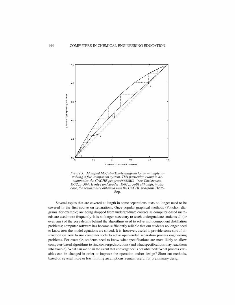
144 COMPUTERS IN CHEMICAL ENGINEERING EDUCATION
Figure 3. Modified McCabe-Thiele diagram for an example in-volving a five component system. This particular example ac-companies the CACHE program
WHENDI
(see Christensen, 1972, p. 384; Henley and Seader, 1981, p 568) although, in this case, the results were obtained with the CACHE program
Chem-Sep
.
Several topics that are covered at length in some separations texts no longer need to becovered in the first course on separations. Once-popular graphical methods (Ponchon dia-grams, for example) are being dropped from undergraduate courses as computer-based meth-ods are used more frequently. It is no longer necessary to teach undergraduate students all (oreven any) of the gory details behind the algorithms used to solve multicomponent distillationproblems; computer software has become sufficiently reliable that our students no longer needto know
how
the model equations are solved. It is, however, useful to provide some sort of in-struction on how to use computer tools to solve open-ended separation process engineeringproblems. For example, students need to know what specifications are most likely to allowcomputer-based algorithms to find converged solutions (and what specifications may lead theminto trouble). What can we do in the event that convergence is not obtained? What process vari-ables can be changed in order to improve the operation and/or design? Short-cut methods,based on several more or less limiting assumptions, remain useful for preliminary design.
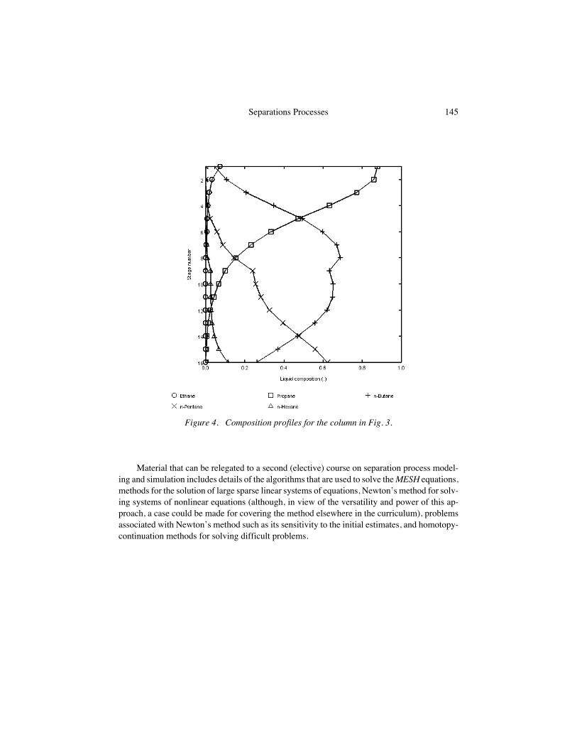
Separations Processes 145
Figure 4. Composition profiles for the column in Fig. 3.
Material that can be relegated to a second (elective) course on separation process model-ing and simulation includes details of the algorithms that are used to solve the
MESH
equations,methods for the solution of large sparse linear systems of equations, Newton’s method for solv-ing systems of nonlinear equations (although, in view of the versatility and power of this ap-proach, a case could be made for covering the method elsewhere in the curriculum), problemsassociated with Newton’s method such as its sensitivity to the initial estimates, and homotopy-continuation methods for solving difficult problems.
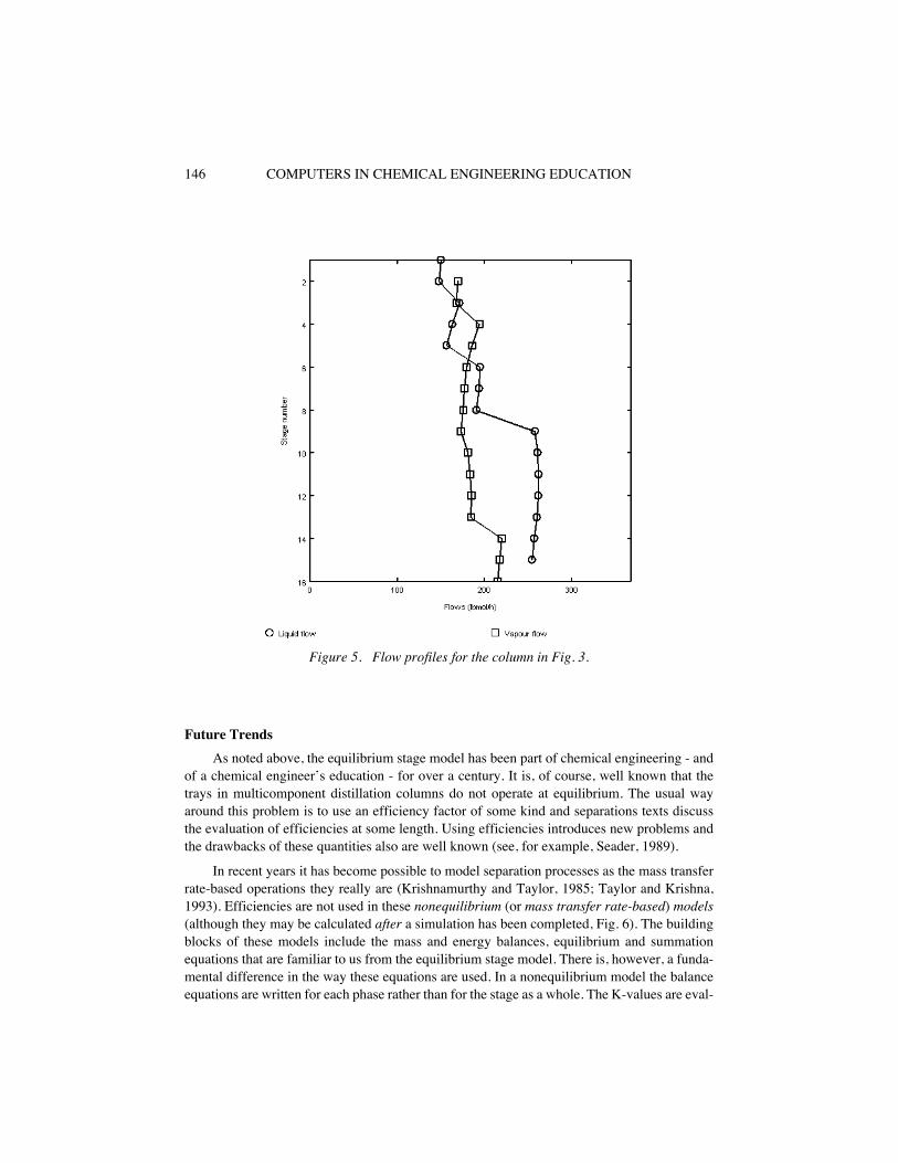
146 COMPUTERS IN CHEMICAL ENGINEERING EDUCATION
Figure 5. Flow profiles for the column in Fig. 3.
Future Trends
As noted above, the equilibrium stage model has been part of chemical engineering - andof a chemical engineer’s education - for over a century. It is, of course, well known that thetrays in multicomponent distillation columns do not operate at equilibrium. The usual wayaround this problem is to use an efficiency factor of some kind and separations texts discussthe evaluation of efficiencies at some length. Using efficiencies introduces new problems andthe drawbacks of these quantities also are well known (see, for example, Seader, 1989).
In recent years it has become possible to model separation processes as the mass transferrate-based operations they really are (Krishnamurthy and Taylor, 1985; Taylor and Krishna,1993). Efficiencies are not used in these
nonequilibrium
(or
mass transfer rate-based
)
models
(although they may be calculated
after
a simulation has been completed, Fig. 6). The buildingblocks of these models include the mass and energy balances, equilibrium and summationequations that are familiar to us from the equilibrium stage model. There is, however, a funda-mental difference in the way these equations are used. In a nonequilibrium model the balanceequations are written for each phase rather than for the stage as a whole. The K-values are eval-

Separations Processes 147
uated at the temperature, pressure, and composition of the interface, which is assumed to be anequilibrium surface, offering no resistance to mass transfer. Equations that model the mass andenergy transfer across the phase boundary are included in the model and solved simultaneouslywith the other equations. Mass and energy are transferred across the interface at rates that de-pend on the extent to which the phases are
not
in equilibrium with each other. These rates arecalculated from models of mass transfer in multicomponent systems (see Taylor and Krishna(1993) for an extended discussion of such models). Mass and heat transfer coefficients and in-terfacial areas must be computed from empirical correlations or theoretical models. These co-efficients depend on the column design as well as on its method of operation. Nonequilibriummodels can be used to simulate packed columns just as easily as they can tray columns, therebyavoiding the use of HETPs (Height Equivalent to a Theoretical Plate). A nonequilibrium col-umn model was included in Version 3 of the CACHE product ChemSep.
It is very likely that nonequilibrium models will see increased use in the future; they willbe particularly useful for simulating nonideal systems, systems with chemical reaction, andlow-efficiency systems (this includes some nonideal separations and many gas absorption pro-cesses), and columns with multiple feeds and products. A thorough understanding of masstransfer (with or without simultaneous chemical reaction) in multicomponent systems will beessential for the engineer (and student) working with nonequilibrium models. It is pertinent topoint out that mass transfer in binary systems constitutes a very special case in that none of theinteresting phenomena that can take place in systems with more than two components can oc-cur. Multicomponent mass transfer effects can manifest themselves in interesting ways, includ-ing causing distillation point efficiencies of different components to
not
be equal fromcomponent to component or from tray to tray (as they are so often assumed to be) as is clearlyevident in Fig. 6 and, to a lesser degree, Fig. 7. Any emphasis on mass transfer rate based mod-els in the future should act as a spur to educators to more tightly integrate courses on separa-tions and mass transport; the latter will need to be modified in order to cover the elements ofmulticomponent mass transfer (see Taylor and Krishna, 1993).
The equations that describe multicomponent mass transport (the Maxwell-Stefan equa-tions) have, in fact, been with us even longer than has the equilibrium stage model althoughtheir application to modeling stagewise separations is a relatively recent development. Howev-er, not only do the Maxwell-Stefan equations allow us to model mass transfer in conventionaloperations such as distillation, absorption, and liquid-liquid extraction, they also describe masstransfer in all of the less common separation operations such as membrane processes, the ultra-centrifuge, thermal diffusion columns, and many more. Indeed, the Maxwell-Stefan formula-tion of mass transfer can provide a basis for unifying the treatment of separation processes(Krishna, 1987).
Models of the dynamic behavior of column performance are being used more frequentlyin industry. Improvements in hardware and software will mean that ten years from now therewill be no excuse for not using a dynamic model to explore the operation of a real distillationcolumn. Dynamic models will become available that are based on fundamental mass and ener-gy transfer processes. These models will also be used in undergraduate courses and will makeit possible to provide more convincing software demonstrations of how real columns behave.

148 COMPUTERS IN CHEMICAL ENGINEERING EDUCATION
Figure 6. Efficiency profiles calculated following a nonequilib-rium simulation of the column in Figs. 3 to 5. The usual assump-
tion of equal component efficiencies is clearly inappropriate.
Of course, models based on equilibrium stage concepts will not be abandoned, nor is thereany need to do so. New approaches to process visualization (see Fig. 8), and design and anal-ysis of separation processes using equilibrium stage models have been pioneered by M.F.Doherty, M.F. Malone and their coworkers at the University of Massachusetts (see, for exam-ple, Fidkowski
et al
., 1991; Doherty and Buzad, 1992; Julka and Doherty, 1993). At the timeof writing, however, there is no software product that implements their methods that is avail-able from CACHE.

Separations Processes 149
Figure 7. Modified McCabe-Thiele diagram provides an inter-esting view of the effects of mass transfer in stagewise separa-
tions. Note how the triangles representing the trays do not reach the equilibrium line, demonstrating that they are not equilibrium
stages.
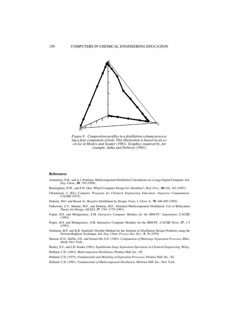
150 COMPUTERS IN CHEMICAL ENGINEERING EDUCATION
Figure 8. Composition profiles in a distillation column process-ing a four component system. This illustration is based on an ex-ercise in Henley and Seader (1981). Graphics inspired by, for
example, Julka and Doherty (1993).
References
Amundsen, N.R., and A.J. Pontinen, Multicomponent Distillation Calculations on a Large Digital Computer,
Ind.Eng. Chem
.,
50
, 730 (1958).
Burningham, D.W., and F.D. Otto, Which Computer Design for Absorbers?,
Hyd. Proc.
,
40
(10), 163 (1967).
Christensen, J. (Ed.)
Computer Programs for Chemical Engineering Education: Stagewise Computations
,CACHE (1972).
Doherty, M.F. and Buzad, G., Reactive Distillation by Design,
Trans. I. Chem. E
.,
70
, 448-458 (1992).
Fidkowski, Z.T., Malone, M.F., and Doherty, M.F., Nonideal Multicomponent Distillation: Use of BifurcationTheory for Design,
AIChEJ
,
37
, 1761-1779 (1991).
Fogler, H.S. and Montgomery, S.M.
Interactive Computer Modules for the IBM-PC: Separations
, CACHE(1993).
Fogler, H.S. and Montgomery, S.M. Interactive Computer Modules for the IBM-PC, CACHE News,
37
, 1-5(1993).
Goldstein, R.P. and R.B. Stanfield, Flexible Method for the Solution of Distillation Design Problems using theNewton-Raphson Technique,
Ind. Eng. Chem. Process Des. Dev.
,
9
, 78 (1970)
Hanson, D.N., Duffin, J.H., and Somerville, G.F. (1962).
Computation of Multistage Separation Processes
, Rhei-nhold, New York.
Henley, E.J., and J.D. Seader (1981).
Equilibrium-Stage Separation Operations in Chemical Engineering
, Wiley.
Holland, C.D. (1963).
Multicomponent Distillation
, Prentice Hall, Inc., NJ.
Holland, C.D. (1975).
Fundamentals and Modeling of Separation Processes
, Prentice Hall, Inc., NJ.
Holland, C.D. (1981).
Fundamentals of Multicomponent Distillation
, McGraw-Hill, Inc.; New York.
Separations Processes 151
Julka, V. and Doherty, M.F. (1993). Geometric Nonlinear Analysis of Multicomponent Nonideal Distillation: ASimple Computer-Aided Design Procedure,
Chem. Eng. Sci.
,
48
, 1367-1391.
Kooijman, H.A. and Taylor, R. (1992).
ChemSep
- Another Software System for the Simulation of Separation Pro-cesses,
CACHE News
,
35
, 1-9.
Krishna, R. (1987). A Unified Theory of Separation Processes Based on Irreversible Thermodynamics,
Chem.Eng. Commun.
,
59
, 33-64.
Krishnamurthy, R. and Taylor, R. (1985). A Nonequilibrium Stage Model of Multicomponent Separation Process-es. I - Model Development and Method of Solution,
A.I.Ch.E.J.
,
31
(3), 449-456.
Lewis, W.K. and G.L. Matheson (1932). Studies in Distillation: Design of Rectifying Columns for Natural AndRefinery Gasoline,
Ind. Eng. Chem.
,
24
(5), 496.
Naphtali, L.M. and D.P. Sandholm (1971). Multicomponent Separation Calculations by Linearization,
AIChE
J.,
17
(1), 148.
Roche, E.C. (1971). General Design Algorithm for Multistage Counter Current Equilibrium Processes,
Brit.Chem. Eng.
16
, 821.
Seader, J.D. (1985). The BC (Before Computers) and AD of Equilibrium Stage Operations,
Chem. Eng. Ed
.,Spring, 88.
Seader, J.D. (1989). The Rate-Based Approach to Modeling Staged Separations,
Chem. Eng. Progress
, 41-49, Oc-tober.
Seider, W.D. (1987).
CACHE IBM PC Lessons for Chemical Engineering Courses Other Than Design and Con-trol
, CACHE.
Stainthorp, F.P., and Whitehouse, P.A. (1967). General Computer Programs for Multistage Counter Current Sep-aration Problems - I: Formulation of the Problem and Method of Solution,
I. Chem. E. Symposium Series
,
23
, 181.
Smith. B.D. (1964).
Design of Equilibrium Stage Processes
, McGraw-Hill, New York.
Sujata, A.D. (1961). Absorber-Stripper Calculations Made Easier.
Hyd. Proc.
, 40 (12), 137.
Taylor, R. and Krishna, R. (1993).
Multicomponent Mass Transfer
, Wiley, New York.
Thiele, E.W., and R.L. Geddes (1933). Computation of Distillation Apparatus for Hydrocarbon Mixtures,
Ind.Eng. Chem.
,
25
, 289.
Tierney, J.W. and J.A. Bruno (1967). Equilibrium Stage Calculations, AIChE J.,
13
(3), 556.
Tierney, J.W., and J.L. Yanosik (1969). Simultaneous Flow and Temperature Correction in the Equilibrium StageProblem,
AIChE J.
,
15
(6), 897.
Wankat, P.C. (1988).
Equilibrium Staged Separations
, Elsevier, New York.
Wang, J.C. and G.E. Henke (1966). Tridiagonal Matrix for Distillation,
Hyd. Proc.
,
45
(8), 155.
Whitehouse, P.A. (1964). PhD Thesis in Chemical Engineering, University of Manchester Institute of Science andTechnology, April.