Cache-Adaptive Exploration: Experimental Results and Scan...

Cache-Adaptive Exploration:Experimental Results and Scan-Hiding for Adaptivity

Andrea Lincoln

Computer Science and Artificial Intelligence Laboratory

Massachusetts Institute of Technology

[email protected]

Quanquan C. Liu



[email protected]

Jayson Lynch



[email protected]

Helen Xu



[email protected]

ABSTRACT

Systems that require programs to share the cache such as shared-

memory systems, multicore architectures, and time-sharing systems

are ubiquitous in modern computing. Moreover, practitioners have

observed that the cache behavior of an algorithm is often critical

to its overall performance.

Despite the increasing popularity of systems where programs

share a cache, the theoretical behavior of most algorithms is not yet

well understood. There is a gap between our knowledge about how

algorithms perform in a static cache versus a dynamic cache where

the amount of memory available to a given program fluctuates.

Cache-adaptive analysis is a method of analyzing how well algo-

rithms use the cache in the face of changing memory size. Bender

et al. showed that optimal cache-adaptivity does not follow from

cache-optimality in a static cache. Specifically, they proved that

some cache-optimal algorithms in a static cache are suboptimal

when subject to certain memory profiles (patterns of memory fluc-

tuations). For example, the canonical cache-oblivious divide-and-

conquer formulation of Strassen’s algorithm for matrix multiplica-

tion is suboptimal in the cache-adaptive model because it does a

linear scan to add submatrices together.

In this paper, we introduce scan hiding, the first technique for

converting a class of non-cache-adaptive algorithms with linear

scans to optimally cache-adaptive variants. We work through a

concrete example of scan-hiding on Strassen’s algorithm, a sub-

cubic algorithm for matrix multiplication that involves linear scans

at each level of its recursive structure. All of the currently known

sub-cubic algorithms for matrix multiplication include linear scans,

however, so our technique applies to a large class of algorithms.

We experimentally compared two cubic algorithms for matrix

multiplication which are both cache-optimal when the memory

size stays the same, but diverge under cache-adaptive analysis.

Our findings suggest that memory fluctuations affect algorithms

Permission to make digital or hard copies of all or part of this work for personal or

classroom use is granted without fee provided that copies are not made or distributed

for profit or commercial advantage and that copies bear this notice and the full citation

on the first page. Copyrights for components of this work owned by others than the

author(s) must be honored. Abstracting with credit is permitted. To copy otherwise, or

republish, to post on servers or to redistribute to lists, requires prior specific permission

and/or a fee. Request permissions from [email protected].

SPAA ’18, July 16–18, 2018, Vienna, Austria© 2018 Copyright held by the owner/author(s). Publication rights licensed to ACM.

ACM ISBN 978-1-4503-5799-9/18/07. . . $15.00

https://doi.org/10.1145/3210377.3210382

with the same theoretical cache performance in a static cache dif-

ferently. For example, the optimally cache-adaptive naive matrix

multiplication algorithm achieved fewer relative faults than the

non-adaptive variant in the face of changing memory size. Our

experiments also suggest that the performance advantage of cache-

adaptive algorithms extends to more practical situations beyond

the carefully-crafted memory specifications in theoretical proofs of

worst-case behavior.

CCS CONCEPTS

•Theory of computation→Parallel computingmodels;Caching

and paging algorithms; •General and reference→ Experimen-tation;

KEYWORDS

cache adaptivity; scan hiding; adaptive constructions; external mem-

ory

ACM Reference Format:

Andrea Lincoln, Quanquan C. Liu, Jayson Lynch, and Helen Xu. 2018. Cache-

Adaptive Exploration: Experimental Results and Scan-Hiding for Adaptivity.

In SPAA ’18: 30th ACM Symposium on Parallelism in Algorithms and Architec-tures, July 16–18, 2018, Vienna, Austria. ACM, New York, NY, USA, 10 pages.

https://doi.org/10.1145/3210377.3210382

1 INTRODUCTION

Since multiple processors may compete for space in a shared cache

on modern machines, the amount of memory available to a single

process may vary dynamically. Programs running on multicore

architectures, shared-memory machines, and time-shared machines

often experience memory fluctuations. For example, Dice, Marathe

and Shavit [12] demonstrated that in practice, multiple threads

running the same programwill each get a different amount of access

to a shared cache.

Experimentalists have recognized the problem of changing mem-

ory size in large-scale scientific computing and have developed

heuristics [17–19] for allocation with empirical guarantees. Fur-

thermore, researchers have developed adaptive sorting and join

algorithms [10, 16, 20, 21, 27–29] that perform well empirically

in environments with memory fluctuations. While most of these

algorithms work well on average, they may still suffer from poor

worst-case performance [4, 5].

Session 5 SPAA’18, July 16-18, 2018, Vienna, Austria

213

https://doi.org/10.1145/3210377.3210382

https://doi.org/10.1145/3210377.3210382

In this paper, we continue the study of algorithmic design of

external-memory algorithms which perform well in spite of mem-

ory fluctuations. Barve and Vitter [4, 5] initiated the theoretical

analysis of such algorithms. Bender et al. [8] later formulated the

“cache-adaptive model” to formally study the effect of such memory

changes and analyzed specific “cache-adaptive” algorithms using

this model.Cache-adaptive algorithms are algorithms that use the

cache optimally in the face of memory fluctuations. They then intro-

duced techniques for analyzing some classes of divide-and-conquer

algorithms in the cache-adaptive model.

Cache Analysis Without Changing MemoryDespite the reality of dynamic memory fluctuations, the majority

of theoretical work on external-memory computation [25, 26] as-

sumes a fixed cache sizeM. The measure of interest in the external-

memory model is the number of I/Os, or fetches from external

memory, that an algorithm takes to finish its computation. Many

I/O-efficient algorithms in the fixed-memory model suffer from

poor performance whenM changes due to thrashing if the avail-

able memory drops.

Cache-oblivious algorithms [11, 13, 14] provide insight about

how to design optimal algorithms in the face of changing memory.

Notably, cache-oblivious algorithms are not parameterized by the

cache or cache line size. Instead, they leverage their recursive algo-

rithm structure to achieve cache-optimality under static memory

sizes. They are often more portable because they are not tuned

for a specific architecture. Although Bender et al. [7] showed that

not all cache-oblivious algorithms are cache-adaptive, many cache-

oblivious algorithms are in fact also cache-adaptive. Because so

many cache-oblivious algorithms are also cache-adaptive, this sug-

gests that modifying the recursive structure of the non-adaptive

cache-oblivious algorithms may be the key to designing optimally

cache-adaptive algorithms.

Algorithms designed for external-memory efficiency may be

especially affected by memory level changes as they depend on

memory locality. Such programs include I/O-model algorithms,

shared-memory parallel programs, database joins and sorts, scien-

tific computing applications, and large computations running on

shared hardware in cloud computing.

Practical approaches to alleviating I/O latency constraints in-

clude techniques such as latency hiding. Latency hiding [15, 24] is

a technique that leverages computation time to hide I/O latency

to improve overall program performance. Since our model counts

computation as free (i.e. it takes no time), we cannot use latency

hiding because it requires nonzero computation time.

Analysis of Cache-Adaptive AlgorithmsPrior work took important steps toward closing the separation

between the reality of machines with shared caches and the large

body of theoretical work on external-memory algorithms in a fixed

cache. Existing tools for design and analysis of external-memory

algorithms that assume a fixed memory size often cannot cope with

the reality of changing memory.

Barve and Vitter [4, 5] initiated the theoretical study of algo-

rithms with memory fluctuations by extending the DAM (disk-

access machine) model to accommodate changes in cache size. Their

work proves the existence of optimal algorithms in spite of memory

changes but lacks a framework for finding such algorithms.

Bender et al. [8] continued the theoretical study of external-

memory algorithms in the face of fluctuating cache sizes. They

formalized the cache-adaptive model, which allows memory to

change more frequently and dramatically than Barve and Vitter’s

model, and introducedmemory profiles, which define sequences

of memory fluctuations.

They showed that some (but not all) optimal cache-oblivious

algorithms are optimal in the cache-adaptive model. At a high

level, an algorithm is “optimal” in the cache-adaptive model if it

performs well under all memory profiles. Specifically, if the I/O

complexity for a recursive cache-oblivious algorithm fits in the

form T (n) = aT (n/b) +O (1), it is optimally cache-adaptive. They

also showed that lazy funnel sort [9] is optimally cache-adaptive

and does not fit into the given form. Despite the close connection

between cache-obliviousness and cache-adaptivity, they show that

neither external-memory optimality nor cache-obliviousness is

necessary or sufficient for cache-adaptivity. The connections and

differences between cache-oblivious and cache-adaptive algorithms

suggest that cache-adaptive algorithms may one day be as widely

used and well-studied as cache-oblivious algorithms.

In follow-up work, Bender et al. [7] gave a more complete frame-

work for designing and analyzing cache-adaptive algorithms. Specif-

ically, they completely characterize when a linear-space-complexity

Master-method-style or mutually recursive linear-space-complexity

Akra-Bazzi-style algorithm is optimal in the cache-adaptive model.

For example, the in-place recursive naive1cache-oblivious matrix

multiplication algorithm is optimally cache-adaptive, while the

naive cache-oblivious matrix multiplication that does the additions

upfront (and not in-place) is not optimally cache-adaptive. They

provide a toolkit for the analysis and design of cache-oblivious

algorithms in certain recursive forms and show how to determine if

an algorithm in a certain recursive form is optimally cache-adaptive

and if not, to determine how far it is from optimal.

Although these results take important steps in cache-adaptive

analysis, open questions remain. The main contribution of Ben-

der et al. [7] was an algorithmic toolkit for recursive algorithms

in specific forms. At a high level, cache-oblivious algorithms that

have long (ω (1) block transfers) scans2(such as the not-in-place

n3 matrix multiplication algorithm) in addition to their recursive

calls are not immediately cache-adaptive. However, there exists

an in-place, optimally cache-adaptive version of naive matrix mul-

tiplication. Is there a way to transform other algorithms that do

ω (n/B) block transfers at each recursive call (where B is the cache

line size in words), such as Strassen’s algorithm [23], into optimally

cache-adaptive algorithms? Our scan-hiding technique answers

this question for Strassen and other similar algorithms. Further-

more, Bender et al. [8] gave a worst-case analysis in which the

non-adaptive naive matrix multiplication is a Θ(lgN ) factor offfrom optimal. Does the predicted slow down manifest in reality?

We begin to answer this question via experimental results in this

paper.

1We use “naive” matrix multiplication to refer to theO (n3 ) work algorithm for matrix

multiplication.

2That is, the recurrence for their cache complexity has the form T (n) = aT (n/b ) +Ω(n/B) where B is the cache line size in words.


214

ContributionsThe contributions of this paper are twofold:

First, we develop a new technique called scan-hiding for mak-

ing a certain class of non-cache-adaptive algorithms adaptive and

use it to construct a cache-adaptive version of Strassen’s algorithm

for matrix multiplication in Section 4. Strassen’s algorithm involves

linear scans in its recurrence, which makes the algorithm as de-

scribed non-adaptive via a theorem from Bender et al. [7]. We gen-

eralize this technique to many algorithms which have recurrences

of the form T (n) = aT (n/b) + O (n) in Section 3. This is the first

framework in the cache-adaptive setting to transform non-adaptive

algorithms into adaptive algorithms.

Next, we empirically evaluate the performance of various algo-

rithms when subject to memory fluctuations in Section 5. Specif-

ically, we compared cache-adaptive and non-adaptive naive ma-

trix multiplication. We include additional experiments on external-

memory sorting libraries in the full version of this paper. Our results

suggest that algorithms that are “more adaptive” (i.e. closer to op-

timal cache-adaptivity) are more robust under memory changes.

Moreover, we observe performance differences even when memory

sizes do not change adversarially.

2 PRELIMINARIES

In this section we introduce the disk-access model (DAM) [3] for

analyzing algorithms in a static cache. We review how to extend the

disk-access model to the cache-adaptive model [8] with changing

memory. Finally, this section formalizes mathematical preliminaries

from [7] required to analyze scan-hiding techniques.

Disk-Access ModelAggarwal and Vitter [3] first introduced the disk-access model for

analyzing algorithms in a fixed-size cache. This model describes

I/O limited algorithms on single processor machines. Memory can

reside in an arbitrarily large, but slow disk, or in a fast cache of

size M . The disk and cache are divided into cache lines of size B

(in bytes). Access to memory in the cache and operations on the

CPU are free. If the desired memory is not in cache, however, a

cache miss occurs at a cost of one unit of time. A line is evicted

from the cache and the desired line is moved into cache in its place.

We measure algorithm performance in this model by counting up

the number of cache-line transfers. That is, algorithms are judged

based on their performance with respect to B andM . Furthermore,

we differentiate between algorithms which are parameterized by

B orM , called cache-aware, and those which do not make use of

the values of the cache or line size, called cache-oblivious [13].The cache-adaptive model [7, 8] extends the disk-access model

to accommodate for changes in cache size over time. Since we

use the cache-adaptive model and the same definitions for cache-

adaptivity, we repeat the relevant definitions in this section.

Cache-Adaptive AnalysisFirst, we will give a casual overview of how to do cache-adaptive

analysis. This is meant to help guide the reader through the array of

technical definitions that follow in this section, or perhaps to give

enough sense of the definitions that one may follow the ideas, if not

the details, in the rest of the paper. For a more thorough treatment

of this topic, please see the paper Cache-Adaptive Analysis [7].In general, we want to examine how well an algorithm is able to

cope with a memory size which changes with time. We consider an

algorithmA good, or “optimally cache-adaptive” if it manages to be

constant-competitive with the same algorithmA∗ whose scheduler

was given knowledge of the memory profile ahead of time .

To give our non-omniscient algorithm a fighting chance we also

allow speed-augmentation where A gets to perform a constant

number of I/Os in a given time step, whereas A∗ still runs at one

I/O per time step.

To prove an algorithm is cache-adaptive, we instead show it has

a stronger condition called optimally progressing. An optimally

progressing algorithm has some measure of “progress” it has made,

and it is constantly accomplishing a sufficient amount of progress.

The “progress bound” does not have to resemble any sort of real

work being done by the algorithm, but has more general constraints

and can be thought of more as an abstraction that amortizes what

A is accomplishing. We pick our progress bound to be an upper

bound on our optimally scheduled algorithm and then show that

our (speed-augmented) algorithm always accomplishes at least as

much progress as A∗.

Small slices of time or strangely-shaped cache sizes often make

analyzing algorithms difficult in the cache-adaptive model. For

simplicity, we instead consider square profiles, which are memory

profiles that stay at the same size for a number of time steps equal

to their size. Thus, when we look at a plot of these profiles, they

look like a sequence of squares. There are two important square

profiles for each given memory profileM : one that upper bounds

and another that lower bounds the progress A can accomplish

in M . Bender et al. [7] showed that these square profiles closely

approximate the exact memory profile.

In short, proving an algorithm is cache-adaptive involves:

(1) Picking a progress function to represent work done by our

algorithms.

(2) Upper bound the progressA∗ can make in a square of mem-

ory by a progress bound.(3) Show that a speed-augmented version ofA can make at least

as much progress as A∗ given the same square of memory.

Achieving Cache-Optimality on any Memory ProfileSince the running time of an algorithm is dependent on the pattern

of memory size changes during its execution, we turn to competitive

analysis to find “good” algorithms that are close to an optimal

algorithm that knows the future set of memory changes. We will

now formalize what makes an algorithm “good” and how to analyze

algorithms in spite of cache fluctuations.

Definition 2.1 (Memory Profile). A memory profile M is asequence (or concatenation) of memory size changes. We representM as an ordered list of of natural numbers (M ∈ N∗) whereM (t ) isthe value of the cache size (in words) after the t-th cache miss duringthe algorithm’s execution. We usem(t ) to denote the number of cachelines at time t of memory profileM (i.e.m(t ) = M (t )/B).

The size of the cache is required to stay in integral multiples of thecache line size.


215

In general, an optimal algorithm A∗ takes at most a constant

factor of time longer than any other algorithm A for a given prob-

lem on any given memory profile. Since a memory profile might be

carefully constructed to drop almost all of its memory after some

specific algorithm finishes, we allow the further relaxation that an

optimal algorithm may be speed augmented. This relaxation allows

an algorithm to complete multiple I/Os during one time step, and

can be thought of in a similar manner to the memory augmentation

allowed during the analysis of Least Recently Used. Speed aug-

mentation relates to running lower latency memory access. Since

memory augmentation (giving an online algorithm more space as

described in Definition 2.3) is a key technique in the analysis of

cache-oblivious algorithms, speed augmentation is an important

tool for proving algorithms optimal in the cache-adaptive model.

We now formally define these notions of augmentation.

Definition 2.2 (Speed Augmentation [8]). Let A be an algo-rithm. The c-speed augmented version of A, A ′, performs c I/Osin each step of the memory profile.

Bender et al. [7] extended the notions of memory augmentation

and the tall-cache assumption, common tools in the analysis of

cache-oblivious algorithms, to the cache-adaptive model. The tall-

cache assumption specifies thatM must be a certain size in terms

of B, ensuring there are enough distinct cache lines in the cache

for certain algorithms.

We assume page replacement is done according to a least-recently-

used policy, which incurs at most a constant factor more page faults

(and therefore I/Os) more than an optimal algorithm [6] under con-

stant space-augmentation [22].

Definition 2.3 (Memory Augmentation [8]). For any memoryprofile m, we define a c-memory augmented version of m as theprofile m′(t ) = cm(t ). Running an algorithm A with c-memoryaugmentation on the profilem means runningA on the c-memoryaugmented profile ofm.

Definition 2.4 (H -tall [7]). In the cache-adaptive model, wesay that a memory profileM is H -tall if for all t ≥ 0,M (t ) ≥ H · B(where H is measured in lines).

Definition 2.5 (Memory Monotone [7]). A memory mono-tone algorithm runs at most a constant factor slower when given morememory.

Intuitively, an optimally cache-adaptive algorithm for a problem

P does as well as any other algorithm for P given constant speed

augmentation.

Definition 2.6 (Optimally Cache-adaptive [8]). An algorithmA that solves problem P is optimal in the cache-adaptive modelif there exists a constant c such that on all memory profiles and allsufficiently large input sizes N , the worst-case running time of a c-speed-augmented A is no worse than the worst-case running time ofany other (non-augmented) memory-monotone algorithm.

Notably, this definition of optimal allows algorithms to query the

memory profile at any point in time but not to query future memory

sizes. Optimally cache-adaptive algorithms are robust under any

memory profile in that they perform asymptotically (within con-

stant factors) as well as algorithms that know the entire memory

profile.

Approximating Arbitrary Memory Profiles with SquareProfilesSince memory size may change at any time in an arbitrary mem-

ory profile M , Bender et al. [8] introduced square profiles to ap-

proximate the memory during any memory profile and simplify

algorithm analysis in the cache-adaptive model. Square profiles are

profiles where the memory size stays constant for a time range

proportional to the size of the memory.

Definition 2.7 (Sqare Profile [8]). A memory profile M orm is a square profile if there exist boundaries 0 = t0 < t1 < . . .such that for all t ∈ [ti , ti+1), m(t ) = ti+1 − ti . In other words, asquare memory profile is a step function where each step is exactlyas long as it is tall. Let M (t ) and m (t ) denote a square ofM andm, respectively, of sizeM (t ) byM (t ) words andm(t ) andm(t ) lines,respectively.

Definition 2.8 (Inner Sqare Profile [8]). For a memory pro-filem, the inner square boundaries t0 < t1 < t2 < . . . ofm aredefined as follows: Let t0 = 0. Recursively define ti+1 as the largestinteger such that ti+1 − ti ≤ m(t ) for all t ∈ [ti , ti+1).

m(t)

time

mem

orysize

Figure 1: Amemory profilem and its inner and outer square

profiles. The red curving line represents the memory pro-

filem, the grey dashed boxes represent the associated inner

square profile, the dotted lines represent the outer square

profile (as defined in [8]).

Bender et al. [8] showed that for all timesteps t , the size of innersquare profilem′ is at most a constant factor smaller than the size

of the original memory profile m. If an algorithm is optimal on

all square profiles, it is therefore optimal on all arbitrary profiles.

Cache-adaptive analysis uses inner square profiles because they are

easier to analyze than arbitrary profiles and closely approximate

any memory profile. Figure 1 shows an example of a memory

profile and its inner and outer square profiles.

Lemma 2.9 (Sqare Profile Usability [8]). Letm be a memoryprofile wherem(t + 1) ≤ m(t ) + 1 for all t . Let t0 < t1 < . . . be theinner square boundaries ofm, andm′ be the inner square profile ofm.

(1) For all t ,m′(t ) ≤ m(t ).(2) For all i ,m′(ti+1) ≤ 2m′(ti ).(3) For all i and t ∈ [ti+1, ti+2),m(t ) ≤ 4(ti+1 − ti ).


216

Optimally Progressing Algorithms are OptimallyCache-AdaptiveWe show an algorithm is optimally cache-adaptive by showing a

stronger property: that it is “optimally progressing”. The progressof an algorithm is the number of cache accesses that occurred

during a time interval. (In other words, we assume the algorithm

makes one unit of progress per cache access.)

Intuitively, an optimally progressing algorithm has some notion

of work it needs to accomplish to solve the given problem, and for

any given interval of the memory profile that algorithm does within

a constant factor as much work as the optimal algorithm would. An

optimally progressing algorithm is optimally cache-adaptive [7].

To show an algorithm is optimal in the DAM model, we re-

quire an upper and lower bound on the progress any algorithm can

make for its given problem. Let P be a problem. A progress boundρP (M (t )) or ρP (m(t )) is an upper bound on the amount of progress

any algorithm can make on problem P given memory profilesMorm withM (t ) orm(t ) cache size at time t , respectively. ρP (M (t ))and ρP (m(t )) are defined in terms of number of words and num-

ber of cache lines, respectively. We use a “progress-requirement

function” to bound from below the progress any algorithm must be

able to make. A progress requirement function RP (N ) is a lowerbound on the amount of progress an algorithm must make to be

able to solve all instances of P of size at most N .

We combine square profiles with progress bounds to show al-

gorithms are optimally progressing in the cache-adaptive model.

Cache-adaptive analysis with square profiles is easier than reason-

ing about arbitrary profiles because square profiles ensure that

memory size stays constant for some time. Since the performance

of an algorithm on an inner square profile is close enough to its

performance on the original memory profile, we use inner square

profiles in our progress-based analysis.

Finally, we formalize notions of progress over changing memory

sizes. At a high level, we define progress of an algorithm A on an

inner square profile M such that the sum of the progress of A

over all of the squares ofM is within a constant factor of the total

progress of A onM . We call our progress function over a single

square of square profile M andm, ϕA (M ) or ϕA (m ) since bydefinition a single square profile gives a cache size and our progress

function ϕA takes as input a cache size.

Definition 2.10 (Progress Function [7]). Given an algorithmA, a progress function ϕA (M (t )) and ϕA (m(t )) defined for A isthe amount of progress that A can make givenM (t ) words orm(t )lines. We define the progress function given as input a memoryprofileM andm as ΦA (M ) and ΦA (m) and it provides the amountof progress A can make on a given profileM andm, respectively.

LetM1∥M2 indicate concatenation of profilesM1 andM2.

Definition 2.11 ([7]). LetM andU be any two profiles of finiteduration. The duration of a profileM is the length of the ordered listrepresenting M . Furthermore, let M1∥M2 indicate concatenation ofprofilesM1 andM2. We say thatM is smaller thanU ,M ≺ U , ifthere exist profiles L1,L2 . . .Lk andU0,U1,U2 . . .Uk , such thatM = L1∥L2 . . . ∥Lk and U = U0∥U1∥U2 . . . ∥Uk , and for each1 ≤ i ≤ k ,(i) If di is the duration of Li ,Ui has duration ≥ di , and

(ii) as standalone profiles, Li is always below Ui (Li (t ) ≤ Ui (t )for all t ≤ di ).

Definition 2.12 (Monotonically Increasing Profiles [7]). Afunction f : N∗ → N which takes as its input a memory profile Mis monotonically increasing if for any profilesM andU ,M ≺ Uimplies f (M ) ≤ f (U ).

Definition 2.13 (Sqare Additive[7]). A monotonically in-creasing function f : N∗ → N which takes as its input a single squareM of a square profileM is square-additive if(i) f (M ) is bounded by a polynomial inM ,(ii) f (M1

∥ · · · ∥Mk ) = Θ(∑ki=1 f (Mi )).

We now formally define progress bounds in the cache-adaptive

model and show how to use progress bounds to prove algorithms

are optimally cache-adaptive. Given amemory profileM , a progressbound ρP (M (t )) or ρP (m(t )) is a function that takes a cache size

M (t ) orm(t ) and outputs the amount of progress any algorithm

could possibly achieve on that cache size.

Definition 2.14 (Progress Bound [7]). A problem P of sizeN has a progress bound if there exists a monotonically increasingpolynomial-bounded progress-requirement function R : N→ Nand a square-additive progress limit function PP : N∗ → N suchthat: For any profileM orm, if PP (M ) < RP (N ), then no memory-monotone algorithm running under profileM can solve all probleminstances of size N . Let ρP (M (t )) and ρP (m(t )) for a problem P bea function ρP : N→ N that provides an upper bound on the amountof progress any algorithm can make on problem P given cache sizesM (t ) and m(t ). We also refer to both ρP and PP as the progressbound (although they are defined for different types of inputs).

Throughout this paper, for purposes of clarity (when talking

about a square profile), when we write ρP (M (t ) ) or ρP (m (t ) ),we mean ρP (M (t )) and ρP (m(t ))).

Furthermore, we limit our analysis to “usable” memory profiles.

If the cache size increases faster than an algorithm can pull lines

into memory, then some of that cache is inaccessible and cannot be

utilized. Thus we consider usable memory profiles.

Definition 2.15 (Usable Profiles [8]). Anh-tall memory profilem is usable ifm(0) = h(B) and ifm increases by at most 1 block pertime step, i.e.m(t + 1) ≤ m(t ) + 1 for all t .

Next, we formalize “feasible” and “fitting” profiles to characterize

how long it takes algorithms complete on various memory profiles.

Definition 2.16 (Fitting and Feasibility [7]). For an algo-rithm A and problem instance I we say a profile M of length ℓ isI -fitting for A if A requires exactly ℓ time steps to process inputI on profile M . A profile M is N -feasible for A if A, given profileM , can complete its execution on all instances of size N . We furthersay thatM is N -fitting for A if it is N -feasible and there exists atleast one instance I of size N for which M is I -fitting. (When A isunderstood, we will simply say thatM is N -feasible, N -fitting, etc.)

We now have the necessary language to formally define opti-mally progressing algorithms. Intuitively, optimally progressing

do about as well as any other algorithm for the same problem

regardless of the memory profile.


217

Definition 2.17 (Optimally Progressing [7]). For an algorithmA that solves problem P, integer N , and N -feasible profileM (t ), letMN (t ) denote theN -fitting prefix ofM . We say that algorithmA withtall-cache requirement H is optimally progressing with respectto a progress bound PP (or simply optimally progressing if PPis understood) if, for every integer N and N -feasible H -tall usableprofile M , PP (MN ) = O (RP (N )). We say that A is optimallyprogressing in the DAM model if, for every integer N and everyconstant H -tall profileM , PP (MN ) = O (RP (N )).

Bender et al. [7] showed that optimally progressing algorithms

are optimally cache-adaptive.

Lemma 2.18 (Optimally Progressing Implies Adaptivity [7]).

If an algorithm A is optimally progressing, then it is optimally cacheadaptive.

Cache-adaptivity of Recursive AlgorithmsWe focus on recursive algorithms which decompose into sections

which are somewhat cache intensive and linear scans in Section 3.

Definition 2.19. Let f (n) be a function of an input size n. Alinear scan of size O ( f (n)) is a sequence of operations which se-quentially accesses groups of memory which are O (B) in size andperforms O (B) (and at least one) operations on each group beforeaccessing the next group.

Finally, [7] analyzes recursive algorithms analogous to those in

the Master Theorem. We use the following theorem about (a,b, c )-regular algorithms.

Definition 2.20 ((a,b, c )-regular [7]). Let a ≥ 1/b, 0 < b < 1,and 0 ≤ c ≤ 1 be constants. A linear-space algorithm is (a,b, c )-regular if, for inputs of sufficiently large size N , it makes(i) exactly (a) recursive calls on subproblems of size (N /b), and(ii) Θ(1) linear scans before, between, or after recursive calls, where

the size of the biggest scan is Θ(N c ).

Finally, we specify which algorithms we can apply our “scan-

hiding” technique to. Scan-hiding generates optimally-adaptive

algorithms from non-optimally-adaptive recursive algorithms with

linear (or sublinear) scans. We can apply scan-hiding to (a,b, c )-scan regular algorithms.

Definition 2.21 ((a,b, c )-scan regular [7]). Let a ≥ 1/b, 0 <b < 1, and C ≥ 1 be constants. A linear-space algorithm is (a,b, c )-scan regular if, for inputs of sufficiently large size N , it makes(i) exactly (a) recursive calls on subproblems of size (N /b), and(ii) Θ(1) linear scans before, between, or after recursive calls, where

the size of the biggest scan is Θ(N C ) where logb (a) > C.

Finally, we restate a theorem due to Bender et al. that determines

which algorithms are immediately optimal and how far non-optimal

algorithms are from optimal algorithms.

Theorem 2.22 ((a,b, c )-regular optimality [7]). Suppose A isan (a,b, c )-regular algorithm with tall-cache requirement H (B) andlinear space complexity. Suppose also that, in the DAMmodel,A is op-timally progressing for a problem with progress function ϕA (N ) =Θ(Np ), for constant p. Assume B ≥ 4. Let λ = maxH (B), ((1 +

ε )B log1/b B)

1+ε ) , where ε > 0.

(1) If c < 1, thenA is optimally progressing and optimally cache-adaptive among all λ-tall profiles.

(2) If c = 1, then A is Θ(lg1/b

Nλ

)away from being optimally

progressing andO(lg1/b

Nλ

)away from being optimally cache-

adaptive.

3 GENERALIZED SCAN HIDING

In this section, we present a generalized framework for scan hidingderived from the concept of our scan hiding Strassen algorithm

above. Our generalized scan hiding procedure can be applied to

Master Theorem style recursive algorithms A that contain “inde-

pendent” linear scans in each level of the recursion.

At a high level, scan hiding breaks up long (up to linear) scans at

each level of a recursive algorithm and distributes the pieces evenly

throughout the entire algorithm execution. We define a recursiontree as the tree created from a recursive algorithm A such that

each node of the tree contains all necessary subprocesses for the

subproblem defined by that node. Figure 2 shows an example of

scan hiding on the recursion tree for Strassen’s algorithm. Each

node of the Strassen recursion tree contains a set of scans and

matrix multiplication operations as its subprocesses.

We now formalize our generalized scan-hiding technique. The

following proofs extend the example of Strassen’s algorithm and

theorems from Section 4 for a more general result. We apply scan

hiding to Strassen’s algorithm in Section 4 as a case study of our

technique.

Strassen’s algorithm for matrix multiplication is amenable to

scan hiding due to its recursive structure. It is an (a,b, c )-regularalgorithm with linear sized scans. Moreover, these scans must hap-

pen before or after a recursive function call, and might need to read

in information from a parent call, but otherwise the scans are very

independent.

More specifically, through our scan hiding approach, we can

show algorithms that have the following characteristics to be cache-

adaptive. We call this class of algorithms scan-hideable algo-rithms.

Definition 3.1 (Scan Hideable Algorithms). Algorithms thathave the following characteristics are cache-adaptive:

• Let the input size be nC . For most functions C = 1, however,for dense graphs and matrices C = 2.• A is a (a,b, c )-scan regular algorithm and has a runtime thatcan be computed as a function that follows the Master Theoremstyle equations of the form T (n) = aT (n/b) + O (nC ) in theDAM model where logb (a) > C for some constants a > 0,b ≥ 1, and C ≥ 1.• In terms of I/Os, the base case of A is T (M ) = M

Bwhere M is

the cache size.• We define work to be the amount of computation in words

performed in a square profile of size m by m by some sub-process of A. A subprocess is more work consuming if it usesmore work in a square profile of size m by m. For example,a naive matrix multiplication subprocess is more work con-suming than a scan since it uses (mB)log2 3 work as opposedto a scan which usesmB work. At each level a linear scan is


218

performed in conjunction with a more work consuming sub-process (in the case of Strassen, for example, the linear scanis performed in conjunction with the more work consumingmatrix multiplication).• Each of the more work consuming subprocesses in each nodeof the recursion tree only depends on the the results of thescans performed in the subtrees to the left of the path from thecurrent node to the root.• If each node’s scans depend on the result of the subprocesses ofthe ancestors (including the parent) of the current node in thecomputational DAG of the algorithm.

Our scan hiding technique involves hiding all scans “inside” the

recursive structure in subcalls. If an algorithm (e.g. Strassen) re-

quires an initial linear scan for even the first subcall, we cannot

hide the first scan in recursive subcalls. Therefore, we show that an

algorithm A is optimally progressing even if A having an initial

scan of O (nC ) length. We will be using Ascan_hiding as the name

for the algorithm using this scan hiding technique.

Lemma 3.2. If the following are true:• The optimal A algorithm in the DAM model (i.e. ignoringwasted time due to scans) takes total work nlgb (a) and respectsthe progress bound ρ (m(t )) = d0 (m(t )B)logb (a)/C where d0 isa constant greater than 0. Letm be a profile that starts at timestep 0 and ends at time step T where the optimal A algorithmcompletes.• Let us assign potential in integer units to accesses, much as wedo for work.• Ascan_hiding is an algorithm which computes the solution tothe problem and has total work d1n

lgb (a) and has total po-tential d2nlgb (a) and completes c3 (mB)logb (a)/C work andpotential in anym bym square profile where d1, d2 and d3 areall constants greater than 0 and wheremB < nC .• Finally,Ascan_hiding must also have the property that if the to-tal work plus potential completed is (d1+d2)nlgb (a) ,Ascan_hiding isguaranteed to have finished its last access.

Then Ascan_hiding is cache-adaptive.

Finally, we prove that algorithm A is optimally progressing.

Specifically, we show that any algorithm A with running time

of the form T (n) = aT (n/b) +O (nC ) and with the characteristics

specified in Definition 3.1 is optimally progressing,

Theorem 3.3. Given an algorithm A with running time of theformT (n) = aT (n/b)+O (nC ) and with the characteristics as specifiedin Definition 3.1, then A is optimally progressing with progress bound

ρ (m(t )) = (m(t )B)logb (a )C . To manage all the pointers we also require

m(t ) ≥ logb n for all t .

Since scan hiding amortizes the work of part of scan against each

leaf node of the recursion tree, each leaf node must be sufficiently

large to hide part of a scan. Therefore, we insist thatm(t ) ≥ logb n.Note that given a specific problem one can usually find a way to

split the scans such that this requirement is unnecessary. However,

for the general proof we use this to make passing pointers to scans

easy and inexpensive.

As an immediate consequence of Theorem 3.3 above, we get the

following corollary.

Corollary 3.4. Given an algorithm A with running time of theform T (N ) = aT (N /b) +O (N ) and with the characteristics as speci-fied in Definition 3.1, A is cache-adaptive. If a node’s subprocessesdepend on the scans of the nodes in the left subtree, then we alsorequirem(t ) ≥ logn.

Note that this procedure directly broadens Theorem 7.3 in [7] to

show cache-adaptivity for a specific subclass of Master Theorem

style problems when logb (a) > C.

4 STRASSEN

In this section we apply scan hiding to Strassen’s algorithm for ma-

trix multiplication to produce an optimally cache-adaptive variant

of Strassen from the classic non-optimal version. We detail how to

spread the scans out throughout the algorithm’s recursive struc-

ture and show that our technique results in an optimally adaptive

algorithm.

Some of the most efficient matrix multiplication algorithms in

practice for large matrices use Strassen’s algorithm for matrix mul-

tiplicationfootnoteWe provide pseudocode for Strassen’s matrix

multiplication algorithm in the RAM model in the full version of

the paper. [1, 2].

Doing all of the scans of Strassen’s algorithm in-place as in the

optimal naive matrix multiplication algorithm does not result in

an optimally cache-adaptive versino of STrassen. In naive Strassen,

each recursive call begins with an addition of matrices and ends

with an addition of matrices (see the full version for a discussion of

naive Strassen). Doing this work in place still leaves a recurrence

of T (n) = 7T (n/2) + O (n2) which is not optimally progressing.

Each of these sums relies on the sums that its parent computed. In

naive matrix multiplication, the input to the small sub-problems

generated by its recurrence can be read off of the original matrix.

In Strassen, the sub-problems are formed by the multiplication of

one submatrix and the sum of two submatrices. To produce the

input for a sub-problem generated by Strassen of size 1 by 1, one

would need to read off n values from the original matrix making

the running time O (nlg(7)+1). Thus the inplace approach does not

work for this problem.

Adaptive Strassen is Optimally ProgressingWe will now describe the high level idea of our adaptive Strassen

algorithm. We depict the input and running of Strassen in Figure 4.

The primary issue with naive Strassen is the constraint that

many of the summations in the algorithm must be computed before

the next recursive call, leading to long blocks of cache-inefficient

computation. The main insight behind our adaptive Strassen is that

all of these summations do not need to be executed immediately

prior to the recursive call that takes their result as input. We are

thus able to spread out these calculations among other steps of the

algorithm making its execution more “homogeneous” in its cache

efficiency.

Pseudocode for the scan hiding procedure and a full proof of its

cache adaptivity can be found in the full version of the paper.

Our algorithm requires an awareness of the size of the cache

line B, though it can be oblivious to the size of the cache (m(t ) orM (t )). We further require that the number of cache lines inm(t )be at least lg(n) at any time (m(t ) = Ω(lg(n))).


219

To begin, the algorithm takes as input a pointer to input matrices

X and Y . We are also given the side length of the matrix n and a

pointer pZ to the location to write X × Y .At a high level, scan hiding “homogenizes” the long linear scans

at the beginning of each recursive call across the entire algorithm.

We will precompute each node’s matrix sum by having an earlier

sibling do this summation spread throughout its execution. Figure 2

shows an example of how to spread out the summations. We need to

do some extra work to keep track of this precomputation, however.

Specifically, we need to read in O (lg(n)) bits and possibly incur

O (lg(n)) cache misses. As long asM (t ) = Ω(lg(n)B) our algorithmis optimally progressing.

We hide all “internal” scans throughout the algorithm and do the

first scan required for the first recursive call of Strassen upfront. The

first recursive call of Strassen does the precomputation and set up

ofO (n2) sized scans as well as the post-computation for the output

which also consists of O (n2) scans. This algorithm is described

in the full version of the paper. In the middle of this algorithm, it

makes a call to the recursive AdaptiveStrassenRecurse algorithm.

AdaptiveStrassenRecurse has pseudocode in the full version of

the paper.

Theorem 4.1. Let X ,Y be two matrices of size n2 (side lengthn). Adaptive Strassen is optimally cache adaptive over all memoryprofilesm whenm(t ) > lg(n) ∀t and the algorithm is aware of thesize of the cache line size B with respect to the progress functionρ (m(t )) = (m(t )B)lg(7)/2.

Proof. We can apply Theorem 3.3 where a = 7 and b = 4 and

the recurrence is T (N ) = 7T (N /4) + O (N ) to begin with when

N = n2.For concreteness, the full version includes pseudocode and proofs

referencing the details of the algorithm.

5 EXPERIMENTAL RESULTS

We compare the faults and runtime of MM-scan and MM-inplace

as described in [7] in the face of memory fluctuations.MM-inplace

is the in-place divide-and-conquer naive multiplication algorithm,

whileMM-scan is not in place and does a scan at the end of each

recursive call. MM-inplace is cache adaptive while MM-scan is

not.

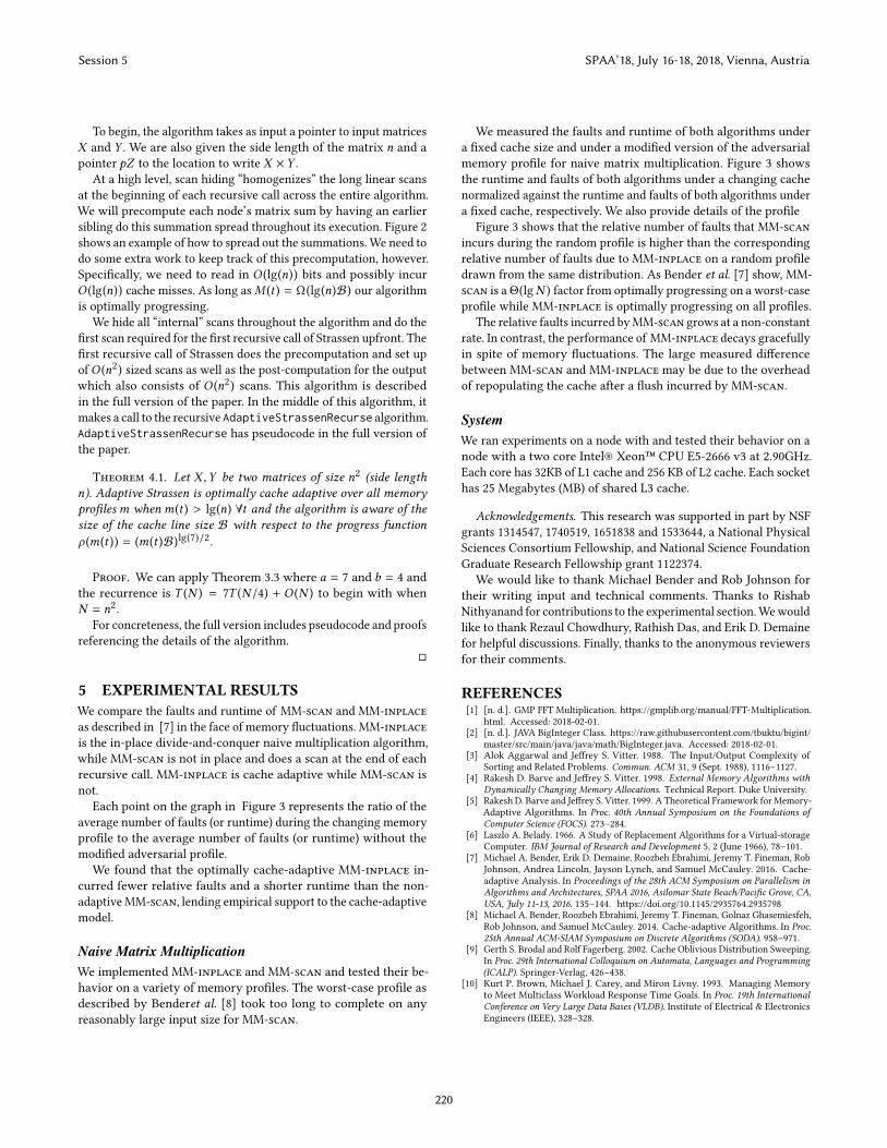
Each point on the graph in Figure 3 represents the ratio of the

average number of faults (or runtime) during the changing memory

profile to the average number of faults (or runtime) without the

modified adversarial profile.

We found that the optimally cache-adaptive MM-inplace in-

curred fewer relative faults and a shorter runtime than the non-

adaptiveMM-scan, lending empirical support to the cache-adaptive

model.

Naive Matrix MultiplicationWe implementedMM-inplace andMM-scan and tested their be-

havior on a variety of memory profiles. The worst-case profile as

described by Benderet al. [8] took too long to complete on any

reasonably large input size for MM-scan.

We measured the faults and runtime of both algorithms under

a fixed cache size and under a modified version of the adversarial

memory profile for naive matrix multiplication. Figure 3 shows

the runtime and faults of both algorithms under a changing cache

normalized against the runtime and faults of both algorithms under

a fixed cache, respectively. We also provide details of the profile

Figure 3 shows that the relative number of faults that MM-scan

incurs during the random profile is higher than the corresponding

relative number of faults due to MM-inplace on a random profile

drawn from the same distribution. As Bender et al. [7] show, MM-

scan is aΘ(lgN ) factor from optimally progressing on a worst-case

profile while MM-inplace is optimally progressing on all profiles.

The relative faults incurred byMM-scan grows at a non-constant

rate. In contrast, the performance of MM-inplace decays gracefully

in spite of memory fluctuations. The large measured difference

betweenMM-scan andMM-inplace may be due to the overhead

of repopulating the cache after a flush incurred by MM-scan.

SystemWe ran experiments on a node with and tested their behavior on a

node with a two core Intel® Xeon™ CPU E5-2666 v3 at 2.90GHz.

Each core has 32KB of L1 cache and 256 KB of L2 cache. Each socket

has 25 Megabytes (MB) of shared L3 cache.

Acknowledgements. This research was supported in part by NSF

grants 1314547, 1740519, 1651838 and 1533644, a National Physical

Sciences Consortium Fellowship, and National Science Foundation

Graduate Research Fellowship grant 1122374.

We would like to thank Michael Bender and Rob Johnson for

their writing input and technical comments. Thanks to Rishab

Nithyanand for contributions to the experimental section.Wewould

like to thank Rezaul Chowdhury, Rathish Das, and Erik D. Demaine

for helpful discussions. Finally, thanks to the anonymous reviewers

for their comments.

REFERENCES

[1] [n. d.]. GMP FFT Multiplication. https://gmplib.org/manual/FFT-Multiplication.

html. Accessed: 2018-02-01.

[2] [n. d.]. JAVA BigInteger Class. https://raw.githubusercontent.com/tbuktu/bigint/

master/src/main/java/java/math/BigInteger.java. Accessed: 2018-02-01.

[3] Alok Aggarwal and Jeffrey S. Vitter. 1988. The Input/Output Complexity of

Sorting and Related Problems. Commun. ACM 31, 9 (Sept. 1988), 1116–1127.

[4] Rakesh D. Barve and Jeffrey S. Vitter. 1998. External Memory Algorithms withDynamically Changing Memory Allocations. Technical Report. Duke University.

[5] Rakesh D. Barve and Jeffrey S. Vitter. 1999. A Theoretical Framework for Memory-

Adaptive Algorithms. In Proc. 40th Annual Symposium on the Foundations ofComputer Science (FOCS). 273–284.

[6] Laszlo A. Belady. 1966. A Study of Replacement Algorithms for a Virtual-storage

Computer. IBM Journal of Research and Development 5, 2 (June 1966), 78–101.[7] Michael A. Bender, Erik D. Demaine, Roozbeh Ebrahimi, Jeremy T. Fineman, Rob

Johnson, Andrea Lincoln, Jayson Lynch, and Samuel McCauley. 2016. Cache-

adaptive Analysis. In Proceedings of the 28th ACM Symposium on Parallelism inAlgorithms and Architectures, SPAA 2016, Asilomar State Beach/Pacific Grove, CA,USA, July 11-13, 2016. 135–144. https://doi.org/10.1145/2935764.2935798

[8] Michael A. Bender, Roozbeh Ebrahimi, Jeremy T. Fineman, Golnaz Ghasemiesfeh,

Rob Johnson, and Samuel McCauley. 2014. Cache-adaptive Algorithms. In Proc.25th Annual ACM-SIAM Symposium on Discrete Algorithms (SODA). 958–971.

[9] Gerth S. Brodal and Rolf Fagerberg. 2002. Cache Oblivious Distribution Sweeping.

In Proc. 29th International Colloquium on Automata, Languages and Programming(ICALP). Springer-Verlag, 426–438.

[10] Kurt P. Brown, Michael J. Carey, and Miron Livny. 1993. Managing Memory

to Meet Multiclass Workload Response Time Goals. In Proc. 19th InternationalConference on Very Large Data Bases (VLDB). Institute of Electrical & Electronics

Engineers (IEEE), 328–328.


220

https://gmplib.org/manual/FFT-Multiplication.html

https://gmplib.org/manual/FFT-Multiplication.html

https://raw.githubusercontent.com/tbuktu/bigint/master/src/main/java/java/math/BigInteger.java

https://raw.githubusercontent.com/tbuktu/bigint/master/src/main/java/java/math/BigInteger.java

https://doi.org/10.1145/2935764.2935798

Figure 2: The purple squares represent the scans on the rightmost path of the root. The orange squares represent the rightmost

path of the second child of root. The scans represented in orange will be completed before the recursive call for B is made.

The scans will be completed by the leaf nodes under A. We represent the look-ahead computations as the small squares in the

rectangle labeled Computations ahead of time.

1

10

100

5 6 7 8 9 10 1

10

100

1000

5 6 7 8 9 10 0.1

1

10

100

5 6 7 8 9 10 0.1

1

10

100

5 6 7 8 9 10

Normalized

Ratio

Matrix Dimension (2x )

Faults (p=1/N)

MM-INMM-SCAN

Times (p=1/N) Faults (p=10e-8) Times (p=10e-8)

Figure 3: An empirical comparison of faults and runtime of MM-scan and MM-inplace under memory fluctuations. Each

plot shows the normalized faults or runtime under a randomized version of the worst-case profile.

The first two plots show the faults and runtime during a random profile where the memory drops with probability p = 1/N at

the beginning of each recursive call.

Similarly, in the last two plots, we drop the memory with probability p = 5×10−8 at the beginning of each recursive call. Recall

that the theoretical worst-case profile drops the memory at the beginning of each recursive call.

[11] Erik D. Demaine. 2002. Cache-Oblivious Algorithms and Data Structures. LectureNotes from the EEF Summer School on Massive Data Sets 8, 4 (2002), 1–249.

[12] Dave Dice, Virendra J. Marathe, and Nir Shavit. 2014. Brief Announcement:

Persistent Unfairness Arising from Cache Residency Imbalance. In 26th ACMSymposium on Parallelism in Algorithms and Architectures, SPAA ’14, Prague, CzechRepublic - June 23 - 25, 2014. 82–83. https://doi.org/10.1145/2612669.2612703

[13] Matteo Frigo, Charles E. Leiserson, Harald Prokop, and Sridhar Ramachandran.

1999. Cache-Oblivious Algorithms. In Proc. 40th Annual Symposium on theFoundations of Computer Science (FOCS). 285–298.

[14] Matteo Frigo, Charles E. Leiserson, Harald Prokop, and Sridhar Ramachandran.

2012. Cache-Oblivious Algorithms. ACM Transactions on Algorithms 8, 1 (2012),4.

[15] Pieter Ghysels and Wim Vanroose. 2014. Hiding Global Synchronization Latency

in the Preconditioned Conjugate Gradient Algorithm. Parallel Comput. 40, 7(2014), 224 – 238. https://doi.org/10.1016/j.parco.2013.06.001 7th Workshop on

Parallel Matrix Algorithms and Applications.

[16] Goetz Graefe. 2013. A New Memory-Adaptive External Merge Sort. Private

communication.

[17] Richard T. Mills. 2004. Dynamic Adaptation to CPU and Memory Load in ScientificApplications. Ph.D. Dissertation. The College of William and Mary.

[18] Richard T. Mills, Andreas Stathopoulos, and Dimitrios S. Nikolopoulos. 2004.

Adapting to Memory Pressure from within Scientific Applications on Multipro-

grammed COWs. In Proc. 8th International Parallel and Distributed ProcessingSymposium (IPDPS). 71.

[19] Richard T.Mills, Chuan Yue, Andreas Stathopoulos, andDimitrios S. Nikolopoulos.

2007. Runtime and Programming Support for Memory Adaptation in Scientific

Applications via Local Disk and Remote Memory. Journal of Grid Computing 5, 2

(01 Jun 2007), 213–234. https://doi.org/10.1007/s10723-007-9075-7

[20] HweeHwa Pang, Michael J. Carey, and Miron Livny. 1993. Memory-Adaptive

External Sorting. In Proc. 19th International Conference on Very Large Data Bases(VLDB). Morgan Kaufmann, 618–629.

[21] HweeHwa Pang, Michael J Carey, and Miron Livny. 1993. Partially Preemptible

Hash Joins. In Proc. 5th ACM SIGMOD International Conference on Managementof Data (COMAD). 59.

[22] Daniel D. Sleator and Robert E. Tarjan. 1985. Amortized Efficiency of List Update

and Paging Rules. Commun. ACM 28, 2 (February 1985), 202–208.

[23] Volker Strassen. 1969. Gaussian Elimination is Not Optimal. Numer. Math. 13, 4(Aug. 1969), 354–356. https://doi.org/10.1007/BF02165411

[24] Volker Strumpen and Thomas L. Casavant. 1994. Exploiting Communication

Latency Hiding for Parallel Network Computing: Model and Analysis. In Proceed-ings of 1994 International Conference on Parallel and Distributed Systems. 622–627.https://doi.org/10.1109/ICPADS.1994.590409

[25] Jeffrey Scott Vitter. 2001. External memory algorithms and data structures:

dealing with massive data. Comput. Surveys 33, 2 (2001).[26] Jeffrey Scott Vitter. 2006. Algorithms and Data Structures for External Memory.

Foundations and Trends in Theoretical Computer Science 2, 4 (2006), 305–474.[27] Hansjörg Zeller and Jim Gray. 1990. An Adaptive Hash Join Algorithm for

Multiuser Environments. In Proc. 16th International Conference on Very LargeData Bases (VLDB). 186–197.

[28] Weiye Zhang and Per-Äke Larson. 1996. A Memory-Adaptive Sort (MASORT) for

Database Systems. In Proc. 6th International Conference of the Centre for AdvancedStudies on Collaborative research (CASCON). IBM Press, 41–.

[29] Weiye Zhang and Per-Äke Larson. 1997. Dynamic Memory Adjustment for

External Mergesort. In Proc. 23rd International Conference on Very Large DataBases (VLDB). Morgan Kaufmann Publishers Inc., 376–385.


221

https://doi.org/10.1145/2612669.2612703

https://doi.org/10.1016/j.parco.2013.06.001

https://doi.org/10.1007/s10723-007-9075-7

https://doi.org/10.1007/BF02165411

https://doi.org/10.1109/ICPADS.1994.590409

× =X11 X12

X21 X22

Y11 Y12

Y21 Y22

P1 + P2

T11 = X11

T12 = Y12 − Y22

T21 = X11 +X12

T22 = Y22

P1 = T11T12

P2 = T21T22

× = P1T11 T12 T21 T22 P2× =

Seven Mulitplications for P1 (dashed squares). Interspersed are additions (solid lines).

In the intial scan T11 and T12 will be pre-computed.

The matricies T21 and T22 must be computed before the mulitplication of P1 finishes.

X12

X × Y = Z

T11 × T12 = P1 T21 × T22 = P2

Larger Depiction Larger Depiction

T21 T21T22 T22 P2X11 X12 Y22

Figure 4: The pre-computation scan of size O (n2) would in this case pre-compute T11 and T21. Then, all multiplications can be

done. Assume that the smallest size of subproblem (3 small boxes) fit in memory. Then we show how the (dotted line boxes

not filled in) multiplications needed for P1 can be inter-spersed with the (complete line and colored in) additions or scans

needed to pre-compute T21 and T22. Note that T21 and T22 will be done computing before we try to compute the multiplication

of P2. Thus, we can repeat the process of multiplies interspersed with pre-computation during the multiplication for P2. Theadditions or scans during P2 will be for the inputs to the next multiplication, P3 (not listed here). The multiplications in P2 arecomputed based on the pre-computed matrices T21 and T22 (dotted line boxes filled in).


222

Cache-Adaptive Exploration: Experimental Results and Scan...

Documents

Transcript of Cache-Adaptive Exploration: Experimental Results and Scan...