C3 MEI A-level Maths Coursework

Maurice Yap 6946 – Core 3 Mathematics Coursework – 4752/02 Methods for Advanced Mathematics

Using numerical methods to find roots of and solve polynomial equationsThis report will explore and compare the advantages and disadvantages of three different numerical methods used to solve polynomial equations, where analytical methods cannot easily be used. It will explore instances where, for some reason, they fail and also examine their ease, efficiency and usefulness in solving polynomial equations.

Change of sign decimal search methodThe ‘change of sign’ method can be used to find an approximation of a root to an equation to a specified accuracy, using a decimal search.

Polynomial equations can be illustrated graphically as the function y = f(x), as shown below in figure 1. The points where the curve intersects the x-axis are the real roots of the equation f(x) =0, because the x-axis is where y = 0. If the curve crosses this line, the values for f(x) when x is slightly larger and smaller than the root will be positive and negative, either way round (given that the values chosen for x are not beyond any other roots).

A logical and systematic way to use this to solve an equation to a certain degree of accuracy is a decimal search, where having already identified integer intervals where roots occur, the interval is divided into ten, and f(x) for each of the ten new values for x is found. A search for a change of sign (+ or -) is conducted and the process is repeated in the interval where the change of sign occurs until the level of accuracy desired is achieved. After this, the same technique is applied to find the other roots and thereby solving the equation.

Example of an application of the change of sign methodFor example, consider solving the following equation, by first finding the greatest root to five significant figures:

6 x5−9 x4−4 x3−20 x+26=0

It is shown in figure 1 that there are three roots to this equation. That which is labelled ‘root c’ will be attempted to be found.

x f(x)-5 -23749-4 -8086-3 -1993-2 -238-1 350 261 -12 23 5874 3530

5 12551Table 1: integer search for changes in sign

From the changes in sign in table 1, (+, green rows or -, red rows), it can be seen that there are roots in the intervals (-2, -1), (0, 1) and (1, 2). These changes are shown as the blue rows of the table. The integer interval which contains root c can be deduced to be (1, 2). The integer search process of finding this interval is shown for the two bounds here:

f (1 )=6 (1 )5−9 (1 )4−4 (1 )3−20 (1 )+26=6−9−4−20+26=−1

f (2 )=6 (2 )5−9 (2 )4−4 (2 )3−20 (2 )+26=192−144−32−40+26=2

1


Figure 1: a graph of the function y = f(x), where f(x) = 6x5-9x4-4x3-20x+26

x f(x) x f(x) x f(x)1 -1 1.9 -8.15896 1.98 -0.385303859

1.1 -4.83784 1.91 -7.332245319 1.981 -0.2704782441.2 -8.64448 1.92 -6.465898701 1.982 -0.1551911061.3 -12.21532 1.93 -5.559037574 1.983 -0.0394414811.4 -15.28096 1.94 -4.610767706 1.984 0.0767715921.5 -17.5 1.95 -3.620183125 1.985 0.1934490771.6 -18.45184 1.96 -2.586366054 1.986 0.310591941.7 -17.62948 1.97 -1.508386836 1.987 0.4282011461.8 -14.43232 1.98 -0.385303859 1.988 0.5462776641.9 -8.15896 1.99 0.783836509 1.989 0.664822462

2 2 2 2 1.99 0.783836509

x is in the interval (1.9, 2) x is in the interval (1.98, 1.99) x is in the interval (1.983, 1.984)

x=2 to 1 significant figure x=1.9 to 2 significant figures x=1.98 to 3 significant figuresx=1.95±0.05 x=1.985±0.005 x=1.9835±0.0005

Table 2: the decimal search process, repeated until a result with an accuracy of 5 significant figures is achieved

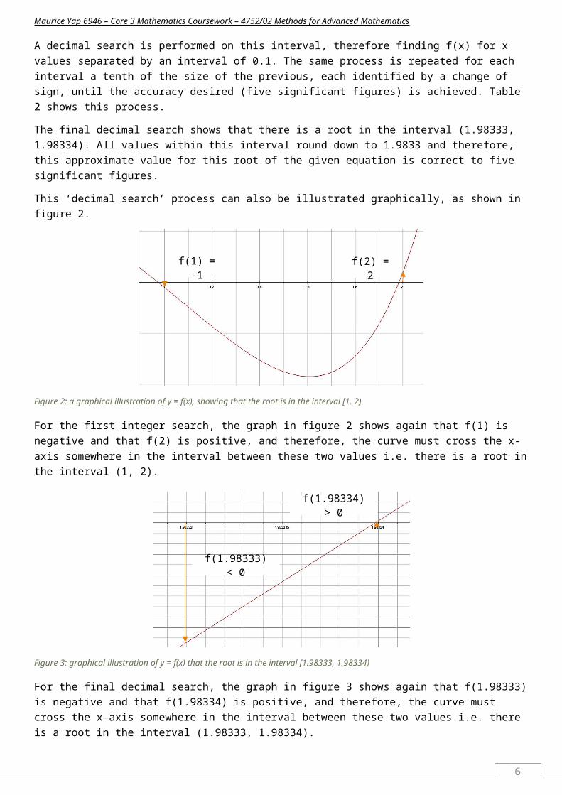
A decimal search is performed on this interval, therefore finding f(x) for x values separated by an interval of 0.1. The same process is repeated for each interval a tenth of the size of the previous, each identified by a change of sign, until the accuracy desired (five significant figures) is achieved. Table 2 shows this process.

2

Root c

Root b

Root a

x f(x) x f(x)1.983 -0.039441481 1.9833 -0.0046262651.9831 -0.027841045 1.98331 -0.0034650391.9832 -0.016235973 1.98332 -0.0023037671.9833 -0.004626265 1.98333 -0.0011424481.9834 0.00698808 1.98334 1.89167E-051.9835 0.018607064 1.98335 0.0011803281.9836 0.030230687 1.98336 0.0023417861.9837 0.041858951 1.98337 0.003503291.9838 0.053491855 1.98338 0.004664841.9839 0.065129402 1.98339 0.005826437

1.984 0.076771592 1.9834 0.00698808

x is in the interval (1.9833, 1.9834) x is in the interval (1.98333, 1.98334)

x=1.983 to 4 significant figures x=1.9833 to 5 significant figuresx=1.98335±0.00005 x=1.983335±0.000005


The final decimal search shows that there is a root in the interval (1.98333, 1.98334). All values within this interval round down to 1.9833 and therefore, this approximate value for this root of the given equation is correct to five significant figures.

This ‘decimal search’ process can also be illustrated graphically, as shown in figure 2.

For the first integer search, the graph in figure 2 shows again that f(1) is negative and that f(2) is positive, and therefore, the curve must cross the x-axis somewhere in the interval between these two values i.e. there is a root in the interval (1, 2).

For the final decimal search, the graph in figure 3 shows again that f(1.98333) is negative and that f(1.98334) is positive, and therefore, the curve must cross the x-axis somewhere in the interval between these two values i.e. there is a root in the interval (1.98333, 1.98334).

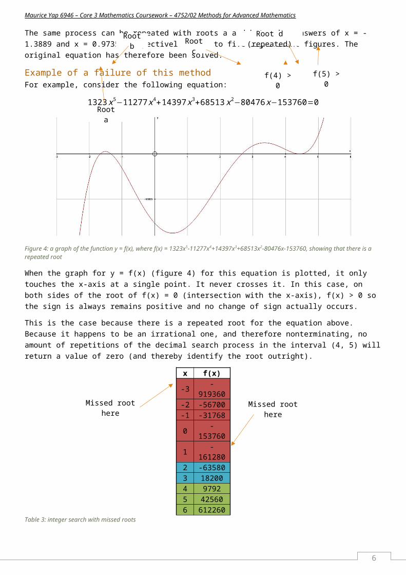
The same process can be repeated with roots a and b to give answers of x = -1.3889 and x = 0.97356 respectively, each to five significant figures. The original equation has therefore been solved.

Example of a failure of this methodFor example, consider the following equation:

1323 x5−11277 x4+14397 x3+68513 x2−80476 x−153760=0

f(2) = 2f(1) = -1

f(1.98333) < 0

f(1.98334) > 0

3

Figure 2: a graphical illustration of y = f(x), showing that the root is in the interval [1, 2)

Figure 3: graphical illustration of y = f(x) that the root is in the interval [1.98333, 1.98334)


Figure 4: a graph of the function y = f(x), where f(x) = 1323x5-11277x4+14397x3+68513x2-80476x-153760, showing that there is a repeated root

When the graph for y = f(x) (figure 4) for this equation is plotted, it only touches the x-axis at a single point. It never crosses it. In this case, on both sides of the root of f(x) = 0 (intersection with the x-axis), f(x) > 0 so the sign is always remains positive and no change of sign actually occurs.

This is the case because there is a repeated root for the equation above. Because it happens to be an irrational one, and therefore nonterminating, no amount of repetitions of the decimal search process in the interval (4, 5) will return a value of zero (and thereby identify the root outright).

x f(x)-3 -919360-2 -56700-1 -317680 -1537601 -1612802 -635803 182004 97925 425606 612260

Table 3: integer search with missed roots

Table 3 shows how an integer search suggests that there are just two roots in the interval searched. Not only does it show that the technique does not suggest that there is a root in the interval, (4, 5), it also does not show that there is a root in the interval (-2, -1) because there are two distinct roots occurring close together within the said interval, and both f(-2) and f(-1) are negative so it wouldn’t be seen to be necessary to conduct a decimal search on this interval.

The change of sign method fails here because it has failed to identify the root in the intervals (-2,-1) and (4, 5).

Newton-Raphson methodThis method works by taking an estimated root and finding where its tangent to the curve crosses the x-axis. The x-coordinate of this intersection is taken and its tangent to the curve is taken and the process is repeated. In most cases the x-coordinate becomes closer to the root with each repetition.

Taking x0 as the first rough estimate, the point on the curve for this x-value would be (x0, f(x0)). A general straight line can be written in the form

y− y0=m(x−x0)

The tangent to the curve, with the gradient being the derivative of f(x) at x0 (f’(x0)), would be expressed as the following function:

Missed root hereMissed root here

f(5) > 0

Root cRoot d (repeated)Root b

Root a

f(4) > 0

4


y−f ( x0 )=f ' ( x ) [ x−x0 ]The next x-coordinate will be called x1. It is where the line stated above crosses the x-axis, in other words, when y = 0. Substituting this into the function above, as well as changing x to x1 to make it the first iteration, it can be rearranged to give the following:

x1=x0−f (x0)f ' (x)

When this is generalised for when x0 = xn, the inductive formula is given as:

xn+1=xn−f (xn)f ' (xn)

Example of an application of the Newton-Raphson methodThe Newton-Raphson method will be used to solve the following equation:

x3+3 x2−13 x+4=0

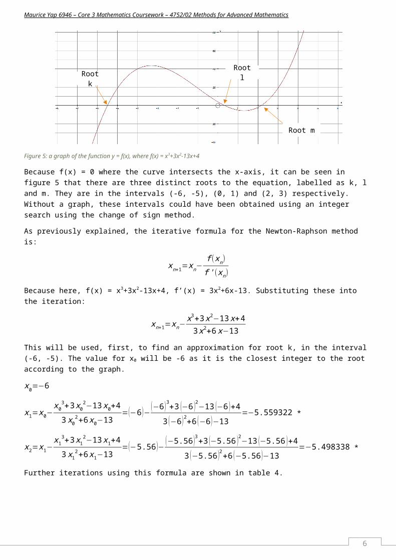
Figure 5: a graph of the function y = f(x), where f(x) = x3+3x2-13x+4

Because f(x) = 0 where the curve intersects the x-axis, it can be seen in figure 5 that there are three distinct roots to the equation, labelled as k, l and m. They are in the intervals (-6, -5), (0, 1) and (2, 3) respectively. Without a graph, these intervals could have been obtained using an integer search using the change of sign method.

As previously explained, the iterative formula for the Newton-Raphson method is:

xn+1=xn−f (xn)f ' (xn)

Because here, f(x) = x3+3x2-13x+4, f’(x) = 3x2+6x-13. Substituting these into the iteration:

xn+1=xn−x3+3 x2−13 x+4

3 x2+6 x−13

This will be used, first, to find an approximation for root k, in the interval (-6, -5). The value for x0 will be -6 as it is the closest integer to the root according to the graph.

x0=−6

x1=x0−x0

3+3 x02−13 x0+4

3 x02+6 x0−13

=(−6 )− (−6 )3+3 (−6 )2−13 (−6 )+4

3 (−6 )2+6 (−6 )−13=−5.559322 *

Root m

Root lRoot k

5


x2=x1−x1

3+3 x12−13 x1+4

3x12+6 x1−13

=(−5.56 )− (−5.56 )3+3 (−5.56 )2−13 (−5.56 )+4

3 (−5.56 )2+6 (−5.56 )−13=−5.498338 *

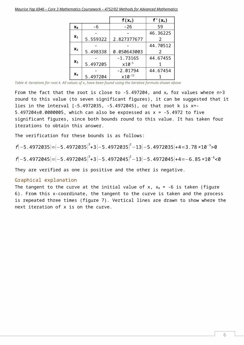
Further iterations using this formula are shown in table 4.

6


f(xn) f’(xn)

x0 -6 -26 59x1 -5.559322 -2.827377677 46.362252x2 -5.498338 -0.050643003 44.705122x3 -5.497205 -1.73165 x10-5 44.674551

x4 -5.497204 -2.01794 x10-12 44.674541Table 4: iterations for root k. All values of xn have been found using the iterative formula shown above

From the fact that the root is close to -5.497204, and xn for values where n>3 round to this value (to seven significant figures), it can be suggested that it lies in the interval [-5.4972035, -5.4972045), or that root k is x=-5.497204±0.0000005, which can also be expressed as x = -5.4972 to five significant figures, since both bounds round to this value. It has taken four iterations to obtain this answer.

The verification for these bounds is as follows:

f (−5.4972035 )=(−5.4972035 )3+3 (−5.4972035 )2−13 (−5.4972035 )+4=3.78 ×10−5>0

f (−5.4972045 )=(−5.4972045 )3+3 (−5.4972045 )2−13 (−5.4972045 )+4=−6.85 ×10−6<0

They are verified as one is positive and the other is negative.

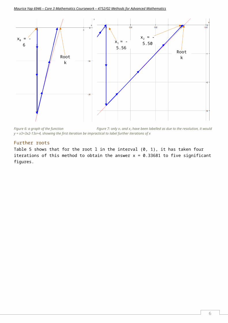
Graphical explanationThe tangent to the curve at the initial value of x, x0 = -6 is taken (figure 6). From this x-coordinate, the tangent to the curve is taken and the process is repeated three times (figure 7). Vertical lines are drawn to show where the next iteration of x is on the curve.

Figure 6: a graph of the function Figure 7: only x1 and x2 have been labelled as due to the resolution, it would y = x3+3x2-13x+4, showing the first iteration be impractical to label further iterations of x

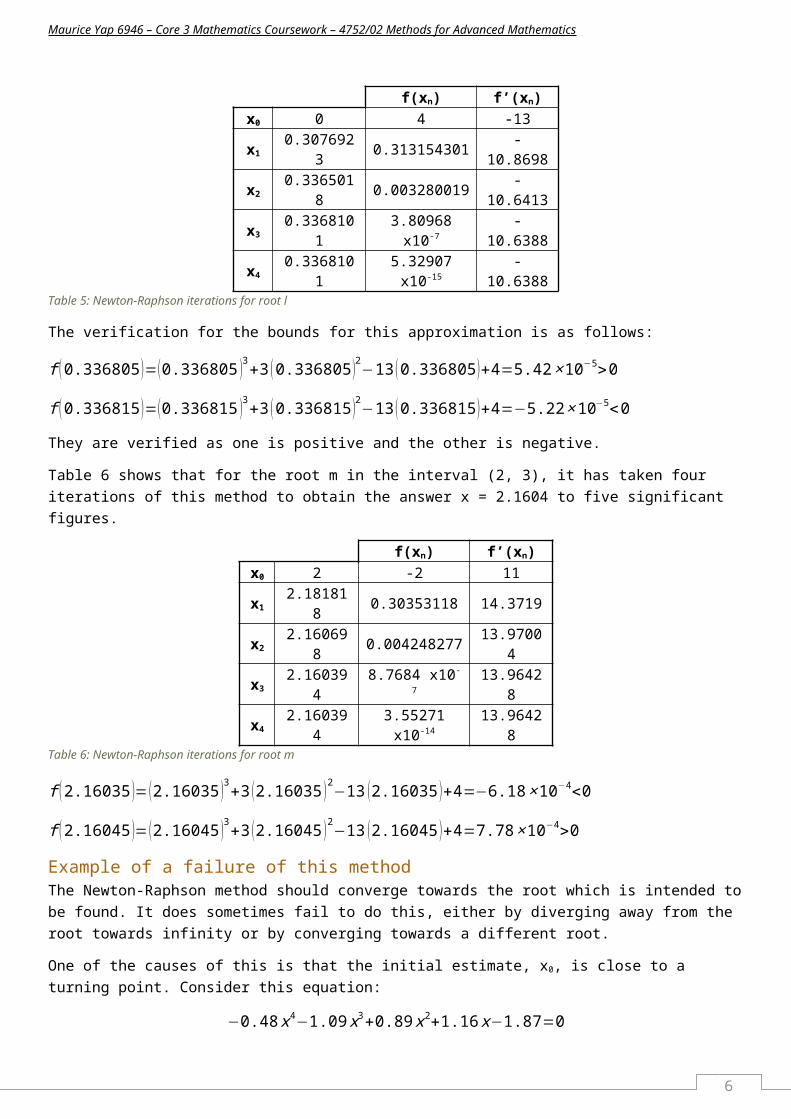
Further rootsTable 5 shows that for the root l in the interval (0, 1), it has taken four iterations of this method to obtain the answer x = 0.33681 to five significant figures.

Root k

x0 = -6 x2 ≈ -5.50x1 ≈ -5.56

Root k

7


f(xn) f’(xn)

x0 0 4 -13x1 0.3076923 0.313154301 -10.8698x2 0.3365018 0.003280019 -10.6413x3 0.3368101 3.80968 x10-7 -10.6388

x4 0.3368101 5.32907 x10-15 -10.6388Table 5: Newton-Raphson iterations for root l

The verification for the bounds for this approximation is as follows:

f (0.336805 )=(0.336805 )3+3 (0.336805 )2−13 (0.336805 )+4=5.42 ×10−5>0

f (0.336815 )=(0.336815 )3+3 (0.336815 )2−13 (0.336815 )+4=−5.22×10−5<0


Table 6 shows that for the root m in the interval (2, 3), it has taken four iterations of this method to obtain the answer x = 2.1604 to five significant figures.

f(xn) f’(xn)

x0 2 -2 11x1 2.181818 0.30353118 14.3719x2 2.160698 0.004248277 13.97004x3 2.160394 8.7684 x10-7 13.96428

x4 2.160394 3.55271 x10-14 13.96428Table 6: Newton-Raphson iterations for root m

f (2.16035 )=(2.16035 )3+3 (2.16035 )2−13 (2.16035 )+4=−6.18 ×10−4<0

f (2.16045 )=(2.16045 )3+3 (2.16045 )2−13 (2.16045 )+4=7.78×10−4>0

Example of a failure of this methodThe Newton-Raphson method should converge towards the root which is intended to be found. It does sometimes fail to do this, either by diverging away from the root towards infinity or by converging towards a different root.

One of the causes of this is that the initial estimate, x0, is close to a turning point. Consider this equation:

−0.48 x4−1.09x3+0.89 x2+1.16x−1.87=0

Figure 8: a graph of the function y = f(x), where f(x) = −0.48x4−1.09x3+0.89x2+1.16x−1.87=0

Root e

Root d

8


Figure 8 shows that there are two roots to this equation. The Newton-Raphson method will be applied to try to find root d with an estimate by eye of x0 = -2.

The iteration formula is given by the following:

xn+1=xn−−0.48 x4−1.09 x3+0.89 x2+1.16 x−1.87

−1.92 x3−3.27 x2+1.78 x+1.16

Table 7 shows eighteen iterations of x in a tabular format.

f(x) f'(x)

x0 -2 0.41 -0.12x1 1.4166667 -3.472899 -8.33993x2 1.0002484 -1.390559 -2.25261x3 0.3829392 -1.36681 1.254293x4 1.4726444 -3.970262 -9.44218x5 1.0521629 -1.52211 -2.8236x6 0.5130953 -1.221009 0.953072x7 1.7942253 -8.193961 -17.2632x8 1.3195768 -2.749496 -6.59684x9 0.9027871 -1.218257 -1.31089x10 -0.026547 -1.900147 1.110478x11 1.6845599 -6.466232 -14.2992x12 1.2323494 -2.235909 -5.2059x13 0.8028538 -1.128521 -0.51228x14 -1.400101 -0.602357 -2.47268x15 -1.643706 -0.035315 -2.07403x16 -1.660733 -0.00045 -2.02059x17 -1.660956 -8.04 x10-8 -2.01986x18 -1.660956 -2 x10-15 -2.01986

Table 7

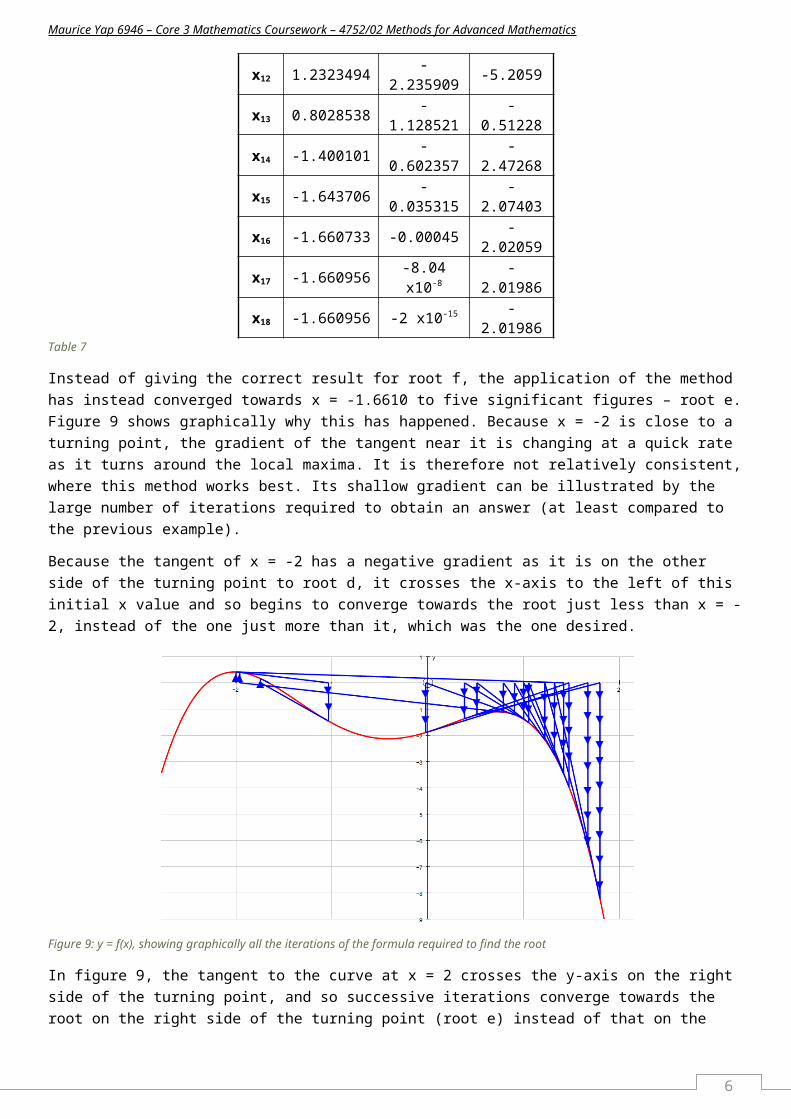
Instead of giving the correct result for root f, the application of the method has instead converged towards x = -1.6610 to five significant figures – root e. Figure 9 shows graphically why this has happened. Because x = -2 is close to a turning point, the gradient of the tangent near it is changing at a quick rate as it turns around the local maxima. It is therefore not relatively consistent, where this method works best. Its shallow gradient can be illustrated by the large number of iterations required to obtain an answer (at least compared to the previous example).

Because the tangent of x = -2 has a negative gradient as it is on the other side of the turning point to root d, it crosses the x-axis to the left of this initial x value and so begins to converge towards the root just less than x = -2, instead of the one just more than it, which was the one desired.

9


Figure 9: y = f(x), showing graphically all the iterations of the formula required to find the root

In figure 9, the tangent to the curve at x = 2 crosses the y-axis on the right side of the turning point, and so successive iterations converge towards the root on the right side of the turning point (root e) instead of that on the left (root d). This is what causes the failure for finding root d, with x0 = -2.

Rearrangement into x = g(x) methodThis method works by rearranging the equation f(x) = 0 into another where x is the subject, x = g(x). An iterative formula derived from this is then applied to this new function:

xn+1=g ( xn )

The application of this produces a converging sequence of numbers towards the value at which the line y = x crosses y = g(x) on a graph. Algebraically, this, through simultaneously solving through equating these two equations, gives, at the point where x = g(x), the x value for which f(x) = 0. It therefore finds the root.

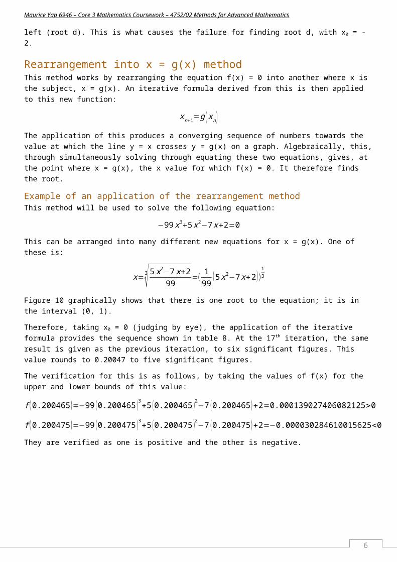
Example of an application of the rearrangement methodThis method will be used to solve the following equation:

−99 x3+5 x2−7x+2=0

This can be arranged into many different new equations for x = g(x). One of these is:

x=3√ 5 x2−7 x+299

=( 199

(5 x2−7 x+2 ))13

Figure 10 graphically shows that there is one root to the equation; it is in the interval (0, 1).

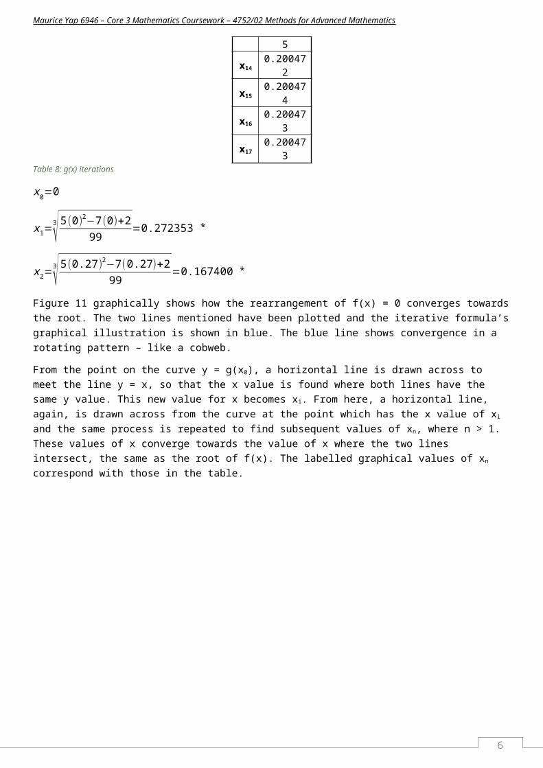
Therefore, taking x0 = 0 (judging by eye), the application of the iterative formula provides the sequence shown in table 8. At the 17th iteration, the same result is given as the previous iteration, to six significant figures. This value rounds to 0.20047 to five significant figures.

The verification for this is as follows, by taking the values of f(x) for the upper and lower bounds of this value:

f (0.200465 )=−99 (0.200465 )3+5 (0.200465 )2−7 (0.200465 )+2=0.000139027406082125>0

f (0.200475 )=−99 (0.200475 )3+5 (0.200475 )2−7 (0.200475 )+2=−0.000030284610015625<0


10


Figure 10: a graph of the function y = f(x), where f(x) = -99x3+5x2-7x+2

x0 0.000000x1 0.272353x2 0.167400x3 0.213859x4 0.194787x5 0.202838x6 0.199481x7 0.200888x8 0.200300x9 0.200546x10 0.200443x11 0.200486x12 0.200468x13 0.200475x14 0.200472x15 0.200474x16 0.200473

x17 0.200473Table 8: g(x) iterations

x0=0

x1=3√ 5 (0)2−7(0)+2

99=0.272353 *

x2=3√ 5 (0.27)2−7(0.27)+2

99=0.167400 *

Root

11


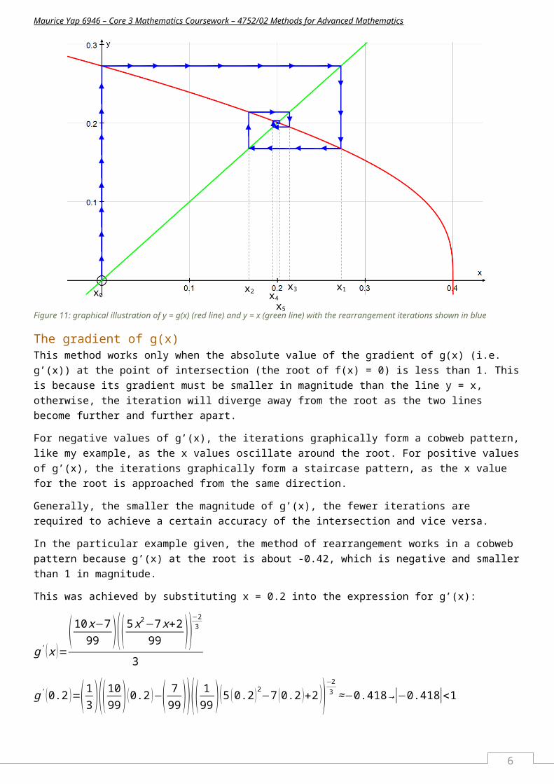
Figure 11 graphically shows how the rearrangement of f(x) = 0 converges towards the root. The two lines mentioned have been plotted and the iterative formula’s graphical illustration is shown in blue. The blue line shows convergence in a rotating pattern – like a cobweb.

From the point on the curve y = g(x0), a horizontal line is drawn across to meet the line y = x, so that the x value is found where both lines have the same y value. This new value for x becomes x1. From here, a horizontal line, again, is drawn across from the curve at the point which has the x value of x1 and the same process is repeated to find subsequent values of xn, where n > 1. These values of x converge towards the value of x where the two lines intersect, the same as the root of f(x). The labelled graphical values of xn correspond with those in the table.

Figure 11: graphical illustration of y = g(x) (red line) and y = x (green line) with the rearrangement iterations shown in blue

The gradient of g(x)This method works only when the absolute value of the gradient of g(x) (i.e. g’(x)) at the point of intersection (the root of f(x) = 0) is less than 1. This is because its gradient must be smaller in magnitude than the line y = x, otherwise, the iteration will diverge away from the root as the two lines become further and further apart.

For negative values of g’(x), the iterations graphically form a cobweb pattern, like my example, as the x values oscillate around the root. For positive values of g’(x), the iterations graphically form a staircase pattern, as the x value for the root is approached from the same direction.

Generally, the smaller the magnitude of g’(x), the fewer iterations are required to achieve a certain accuracy of the intersection and vice versa.

In the particular example given, the method of rearrangement works in a cobweb pattern because g’(x) at the root is about -0.42, which is negative and smaller than 1 in magnitude.

This was achieved by substituting x = 0.2 into the expression for g’(x):

g' (x )=(10 x−7

99 )((5 x2−7 x+299 ))

−23

3

g' (0.2 )=( 13 )(( 10

99 )( 0.2 )−( 799 ))(( 1

99 ) (5 (0.2 )2−7 (0.2 )+2 ))−23 ≈−0.418 →|−0.418|<1

x0x1x2 x3

x5

12

x4


Failure of this methodAnother way of rearranging the equation f(x) = 0 is shown below. This equation will be referred to as x = h(x).

x=−99 x3+5 x2+27

As an iterative formula, this is:

xn+1=−99 xn

3+5 xn2+2

7

Table 9 shows iterations of this formula, again starting with x0 = 0. It can be deduced that xn does not find the root because the values seem to reoccur from the seventh and eighth iterations onwards, according to this degree of accuracy.

Figure 12 graphically illustrates this failure, showing that the first couple of iterations form a cobweb pattern, but then goes round and round on itself, forming a stationary rectangle. This is the observation that the values for each iteration of xn change from 0.013857 and 0.285814 and keep doing so, seemingly forever.

x0 0

x1 0.285714

x2 0.014161

x3 0.285817

x4 0.013846

x5 0.285814

x6 0.013857

x7 0.285814

x8 0.013857

x9 0.285814

x10 0.013857

x11 0.285814

⁞ ⁞

x1428 0.013857

x1429 0.285814

x1430 0.013857

x1431 0.285814Table 9: h(x) iterations

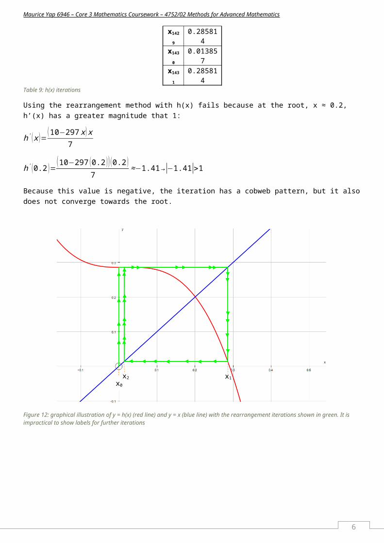
Using the rearrangement method with h(x) fails because at the root, x ≈ 0.2, h’(x) has a greater magnitude that 1:

h' ( x )= (10−297 x ) x7

h' (0.2 )=(10−297 (0.2 ) ) (0.2 )

7≈−1.41→|−1.41|>1

Because this value is negative, the iteration has a cobweb pattern, but it also does not converge towards the root.

13


Figure 12: graphical illustration of y = h(x) (red line) and y = x (blue line) with the rearrangement iterations shown in green. It is impractical to show labels for further iterations

14

x0

x1x2


Comparison of the methodsComparative application of all three methodsI will use the three methods explored to find the root of the equation, 6x5-9x4-4x3-20x+26 = 0 in the interval (-2, -1).

Change of sign decimal search methodThe decimal search finds that the root is between the values -1.388863 and -1.388862 and so x = -1.3889, correct to five significant figures. This took six iterations since bounds of seven significant figures are required to ensure an accuracy of five significant figures. Table 10 shows these iterations.

x f(x) x f(x) x f(x)-2 -238 -1.4 -1.86784 -1.39 -0.187924509

-1.9 -174.41884 -1.39 -0.187924509 -1.389 -0.022685742-1.8 -122.52448 -1.38 1.442231859 -1.388 0.142056416-1.7 -80.70832 -1.37 3.023594836 -1.387 0.306302934-1.6 -47.51296 -1.36 4.557118054 -1.386 0.47005478-1.5 -21.625 -1.35 6.043743125 -1.385 0.633312923-1.4 -1.86784 -1.34 7.484399706 -1.384 0.796078328-1.3 12.80552 -1.33 8.880005574 -1.383 0.958351961-1.2 23.31968 -1.32 10.2314667 -1.382 1.120134786-1.1 30.48404 -1.31 11.53967732 -1.381 1.281427764-1 35 -1.3 12.80552 -1.38 1.442231859

x f(x) x f(x) x f(x)-1.389 -0.022685742 -1.3889 -0.006189195 -1.38887 -0.001241199-1.3889 -0.006189195 -1.38889 -0.004539813 -1.388869 -0.001076273-1.3888 0.010302388 -1.38888 -0.002890481 -1.388868 -0.000911348-1.3887 0.026789005 -1.38887 -0.001241199 -1.388867 -0.000746424-1.3886 0.04327066 -1.38886 0.000408034 -1.388866 -0.0005815-1.3885 0.059747353 -1.38885 0.002057217 -1.388865 -0.000416576-1.3884 0.076219084 -1.38884 0.00370635 -1.388864 -0.000251653-1.3883 0.092685855 -1.38883 0.005355434 -1.388863 -8.67305E-05-1.3882 0.109147667 -1.38882 0.007004468 -1.388862 7.81915E-05-1.3881 0.12560452 -1.38881 0.008653453 -1.388861 0.000243113-1.388 0.142056416 -1.3888 0.010302388 -1.38886 0.000408034

Table 10: decimal search iterations for f(x)

Newton-Raphson methodUsing x0 = -1, the Newton-Raphson method takes seven iterations to find the same result to five significant figures, shown in table 11.

x0 -1x1 -2.029411765x2 -1.679330827x3 -1.473319358x4 -1.398239983x5 -1.38899275x6 -1.3888625

x7 -1.388862474Table 11: iterations to solve the chosen root of f(x) using the Newton-Raphson formula

15


Because Newton-Raphson does not give an interval which the root is in, it is necessary to verify the assumed result. This is shown below, using the interval bounds for the approximation of x = -1.3889 to 5 significant figures.

f (−1.38885 )=0.002057217>0

f (−1.38895 )=−0.0144368<0

Rearrangement into x = g(x) methodA rearrangement of f(x) as an iterative formula is the following:

xn+1=( 9 xn4+4 xn

3+20 xn−266 )

15

Iterations are shown in table 12. The root is shown to be x = -1.3889 to five significant figures.

x0 -1x1 -1.46868x2 -1.34256x3 -1.40875x4 -1.37891x5 -1.39351x6 -1.38662x7 -1.38993x8 -1.38835x9 -1.38911x10 -1.38875x11 -1.38892x12 -1.38884x13 -1.38888

x14 -1.38886Table 12: x = g(x) iterations

Again, for the same reasons as for the Newton-Raphson method, this answer must be verified using the upper and lower bounds of the approximation interval.

f (−1.38885 )=0.002057217>0

f (−1.38895 )=−0.0144368<0

Speed and efficiency comparisonIn order to produce the same approximation with the same accuracy for the chosen root, in this particular case, the decimal search method required the least number of iterations, with six needed. It required the highest number of single calculations.

The Newton-Raphson method required seven iterations. It was the method requiring the least number of single calculations.

The most iterations taken was the rearrangement method, with 14 needed.

In terms of speed, using spreadsheet software, the Newton-Raphson is quickest. On spreadsheet software, it requires an x0 value, a spreadsheet formula for f(x), a spreadsheet formula for f’(x) and a very simple iteration spreadsheet formula to be manually inputted. The differentiation is usually quite simple because each term of x has a positive, whole number power.

The rearrangement method took longer to converge and it can often take a large number of iterations to converge to an accuracy of five significant figures. Rearrangement is also quite easy and quick to do.

16


The decimal search was the slowest in finding the roots. Although it only took six iterations, without extremely complex spreadsheet formulas, each iteration needed to be set up individually on spreadsheet software through identifying the two bounds from the previous iteration. Simple and reliable though this method is, it is much more time-consuming than the other two methods. Each iteration also included nine unique calculations involving x.

TechnologiesSoftware-based spreadsheetUsing spreadsheet software like Google Docs Spreadsheet, Microsoft Excel or Numbers, all three methods are quite easy and quick to apply. Spreadsheets have the ability to quickly copy formulas and reapply them in a very short amount of time. This is done by keyboard shortcuts, context menus or by dragging or double clicking a cell’s fill handle. They can also be made to make the processes automatic through the use of complex spreadsheet formulas, a very strong advantage for bulk calculations of roots of equations. A disadvantage is that all mathematical formulas must be typed in using a non-dedicated QWERTY keyboard on desktops and laptops, which can be very clunky and tedious. This is even worse on tablets and smartphones, where the user must scroll through many pages of symbols on their keyboard to find commonly used mathematical symbols.

Using purely software-based spreadsheets, the decimal search method is easiest to use as it does not require any sort of mathematical calculation, like rearranging or differentiating, just simply typing in a spreadsheet formula for the function f(x).

Scientific calculatorIterative methods, like Newton-Raphson or rearranging for x = g(x), can be easily done on scientific calculators using the ‘answer’ button, or equivalent. A formula can be typed in, replacing xn with the ‘answer’ button, and pressing the ‘equals’ button gives the result for the next iteration.

The decimal search can, at a push, also be used, but it would take a very long time a very many button presses, because each calculation for f(x) must be typed in separately – nine separate polynomial calculations for each iteration.

A disadvantage of using a scientific calculator is the fact that the small display and linear input makes it easy to forget to close brackets, resulting in an error.

Newton-Raphson is, in my opinion, the easiest method to use with just a scientific calculator as it is iterative and the calculation would normally be relatively straightforward to work out and type in.

Graphical calculatorIn the same way as scientific calculators, iterative formulas are easy to apply using graphical calculators. Some also have the advantage of being able to differentiate with respect to a variable like ‘x’, meaning the user doesn’t have to if they are lazy.

Iterative formulas can also be put into tables, much like a spreadsheet. This makes it easier to spot convergence. Using the table calculator function, the decimal search can also easily be used.

I consider the decimal search the easiest method to use because it is easiest to type in just a simple polynomial equation, as opposed to complex iterative formulas of the other two methods.

Graphing softwareAdvanced graphing software like Autograph can be used to apply the Newton-Raphson and rearrangement methods in a graphical way.

For Newton-Raphson, Autograph requires for the graph of y = f(x) to be selected, then bringing up the context menu and selecting the Newton-Raphson option brings up a dialog box. This enables iterations of the formula to be plotted with an x0 value.

The x = g(x) method can be graphically plotted in the same way, but first, the line y = x must be plotted.

In my opinion, both these methods are equally easy to apply using Autograph software, but the Newton-Raphson method is the most reliable, so it would probably be my preference.

17


* For presentation purposes, the values printed are rounded, and not exact values. Subsequent uses of this number are shown rounded further, however, unrounded exact results have been used in the calculations.

18

C3 MEI A-level Maths Coursework

Documents

Transcript of C3 MEI A-level Maths Coursework