C HAPTER 11 The Transportation Problem 11 The Transportation Problem ... which mean that the numbers...
56
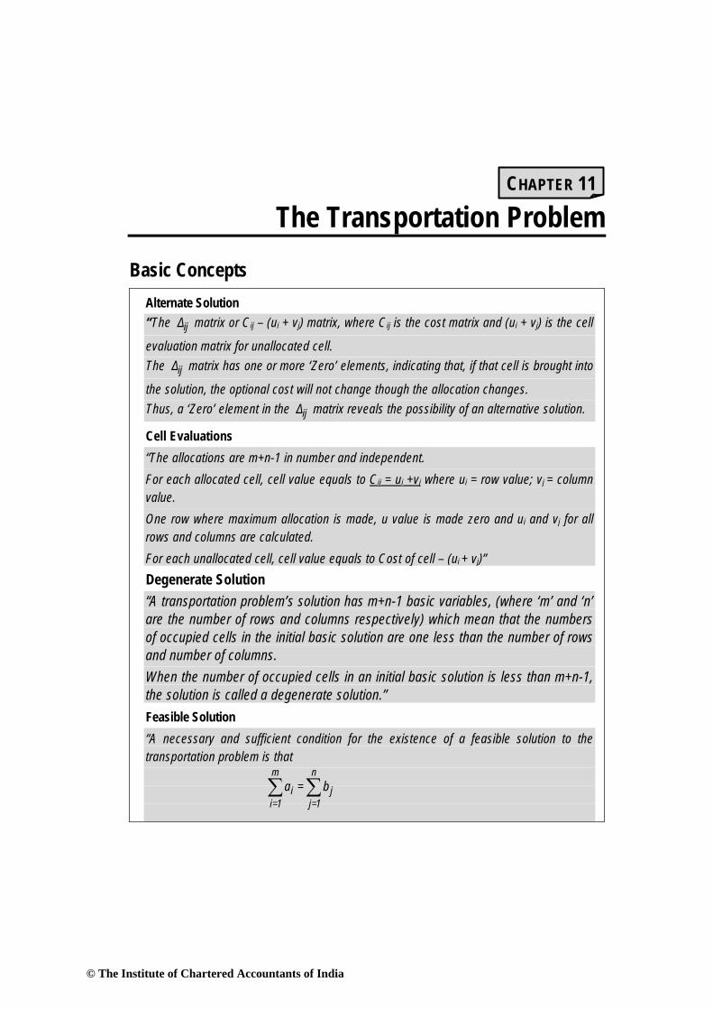
CHAPTER 11 The Transportation Problem Basic Concepts Alternate Solution “The ij Δ matrix or C ij – (u i + v j ) matrix, where C ij is the cost matrix and (u i + v j ) is the cell evaluation matrix for unallocated cell. The ij Δ matrix has one or more ‘Zero’ elements, indicating that, if that cell is brought into the solution, the optional cost will not change though the allocation changes. Thus, a ‘Zero’ element in the ij Δ matrix reveals the possibility of an alternative solution. Cell Evaluations “The allocations are m+n-1 in number and independent. For each allocated cell, cell value equals to C ij = u i +v j where u i = row value; v j = column value. One row where maximum allocation is made, u value is made zero and u i and v j for all rows and columns are calculated. For each unallocated cell, cell value equals to Cost of cell – (u i + v j )” Degenerate Solution “A transportation problem’s solution has m+n-1 basic variables, (where ‘m’ and ‘n’ are the number of rows and columns respectively) which mean that the numbers of occupied cells in the initial basic solution are one less than the number of rows and number of columns. When the number of occupied cells in an initial basic solution is less than m+n-1, the solution is called a degenerate solution.” Feasible Solution “A necessary and sufficient condition for the existence of a feasible solution to the transportation problem is that ∑ ∑ m n i j i =1 j =1 a= b © The Institute of Chartered Accountants of India
Transcript of C HAPTER 11 The Transportation Problem 11 The Transportation Problem ... which mean that the numbers...
CHAPTER 11
The Transportation Problem Basic Concepts
Alternate Solution “The ijΔ matrix or Cij – (ui + vj) matrix, where Cij is the cost matrix and (ui + vj) is the cell
evaluation matrix for unallocated cell. The ijΔ matrix has one or more ‘Zero’ elements, indicating that, if that cell is brought into
the solution, the optional cost will not change though the allocation changes. Thus, a ‘Zero’ element in the ijΔ matrix reveals the possibility of an alternative solution.
Cell Evaluations “The allocations are m+n-1 in number and independent. For each allocated cell, cell value equals to Cij = ui +vj where ui = row value; vj = column value. One row where maximum allocation is made, u value is made zero and ui and vj for all rows and columns are calculated. For each unallocated cell, cell value equals to Cost of cell – (ui + vj)” Degenerate Solution “A transportation problem’s solution has m+n-1 basic variables, (where ‘m’ and ‘n’ are the number of rows and columns respectively) which mean that the numbers of occupied cells in the initial basic solution are one less than the number of rows and number of columns. When the number of occupied cells in an initial basic solution is less than m+n-1, the solution is called a degenerate solution.” Feasible Solution “A necessary and sufficient condition for the existence of a feasible solution to the transportation problem is that
∑ ∑m n
i ji=1 j=1
a = b
© The Institute of Chartered Accountants of India
11.2 Advanced Management Accounting
Where ai = quantity of product available at origin i bj = quantity of product available at origin j In other words, the total capacity (or supply) must equal total requirement (or demand).”
North - West Corner Rule “This method simply consists of making allocations to each row in turn, apportioning as much as possible to its first cell and proceeding in this manner to its following cells until the row total in exhausted.” Optimality Test “Once the initial basic feasible solution is done, we have to do the optimality test. If it satisfy the condition that number of allocation is equal to (m+n-1) where m= number of rows, n= number of columns. If allocation is less than (m+n-1), then the problem shows degenerate situation. In that case we have to allocate an infinitely small quantity (e) in least cost and independent cell.”
Steps - North-West Corner Rule Step-1: “Before allocation ensure that the total of demand & supply of availability and requirement are equal. If not then make same equal by introducing dummy availability or requirement.”
Step-2: “The first allocation is made in the cell occupying the upper left hand corner of the matrix. The assignment is made in such a way that either the resource availability is exhausted or the demand at the first destination is satisfied.”
Step-3(a): “If the resource availability of the row one is exhausted first, we move down the second row and first column to make another allocation which either exhausts the resource availability of row two or satisfies the remaining destination demand of column one.
Step-3(b): “If the first allocation completely satisfies the destination demand of column one, we move to column two in row one, and make a second allocation which either exhausts the remaining resource availability of row one or satisfies the destination requirement under column two.”
Step-4: “The above procedure is repeated until all the row availability and column requirements are satisfied.”
Steps - The Least Cost Method Step-1: “Before starting the process of allocation ensure that the total of availability and
© The Institute of Chartered Accountants of India
The Transportation Problem 11.3
demand is equal. The least cost method starts by making the first allocation in the cell whose shipping cost (or transportation cost) per unit is lowest.”
Step-2: “This lowest cost cell is loaded or filled as much as possible in view of the origin capacity of its row and the destination requirements of its column.”
Step-3: “We move to the next lowest cost cell and make an allocation in view of the remaining capacity and requirement of its row and column. In case there is a tie for the lowest cost cell during any allocation, we can exercise our judgment and we arbitrarily choose cell for allocation.”
Step-4: “The above procedure is repeated till all row requirements are satisfied.”
Steps - Vogel’s Approximation Method (VAM) Step-1: “Before allocation ensure that the total of demand & supply of availability and requirement are equal. If not then make same equal by introducing dummy availability or requirement.” Step-2: “For each row of the transportation table identify the smallest and next smallest costs. Find the difference between the two costs and display it to the right of that row as “Difference” (Diff.). Likewise, find such a difference for each column and display it below that column. In case two cells contain the same least cost then the difference will be taken as ‘zero’.” Step-3: “From amongst these row and column differences, select the one with the largest difference. Allocate the maximum possible to the least cost cell in the selected column or row. If there occurs a tie amongst the largest differences, the choice may be made for a row or column which has least cost. In case there is a tie in cost cell also, choice may be made for a row or column by which maximum requirement is exhausted. Match that column or row containing this cell whose totals have been exhausted so that this column or row is ignored in further consideration.” Step-4: “Re-compute the column and row differences for the reduced transportation table and go to step 2. Repeat the procedure until all the column and row totals are exhausted.” Transportation Problem “This type of problem deals with optimization of transportation cost in a distribution scenario involving ‘m’ factories (sources) to ‘n’ warehouses (destination) where cost of shipping from ith factory to jth warehouse is given and goods produced at different factories and requirement at different warehouses are given.”
© The Institute of Chartered Accountants of India
11.4 Advanced Management Accounting
Prohibited Routes “Sometimes in a given transportation problem, some routes may not be available. There could be several reasons for this such as bad road conditions or strike etc. In such situations, there is a restriction on the route available for transportation. To handle such type of a situation, a very large cost (or a negative profit for the maximization problem) represented by ∞ or ‘M’ is assigned to each of such routes which are not available. Due to assignment of very large cost, such routes would automatically be eliminated in the final solution. The problem is the solved in its usual way.”
© The Institute of Chartered Accountants of India
© The Institute of Chartered Accountants of India
11.6 Advanced Management Accounting
Question-1 State the methods in which initial feasible solution can be arrived at in a transportation problem.
Solution:
The methods by which initial feasible solution can be arrived at in a transportation model are as under: (i) North-West Corner Method (ii) Least Cost Method (iii) Vogel’s Approximation Method (VAM) Question-2 How do you know whether an alternative solution exists for a transportation problem?
Solution:
The Δ ij matrix or Cij – (ui + vj) matrix, where Cij is the cost matrix and (ui + vj) is the cell evaluation matrix for unallocated cell. The Δ ij matrix has one or more ‘Zero’ elements, indicating that, if that cell is brought into the solution, the optional cost will not change though the allocation changes. Thus, a ‘Zero’ element in the Δ ij matrix reveals the possibility of an alternative solution. Question-3 Explain the term degeneracy in a transportation problem.
Solution:
A transportation problem’s solution has m+n-1 basic variables, (where ‘m’ and ‘n’ are the number of rows and columns respectively) which means that the number of occupied cells in the initial basic solution are one less than the number of rows and number of columns.
© The Institute of Chartered Accountants of India
The Transportation Problem 11.7
When the number of occupied cells in a initial basic solution are less than m+n-1, the solution is called a degenerate solution. Such a situation is handled by introducing an infinitesimally small allocation ‘e’ in the least cost and independent cell. If the number of occupied cells < m+n-1 by one, then only one ‘e’ needs to be introduced. If the number of occupied cells is less by more than one, to the extent of shortage, ‘e’‘s will have to be introduced till the condition that number of occupied cells = m+n-1. For example if number of occupied cells in an initial basic solution are 7 and we have m+n-1 (= 9), then, we have to introduce two quantities of ‘e’, say e1 and e2 in two of the least cost independent cells. Degeneracy occurs because in any particular allocation (earlier than the last allocation), the row and column totals get simultaneously fulfilled. (In the last allocation, it is always that row and column get fulfilled). Then, we have degeneracy by one number, i.e. number of occupied cells +1 equals m+n-1. We need to put one ‘e’. In the subsequent allocation, if again row and column totals get fulfilled simultaneously, again there will be a shortage of occupied cells and another ‘e’ will be required. Question-4 Will the initial solution for a minimization problem obtained by Vogel’s Approximation Method and the Least Cost Method be the same? Why?
Solution:
The initial solution need not be the same under both methods. Vogel’s Approximation Method uses the differences between the minimum and the next minimum costs for each row and column. This is the penalty or opportunity cost of not utilising the next best alternative. The highest penalty is given the 1st preference. This need not be the lowest cost. For example if a row has minimum cost as 3, and the next minimum as 2, penalty is 1; whereas if another row has minimum 4 and next minimum 6, penalty is 2, and this row is given preference. But Least Cost Method gives preference to the lowest cost cell, irrespective of the next cost. Solution obtained using Vogel’s Approximation Method is more optimal than Least Cost Method. Initial solution will be same only when the maximum penalty and the minimum cost coincide.
© The Institute of Chartered Accountants of India
11.8 Advanced Management Accounting
Question-5 In a transportation problem for cost minimization, there are 4 rows indicating quantities demanded and this totals up to 1,200 units. There are 4 columns giving quantities supplied. This totals up to 1,400 units. What is the condition for a solution to be degenerate?
Solution:
The condition for degeneracy is that the number of allocations in a solution is less than m+n-1. The given problem is an unbalanced situation and hence a dummy row is to be added, since the column quantity is greater than that of the row quantity. The total number of rows and columns will be 9 i.e. (5 rows and 4 columns). Therefore, m+n-1 (= 8), i.e. if the number of allocations is less than 8, then degeneracy would occur.
© The Institute of Chartered Accountants of India
© The Institute of Chartered Accountants of India
11.10 Advanced Management Accounting
Transportation – Minimization Question-1 A product is manufactured by four factories A, B, C and D. The Unit production costs are ` 2, ` 3, ` 1 and ` 5 respectively. Their daily production capacities are 50, 70, 30 and 50 units respectively. These factories supply the product to four stores P, Q, R and S. The demand made by these stores are 25, 35, 105 and 20 Units transportation cost in rupees from each factory to each store is given in the following table;
Stores
P Q R S
Fact
orie
s A 2 4 6 11 B 10 8 7 5 C 13 3 9 12 D 4 6 8 3
Determine the extent of deliveries from each of the factories to each of the stores so that the total cost (production and transportation together) is minimum.
Solution:
The new transportation costs table, which consists of both production and transportation costs, is given in following table.
Stores
Fact
orie
s
P Q R S Supply
A 4 (2 + 2)
6 (4 + 2)
8 (6 + 2)
13 (11 + 2)
50
B 13 (10 + 3)
11 (8 + 3)
10 (7 + 3)
8 (5 + 3)
70
C 14 (13 + 1)
4 (3 + 1)
10 (9 + 1)
13 (12 + 1)
30
D 9 (4 + 5)
11 (6 + 5)
13 (8 + 5)
8 (3 + 5)
50
Demand 25 35 105 20 185 / 200
© The Institute of Chartered Accountants of India
The Transportation Problem 11.11
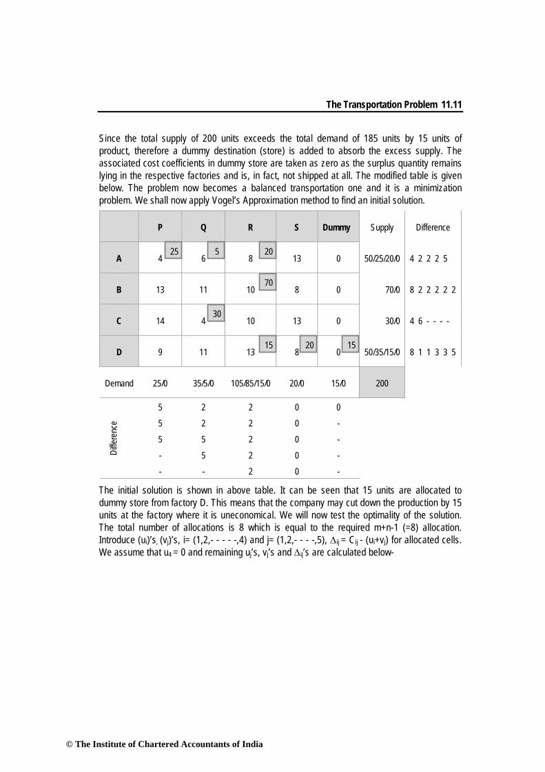
Since the total supply of 200 units exceeds the total demand of 185 units by 15 units of product, therefore a dummy destination (store) is added to absorb the excess supply. The associated cost coefficients in dummy store are taken as zero as the surplus quantity remains lying in the respective factories and is, in fact, not shipped at all. The modified table is given below. The problem now becomes a balanced transportation one and it is a minimization problem. We shall now apply Vogel’s Approximation method to find an initial solution.
P Q R S Dummy Supply Difference
A 4 6 8 13 0 50/25/20/0 4 2 2 2 5
B 13 11 10 8 0 70/0 8 2 2 2 2 2
C 14 4 10 13 0 30/0 4 6 - - - -
D 9 11 13 8 0 50/35/15/0 8 1 1 3 3 5
Demand 25/0 35/5/0 105/85/15/0 20/0 15/0 200
Diffe
renc
e
5 2 2 0 0
5 2 2 0 -
5 5 2 0 -
- 5 2 0 -
- - 2 0 -
The initial solution is shown in above table. It can be seen that 15 units are allocated to dummy store from factory D. This means that the company may cut down the production by 15 units at the factory where it is uneconomical. We will now test the optimality of the solution. The total number of allocations is 8 which is equal to the required m+n-1 (=8) allocation. Introduce (ui)’s, (vj)’s, i= (1,2,- - - - -,4) and j= (1,2,- - - -,5), ∆ij = Cij - (ui+vj) for allocated cells. We assume that u4 = 0 and remaining uj’s, vj’s and ∆ij’s are calculated below-
25 5 20
70
30
15 20 15
© The Institute of Chartered Accountants of India
11.12 Advanced Management Accounting
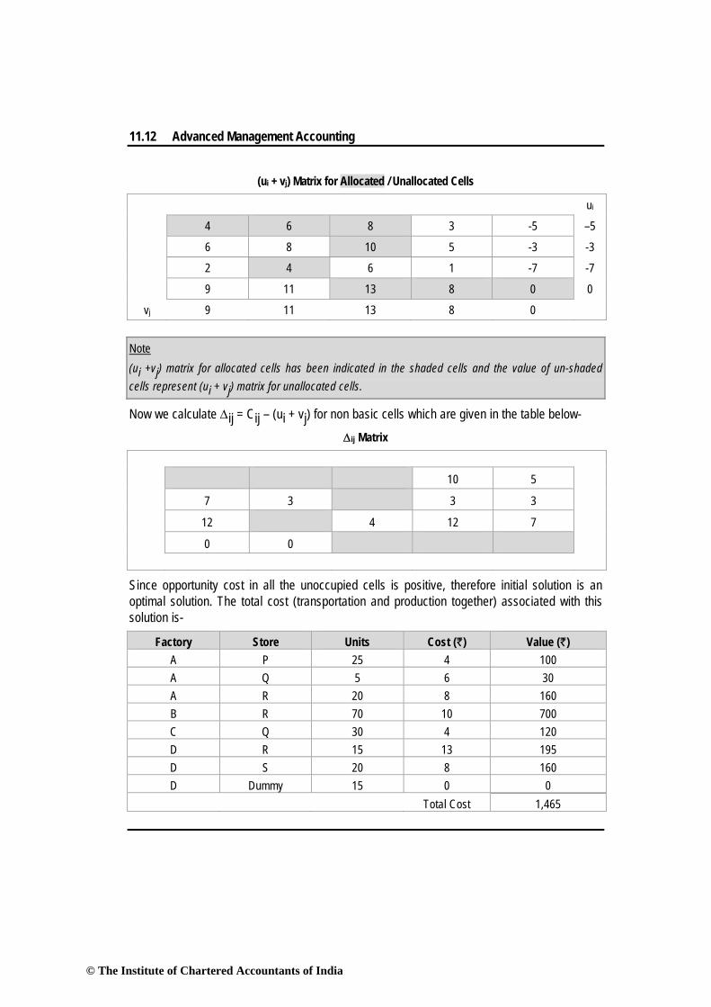
(ui + vj) Matrix for Allocated / Unallocated Cells
ui
4 6 8 3 -5 –5
6 8 10 5 -3 -3
2 4 6 1 -7 -7
9 11 13 8 0 0
vj 9 11 13 8 0 Note (ui +vj) matrix for allocated cells has been indicated in the shaded cells and the value of un-shaded cells represent (ui + vj) matrix for unallocated cells.
Now we calculate Δij = Cij – (ui + vj) for non basic cells which are given in the table below-
Δij Matrix
10 5
7 3 3 3
12 4 12 7
0 0
Since opportunity cost in all the unoccupied cells is positive, therefore initial solution is an optimal solution. The total cost (transportation and production together) associated with this solution is-
Factory Store Units Cost (`) Value (`) A P 25 4 100 A Q 5 6 30 A R 20 8 160 B R 70 10 700 C Q 30 4 120 D R 15 13 195 D S 20 8 160 D Dummy 15 0 0 Total Cost 1,465
© The Institute of Chartered Accountants of India
The Transportation Problem 11.13
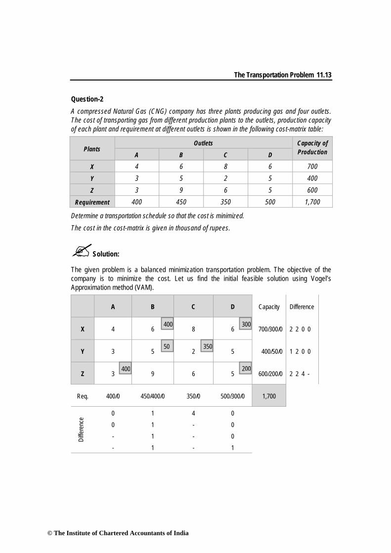
Question-2 A compressed Natural Gas (CNG) company has three plants producing gas and four outlets. The cost of transporting gas from different production plants to the outlets, production capacity of each plant and requirement at different outlets is shown in the following cost-matrix table:
Plants Outlets Capacity of
Production A B C D
X 4 6 8 6 700 Y 3 5 2 5 400 Z 3 9 6 5 600
Requirement 400 450 350 500 1,700
Determine a transportation schedule so that the cost is minimized. The cost in the cost-matrix is given in thousand of rupees.
Solution:
The given problem is a balanced minimization transportation problem. The objective of the company is to minimize the cost. Let us find the initial feasible solution using Vogel’s Approximation method (VAM).
A B C D Capacity Difference
X 4 6 8 6 700/300/0 2 2 0 0
Y 3 5 2 5 400/50/0 1 2 0 0
Z 3 9 6 5 600/200/0 2 2 4 -
Req. 400/0 450/400/0 350/0 500/300/0 1,700
Diffe
renc
e
0 1 4 0
0 1 - 0
- 1 - 0
- 1 - 1
400
300
350
400
50
200
© The Institute of Chartered Accountants of India

11.14 Advanced Management Accounting
The initial feasible solution obtained by VAM is given below-
A B C D Capacity
X 4 6 8 6 700
Y 3 5 2 5 400
Z 3 9 6 5 600
Req. 400 450 350 500 1,700
Since the number of allocations m+n-1 (= 6), let us test the above solution for optimality. Introduce ui (i = 1, 2, 3) and vj (j = 1, 2, 3, 4) such that ∆ij = Cij – (ui + vj) for allocated cells. We assume u1 = 0, and rest of the ui’s, vj’s and ∆ij’s are calculated as below-
(ui + vj) Matrix for Allocated / Unallocated Cells
ui
4 6 3 6 0
3 5 2 5 -1
3 5 2 5 -1
vj 4 6 3 6 Note (ui +vj) matrix for allocated cells has been indicated in the shaded cells and the value of un-shaded cells represent (ui + vj) matrix for unallocated cells.
Now we calculate Δij = Cij – (ui + vj) for non basic cells which are given in the table below-
Δij Matrix
0 5
0 0
4 4
400
300
350
400
50
200
© The Institute of Chartered Accountants of India
The Transportation Problem 11.15
On calculating ∆ij’s for non-allocated cells, we found that all the ∆ij ≥ 0, hence the initial solution obtained above is optimal. The optimal allocations are given below-
Plants Outlet Units Cost (`) Total Cost (`)
X B 400 6 2,400
X D 300 6 1,800
Y B 50 5 250
Y C 350 2 700
Z A 400 3 1,200
Z D 200 5 1,000
Total 7,350
The minimum cost equals to 7,350 thousand rupees. Since some of the ∆ij’s are equal to 0, the above solution is not unique. Alternative solutions exist. Question-3 Consider the following data for the transportation problem:
Factory Destination Supply to be exhausted (1) (2) (3)
A 5 1 7 10
B 6 4 6 80
C 3 2 5 15
Demand 75 20 50
Since there is not enough supply, some of the demands at the three destinations may not be satisfied. For the unsatisfied demands, let the penalty costs be rupees 1, 2 and 3 for destinations (1), (2) and (3) respectively.
Solution:
The initial solution is obtained below by Vogel’s Approximation method (VAM).
© The Institute of Chartered Accountants of India
11.16 Advanced Management Accounting
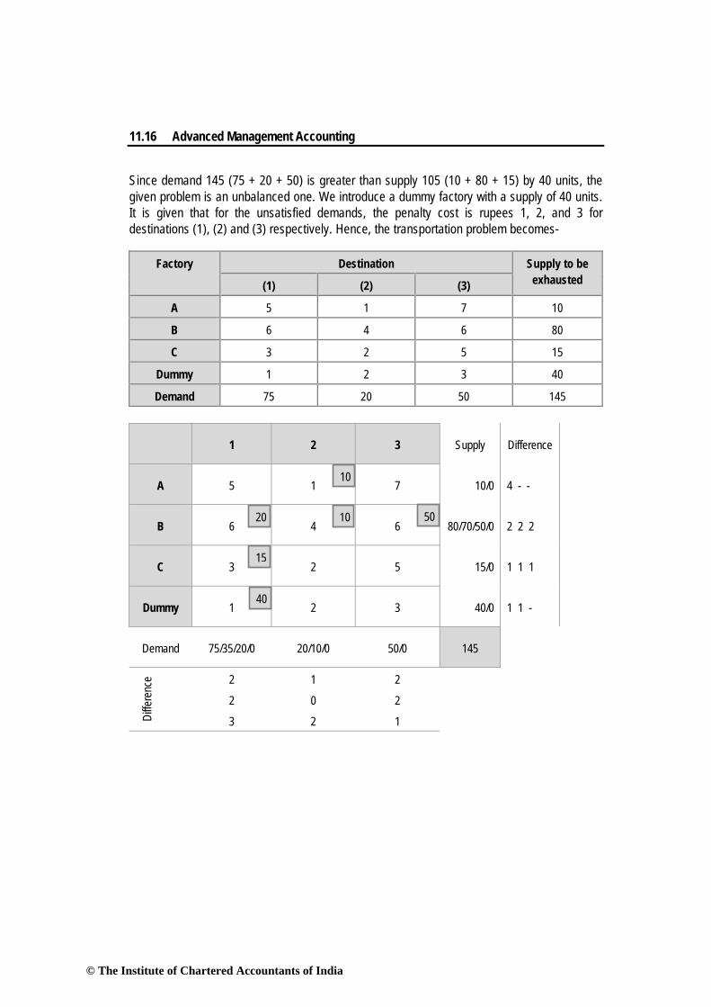
Since demand 145 (75 + 20 + 50) is greater than supply 105 (10 + 80 + 15) by 40 units, the given problem is an unbalanced one. We introduce a dummy factory with a supply of 40 units. It is given that for the unsatisfied demands, the penalty cost is rupees 1, 2, and 3 for destinations (1), (2) and (3) respectively. Hence, the transportation problem becomes-
Factory Destination Supply to be exhausted (1) (2) (3)
A 5 1 7 10
B 6 4 6 80
C 3 2 5 15
Dummy 1 2 3 40
Demand 75 20 50 145
1 2 3 Supply Difference
A 5 1 7 10/0 4 - -
B 6 4 6 80/70/50/0 2 2 2
C 3 2 5 15/0 1 1 1
Dummy 1 2 3 40/0 1 1 -
Demand 75/35/20/0 20/10/0 50/0 145
Diffe
renc
e 2 1 2
2 0 2
3 2 1
20
15
10
10
40
50
© The Institute of Chartered Accountants of India
The Transportation Problem 11.17
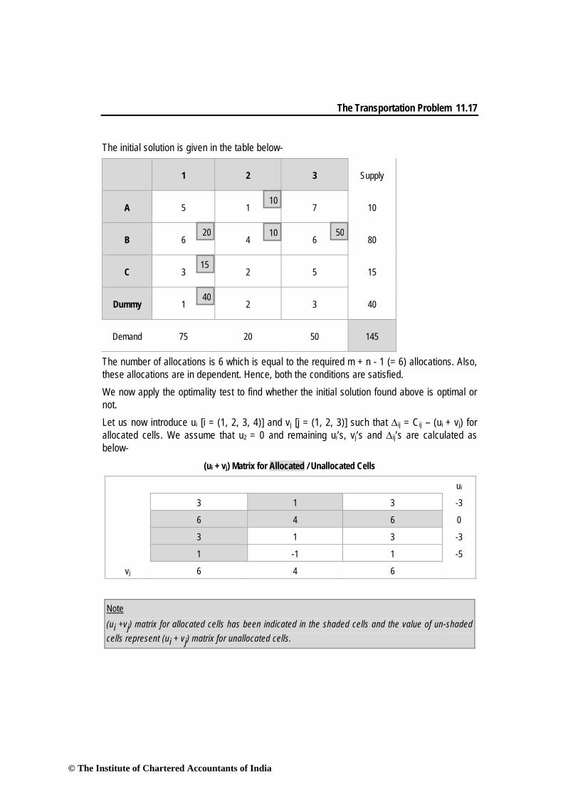
The initial solution is given in the table below-
1 2 3 Supply
A 5 1 7 10
B 6 4 6 80
C 3 2 5 15
Dummy 1 2 3 40
Demand 75 20 50 145
The number of allocations is 6 which is equal to the required m + n - 1 (= 6) allocations. Also, these allocations are in dependent. Hence, both the conditions are satisfied. We now apply the optimality test to find whether the initial solution found above is optimal or not. Let us now introduce ui [i = (1, 2, 3, 4)] and vj [j = (1, 2, 3)] such that ∆ij = Cij – (ui + vj) for allocated cells. We assume that u2 = 0 and remaining ui’s, vj’s and ∆ij’s are calculated as below-
(ui + vj) Matrix for Allocated / Unallocated Cells
ui
3 1 3 -3
6 4 6 0
3 1 3 -3
1 -1 1 -5
vj 6 4 6
Note (ui +vj) matrix for allocated cells has been indicated in the shaded cells and the value of un-shaded cells represent (ui + vj) matrix for unallocated cells.
20
15
10
10
40
50
© The Institute of Chartered Accountants of India

11.18 Advanced Management Accounting
Now we calculate Δij = Cij – (ui + vj) for non basic cells which are given in the table below-
Δij Matrix
2 4
1 2
3 2
Since all ∆ij’s for non basic cells are positive, therefore, the solution obtained above is an optimal one. The allocation of factories to destinations and their cost is given below-
Factory Destination Units Cost (`) Total Cost (`) Type
A (2) 10 1 10
Transportation Cost
B (1) 20 6 120
B (2) 10 4 40
B (3) 50 6 300
C (1) 15 3 45
Dummy (1) 40 1 40 Penalty Cost
Total 555 Question-4 The initial allocation of a transportation problem, alongwith the unit cost of transportation from each origin to destination is given below. You are required to arrive at the minimum transportation cost by the Vogel’s Approximation method and check for optimality.
© The Institute of Chartered Accountants of India
The Transportation Problem 11.19
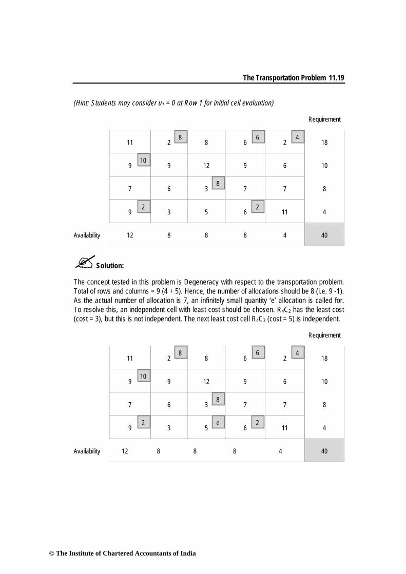
(Hint: Students may consider u1 = 0 at Row 1 for initial cell evaluation)
Requirement
11 2 8 6 2 18
9 9 12 9 6 10
7 6 3 7 7 8
9 3 5 6 11 4
Availability 12 8 8 8 4 40
Solution:
The concept tested in this problem is Degeneracy with respect to the transportation problem. Total of rows and columns = 9 (4 + 5). Hence, the number of allocations should be 8 (i.e. 9 -1). As the actual number of allocation is 7, an infinitely small quantity ‘e’ allocation is called for. To resolve this, an independent cell with least cost should be chosen. R4C2 has the least cost (cost = 3), but this is not independent. The next least cost cell R4C3 (cost = 5) is independent.
Requirement
11 2 8 6 2 18
9 9 12 9 6 10
7 6 3 7 7 8
9 3 5 6 11 4
Availability 12 8 8 8 4 40
10
8
8
2 2
4 6
10
8
8
2 2
4 6
e
© The Institute of Chartered Accountants of India
11.20 Advanced Management Accounting
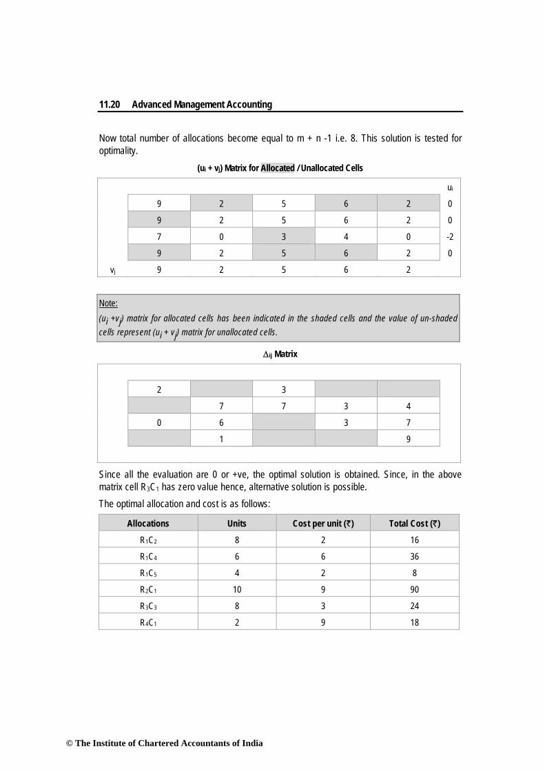
Now total number of allocations become equal to m + n -1 i.e. 8. This solution is tested for optimality.
(ui + vj) Matrix for Allocated / Unallocated Cells
ui
9 2 5 6 2 0
9 2 5 6 2 0
7 0 3 4 0 -2
9 2 5 6 2 0
vj 9 2 5 6 2
Note: (ui +vj) matrix for allocated cells has been indicated in the shaded cells and the value of un-shaded cells represent (ui + vj) matrix for unallocated cells.
Δij Matrix
2 3
7 7 3 4
0 6 3 7
1 9
Since all the evaluation are 0 or +ve, the optimal solution is obtained. Since, in the above matrix cell R3C1 has zero value hence, alternative solution is possible. The optimal allocation and cost is as follows:
Allocations Units Cost per unit (`) Total Cost (`)
R1C2 8 2 16
R1C4 6 6 36
R1C5 4 2 8
R2C1 10 9 90
R3C3 8 3 24
R4C1 2 9 18
© The Institute of Chartered Accountants of India
The Transportation Problem 11.21
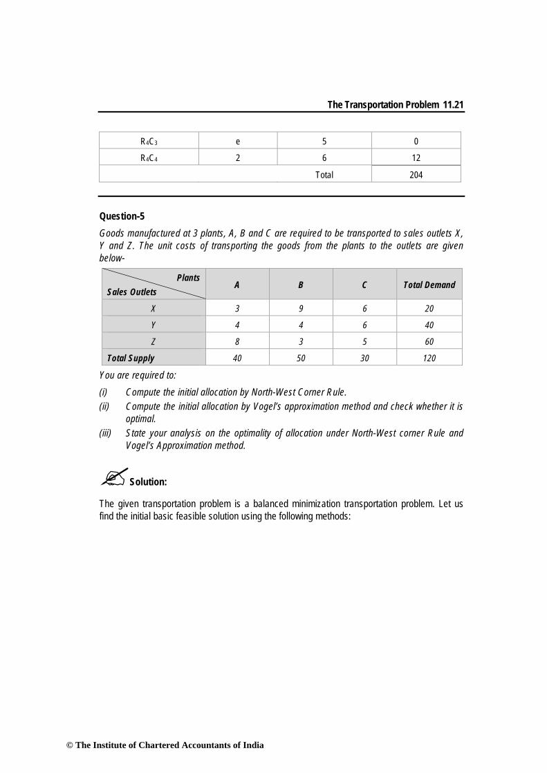
R4C3 e 5 0
R4C4 2 6 12
Total 204 Question-5 Goods manufactured at 3 plants, A, B and C are required to be transported to sales outlets X, Y and Z. The unit costs of transporting the goods from the plants to the outlets are given below-
Plants Sales Outlets
A B C Total Demand
X 3 9 6 20
Y 4 4 6 40
Z 8 3 5 60
Total Supply 40 50 30 120
You are required to: (i) Compute the initial allocation by North-West Corner Rule. (ii) Compute the initial allocation by Vogel’s approximation method and check whether it is
optimal. (iii) State your analysis on the optimality of allocation under North-West corner Rule and
Vogel’s Approximation method.
Solution:
The given transportation problem is a balanced minimization transportation problem. Let us find the initial basic feasible solution using the following methods:
© The Institute of Chartered Accountants of India
11.22 Advanced Management Accounting
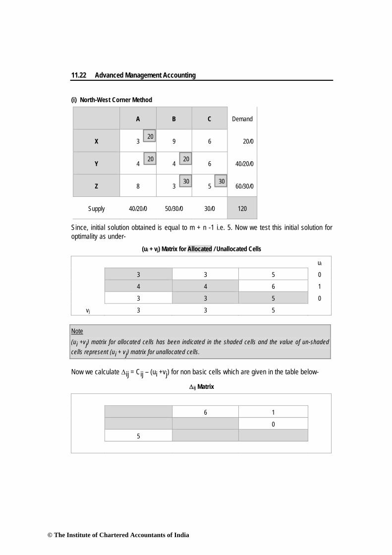
(i) North-West Corner Method
A B C Demand
X 3 9 6 20/0
Y 4 4 6 40/20/0
Z 8 3 5 60/30/0
Supply 40/20/0 50/30/0 30/0 120
Since, initial solution obtained is equal to m + n -1 i.e. 5. Now we test this initial solution for optimality as under-
(ui + vj) Matrix for Allocated / Unallocated Cells
ui
3 3 5 0
4 4 6 1
3 3 5 0
vj 3 3 5 Note (ui +vj) matrix for allocated cells has been indicated in the shaded cells and the value of un-shaded cells represent (ui + vj) matrix for unallocated cells.
Now we calculate Δij = Cij – (ui +vj) for non basic cells which are given in the table below-
Δij Matrix
6 1
0
5
20
20
30
20
30
© The Institute of Chartered Accountants of India
The Transportation Problem 11.23
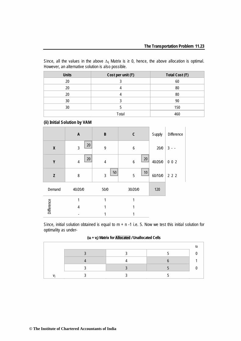
Since, all the values in the above Δij Matrix is ≥ 0, hence, the above allocation is optimal. However, an alternative solution is also possible.
Units Cost per unit (`) Total Cost (`) 20 3 60 20 4 80 20 4 80 30 3 90 30 5 150
Total 460
(ii) Initial Solution by VAM
A B C Supply Difference
X 3 9 6 20/0 3 - -
Y 4 4 6 40/20/0 0 0 2
Z 8 3 5 60/10/0 2 2 2
Demand 40/20/0 50/0 30/20/0 120
Diffe
renc
e 1 1 1
4 1 1
- 1 1
Since, initial solution obtained is equal to m + n -1 i.e. 5. Now we test this initial solution for optimality as under-
(ui + vj) Matrix for Allocated / Unallocated Cells
ui
3 3 5 0
4 4 6 1
3 3 5 0
vj 3 3 5
20
20
50 10
20
© The Institute of Chartered Accountants of India
11.24 Advanced Management Accounting
Note (ui +vj) matrix for allocated cells has been indicated in the shaded cells and the value of un-shaded cells represent (ui + vj) matrix for unallocated cells.
Now we calculate Δij = Cij – (ui +vj) for non basic cells which are given in the table below-
Δij Matrix
6 1
0
5
Since, all the values in the above Δij Matrix is ≥ 0, hence, the above allocation is optimal. However, an alternative solution is also possible.
Units Cost per unit (`) Total Cost (`)
20 3 60
20 4 80
50 3 150
20 6 120
10 5 50
Total 460
(iii)
The both solutions obtained from North-West Corner method and Vogel’s Approximation method is optimal. Under North-West Corner method the allocation at cell R2C3 can alternatively allocated to cell R2C2. Under VAM method also the allocation at cell R2C2 can be allocated to cell R2C3. The both method has the same optimal solution and total cost. Question-6 The cost per unit of transporting goods from the factories X, Y, Z to destinations. A, B and C, and the quantities demanded and supplied are tabulated below. As the company is working out the optimum logistics, the Govt.; has announced a fall in oil prices. The revised unit costs
© The Institute of Chartered Accountants of India
The Transportation Problem 11.25
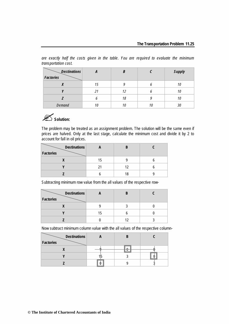
are exactly half the costs given in the table. You are required to evaluate the minimum transportation cost.
Destinations Factories
A B C Supply
X 15 9 6 10
Y 21 12 6 10
Z 6 18 9 10
Demand 10 10 10 30
Solution:
The problem may be treated as an assignment problem. The solution will be the same even if prices are halved. Only at the last stage, calculate the minimum cost and divide it by 2 to account for fall in oil prices.
Destinations Factories
A B C
X 15 9 6
Y 21 12 6
Z 6 18 9
Subtracting minimum row value from the all values of the respective row-
Destinations Factories
A B C
X 9 3 0
Y 15 6 0
Z 0 12 3
Now subtract minimum column value with the all values of the respective column-
Destinations Factories
A B C
X 9 0 0
Y 15 3 0
Z 0 9 3
© The Institute of Chartered Accountants of India
11.26 Advanced Management Accounting
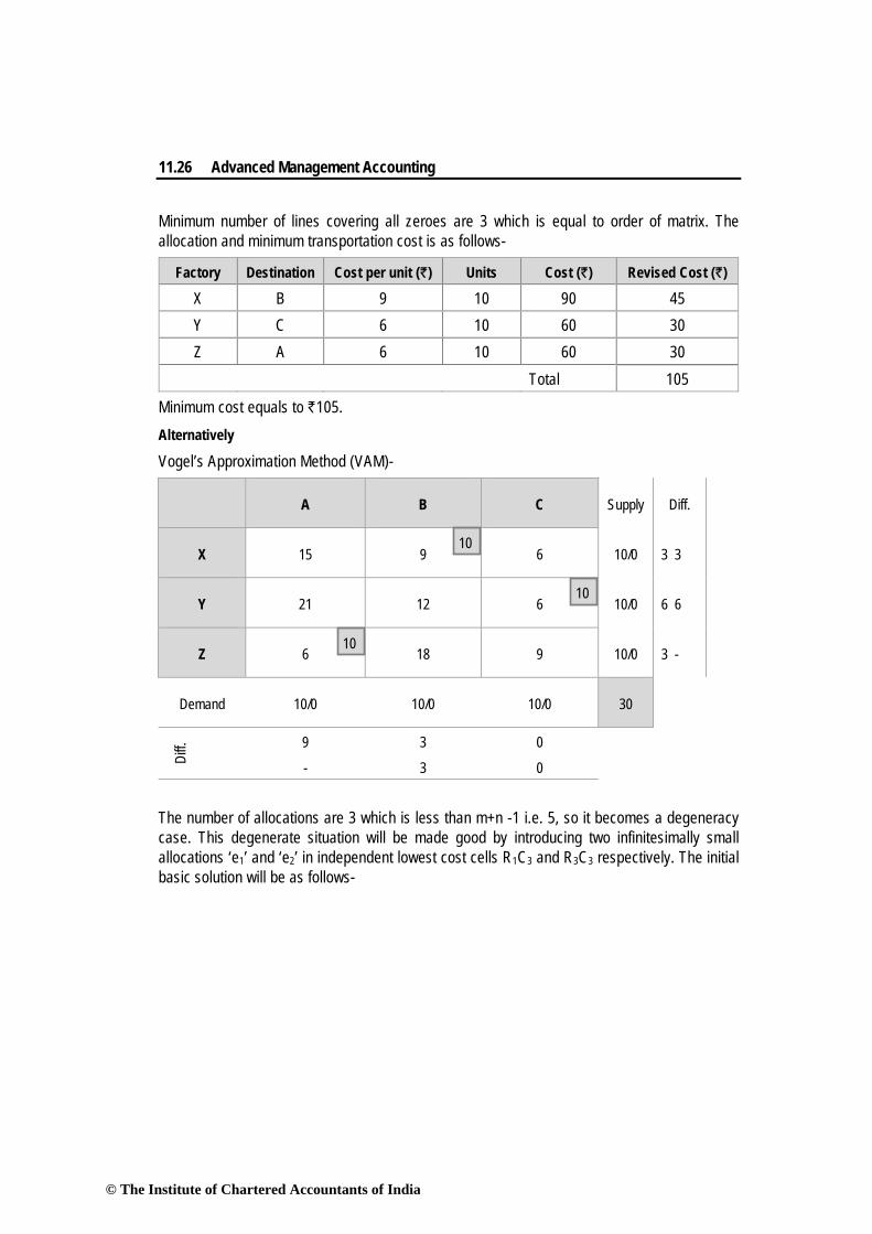
Minimum number of lines covering all zeroes are 3 which is equal to order of matrix. The allocation and minimum transportation cost is as follows-
Factory Destination Cost per unit (`) Units Cost (`) Revised Cost (`)
X B 9 10 90 45 Y C 6 10 60 30 Z A 6 10 60 30
Total 105 Minimum cost equals to `105. Alternatively
Vogel’s Approximation Method (VAM)-
A B C Supply Diff.
X 15 9 6 10/0 3 3
Y 21 12 6 10/0 6 6
Z 6 18 9 10/0 3 -
Demand 10/0 10/0 10/0 30
Diff. 9 3 0
- 3 0
The number of allocations are 3 which is less than m+n -1 i.e. 5, so it becomes a degeneracy case. This degenerate situation will be made good by introducing two infinitesimally small allocations ‘e1’ and ‘e2’ in independent lowest cost cells R1C3 and R3C3 respectively. The initial basic solution will be as follows-
10
10
10
© The Institute of Chartered Accountants of India
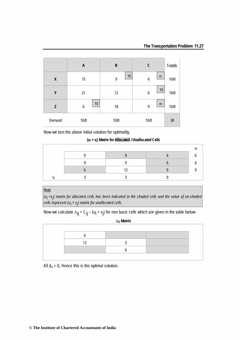
The Transportation Problem 11.27
A B C Supply
X 15 9 6 10/0
Y 21 12 6 10/0
Z 6 18 9 10/0
Demand 10/0 10/0 10/0 30
Now we test the above initial solution for optimality. (ui + vj) Matrix for Allocated / Unallocated Cells
ui
9 9 6 6
9 9 6 6
6 12 9 9
vj 3 3 0
Note (ui +vj) matrix for allocated cells has been indicated in the shaded cells and the value of un-shaded cells represent (ui + vj) matrix for unallocated cells.
Now we calculate Δij = Cij – (ui + vj) for non basic cells which are given in the table below-
Δij Matrix
6
12 3
6
All Δij > 0, Hence this is the optimal solution.
10
10
10
e1
e2
© The Institute of Chartered Accountants of India
11.28 Advanced Management Accounting
Factory Destination Cost per unit (`) Units Cost (`) Revised Cost (`)
X B 9 10 90 45 X C 6 e1 0 0 Y C 6 10 60 30 Z A 6 10 60 30 Z C 9 e2 0 0
Total 105 Total minimum transportation cost is ` 105. Question-7 The following matrix is a minimization problem for transportation cost. The unit transportation costs are given at the right hand corners of the cells and the ijΔ values are encircled.
D1 D2 D3 Supply
F1 500
F2 300 300
F3 200 200
Demand 300 400 300 1,000
Find the optimum solution (s) and the minimum cost.
Solution:
As we know Δij values are given for unallocated cells. Hence, the remaining cells represent the allocated cells which is 5 and equal to m + n -1 (no. of columns + no of rows – 1). Now we fill up the allocated cells with allocated units.
9
6
6
5
8
3
4
4 4
7
0 8
8
© The Institute of Chartered Accountants of India
The Transportation Problem 11.29
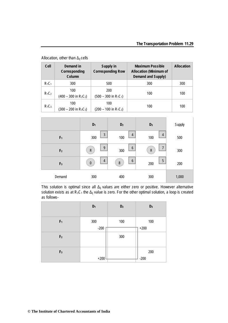
Allocation, other than Δij cells
Cell Demand in Corresponding
Column
Supply in Corresponding Row
Maximum Possible Allocation (Minimum of
Demand and Supply)
Allocation
R1C1 300 500 300 300
R1C2 100
(400 – 300 in R2C2) 200
(500 – 300 in R1C1) 100 100
R1C3 100
(300 – 200 in R3C3) 100
(200 – 100 in R1C2) 100 100
D1 D2 D3 Supply
F1 300 100 100 500
F2 300 300
F3 200 200
Demand 300 400 300 1,000
This solution is optimal since all Δij values are either zero or positive. However alternative solution exists as at R3C1 the Δij value is zero. For the other optimal solution, a loop is created as follows-
D1
D2
D3
F1 300
-200
100 100
+200
F2 300
F3
+200
200
-200
9
6
6
5
8
3
4
4 4
7
0 8
8
© The Institute of Chartered Accountants of India
11.30 Advanced Management Accounting
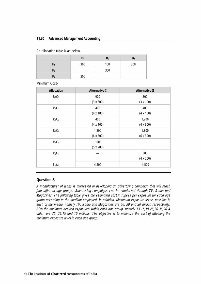
Re-allocation table is as below-
D1 D2 D3
F1 100 100 300
F2 300
F3 200
Minimum Cost-
Allocation Alternative-I Alternative-II
R1C1 900 (3 x 300)
300 (3 x 100)
R1C2 400 (4 x 100)
400 (4 x 100)
R1C3 400 (4 x 100)
1,200 (4 x 300)
R2C2 1,800 (6 x 300)
1,800 (6 x 300)
R3C3 1,000 (5 x 200)
---
R3C1 --- 800 (4 x 200)
Total 4,500 4,500 Question-8 A manufacturer of jeans is interested in developing an advertising campaign that will reach four different age groups. Advertising campaigns can be conducted through TV, Radio and Magazines. The following table gives the estimated cost in rupees per exposure for each age group according to the medium employed. In addition, Maximum exposure levels possible in each of the media, namely TV, Radio and Magazines are 40, 30 and 20 million respectively. Also the minimum desired exposures within each age group, namely 13-18,19-25,26-35,36 & older, are 30, 25,15 and 10 millions. The objective is to minimize the cost of attaining the minimum exposure level in each age group.
© The Institute of Chartered Accountants of India
The Transportation Problem 11.31
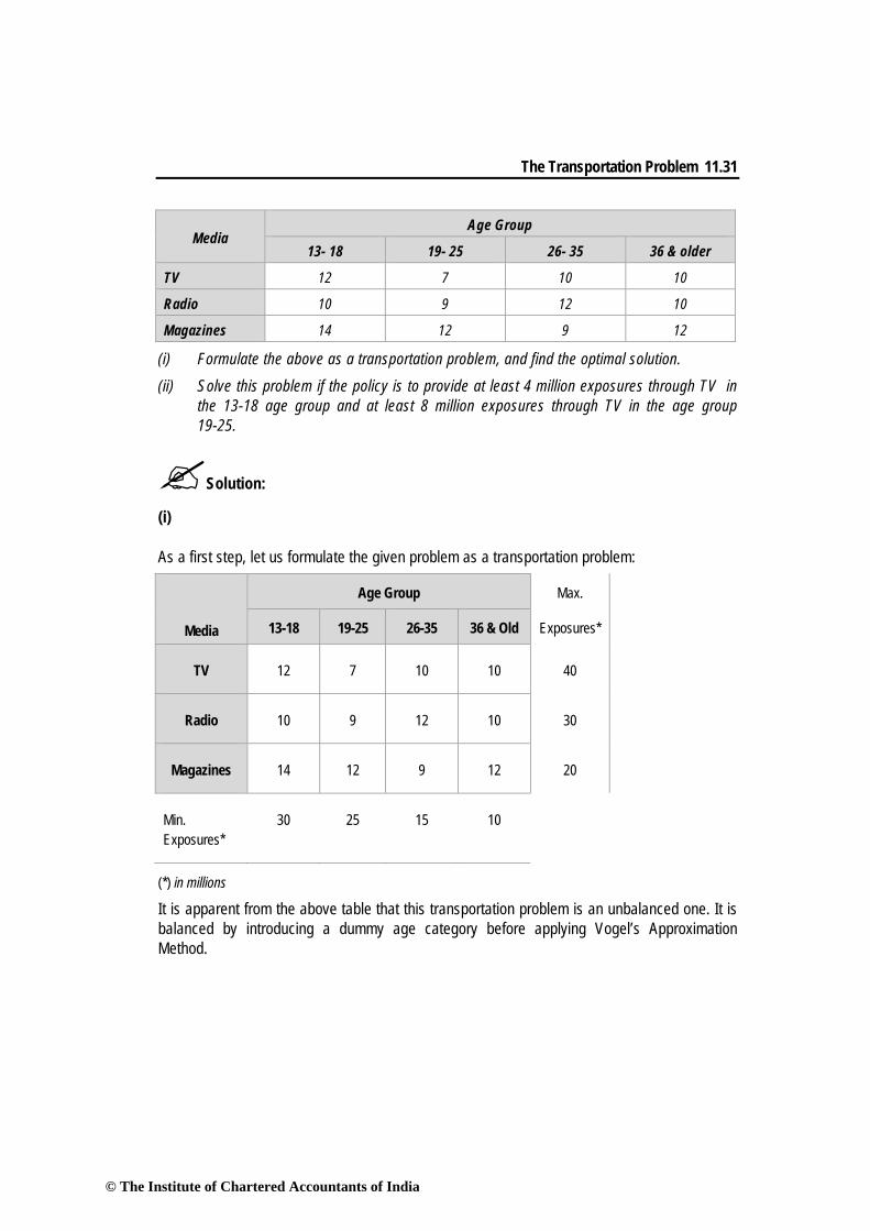
Media Age Group
13- 18 19- 25 26- 35 36 & older
TV 12 7 10 10
Radio 10 9 12 10
Magazines 14 12 9 12
(i) Formulate the above as a transportation problem, and find the optimal solution. (ii) Solve this problem if the policy is to provide at least 4 million exposures through TV in
the 13-18 age group and at least 8 million exposures through TV in the age group 19-25.
Solution:
(i) As a first step, let us formulate the given problem as a transportation problem:
(*) in millions It is apparent from the above table that this transportation problem is an unbalanced one. It is balanced by introducing a dummy age category before applying Vogel’s Approximation Method.
Media
Age Group Max.
13-18 19-25 26-35 36 & Old Exposures*
TV 12 7 10 10 40
Radio 10 9 12 10 30
Magazines 14 12 9 12 20
Min. Exposures*
30 25 15 10
© The Institute of Chartered Accountants of India
11.32 Advanced Management Accounting
Media
Age Group Max. Exposures
Difference
13-18 19-25 26-35 36 & Old Dummy
TV 12 7 10 10 0 40/15/10/0 7 3 0 0 0
Radio 10 9 12 10 0 30/0 9 1 0 0 -
Mag. 14 12 9 12 0 20/10/0 9 3 3 - -
Min. Exposure 30/0 25/0 15/5/0 10/0 10/0 90
Diffe
renc
e
2 2 1 0 0
2 2 1 0 -
2 - 1 0 -
2 - 2 0 -
- - 10 10 -
The solution given by VAM is degenerate since there are only six assignments. Let us put an ‘e’ in the least cost independent cell to check for optimality.
Media
Age Group Max. Exposures 13-18 19-25 26-35 36 & Old Dummy
TV 12 7 10 10 0 40/15/10/0
Radio 10 9 12 10 0 30/0
Mag. 14 12 9 12 0 20/10/0
Min. Exposure 30/0 25/0 15/5/0 10/0 10/0 90
30
25 5
10
10
10
25 5 10
30
10 10
e
© The Institute of Chartered Accountants of India
The Transportation Problem 11.33
(ui + vj) Matrix for Allocated / Unallocated Cells
ui
11 7 10 10 1 0
10 6 9 9 0 -1
10 6 9 9 0 -1
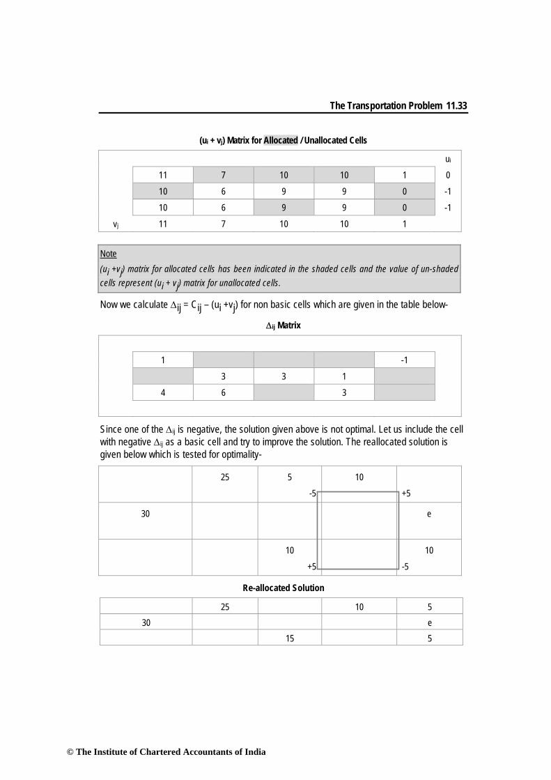
vj 11 7 10 10 1 Note (ui +vj) matrix for allocated cells has been indicated in the shaded cells and the value of un-shaded cells represent (ui + vj) matrix for unallocated cells.
Now we calculate Δij = Cij – (ui +vj) for non basic cells which are given in the table below-
Δij Matrix
1 -1
3 3 1
4 6 3
Since one of the Δij is negative, the solution given above is not optimal. Let us include the cell with negative Δij as a basic cell and try to improve the solution. The reallocated solution is given below which is tested for optimality-
25
5
-5
10
+5
30
e
10
+5
10
-5
Re-allocated Solution
25 10 5 30 e
15 5
© The Institute of Chartered Accountants of India
11.34 Advanced Management Accounting
(ui + vj) Matrix for Allocated / Unallocated Cells
ui
10 7 9 10 0 0
10 7 9 10 0 0
10 7 9 10 0 0
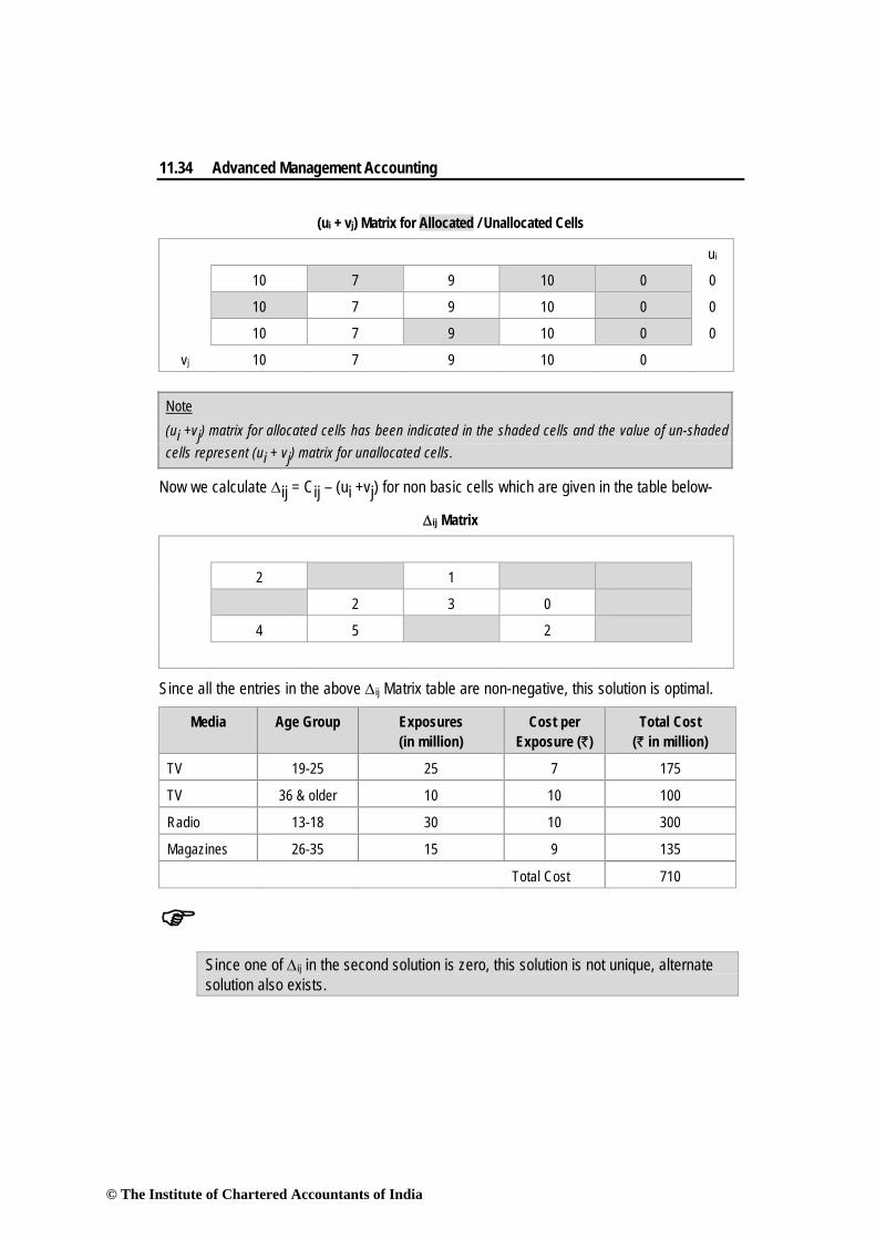
vj 10 7 9 10 0 Note (ui +vj) matrix for allocated cells has been indicated in the shaded cells and the value of un-shaded cells represent (ui + vj) matrix for unallocated cells.
Now we calculate Δij = Cij – (ui +vj) for non basic cells which are given in the table below-
Δij Matrix
2 1
2 3 0
4 5 2
Since all the entries in the above Δij Matrix table are non-negative, this solution is optimal.
Media Age Group Exposures (in million)
Cost per Exposure (`)
Total Cost (` in million)
TV 19-25 25 7 175
TV 36 & older 10 10 100
Radio 13-18 30 10 300
Magazines 26-35 15 9 135
Total Cost 710
Since one of Δij in the second solution is zero, this solution is not unique, alternate solution also exists.
© The Institute of Chartered Accountants of India
The Transportation Problem 11.35
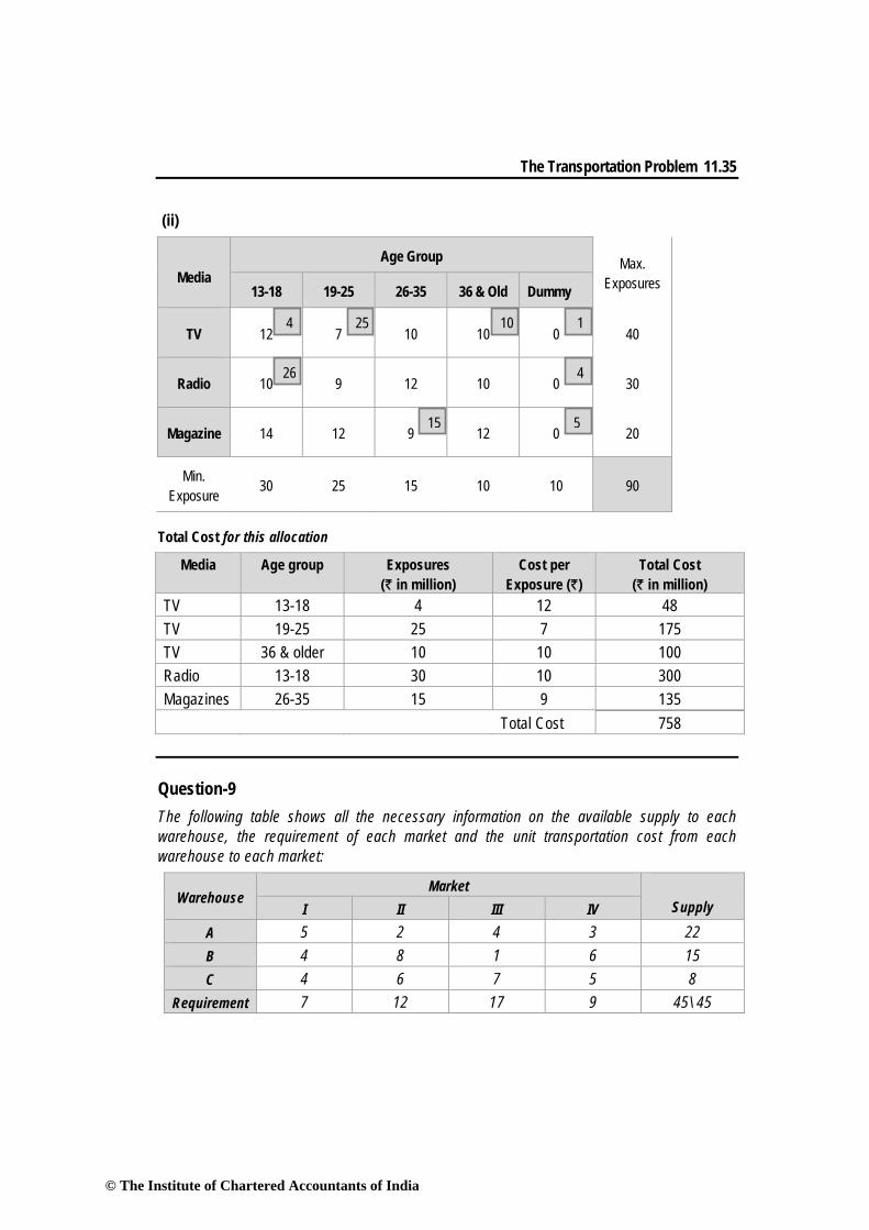
(ii)
Total Cost for this allocation
Media Age group Exposures (` in million)
Cost per Exposure (`)
Total Cost (` in million)
TV 13-18 4 12 48 TV 19-25 25 7 175 TV 36 & older 10 10 100 Radio 13-18 30 10 300 Magazines 26-35 15 9 135 Total Cost 758
Question-9 The following table shows all the necessary information on the available supply to each warehouse, the requirement of each market and the unit transportation cost from each warehouse to each market:
Warehouse Market
Supply I II III IV A 5 2 4 3 22 B 4 8 1 6 15 C 4 6 7 5 8
Requirement 7 12 17 9 45\ 45
Media
Age Group Max. Exposures 13-18 19-25 26-35 36 & Old Dummy
TV 12 7 10 10 0 40
Radio 10 9 12 10 0 30
Magazine 14 12 9 12 0 20
Min. Exposure 30 25 15 10 10 90
25 4 10
26
15 5
4
1
© The Institute of Chartered Accountants of India
11.36 Advanced Management Accounting
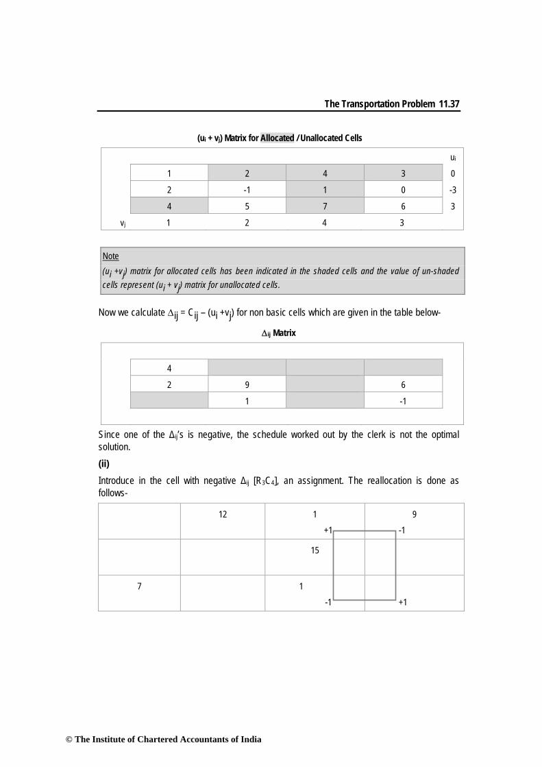
The shipping clerk has worked out the following schedule from his experience: 12 units from A to ll 1 unit from A to lll 9 units from A to lV 15 units from B to lll 7 units from C to l and 1 unit from C to III You are required to answer the following: (i) Check and see if the clerk has the optimal schedule; (ii) Find the optimal schedule and minimum total shipping cost; and (iii) If the clerk is approached by a carrier of route C to ll, Who offers to reduce his rate in
the hope of getting some business, by how much should the rate be reduced before the clerk should consider giving him an order ?
Solution:
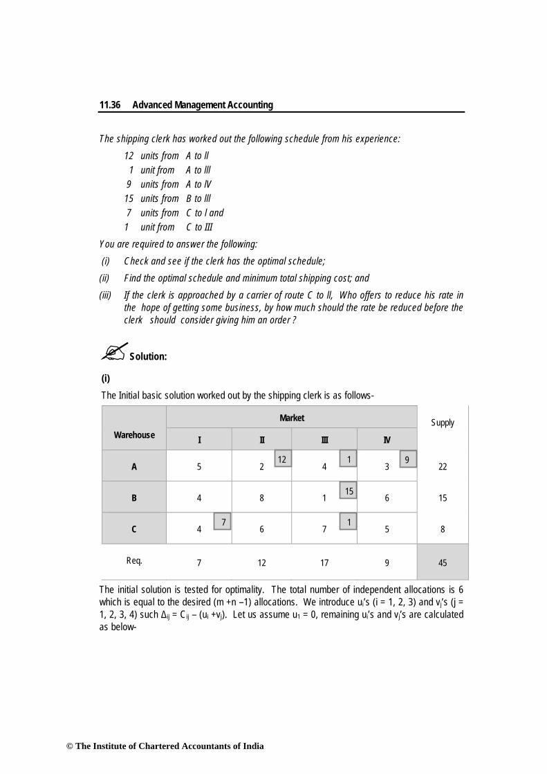
(i) The Initial basic solution worked out by the shipping clerk is as follows-
Warehouse
Market Supply
I II III IV
A 5 2 4 3 22
B 4 8 1 6 15
C 4 6 7 5 8
Req. 7 12 17 9 45
The initial solution is tested for optimality. The total number of independent allocations is 6 which is equal to the desired (m +n –1) allocations. We introduce ui’s (i = 1, 2, 3) and vj’s (j = 1, 2, 3, 4) such Δij = Cij – (ui +vj). Let us assume u1 = 0, remaining ui’s and vj’s are calculated as below-
7
9
15
12 1
1
© The Institute of Chartered Accountants of India
The Transportation Problem 11.37
(ui + vj) Matrix for Allocated / Unallocated Cells
ui
1 2 4 3 0
2 -1 1 0 -3
4 5 7 6 3
vj 1 2 4 3
Note (ui +vj) matrix for allocated cells has been indicated in the shaded cells and the value of un-shaded cells represent (ui + vj) matrix for unallocated cells.
Now we calculate Δij = Cij – (ui +vj) for non basic cells which are given in the table below-
Δij Matrix
4
2 9 6
1 -1
Since one of the Δij’s is negative, the schedule worked out by the clerk is not the optimal solution. (ii) Introduce in the cell with negative Δij [R3C4], an assignment. The reallocation is done as follows-
12
1
+1
9
-1
15
7
1
-1
+1
© The Institute of Chartered Accountants of India
11.38 Advanced Management Accounting
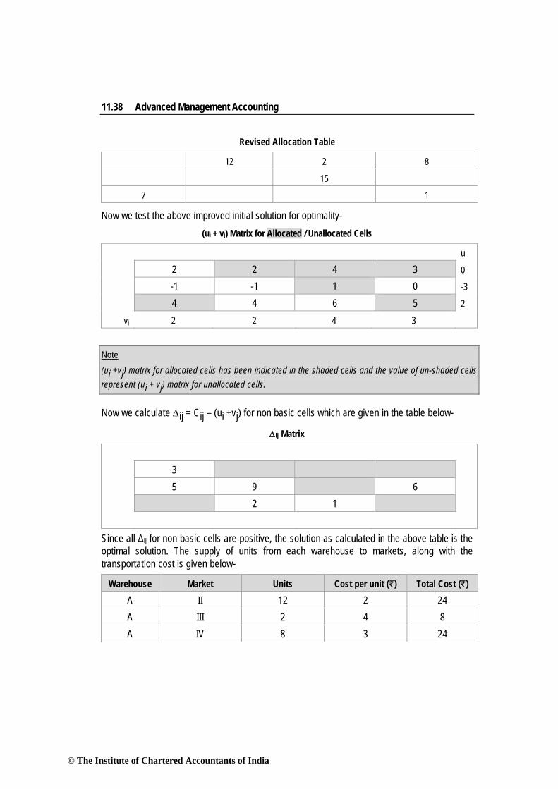
Revised Allocation Table
12 2 8
15
7 1
Now we test the above improved initial solution for optimality- (ui + vj) Matrix for Allocated / Unallocated Cells
ui
2 2 4 3 0
-1 -1 1 0 -3
4 4 6 5 2
vj 2 2 4 3
Note (ui +vj) matrix for allocated cells has been indicated in the shaded cells and the value of un-shaded cells represent (ui + vj) matrix for unallocated cells.
Now we calculate Δij = Cij – (ui +vj) for non basic cells which are given in the table below-
Δij Matrix
3
5 9 6
2 1
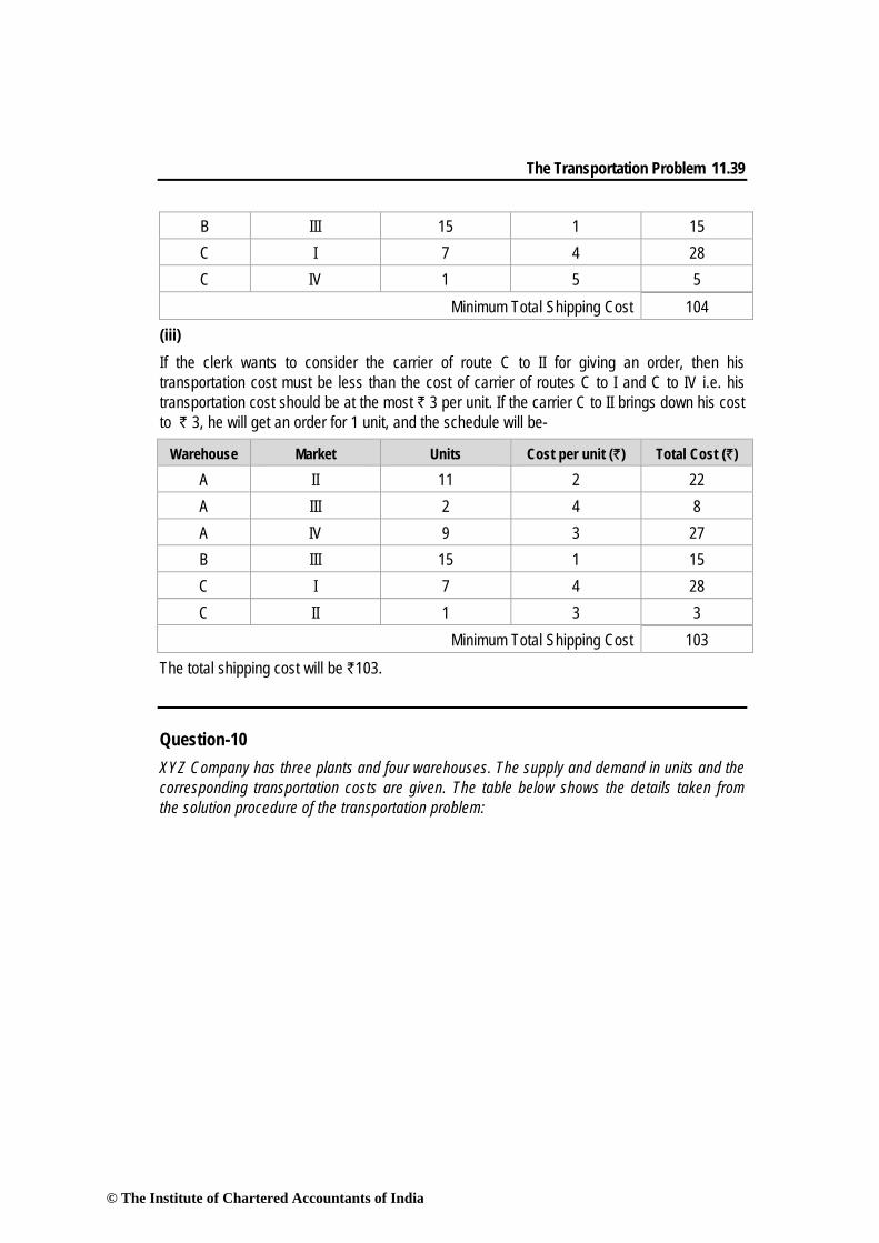
Since all Δij for non basic cells are positive, the solution as calculated in the above table is the optimal solution. The supply of units from each warehouse to markets, along with the transportation cost is given below-
Warehouse Market Units Cost per unit (`) Total Cost (`)
A II 12 2 24 A III 2 4 8 A IV 8 3 24
© The Institute of Chartered Accountants of India
The Transportation Problem 11.39
B III 15 1 15 C I 7 4 28 C IV 1 5 5
Minimum Total Shipping Cost 104 (iii) If the clerk wants to consider the carrier of route C to II for giving an order, then his transportation cost must be less than the cost of carrier of routes C to I and C to IV i.e. his transportation cost should be at the most ` 3 per unit. If the carrier C to II brings down his cost to ` 3, he will get an order for 1 unit, and the schedule will be-
Warehouse Market Units Cost per unit (`) Total Cost (`)
A II 11 2 22 A III 2 4 8 A IV 9 3 27 B III 15 1 15 C I 7 4 28 C II 1 3 3
Minimum Total Shipping Cost 103 The total shipping cost will be `103. Question-10 XYZ Company has three plants and four warehouses. The supply and demand in units and the corresponding transportation costs are given. The table below shows the details taken from the solution procedure of the transportation problem:
© The Institute of Chartered Accountants of India
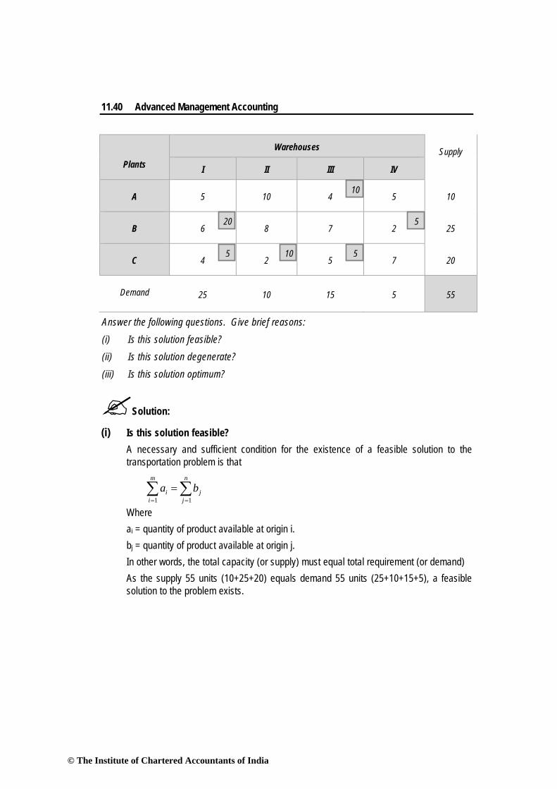
11.40 Advanced Management Accounting
Plants
Warehouses Supply
I II III IV
A 5 10 4 5 10
B 6 8 7 2 25
C 4 2 5 7 20
Demand 25 10 15 5 55
Answer the following questions. Give brief reasons: (i) Is this solution feasible? (ii) Is this solution degenerate? (iii) Is this solution optimum?
Solution:
(i) Is this solution feasible? A necessary and sufficient condition for the existence of a feasible solution to the
transportation problem is that
Where ai = quantity of product available at origin i. bj = quantity of product available at origin j. In other words, the total capacity (or supply) must equal total requirement (or demand) As the supply 55 units (10+25+20) equals demand 55 units (25+10+15+5), a feasible
solution to the problem exists.
∑ ∑= =
=m
i
n
jji ba
1 1
5
5
10
5 10
20
© The Institute of Chartered Accountants of India
The Transportation Problem 11.41
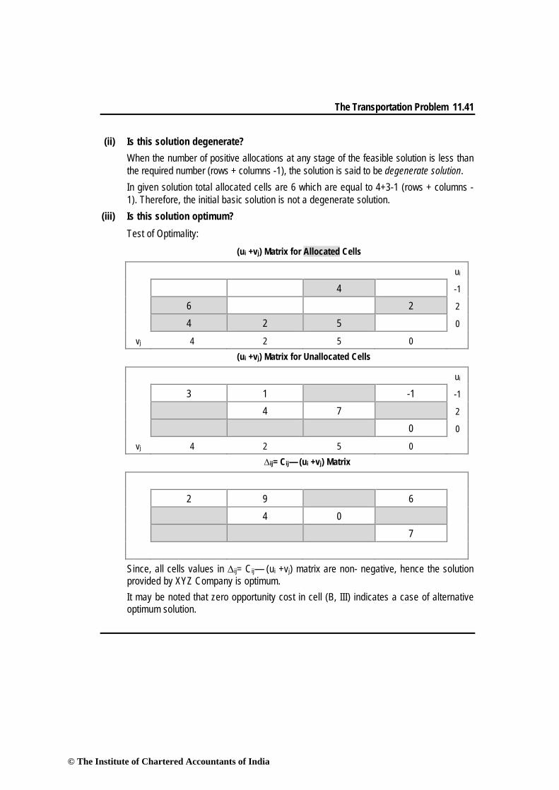
(ii) Is this solution degenerate? When the number of positive allocations at any stage of the feasible solution is less than
the required number (rows + columns -1), the solution is said to be degenerate solution. In given solution total allocated cells are 6 which are equal to 4+3-1 (rows + columns -
1). Therefore, the initial basic solution is not a degenerate solution. (iii) Is this solution optimum? Test of Optimality: (ui +vj) Matrix for Allocated Cells
ui
4 -1
6 2 2
4 2 5 0
vj 4 2 5 0 (ui +vj) Matrix for Unallocated Cells
ui
3 1 -1 -1
4 7 2
0 0
vj 4 2 5 0 ∆ij= Cij— (ui +vj) Matrix
2 9 6
4 0
7
Since, all cells values in ∆ij= Cij— (ui +vj) matrix are non- negative, hence the solution provided by XYZ Company is optimum.
It may be noted that zero opportunity cost in cell (B, III) indicates a case of alternative optimum solution.
© The Institute of Chartered Accountants of India
11.42 Advanced Management Accounting
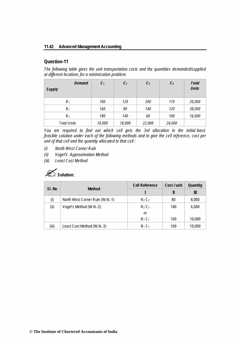
Question-11 The following table gives the unit transportation costs and the quantities demanded/supplied at different locations for a minimization problem:
Demand Supply
C1 C2 C3 C4 Total Units
R1 100 120 200 110 20,000
R2 160 80 140 120 38,000
R3 180 140 60 100 16,000
Total Units 10,000 18,000 22,000 24,000
You are required to find out which cell gets the 3rd allocation in the initial basic feasible solution under each of the following methods and to give the cell reference, cost per unit of that cell and the quantity allocated to that cell : (i) North West Corner Rule (ii) Vogel's Approximation Method (iii) Least Cost Method
Solution:
Sl. No Method Cell Reference Cost / unit Quantity
I II III (i) North West Corner Rule (W.N.-1) R2 C2 80 8,000
(ii) Vogel’s Method (W.N.-2) R2 C3
or R1 C1
140
100
6,000
10,000
(iii) Least Cost Method (W.N.-3) R1 C1 100 10,000
© The Institute of Chartered Accountants of India
The Transportation Problem 11.43
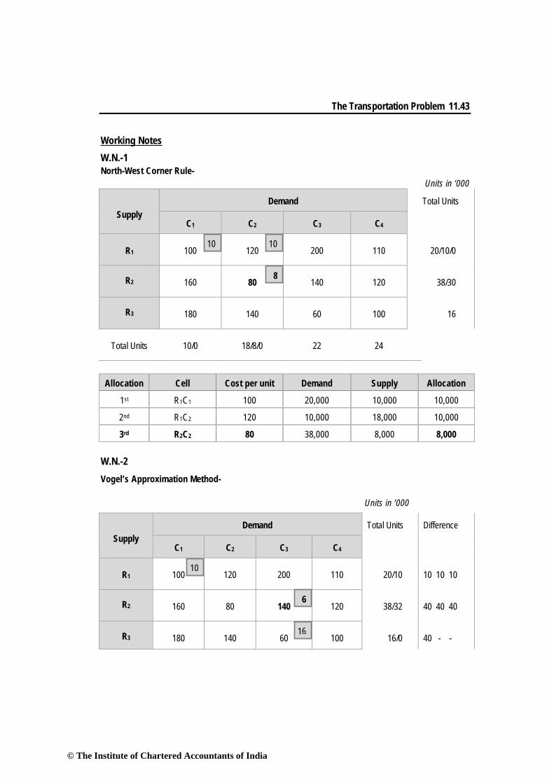
Working Notes W.N.-1 North-West Corner Rule-
Units in ‘000
Supply
Demand Total Units
C1 C2 C3 C4
R1 100 120 200 110 20/10/0
R2 160 80 140 120 38/30
R3 180 140 60 100 16
Total Units 10/0 18/8/0 22 24
Allocation Cell Cost per unit Demand Supply Allocation
1st R1C1 100 20,000 10,000 10,000
2nd R1C2 120 10,000 18,000 10,000
3rd R2C2 80 38,000 8,000 8,000 W.N.-2 Vogel’s Approximation Method-
Units in ‘000
Supply
Demand Total Units Difference
C1 C2 C3 C4
R1 100 120 200 110 20/10 10 10 10
R2 160 80 140 120 38/32 40 40 40
R3 180 140 60 100 16/0 40 - -
10 10
8
6
16
10
© The Institute of Chartered Accountants of India
11.44 Advanced Management Accounting
Total Units 10/0 18 22/6/0 24
Diffe
renc
e 60 40 80 10
60 40 60 10
- 40 60 10
Allocation Cell Cost per unit Demand Supply Allocation
1st R3C3 60 16,000 22,000 16,000
2nd R1C1 100 20,000 10,000 10,000
3rd R2C3 140 38,000 6,000 6,000
Or
Units in ‘000
Supply
Demand Total Units Difference
C1 C2 C3 C4
R1 100 120 200 110 20/10 10 10 10
R2 160 80 140 120 38/32 40 40 40
R3 180 140 60 100 16/0 40 - -
Total Units 10/0 18 22/6/0 24
Diffe
renc
e
60 40 80 10
60 40 60 10
60 40 - 10
6
16
10
© The Institute of Chartered Accountants of India

The Transportation Problem 11.45
Allocation Cell Cost per unit Demand Supply Allocation
1st R3C3 60 16,000 22,000 16,000
2nd R2C3 140 38,000 6,000 6,000
3rd R1C1 100 20,000 10,000 10,000
W.N.-3 Least Cost Method-
Units in ‘000
Supply
Demand Total Units
C1 C2 C3 C4
R1 100 120 200 110 20/10
R2 160 80 140 120 38/20
R3 180 140 60 100 16/0
Total Units 10/0 18/0 22 24
Allocation Cell Cost per unit Demand Supply Allocation
1st R3C3 60 16,000 22,000 16,000
2nd R2C2 80 38,000 18,000 18,000
3rd R1C1 100 20,000 10,000 10,000
10
18
© The Institute of Chartered Accountants of India
11.46 Advanced Management Accounting
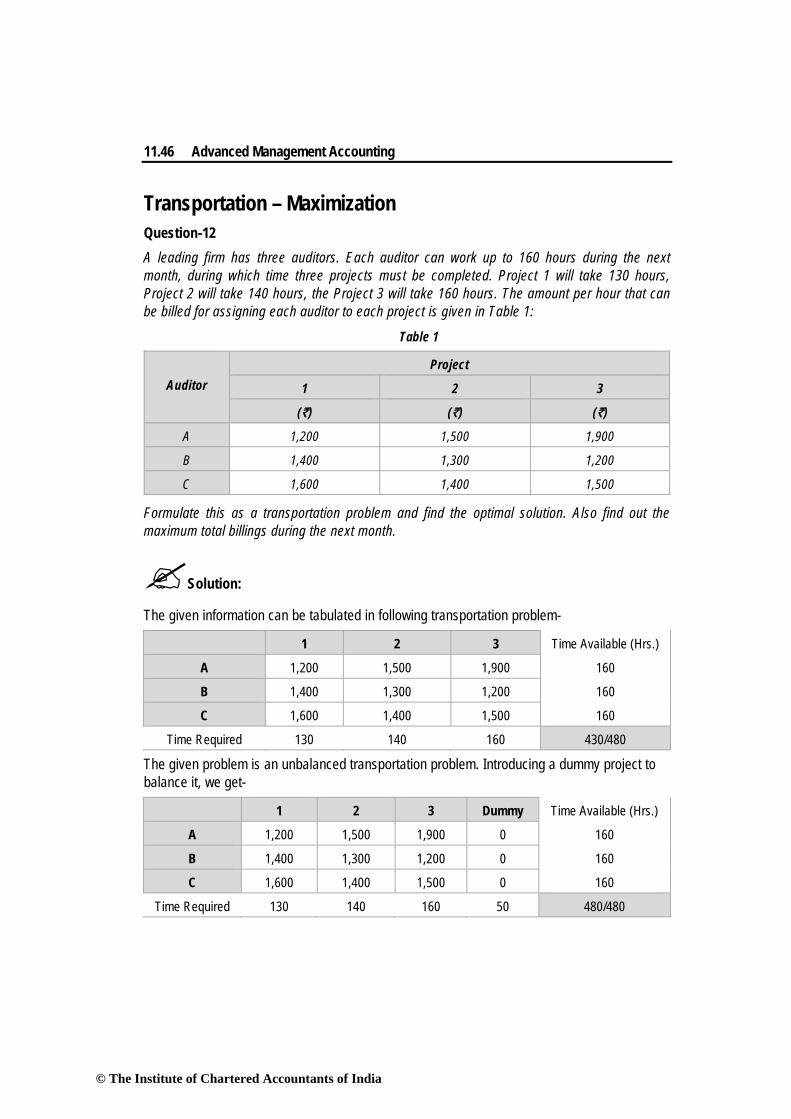
Transportation – Maximization Question-12 A leading firm has three auditors. Each auditor can work up to 160 hours during the next month, during which time three projects must be completed. Project 1 will take 130 hours, Project 2 will take 140 hours, the Project 3 will take 160 hours. The amount per hour that can be billed for assigning each auditor to each project is given in Table 1:
Table 1
Auditor
Project
1 2 3
(`) (`) (`)
A 1,200 1,500 1,900
B 1,400 1,300 1,200
C 1,600 1,400 1,500
Formulate this as a transportation problem and find the optimal solution. Also find out the maximum total billings during the next month.
Solution:
The given information can be tabulated in following transportation problem-
1 2 3 Time Available (Hrs.)
A 1,200 1,500 1,900 160
B 1,400 1,300 1,200 160
C 1,600 1,400 1,500 160
Time Required 130 140 160 430/480
The given problem is an unbalanced transportation problem. Introducing a dummy project to balance it, we get-
1 2 3 Dummy Time Available (Hrs.)
A 1,200 1,500 1,900 0 160
B 1,400 1,300 1,200 0 160
C 1,600 1,400 1,500 0 160
Time Required 130 140 160 50 480/480
© The Institute of Chartered Accountants of India
The Transportation Problem 11.47
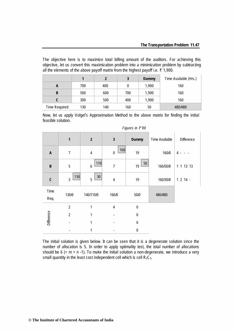
The objective here is to maximize total billing amount of the auditors. For achieving this objective, let us convert this maximization problem into a minimization problem by subtracting all the elements of the above payoff matrix from the highest payoff i.e. ` 1,900.
1 2 3 Dummy Time Available (Hrs.)
A 700 4000 0 1,900 160
B 500 600 700 1,900 160
C 300 500 400 1,900 160
Time Required 130 140 160 50 480/480
Now, let us apply Volgel’s Approximation Method to the above matrix for finding the initial feasible solution. Figures in ` ’00
1 2 3 Dummy Time Available Difference
A 7 4 0 19 160/0 4 - - -
B 5 6 7 19 160/50/0 1 1 13 13
C 3 5 4 19 160/30/0 1 2 14 -
Time
Req. 130/0 140/110/0 160/0 50/0 480/480
Diffe
renc
e
2 1 4 0
2 1 - 0
- 1 - 0
- 1 - 0
The initial solution is given below. It can be seen that it is a degenerate solution since the number of allocation is 5. In order to apply optimality test, the total number of allocations should be 6 (= m + n -1). To make the initial solution a non-degenerate, we introduce a very small quantity in the least cost independent cell which is cell R3C3.
130
50 110
30
160
© The Institute of Chartered Accountants of India
11.48 Advanced Management Accounting
Figures in ` ’00
1 2 3 Dummy Time Available
A 7 4 0 19 160/0
B 5 6 7 19 160/50/0
C 3 5 4 19 160/30/0
Time
Req. 130/0 140/110/0 160/0 50/0
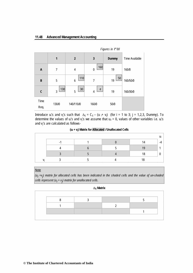
Introduce ui’s and vj’s such that ∆ij = Cij – (u i+ vj) (for i = 1 to 3; j = 1,2,3, Dummy). To determine the values of ui’s and vj’s we assume that u3 = 0, values of other variables i.e. ui’s and vj’s are calculated as follows-
(ui + vj) Matrix for Allocated / Unallocated Cells
ui
-1 1 0 14 -4
4 6 5 19 1
3 5 4 18 0
vj 3 5 4 18
Note (ui +vj) matrix for allocated cells has been indicated in the shaded cells and the value of un-shaded cells represent (ui + vj) matrix for unallocated cells.
Δij Matrix
8 3 5
1 2
1
130
50 110
30
160
e
© The Institute of Chartered Accountants of India
The Transportation Problem 11.49
Since all Δij cells value are positive, therefore the initial solution obtained above is optimal. The allocation of projects to auditors and their billing amount is given below-
Auditor Project Working Hours Rate per hour (`) Billing Amount (`) A 3 160 1,900 3,04,000 B 2 110 1,300 1,43,000 C 1 130 1,600 2,08,000 C 2 30 1,400 42,000
Total Billing 6,97,000
Hence, the maximum total billing during the next month will be `6,97,000/- Question-13 A company has three factory and four customers. The company furnishes the following schedule of profit per unit on transportation of goods to the customers in rupees:
Factory Customers
Supply A B C D P 40 25 22 33 100 Q 44 35 30 30 30 R 38 38 28 30 70
Demand 40 20 60 30 150 / 200
You are required to solve the transportation problem to maximize the profit and determine the resultant optimal profit.
Solution:
Convert the given profit matrix into a loss matrix by subtracting each element of the matrix from the highest value viz.44.The resulting loss matrix is as follows:
Loss Matrix
Factory Customers
Supply A B C D P 4 19 22 11 100 Q 0 9 14 14 30 R 6 6 16 14 70
Demand 40 20 60 30 150 / 200
© The Institute of Chartered Accountants of India
11.50 Advanced Management Accounting
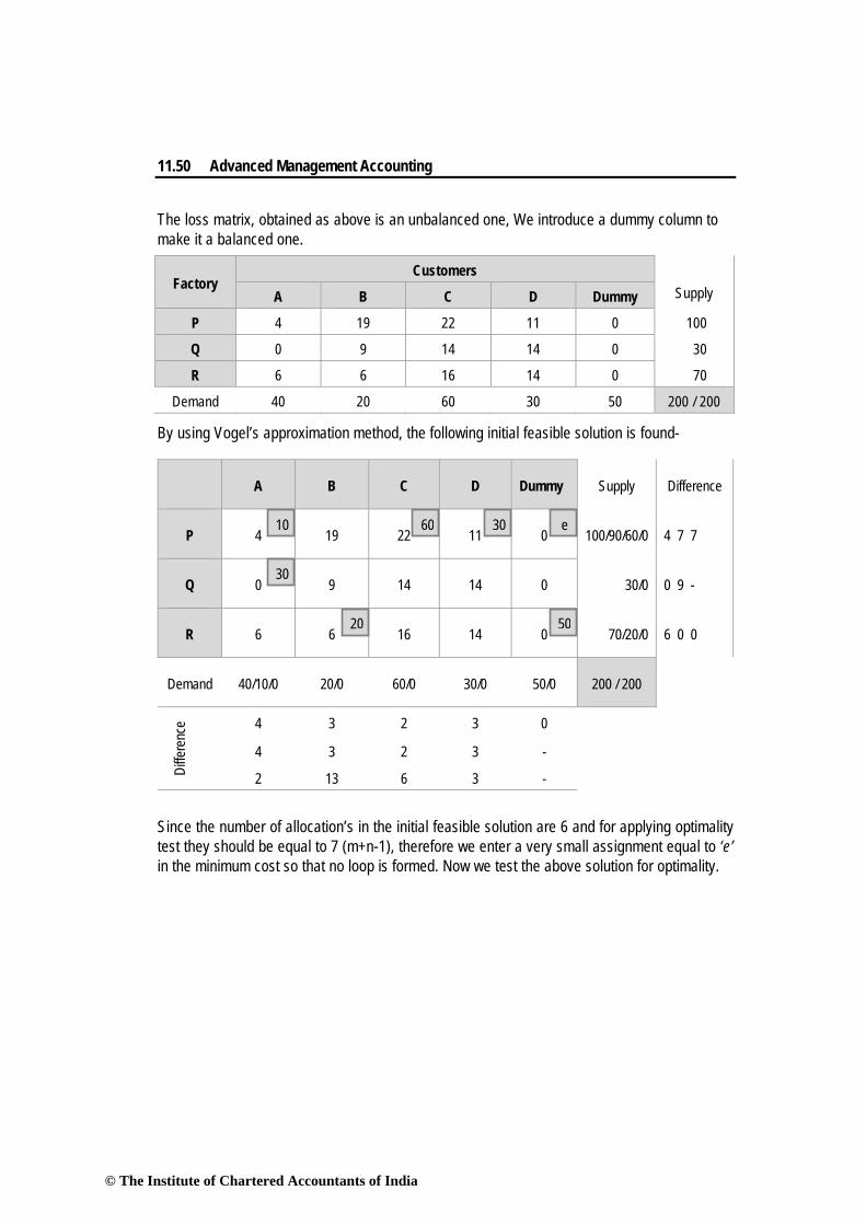
The loss matrix, obtained as above is an unbalanced one, We introduce a dummy column to make it a balanced one.
Factory Customers
Supply A B C D Dummy
P 4 19 22 11 0 100
Q 0 9 14 14 0 30
R 6 6 16 14 0 70
Demand 40 20 60 30 50 200 / 200
By using Vogel’s approximation method, the following initial feasible solution is found-
A B C D Dummy Supply Difference
P 4 19 22 11 0 100/90/60/0 4 7 7
Q 0 9 14 14 0 30/0 0 9 -
R 6 6 16 14 0 70/20/0 6 0 0
Demand 40/10/0 20/0 60/0 30/0 50/0 200 / 200
Diffe
renc
e 4 3 2 3 0
4 3 2 3 -
2 13 6 3 -
Since the number of allocation’s in the initial feasible solution are 6 and for applying optimality test they should be equal to 7 (m+n-1), therefore we enter a very small assignment equal to ‘e’ in the minimum cost so that no loop is formed. Now we test the above solution for optimality.
10 60
20
30
30
50
e
© The Institute of Chartered Accountants of India

The Transportation Problem 11.51
(ui + vj) Matrix for Allocated / Unallocated Cells
ui
4 6 22 11 0 0
0 2 18 7 -4 -4
4 6 22 11 0 0
vj 4 6 22 11 0
Note (ui +vj) matrix for allocated cells has been indicated in the shaded cells and the value of un-shaded cells represent (ui + vj) matrix for unallocated cells.
Now we calculate Δij = Cij – (ui +vj) for non basic cells which are given in the table below:
Δij Matrix
13
7 -4 7 4
2 -6 3
Since, there are two negative cell values in the above Δij Matrix, so we have to do re allocation by making a loop and allocate at the cell which has the maximum negative value. The re-allocation will be as follows-
10 60
-50
30 e
+50
30
20
+50
50
-50
Revised allocations (improved initial solution) are as follows-
10 10 30 50
30
20 50
© The Institute of Chartered Accountants of India
11.52 Advanced Management Accounting
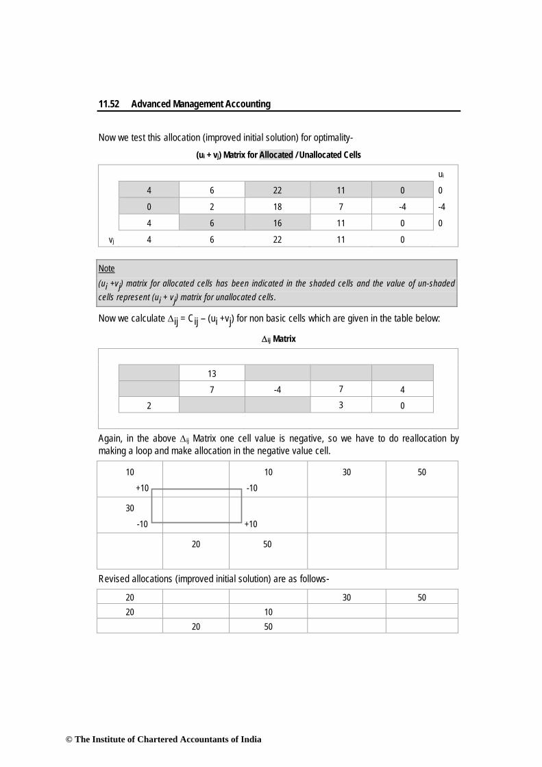
Now we test this allocation (improved initial solution) for optimality- (ui + vj) Matrix for Allocated / Unallocated Cells
ui
4 6 22 11 0 0
0 2 18 7 -4 -4
4 6 16 11 0 0
vj 4 6 22 11 0
Note (ui +vj) matrix for allocated cells has been indicated in the shaded cells and the value of un-shaded cells represent (ui + vj) matrix for unallocated cells.
Now we calculate Δij = Cij – (ui +vj) for non basic cells which are given in the table below:
Δij Matrix
13
7 -4 7 4
2 3 0
Again, in the above Δij Matrix one cell value is negative, so we have to do reallocation by making a loop and make allocation in the negative value cell.
10
+10
10
-10
30 50
30
-10
+10
20 50
Revised allocations (improved initial solution) are as follows-
20 30 50 20 10 20 50
© The Institute of Chartered Accountants of India
The Transportation Problem 11.53
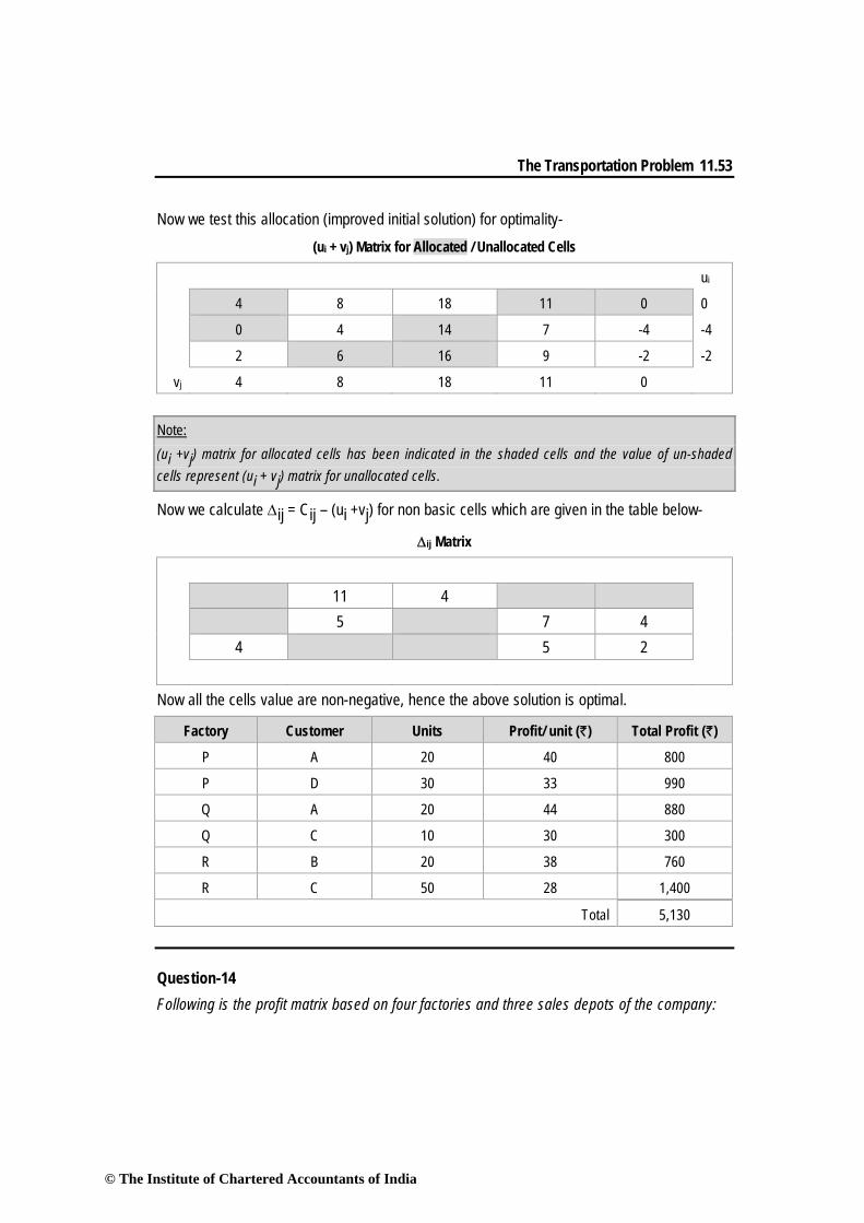
Now we test this allocation (improved initial solution) for optimality- (ui + vj) Matrix for Allocated / Unallocated Cells
ui
4 8 18 11 0 0
0 4 14 7 -4 -4
2 6 16 9 -2 -2
vj 4 8 18 11 0
Note: (ui +vj) matrix for allocated cells has been indicated in the shaded cells and the value of un-shaded cells represent (ui + vj) matrix for unallocated cells.
Now we calculate Δij = Cij – (ui +vj) for non basic cells which are given in the table below-
Δij Matrix
11 4
5 7 4
4 5 2
Now all the cells value are non-negative, hence the above solution is optimal.
Factory Customer Units Profit/ unit (`) Total Profit (`)
P A 20 40 800
P D 30 33 990
Q A 20 44 880
Q C 10 30 300
R B 20 38 760
R C 50 28 1,400
Total 5,130 Question-14 Following is the profit matrix based on four factories and three sales depots of the company:
© The Institute of Chartered Accountants of India
11.54 Advanced Management Accounting
Factory Sales Depot Availability
S1 S2 S3
F1 6 6 1 10
F2 -2 -2 -4 150
F3 3 2 2 50
F4 8 5 3 100
Requirement 80 120 150 350 / 310
Determine the most profitable distribution schedule and the corresponding profit, assuming no profit in case of surplus production.
Solution: The given transportation problem is an unbalanced one and it is a maximisation problem. As a first step, we will balance this transportation problem, by adding a dummy factory, assuming no profit in case of surplus production.
Factory Sales Depot Availability
S1 S2 S3
F1 6 6 1 10
F2 -2 -2 -4 150
F3 3 2 2 50
F4 8 5 3 100
Dummy 0 0 0 40
Requirement 80 120 150 350 / 350 We shall now convert the above transportation problem (a profit matrix) into a loss matrix by subtracting all the elements from the highest value in the table i.e. 8. Therefore, we shall apply the VAM to find initial solution.
© The Institute of Chartered Accountants of India
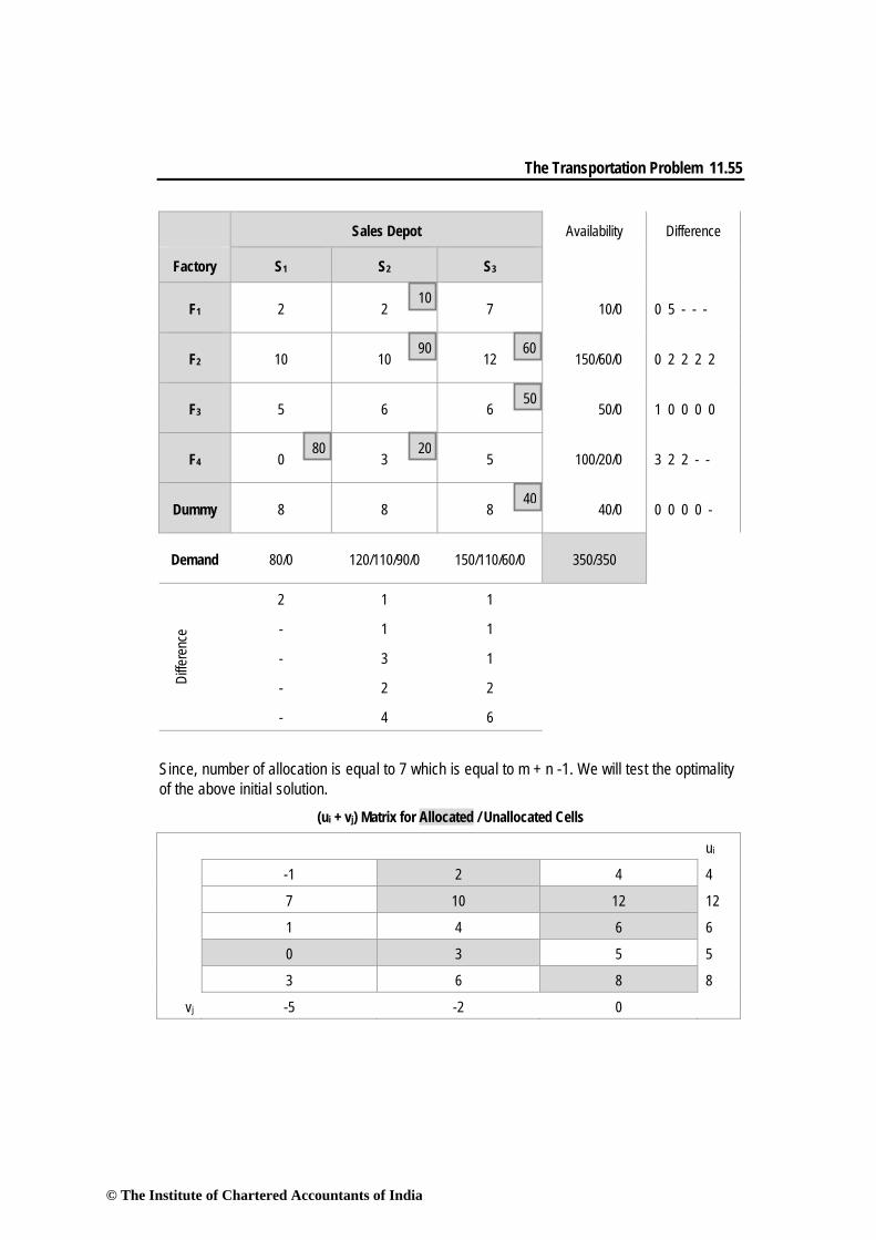
The Transportation Problem 11.55
Sales Depot Availability Difference
Factory S1 S2 S3
F1 2 2 7 10/0 0 5 - - -
F2 10 10 12 150/60/0 0 2 2 2 2
F3 5 6 6 50/0 1 0 0 0 0
F4 0 3 5 100/20/0 3 2 2 - -
Dummy 8 8 8 40/0 0 0 0 0 -
Demand 80/0 120/110/90/0 150/110/60/0 350/350
Diffe
renc
e
2 1 1
- 1 1
- 3 1
- 2 2
- 4 6 Since, number of allocation is equal to 7 which is equal to m + n -1. We will test the optimality of the above initial solution.
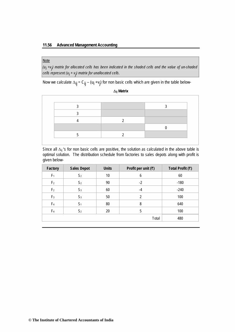
(ui + vj) Matrix for Allocated / Unallocated Cells
ui
-1 2 4 4
7 10 12 12
1 4 6 6
0 3 5 5
3 6 8 8
vj -5 -2 0
20
10
90
80
60
50
40
© The Institute of Chartered Accountants of India
11.56 Advanced Management Accounting
Note (ui +vj) matrix for allocated cells has been indicated in the shaded cells and the value of un-shaded cells represent (ui + vj) matrix for unallocated cells.
Now we calculate Δij = Cij – (ui +vj) for non basic cells which are given in the table below-
Δij Matrix
3 3
3
4 2
0
5 2
Since all Δij ‘s for non basic cells are positive, the solution as calculated in the above table is optimal solution. The distribution schedule from factories to sales depots along with profit is given below-
Factory Sales Depot Units Profit per unit (`) Total Profit (`)
F1 S2 10 6 60
F2 S2 90 -2 -180
F2 S3 60 -4 -240
F3 S3 50 2 100
F4 S1 80 8 640
F4 S2 20 5 100
Total 480
© The Institute of Chartered Accountants of India


![Transportation Problem - ULisboaweb.tecnico.ulisboa.pt/~mcasquilho/CD_Casquilho/PRINT/...Transportation Problem [:8] 3 Any problem having the above structurecan beconsidered a TP,](https://static.fdocuments.in/doc/165x107/5e753e5b11ea724b977b7d81/transportation-problem-mcasquilhocdcasquilhoprint-transportation-problem.jpg)