E u r . J P h v 10 ( I Y X Y ) 99-1115 Prmled In the U K

99

Chaos in a dripping faucet

H N Nufiez Yepezts, A L Salas Britots, C A Vargas'' and L A Vicente5 f Departamento de Fisica, Facultad de Ciencias, Universidad Nacional Autonoma de Mexico, Apartado Postal 21-726, Mexico 04000 D F, Mexico $ Departamento de Ciencias Basicas, Universidad Autonoma Metropolitana-Azcapotzalco, Mexico D F, Mexico.

Facultad de Quimica, Universidad Nacional Autonoma de Mexico. Mexico D F, Mexico

Received 6 April 1988, in final form 10 August 1988

Abstract. An advanced undergraduate experiment on the chaotic behaviour of a dripping faucet is presented. The experiment can be used for the demonstration of typical features of chaotic phenomena and also allows the advanced physics student to learn about the use of microcomputers as data-taking devices. For convenience a brief introduction to the basic concepts of non-linear dynamics and to the period-doubling route to chaos are included.

1. Introduction Chaodynamics is a recent area of research (Ott 1981, Ford 1983, Bai Lin 1984, Jensen 1987); even its name is recent (Andrey 1986). It concerns the occurrence of complex and seemingly random pheno- mena in non-linear but otherwise deterministic systems. Common examples of this behaviour include the results of tossing a coin, or the swirling paths of leaves falling from a tree on a windy day. Similar aperiodic phenomena have been observed in an impressive number of experimental systems, even in some previously thought to be very well understood, as is the case of the driven pendulum (Koch et a/ 1983). Electrical, optical, mechanical, chemical, hydrodynamical and biological systems can all exhibit the kind of dynamical instabilities that produce chaotic behaviour (Jensen 1987 and refer- ences therein). Despite this, recent discoveries in the field of non-linear dynamics are still not well known to many undergraduate physics students.

With the above ideas in mind, we have developed an experiment that can be useful for introducing some of the ideas and methods used in the descrip- tion of non-linear chaotic systems. Our experiment follows the work of Martien et a/ (1985). based on a

Resumen. Se propone un experimento sobre el comportamiento caotico del goteo en una llave mal cerrada. Este resulta ut i1 para la demonstracion de caracteristicas tipicas de 10s fenomenos caoticos, y permite que 10s estudiantes de fisica aprendan a usar una microcomputadora para la toma de datos en un experimento. Hemos creido conveniente incluir una breve introduccion a la dinamica no lineal y. en particular, a la aparicion de caos por sucesivas bifurcaciones subarmonicas.

suggestion of Rossler (1977), which shows that drops falling from a leaky faucet behave chaotically under appropriate conditions. Other experiments, demonstrations or computer simulations have been recently proposed to introduce students to the field of non-linear phenomena (e.g. Berry 1981, Viet et a/ 1983. Salas Brito and Vargas 1986, Briggs 1987), but curiously none of them deals with liquids despite the fact that much original work has been done on such systems. In our experiment the students investigate the dripping behaviour of a leaky faucet, a system which remains incompletely understood and hence may still offer some surprises to both teachers and students. In this system, the students can measure the time interval between successive drops, the drip interval-as we, following Martien et a/ (1985), will call it-as a function of the flow rate of water.

The students become acquainted with the con- cepts of non-linear dynamics (as deterministic chaos, attractors, subharmonic bifurcations, and the like) by reading the basic literature, paying particu- lar attention to the logistic map (May 1976, Feigenbaum 1980, Hofstadter 1981, Schuster 1984, Jensen 1987). Then, since many aspects of this

100 H N Nuriez Ybpez et a1

mapping are common to a large class of dynamical systems showing chaotic behaviour, they are encour- aged to explore i t on a microcomputer to obtain firsthand experience of the behaviour of a chaotic system, before they begin the experiment.

In the following we summarise the experimental set-up and show the results obtained so far in our laboratories. Since the dripping faucet seems to follow the period-doubling route to chaos (Martien et a1 1985), after a brief introduction to illustrate the basic concepts of the field, in Q 2 we examine in some detail the logistic map, a paradigmatic exam- ple of a system following such a route to chaos. In Q 3 we describe our experimental device and show the return maps obtained from the data collected. These data confirm the existence of a sequence of period doublings in the system, at least up to period four, before the onset of chaos. Finally, we present our conclusions in D 4.

2. Basic concepts and the period-doubling route to chaos Let us first introduce some basic notions and termi- nology of non-linear dynamics. Consider an harmo- nically driven pendulum: given the frequency and strength of the driving force, the motion of the system is cpmp!etely determined if the angle 0 and angular speed 0 of the pendulum are known. These variables can be used as coordinates in the phase space of the pendulum; as it swings back and forth, the point representing its state moves along an orbit in phase space. For example, if the strength of the driving force vanishes, due to the effect of friction, no matter how we start its motion the pendulum will come to rest at its point of stable equilibrium after a number of oscillations. From the point of view of phase space, the orbit spirals to the fixed point at the origin. The motion is quite different for non-zero values of the driving force; in this case the pendulum settles to a stationary oscillation with the same frequency as the external driving force. These sta- tionary motions in which the system settles after the transients have died out are examples of attractors, a term which conveys the idea that many nearby orbits are ‘attracted’ to them. We have mentioned two types of attractors, a stable fixed point and a stable limit cycle, but there exists a more complicated attractor, the so-called strange attractors which only occur in dissipative non-linear systems. They cap- ture the solution of a deterministic system into a perfectly defined region of phase space, but in which there is a very complex structure (these objects are usually fractals) and the motion shows every feature associated with random motion. Such behaviour is a manifestation of the very sensitive dependence on the initial conditions developed by the system (Ruelle 1980). The existence of strange attractors is one of the fingerprints of chaos i.e. the loss of long-

term predictability in a supposedly deterministic system.

Various attractors may be present in the long- term behaviour of a dynamical system; in most. its presence or absence is governed by the value of a single control parameter. For example, the magni- tude the driving force determines if the pendulum settles to a point or to a limit cycle (or possibly even to a more complex attractor (D’Humieres e f a1 1982)). In the case of the dripping faucet, it is the flow rate of water which governs its dynamics: for low values of flow. the dripping is simply periodic and the system is attracted to a stable fixed point: but for much larger values of flow, strange attractors can appear. The succession of stationary states which a system follows prior of the onset of chaos, as the control parameter is varied, determines what is called the route to chaos followed by the system (Kadanoff 1983). The dripping faucet seems to fol- low the period-doubling route to chaos (Martien et a1 1985). We will explain this route in some detail below.

The evolution of a dynamical system can be des- cribed in either continuous time (a flow) or in discrete time (a mapping). The pendulum is a good example of a system that may be described by a flow in phase space-although it can also be described by a mapping (Testa et a1 1982). On the other hand. the sequence of drip intervals in a leaky faucet is natur- ally described by a discrete map. For any given value of the dripping rate. a plot of the next drip interval versus the previous one can give a clear idea of its dripping behaviour and of the possible existence of attractors. This is the representation we use for the data obtained in the experiment (see figure 5); i t is called a return or Poincare map.

As an illustration of some of these ideas. and because they offer perhaps the simplest examples of systems undergoing a period-doubling transition to chaos, we shall consider iterative processes of the form

where f ( x ) is a continuous function defined in a suitable one-dimensional interval. Discussing only one-dimensional mappings as (1) is not as restrictive as it may seem at first. since it can be viewed as a discrete time version of a continuous but dissipative dynamical system. The dissipative terms shrink the volume of phase space occupied by the system until it becomes effectively one-dimensional. In this instance it can be modelled, at least in its universal qualitative features, by a simple mapping as (1) (Collet and Eckmann 1980). In fact, such iterations have been advocated frequently as qualitative models for many complex physical systems, from the behaviour of a driven non-linear oscillator (Linsay 1981, Testa et a1 1982) to the onset of turbulence in the Rayleigh-Benard phenomena (Gollub and Benson 1980). Most of the results here do not

Chaos in a dripping faucet 101

0 8

- F

0 4

0 0 4 0 8

I C )

0 . 8 .

z 0 4 -

0 0 4 0.0 Xn

l b )

0 . 8 .

0 . 4 .

0 0 4 0 8

0 0 4 0 8 X”

Figure 1. Return maps, i.e. plots of x,l-, versus x,, for large values of n , obtained from the logistic map for different values of U : ( a ) U = 1.5; ( b ) p = 3.3; (c) U = 3.5; ( d ) U = 3.8. This illustrates the dynamics of the map up to the four cycle as well as the chaotic attractor for p > p x .

depend on the precise form of the function f ( x ) . as long as it has a single quadratic maximum but to be specific we will analyse the dynamics of the logistic map. This mapping is defined by

f(x) = / d l - x ) ( 2 )

where 0+<4 is a parameter measuring the strength of the non-linearity. With this choice for f ( x ) . equation (1) describes a non-linear and non- invertible map of the unit interval on itself. The evolution of the sequence of x, generated by this simple equation exhibits a transformation from per- iodic to chaotic behaviour as the control parameter p is increased. Let us see how this occurs. The behaviour of the sequence of iterates is trivial when p = 0: for every initial value x,, all the iterates are zero. We can say then that the solution quickly reaches an attractor, the single point x=O; this is called a period-one cycle, orbit or attractor. For values ofp between 0 and 1, the large n behaviour of the x, is identical; they approach the point x = 0 after a certain number of steps. But for larger values of p the dynamics is much more interesting as can be easily verified using a hand-held calculator. Various types of stationary solutions of the logistic map are exemplified by figures 1 and 2.

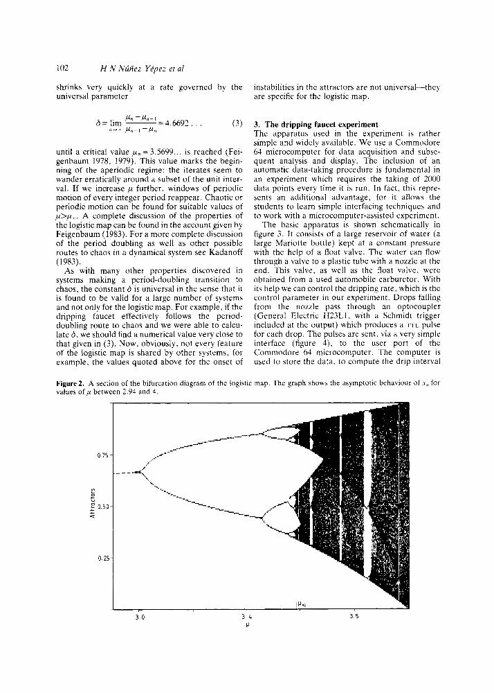
Figure 1 shows return maps (plots of x , , , versus x , ) for ,U = 1.5, 3.3. 3.5 and 3.8. The successive

appearance of attractors of period one, two. four and of a one-dimensional chaotic attractor can be appreciated in these plots. Figure 2 illustrates this kind of behaviour in a different and more global way; it shows a plot of the large n behaviour of the iterates (i.e. the attractors) of the logistic map as a function of the value of p. This graph gives a ‘pictorial meaning’ to the way the onset of chaos occurs via a sequence of ‘pitchfork’ (period- doubling) bifurcations as the value of p changes. I t also shows the critical dependence of the behaviour with the value of this parameter. For values of p between 1 and 3 , and almost all initial values x ( , , there is a single point attractor (figure l(a)). Then. as p is increased between 3 and 4, the dynamics changes in surprising ways. First, for 3 < p S ( l + G) the stationary solution bifurcates to a period-two attractor-the period of the solution has doubled and its frequency halved, hence the names of period-doubling or subharmonic bifurcation given to the phenomena-as can be seen in the bifurcation diagram (figure 2), where the solution hops back and forth between the upper and lower branches of the pitchfork, and in figure l (b ) . As p is increased further. the solution bifurcates again to a period- four attractor, then to a period-eight attractor and so on. This sequence (or cascade) of bifurcations continues indefinitely, but the interval of values of p in which a given periodic orbit acts as an attractor

102 H N Nlinez Ykpez et a1

shrinks very quickly at a rate governed by the universal parameter

6 = lim “4.6692.. . P E -Pn-l n-= ,P,+, -P,,

(3)

until a critical value = 3.5699.. . is reached (Fei- genbaum 1978, 1979). This value marks the begin- ning of the aperiodic regime: the iterates seem to wander erratically around a subset of the unit inter- val. If we increase p further, windows of periodic motion of every integer period reappear. Chaotic or periodic motion can be found for suitable values of ,u>pm. A complete discussion of the properties of the logistic map can be found in the account given by Feigenbaum (1983). For a more complete discussion of the period doubling as well as other possible routes to chaos in a dynamical system see Kadanoff (1983).

As with many other properties discovered in systems making a period-doubling transition to chaos, the constant d is universal in the sense that it is found to be valid for a large number of systems and not only for the logistic map. For example, if the dripping faucet effectively follows the period- doubling route to chaos and we were able to calcu- late 8, we should find a numerical value very close to that given in (3). Now, obviously, not every feature of the logistic map is shared by other systems, for example, the values quoted above for the onset of

instabilities in the attractors are not universal-they are specific for the logistic map.

3. The dripping faucet experiment The apparatus used in the experiment is rather simple and widely available. We use a Commodore 64 microcomputer for data acquisition and subse- quent analysis and display. The inclusion of an automatic data-taking procedure is fundamental in an experiment which requires the taking of 2000 data points every time it is run. In fact. this repre- sents an additional advantage, for it allows the students to learn simple interfacing techniques and to work with a microcomputer-assisted experiment.

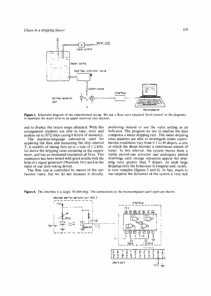
The basic apparatus is shown schematically i n figure 3. It consists of a large reservoir of water (a large Mariotte bottle) kept at a constant pressure with the help of a float valve. The water can flow through a valve to a plastic tube with a nozzle at the end. This valve, as well as the float valve, were obtained from a used automobile carburetor. With its help we can control the dripping rate, which is the control parameter in our experiment. Drops falling from the nozzle pass through an optocoupler (General Electric H23L1, with a Schmidt trigger included at the output) which produces a TTL pulse for each drop. The pulses are sent, via a very simple interface (figure 4) , to the user port of the Commodore 64 microcomputer. The computer is used to store the data, to compute the drip interval

Figure 2. A section of the bifurcation diagram of the logistic map. The graph shows the asymptotic behaviour of x,, for values of ,U between 2.94 and 4.

0 75

c v

2

2 0 5 0 4 + c

0 . 2 5

3.0 3 4 3 8 P

Chaos in a dripping faucet 103

Woter In le t

~- " - M o d i f i e d carburetor va lve

Interface

Emlt ter -detector p a r

Mlcrocomputer

Figure 3. Schematic diagram of the experimental set-up. We use a float valve (marked 'level control' in the diagram) to maintain the water level in an upper reservoir (not shown).

and to display the return maps obtained. With this arrangement students are able to take, store and analyse up to 3072 drips (using 6 Kbyte of memory).

The machine-language subroutine used for acquiring the data and measuring the drip interval T, is capable of taking data up to a rate of 1.2 kHz, far above the dripping rates occurring in the experi- ment, and has an estimated resolution of 50 p . This estimation has been tested with good results with the help of a signal generator (Wavetek 181) used as the input of our data-taking device.

The flow rate is controlled by means of the car- buretor valve, but we do not measure it directly.

preferring instead to use the valve setting as an indicator. The program we use to analyse the data computes a mean dripping rate. The mean dripping rates students are able to investigate under experi- mental conditions vary from 0.1 to 40 drips/s, a rate at which the drops become a continuous stream of water. In this interval, the system moves from a stable period-one attractor and undergoes period doublings until strange attractors appear for drip- ping rates greater than 7 drips/s. At such large dripping rates the behaviour is irregular and, surely, is very complex (figures 5 and 6). In fact, much to our surprise the dynamics of the system is very rich

Figure 4. The interface is a single 74LSOO chip. The connections to the microcomputer user's port are shown

Motched eml t ter -detector par H23 L1 """""

I I I

I I I I I I I l I

User's p o r t

104 H N Nunez Ykpez et a1

412 4

l -.,. i

L

l , l l 384- , I

384 41 2 440 0 30 60 0 64 128

1 1 , l

105 i l I l v "" - i 158 ,

105 114 123 0 33 66 158 173 188

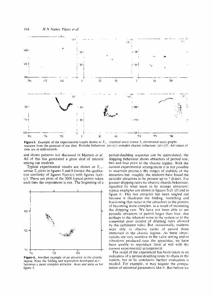
Figures. Example of the experimental results shown as T,,,, (vertical axes) versus T,, (horizontal axes) graphs redrawn from the printout of our data. Periodic behaviour, (o) - (c) : complex chaotic behaviour. ( d ) - ( f ) , AI1 values of time are in milliseconds.

and shows patterns not discussed in Martien et al. All of this has generated a great deal of interest among our students.

Typical experimental results are shown as T,,,, versus T,, plots in figures 5 and 6 (notice the qualita- tive similarity of figures 5(a)-(c) with figures l (a ) - (c). These are plots of the 2000 typical points taken each time the experiment is run. The beginning of a

114 ; I I I I

11 4 122 130 Figure 6. Another example of an attractor in the chaotic region. Note the folding and separation developed as i t becomes a more complex attractor. Axes and units as for figure 5 .

period-doubling sequence can be appreciated; the dripping behaviour shows attractors of period one, two and four prior to the chaotic regime. With the current experimental arrangement it is not possible to ascertain precisely the ranges of stability of the attractors but. roughly, the students have found the periodic attractors to be present up to 7 dripsis. For greater dripping rates we observe chaotic behaviour, signalled by what seem to be strange attractors: typical examples are shown in figures 5(d)-V) and in figure 6. This last attractor has been singled out because it illustrates the folding, stretching and fractioning that occur in the attractors in the process of becoming more complex, as a result of increasing the dripping rate. We have not been able to see periodic attractors of period larger than four. due perhaps to the inherent noise in the system or to the somewhat poor control of dripping rates allowed by the carburetor valve. But, occasionally, students were able to observe cycles of period three immersed in the chaotic regime. As these obser- vations are very sensitive to the valve setting and to vibrations produced near the apparatus. we have been unable to reproduce them at will with the current experimental arrangement.

The result of the experiment has been taken as an indication of a period-doubling route to chaos in the system, but to be conclusive further evaluation is needed. For example, i t may require the compu- tation of universal parameters like d. But before we

Chaos in a dripping faucet 105

can determine such parameters we must be able to measure with greater confidence the stability inter- vals of the attractors and to discern at least a period- eight attractor.

As figures 5 and 6 show, the aperiodic regime exhibits patterns of behaviour which seem to have an underlying one-dimensional structure somewhat blurred by the noise in the system. This quasi-one- dimensional appearance of the attractors is an indi- cator of chaotic behaviour as a characteristic of the system and not a result of external noise generated, for example. by the carburetor valve or produced by small air currents. On the other hand, these results show that a qualitative model in terms of a one-dimensional mapping may be appropriate. In fact. to analyse the results of their experiment Martien et a/ proposed a very simple one- dimensional analogue model. It is worth mentioning here that the system exhibits hysteresis and the bifurcation points may differ for increasing and decreasing dripping rates. Despite the fact that the system is expected to show hysteresis, we believe our observations to be due mainly to the valve used to control the flow of water. We are now trying to improve the arrangement and to use a good needle valve in order to determine this.

4. Conclusions In summary, we have presented an experiment in which students can investigate the non-linear behav- iour and the route to chaos in a dripping faucet. Students are able to observe a sequence of period doublings preceding chaos and the existence of a chaotic regime with various types of strange attrac- tors. They can also convince themselves that despite the large number of variables involved in the pheno- menon i t can be qualitatively modelled by a one- dimensional mapping (although we may expect bet- ter agreement with a mapping of greater dimensio- nality).

In view of the above results, and to the relative simplicity of the experimental arrangement, we think that this system is very suitable for introducing the concept of non-linear dynamics and the tech- niques for its experimental study. The experiment is a very good example of the type of behaviour possible in classical dynamic systems. Our experi- mental set-up can also be useful as an exhibit or to inform conferences addressing wider audiences. On the other hand, when used in an open-ended investi- gation. i t has allowed our students to explore the many features of the transition to chaos at their own

level and interest. Another useful feature of the experiment is that it allows advanced physics stu- dents to learn about simple interfacing techniques and the use of microcomputers as data-taking devices in physics experiments.

Finally, we must say that a similar experiment is being developed at Universidad Simon Bolivar (Venezuela) by Professor C L Ladera at the sugges- tion of one of us (ALSB).

Acknowledgments We wish to thank C Carbajal and J Sandria for developing the machine-language subroutine used by the data-taking procedure and for their help in setting up the experiment. We also wish to thank F D Micha for her help in revising the manuscript.

References Andrey L 1986 Prog. Theor. Phys. 75 1258 Bai Lin H 1984 Chaos (Singapore: World Scientific) Berry M V 1981 Eur. J . Phys. 2 91 Briggs K 1987 A m . J . Phys. 55 1083 Collet P and Eckmann J P 1980 Iterated Maps of [he

D'Humieres D, Beasley M R. Huberman B A and

Feigenbaum M J 1978 J . Stat. Phys. 19 25

"-1980 Los Alamos Sci. 1 4

Ford J 1983 Phys. Today 36 (4) 40 Gollub J P and Benson S V 1980 J . Nuid Mech. 100 449 Hofstadter D R 1981 Sci. A m . 245 22 (November) Jensen R V 1987 A m . Sci. 75 168 Kadanoff L P 1983 Phys. Today 36 (12) 46 Koch B P. Leven R W. Pompe B and Wilke G 1983

Linsay R S 1981 Phys. Reo. Lett. 47 1349 Martien P. Pope S C. Scott P L and Shaw R S 1985

May R M 1976 Nature 261 459 Ott E 1981 Rev. Mod. Phys. 53 635 Rossler 0 1977 in Synergerm: a workshop ed. H Haken

Ruelle D 1980 L a Recherche 11 133 Salas Brito A L and Vargas C 1986 Reo. M e x . Fis. 32

Schuster H 1984 Deterministlc Chaos: A n Introduction

Testa J . Perez J and Jeffries C 1982 Phys. Reo. Letr. 48

Vlet 0. Wesfreid J E and Guyon E 1983 Eur. J . Phys. 4

Interval as Dynamical Systems (Boston: Birkhauser)

Libchaber A 1982 Phys. Rev. A 26 3483

"-1979 J . Slat. Phys. 21 669

-1983 Physics 7D 16

Phys. Lett 96A 219

Phys. Lett. llOA 399

(Berlin: Springer) p 174

357

(Weinhein: Physik Verlag)

714

72