C++ for Finance
264
Financial Numerical Recipes in C ++ . Bernt Arne Ødegaard June 2014
-
Upload
karan-malhotra -
Category
Documents
-
view
53 -
download
7
description
C++ as applied to quantitative finance
Transcript of C++ for Finance

Financial Numerical Recipes in C++.
Bernt Arne Ødegaard
June 2014

Contents
1 On C++ and programming. 5
1.1 Compiling and linking . . . . . . . . . . . . . . . 51.2 The structure of a C++ program . . . . . . . . . 6
1.2.1 Types . . . . . . . . . . . . . . . . . . . . 61.2.2 Operations . . . . . . . . . . . . . . . . . 61.2.3 Functions and libraries . . . . . . . . . . . 71.2.4 Templates and libraries . . . . . . . . . . 71.2.5 Flow control . . . . . . . . . . . . . . . . . 81.2.6 Input Output . . . . . . . . . . . . . . . . 81.2.7 Splitting up a program . . . . . . . . . . . 81.2.8 Namespaces . . . . . . . . . . . . . . . . . 9
1.3 Extending the language, the class concept. . . . 91.3.1 date, an example class . . . . . . . . . . . 10
1.4 Const references . . . . . . . . . . . . . . . . . . . 161.5 Other C++ concepts . . . . . . . . . . . . . . . . . 16
2 Matrix Tools 17
2.1 The first screen . . . . . . . . . . . . . . . . . . . 182.2 Linear algebra . . . . . . . . . . . . . . . . . . . . 18
2.2.1 Basic matrix operations . . . . . . . . . . 182.2.2 Arithmetic Matrix Operations. . . . . . . 19
2.3 Solving linear equations . . . . . . . . . . . . . . 222.4 Element by element operations . . . . . . . . . . 242.5 Function definitions . . . . . . . . . . . . . . . . 242.6 m files . . . . . . . . . . . . . . . . . . . . . . . . 242.7 Flow control . . . . . . . . . . . . . . . . . . . . . 242.8 Plotting . . . . . . . . . . . . . . . . . . . . . . . 242.9 Libraries . . . . . . . . . . . . . . . . . . . . . . . 252.10 References . . . . . . . . . . . . . . . . . . . . . . 25
3 The value of time 26
3.1 Present value . . . . . . . . . . . . . . . . . . . . 263.2 One interest rate with annual compounding . . . 27
3.2.1 Internal rate of return. . . . . . . . . . . . 303.3 Continously compounded interest . . . . . . . . . 34
3.3.1 Present value . . . . . . . . . . . . . . . . 353.4 Further readings . . . . . . . . . . . . . . . . . . 35
4 Bond Pricing with a flat term structure 36
4.1 Flat term structure with discrete, annual com-pounding . . . . . . . . . . . . . . . . . . . . . . 374.1.1 Bond Price . . . . . . . . . . . . . . . . . 374.1.2 Yield to maturity . . . . . . . . . . . . . . 384.1.3 Duration . . . . . . . . . . . . . . . . . . . 414.1.4 Measuring bond sensitivity to interest
rate changes . . . . . . . . . . . . . . . . . 434.2 Continously compounded interest . . . . . . . . . 474.3 Further readings . . . . . . . . . . . . . . . . . . 50
5 The term structure of interest rates and an object lesson 51
5.1 The interchangeability of discount factors, spotinterest rates and forward interest rates . . . . . 52
5.2 The term structure as an object . . . . . . . . . . 555.2.1 Base class . . . . . . . . . . . . . . . . . . 555.2.2 Flat term structure. . . . . . . . . . . . . 57
5.3 Using the currently observed term structure. . . . 585.3.1 Linear Interpolation. . . . . . . . . . . . . 595.3.2 Interpolated term structure class. . . . . . 61
5.4 Bond calculations with a general term structureand continous compounding . . . . . . . . . . . . 64
6 The Mean Variance Frontier 67
6.1 Setup . . . . . . . . . . . . . . . . . . . . . . . . 676.2 The minimum variance frontier . . . . . . . . . . 696.3 Calculation of frontier portfolios . . . . . . . . . 696.4 The global minimum variance portfolio . . . . . . 726.5 Efficient portfolios . . . . . . . . . . . . . . . . . 726.6 The zero beta portfolio . . . . . . . . . . . . . . . 736.7 Allowing for a riskless asset. . . . . . . . . . . . . 736.8 Efficient sets with risk free assets. . . . . . . . . . 746.9 Short-sale constraints . . . . . . . . . . . . . . . . 756.10 The Sharpe Ratio . . . . . . . . . . . . . . . . . . 756.11 Equilibrium: CAPM . . . . . . . . . . . . . . . . 76
6.11.1 Treynor . . . . . . . . . . . . . . . . . . . 766.11.2 Jensen . . . . . . . . . . . . . . . . . . . 76
6.12 Working with Mean Variance and CAPM . . . . . 766.13 Mean variance analysis using matrix libraries . . 77
7 Futures algoritms. 81
7.1 Pricing of futures contract. . . . . . . . . . . . . 81
8 Binomial option pricing 82
8.1 Options . . . . . . . . . . . . . . . . . . . . . . . 828.2 Pricing . . . . . . . . . . . . . . . . . . . . . . . . 828.3 Multiperiod binomial pricing . . . . . . . . . . . 85
9 Basic Option Pricing, the Black Scholes formula 89
9.1 The formula . . . . . . . . . . . . . . . . . . . . . 909.2 Understanding the why’s of the formula . . . . . 92
9.2.1 The original Black Scholes analysis . . . . 939.2.2 The limit of a binomial case . . . . . . . . 939.2.3 The representative agent framework . . . 93
9.3 Partial derivatives. . . . . . . . . . . . . . . . . . 939.3.1 Delta . . . . . . . . . . . . . . . . . . . . . 939.3.2 Other Derivatives . . . . . . . . . . . . . . 949.3.3 Implied Volatility. . . . . . . . . . . . . . 96
9.4 References . . . . . . . . . . . . . . . . . . . . . . 98
10 Warrants 99
10.1 Warrant value in terms of assets . . . . . . . . . . 9910.2 Valuing warrants when observing the stock value 10010.3 Readings . . . . . . . . . . . . . . . . . . . . . . . 101
11 Extending the Black Scholes formula 102
11.1 Adjusting for payouts of the underlying. . . . . . 10211.1.1 Continous Payouts from underlying. . . . 10211.1.2 Dividends. . . . . . . . . . . . . . . . . . . 103
11.2 American options . . . . . . . . . . . . . . . . . . 10411.2.1 Exact american call formula when stock is
paying one dividend. . . . . . . . . . . . . 10511.3 Options on futures . . . . . . . . . . . . . . . . . 108
11.3.1 Black’s model . . . . . . . . . . . . . . . . 10811.4 Foreign Currency Options . . . . . . . . . . . . . 10911.5 Perpetual puts and calls . . . . . . . . . . . . . . 110
1

11.6 Readings . . . . . . . . . . . . . . . . . . . . . . . 111
12 Option pricing with binomial approximations 112
12.1 Introduction . . . . . . . . . . . . . . . . . . . . . 112
12.2 Pricing of options in the Black Scholes setting . . 113
12.2.1 European Options . . . . . . . . . . . . . 114
12.2.2 American Options . . . . . . . . . . . . . 114
12.2.3 Matlab implementation . . . . . . . . . . . 116
12.3 How good is the binomial approximation? . . . . 119
12.3.1 Estimating partials. . . . . . . . . . . . . 120
12.4 Adjusting for payouts for the underlying . . . . 123
12.5 Pricing options on stocks paying dividends usinga binomial approximation . . . . . . . . . . . . . 124
12.5.1 Checking for early exercise in the bino-mial model. . . . . . . . . . . . . . . . . . 124
12.5.2 Proportional dividends. . . . . . . . . . . 124
12.5.3 Discrete dividends . . . . . . . . . . . . . 126
12.6 Option on futures . . . . . . . . . . . . . . . . . . 128
12.7 Foreign Currency options . . . . . . . . . . . . . 130
12.8 References . . . . . . . . . . . . . . . . . . . . . . 131
13 Finite Differences 132
13.1 Explicit Finite differences . . . . . . . . . . . . . 132
13.2 European Options. . . . . . . . . . . . . . . . . . 132
13.3 American Options. . . . . . . . . . . . . . . . . . 134
13.4 Implicit finite differences . . . . . . . . . . . . . . 137
13.5 An example matrix class . . . . . . . . . . . . . . 137
13.6 Finite Differences . . . . . . . . . . . . . . . . . . 137
13.7 American Options . . . . . . . . . . . . . . . . . 137
13.8 European Options . . . . . . . . . . . . . . . . . 140
13.9 References . . . . . . . . . . . . . . . . . . . . . . 141
14 Option pricing by simulation 142
14.1 Simulating lognormally distributed random vari-ables . . . . . . . . . . . . . . . . . . . . . . . . . 143
14.2 Pricing of European Call options . . . . . . . . . 143
14.3 Hedge parameters . . . . . . . . . . . . . . . . . . 144
14.4 More general payoffs. Function prototypes . . . . 146
14.5 Improving the efficiency in simulation . . . . . . 147
14.5.1 Control variates. . . . . . . . . . . . . . . 147
14.5.2 Antithetic variates. . . . . . . . . . . . . . 148
14.6 More exotic options . . . . . . . . . . . . . . . . . 151
14.7 References . . . . . . . . . . . . . . . . . . . . . . 152
15 Pricing American Options – Approximations 153
15.1 The Johnson (1983) approximation . . . . . . . . 153
15.2 An approximation to the American Put due toGeske and Johnson (1984) . . . . . . . . . . . . . 156
15.3 A quadratic approximation to American pricesdue to Barone–Adesi and Whaley. . . . . . . . . . 159
15.4 An alternative approximation to american op-tions due to Bjerksund and Stensland (1993) . . 162
15.5 Readings . . . . . . . . . . . . . . . . . . . . . . . 165
16 Average, lookback and other exotic options 166
16.1 Bermudan options . . . . . . . . . . . . . . . . . 166
16.2 Asian options . . . . . . . . . . . . . . . . . . . . 169
16.3 Lookback options . . . . . . . . . . . . . . . . . . 170
16.4 Monte Carlo Pricing of options whose payoff de-pend on the whole price path . . . . . . . . . . . 172
16.4.1 Generating a series of lognormally dis-tributed variables . . . . . . . . . . . . . . 172
16.5 Control variate . . . . . . . . . . . . . . . . . . . 175
16.6 References . . . . . . . . . . . . . . . . . . . . . . 176
17 Generic binomial pricing 177
17.1 Introduction . . . . . . . . . . . . . . . . . . . . . 17717.2 Delta calculation . . . . . . . . . . . . . . . . . . 182
18 Trinomial trees 183
18.1 Intro . . . . . . . . . . . . . . . . . . . . . . . . . 18318.2 Implementation . . . . . . . . . . . . . . . . . . . 18318.3 Further reading . . . . . . . . . . . . . . . . . . . 185
19 Alternatives to the Black Scholes type option formula 186
19.1 Merton’s Jump diffusion model. . . . . . . . . . . 18619.2 Hestons pricing formula for a stochastic volatility
model . . . . . . . . . . . . . . . . . . . . . . . . 188
20 Pricing of bond options, basic models 191
20.1 Black Scholes bond option pricing . . . . . . . . . 19120.2 Binomial bond option pricing . . . . . . . . . . . 193
21 Credit risk 195
21.1 The Merton Model . . . . . . . . . . . . . . . . . 19521.2 Issues in implementation . . . . . . . . . . . . . . 196
22 Term Structure Models 197
22.1 The Nelson Siegel term structure approximation 19822.2 Extended Nelson Siegel models . . . . . . . . . . 20022.3 Cubic spline. . . . . . . . . . . . . . . . . . . . . 20222.4 Cox Ingersoll Ross. . . . . . . . . . . . . . . . . . 20522.5 Vasicek . . . . . . . . . . . . . . . . . . . . . . . 20822.6 Readings . . . . . . . . . . . . . . . . . . . . . . . 210
23 Binomial Term Structure models 211
23.1 The Rendleman and Bartter model . . . . . . . . 21123.2 Readings . . . . . . . . . . . . . . . . . . . . . . . 213
24 Interest rate trees 214
24.1 The movement of interest rates . . . . . . . . . . 21424.2 Discount factors . . . . . . . . . . . . . . . . . . . 21624.3 Pricing bonds . . . . . . . . . . . . . . . . . . . . 21624.4 Callable bond . . . . . . . . . . . . . . . . . . . . 21824.5 Readings . . . . . . . . . . . . . . . . . . . . . . . 220
25 Building term structure trees using the Ho and Lee (1986) approach 221
25.1 Intro . . . . . . . . . . . . . . . . . . . . . . . . . 22125.2 Building trees of term structures . . . . . . . . . 22125.3 Ho Lee term structure class . . . . . . . . . . . . 22125.4 Pricing things . . . . . . . . . . . . . . . . . . . . 22425.5 References . . . . . . . . . . . . . . . . . . . . . . 226
26 Term Structure Derivatives 227
26.1 Vasicek bond option pricing . . . . . . . . . . . . 227
27 Date (and time) revisited - the BOOST libraries 229
27.1 References . . . . . . . . . . . . . . . . . . . . . . 230
A Normal Distribution approximations. 231
A.1 The normal distribution function . . . . . . . . . 231A.2 The cumulative normal distribution . . . . . . . . 232A.3 Multivariate normal . . . . . . . . . . . . . . . . 232A.4 Calculating cumulative bivariate normal proba-
bilities . . . . . . . . . . . . . . . . . . . . . . . . 233A.5 Simulating random normal numbers . . . . . . . 235A.6 Cumulative probabilities for general multivariate
distributions . . . . . . . . . . . . . . . . . . . . . 236A.7 Implementation in C++11 . . . . . . . . . . . . . . 236A.8 References . . . . . . . . . . . . . . . . . . . . . . 236
2

B C++ concepts 237
C Interfacing to external libraries 239
C.1 Boost . . . . . . . . . . . . . . . . . . . . . . . . 239C.2 Newmat . . . . . . . . . . . . . . . . . . . . . . . 239C.3 IT++ . . . . . . . . . . . . . . . . . . . . . . . . 239C.4 GSL . . . . . . . . . . . . . . . . . . . . . . . . . 239
C.4.1 The evaluation of N3 . . . . . . . . . . . . 239
C.5 Internet links . . . . . . . . . . . . . . . . . . . . 240
D Summarizing routine names 241
E Installation 251
E.1 Source availability . . . . . . . . . . . . . . . . . 251
F Acknowledgements. 256
3
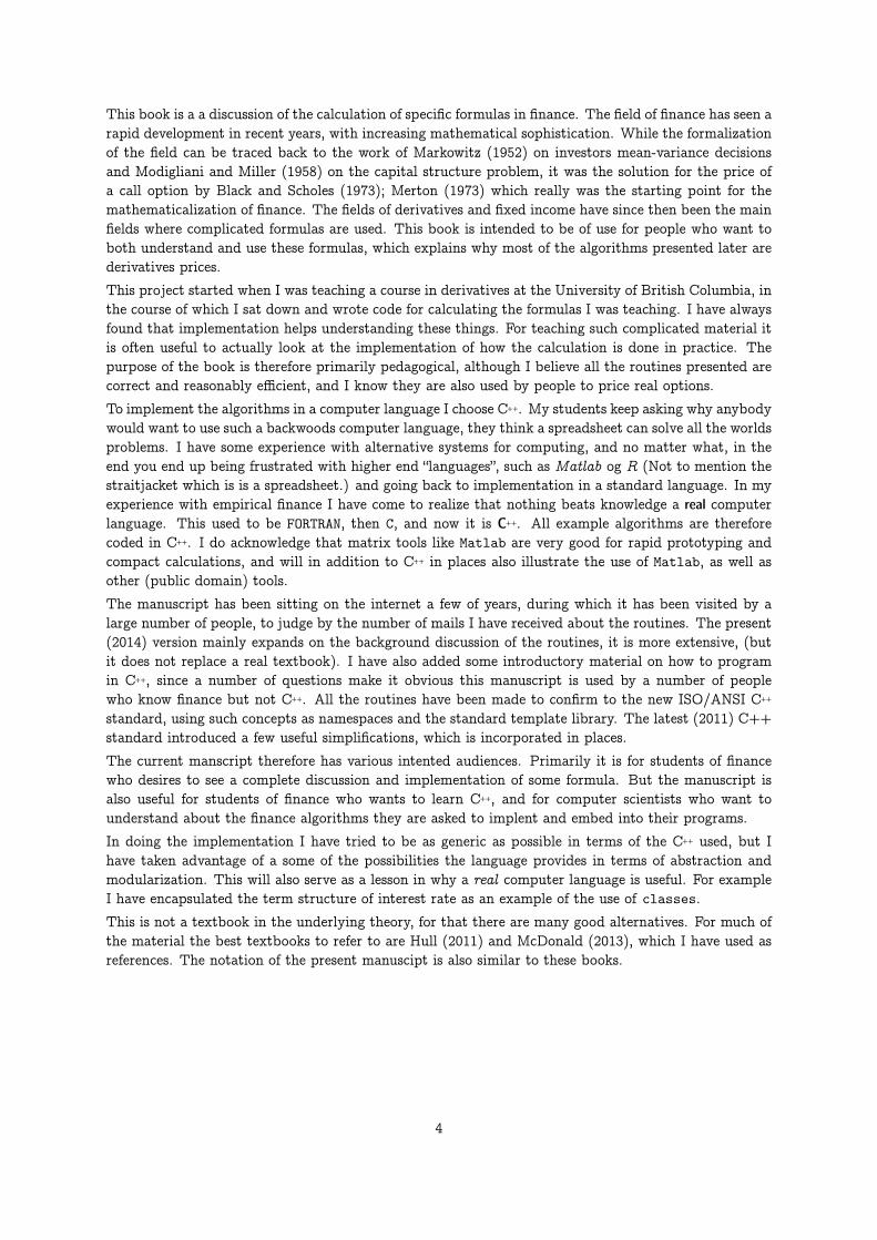
This book is a a discussion of the calculation of specific formulas in finance. The field of finance has seen arapid development in recent years, with increasing mathematical sophistication. While the formalizationof the field can be traced back to the work of Markowitz (1952) on investors mean-variance decisionsand Modigliani and Miller (1958) on the capital structure problem, it was the solution for the price ofa call option by Black and Scholes (1973); Merton (1973) which really was the starting point for themathematicalization of finance. The fields of derivatives and fixed income have since then been the mainfields where complicated formulas are used. This book is intended to be of use for people who want toboth understand and use these formulas, which explains why most of the algorithms presented later arederivatives prices.
This project started when I was teaching a course in derivatives at the University of British Columbia, inthe course of which I sat down and wrote code for calculating the formulas I was teaching. I have alwaysfound that implementation helps understanding these things. For teaching such complicated material itis often useful to actually look at the implementation of how the calculation is done in practice. Thepurpose of the book is therefore primarily pedagogical, although I believe all the routines presented arecorrect and reasonably efficient, and I know they are also used by people to price real options.
To implement the algorithms in a computer language I choose C++. My students keep asking why anybodywould want to use such a backwoods computer language, they think a spreadsheet can solve all the worldsproblems. I have some experience with alternative systems for computing, and no matter what, in theend you end up being frustrated with higher end “languages”, such as Matlab og R (Not to mention thestraitjacket which is is a spreadsheet.) and going back to implementation in a standard language. In myexperience with empirical finance I have come to realize that nothing beats knowledge a real computerlanguage. This used to be FORTRAN, then C, and now it is C++. All example algorithms are thereforecoded in C++. I do acknowledge that matrix tools like Matlab are very good for rapid prototyping andcompact calculations, and will in addition to C++ in places also illustrate the use of Matlab, as well asother (public domain) tools.
The manuscript has been sitting on the internet a few of years, during which it has been visited by alarge number of people, to judge by the number of mails I have received about the routines. The present(2014) version mainly expands on the background discussion of the routines, it is more extensive, (butit does not replace a real textbook). I have also added some introductory material on how to programin C++, since a number of questions make it obvious this manuscript is used by a number of peoplewho know finance but not C++. All the routines have been made to confirm to the new ISO/ANSI C++
standard, using such concepts as namespaces and the standard template library. The latest (2011) C++standard introduced a few useful simplifications, which is incorporated in places.
The current manscript therefore has various intented audiences. Primarily it is for students of financewho desires to see a complete discussion and implementation of some formula. But the manuscript isalso useful for students of finance who wants to learn C++, and for computer scientists who want tounderstand about the finance algorithms they are asked to implent and embed into their programs.
In doing the implementation I have tried to be as generic as possible in terms of the C++ used, but Ihave taken advantage of a some of the possibilities the language provides in terms of abstraction andmodularization. This will also serve as a lesson in why a real computer language is useful. For exampleI have encapsulated the term structure of interest rate as an example of the use of classes.
This is not a textbook in the underlying theory, for that there are many good alternatives. For much ofthe material the best textbooks to refer to are Hull (2011) and McDonald (2013), which I have used asreferences. The notation of the present manuscipt is also similar to these books.
4

Chapter 1
On C++ and programming.
Contents1.1 Compiling and linking . . . . . . . . . . . . . . . . . . . . . . . . . . . . . . . . . . . . . . . 51.2 The structure of a C++ program . . . . . . . . . . . . . . . . . . . . . . . . . . . . . . . . . 6
1.2.1 Types . . . . . . . . . . . . . . . . . . . . . . . . . . . . . . . . . . . . . . . . . 61.2.2 Operations . . . . . . . . . . . . . . . . . . . . . . . . . . . . . . . . . . . . . . 61.2.3 Functions and libraries . . . . . . . . . . . . . . . . . . . . . . . . . . . . . . . . 71.2.4 Templates and libraries . . . . . . . . . . . . . . . . . . . . . . . . . . . . . . . 71.2.5 Flow control . . . . . . . . . . . . . . . . . . . . . . . . . . . . . . . . . . . . . 81.2.6 Input Output . . . . . . . . . . . . . . . . . . . . . . . . . . . . . . . . . . . . . 81.2.7 Splitting up a program . . . . . . . . . . . . . . . . . . . . . . . . . . . . . . . . 81.2.8 Namespaces . . . . . . . . . . . . . . . . . . . . . . . . . . . . . . . . . . . . . . 9
1.3 Extending the language, the class concept. . . . . . . . . . . . . . . . . . . . . . . . . . . . 91.3.1 date, an example class . . . . . . . . . . . . . . . . . . . . . . . . . . . . . . . . 10
1.4 Const references . . . . . . . . . . . . . . . . . . . . . . . . . . . . . . . . . . . . . . . . . 161.5 Other C++ concepts . . . . . . . . . . . . . . . . . . . . . . . . . . . . . . . . . . . . . . . . 16
In this chapter I introduce C++ and discuss how to run programs written in C++. This is by no meansa complete reference to programming in C++, it is designed to give enough information to understandthe rest of the book. This chapter also only discusses a subset of C++, it concentrates on the parts ofthe language used in the remainder of this book. For really learning C++ a textbook is necessary. I havefound Lippman and Lajoie (1998) an excellent introduction to the language.1 The authorative sourceon the language is Stroustrup (1997b).
1.1 Compiling and linking
To program in C++ one has to first write a separate file with the program, which is then compiledinto low-level instructions (machine language) and linked with libraries to make a complete executableprogram. The mechanics of doing the compiling and linking varies from system to system, and we leavethese details as an exercise to the reader.
1I learned C++ from the previous edition of the book, Lippman (1992). From what I can tell the present editions stillseems like a good way of learning the language, but C++ has changed a lot in recent years.
5

1.2 The structure of a C++ program
The first thing to realize about C++ is that it is a strongly typed language. Everything must be declaredbefore it is used, both variables and functions. C++ has a few basic building blocks, which can be groupedinto types, operations and functions.
1.2.1 Types
The types we will work with in this book are bool, int, long, double and string.
Here are some example definitions
bool this_is_true=true;int i = 0;long j = 123456789;double pi = 3.141592653589793238462643;string s("this is a string");
The most important part of C++ comes from the fact that these basic types can be expanded by use ofclasses, of which more later.
1.2.2 Operations
To these basic types the common mathematical operations can be applied, such as addition, subtraction,multiplication and division:
int i = 100 + 50;int j = 100 - 50;int n = 100 * 2;int m = 100 / 2;
These operations are defined for all the common datatypes, with exception of the string type. Suchoperations can be defined by the programmer for other datatypes as well.
Increment and decrement In addition to these basic operations there are some additional operations withtheir own shorthand. An example we will be using often is incrementing and decrementing a variable.When we want to increase the value of one item by one, in most languages this is written:
int i=0;i = i+1;i = i-1;
In C++ this operation has its own shorthand
int i=0;i++;i--;
While this does not seem intuitive, and it is excusable to think that this operation is not really necessary,it does come in handy for more abstract data constructs. For example, as we will see later, if one definesa date class with the necessary operations, to get the next date will simply be a matter of
date d(1,1,1995);d++;
These two statements will result in the date in d being 2jan95.
6
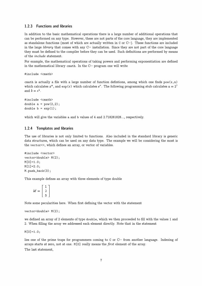
1.2.3 Functions and libraries
In addition to the basic mathematical operations there is a large number of additional operations thatcan be performed on any type. However, these are not parts of the core language, they are implementedas standalone functions (most of which are actually written in C or C++). These functions are includedin the large library that comes with any C++ installation. Since they are not part of the core languagethey must be defined to the compiler before they can be used. Such definitions are performed by meansof the include statement.
For example, the mathematical operations of taking powers and performing exponentiation are definedin the mathematical library cmath. In the C++ program one will write
#include <cmath>
cmath is actually a file with a large number of function defintions, among which one finds pow(x,n)which calculates xn, and exp(r) which calculates er. The following programming stub calculates a = 22
and b = e1.
#include <cmath>double a = pow(2,2);double b = exp(1);
which will give the variables a and b values of 4 and 2.718281828..., respectively.
1.2.4 Templates and libraries
The use of libraries is not only limited to functions. Also included in the standard library is genericdata structures, which can be used on any data type. The example we will be considering the most isthe vector<>, which defines an array, or vector of variables.
#include <vector>vector<double> M(2);M[0]=1.0;M[1]=2.0;M.push_back(3);
This example defines an array with three elements of type double
M =
24 1
2
3
35Note some pecularities here. When first defining the vector with the statement
vector<double> M(2);
we defined an array of 2 elements of type double, which we then proceeded to fill with the values 1 and2. When filling the array we addressed each element directly. Note that in the statement
M[0]=1.0;
lies one of the prime traps for programmers coming to C or C++ from another language. Indexing ofarrays starts at zero, not at one. M[0] really means the first element of the array.
The last statement,
7

M.push_back(3);
shows the ability of the programmer of changing the size of the array after it has been defined. push_backis a standard operation on arrays which “pushes” the element onto the back of the array, extending thesize of the array by one element. Most programming languages do not allow the programmer to specifyvariable-sized arrays “on the fly.” In FORTRAN or Pascal we would usually have to set a maximum lengthfor each array, and hope that we would not need to exceed that length. The vector<> template of C++
gets rid of the programmers need for “bookkeeping” in such array manipulations.
1.2.5 Flow control
To repeat statements several times one will use on of the possibilities for flow control, such as the foror while constucts. For example, to repeat an operation n times one can use the following for loop:
for (int i=0; i<n; i++) {some_operation(i);
};
The for statement has tree parts. The first part gives the initial condition (i=0). The next part theterminal condition (i<n), which says to stop when i<n is not fulfilled, which is at the n’th iteration.The last part is the increment statement (i++), saying what to do in each iteration. In this case thevalue of i is increased by one in each iteration. This is the typical for statement. One of the causesof C’s reputation for terseness is the possibility of elaborate for constructs, which end up being almostimpossible to read. In the algorithms presented in this book we will try to avoid any obfuscated forstatements, and stick to the basic cases.
1.2.6 Input Output
For any program to do anything useful it needs to be able to output its results. Input and outputoperations is defined in a couple of libraries, iostream and fstream. The first covers in/output tostandard terminals and the second in/output to files.
To write to standard output cout (the terminal), one will do as follows:
#include <iostream>cout << "This is a test" << endl;
To write to a file "test.out", one will do as follows:
#include <fstream>ofstream outf;outf.open("test.out");outf << "This is a test" << endl;outf.clear();outf.close();
1.2.7 Splitting up a program
Any nontrivial program in C++ is split into several pieces. Usually each piece is written as a functionwhich returns a value of a given type. To illustrate we provide a complete example program, shown inC++ Code 1.1.
8
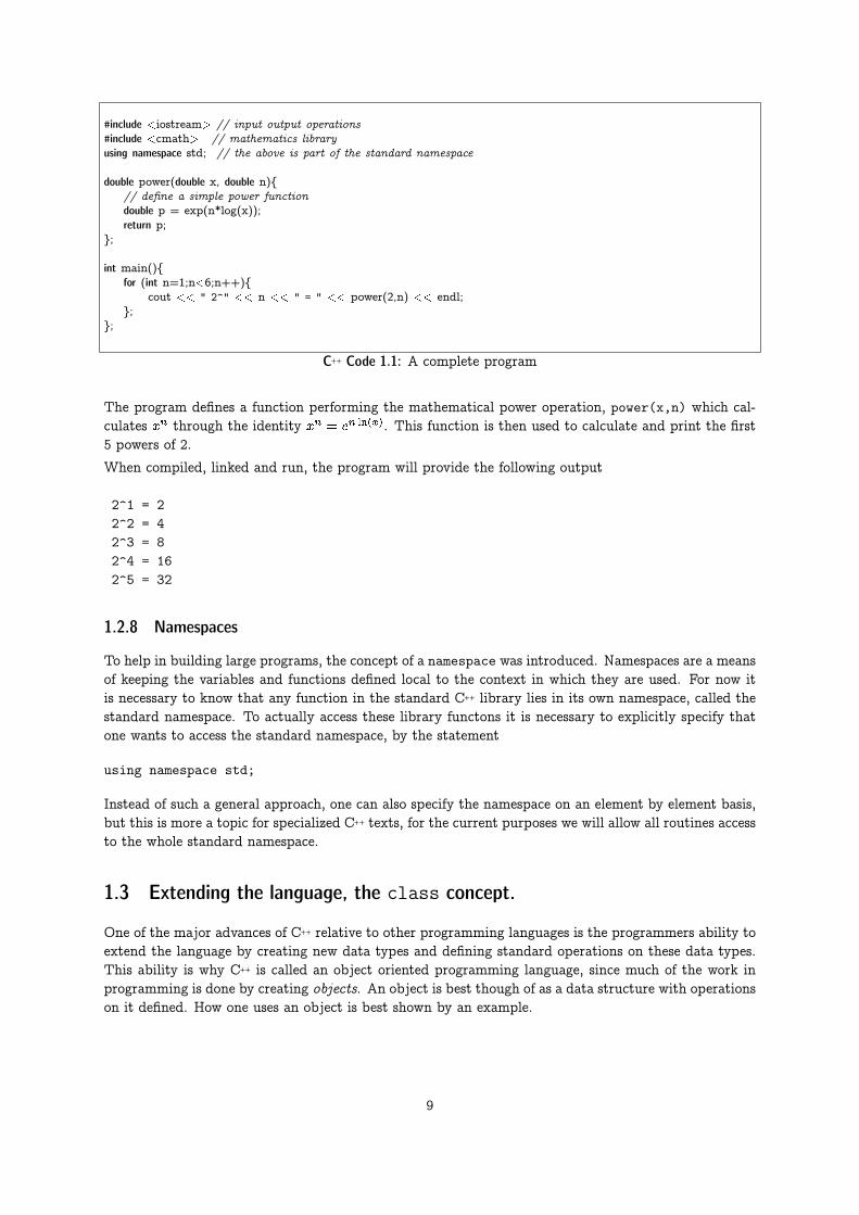
#include <iostream> // input output operations#include <cmath> // mathematics libraryusing namespace std; // the above is part of the standard namespace
double power(double x, double n){// define a simple power functiondouble p = exp(n*log(x));return p;
};
int main(){for (int n=1;n<6;n++){
cout << " 2^" << n << " = " << power(2,n) << endl;};
};
C++ Code 1.1: A complete program
The program defines a function performing the mathematical power operation, power(x,n) which cal-culates xn through the identity xn = en ln(x). This function is then used to calculate and print the first5 powers of 2.
When compiled, linked and run, the program will provide the following output
2^1 = 22^2 = 42^3 = 82^4 = 162^5 = 32
1.2.8 Namespaces
To help in building large programs, the concept of a namespace was introduced. Namespaces are a meansof keeping the variables and functions defined local to the context in which they are used. For now itis necessary to know that any function in the standard C++ library lies in its own namespace, called thestandard namespace. To actually access these library functons it is necessary to explicitly specify thatone wants to access the standard namespace, by the statement
using namespace std;
Instead of such a general approach, one can also specify the namespace on an element by element basis,but this is more a topic for specialized C++ texts, for the current purposes we will allow all routines accessto the whole standard namespace.
1.3 Extending the language, the class concept.
One of the major advances of C++ relative to other programming languages is the programmers ability toextend the language by creating new data types and defining standard operations on these data types.This ability is why C++ is called an object oriented programming language, since much of the work inprogramming is done by creating objects. An object is best though of as a data structure with operationson it defined. How one uses an object is best shown by an example.
9

1.3.1 date, an example class
Consider the abstract concept of a date. A date can be specified in any number of ways. Let us limitourselves to the Gregorian calendar. 12 august 2003 is a common way of specifying a date. However, itcan also be represented by the strings: “2003/8/12”, “12/8/2003” and so on, or by the number of yearssince 1 january 1900, the number of months since January, and the day of the month (which is how aUNIX programmer will think of it).
However, for most people writing programs the representation of a date is not relevant, they want to beable to enter dates in some abstract way, and then are conserned with such questions as:
� Are two dates equal?
� Is one date earlier than another?
� How many days is it between two dates?
A C++ programmer will proceed to use a class that embodies these uses of the concept of a date. Typicallyone will look around for an extant class which has already implemented this, but we will show a trivialsuch date class as an example of how one can create a class.
class date {protected:
int year ;int month ;int day ;
public:date();date(const int& d, const int& m, const int& y);
bool valid() const;
int day() const;int month() const;int year() const;
void set day (const int& day );void set month (const int& month );void set year (const int& year );
date operator ++(); // prefixdate operator ++(int); // postfixdate operator ��(); // prefixdate operator ��(int); // postfix
};
bool operator == (const date&, const date&); // comparison operatorsbool operator != (const date&, const date&);bool operator < (const date&, const date&);bool operator > (const date&, const date&);bool operator <= (const date&, const date&);bool operator >= (const date&, const date&);
Header file 1.1: Defining a date class
A class is defined in a header file, as shown in Header file 1.1. As internal representation of the date ischosen the three integers day_, month_ and year_. This is the data structure which is then manipulatedby the various functions defined below.
The functions are used to
10

� Create a date variable: date(const int& d, const int& m, const int& y);
� Functions outputting the date by the three integer functions day(), month() and year().
� Functions setting the date set_day(int), set_month(int) and set_year(int), which are usedby providing an integer as arguments to the function.
� Increment and decrement functions ++ and –
� Comparison functions <, <=, >, >=, == and !-.
After including this header file, programmers using such a class will then treat an object of type datejust like any other.
For exmple,
date d(1,1,2001);++d;
would result in the date object d containing the date 2 january 2001.
Any C++ programmer who want to use this date object will only need to look at the header file to knowwhat are the possible functions one can use with a date object, and be happy about not needing to knowanything about how these functions are implemented. This is the encapsulation part of object orientedprogramming, all relevant information about the date object is specified by the header file. This is theonly point of interaction, all details about implementation of the class objects and its functions is notused in code using this object. In fact, the user of the class can safely ignore the class’ privates, whichis only good manners, anyway.
Let us look at the implementation of this.
C++ Code 1.2 defines the basic operations, initialization, setting the date, and checking whether a date isvalid.
11

#include "date.h"
date::date(){ year = 0; month = 0; day = 0;};
date::date(const int& day, const int& month, const int& year){day = day;month = month;year = year;
};
int date::day() const { return day ; };int date::month() const { return month ; };int date::year() const { return year ; };
void date::set day (const int& day) { date::day = day; };void date::set month(const int& month) { date::month = month; };void date::set year (const int& year) { date::year = year; };
bool date::valid() const {// This function will check the given date is valid or not.// If the date is not valid then it will return the value false.// Need some more checks on the year, though
if (year <0) return false;if (month >12 j j month <1) return false;if (day >31 j j day <1) return false;if ((day ==31 && ( month ==2 j j month ==4 j j month ==6 j j month ==9 j j month ==11) ) )
return false;if ( day ==30 && month ==2) return false;// should also check for leap years, but for now allow for feb 29 in any yearreturn true;
};
C++ Code 1.2: Basic operations for the date class
12

For many abstract types it can be possible to define an ordering. For dates there is the natural ordering.C++ Code 1.3 shows how such comparison operations is defined.
#include "date.h"
bool operator == (const date& d1,const date& d2){ // check for equalityif (! (d1.valid() && (d2.valid())) ) { return false; }; /* if dates not valid, not clear what to do.
alternative: throw exception */return ((d1.day()==d2.day()) && (d1.month()==d2.month()) && (d1.year()==d2.year()));
};
bool operator < (const date& d1, const date& d2){if (! (d1.valid() && (d2.valid())) ) { return false; }; // see above remarkif (d1.year()==d2.year()) { // same year
if (d1.month()==d2.month()) { // same monthreturn (d1.day()<d2.day());
}else {
return (d1.month()<d2.month());};
}else { // different year
return (d1.year()<d2.year());};
};
// remaining operators defined in terms of the above
bool operator <=(const date& d1, const date& d2){if (d1==d2) { return true; }return (d1<d2);
}
bool operator >=(const date& d1, const date& d2) {if (d1==d2) { return true;};return (d1>d2);
};
bool operator > (const date& d1, const date& d2) { return !(d1<=d2);};
bool operator !=(const date& d1, const date& d2){ return !(d1==d2);}
C++ Code 1.3: Comparison operators for the date class
13

C++ Code 1.4 shows operations for finding previous and next date, called an iteration operator.
#include "date.h"
date next date(const date& d){if (!d.valid()) { return date(); }; //date ndat=date((d.day()+1),d.month(),d.year()); // first try adding a dayif (ndat.valid()) return ndat;ndat=date(1,(d.month()+1),d.year()); // then try adding a monthif (ndat.valid()) return ndat;ndat = date(1,1,(d.year()+1)); // must be next yearreturn ndat;
}
date previous date(const date& d){if (!d.valid()) { return date(); }; // return the default datedate pdat = date((d.day()�1),d.month(),d.year()); if (pdat.valid()) return pdat; // try same monthpdat = date(31,(d.month()�1),d.year()); if (pdat.valid()) return pdat; // try previous monthpdat = date(30,(d.month()�1),d.year()); if (pdat.valid()) return pdat;pdat = date(29,(d.month()�1),d.year()); if (pdat.valid()) return pdat;pdat = date(28,(d.month()�1),d.year()); if (pdat.valid()) return pdat;pdat = date(31,12,(d.year()�1)); // try previous yearreturn pdat;
};
date date::operator ++(int){ // postfix operatordate d = *this;*this = next date(d);return d;
}
date date::operator ++(){ // prefix operator*this = next date(*this);return *this;
}
date date::operator ��(int){ // postfix operator, return current valuedate d = *this;*this = previous date(*this);return d;
}
date date::operator ��(){ // prefix operator, return new value*this = previous date(*this);return *this;
};
C++ Code 1.4: Iterative operators for the date class
14
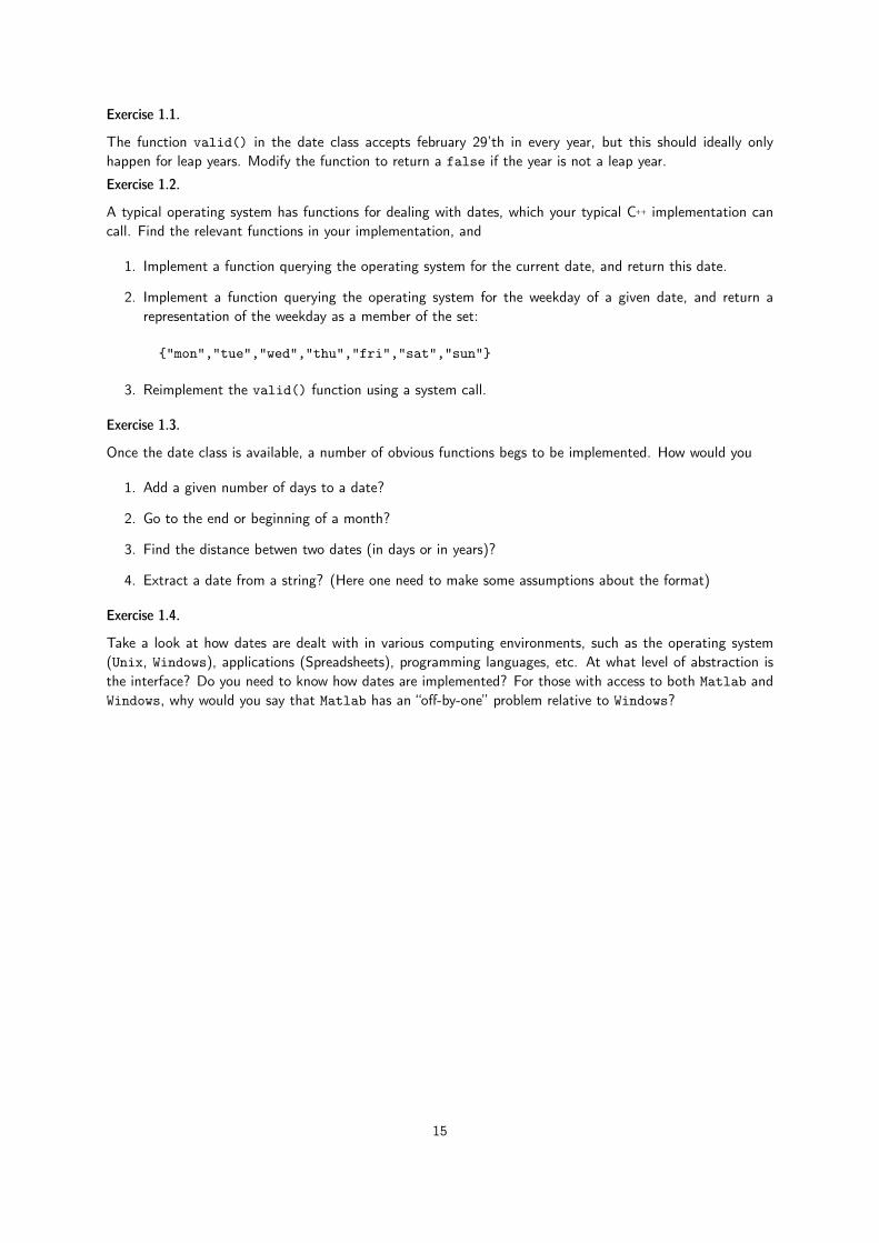
Exercise 1.1.
The function valid() in the date class accepts february 29’th in every year, but this should ideally onlyhappen for leap years. Modify the function to return a false if the year is not a leap year.
Exercise 1.2.
A typical operating system has functions for dealing with dates, which your typical C++ implementation cancall. Find the relevant functions in your implementation, and
1. Implement a function querying the operating system for the current date, and return this date.
2. Implement a function querying the operating system for the weekday of a given date, and return arepresentation of the weekday as a member of the set:
{"mon","tue","wed","thu","fri","sat","sun"}
3. Reimplement the valid() function using a system call.
Exercise 1.3.
Once the date class is available, a number of obvious functions begs to be implemented. How would you
1. Add a given number of days to a date?
2. Go to the end or beginning of a month?
3. Find the distance betwen two dates (in days or in years)?
4. Extract a date from a string? (Here one need to make some assumptions about the format)
Exercise 1.4.
Take a look at how dates are dealt with in various computing environments, such as the operating system(Unix, Windows), applications (Spreadsheets), programming languages, etc. At what level of abstraction isthe interface? Do you need to know how dates are implemented? For those with access to both Matlab andWindows, why would you say that Matlab has an “off-by-one” problem relative to Windows?
15

1.4 Const references
Let us now discuss a concept of more technical nature. Consider two alternative calls to a function,defined by function calls:
some_function(double r);some_function(const double& r);
They both are called by an argument which is a double, and that argument is guaranteed to not bechanged in the calling function, but they work differently. In the first case a copy of the variablereferenced to in the argument is created for use in the function, but in the second case one uses thesame variable, the argument is a reference to the location of the variable. The latter is more efficient,in particular when the argument is a large class. However, one worries that the variable referred to ischanged in the function, which in most cases one do not want. Therefore the const qualifier, it saysthat the function can not modify its argument. The compiler will warn the programmer if an attemptis made to modify such a variable.
For efficiency, in most of the following routines arguments are therefore given as as constant references.
1.5 Other C++ concepts
A number of other C++ concepts, such as function prototypes and templates, will be introduced later inparticular contexts. They only appear in a few places and is better introduced where they are used.
16

Chapter 2
Matrix Tools
Being computer literate entails being aware of a number of computer tools and being able to choose themost suitable tool for the problem at hand. Way to many people turns this around, and want to fitany problem to the computer tool they know. The tool that very often is the tool for business schoolstudents is a spreadsheet like Excel. Of course, a spreadsheet is very useful for very many businessapplications. However, it is not the best tool for more computationally intensive tasks.
While the bulk of the present book concerns itself with C++, in many applications in finance a veryhandy tool is a language for manipulating vectors and matrices using linear algebra. There are a lotof different possible programs that behaves very similarly, with a syntax taken from the mathematicalformulation of linear algebra. An early tool of this sort was matlab, with a large number of programscopying much of the syntax of this program. As a result of this there is a proliferation of programs withsimilar syntax to Matlab doing similar analysis. General tools include the commercial package Matlabsold by Mathworks, the public domain programs octave and scilab. Tools that are similar, but moregeared towards econometrics, include Gauss, Ox and S with its public domain “clone” R. As for whatprogram to install, there is no right answer. For the basic learning of how these tools work, any of thementioned packages will do the job. For students on a limited budget the public domain tools octave,scilab and R are obvious candidates. All of them perform the basic operations done by the commercialMatlab package, and good for learning the basics of such a matrix tool.
All of these tools are programs that lets the user manipulate vectors and matrices using very compactnotation. While compact notation is always prone to tense, making programs using it unreadable, thisis not such a large problem in Matlab, the notation tends to be so close how a mathematician wouldwrite them that programs can be relatively easy to follow. There are some pitfalls for the unwary user,in particular it is easy to “miss” the difference between a command operating on a whole matrix andthe corresponding element by element operation. For example, consider the following short example,where the operator ˆ means that the matrix A is taken to the power 2 (multiplied with itself), and theoperator .ˆ means that each element of the matrix A is taken to the power 2. The two commands givevery different answers.
>> A = [1 1 ; 1 1]A =1 11 1
>> A^2ans =2 22 2
>> A.^2ans =
17
1 11 1
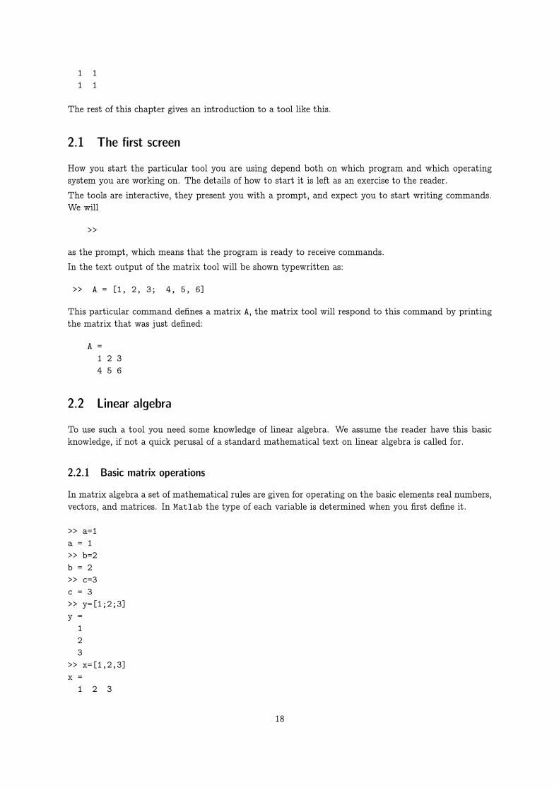
The rest of this chapter gives an introduction to a tool like this.
2.1 The first screen
How you start the particular tool you are using depend both on which program and which operatingsystem you are working on. The details of how to start it is left as an exercise to the reader.
The tools are interactive, they present you with a prompt, and expect you to start writing commands.We will
>>
as the prompt, which means that the program is ready to receive commands.
In the text output of the matrix tool will be shown typewritten as:
>> A = [1, 2, 3; 4, 5, 6]
This particular command defines a matrix A, the matrix tool will respond to this command by printingthe matrix that was just defined:
A =1 2 34 5 6
2.2 Linear algebra
To use such a tool you need some knowledge of linear algebra. We assume the reader have this basicknowledge, if not a quick perusal of a standard mathematical text on linear algebra is called for.
2.2.1 Basic matrix operations
In matrix algebra a set of mathematical rules are given for operating on the basic elements real numbers,vectors, and matrices. In Matlab the type of each variable is determined when you first define it.
>> a=1a = 1>> b=2b = 2>> c=3c = 3>> y=[1;2;3]y =123
>> x=[1,2,3]x =1 2 3
18

>> A=[1 2 3;4 5 6]A =1 2 34 5 6
Observe that when filling in a vector or a matrix a space or a comma means a new number, a semicolona new row. To suppress the printing of what you just defined, end the line with a semicolon:
>> A=[1,2,3,4];>> A=[1,2,3,4]A =1 2 3 4
>>
You can also use defined variables to define new variables, as long as the dimensions make sense. Forexample, given the above definitions:
>>B=[c x]B =3 1 2 3
>> C = [A;x]C =1 2 34 5 61 2 3
>> D = [A y]error: number of rows must matcherror: evaluating assignment expression near line 22, column 3
If the dimensioning is wrong, you get an error message, and the variable is not defined.
To see what is in a variable, tell Matlab to print the value by giving the name:
>> aa = 1>> AA =1 2 34 5 6
Note that Matlab is case-sensitive, both A and a are defined.
2.2.2 Arithmetic Matrix Operations.
We now get to the important parts of Matlab, namely, its built–in matrix arithmetic. Given the defi-nitions above, let us add and subract a few elements according to the rules of matrix algebra. We firstshow how to manipulate numbers and vectors:
>> a=1a = 1>> b=2b = 2>> a+bans = 3
19

>> x=[1 2 3 4]x =
1 2 3 4>> y=[4 3 2 1]y =
4 3 2 1>> x+yans =
5 5 5 5>> y-xans =
3 1 -1 -3>> a*x+b*yans =
9 8 7 6
similarly, for matrices:
A=[1 2 3; 4 5 6]A =
1 2 34 5 6
>> B=[6 5 4; 3 2 1]B =
6 5 43 2 1
>> A+Bans =
7 7 77 7 7
>>A-Bans =-5 -3 -11 3 5
>> a*A+b*Bans =
13 12 1110 9 8
> A*B’ans =
28 1073 28
In linear algebra, you need to be aware that matrix multiplication is not element by element multiplica-tion, it is a much more complex operation, where all possible vector combinations are multiplied witheach other. When multiplying matrices, you need to be more careful about dimensions, but in terms ofnotation it is just like vector multiplication.
>> A=[1 2 3;4 5 6]A =1 2 34 5 6
>> B = [1 2;3 4; 5 6]
20
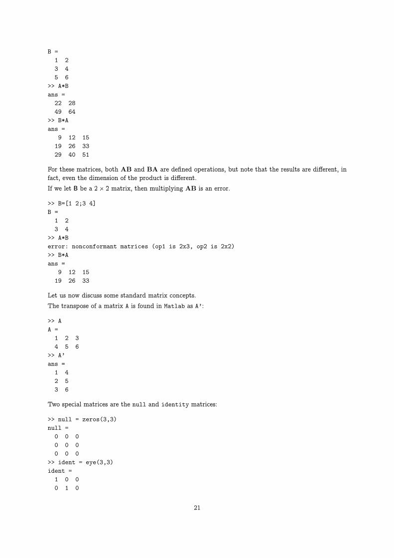
B =1 23 45 6
>> A*Bans =22 2849 64
>> B*Aans =
9 12 1519 26 3329 40 51
For these matrices, both AB and BA are defined operations, but note that the results are different, infact, even the dimension of the product is different.
If we let B be a 2� 2 matrix, then multiplying AB is an error.
>> B=[1 2;3 4]B =1 23 4
>> A*Berror: nonconformant matrices (op1 is 2x3, op2 is 2x2)>> B*Aans =
9 12 1519 26 33
Let us now discuss some standard matrix concepts.
The transpose of a matrix A is found in Matlab as A’:
>> AA =1 2 34 5 6
>> A’ans =1 42 53 6
Two special matrices are the null and identity matrices:
>> null = zeros(3,3)null =0 0 00 0 00 0 0
>> ident = eye(3,3)ident =1 0 00 1 0
21

0 0 1
The rank of a matrix is is the number of independent rows or columns in the matrix, and calculated as
>> AhiA =1 2 34 5 6
>> rank(A)ans = 2
The inverse of a square matrix A is the matrix inv(A) such that A*inv(A) equals the identity matrix,or in mathematical notation AA�1 = I.
>> D=[1 2;1 4]D =
1 21 4
>> inv(D)ans =
2.00000 -1.00000-0.50000 0.50000
>> D^-1ans =
2.00000 -1.00000-0.50000 0.50000
To make sure that this is the inverse, multiply D and inv(D):
>> D * inv(D)ans =1 00 1
Determinant
>> BB =1 23 4
>> det(B)ans = -2
2.3 Solving linear equations
Consider the basic linear equation
Ax = b
This equation has a defined solution if the rank of A equals the rank of [Ajb]. If A is nonsingular, wesolve the linear equation by finding the unique solution
x = A�1b
22

Consider the linear equation
3x1 + 4x2 = 5
4x1 + 6x2 = 8
Write this in matrix form by defining
A =
�3 4
4 6
�
b =
�5
8
�Let us first check that this system is solvable
>> A = [3 4;4 6]A =3 44 6
>> b=[5;8]b =
58
>> rank(A)ans = 2>> rank ([A b])ans = 2
Note how to create the augmented matrix [Ajb] by [A b]. The rank of the two is the same. Since A issquare, we can calculate the solution as
>> inverse(A)ans =
3.0000 -2.0000-2.0000 1.5000
>> x = inverse(A) * bx =-12
The solution to the system of equations is
x =
� �12
�In this case we calculated the solution by finding the inverse. But you should be aware that solvingthe system of equations by calculation of the inverse is not the numerically most stable way of doingthe calculation. Matlab has built in a direct linear matrix solver, which is invoked by the left divisionoperator
>> x = A\bx =-12
23
This solves the system of equations directly, and it is usually the preferred way to do this operation,unless the inverse is needed for other purposes.
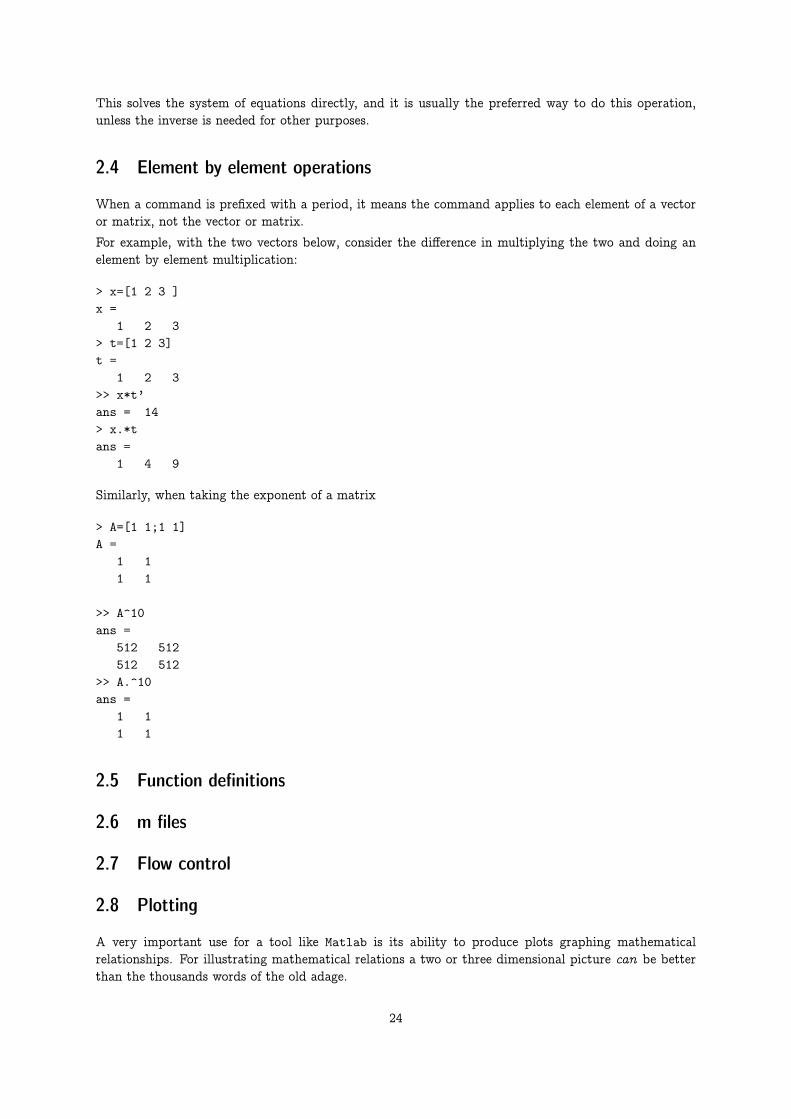
2.4 Element by element operations
When a command is prefixed with a period, it means the command applies to each element of a vectoror matrix, not the vector or matrix.
For example, with the two vectors below, consider the difference in multiplying the two and doing anelement by element multiplication:
> x=[1 2 3 ]x =
1 2 3> t=[1 2 3]t =
1 2 3>> x*t’ans = 14> x.*tans =
1 4 9
Similarly, when taking the exponent of a matrix
> A=[1 1;1 1]A =
1 11 1
>> A^10ans =
512 512512 512
>> A.^10ans =
1 11 1
2.5 Function definitions
2.6 m files
2.7 Flow control
2.8 Plotting
A very important use for a tool like Matlab is its ability to produce plots graphing mathematicalrelationships. For illustrating mathematical relations a two or three dimensional picture can be betterthan the thousands words of the old adage.
24

2.9 Libraries
2.10 References
You need the manual for your chosen package.
25

Chapter 3
The value of time
Contents3.1 Present value . . . . . . . . . . . . . . . . . . . . . . . . . . . . . . . . . . . . . . . . . . . 263.2 One interest rate with annual compounding . . . . . . . . . . . . . . . . . . . . . . . . . . . . 27
3.2.1 Internal rate of return. . . . . . . . . . . . . . . . . . . . . . . . . . . . . . . . . 303.3 Continously compounded interest . . . . . . . . . . . . . . . . . . . . . . . . . . . . . . . . . 34
3.3.1 Present value . . . . . . . . . . . . . . . . . . . . . . . . . . . . . . . . . . . . . 353.4 Further readings . . . . . . . . . . . . . . . . . . . . . . . . . . . . . . . . . . . . . . . . . . 35
Finance as a field of study is sometimes somewhat flippantly said to deal with the value of two things:time and risk. While this is not the whole story, there is a deal of truth in it. These are the two issueswhich is always present. We start our discussion by ignoring risk and only considering the implicationsof the fact that anybody prefers to get something earlier rather than later, or the value of time.
3.1 Present value
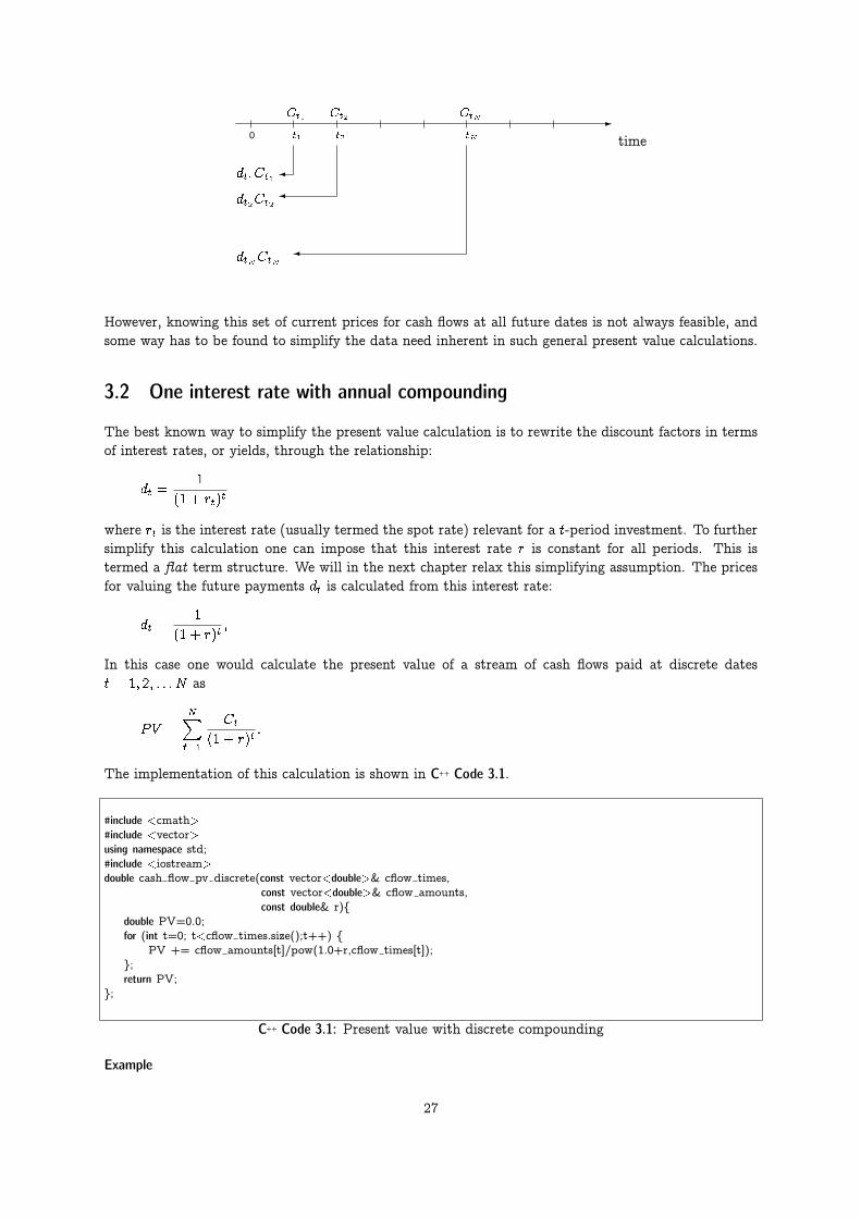
The present value is the current value of a stream of future payments. Let Ct be the cash flow at timet. Suppose we have N future cash flows that occur at times t1; t2; � � � ; tN .
-0 t1 t2 tN
C1 C2 CN
time
To find the present value of these future cash flows one need a set of prices of future cash flows. Supposedt is the price one would pay today for the right to receive one dollar at a future date t. Such a priceis also called a discount factor. To complicate matters further such prices will differ depending on theriskiness of the future cash flows. For now we concentrate on one particular set of prices, the prices ofriskless future cash flows. We will return to how one would adjust the prices for risky cash flows.
If one knows the set of prices for future claims of one dollar, d1; d2; : : : ;, one would calculate the presentvalue as the sum of the present values of the different elements.
PV =
NXi=1
dtiCti
26
-0 t1 t2 tN
Ct1 Ct2 CtN
time
�dt1Ct1
�dt2Ct2
�dtNCtN
However, knowing this set of current prices for cash flows at all future dates is not always feasible, andsome way has to be found to simplify the data need inherent in such general present value calculations.
3.2 One interest rate with annual compounding
The best known way to simplify the present value calculation is to rewrite the discount factors in termsof interest rates, or yields, through the relationship:
dt =1
(1 + rt)t
where rt is the interest rate (usually termed the spot rate) relevant for a t-period investment. To furthersimplify this calculation one can impose that this interest rate r is constant for all periods. This istermed a flat term structure. We will in the next chapter relax this simplifying assumption. The pricesfor valuing the future payments dt is calculated from this interest rate:
dt =1
(1 + r)t;
In this case one would calculate the present value of a stream of cash flows paid at discrete datest = 1; 2; : : : N as
PV =
NXt=1
Ct
(1 + r)t:
The implementation of this calculation is shown in C++ Code 3.1.
#include <cmath>#include <vector>using namespace std;#include <iostream>double cash flow pv discrete(const vector<double>& cflow times,
const vector<double>& cflow amounts,const double& r){
double PV=0.0;for (int t=0; t<cflow times.size();t++) {
PV += cflow amounts[t]/pow(1.0+r,cflow times[t]);};return PV;
};
C++ Code 3.1: Present value with discrete compounding
Example
27
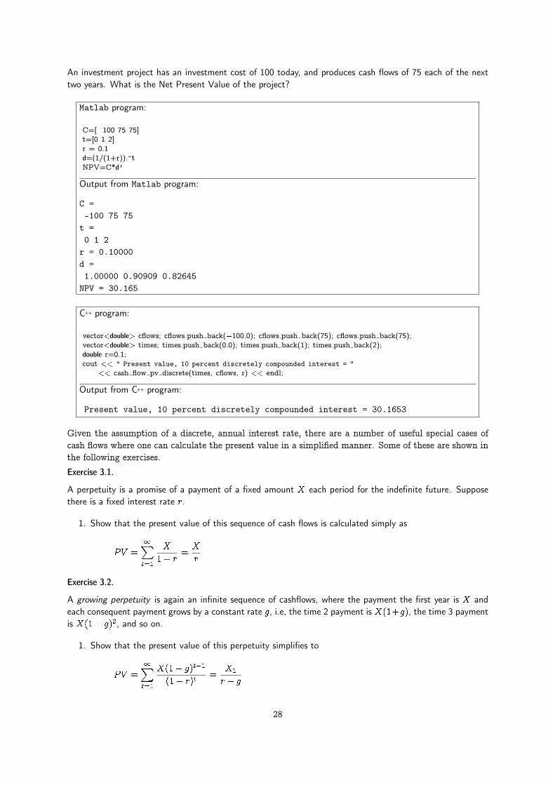
An investment project has an investment cost of 100 today, and produces cash flows of 75 each of the nexttwo years. What is the Net Present Value of the project?
Matlab program:
C=[�100 75 75]t=[0 1 2]r = 0.1d=(1/(1+r)).^tNPV=C*d’
Output from Matlab program:
C =-100 75 75t =0 1 2r = 0.10000d =1.00000 0.90909 0.82645NPV = 30.165
C++ program:
vector<double> cflows; cflows.push back(�100.0); cflows.push back(75); cflows.push back(75);vector<double> times; times.push back(0.0); times.push back(1); times.push back(2);double r=0.1;cout << " Present value, 10 percent discretely compounded interest = "
<< cash flow pv discrete(times, cflows, r) << endl;
Output from C++ program:
Present value, 10 percent discretely compounded interest = 30.1653
Given the assumption of a discrete, annual interest rate, there are a number of useful special cases ofcash flows where one can calculate the present value in a simplified manner. Some of these are shown inthe following exercises.
Exercise 3.1.
A perpetuity is a promise of a payment of a fixed amount X each period for the indefinite future. Supposethere is a fixed interest rate r.
1. Show that the present value of this sequence of cash flows is calculated simply as
PV =
1Xt=1
X
1 + r=X
r
Exercise 3.2.
A growing perpetuity is again an infinite sequence of cashflows, where the payment the first year is X andeach consequent payment grows by a constant rate g, i.e, the time 2 payment is X(1+g), the time 3 paymentis X(1 + g)2, and so on.
1. Show that the present value of this perpetuity simplifies to
PV =
1Xt=1
X(1 + g)t�1
(1 + r)t=
X1
r � g
28
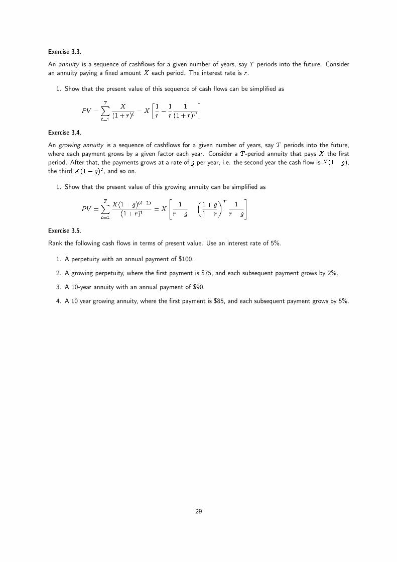
Exercise 3.3.
An annuity is a sequence of cashflows for a given number of years, say T periods into the future. Consideran annuity paying a fixed amount X each period. The interest rate is r.
1. Show that the present value of this sequence of cash flows can be simplified as
PV =
TXt=1
X
(1 + r)t= X
�1
r� 1
r
1
(1 + r)T
�
Exercise 3.4.
An growing annuity is a sequence of cashflows for a given number of years, say T periods into the future,where each payment grows by a given factor each year. Consider a T -period annuity that pays X the firstperiod. After that, the payments grows at a rate of g per year, i.e. the second year the cash flow is X(1+ g),the third X(1 + g)2, and so on.
1. Show that the present value of this growing annuity can be simplified as
PV =
TXt=1
X(1 + g)(t�1)
(1 + r)t= X
"1
r � g��1 + g
1 + r
�T1
r � g
#
Exercise 3.5.
Rank the following cash flows in terms of present value. Use an interest rate of 5%.
1. A perpetuity with an annual payment of $100.
2. A growing perpetuity, where the first payment is $75, and each subsequent payment grows by 2%.
3. A 10-year annuity with an annual payment of $90.
4. A 10 year growing annuity, where the first payment is $85, and each subsequent payment grows by 5%.
29

3.2.1 Internal rate of return.
In addition to its role in simplifying present value calculations, the interest rate has some further use.The percentage return on an investment is a summary measure of the investment’s profitability. Sayingthat an investment earns 10% per year is a good way of summarizing the cash flows in a way that does notdepend on the amount of the initial investment. The return is thus a relative measure of profitability.To estimate a return for a set of cash flows we calculate the internal rate of return. The internalrate of return for a set of cash flows is the interest rate that makes the present value of the cash flowsequal to zero. When there is a uniquely defined internal rate of return we get a relative measure of theprofitability of a set of cash flows, measured as a return, typically expressed as a percentage. Note someof the implicit assumptions made here. We assume that the same interest rate applies at all future dates(i.e. a flat term structure). The IRR method also assumes intermediate cash flows are reinvested at theinternal rate of return.
Suppose the cash flows are C0; C1; C2; : : : CT . Finding an internal rate of return is finding a solution y
of the equation
TXt=1
Ct
(1 + y)t� C0 = 0
Note that this is a polynomial equation, and as T becomes large, there in no way to find an explicitsolution to the equation. It therefore needs to be solved numerically. For well behaved cash flows, wherewe know that there is one IRR, the method implemented in C++ Code 3.2 is suitable, it is an iterativeprocess called bisection. It is an adaption of the bracketing approach discussed in (Press, Teukolsky,Vetterling, and Flannery, 1992, Chapter9),
30

#include <cmath>#include <algorithm>#include <vector>using namespace std;#include "fin_recipes.h"
const double ERROR=�1e30;
double cash flow irr discrete(const vector<double>& cflow times,const vector<double>& cflow amounts) {
// simple minded irr function. Will find one root (if it exists.)// adapted from routine in Numerical Recipes in C.if (cflow times.size()!=cflow amounts.size()) return ERROR;const double ACCURACY = 1.0e�5;const int MAX ITERATIONS = 50;double x1 = 0.0;double x2 = 0.2;
// create an initial bracket, with a root somewhere between bot,topdouble f1 = cash flow pv discrete(cflow times, cflow amounts, x1);double f2 = cash flow pv discrete(cflow times, cflow amounts, x2);int i;for (i=0;i<MAX ITERATIONS;i++) {
if ( (f1*f2) < 0.0) { break; }; //if (fabs(f1)<fabs(f2)) {
f1 = cash flow pv discrete(cflow times,cflow amounts, x1+=1.6*(x1�x2));}else {
f2 = cash flow pv discrete(cflow times,cflow amounts, x2+=1.6*(x2�x1));};
};if (f2*f1>0.0) { return ERROR; };double f = cash flow pv discrete(cflow times,cflow amounts, x1);double rtb;double dx=0;if (f<0.0) {
rtb = x1;dx=x2�x1;
}else {
rtb = x2;dx = x1�x2;
};for (i=0;i<MAX ITERATIONS;i++){
dx *= 0.5;double x mid = rtb+dx;double f mid = cash flow pv discrete(cflow times,cflow amounts, x mid);if (f mid<=0.0) { rtb = x mid; }if ( (fabs(f mid)<ACCURACY) j j (fabs(dx)<ACCURACY) ) return x mid;
};return ERROR; // error.
};
C++ Code 3.2: Estimation of the internal rate of return
31

Example
We are considering an investment with the following cash flows at dates 0, 1 and 2:
C0 = �100; C1 = 10; C2 = 110
1. The current interest rate (with discrete, annual compounding) is 5%. Determine the present value ofthe cash flows.
2. Find the internal rate of return of this sequence of cash flows.
Matlab program:
C=[�100 10 110]t=[0 1 2]r = 0.05d=(1/(1+r)).^tNPV=C*d’IRR = irr(C)
Output from Matlab program:
C =-100 10 110t =0 1 2r = 0.050000d =1.00000 0.95238 0.90703NPV = 9.2971IRR = 0.100000
C++ program:
vector<double> cflows; cflows.push back(�100.0); cflows.push back(10.0); cflows.push back(110.0);vector<double> times; times.push back(0.0); times.push back(1); times.push back(2);double r=0.05;cout << " present value, 5 percent discretely compounded interest = " ;cout << cash flow pv discrete(times, cflows, r) << endl;cout << " internal rate of return, discrete compounding = ";cout << cash flow irr discrete(times, cflows) << endl;
Output from C++ program:
present value, 5 percent discretely compounded interest = 9.29705internal rate of return, discrete compounding = 0.1
32

In addition to the above economic qualifications to interpretations of the internal rate of return, we alsohave to deal with technical problem stemming from the fact that any polynomial equation has potentiallyseveral solutions, some of which may be imaginary. By imaginary here we mean that we move away fromthe real line to the set of complex numbers. In economics we prefer the real solutions, complex interestrates are not something we have much intuition about... To see whether we are likely to have problemsin identifying a single meaningful IRR, the code shown in code 3.3 implements a simple check. It is onlya necessary condition for a unique IRR, not sufficient, so you may still have a well-defined IRR evenif this returns false. The first test is just to count the number of sign changes in the cash flow. FromDescartes rule we know that the number of real roots is one if there is only one sign change. If there ismore than one change in the sign of cash flows, we can go further and check the aggregated cash flowsfor sign changes (See Norstrom (1972)).
#include <cmath>#include <vector>using namespace std;
inline int sgn(const double& r){ if (r>=0) {return 1;} else {return �1;}; };
bool cash flow unique irr(const vector<double>& cflow times,const vector<double>& cflow amounts) {
int sign changes=0; // first check Descartes rulefor (int t=1;t<cflow times.size();++t){
if (sgn(cflow amounts[t�1]) !=sgn(cflow amounts[t])) sign changes++;};if (sign changes==0) return false; // can not find any irrif (sign changes==1) return true;
double A = cflow amounts[0]; // check the aggregate cash flows, due to Norstromsign changes=0;for (int t=1;t<cflow times.size();++t){
if (sgn(A) != sgn(A+=cflow amounts[t])) sign changes++;};if (sign changes<=1) return true;return false;
}
C++ Code 3.3: Test for uniqueness of IRR
A better way to gain an understanding for the relationship between the interest rate and the presentvalue is simply to plot the present value as a function of the interest rate. The following picture illustratesthe method for two different cash flows. Note that the set of cash flows on the right has two possbleinterest rates that sets the present value equal to zero.
-15
-10
-5
0
5
10
0 0.02 0.04 0.06 0.08 0.1 0.12
pv(r)0
-5
-4
-3
-2
-1
0
1
2
-0.2 -0.15 -0.1 -0.05 0 0.05 0.1 0.15 0.2
pv(r)0
C0 = �100; C1 = 10; C2 = 100 C0 = �100; C1 = 201; C2 = �100
33
Exercise 3.6.
An alternative way of estimating the IRR is to use an external subroutine that finds the root of a polynomialequation. Search for a suitable general subroutine for root finding and replace the IRR estimation with a callto this subroutine.
3.3 Continously compounded interest
Such discrete compounding as we have just discussed is not the only alternative way to approximate thediscount factor. The discretely compounded case assumes that interest is added at discrete points in time(hence the name). However, an alternative assumption is to assume that interest is added continously. Ifcompounding is continous, and r is the interest rate, one would calculate the current price dt of recivingone dollar at a future date t as
dt = e�rt;
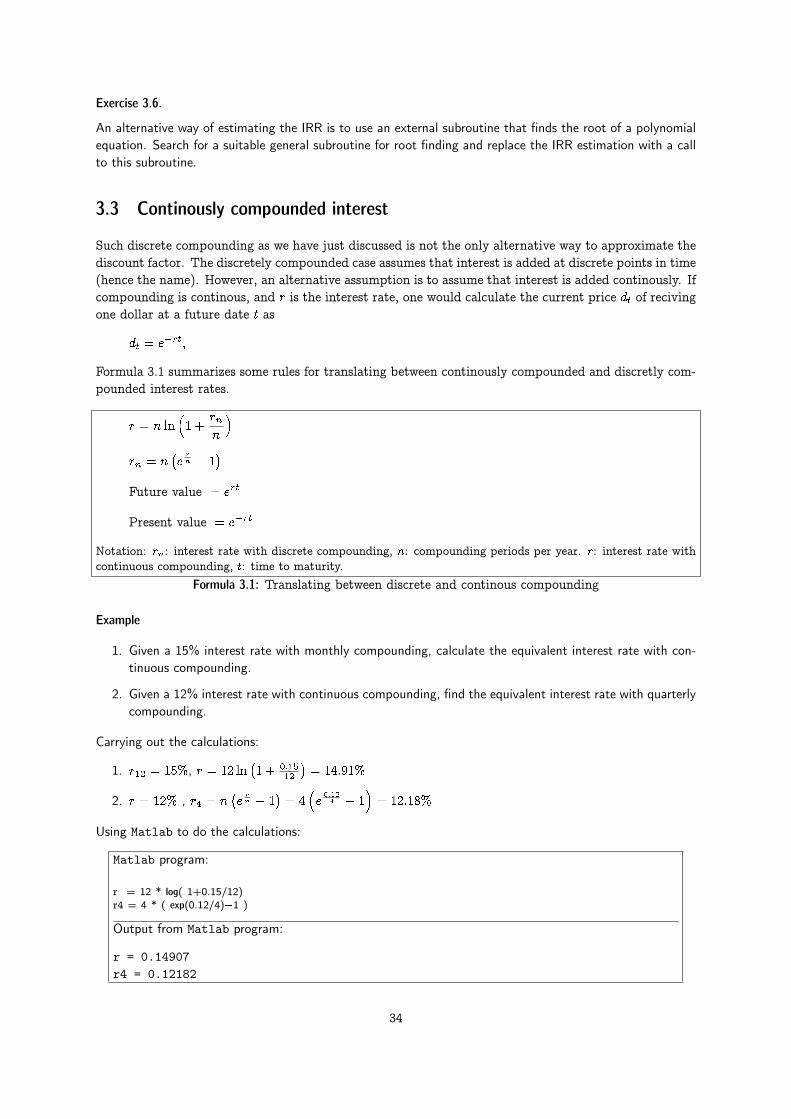
Formula 3.1 summarizes some rules for translating between continously compounded and discretly com-pounded interest rates.
r = n ln�1 +
rnn
�rn = n
�ern � 1
�Future value = ert
Present value = e�rt
Notation: rn: interest rate with discrete compounding, n: compounding periods per year. r: interest rate withcontinuous compounding, t: time to maturity.
Formula 3.1: Translating between discrete and continous compounding
Example
1. Given a 15% interest rate with monthly compounding, calculate the equivalent interest rate with con-tinuous compounding.
2. Given a 12% interest rate with continuous compounding, find the equivalent interest rate with quarterlycompounding.
Carrying out the calculations:
1. r12 = 15%, r = 12 ln�1 + 0:15
12
�= 14:91%
2. r = 12% , r4 = n�ern � 1
�= 4
�e0:124 � 1
�= 12:18%
Using Matlab to do the calculations:
Matlab program:
r = 12 * log( 1+0.15/12)r4 = 4 * ( exp(0.12/4)�1 )
Output from Matlab program:
r = 0.14907r4 = 0.12182
34
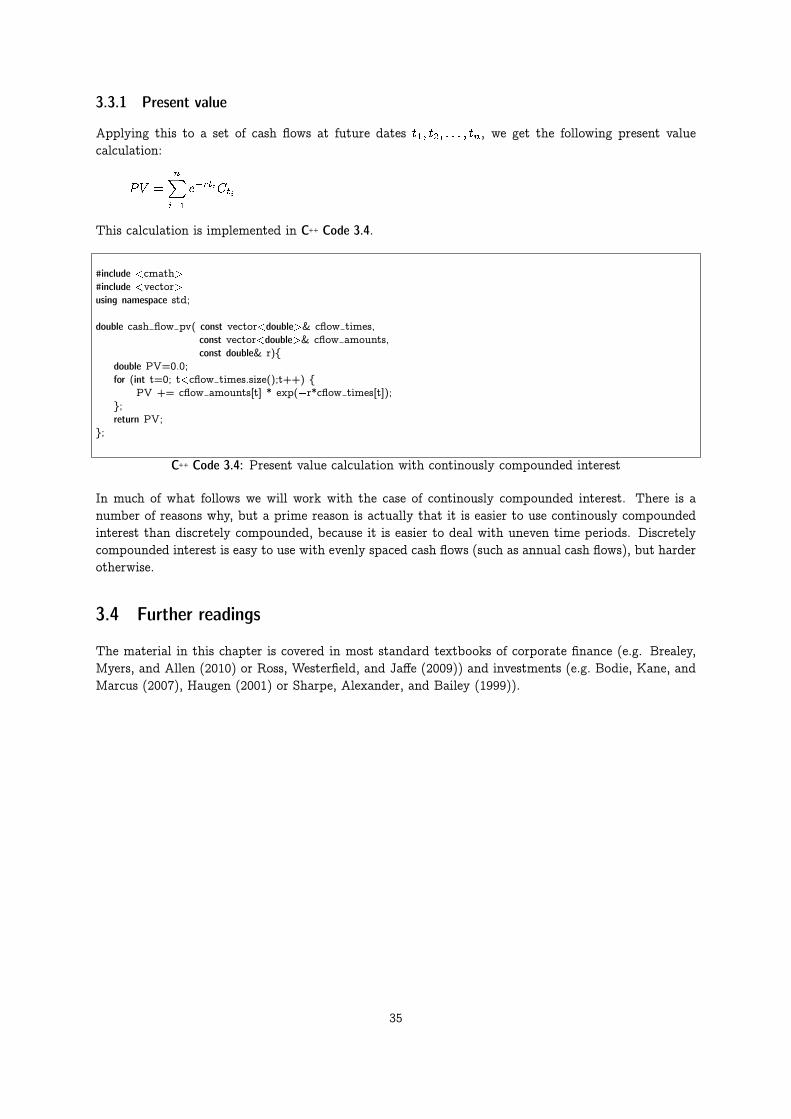
3.3.1 Present value
Applying this to a set of cash flows at future dates t1; t2; : : : ; tn, we get the following present valuecalculation:
PV =
nXi=1
e�rtiCti
This calculation is implemented in C++ Code 3.4.
#include <cmath>#include <vector>using namespace std;
double cash flow pv( const vector<double>& cflow times,const vector<double>& cflow amounts,const double& r){
double PV=0.0;for (int t=0; t<cflow times.size();t++) {
PV += cflow amounts[t] * exp(�r*cflow times[t]);};return PV;
};
C++ Code 3.4: Present value calculation with continously compounded interest
In much of what follows we will work with the case of continously compounded interest. There is anumber of reasons why, but a prime reason is actually that it is easier to use continously compoundedinterest than discretely compounded, because it is easier to deal with uneven time periods. Discretelycompounded interest is easy to use with evenly spaced cash flows (such as annual cash flows), but harderotherwise.
3.4 Further readings
The material in this chapter is covered in most standard textbooks of corporate finance (e.g. Brealey,Myers, and Allen (2010) or Ross, Westerfield, and Jaffe (2009)) and investments (e.g. Bodie, Kane, andMarcus (2007), Haugen (2001) or Sharpe, Alexander, and Bailey (1999)).
35

Chapter 4
Bond Pricing with a flat term structure
Contents4.1 Flat term structure with discrete, annual compounding . . . . . . . . . . . . . . . . . . . . . . 37
4.1.1 Bond Price . . . . . . . . . . . . . . . . . . . . . . . . . . . . . . . . . . . . . . 374.1.2 Yield to maturity . . . . . . . . . . . . . . . . . . . . . . . . . . . . . . . . . . . 384.1.3 Duration . . . . . . . . . . . . . . . . . . . . . . . . . . . . . . . . . . . . . . . 414.1.4 Measuring bond sensitivity to interest rate changes . . . . . . . . . . . . . . . . 43
4.2 Continously compounded interest . . . . . . . . . . . . . . . . . . . . . . . . . . . . . . . . . 474.3 Further readings . . . . . . . . . . . . . . . . . . . . . . . . . . . . . . . . . . . . . . . . . . 50
In this section we use the present value framework of the previous chapter to price bonds and other fixedincome securities. What distinguishes bonds is that the future payments are set when the security isissued. The simplest, and most typical bond, is a fixed interest, constant maturity bond with no defaultrisk. There is however a large number of alternative contractual features of bonds. The bond could forexample ba an annuity bond, paying a fixed amount each period. For such a bond the principal amountoutstanding is paid gradually during the life of the bond. The interest rate the bond pays need not befixed, it could be a floating rate, the interest rate paid could be a function of some market rate. Manybonds are issued by corporations, and in such cases there is a risk that the company issued the bonddefaults, and the bond does not pay the complete promised amount. Another thing that makes bondpricing difficult in practice, is that interest rates tend to change over time.
We start by assuming that all the promised payments are certain.
Then the bond current price B0 is found as the present value of these payments. The first step of pricingis to use the terms of the bond to find the promised payments. We start by considering a fixed interestbond with no default risk. Such bonds are typically bonds issued by governments. The bond is a promiseto pay a face value F at the maturity date T periods from now. Each period the bond pays a fixedpercentage amount of the face value as coupon C. The cash flows from the bond thus look as follows.
t = 0 1 2 3 � � � T
Coupon C C C � � � C
Face value F
Total cash flows C1 = C C2 = C � � � CT = C + F
In general a bond price is found as the present value
B0 = d1C1 + d2C2 + � � �+ dTCT =
TXt=1
dtCt
where dt is the discount factor, or the time 0 price of a payment of 1 at time t. To fully specify the
36

problem it is necessary to find all discount factors dt. In this chapter we will work with a specially simplespecifiction of the term structure, namely that it is flat, and specified by the interest rate r.
4.1 Flat term structure with discrete, annual compounding
This is the simplest possible specification of a term structure,
dt =
�1
1 + r
�t=
1
(1 + r)t
4.1.1 Bond Price
The current bond price (B0) is the present value of the cash flows from the bond
B0 =
TXt=1
�1
(1 + r)t
�Ct =
TXt=1
Ct
(1 + r)t(4.1)
If we continue with the example of a standard fixed interest bond, where Ct = C when t < T andCT = C + F , and show how the bond price will be calculated using Matlab.
Example
A 3 year bond with a face value of $100 makes annual coupon payments of 10%. The current interest rate(with annual compounding) is 9%.
1. Determine the current bond price.
The current bond price: B0 =10
(1+0:09)1 + 10(1+0:09)2 + 110
(1+0:09)3 = 102:531.
Here are the calculations:
Matlab program:
C =[10,10,110]t = 1:3r = 0.09d=(1./(1+r).^t)B= d * C’
Output from Matlab program:
C =10 10 110t =1 2 3r = 0.090000d =0.91743 0.84168 0.77218B = 102.53
C++ program:
vector<double> cflows; cflows.push back(10); cflows.push back(10); cflows.push back(110);vector<double> times; times.push back(1); times.push back(2); times.push back(3);double r=0.09;cout << " bonds price = " << bonds price discrete(times, cflows, r) << endl;
Output from C++ program:
bonds price = 102.531
37

The general code in C++ for calculating the bond price with discrete annual compounding is shown inC++ Code 4.1.
#include <cmath>#include <vector>using namespace std;
double bonds price discrete(const vector<double>& times,const vector<double>& cashflows,const double& r) {
double p=0;for (int i=0;i<times.size();i++) {
p += cashflows[i]/(pow((1+r),times[i]));};return p;
};
C++ Code 4.1: Bond price calculation with discrete, annual compounding.
4.1.2 Yield to maturity
Since bonds are issued in terms of interest rate, it is also useful to find an interest rate number thatsummarizes the terms of the bond. The obvious way of doing that is asking the question: What is theinternal rate of return on the investment of buying the bond now and keeping the bond to maturity?The answer to that question is the yield to maturity of a bond. The yield to maturity is the interestrate that makes the present value of the future coupon payments equal to the current bond price, thatis, for a known price B0, the yield is the solution y to the equation
B0 =
TXt=1
Ct
(1 + y)t(4.2)
This calculation therefore has the same qualifications as discussed earlier calculating IRR, it supposesreinvestment of coupon at the bond yield (the IRR).
There is much less likelihood we’ll have technical problems with multiple solutions when doing this yieldestimation for bonds, since the structure of cash flows is such that there exist only one solution to theequation. The algorithm for finding a bonds yield to maturity shown in C++ Code 4.2 is thus simplebisection. We know that the bond yield is above zero and set zero as a lower bound on the bond yield.We then find an upper bound on the yield by increasing the interest rate until the bond price with thisinterest rate is negative. We then bisect the interval between the upper and lower until we are “closeenough.” C++ Code 4.2 implements this idea.
38

#include <cmath>using namespace std;
#include "fin_recipes.h"
double bonds yield to maturity discrete( const vector<double>& times,const vector<double>& cashflows,const double& bondprice) {
const double ACCURACY = 1e�5;const int MAX ITERATIONS = 200;double bot=0, top=1.0;while (bonds price discrete(times, cashflows, top) > bondprice) { top = top*2; };double r = 0.5 * (top+bot);for (int i=0;i<MAX ITERATIONS;i++){
double diff = bonds price discrete(times, cashflows,r) � bondprice;if (fabs(diff)<ACCURACY) return r;if (diff>0.0) { bot=r;}else { top=r; };r = 0.5 * (top+bot);
};return r;
};
C++ Code 4.2: Bond yield calculation with discrete, annual compounding
39
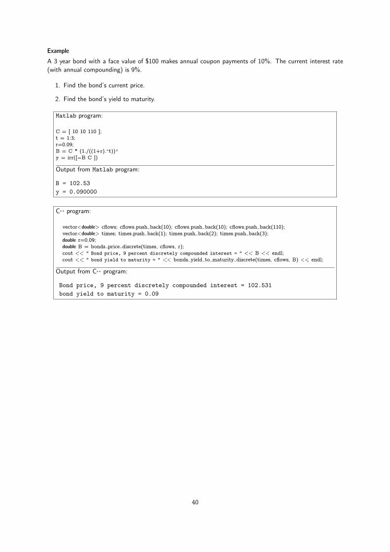
Example
A 3 year bond with a face value of $100 makes annual coupon payments of 10%. The current interest rate(with annual compounding) is 9%.
1. Find the bond’s current price.
2. Find the bond’s yield to maturity.
Matlab program:
C = [ 10 10 110 ];t = 1:3;r=0.09;B = C * (1./((1+r).^t))’y = irr([�B C ])
Output from Matlab program:
B = 102.53y = 0.090000
C++ program:
vector<double> cflows; cflows.push back(10); cflows.push back(10); cflows.push back(110);vector<double> times; times.push back(1); times.push back(2); times.push back(3);double r=0.09;double B = bonds price discrete(times, cflows, r);cout << " Bond price, 9 percent discretely compounded interest = " << B << endl;cout << " bond yield to maturity = " << bonds yield to maturity discrete(times, cflows, B) << endl;
Output from C++ program:
Bond price, 9 percent discretely compounded interest = 102.531bond yield to maturity = 0.09
40
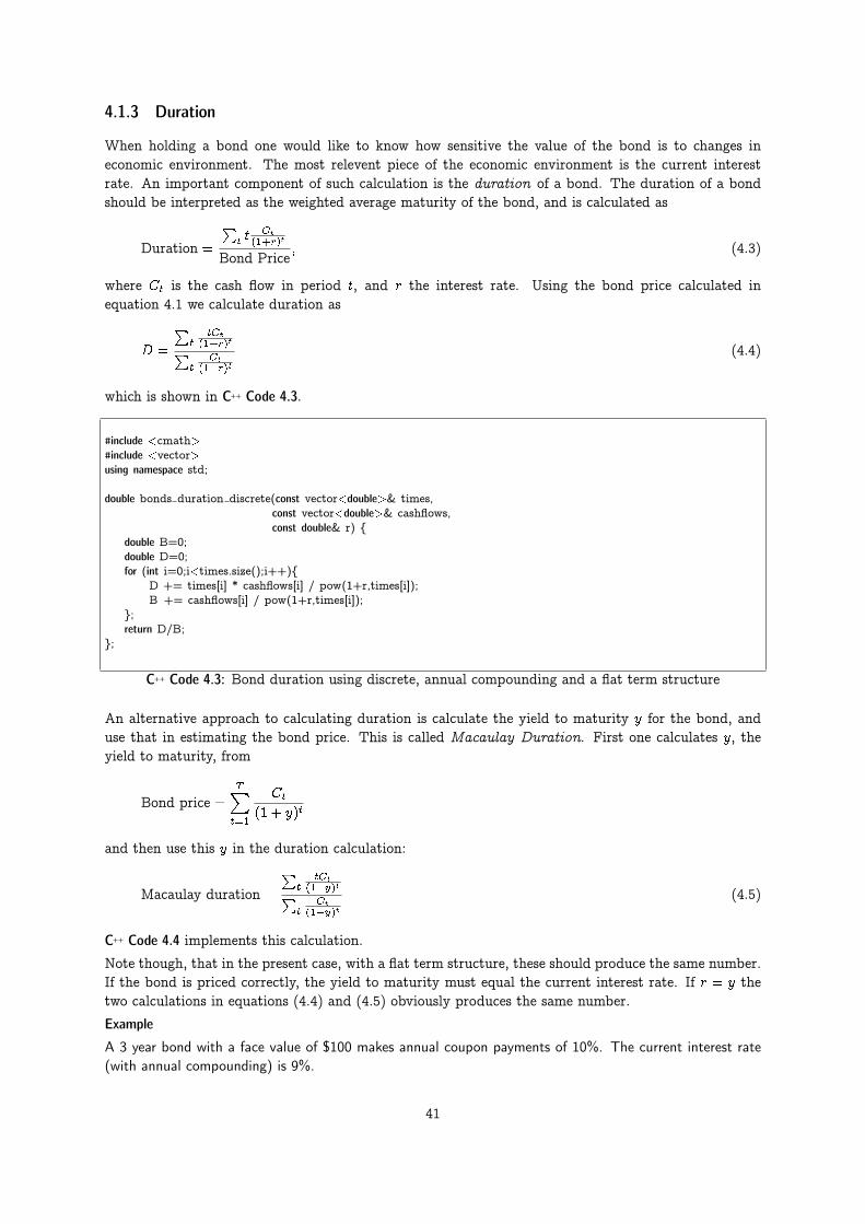
4.1.3 Duration
When holding a bond one would like to know how sensitive the value of the bond is to changes ineconomic environment. The most relevent piece of the economic environment is the current interestrate. An important component of such calculation is the duration of a bond. The duration of a bondshould be interpreted as the weighted average maturity of the bond, and is calculated as
Duration =
Pt t
Ct
(1+r)t
Bond Price; (4.3)
where Ct is the cash flow in period t, and r the interest rate. Using the bond price calculated inequation 4.1 we calculate duration as
D =
Pt
tCt
(1+r)tPt
Ct
(1+r)t
(4.4)
which is shown in C++ Code 4.3.
#include <cmath>#include <vector>using namespace std;
double bonds duration discrete(const vector<double>& times,const vector<double>& cashflows,const double& r) {
double B=0;double D=0;for (int i=0;i<times.size();i++){
D += times[i] * cashflows[i] / pow(1+r,times[i]);B += cashflows[i] / pow(1+r,times[i]);
};return D/B;
};
C++ Code 4.3: Bond duration using discrete, annual compounding and a flat term structure
An alternative approach to calculating duration is calculate the yield to maturity y for the bond, anduse that in estimating the bond price. This is called Macaulay Duration. First one calculates y, theyield to maturity, from
Bond price =TXt=1
Ct
(1 + y)t
and then use this y in the duration calculation:
Macaulay duration =
Pt
tCt
(1+y)tPt
Ct
(1+y)t
(4.5)
C++ Code 4.4 implements this calculation.
Note though, that in the present case, with a flat term structure, these should produce the same number.If the bond is priced correctly, the yield to maturity must equal the current interest rate. If r = y thetwo calculations in equations (4.4) and (4.5) obviously produces the same number.
Example
A 3 year bond with a face value of $100 makes annual coupon payments of 10%. The current interest rate(with annual compounding) is 9%.
41
#include "fin_recipes.h"
double bonds duration macaulay discrete(const vector<double>& times,const vector<double>& cashflows,const double& bond price) {
double y = bonds yield to maturity discrete(times, cashflows, bond price);return bonds duration discrete(times, cashflows, y); // use YTM in duration calculation
};
C++ Code 4.4: Calculating the Macaulay duration of a bond
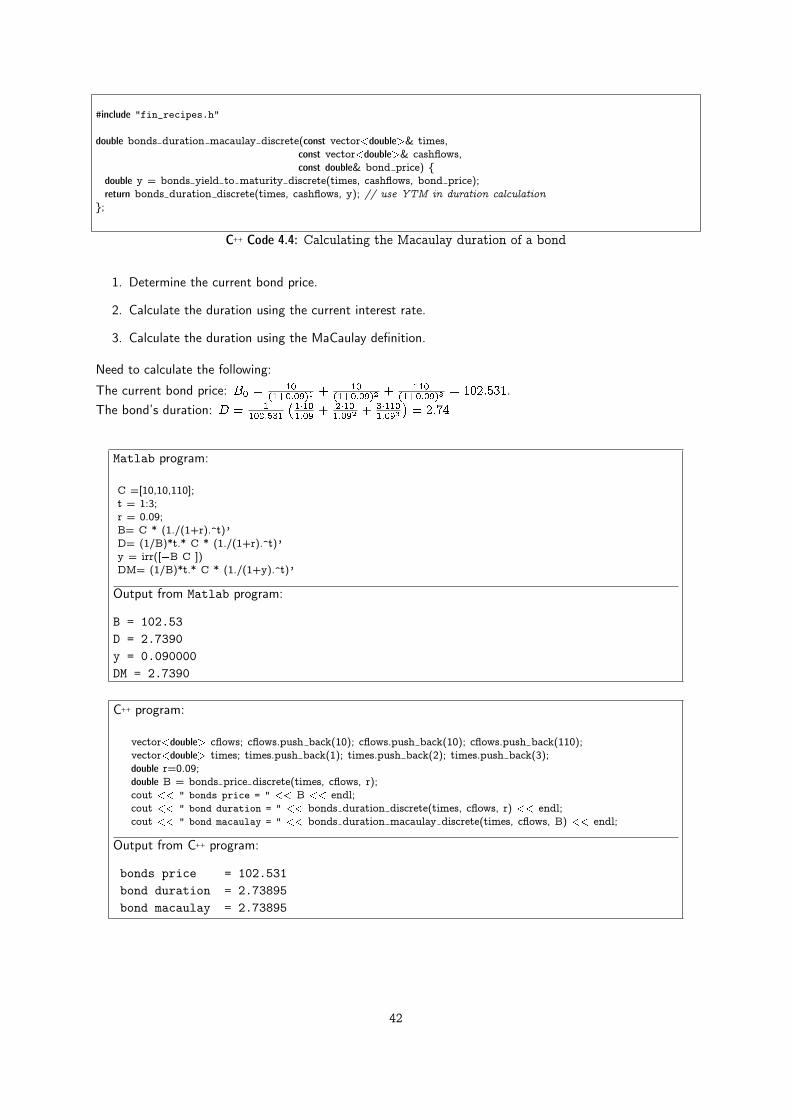
1. Determine the current bond price.
2. Calculate the duration using the current interest rate.
3. Calculate the duration using the MaCaulay definition.
Need to calculate the following:
The current bond price: B0 =10
(1+0:09)1 + 10(1+0:09)2 + 110
(1+0:09)3 = 102:531.The bond’s duration: D = 1
102:531
�1�101:09 +
2�101:092 + 3�110
1:093
�= 2:74
Matlab program:
C =[10,10,110];t = 1:3;r = 0.09;B= C * (1./(1+r).^t)’D= (1/B)*t.* C * (1./(1+r).^t)’y = irr([�B C ])DM= (1/B)*t.* C * (1./(1+y).^t)’
Output from Matlab program:
B = 102.53D = 2.7390y = 0.090000DM = 2.7390
C++ program:
vector<double> cflows; cflows.push back(10); cflows.push back(10); cflows.push back(110);vector<double> times; times.push back(1); times.push back(2); times.push back(3);double r=0.09;double B = bonds price discrete(times, cflows, r);cout << " bonds price = " << B << endl;cout << " bond duration = " << bonds duration discrete(times, cflows, r) << endl;cout << " bond macaulay = " << bonds duration macaulay discrete(times, cflows, B) << endl;
Output from C++ program:
bonds price = 102.531bond duration = 2.73895bond macaulay = 2.73895
42
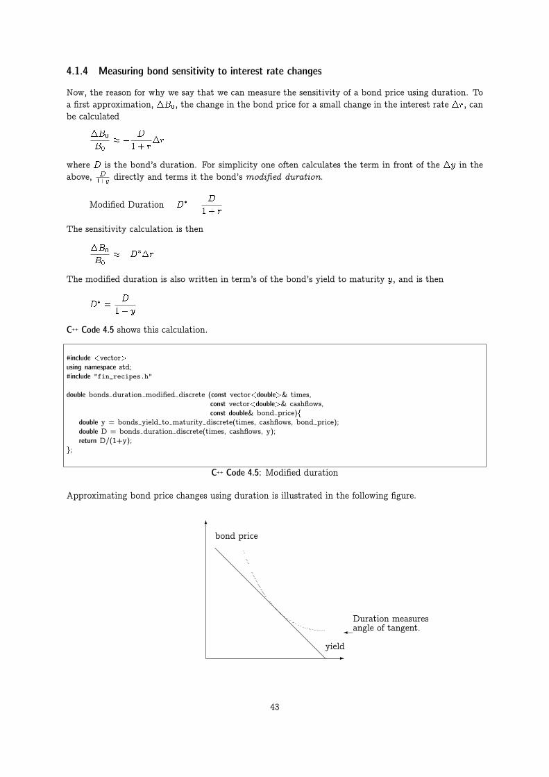
4.1.4 Measuring bond sensitivity to interest rate changes
Now, the reason for why we say that we can measure the sensitivity of a bond price using duration. Toa first approximation, �B0, the change in the bond price for a small change in the interest rate �r, canbe calculated
�B0
B0� � D
1 + r�r
where D is the bond’s duration. For simplicity one often calculates the term in front of the �y in theabove, D
1+y directly and terms it the bond’s modified duration.
Modified Duration = D� =D
1 + r
The sensitivity calculation is then
�B0
B0� �D��r
The modified duration is also written in term’s of the bond’s yield to maturity y, and is then
D� =D
1 + y
C++ Code 4.5 shows this calculation.
#include <vector>using namespace std;#include "fin_recipes.h"
double bonds duration modified discrete (const vector<double>& times,const vector<double>& cashflows,const double& bond price){
double y = bonds yield to maturity discrete(times, cashflows, bond price);double D = bonds duration discrete(times, cashflows, y);return D/(1+y);
};
C++ Code 4.5: Modified duration
Approximating bond price changes using duration is illustrated in the following figure.
-
6
@@@@@@@@@@@@
bond price
yield
Duration measuresangle of tangent.�
43

The modified duration measures the angle of the tangent at the current bond yield. Approximatingthe change in bond price with duration is thus only a first order approximation. To improve on thisapproximation we also need to account for the curvature in the relationship between bond price andinterest rate. To quantify this curvature we calculate the convexity of a bond.
Convexity = Cx =1
B0
1
(1 + r)2
TXt=1
(t+ t2)Ct
(1 + r)t(4.6)
This calculation is implemented in C++ Code 4.6. To improve on the estimate of how the bond price
#include <cmath>#include "fin_recipes.h"
double bonds convexity discrete(const vector<double>& times,const vector<double>& cashflows,const double& r) {
double Cx=0;for (int i=0;i<times.size();i++){
Cx+= cashflows[i]*times[i]*(times[i]+1)/(pow((1+r),times[i]));};double B=bonds price discrete(times, cashflows, r);return (Cx/(pow(1+r,2)))/B;
};
C++ Code 4.6: Bond convexity with a flat term structure and annual compounding
change when the interest rates changes you will then calculate
�B0
B0� �D��y +
1
2Cx (�y)
2
Formula 4.1 summarizes the above calculations.
Bond Price (B0)
B0 =
TXt=1
Ct
(1 + r)t
Yield to maturity y solves
B0 =
TXt=1
Ct
(1 + y)t
Duration (D)
D =1
B0
TXt=1
tCt
(1 + r)t
Macaulay duration
D =1
B0
TXt=1
tCt
(1 + y)t
Modified duration
D� =D
1 + y
Convexity (Cx)
Cx =1
B0
1
(1 + r)2
TXt=1
(t+ t2)Ct
(1 + r)t
Approximating bond price changes
�B0
B0� �D��y
�B0
B0� �D��y +
1
2� Cx� (�y)2
Ct: Cash flow at time t, r: interest rate, y: bond yield to maturity, B0: current bond price. Bond pays coupon at evenly spaceddates t = 1; 2; 3 : : : ; T .
Formula 4.1: Bond pricing formulas with a flat term structure and discrete, annual compounding
44

Example
A 3 year bond with a face value of $100 makes annual coupon payments of 10%. The current interest rate(with annual compounding) is 9%.
1. Determine the current bond price.
2. Suppose the interest rate changes to 10%, determine the new price of the bond by direct calculation.
3. Use duration to estimate the new price and compare it to the correct price.
4. Use convexity to improve on the estimate using duration only.
Need to calculate the following:
The current bond price: B0 =10
(1+0:09)1 + 10(1+0:09)2 + 110
(1+0:09)3 = 102:531.The bond’s duration: D = 1
102:531
�1�101:09 +
2�101:092 + 3�110
1:093
�= 2:74
The modified duration: D� = D1+r = 2:74
1:09 = 2:51.
The convexity: Cx = 1(1+0:09)2
1102:531
�(1+1)�10
1:09 + (22+2)�101:092 + (3+32)�110
1:093
�= 8:93.
Here are the calculations:
Matlab program:
C =[10,10,110];t = 1:3;r = 0.09;B= C * (1./(1+r).^t)’D= (1/B)*t.* C * (1./(1+r).^t)’Cx= (1/(1+r)^2) * (1/B)*t.^2.*C * (1./(1+r).^t)’newB=C* (1./(1+0.1).^t)’
Output from Matlab program:
B = 102.53D = 2.7390Cx = 6.6272newB = 100.000
C++ program:
vector<double> cflows; cflows.push back(10); cflows.push back(10); cflows.push back(110);vector<double> times; times.push back(1); times.push back(2); times.push back(3);double r=0.09;double B = bonds price discrete(times, cflows, r);cout << " bonds price = " << B << endl;cout << " bond duration = " << bonds duration discrete(times, cflows, r) << endl;cout << " bond duration modified = " << bonds duration modified discrete(times, cflows, B) << endl;cout << " bond convexity =" << bonds convexity discrete(times, cflows, r) << endl;cout << " new bond price = " << bonds price discrete(times, cflows, 0.1);
Output from C++ program:
bonds price = 102.531bond duration = 2.73895bond duration modified = 2.5128bond convexity =8.93248new bond price = 100
45

Using these numbers to answer the questions, let us see what happens when the interest rate increases to 10%.This means the bond will be selling at par, equal to 100, which can be confirmed with direct computation:
B0 =10
(1 + 0:1)1+
10
(1 + 0:1)2+
110
(1 + 0:1)3= 100
Using duration to estimate the change in the bond price for a unit change in the interest rate:
�B0
B0= �D��y = �2:51 � 0:01 = �0:0251
Using this duration based number to estimate the new bond price.
B = B0 +
��B0
B0
�B0 = 102:531� 0:0251 � 102:531 = 99:957
Additionally using convexity in estimating the change in the bond price:
�B0
B0= �D��y +
1
2Cxy
2 = �2:51 � 0:01 + 1
28:93(0:01)2 = �0:0251 + 0:00044 = �0:02465
B = 102:531
�1 +
��B0
B0
�B0
�= 102:531(1� 0:02465) = 100:0036
Exercise 4.1.
Perpetual duration [4]
The term structure is flat with annual compounding. Consider the pricing of a perpetual bond. Let C be theper period cash flow
B0 =
1Xt=1
C
(1 + r)t=C
r
1. Determine the first derivative of the price with respect to the interest rate.
2. Find the duration of the bond.
Exercise 4.2.
[5]
Consider an equally weighted portfolio of two bonds, A and B. Bond A is a zero coupon bond with 1 year tomaturity. Bond B is a zero coupon bond with 3 years to maturity. Both bonds have face values of 100. Thecurrent interest rate is 5%.
1. Determine the bond prices.
2. Your portfolio is currently worth 2000. Find the number of each bond invested.
3. Determine the duration of the portfolio.
4. Determine the convexity of your position.
46

4.2 Continously compounded interest
We will go over the same concepts as covered in the previous section on bond pricing. There are certainsubtle differences in the calculations. Formula 4.2 corresponds to the earlier summary in formula 4.1.
Bond Price B0:
B0 =Xi
e�rti)Cti
Yield to maturity y solves:
B0 =Xi
Ctie�yti
Duration D:
D =1
B0
Xi
tiCtie�rti
Macaulay duration
D =1
B0
Xi
tiCtie�yti
Convexity Cx:
Cx =1
B0
Xi
Ctit2i e�rti
Approximating bond price changes
�B0
B0� �D�y
�B0
B0� �D�y +
1
2� Cx� (�y)2
Bond paying cash flows Ct1 ; Ct2 ; : : : at times t1; t2; : : :. Notation: B0: current bond price. e: natural exponent.
Formula 4.2: Bond pricing formulas with continously compounded interest and a flat term structure
Some important differences is worth pointing out. When using continously compounded interest, onedoes not need the concept of modified duration. In the continously compounded case one uses thecalculated duration directly to approximate bond changes, as seen in the formulas describing the ap-proximation of bond price changes. Note also the difference in the convexity calculation, one does notdivide by (1 + y)2 in the continously compounded formula, as was done in the discrete case.
C++ Code 4.7, C++ Code 4.8, C++ Code 4.9 and C++ Code 4.10 show continously compounded analogs of theearlier codes for the discretely compounded case.
#include <cmath>#include <vector>using namespace std;
double bonds price(const vector<double>& cashflow times,const vector<double>& cashflows,const double& r) {
double p=0;for (int i=0;i<cashflow times.size();i++) {
p += exp(�r*cashflow times[i])*cashflows[i];};return p;
};
C++ Code 4.7: Bond price calculation with continously compounded interest and a flat term structure
47

#include <cmath>#include <vector>using namespace std;
double bonds duration(const vector<double>& cashflow times,const vector<double>& cashflows,const double& r) {
double S=0;double D1=0;for (int i=0;i<cashflow times.size();i++){
S += cashflows[i] * exp(�r*cashflow times[i]);D1 += cashflow times[i] * cashflows[i] * exp(�r*cashflow times[i]);
};return D1 / S;
};
C++ Code 4.8: Bond duration calculation with continously compounded interest and a flat term structure
#include "fin_recipes.h"
double bonds duration macaulay(const vector<double>& cashflow times,const vector<double>& cashflows,const double& bond price) {
double y = bonds yield to maturity(cashflow times, cashflows, bond price);return bonds duration(cashflow times, cashflows, y); // use YTM in duration
};
C++ Code 4.9: Calculating the Macaulay duration of a bond with continously compounded interest and aflat term structure
#include <cmath>#include "fin_recipes.h"
double bonds convexity(const vector<double>& times,const vector<double>& cashflows,const double& r ) {
double C=0;for (int i=0;i<times.size();i++){
C += cashflows[i] * pow(times[i],2) * exp(�r*times[i]);};double B=bonds price(times, cashflows,r);return C/B;
};
C++ Code 4.10: Bond convexity calculation with continously compounded interest and a flat term structure
48
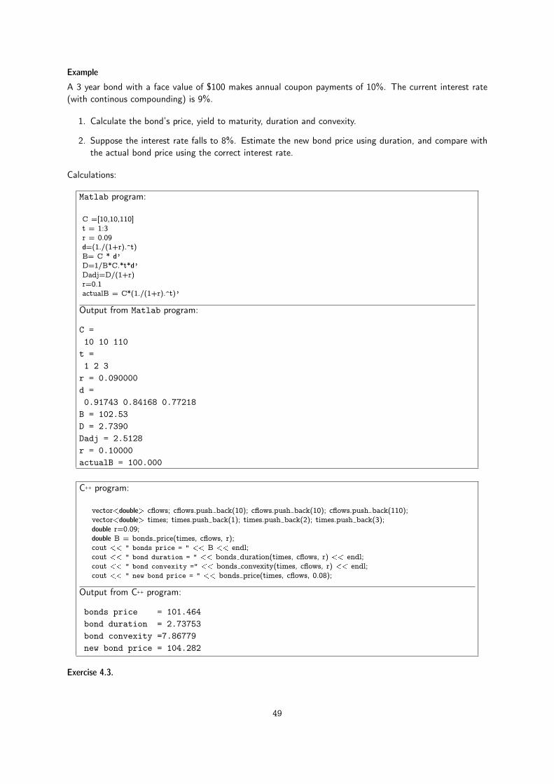
Example
A 3 year bond with a face value of $100 makes annual coupon payments of 10%. The current interest rate(with continous compounding) is 9%.
1. Calculate the bond’s price, yield to maturity, duration and convexity.
2. Suppose the interest rate falls to 8%. Estimate the new bond price using duration, and compare withthe actual bond price using the correct interest rate.
Calculations:
Matlab program:
C =[10,10,110]t = 1:3r = 0.09d=(1./(1+r).^t)B= C * d’D=1/B*C.*t*d’Dadj=D/(1+r)r=0.1actualB = C*(1./(1+r).^t)’
Output from Matlab program:
C =10 10 110t =1 2 3r = 0.090000d =0.91743 0.84168 0.77218B = 102.53D = 2.7390Dadj = 2.5128r = 0.10000actualB = 100.000
C++ program:
vector<double> cflows; cflows.push back(10); cflows.push back(10); cflows.push back(110);vector<double> times; times.push back(1); times.push back(2); times.push back(3);double r=0.09;double B = bonds price(times, cflows, r);cout << " bonds price = " << B << endl;cout << " bond duration = " << bonds duration(times, cflows, r) << endl;cout << " bond convexity =" << bonds convexity(times, cflows, r) << endl;cout << " new bond price = " << bonds price(times, cflows, 0.08);
Output from C++ program:
bonds price = 101.464bond duration = 2.73753bond convexity =7.86779new bond price = 104.282
Exercise 4.3.
49
The term structure is flat, and compounding is continous. Consider two definitions of duration, the “usual”definition D = 1
B0
Pi tiCtie
�rti and the Macaulay defintion: D = 1B0
Pi tiCtie
�yti , where B0 is the currentbond price, Cti is the coupon payment at date ti, r is the current interest rate and y is the bond’s yield tomaturity.
1. Show that these two definitions will produce the same number if the bond is correctly priced.
4.3 Further readings
The material in this chapter is covered in most standard textbooks on investments (e.g. Bodie et al.(2007), Haugen (2001) or Sharpe et al. (1999)). More details can be found in textbooks on fixed income,such as Sundaresan (2001).
50

Chapter 5
The term structure of interest rates and anobject lesson
Contents5.1 The interchangeability of discount factors, spot interest rates and forward interest rates . . . . . 525.2 The term structure as an object . . . . . . . . . . . . . . . . . . . . . . . . . . . . . . . . . . 55
5.2.1 Base class . . . . . . . . . . . . . . . . . . . . . . . . . . . . . . . . . . . . . . . 555.2.2 Flat term structure. . . . . . . . . . . . . . . . . . . . . . . . . . . . . . . . . . 57
5.3 Using the currently observed term structure. . . . . . . . . . . . . . . . . . . . . . . . . . . . 585.3.1 Linear Interpolation. . . . . . . . . . . . . . . . . . . . . . . . . . . . . . . . . . 595.3.2 Interpolated term structure class. . . . . . . . . . . . . . . . . . . . . . . . . . . 61
5.4 Bond calculations with a general term structure and continous compounding . . . . . . . . . . . 64
In this chapter we expand on the analysis of the previous chapter by relaxing the “one interest rate”assumption used there and allow the spot rates to change as you change the time you are discountingover.
Recall that we said that the present value of a set of cash flows is calculated as
PV =
NXi=1
dtiCti
-0 t1 t2 tN
Ct1 Ct2 CtN
time
�dt1Ct1
�dt2Ct2
�dtNCtN
To make this applicable to cash flows received at any future date t we potentially need an infinitenumber of discount factors dt. This is not feasible, so some lower dimensional way needs to be found toapproximate dt, but with more flexibility than the extremely strong assumption that there is one fixedinterest rate r, and that the discount factor for any time t is calculated as either dt = 1=(1+r)t (discretecompounding), or dt = e�rt (continuous compounding), which we used in the previous chapter.
51

In this chapter we first show that this approximation of the discount factors can be done in either termsof discount factors directly, interest rates, or forward rates. Either of these are useful ways of formulatinga term structure, and either of them can be used, since there are one to one transformations betweeneither of these three. We then go on to demonstrate how a feature of C++, the ability to create an abstractdatatype as an object, or class, is very useful for the particular application of defining and using a termstructure. It is in fact this particular application, to create a term structure class, which really illustratesthe power of C++, and why you want to use an object oriented language instead of classical langues likeFORTRAN and C, or matrix languages like Gauss or Matlab for many financial calculations.
5.1 The interchangeability of discount factors, spot interest rates and forwardinterest rates
The term structure can be specified in terms of either discount factors, spot interest rates or forwardinterest rates. A discount factor is the current price for a future (time t) payment of one dollar. Tofind the current value PV of a cash flow Ct, we calculate PV = dtCt. This discount factor can also bespecified in terms of interest rates, where we let rt be the relevant interest rate (spot rate) for discountinga t-period cashflow. Then we know that the present value PV = e�rttCt. Since these two methods ofcalculating the present value must be consistent,
PV = dtCt = e�rttCt
and hence
dt = e�rtt
Note that this equation calculates dt given rt. Rearranging this equation we find the spot rate rt interms of discount factors
rt =� ln(dt)
t
An alternative concept that is very useful is a forward interest rate, the yield on borrowing at somefuture date t1 and repaying it at a later date t2. Let ft1;t2 be this interest rate. If we invest one dollartoday, at the current spot rate spot rate till period t1 and the forward rate for the period from t1 to t2(which is what you would have to do to make an actual investment), you would get the following futurevalue
FV = ert1 t1eft1;t2 (t2�t1)
The present value of this forward value using the time t2 discount factor has to equal one:
dt2FV = 1
These considerations are enough to calculate the relevant transforms. The forward rate for borrowing attime t1 for delivery at time t2 is calculated as
ft1;t2 =� ln
�dt2dt1
�t2 � t1
=ln�dt1dt2
�t2 � t1
The forward rate can also be calculated directly from yields as
ft1;t2 = rt2t2
t2 � t1� rt1
t1t2 � t1
52

dt = e�rtt
rt =� ln(dt)
t
ft1;t2 =ln�dt1dt2
�t2 � t1
ft1;t2 = rt2t2
t2 � t1� rt1
t1t2 � t1
Notation: dt discount factor for payment at time t, rt: spot rate applying to cash flows at time t. ft1;t2 forward rate betweentime t1 and t2, i.e. the interest rate you would agree on today on the future transactions.
#include <cmath>using namespace std;
double term structure yield from discount factor(const double& d t, const double& t) {return (�log(d t)/t);
}
double term structure discount factor from yield(const double& r, const double& t) {return exp(�r*t);
};
double term structure forward rate from discount factors(const double& d t1, const double& d t2,const double& time) {
return (log (d t1/d t2))/time;};
double term structure forward rate from yields(const double& r t1, const double& r t2,const double& t1, const double& t2) {
return r t2*t2/(t2�t1)�r t1*t1/(t2�t1);};
C++ Code 5.1: Term structure transformations
C++ Code 5.1 shows the implementation of these transformations.
Example
You are given the one period spot rate r1 = 5% and the two period discount factor d2 = 0:9. Calculate thetwo period spot rate and the forward rate from 1 to 2.
53
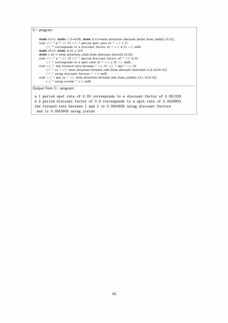
C++ program:
double t1=1; double r t1=0.05; double d t1=term structure discount factor from yield(r t1,t1);cout << " a " << t1 << " period spot rate of " << r t1
<< " corresponds to a discount factor of " << d t1 << endl;double t2=2; double d t2 = 0.9;double r t2 = term structure yield from discount factor(d t2,t2);cout << " a " << t2 << " period discount factor of " << d t2
<< " corresponds to a spot rate of " << r t2 << endl;cout << " the forward rate between " << t1 << " and " << t2
<< " is " << term structure forward rate from discount factors(d t1,d t2,t2�t1)<< " using discount factors " << endl;
cout << " and is " << term structure forward rate from yields(r t1,r t2,t1,t2)<< " using yields " << endl;
Output from C++ program:
a 1 period spot rate of 0.05 corresponds to a discount factor of 0.951229a 2 period discount factor of 0.9 corresponds to a spot rate of 0.0526803the forward rate between 1 and 2 is 0.0553605 using discount factorsand is 0.0553605 using yields
54

5.2 The term structure as an object
From the previous we see that the term structure can be described in terms of discount factors, spotrates or forward rates, but that does not help us in getting round the dimensionality problem. If wethink in terms of discount factors, for a complete specification of the current term structure one needsan infinite number of discount factors fdtgt2R+ . It is perhaps easier to think about this set of discountfactors as a function d(t), that, given a nonnegative time t, returns the discount factor. Since we haveestablished that there are three equivalent ways of defining a term structure, discount factors, spot ratesand forward rates, we can therefore describe a term structure as a collection of three different functionsthat offer different views of the same underlying object.
A term structure is an abstract object that to the user should provide
� discount factors d (prices of zero coupon bonds).
� spot rates r (yields of zero coupon bonds).
� forward rates f
for any future maturity t. The user of a term structure will not need to know how the term structure isimplemented, all that is needed is an interface that specifies the above three functions.
This is tailor made for being implemented as a C++ class. A class in C++ terms is a collection of datastructures and functions that operate on these data structures. In the present context it is a way ofspecifying the three functions.
r(t)
d(t)
f(t)
5.2.1 Base class
Header File 5.1 shows how we describe the generic term structure as a C++ class.
#ifndef TERM STRUCTURE CLASS H#define TERM STRUCTURE CLASS H
class term structure class {public:
virtual double r(const double& t) const; // yield on zero coupon bondvirtual double d(const double& t) const; // discount factor/price of zero coupon bondvirtual double f(const double& t1, const double& t2) const; // forward ratevirtual ˜term structure class();
};
#endif
Header file 5.1: Header file describing the term_structure base class
The code for these functions uses algorithms that are described earlier in this chapter for transformingbetween various views of the term structure. The term structure class merely provide a convenientinterface to these algorithms. The code is shown in C++ Code 5.2
Note that the definitions of calculations are circular. Any given specific type of term structure has toover-ride at least one of the functions r (yield), d (discount factor) or f (forward rate).
We next consider two examples of specific term structures.
55

#include "fin_recipes.h"
term structure class::˜term structure class(){};
double term structure class::f(const double& t1, const double& t2) const{double d1 = d(t1);double d2 = d(t2);return term structure forward rate from discount factors(d1,d2,t2�t1);
};
double term structure class::r(const double& t) const{return term structure yield from discount factor(d(t),t);
};
double term structure class::d(const double& t) const {return term structure discount factor from yield(r(t),t);
};
C++ Code 5.2: Default code for transformations between discount factors, spot rates and forward rates ina term structure class
56

5.2.2 Flat term structure.
The flat term structure overrides the yield member function of the base class.
The only piece of data this type of term structure needs is an interest rate.
#ifndef TERM STRUCTURE CLASS FLAT#define TERM STRUCTURE CLASS FLAT
#include "term_structure_class.h"
class term structure class flat : public term structure class {private:
double R ; // interest ratepublic:
term structure class flat(const double& r);virtual ˜term structure class flat();virtual double r(const double& t) const;void set int rate(const double& r);
};
#endif
Header file 5.2: Header file for term structure class using a flat term structure
#include "fin_recipes.h"
term structure class flat::term structure class flat(const double& r){ R = r; };
term structure class flat::˜term structure class flat(){};
double term structure class flat::r(const double& T) const { if (T>=0) return R ; return 0; };
void term structure class flat::set int rate(const double& r) { R = r; };
C++ Code 5.3: Implementing term structure class using a flat term structure
Example
The term structure is flat with r = 5%. Determine the discount factors for years 1 and 2 and the forwardrate between 1 and 2.
C++ program:
term structure class flat ts(0.05);double t1=1;cout << "discount factor t1 = " << t1 << ":" << ts.d(t1) << endl;double t2=2;cout << "discount factor t2 = " << t2 << ":" << ts.d(t2) << endl;cout << "spot rate t = " << t1 << ":" << ts.r(t1) << endl;cout << "spot rate t = " << t2 << ":" << ts.r(t2) << endl;cout << "forward rate from t1= " << t1 << " to t2= " << t2 << ":"
<< ts.f(t1,t2) << endl;
Output from C++ program:
discount factor t1 = 1:0.951229discount factor t2 = 2:0.904837spot rate t = 1:0.05spot rate t = 2:0.05forward rate from t1= 1 to t2= 2:0.05
57

5.3 Using the currently observed term structure.
A first step to a general term structure is to use market data on bond prices and interest rates to inferdiscount factors. The simplest way of presenting this problem is in terms of linear algebra. Suppose wehave three bonds with cash flows at times 1, 2 and 3.
B1 = d1C11 + d2C12 + d2C13
B2 = d1C21 + d2C22 + d2C23
B1 = d1C31 + d2C32 + d2C33
Writing this in terms of matrices24 B1
B2
B3
35 =
24 d1d2d3
3524 C11 C12 C13
C21 C22 C23
C31 C32 C33
35Solving for the discount factors24 d1
d2d3
35 =
24 C11 C12 C13
C21 C22 C23
C31 C32 C33
35�1 24 B1
B2
B3
35or
d = C�1B
using the obvious matrix definitions
B =
24 B1
B2
B3
35 d =
24 d1d2d3
35 C =
24 C11 C12 C13
C21 C22 C23
C31 C32 C33
35Example
The following set of bond and bond prices is observed:
Time (in years)Bond 0 0.5 1 1.5 2 3 4
Bond Price1 98 1002 96 1002 92 1003 118 10 10 10 1104 109 8 8 8 8 1085 112 9 9 9 9 9 109
The bonds are treasury secrurities, which can be viewed as nominally riskless.
1. For what maturities is it possible to infer discount factors?
2. Determine the implicit discount factors in the market.
3. What is the interest rates implied in this set of discount rates?
Here we can find the discount factors for maturities of 0.5,1,1.5,2,3 and 4.
58

Matlab program:
C=[100 0 0 0 0 0;0 100 0 0 0 0;0 0 100 0 0 0;10 10 10 110 0 0;8 8 8 8 108 0;9 9 9 9 9 109]B=[96 94 92 118 109 112]d=B*inv(C)’t=[0.5 1 1.5 2 3 4]r=d.^(�1./t)�1
Output from Matlab program:
C =100 0 0 0 0 00 100 0 0 0 00 0 100 0 0 010 10 10 110 0 08 8 8 8 108 09 9 9 9 9 109B =96 94 92 118 109 112d =0.96000 0.94000 0.92000 0.81636 0.73990 0.66618t =0.50000 1.00000 1.50000 2.00000 3.00000 4.00000r =0.085069 0.063830 0.057162 0.106772 0.105628 0.106884
To just use todays term structure, we need to take the observations of discount factors dt observed inthe market and use these to generate a term structure. The simplest possible way of doing this is tolinearly interpolate the currently observable discount factors.
5.3.1 Linear Interpolation.
If we are given a set of discount factors (dt) for various maturities, the simplest way to construct aterm structure is by straightforward linear interpolation between the observations we have to find anintermediate time. For many purposes this is “good enough.” This interpolation can be on either zerocoupon yields, discount factors or forward rates, we illustrate the case of linear interpolation of spot(zero coupon) rates.
Computer algorithm, linear interpolation of yields. Note that the algorithm assumes the yields are orderedin increasing order of time to maturity.
Example
You observe the following term structure of spot rates
Time r
0.1 0.10.5 0.21 0.35 0.410 0.5
Interpolate spot rates (zero rates) at times 0.1, 0.5, 1, 3, 5 and 10.
59

#include <vector>using namespace std;#include "fin_recipes.h"
double term structure yield linearly interpolated(const double& time,const vector<double>& obs times,const vector<double>& obs yields) {
// assume the yields are in increasing time to maturity order.int no obs = int(obs times.size());if (no obs<1) return 0;double t min = obs times[0];if (time <= t min) return obs yields[0]; // earlier than lowest obs.
double t max = obs times[no obs�1];if (time >= t max) return obs yields[no obs�1]; // later than latest obs
int t=1; // find which two observations we are betweenwhile ( (t<no obs) && (time>obs times[t])) { ++t; };double lambda = (obs times[t]�time)/(obs times[t]�obs times[t�1]);// by ordering assumption, time is between t-1,tdouble r = obs yields[t�1] * lambda + obs yields[t] * (1.0�lambda);return r;
};
C++ Code 5.4: Interpolated term structure from spot rates
C++ program:
vector<double> times;vector<double> yields;times.push back(0.1); times.push back(0.5); times.push back(1);yields.push back(0.1); yields.push back(0.2); yields.push back(0.3);times.push back(5); times.push back(10);yields.push back(0.4); yields.push back(0.5);cout << " yields at times: " << endl;cout << " t=0.1 " << term structure yield linearly interpolated(0.1,times,yields) << endl;cout << " t=0.5 " << term structure yield linearly interpolated(0.5,times,yields) << endl;cout << " t=1 " << term structure yield linearly interpolated(1, times,yields) << endl;cout << " t=3 " << term structure yield linearly interpolated(3, times,yields) << endl;cout << " t=5 " << term structure yield linearly interpolated(5, times,yields) << endl;cout << " t=10 " << term structure yield linearly interpolated(10, times,yields) << endl;
Output from C++ program:
yields at times:t=0.1 0.1t=0.5 0.2t=1 0.3t=3 0.35t=5 0.4t=10 0.5
60

5.3.2 Interpolated term structure class.
The interpolated term structure implemented here uses a set of observations of yields as a basis, andfor observations in between observations will interpolate between the two closest. The following onlyprovides implementations of calculation of the yield, for the other two rely on the base class code.
As shown in Header File 5.3 and C++ Code 5.5, there is some more book-keeping involved here, need tohave code that stores observations of times and yields.
#ifndef TERM STRUCTURE CLASS INTERPOLATED#define TERM STRUCTURE CLASS INTERPOLATED
#include "term_structure_class.h"#include <vector>using namespace std;
class term structure class interpolated : public term structure class {private:
vector<double> times ; // use to keep a list of yieldsvector<double> yields ;void clear();
public:term structure class interpolated();term structure class interpolated(const vector<double>& times, const vector<double>& yields);virtual ˜term structure class interpolated();term structure class interpolated(const term structure class interpolated&);term structure class interpolated operator= (const term structure class interpolated&);
int no observations() const { return times .size(); };virtual double r(const double& T) const;void set interpolated observations(vector<double>& times, vector<double>& yields);
};
#endif
Header file 5.3: Header file describing a term structure class using linear interpolation between spot rates
61

#include "fin_recipes.h"
void term structure class interpolated::clear(){times .erase(times .begin(), times .end());yields .erase(yields .begin(), yields .end());
};
term structure class interpolated::term structure class interpolated():term structure class(){clear();};
term structure class interpolated::term structure class interpolated(const vector<double>& in times,const vector<double>& in yields) {
clear();if (in times.size()!=in yields.size()) return;times = vector<double>(in times.size());yields = vector<double>(in yields.size());for (int i=0;i<in times.size();i++) {
times [i]=in times[i];yields [i]=in yields[i];
};};
term structure class interpolated::˜term structure class interpolated(){ clear();};
term structure class interpolated::term structure class interpolated(const term structure class interpolated& term) {times = vector<double> (term.no observations());yields = vector<double> (term.no observations());for (int i=0;i<term.no observations();i++){
times [i] = term.times [i];yields [i] = term.yields [i];
};};
term structure class interpolatedterm structure class interpolated::operator= (const term structure class interpolated& term) {
times = vector<double> (term.no observations());yields = vector<double> (term.no observations());for (int i=0;i<term.no observations();i++){
times [i] = term.times [i];yields [i] = term.yields [i];
};return (*this);
};
double term structure class interpolated::r(const double& T) const {return term structure yield linearly interpolated(T, times , yields );
};
voidterm structure class interpolated::set interpolated observations(vector<double>& in times,
vector<double>& in yields) {clear();if (in times.size()!=in yields.size()) return;times = vector<double>(in times.size());yields = vector<double>(in yields.size());for (int i=0;i<in times.size();i++) {
times [i]=in times[i];yields [i]=in yields[i];
};};
C++ Code 5.5: Term structure class using linear interpolation between spot rates
62

Example
Time r
0.1 0.051 0.075 0.08
Determine discount factors and spot rates at times 1 and 2, and forward rate between 1 and 2.
C++ program:
vector<double> times; times.push back(0.1);vector<double> spotrates; spotrates.push back(0.05);times.push back(1); times.push back(5);spotrates.push back(0.07);spotrates.push back(0.08);term structure class interpolated ts(times,spotrates);double t1=1;cout << "discount factor t1 = " << t1 << ":" << ts.d(t1) << endl;double t2=2;cout << "discount factor t2 = " << t2 << ":" << ts.d(t2) << endl;cout << "spot rate t = " << t1 << ":" << ts.r(t1) << endl;cout << "spot rate t = " << t2 << ":" << ts.r(t2) << endl;cout << "forward rate from t1= " << t1 << " to t2= " << t2 << ":"
<< ts.f(t1,t2) << endl;
Output from C++ program:
discount factor t1 = 1:0.932394discount factor t2 = 2:0.865022spot rate t = 1:0.07spot rate t = 2:0.0725forward rate from t1= 1 to t2= 2:0.075
63
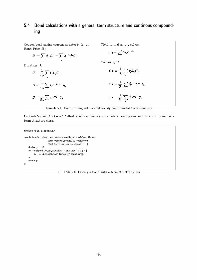
5.4 Bond calculations with a general term structure and continous compound-ing
Coupon bond paying coupons at dates t1; t2; : : ::Bond Price B0:
B0 =Xi
dtiCti =Xi
e�rti tiCti
Duration D:
D =1
B0
Xi
tidtiCti
D =1
B0
Xi
tie�rti tiCti
D =1
B0
Xi
tie�ytiCti
Yield to maturity y solves:
B0 =Xi
Ctie�yti
Convexity Cx:
Cx =1
B0
Xi
t2i dtiCti
Cx =1
B0
Xi
t2i e�rti tiCti
Cx =1
B0
Xi
t2i e�ytiCti
Formula 5.1: Bond pricing with a continously compounded term structure
C++ Code 5.6 and C++ Code 5.7 illustrates how one would calculate bond prices and duration if one has aterm structure class.
#include "fin_recipes.h"
double bonds price(const vector<double>& cashflow times,const vector<double>& cashflows,const term structure class& d) {
double p = 0;for (unsigned i=0;i<cashflow times.size();i++) {
p += d.d(cashflow times[i])*cashflows[i];};return p;
};
C++ Code 5.6: Pricing a bond with a term structure class
64

#include "fin_recipes.h"
double bonds duration(const vector<double>& cashflow times,const vector<double>& cashflow amounts,const term structure class& d ) {
double S=0;double D1=0;for (unsigned i=0;i<cashflow times.size();i++){
S += cashflow amounts[i] * d.d(cashflow times[i]);D1 += cashflow times[i] * cashflow amounts[i] * d.d(cashflow times[i]);
};return D1/S;
};
C++ Code 5.7: Calculating a bonds duration with a term structure class
#include "fin_recipes.h"#include <cmath>
double bonds convexity(const vector<double>& cashflow times,const vector<double>& cashflow amounts,const term structure class& d ) {
double B=0;double Cx=0;for (unsigned i=0;i<cashflow times.size();i++){
B += cashflow amounts[i] * d.d(cashflow times[i]);Cx += pow(cashflow times[i],2) * cashflow amounts[i] * d.d(cashflow times[i]);
};return Cx/B;
};
C++ Code 5.8: Calculating a bonds convexity with a term structure class
65
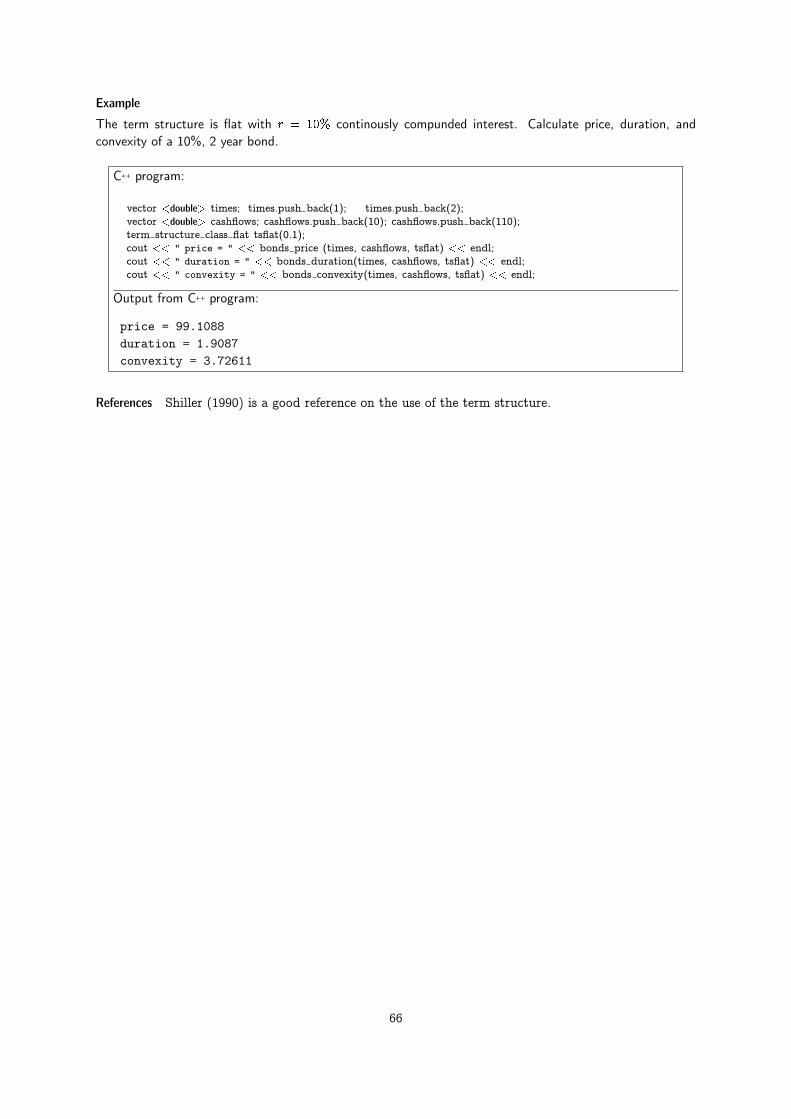
Example
The term structure is flat with r = 10% continously compunded interest. Calculate price, duration, andconvexity of a 10%, 2 year bond.
C++ program:
vector <double> times; times.push back(1); times.push back(2);vector <double> cashflows; cashflows.push back(10); cashflows.push back(110);term structure class flat tsflat(0.1);cout << " price = " << bonds price (times, cashflows, tsflat) << endl;cout << " duration = " << bonds duration(times, cashflows, tsflat) << endl;cout << " convexity = " << bonds convexity(times, cashflows, tsflat) << endl;
Output from C++ program:
price = 99.1088duration = 1.9087convexity = 3.72611
References Shiller (1990) is a good reference on the use of the term structure.
66

Chapter 6
The Mean Variance Frontier
Contents6.1 Setup . . . . . . . . . . . . . . . . . . . . . . . . . . . . . . . . . . . . . . . . . . . . . . . 676.2 The minimum variance frontier . . . . . . . . . . . . . . . . . . . . . . . . . . . . . . . . . . 696.3 Calculation of frontier portfolios . . . . . . . . . . . . . . . . . . . . . . . . . . . . . . . . . . 696.4 The global minimum variance portfolio . . . . . . . . . . . . . . . . . . . . . . . . . . . . . . 726.5 Efficient portfolios . . . . . . . . . . . . . . . . . . . . . . . . . . . . . . . . . . . . . . . . . 726.6 The zero beta portfolio . . . . . . . . . . . . . . . . . . . . . . . . . . . . . . . . . . . . . . 736.7 Allowing for a riskless asset. . . . . . . . . . . . . . . . . . . . . . . . . . . . . . . . . . . . . 736.8 Efficient sets with risk free assets. . . . . . . . . . . . . . . . . . . . . . . . . . . . . . . . . . 746.9 Short-sale constraints . . . . . . . . . . . . . . . . . . . . . . . . . . . . . . . . . . . . . . . 756.10 The Sharpe Ratio . . . . . . . . . . . . . . . . . . . . . . . . . . . . . . . . . . . . . . . . . 756.11 Equilibrium: CAPM . . . . . . . . . . . . . . . . . . . . . . . . . . . . . . . . . . . . . . . . 76
6.11.1 Treynor . . . . . . . . . . . . . . . . . . . . . . . . . . . . . . . . . . . . . . . . 766.11.2 Jensen . . . . . . . . . . . . . . . . . . . . . . . . . . . . . . . . . . . . . . . . 76
6.12 Working with Mean Variance and CAPM . . . . . . . . . . . . . . . . . . . . . . . . . . . . . 766.13 Mean variance analysis using matrix libraries . . . . . . . . . . . . . . . . . . . . . . . . . . . 77
We now discuss a classical topic in finance, mean variance analysis. This leads to ways of accounting forthe riskiness of cashflows.
Mean variance analysis concerns investors choices between portfolios of risky assets, and how an investorchooses portfolio weights. Let rp be a portfolio return. We assume that investors preferences overportfolios p satisfy a mean variance utility representation, u(p) = u(E[rp]; �(rp)), with utility increasingin expected return (@u=@E[rp] > 0) and decreasing in variance (@u=@var(rp) < 0). In this part weconsider the representation of the portfolio opportunity set of such decision makers. There are a numberof useful properties of this opportunity set which follows purely from the mathematical formulation ofthe optimization problem. It is these properties we focus on here.
6.1 Setup
We assume there exists n � 2 risky securities, with expected returns e
e =
26664E[r1]
E[r2]...
E[rn]
37775
67

and covariance matrix V:
V =
26664�(r1; r1) �(r1; r2) : : :
�(r2; r1) �(r2; r2) : : :...
�(rn; r1) : : : �(rn; rn)
37775The covariance matrix V is assumed to be invertible.
A portfolio p is defined by a set of weights w invested in the risky assets.
w =
26664!1!2...!n
37775 ;where wi is the fraction of the investors wealth invested in asset i. Note that the weights sum to one.The expected return on a portfolio is calculated as
E[rp] = w0e
and the variance of the portfolio is
�2(rp) = w0Vw
Example
An investor can invest in three assets with expected returns and variances as specified in the following table.
t Asset E[r] �2(r)
1 10% 0.202 11.5% 0.103 8% 0.15
The three assets are independent (uncorrelated).
1. Determine the expected return and standard deviation of an equally weighted portfolio of the threeassets
Matlab program:
e=[0.1 0.11 0.08]V=[ 0.2 0 0; 0 0.1 0 ; 0 0 0.15]w=1/3*[1 1 1]er= e*w’sigma=sqrt(w*V*w’)
Output from Matlab program:
e =0.100000 0.110000 0.080000V =0.20000 0.00000 0.000000.00000 0.10000 0.000000.00000 0.00000 0.15000w =0.33333 0.33333 0.33333er = 0.096667sigma = 0.22361
68

6.2 The minimum variance frontier
A portfolio is a frontier portfolio if it minimizes the variance for a given expected return, that is, afrontier portfolio p solves
wp = argminw
1
2w0Vw
subject to:
w0e = E[~rp]
w01 = 1
The set of all frontier portfolios is called the minimum variance frontier.
6.3 Calculation of frontier portfolios
Proposition 1 If the matrix V is full rank, and there are no restrictions on shortsales, the weightswp for a frontier portfolio p with mean E[~rp] can be found as
wp = g + hE[rp]
where
g =1
D(B10 � Ae0)V�1
h =1
D(Ce0 � A10)V�1
A = 10V�1e
B = e0V�1e
C = 10V�11
A =
�B A
A C
�D = BC � A2 = jAj
Proof
Any minimum variance portfolio solves the program
wp = argminw
1
2w0Vw
subject to
w0e = E[~rp]
w01 = 1
Set up the Lagrangian corresponding to this problem
L(w; �; je;V) =1
2w0Vw � �
�E[~rp]�w0e
�� (1�w01)
69
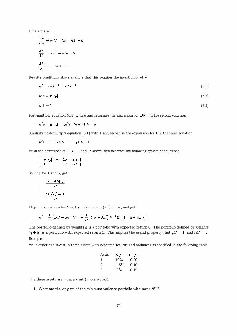
Differentiate
@L
@w= w0V � �e0 � 10 = 0
@L
@�= E[rp]�w0e = 0
@L
@ = 1�w01 = 0
Rewrite conditions above as (note that this requires the invertibility of V.
w0 = �e0V �1 � 10V�1 (6.1)
w0e = E[~rp] (6.2)
w01 = 1 (6.3)
Post-multiply equation (6.1) with e and recognise the expression for E[rp] in the second equation
w0e = E[rp] = �e0V�1e+ 10V�1e
Similarly post-multiply equation (6.1) with 1 and recognise the expression for 1 in the third equation
w01 = 1 = �e0V�11+ 10V�11
With the definitions of A, B, C and D above, this becomes the following system of equations�E[rp] = �B + A
1 = �A+ C
�Solving for � and , get
=B � AE[rp]
D
� =CE[rp]� A
D
Plug in expressions for � and into equation (6.1) above, and get
w0 =1
D
�B10 � Ae0
�V�1 +
1
D
�Ce0 � A10
�V�1
E[rp] = g + hE[rp]
The portfolio defined by weights g is a portfolio with expected return 0. The portfolio defined by weights(g+h) is a portfolio with expected return 1. This implies the useful property that g10 = 1, and h10 = 0.
Example
An investor can invest in three assets with expected returns and variances as specified in the following table.
t Asset E[r] �2(r)
1 10% 0.202 11.5% 0.103 8% 0.15
The three assets are independent (uncorrelated).
1. What are the weights of the minimum variance portfolio with mean 9%?
70

Matlab program:
e=[0.1 0.11 0.08]’V=[ 0.2 0 0; 0 0.1 0 ; 0 0 0.15]r=0.09n = length(e)a = ones(1,n)*inv(V)*eb = e’*inv(V)*ec = ones(1,n)*inv(V)*ones(n,1)A = [b a;a c]d = det(A)g = 1/d*(b*ones(1,n) � a*e’)*inv(V)h = h = 1/d*(c*e’ - a*ones(1,n))*inv(V)w=g+h*r
Output from Matlab program:
e =0.1000000.1100000.080000V =0.20000 0.00000 0.000000.00000 0.10000 0.000000.00000 0.00000 0.15000r = 0.090000n = 3a = 2.1333b = 0.21367c = 21.667A =0.21367 2.133332.13333 21.66667d = 0.078333g =0.021277 -2.680851 3.659574h =2.1277 31.9149 -34.0426w =0.21277 0.19149 0.59574
This calculation is put into a Matlab function in Matlab Code 6.1.
function w = min variance portfolio(e,V,r)n = length(e);a = ones(1,n)*inv(V)*e;b = e’*inv(V)*e;c = ones(1,n)*inv(V)*ones(n,1);A = [b a;a c];d = det(A);g = 1/d*(b*ones(1,n) � a*e’)*inv(V);h = h = 1/d*(c*e’ - a*ones(1,n))*inv(V);w=g+h*r;
end
Matlab Code 6.1: Calculation of minimum variance portfolio for given return
71

Calculating the weights of the minimum variance portfolio given an interest rate
wp = g + hE[rp]
where
g =1
D(B10 � Ae0)V�1
h =1
D(Ce0 � A10)V�1
A = 10V�1e
B = e0V�1e
C = 10V�11
D = BC � A2 =
Notation: rp desired portfolio returns.V: covariance matrix of asset returns. e: vector of expected asset returns.
6.4 The global minimum variance portfolio
The portfolio that minimizes variance regardless of expected return is called the global minimum vari-ance portfolio. Let mvp be the global minimum variance portfolio.
Proposition 2 (Global Minimum Variance Portfolio) The global minimum variance portfolio has weights
w0mvp =
�10V�11
��110V�1 =
1
C10V�1;
expected return E[rmvp] =AC and variance var(rmvp) =
1C .
E[r]
�(r)-
6
AC
p1C
6.5 Efficient portfolios
Portfolios on the minimum variance frontier with expected returns higher than or equal to E[rmvp] arecalled efficient portfolios.
E[r]
�(r)-
6
E[rmvp]
�(rmvp)
72

6.6 The zero beta portfolio
Proposition 3 For any portfolio p on the frontier, there is a frontier portfolio zc(p) satisfying
cov(rzc(p); rp) = 0:
This portfolio is called the zero beta portfolio relative to p. The zero beta portfolio zb(p) has return
E[rzc(p)] =A
C�
DC2
E[rp]� AC
-
6
mvpsszc(p)E[rzc(p)]
sp
Note that if p is an efficient portfolio on the mean variance frontier then zc(p) is inefficient. Conversely,if p is inefficient zc(p) is efficient.
E[r]
-
6
�(r)
�������sp
szc(p)smvp
6.7 Allowing for a riskless asset.
Suppose have N risky assets with weights w and one riskless assets with return rf .
Intuitively, the return on a portfolio with a mix of risky and risky assets can be written as
E[rp] = weight in risky� return risky + weight riskless � rf
which in vector form is:
E[rp] = w0e+ (1�w01)rf
Proposition 4 An efficient portfolio in the presence of a riskless asset has the weights
wp = V�1(e� 1rf )E[rp]� rf
H
where
H = (e� 1rf )0V�1(e� 1rf )
73

The variance of the efficient portfolio is
�2(rp) =(E[rp]� rf )
2
H
Note that standard deviation is a linear function of E[rp]. The efficient set is a line in mean-standarddeviation space.
6.8 Efficient sets with risk free assets.
Suppose rf < AC . Then the efficient set is the line from (0; rf ) through tangency on the efficient set of
risky assets.
E[r]
-
6
�(r)
������se
rf@@@@@@
smvp
AC
p1C
Suppose rf > AC . Then the efficient set is the two half-lines starting from (0; rf ).
E[r]
-
6
�(r)
������
se
rf@@@@@@
smvp
AC
p1C
If rf = AC , the weight in the risk free asset is one. The risky portfolio is an zero investment portfolio.
The efficient set consists of two asymptotes toward the efficient set of risky assets.
74

E[r]
-
6
�(r)
������
@@@@@@
smvp
AC
p1C
6.9 Short-sale constraints
So far the analysis has put no restrictions on the set of weights wp that defines the minimum variancefrontier. For practical applications, existence of negative weights is problematic, since this involvesselling securities short.
This has led to the investigation of restricted mean variance frontiers, where the weights are constrainedto be non-negative.
Definition 1 A short sale resctricted minimum variance portfolio p solves
wp = argminw
1
2w0Vw
subject to
w0e = E[~rp]
w01 = 1
w0 � 0
Such short sale resctricted minimum variance portfolio portfolios are much harder to deal with ana-lytically, since they do not admit a general solution, one rather has to investigate the Kuhn-Tuckerconditions for corner solutions etc. To deal with this problem in practice one will use a subroutine forsolving constrained optimization problems.
6.10 The Sharpe Ratio
The Sharpe ratio of a given portfolio p is defined as
Sp =E[rp]� rf�(rp)
The Sharpe ratio Sp of a portfolio p is the slope of the line in mean-standard deviations space from therisk free rate through p. Note that in the case with a risk free asset, the tangency portfolio has themaximal Sharpe Ratio on the efficient frontier.
75
6.11 Equilibrium: CAPM
Under certain additional assumptions, an economy of mean variance optimizers will aggregate to aneconomy where the Capital Asset Pricing Model (CAPM) holds. Under the CAPM, any asset returnswill satisfy.
E[ri] = rf + �i(E[rm]� rf )
where ri is the return on asset i, rf the return on the risk free asset,
6.11.1 Treynor
Tp =rp � rf�p
6.11.2 Jensen
�p = rp � (rf + �p(rm � rf )
6.12 Working with Mean Variance and CAPM
The computational problems in mean variance optimization and the CAPM are not major, except forthe case of short sales constrained portfolios (quadratic programming). The issues of more concern isestimation of parameters such as covariances and betas.
function s= sharpe(r,rf)s=(mean(r)�mean(rf))/std(r�rf);
endfunction
Matlab Code 6.2: Sharpe Ratio
function t = treynor(r, rm, rf)beta = cov(r,rm)/var(rm);t = (mean(r�rf))/beta;
endfunction
Matlab Code 6.3: Treynor Ratio
function alpha = jensen(r, rm, rf)beta = cov(r,rm)/var(rm);alpha = mean(r) � (rf+beta*(mean(rm)�rf));
endfunction
Matlab Code 6.4: Jensens alpha
Readings and Sources The classical sources for this material are Merton (1972) and Roll (1977a). (Huangand Litzenberger, 1988, Ch 3) has a good textbook discussion of it.
76
6.13 Mean variance analysis using matrix libraries
Let us now consider how to implement mean variance analysis in C++. As shown using Matlab, thecalculations are relatively simple matrix expressions. To implement the calculations in C++ the best wayof doing it is to use a linear algebra class to deal with the calculations. For illustrative purposes we willshow usage of two different matrix classes, Newmat and IT++. These classes are described in more detailin an appendix, with some references to how to obtain and install them.
In C++ Code 6.1 and C++ Code 6.2 we show how to do the basic mean variance calculations, calculatingmeans and standard deviations, using the two classes. Note the similarity to using Matlab in the waythe matrix and vector multiplications are carried out. Note also an important difference between thetwo classes. In IT++ the indexing of elements start at zero, the usual C++ way. Hence, when adressingelement tmp(0,0) in the IT++ example we are pulling the first element. In Newmat the default indexingstarts at one, the Matlab way. Therefore, in adressing tmp(1,1) in the Newmat example we are alsopulling the first element. This serves as a warning to read the documentation carefully, the “off by one”error is a very common occurrence when mixing libraries like this.
#include <cmath>using namespace std;
#include <itpp/itbase.h>using namespace itpp;
double mv calculate mean(const vec& e, const vec& w){vec tmp = e.transpose()*w;return tmp(0);
};
double mv calculate variance(const mat& V, const vec& w){mat tmp = w.transpose()*V*w;return tmp(0,0);
};
double mv calculate st dev(const mat& V, const vec& w){double var = mv calculate variance(V,w);return sqrt(var);
};
C++ Code 6.1: Mean variance calculations using IT++
Example
Mean variance calculations.
e =
�0:05
0:1
�
V =
�1:0 0:0
0:0 1:0
�Calculate mean, variance and stdev for portfolio
w =
�0:5
0:5
�
77

#include <cmath>using namespace std;
#include "newmat.h"using namespace NEWMAT;
double mv calculate mean(const Matrix& e, const Matrix& w){Matrix tmp = e.t()*w;return tmp(1,1);
};
double mv calculate variance(const Matrix& V, const Matrix& w){Matrix tmp = w.t()*V*w;return tmp(1,1);
};
double mv calculate st dev(const Matrix& V, const Matrix& w){double var = mv calculate variance(V,w);return sqrt(var);
};
C++ Code 6.2: Mean variance calculations using Newmat
C++ program:
cout << "Simple example of mean variance calculations " << endl;Matrix e(2,1);e(1,1)=0.05; e(2,1)=0.1;Matrix V(2,2);V(1,1)=1.0; V(2,1)=0.0;V(1,2)=0.0; V(2,2)=1.0;Matrix w(2,1);w(1,1)=0.5;w(2,1)=0.5;cout << " mean " << mv calculate mean(e,w) << endl;cout << " variance " << mv calculate variance(V,w) << endl;cout << " stdev " << mv calculate st dev(V,w) << endl;
Output from C++ program:
Simple example of mean variance calculationsmean 0.075variance 0.5stdev 0.707107
78
In C++ Code 6.4 and C++ Code 6.3 we show how to calculate the mean variance optimal portfolio for a givenrequired return. This is the case where there are no constraints on the weight, and we use the analyticalsolution directly.
#include "newmat.h"using namespace NEWMAT;
ReturnMatrix mv calculate portfolio given mean unconstrained(const Matrix& e,const Matrix& V,const double& r){
int no assets=e.Nrows();Matrix ones = Matrix(no assets,1); for (int i=0;i<no assets;++i){ ones.element(i,0) = 1; };Matrix Vinv = V.i(); // inverse of VMatrix A = (ones.t()*Vinv*e); double a = A.element(0,0);Matrix B = e.t()*Vinv*e; double b = B.element(0,0);Matrix C = ones.t()*Vinv*ones; double c = C.element(0,0);double d = b*c � a*a;Matrix Vinv1=Vinv*ones;Matrix Vinve=Vinv*e;Matrix g = (Vinv1*b � Vinve*a)*(1.0/d);Matrix h = (Vinve*c � Vinv1*a)*(1.0/d);Matrix w = g + h*r;w.Release();return w;
};
C++ Code 6.3: Calculating the unconstrained frontier portfolio given an expected return using Newmat
Example
Mean variance calculations.
e =
�0:05
0:1
�
V =
�1:0 0:0
0:0 1:0
�Find the optmal minimum variance portfolio with return r = 0:075.
C++ program:
cout << "Testing portfolio calculation " << endl;Matrix e(2,1);e(1,1)=0.05; e(2,1)=0.1;Matrix V(2,2);V(1,1)=1.0; V(2,1)=0.0;V(1,2)=0.0; V(2,2)=1.0;double r=0.075;Matrix w = mv calculate portfolio given mean unconstrained(e,V,r);cout << " suggested portfolio: ";cout << " w1 = " << w(1,1) << " w2 = " << w(2,1) << endl;
Output from C++ program:
Testing portfolio calculationsuggested portfolio: w1 = 0.5 w2 = 0.5
79

#include <itpp/itbase.h>using namespace itpp;
mat mv calculate portfolio given mean unconstrained(const vec& e,const mat& V,const double& r){
int no assets=e.size();vec one = ones(no assets);mat Vinv = inv(V); // inverse of Vmat A = one.transpose()*Vinv*e;double a = A(0,0);mat B = e.transpose()*Vinv*e;double b = B(0,0);mat C = one.transpose()*Vinv*one;double c = C(0,0);double d = b*c�a*a;mat Vinv1=Vinv*one;mat Vinve=Vinv*e;mat g = (Vinv1*b � Vinve*a)*(1.0/d);mat h = (Vinve*c � Vinv1*a)*(1.0/d);mat w = g + h*r;return w;
};
C++ Code 6.4: Calculating the unconstrained frontier portfolio given an expected return using IT++
80

Chapter 7
Futures algoritms.
Contents7.1 Pricing of futures contract. . . . . . . . . . . . . . . . . . . . . . . . . . . . . . . . . . . . . 81
In this we discuss algoritms used in valuing futures contracts.
7.1 Pricing of futures contract.
The futures price of an asset without payouts is the future value of the current price of the assset.
ft = er(T�t)St
#include <cmath>using namespace std;
double futures price(const double& S, // current price of underlying assetconst double& r, // risk free interest rateconst double& time to maturity) {
return exp(r*time to maturity)*S;};
C++ Code 7.1: Futures price
Example
Let S = 100 and r = 10%. What is the futures price for a contract with time to maturity of half a year?
C++ program:
double S=100; double r=0.10; double time=0.5;cout << " futures price = " << futures price(S,r, time) << endl;
Output from C++ program:
futures price = 105.127
81

Chapter 8
Binomial option pricing
Contents8.1 Options . . . . . . . . . . . . . . . . . . . . . . . . . . . . . . . . . . . . . . . . . . . . . . 828.2 Pricing . . . . . . . . . . . . . . . . . . . . . . . . . . . . . . . . . . . . . . . . . . . . . . 828.3 Multiperiod binomial pricing . . . . . . . . . . . . . . . . . . . . . . . . . . . . . . . . . . . . 85
8.1 Options
Option and other derivative pricing is one of the prime “success stories” of modern finance. An option isa derivative security, the cash flows from the security is a function of the price of some other security,typically called the underlying security. A call option is a right, but not obligation, to buy a givenquantity of the underlying security at a given price, called the exercise price K, within a certain timeinterval. A put option is the right, but not obligation, to sell a given quantity of the underlying securityto an agreed excercise price within a given time interval. If an option can only be exercised (used) at agiven date (the time interval is one day), the option is called an European Option. If the option can beused in a whole time period up to a given date, the option is called American.
An option will only be used if it is valuable to the option holder. In the case of a call option, this iswhen the exercise price K is lower than the price one alternatively could buy the underlying securityfor, which is the current price of the underlying security. Hence, options have never negative cash flowsat maturity. Thus, for anybody to be willing to offer an option, they must have a cost when enteredinto. This cost, or price, is typically called an option premium. As notation, let C signify the price ofa call option, P the price of a put option and S the price of the underlying security. All of these pricesare indexed by time. We typically let 0 be “now” and T the final maturity date of the option. From thedefinition of the options, it is clear that at their last possible exercise date, the maturity date, they havecash flows.
CT = max(0; ST �K)
PT = max(0;K � ST )
The challenge of option pricing is to determine the option premia C0 (call price) and P0 (put price).
8.2 Pricing
All pricing uses that the cashflows from the derivative is a direct function of the price of the underlyingsecurity. Pricing can therefore be done relative to the price of the underlying security. To price options
82

it is necessary to make assumptions about the probability distribution of movements of the underlyingsecurity. We start by considering this in a particularly simple framework, the binomial assumption. Theprice of the underlying is currently S0. The price can next period only take on two values, Su and Sd.
S0����
����*
HHHHH
HHHj
Su
Sd
If one can find all possible future “states,” an enumeration of all possibilities, one can value a securityby constructing artificial “probabilities”, called “state price probabilities,” which one use to find anartificial expected value of the underlying security, which is then discounted at the risk free interestrate. The binomial framework is particularly simple, since there are only two possible states. If wefind the “probability” q of one state, we also find the probability of the other as (1 � q). Equation 8.1demonstrates this calculation for the underlying security.
S0 = e�r(qSu + (1� q)Sd) (8.1)
Now, any derivative security based on this underlying security can be priced using the same “probability”q. The contribution of binomial option pricing is in actually calculating the number q. To do valuation,start by introducing constants u and d implicitly defined by Su = uS0 and Sd = dS0, and you get aprice process as illustrated in figure 8.1.
S0 �����*
HHHHHj
uS0
dS0
Figure 8.1: Binomial Tree
and calculate the artifical “probability” q as
q =er � d
u� d
The price of a one-period call option in a binomial framework is shown in Formula 8.1 and implementedin C++ Code 8.1.
The “state price probability” q is found by an assumption of no arbitrage opportunities. If one has thepossibility of trading in the underlying security and a risk free bond, it is possible to create a portfolio ofthese two assets that exactly duplicates the future payoffs of the derivative security. Since this portfoliohas the same future payoff as the derivative, the price of the derivative has to equal the cost of theduplicating portfolio. Working out the algebra of this, one can find the expression for q as the functionof the up and down movements u and d.
Exercise 8.1.
The price of the underlying security follows the binomial process
83

Cu = max(0; Su �K)
Cd = max(0; Sd �K)
C0 = e�r (qCu + (1� q)Cd)
q =er � d
u� d
Su = uS0 and Sd = dS0 are the possible values for the underlying security next period, u and d are constants, r is the (continouslycompounded) risk free interest rate and K is the call option exercise price.
Formula 8.1: The single period binomal call option price
#include <cmath> // standard mathematical library#include <algorithm> // defining the max() operatorusing namespace std;
double option price call european binomial single period( const double& S, // spot priceconst double& X, // exercice priceconst double& r, // interest rate (per period)const double& u, // up movementconst double& d){ // down movement
double p up = (exp(r)�d)/(u�d);double p down = 1.0�p up;double c u = max(0.0,(u*S�X));double c d = max(0.0,(d*S�X));double call price = exp(�r)*(p up*c u+p down*c d);return call price;
};
C++ Code 8.1: Binomial European, one period
S0 ���
��*
HHHHHj
Su
Sd
A one period call option has payoffs
C0��
���*
HHHHHj
Cu = max(0; Su �K)
Cd = max(0; Sd �K)
1. Show how one can combine a position in the underlying security with a position in risk free bonds tocreate a portfolio which exactly duplicates the payoffs from the call.
2. Use this result to show the one period pricing formula for a call option shown in formula 8.1.
84
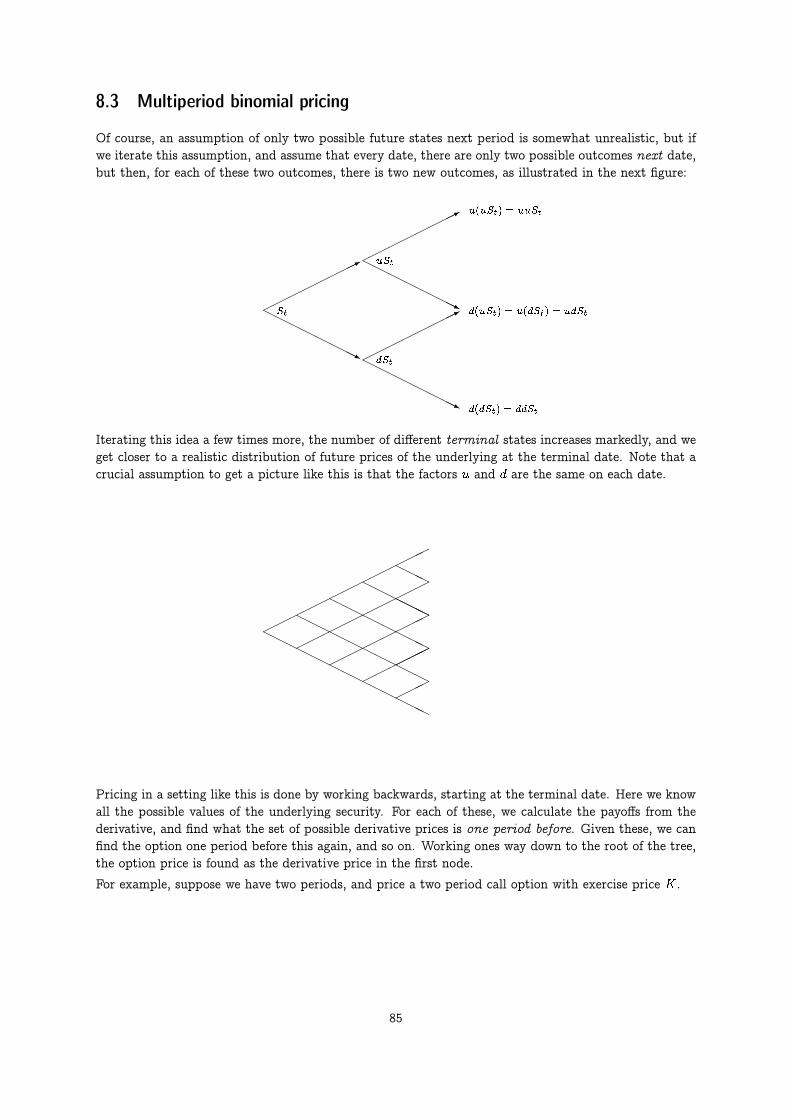
8.3 Multiperiod binomial pricing
Of course, an assumption of only two possible future states next period is somewhat unrealistic, but ifwe iterate this assumption, and assume that every date, there are only two possible outcomes next date,but then, for each of these two outcomes, there is two new outcomes, as illustrated in the next figure:
St���
���
��*
HHHHH
HHHj
uSt
dSt
���
���
��*
HHHHH
HHHj
���
���
��*
HHHHHH
HHj
u(uSt) = uuSt
d(uSt) = u(dSt) = udSt
d(dSt) = ddSt
Iterating this idea a few times more, the number of different terminal states increases markedly, and weget closer to a realistic distribution of future prices of the underlying at the terminal date. Note that acrucial assumption to get a picture like this is that the factors u and d are the same on each date.
�����
����
����
HHHHHH
HHHHHHH
HHHH
HHHHHH
���
���
����
HHHHH
HHH
����
����
HHHHH
�����
HHH
���
HHH
���
Pricing in a setting like this is done by working backwards, starting at the terminal date. Here we knowall the possible values of the underlying security. For each of these, we calculate the payoffs from thederivative, and find what the set of possible derivative prices is one period before. Given these, we canfind the option one period before this again, and so on. Working ones way down to the root of the tree,the option price is found as the derivative price in the first node.
For example, suppose we have two periods, and price a two period call option with exercise price K.
85

S0���
���
��*
HHHHH
HHHj
uS0
dS0
���
���
��*
HHHHH
HHHj
���
���
��*
HHHHH
HHHj
uuS0
udS0
ddS0
First step: Find terminal payoffs of derivative security:
���
�����*
HHHHH
HHHj
���
�����*
HHHHH
HHHj
���
���
��*
HHHHH
HHHj
Cuu = max(0; Suu �K)
Cdu = max(0; duS �K)
Cdd �max(0; ddS �K)
Next step: Find the two possible call prices at time 1:
Cu = e�r(qCuu + (1� q)Cud)
Cd = e�r(qCud + (1� q)Cdd)
C0���
��*
HHHHHj
Cu
Cd
Final step: Using the two possible payoffs at time 1, Cu and Cd, find option value at time 0:
C0 = e�r(qCu + (1� q)Cd)
Thus, binomial pricing really concerns “rolling backward” in a binomial tree, and programming thereforeconcerns an efficient way of traversing such a tree. The obvious data structure for describing such a treeis shown in C++ Code 8.2, where the value in each node is calculated from finding out the number of upand down steps are used to get to the particular node.
Exercise 8.2.
86

#include <vector>#include <cmath>using namespace std;
vector< vector<double> > binomial tree(const double& S0,const double& u,const double& d,const int& no steps){
vector< vector<double> > tree;for (int i=1;i<=no steps;++i){
vector<double> S(i);for (int j=0;j<i;++j){
S[j] = S0*pow(u,j)*pow(d,i�j�1);};tree.push back(S);
};return tree;
};
C++ Code 8.2: Building a binomial tree
In terms of computational efficiency the approcach of C++ Code 8.2 will not be optimal, since it requires alot of calls to the pow() functional call. More efficient would be to carry out the tree building by doing themultiplication from the previous node, for example the j’th vector is the j � 1’th vector times u, and thenone need to add one more node by multiplying the lowest element by d.
1. Implement such an alternative tree building procedure.
Basing the recursive calculation of a derivative price on a triangular array structure as shown inC++ Code 8.2 is the most natural approach, but with some cleverness based on understanding the structureof the binomial tree, we can get away with the more efficienent algorithm that is shown in C++ Code 8.3.Note that here we only use one vector<double>, not a triangular array as built above.
Example
Let S = 100:0, K = 100:0, r = 0:025, u = 1:05 and d = 1=u.
1. Price one and two period European Call options.
C++ program:
double S = 100.0; double K = 100.0; double r = 0.025;double u = 1.05; double d = 1/u;cout << " one period european call = "
<< option price call european binomial single period(S,K,r,u,d) << endl;int no periods = 2;cout << " two period european call = "
<< option price call european binomial multi period given ud(S,K,r,u,d,no periods) << endl;
Output from C++ program:
one period european call = 3.64342two period european call = 5.44255
Exercise 8.3.
Implement pricing of single and multi period binomial put options.
Further reading The derivation of the single period binomial is shown in for example Bossaerts andØdegaard (2001), Hull (2011) or McDonald (2013).
87
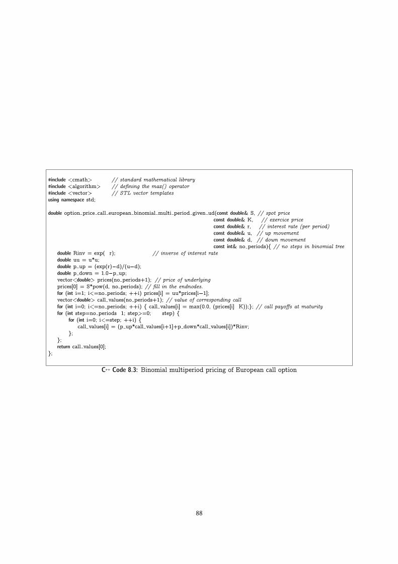
#include <cmath> // standard mathematical library#include <algorithm> // defining the max() operator#include <vector> // STL vector templatesusing namespace std;
double option price call european binomial multi period given ud(const double& S, // spot priceconst double& K, // exercice priceconst double& r, // interest rate (per period)const double& u, // up movementconst double& d, // down movementconst int& no periods){ // no steps in binomial tree
double Rinv = exp(�r); // inverse of interest ratedouble uu = u*u;double p up = (exp(r)�d)/(u�d);double p down = 1.0�p up;vector<double> prices(no periods+1); // price of underlyingprices[0] = S*pow(d, no periods); // fill in the endnodes.for (int i=1; i<=no periods; ++i) prices[i] = uu*prices[i�1];vector<double> call values(no periods+1); // value of corresponding callfor (int i=0; i<=no periods; ++i) { call values[i] = max(0.0, (prices[i]�K));}; // call payoffs at maturityfor (int step=no periods�1; step>=0; ��step) {
for (int i=0; i<=step; ++i) {call values[i] = (p up*call values[i+1]+p down*call values[i])*Rinv;
};};return call values[0];
};
C++ Code 8.3: Binomial multiperiod pricing of European call option
88

Chapter 9
Basic Option Pricing, the Black Scholesformula
Contents9.1 The formula . . . . . . . . . . . . . . . . . . . . . . . . . . . . . . . . . . . . . . . . . . . . 909.2 Understanding the why’s of the formula . . . . . . . . . . . . . . . . . . . . . . . . . . . . . . 92
9.2.1 The original Black Scholes analysis . . . . . . . . . . . . . . . . . . . . . . . . . 939.2.2 The limit of a binomial case . . . . . . . . . . . . . . . . . . . . . . . . . . . . . 939.2.3 The representative agent framework . . . . . . . . . . . . . . . . . . . . . . . . 93
9.3 Partial derivatives. . . . . . . . . . . . . . . . . . . . . . . . . . . . . . . . . . . . . . . . . 939.3.1 Delta . . . . . . . . . . . . . . . . . . . . . . . . . . . . . . . . . . . . . . . . . 939.3.2 Other Derivatives . . . . . . . . . . . . . . . . . . . . . . . . . . . . . . . . . . . 949.3.3 Implied Volatility. . . . . . . . . . . . . . . . . . . . . . . . . . . . . . . . . . . 96
9.4 References . . . . . . . . . . . . . . . . . . . . . . . . . . . . . . . . . . . . . . . . . . . . 98
The pricing of options and related instruments has been a major breakthrough for the use of financialtheory in practical application. Since the original papers of Black and Scholes (1973) and Merton (1973),there has been a wealth of practical and theoretical applications. We will now consider the orginal BlackScholes formula for pricing options, how it is calculated and used. For the basic intuition about optionpricing the reader should first read the discussion of the binomial model in the previous chapter, as thatis a much better environment for understanding what is actually calculated.
An option is a derivative security, its value depends on the value, or price, of some other underlyingsecurity, called the underlying security.. Let S denote the value, or price, of this underlying security.We need to keep track of what time this price is observed at, so let St denote that the price is observedat time t. A call (put) option gives the holder the right, but not the obligation, to buy (sell) someunderlying asset at a given price K, called the exercise price, on or before some given date T . If theoption is a so called European option, it can only be used (exercised) at the maturity date. If theoption is of the so called American type, it can be used (exercised) at any date up to and including thematurity date T . If exercised at time T , a call option provides payoff
CT = max(0; ST �K)
and a put option provides payoff
PT = max(0;K � ST )
The Black Scholes formulas provides analytical solutions for European put and call options, optionswhich can only be exercised at the options maturity date. Black and Scholes showed that the additional
89
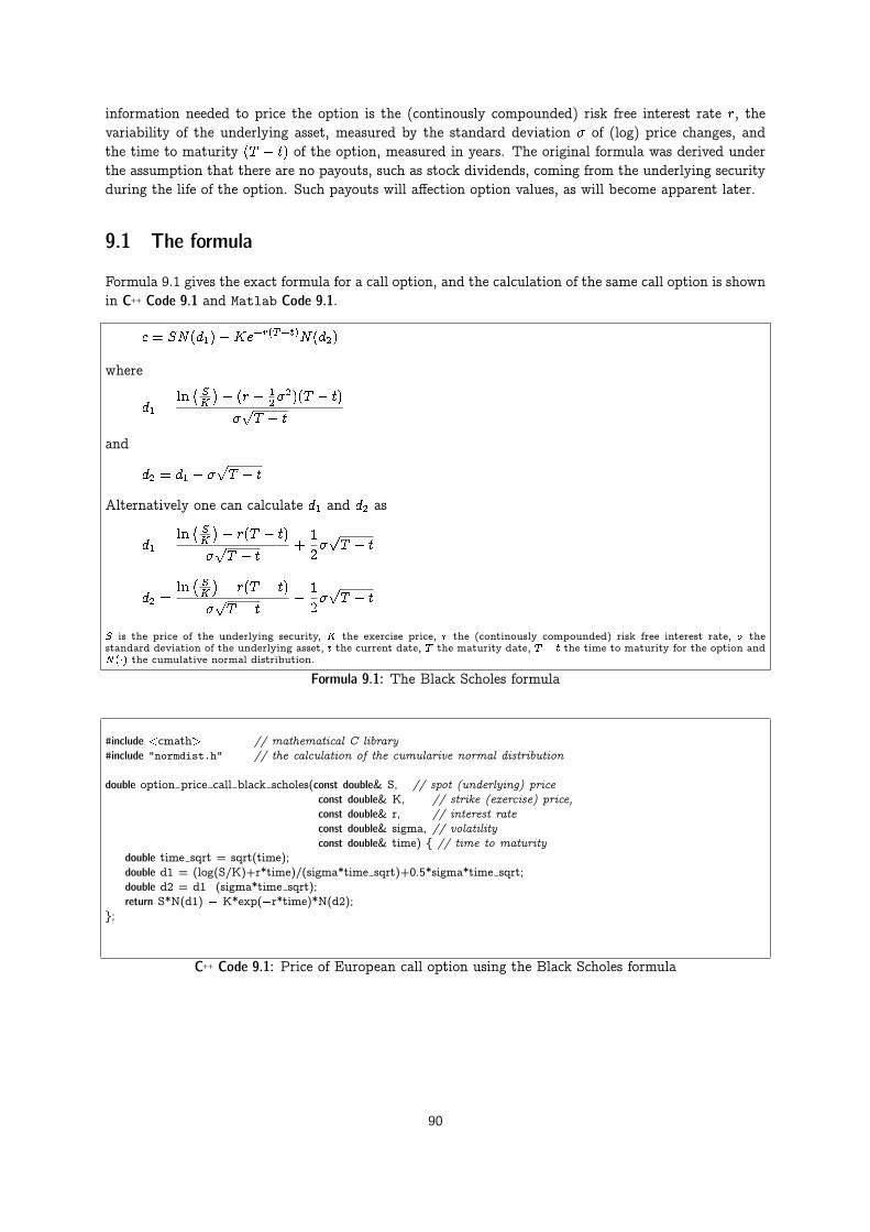
information needed to price the option is the (continously compounded) risk free interest rate r, thevariability of the underlying asset, measured by the standard deviation � of (log) price changes, andthe time to maturity (T � t) of the option, measured in years. The original formula was derived underthe assumption that there are no payouts, such as stock dividends, coming from the underlying securityduring the life of the option. Such payouts will affection option values, as will become apparent later.
9.1 The formula
Formula 9.1 gives the exact formula for a call option, and the calculation of the same call option is shownin C++ Code 9.1 and Matlab Code 9.1.
c = SN(d1)�Ke�r(T�t)N(d2)
where
d1 =ln�SK
�+ (r + 1
2�2)(T � t)
�pT � t
and
d2 = d1 � �pT � t
Alternatively one can calculate d1 and d2 as
d1 =ln�SK
�+ r(T � t)
�pT � t
+1
2�pT � t
d2 =ln�SK
�+ r(T � t)
�pT � t
� 1
2�pT � t
S is the price of the underlying security, K the exercise price, r the (continously compounded) risk free interest rate, � thestandard deviation of the underlying asset, t the current date, T the maturity date, T � t the time to maturity for the option andN(�) the cumulative normal distribution.
Formula 9.1: The Black Scholes formula
#include <cmath> // mathematical C library#include "normdist.h" // the calculation of the cumularive normal distribution
double option price call black scholes(const double& S, // spot (underlying) priceconst double& K, // strike (exercise) price,const double& r, // interest rateconst double& sigma, // volatilityconst double& time) { // time to maturity
double time sqrt = sqrt(time);double d1 = (log(S/K)+r*time)/(sigma*time sqrt)+0.5*sigma*time sqrt;double d2 = d1�(sigma*time sqrt);return S*N(d1) � K*exp(�r*time)*N(d2);
};
C++ Code 9.1: Price of European call option using the Black Scholes formula
90

function c = black scholes call(S,K,r,sigma,time)time sqrt = sqrt(time);d1 = (log(S/K)+r*time)/(sigma*time sqrt)+0.5*sigma*time sqrt;d2 = d1�(sigma*time sqrt);c = S * normcdf(d1) � K * exp(�r*time) * normcdf(d2);
endfunction
Matlab Code 9.1: Price of European call option using the Black Scholes formula
91
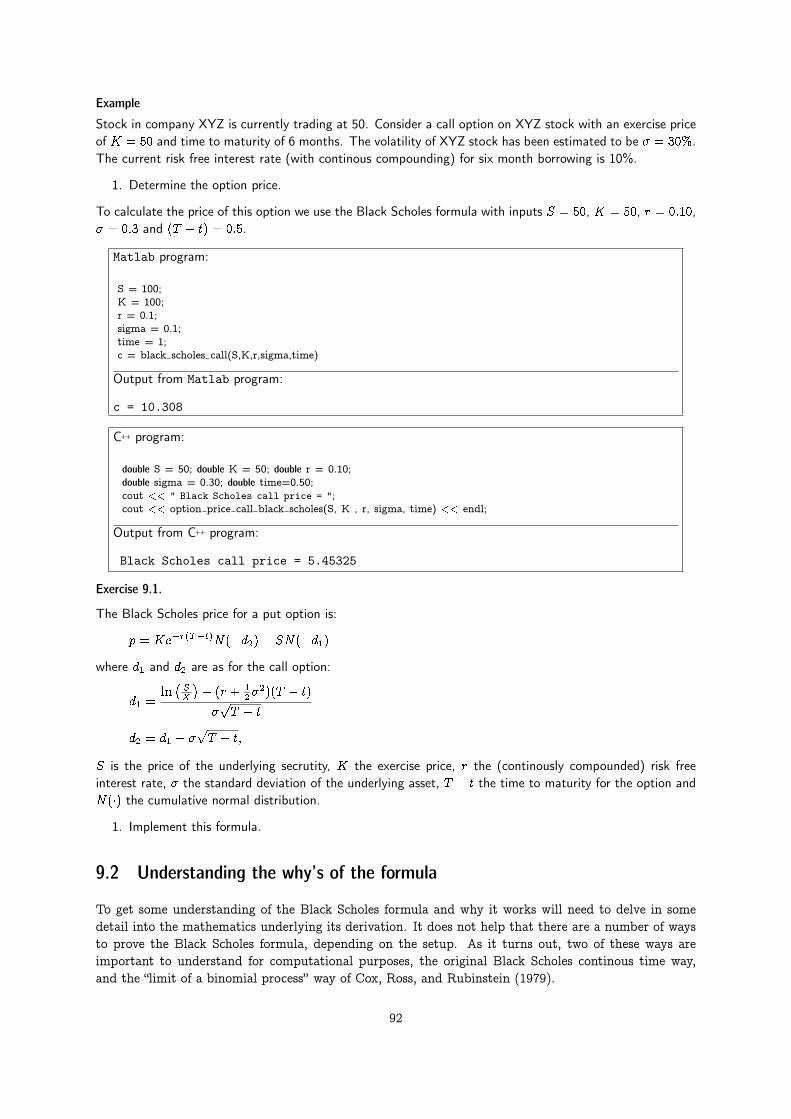
Example
Stock in company XYZ is currently trading at 50. Consider a call option on XYZ stock with an exercise priceof K = 50 and time to maturity of 6 months. The volatility of XYZ stock has been estimated to be � = 30%.The current risk free interest rate (with continous compounding) for six month borrowing is 10%.
1. Determine the option price.
To calculate the price of this option we use the Black Scholes formula with inputs S = 50, K = 50, r = 0:10,� = 0:3 and (T � t) = 0:5.
Matlab program:
S = 100;K = 100;r = 0.1;sigma = 0.1;time = 1;c = black scholes call(S,K,r,sigma,time)
Output from Matlab program:
c = 10.308
C++ program:
double S = 50; double K = 50; double r = 0.10;double sigma = 0.30; double time=0.50;cout << " Black Scholes call price = ";cout << option price call black scholes(S, K , r, sigma, time) << endl;
Output from C++ program:
Black Scholes call price = 5.45325
Exercise 9.1.
The Black Scholes price for a put option is:
p = Ke�r(T�t)N(�d2)� SN(�d1)where d1 and d2 are as for the call option:
d1 =ln�SX
�+ (r + 1
2�2)(T � t)
�pT � t
d2 = d1 � �pT � t;
S is the price of the underlying secrutity, K the exercise price, r the (continously compounded) risk freeinterest rate, � the standard deviation of the underlying asset, T � t the time to maturity for the option andN(�) the cumulative normal distribution.
1. Implement this formula.
9.2 Understanding the why’s of the formula
To get some understanding of the Black Scholes formula and why it works will need to delve in somedetail into the mathematics underlying its derivation. It does not help that there are a number of waysto prove the Black Scholes formula, depending on the setup. As it turns out, two of these ways areimportant to understand for computational purposes, the original Black Scholes continous time way,and the “limit of a binomial process” way of Cox, Ross, and Rubinstein (1979).
92

9.2.1 The original Black Scholes analysis
The primary assumption underlying the Black Scholes analyis concerns the stochastic process governingthe price of the underlying asset. The price of the underlying asset, S, is assumed to follow a geometricBrownian Motion process, conveniently written in either of the shorthand forms
dS = �Sdt+ �SdZ
or
dS
S= �dt+ �dZ
where � and � are constants, and Z is Brownian motion.
Using Ito’s lemma, the assumption of no arbitrage, and the ability to trade continuously, Black andScholes showed that the price of any contingent claim written on the underlying must solve the partialdifferential equation (9.1).
@f
@SrS +
@f
@t+
1
2
@2f
@S2�2S2 = rf (9.1)
For any particular contingent claim, the terms of the claim will give a number of boundary conditionsthat determines the form of the pricing formula.
The pde given in equation (9.1), with the boundary condition cT = max(0; ST �K) was shown by Blackand Scholes to have an analytical solution of functional form shown in the Black Scoles formula 9.1.
9.2.2 The limit of a binomial case
Another is to use the limit of a binomial process (Cox et al., 1979). The latter is particularly interesting,as it allows us to link the Black Scholes formula to the binomial, allowing the binomial framework to beused as an approximation.
9.2.3 The representative agent framework
A final way to show the BS formula to assume a representative agent and lognormality as was done inRubinstein (1976).
9.3 Partial derivatives.
In trading of options, a number of partial derivatives of the option price formula is important.
9.3.1 Delta
The first derivative of the option price with respect to the price of the underlying security is called thedelta of the option price. It is the derivative most people will run into, since it is important in hedgingof options.
@c
@S= N(d1)
C++ Code 9.2 shows the calculation of the delta for a call option.
93

#include <cmath>#include "normdist.h"
double option price delta call black scholes(const double& S, // spot priceconst double& K, // Strike (exercise) price,const double& r, // interest rateconst double& sigma, // volatilityconst double& time){ // time to maturity
double time sqrt = sqrt(time);double d1 = (log(S/K)+r*time)/(sigma*time sqrt) + 0.5*sigma*time sqrt;double delta = N(d1);return delta;
};
C++ Code 9.2: Calculating the delta of the Black Scholes call option price
9.3.2 Other Derivatives
The remaining derivatives are more seldom used, but all of them are relevant. All of them are listed informula 9.3.2.
Delta (�)
� =@c
@S= N(d1)
Gamma (�)
@2c
@S2=
n(d1)
S�pT � t
Theta (�) (careful about which of these you want)
@c
@(T � t)= Sn(d1)
1
2�
1pT � t
+ rKe�r(T�t)N(d2)
@c
@t= �Sn(d1)1
2�
1pT � t
� rKe�r(T�t)N(d2)
Vega
@c
@�= S
pT � tn(d1)
Rho (�)
@c
@r= K(T � t)e�r(T�t)N(d2)
S is the price of the underlying security, K the exercise price, r the (continously compounded) risk free interest rate, � thestandard deviation of the underlying asset, t the current date, T the maturity date and T � t the time to maturity for the option.
n(�) is the normal distribution function�n(z) = 1p
2�e�
12z2�
and N(�) the cumulative normal distribution�N(z) =
Rz
�1n(t)dt
�.
Formula 9.2: Partial derivatives of the Black Scholes call option formula
The calculation of all of these partial derivatives for a call option is shown in C++ Code 9.3.
Example
Consider again six month call options on XYZ stock. The option matures 6 months from now, at which timethe holder of the option can recive one unit of the underlying security by paying the exercise price of K = 50.The current price of the underlying security is S = 50. The volatility of the underlying security is given as� = 30%. The current risk free interest rate (with continous compounding) for six month borrowing is 10%.
94

#include <cmath>#include "normdist.h"using namespace std;
void option price partials call black scholes( const double& S, // spot priceconst double& K, // Strike (exercise) price,const double& r, // interest rateconst double& sigma, // volatilityconst double& time, // time to maturitydouble& Delta, // partial wrt Sdouble& Gamma, // second prt wrt Sdouble& Theta, // partial wrt timedouble& Vega, // partial wrt sigmadouble& Rho){ // partial wrt r
double time sqrt = sqrt(time);double d1 = (log(S/K)+r*time)/(sigma*time sqrt) + 0.5*sigma*time sqrt;double d2 = d1�(sigma*time sqrt);Delta = N(d1);Gamma = n(d1)/(S*sigma*time sqrt);Theta =� (S*sigma*n(d1))/(2*time sqrt) � r*K*exp( �r*time)*N(d2);Vega = S * time sqrt*n(d1);Rho = K*time*exp(�r*time)*N(d2);
};
C++ Code 9.3: Calculating the partial derivatives of a Black Scholes call option
1. Calculate the partial derivatives (Delta, Gamma, Theta, Vega and Rho) for this option.
To calculate the partial derivatives we use inputs S = 50, K = 50, r = 0:10, � = 0:3 and (T � t) = 0:5.
C++ program:
cout << " Black Scholes call partial derivatives " << endl;double S = 50; double K = 50; double r = 0.10;double sigma = 0.30; double time=0.50;double Delta, Gamma, Theta, Vega, Rho;option price partials call black scholes(S,K,r,sigma, time, Delta, Gamma, Theta, Vega, Rho);cout << " Delta = " << Delta << endl;cout << " Gamma = " << Gamma << endl;cout << " Theta = " << Theta << endl;cout << " Vega = " << Vega << endl;cout << " Rho = " << Rho << endl;
Output from C++ program:
Black Scholes call partial derivativesDelta = 0.633737Gamma = 0.0354789Theta = -6.61473Vega = 13.3046Rho = 13.1168
95

9.3.3 Implied Volatility.
In calculation of the option pricing formulas, in particular the Black Scholes formula, the only unknownis the standard deviation of the underlying stock. A common problem in option pricing is to find theimplied volatility, given the observed price quoted in the market. For example, given c0, the price of acall option, the following equation should be solved for the value of �:
c0 = c(S;K; r; �; T � t)
Unfortunately, this equation has no closed form solution, which means the equation must be numericallysolved to find �. What is probably the algorithmic simplest way to solve this is to use a binomial searchalgorithm, which is implemented in C++ Code 9.4. We start by bracketing the sigma by finding a highsigma that makes the BS price higher than the observed price, and then, given the bracketing interval,we search for the volatility in a systematic way. shows such a calculation.
#include <cmath>#include "fin_recipes.h"
double option price implied volatility call black scholes bisections(const double& S,const double& K,const double& r,const double& time,const double& option price){
if (option price<0.99*(S�K*exp(�time*r))) { // check for arbitrage violations.return 0.0; // Option price is too low if this happens
};
// simple binomial search for the implied volatility.// relies on the value of the option increasing in volatilityconst double ACCURACY = 1.0e�5; // make this smaller for higher accuracyconst int MAX ITERATIONS = 100;const double HIGH VALUE = 1e10;const double ERROR = �1e40;
// want to bracket sigma. first find a maximum sigma by finding a sigma// with a estimated price higher than the actual price.double sigma low=1e�5;double sigma high=0.3;double price = option price call black scholes(S,K,r,sigma high,time);while (price < option price) {
sigma high = 2.0 * sigma high; // keep doubling.price = option price call black scholes(S,K,r,sigma high,time);if (sigma high>HIGH VALUE) return ERROR; // panic, something wrong.
};for (int i=0;i<MAX ITERATIONS;i++){
double sigma = (sigma low+sigma high)*0.5;price = option price call black scholes(S,K,r,sigma,time);double test = (price�option price);if (fabs(test)<ACCURACY) { return sigma; };if (test < 0.0) { sigma low = sigma; }else { sigma high = sigma; }
};return ERROR;
};
C++ Code 9.4: Calculation of implied volatility of Black Scholes using bisections
Instead of this simple bracketing, which is actually pretty fast, and will (almost) always find the solution,we can use the Newton–Raphson formula for finding the root of an equation in a single variable. Thegeneral description of this method starts with a function f() for which we want to find a root.
f(x) = 0:
96

The function f() needs to be differentiable. Given a first guess x0, iterate by
xi+1 = xi � f(xi)
f 0(xi)
until
jf(xi)j < �
where � is the desired accuracy.1
In our case
f(x) = cobs � cBS(�)
and, each new iteration will calculate
�i+1 = �i +cobs � cBS(�i)
�@cBS()@�
C++ Code 9.5 shows the calculation of implied volatility using Newton-Raphson.
#include "fin_recipes.h"#include "normdist.h"#include <cmath>#include <iostream>double option price implied volatility call black scholes newton(const double& S,
const double& K,const double& r,const double& time,const double& option price) {
if (option price<0.99*(S�K*exp(�time*r))) { // check for arbitrage violations. Option price is too low if this happensreturn 0.0;
};
const int MAX ITERATIONS = 100;const double ACCURACY = 1.0e�5;double t sqrt = sqrt(time);
double sigma = (option price/S)/(0.398*t sqrt); // find initial valuefor (int i=0;i<MAX ITERATIONS;i++){
double price = option price call black scholes(S,K,r,sigma,time);double diff = option price �price;if (fabs(diff)<ACCURACY) return sigma;double d1 = (log(S/K)+r*time)/(sigma*t sqrt) + 0.5*sigma*t sqrt;double vega = S * t sqrt * n(d1);sigma = sigma + diff/vega;
};return �99e10; // something screwy happened, should throw exception
};
C++ Code 9.5: Calculation of implied volatility of Black Scholes using Newton-Raphson
Note that to use Newton-Raphson we need the derivative of the option price. For the Black-Scholesformula this is known, and we can use this. But for pricing formulas like the binomial, where the partialderivatives are not that easy to calculate, simple bisection is the preferred algorithm.
Example
Consider again six month call options on XYZ stock. The option matures 6 months from now, at which timethe holder of the option can recive one unit of the underlying security by paying the exercise price of K = 50.
1For further discussion of the Newton-Raphson formula and bracketing, a good source is chapter 9 of Press et al. (1992)
97

The current price of the underlying security is S = 50. The current risk free interest rate (with continouscompounding) for six month borrowing is 10%.
1. The current option price is C = 2:5. Determine the volatility implicit in this price.
The implied volatility is the � which, input in the Black Scholes formula with these other inputs, will producean option price of C = 2:5.
To calculate we use inputs S = 50, K = 50, r = 0:10 and (T � t) = 0:5.
C++ program:
double S = 50; double K = 50; double r = 0.10; double time=0.50;double C=2.5;cout << " Black Scholes implied volatility using Newton search = ";cout << option price implied volatility call black scholes newton(S,K,r,time,C) << endl;cout << " Black Scholes implied volatility using bisections = ";cout << option price implied volatility call black scholes bisections(S,K,r,time,C) << endl;
Output from C++ program:
Black Scholes implied volatility using Newton search = 0.0500427Black Scholes implied volatility using bisections = 0.0500419
9.4 References
Black and Scholes (1973) Merton (1973)
Gray and Gray (2001) has a simple proof of the formula.
98

Chapter 10
Warrants
Contents10.1 Warrant value in terms of assets . . . . . . . . . . . . . . . . . . . . . . . . . . . . . . . . . 9910.2 Valuing warrants when observing the stock value . . . . . . . . . . . . . . . . . . . . . . . . . 10010.3 Readings . . . . . . . . . . . . . . . . . . . . . . . . . . . . . . . . . . . . . . . . . . . . . 101
A warrant is an option-like security on equity, but it is issued by the same company which has issuedthe equity, and when a warrant is exercised, a new stock is issued. This new stock is issued at a thewarrant strike price, which is lower than the current stock price (If it wasn’t the warrant would not beexercised.) Since the new stock is a a fractional right to all cashflows, this stock issue waters out, ordilutes, the equity in a company. The degree of dilution is a function of how many warrants are issued.
10.1 Warrant value in terms of assets
Let K be the strike price, n the number of shares outstanding and m the number of warrants issued.Assume each warrant is for 1 new share, and let At be the current asset value of firm. Suppose allwarrants are exercised simultaneously. Then the assets of the firm increase by the number of warrantstimes the strike price of the warrant.
At +mK;
but this new asset value is spread over more shares, since each exercised warrant is now an equity. Theassets of the firm is spread over all shares, hence each new share is worth:
At +mK
m+ n
making each exercised warrant worth:
At +mK
m+ n�K =
n
m+ n
�At
n�K
�If we knew the current value of assets in the company, we could value the warrant in two steps:
1. Value the option using the Black Scholes formula and At
n as the current stock price.
2. Multiply the resulting call price with nm+n .
If we let Wt be the warrant value, the above arguments are summarized as:
Wt =n
n+mCBS
�A
n;K; �; r; (T � t)
�;
99

where CBS(�) is the Black Scholes formula.
10.2 Valuing warrants when observing the stock value
However, one does not necessarily observe the asset value of the firm. Typically one only observes theequity value of the firm. If we let St be the current stock price, the asset value is really:
At = nSt +mWt
Using the stock price, one would value the warrant as
Wt =n
n+mCBS
�nSt +mWt
n;K; �; r; (T � t)
�or
Wt =n
n+mCBS
�St +
m
nWt;K; �; r; (T � t)
�Note that this gives the value of Wt as a function of Wt. One need to solve this equation numerically tofind Wt.
The numerical solution for Wt is done using the Newton-Rhapson method. Let
g(Wt) = Wt � n
n+mCBS
�St +
m
nWt;K; �; r; (T � t)
�Starting with an initial guess for the warrant value W o
t , the Newton-Rhapson method is that one iteratesas follows
W it = W i�1
t � g(W i�1t )
g0(W i�1t )
;
where i signifies iteration i, until the criterion function g(W i�1t ) is below some given accuracy �. In this
case
g0(Wt) = 1� m
m+ nN(d1)
where
d1 =ln�St+
mnWt
K
�+ (r + 1
2�2)(T � t)
�pT � t
An obvious starting value is to set calculate the Black Scholes value using the current stock price, andmultiply it with m
m+n .
C++ Code 10.1 implements this calculation.
Example
A stock is currently priced at S = 48. Consider warrants on the same company with exercise price K = 40 andtime to maturity of six months. The company has n = 10000 shares outstanding, and has issued m = 1000
warrants. The current (continously compounded) risk free interest rate is 8%. Determine the current warrantprice.
100

#include "fin_recipes.h"#include "normdist.h"#include <cmath>
const double EPSILON=0.00001;
double warrant price adjusted black scholes(const double& S,const double& K,const double& r,const double& sigma,const double& time,const double& m, // number of warrants outstandingconst double& n){ // number of shares outstanding
double time sqrt = sqrt(time);double w = (n/(n+m))*option price call black scholes(S,K,r,sigma,time);double g = w�(n/(n+m))*option price call black scholes(S+(m/n)*w,K,r,sigma,time);while (fabs(g)>EPSILON) {
double d1 = (log((S+(m/n))/K)+r*time)/(sigma*time sqrt)+0.5*sigma*time sqrt;double gprime = 1�(m/n)*N(d1);w=w�g/gprime;g = w�(n/(n+m))*option price call black scholes(S+(m/n)*w,K,r,sigma,time);
};return w;
};
C++ Code 10.1: Adjusted Black Scholes value for a Warrant
C++ program:
double S = 48; double K = 40; double r = 0.08; double sigma = 0.30;double time = 0.5; double m = 1000; double n = 10000;double w = warrant price adjusted black scholes(S,K,r,sigma, time, m, n);cout << " warrant price = " << w << endl;
Output from C++ program:
warrant price = 10.142
Exercise 10.1.
The solution method assumes that all warrants are exercised simultanously. Can you see where this assumptionis used?
10.3 Readings
McDonald (2013) and Hull (2011) are general references. A problem with warrants is that exercise of allwarrants simultaneously is not necessarily optimal.
Press et al. (1992) discusses the Newton-Rhapson method for root finding.
101
Chapter 11
Extending the Black Scholes formula
Contents11.1 Adjusting for payouts of the underlying. . . . . . . . . . . . . . . . . . . . . . . . . . . . . . . 102
11.1.1 Continous Payouts from underlying. . . . . . . . . . . . . . . . . . . . . . . . . 10211.1.2 Dividends. . . . . . . . . . . . . . . . . . . . . . . . . . . . . . . . . . . . . . . . 103
11.2 American options . . . . . . . . . . . . . . . . . . . . . . . . . . . . . . . . . . . . . . . . . 10411.2.1 Exact american call formula when stock is paying one dividend. . . . . . . . . 105
11.3 Options on futures . . . . . . . . . . . . . . . . . . . . . . . . . . . . . . . . . . . . . . . . 10811.3.1 Black’s model . . . . . . . . . . . . . . . . . . . . . . . . . . . . . . . . . . . . . 108
11.4 Foreign Currency Options . . . . . . . . . . . . . . . . . . . . . . . . . . . . . . . . . . . . . 10911.5 Perpetual puts and calls . . . . . . . . . . . . . . . . . . . . . . . . . . . . . . . . . . . . . . 11011.6 Readings . . . . . . . . . . . . . . . . . . . . . . . . . . . . . . . . . . . . . . . . . . . . . 111
11.1 Adjusting for payouts of the underlying.
For options on other financial instruments than stocks, we have to allow for the fact that the underlyingmay have payouts during the life of the option. For example, in working with commodity options, thereis often some storage costs if one wanted to hedge the option by buying the underlying.
11.1.1 Continous Payouts from underlying.
The simplest case is when the payouts are done continuously. To value an European option, a simpleadjustment to the Black Scholes formula is all that is needed. Let q be the continuous payout of theunderlying commodity.
Call and put prices for European options are then given by formula 11.1, which are implemented inC++ Code 11.1.
Exercise 11.1.
The price of a put on an underlying security with a continous payout of q is:
p = Ke�r(T�t)N(�d2)� Se�q(T�t)N(�d1)
1. Implement this formula.
102
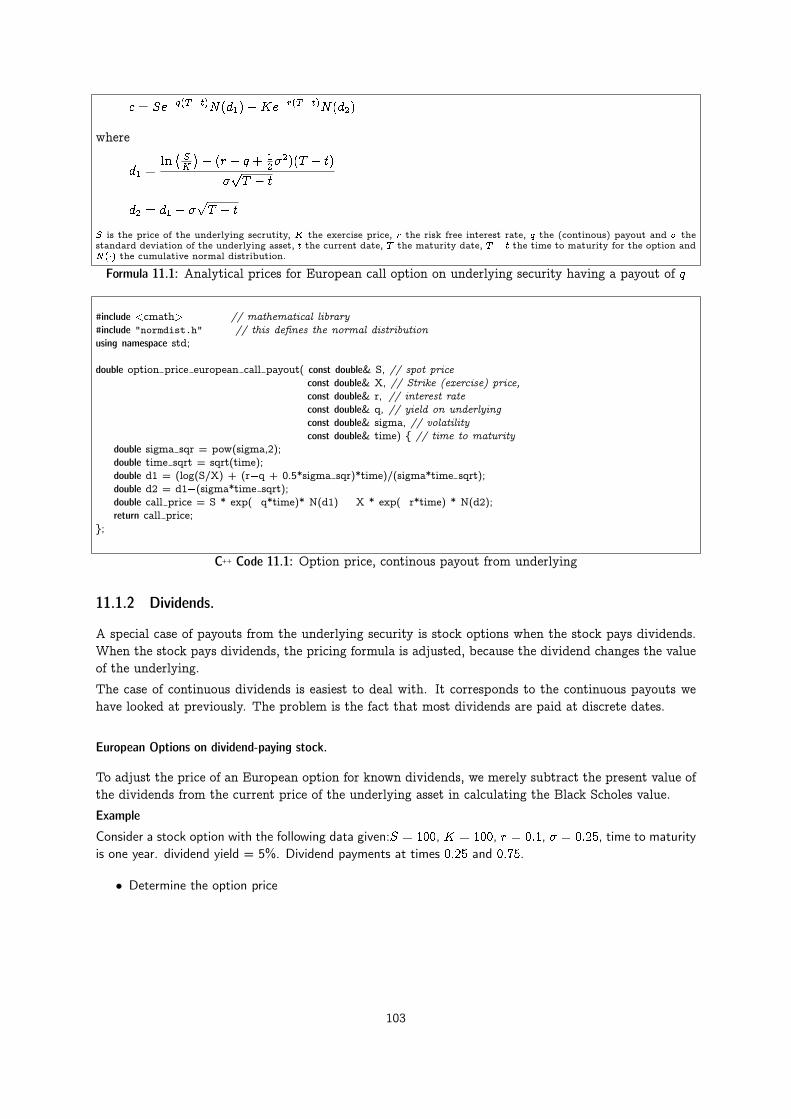
c = Se�q(T�t)N(d1)�Ke�r(T�t)N(d2)
where
d1 =ln�SK
�+ (r � q + 1
2�2)(T � t)
�pT � t
d2 = d1 � �pT � t
S is the price of the underlying secrutity, K the exercise price, r the risk free interest rate, q the (continous) payout and � thestandard deviation of the underlying asset, t the current date, T the maturity date, T � t the time to maturity for the option andN(�) the cumulative normal distribution.
Formula 11.1: Analytical prices for European call option on underlying security having a payout of q
#include <cmath> // mathematical library#include "normdist.h" // this defines the normal distributionusing namespace std;
double option price european call payout( const double& S, // spot priceconst double& X, // Strike (exercise) price,const double& r, // interest rateconst double& q, // yield on underlyingconst double& sigma, // volatilityconst double& time) { // time to maturity
double sigma sqr = pow(sigma,2);double time sqrt = sqrt(time);double d1 = (log(S/X) + (r�q + 0.5*sigma sqr)*time)/(sigma*time sqrt);double d2 = d1�(sigma*time sqrt);double call price = S * exp(�q*time)* N(d1) � X * exp(�r*time) * N(d2);return call price;
};
C++ Code 11.1: Option price, continous payout from underlying
11.1.2 Dividends.
A special case of payouts from the underlying security is stock options when the stock pays dividends.When the stock pays dividends, the pricing formula is adjusted, because the dividend changes the valueof the underlying.
The case of continuous dividends is easiest to deal with. It corresponds to the continuous payouts wehave looked at previously. The problem is the fact that most dividends are paid at discrete dates.
European Options on dividend-paying stock.
To adjust the price of an European option for known dividends, we merely subtract the present value ofthe dividends from the current price of the underlying asset in calculating the Black Scholes value.
Example
Consider a stock option with the following data given:S = 100, K = 100, r = 0:1, � = 0:25, time to maturityis one year. dividend yield = 5%. Dividend payments at times 0:25 and 0:75.
• Determine the option price
103

#include <cmath> // mathematical library#include <vector>#include "fin_recipes.h" // define the black scholes price
double option price european call dividends( const double& S,const double& K,const double& r,const double& sigma,const double& time to maturity,const vector<double>& dividend times,const vector<double>& dividend amounts ) {
double adjusted S = S;for (int i=0;i<dividend times.size();i++) {
if (dividend times[i]<=time to maturity){adjusted S �= dividend amounts[i] * exp(�r*dividend times[i]);
};};return option price call black scholes(adjusted S,K,r,sigma,time to maturity);
};
C++ Code 11.2: European option price, dividend paying stock
C++ program:
double S = 100.0; double K = 100.0;double r = 0.1; double sigma = 0.25;double time=1.0;double dividend yield=0.05;vector<double> dividend times; vector<double> dividend amounts;dividend times.push back(0.25); dividend amounts.push back(2.5);dividend times.push back(0.75); dividend amounts.push back(2.5);cout << " european stock call option with contininous dividend = "
<< option price european call payout(S,K,r,dividend yield,sigma,time) << endl;cout << " european stock call option with discrete dividend = "
<< option price european call dividends(S,K,r,sigma,time,dividend times,dividend amounts) << endl;
Output from C++ program:
european stock call option with contininous dividend = 11.7344european stock call option with discrete dividend = 11.8094
11.2 American options
American options are much harder to deal with than European ones. The problem is that it may beoptimal to use (exercise) the option before the final expiry date. This optimal exercise policy will affectthe value of the option, and the exercise policy needs to be known when solving the pde. However, theexercise policy is not known. There is therefore no general analytical solutions for American call andput options. There are some special cases. For American call options on assets that do not have anypayouts, the American call price is the same as the European one, since the optimal exercise policy isto not exercise. For American puts this this not the case, it may pay to exercise them early. Whenthe underlying asset has payouts, it may also pay to exercise an American call option early. There isone known known analytical price for American call options, which is the case of a call on a stock thatpays a known dividend once during the life of the option, which is discussed next. In all other casesthe American price has to be approximated using one of the techniques discussed in later chapters:Binomial approximation, numerical solution of the partial differential equation, or another numericalapproximation.
104

11.2.1 Exact american call formula when stock is paying one dividend.
When a stock pays dividend, a call option on the stock may be optimally exercised just before the stockgoes ex-dividend. While the general dividend problem is usually approximated somehow, for the specialcase of one dividend payment during the life of an option an analytical solution is available, due toRoll–Geske–Whaley.
If we let S be the stock price, K the exercise price, D1 the amount of dividend paid, t1 the time ofdividend payment, T the maturity date of option, we denote the time to dividend payment �1 = T � t1and the time to maturity � = T � t.
A first check of early exercise is:
D1 � K�1� e�r(T�t1)
�If this inequality is fulfilled, early exercise is not optimal, and the value of the option is
c(S � e�r(t1�t)D1;K; r; �; (T � t))
where c(�) is the regular Black Scholes formula.
If the inequality is not fulfilled, one performs the calculation shown in Formula 11.2 and implemented inC++ Code 11.3.
C = (S �D1e�r(t1�t)) (N(b1) +N(a1;�b1; �)) +Ke�r(T�t))N(a2;�b2; �)� (K �D1)e
�r(t1�t)N(b2)
where
� = �r
(t1 � t
T � t
a1 =ln�S�D1e
�q(�1K
�+ (r + 1
2�2)�
�p�
a2 = a1 � �pT � t
b1 =ln�S�D1e
�r(t1�t)
�S
�+ (r + 1
2�2)(t1 � t)
�p(t1 � t)
b2 = b1 � �pT � t
and �S solves
c( �S; t1) = �S +D1 �K
S is the price of the underlying secrutity, K the exercise price, r the risk free interest rate, D1 is the dividend amount and � thestandard deviation of the underlying asset, t the current date, T the maturity date, T � t the time to maturity for the optionand N(�) the cumulative normal distribution. N() with one argument is the univariate normal cumulative distribution. N() withthree arguments is the bivariate normal distribution with the correlation between the two normals given as the third arguement.
Formula 11.2: Roll–Geske–Whaley price of american call option paying one fixed dividend
Example
Consider an option on a stock paying one dividend. The relevant data is S = 100, K = 100;r=0.1, � = 0:25,� = 1:0, �1 = 0:5 and D1 = 10.Price the option.
105
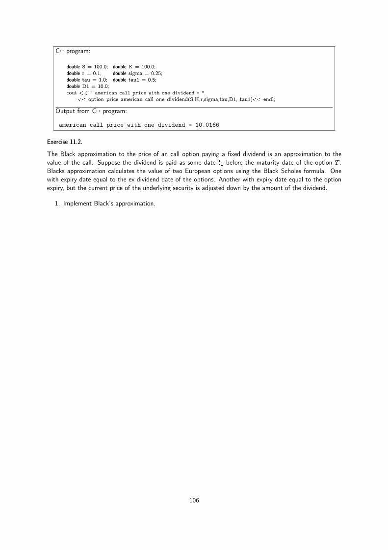
C++ program:
double S = 100.0; double K = 100.0;double r = 0.1; double sigma = 0.25;double tau = 1.0; double tau1 = 0.5;double D1 = 10.0;cout << " american call price with one dividend = "
<< option price american call one dividend(S,K,r,sigma,tau,D1, tau1)<< endl;
Output from C++ program:
american call price with one dividend = 10.0166
Exercise 11.2.
The Black approximation to the price of an call option paying a fixed dividend is an approximation to thevalue of the call. Suppose the dividend is paid as some date t1 before the maturity date of the option T .Blacks approximation calculates the value of two European options using the Black Scholes formula. Onewith expiry date equal to the ex dividend date of the options. Another with expiry date equal to the optionexpiry, but the current price of the underlying security is adjusted down by the amount of the dividend.
1. Implement Black’s approximation.
106

#include <cmath>#include "normdist.h" // define the normal distribution functions#include "fin_recipes.h" // the regular black sholes formula
double option price american call one dividend(const double& S,const double& K,const double& r,const double& sigma,const double& tau,const double& D1,const double& tau1){
if (D1 <= K* (1.0�exp(�r*(tau�tau1)))) // check for no exercisereturn option price call black scholes(S�exp(�r*tau1)*D1,K,r,sigma,tau);
const double ACCURACY = 1e�6; // decrease this for more accuracydouble sigma sqr = sigma*sigma;double tau sqrt = sqrt(tau);double tau1 sqrt = sqrt(tau1);double rho = � sqrt(tau1/tau);
double S bar = 0; // first find the S bar that solves c=S bar+D1-Kdouble S low=0; // the simplest: binomial searchdouble S high=S; // start by finding a very high S above S bardouble c = option price call black scholes(S high,K,r,sigma,tau�tau1);double test = c�S high�D1+K;while ( (test>0.0) && (S high<=1e10) ) {
S high *= 2.0;c = option price call black scholes(S high,K,r,sigma,tau�tau1);test = c�S high�D1+K;
};if (S high>1e10) { // early exercise never optimal, find BS value
return option price call black scholes(S�D1*exp(�r*tau1),K,r,sigma,tau);};S bar = 0.5 * S high; // now find S bar that solves c=S bar-D+Kc = option price call black scholes(S bar,K,r,sigma,tau�tau1);test = c�S bar�D1+K;while ( (fabs(test)>ACCURACY) && ((S high�S low)>ACCURACY) ) {
if (test<0.0) { S high = S bar; }else { S low = S bar; };S bar = 0.5 * (S high + S low);c = option price call black scholes(S bar,K,r,sigma,tau�tau1);test = c�S bar�D1+K;
};double a1 = (log((S�D1*exp(�r*tau1))/K) +( r+0.5*sigma sqr)*tau) / (sigma*tau sqrt);double a2 = a1 � sigma*tau sqrt;double b1 = (log((S�D1*exp(�r*tau1))/S bar)+(r+0.5*sigma sqr)*tau1)/(sigma*tau1 sqrt);double b2 = b1 � sigma * tau1 sqrt;double C = (S�D1*exp(�r*tau1)) * N(b1) + (S�D1*exp(�r*tau1)) * N(a1,�b1,rho)
� (K*exp(�r*tau))*N(a2,�b2,rho) � (K�D1)*exp(�r*tau1)*N(b2);return C;
};
C++ Code 11.3: Option price, Roll–Geske–Whaley call formula for dividend paying stock
107

11.3 Options on futures
11.3.1 Black’s model
For an European option written on a futures contract, we use an adjustment of the Black Scholes solution,which was developed in Black (1976). Essentially we replace S0 with e�r(T�t)rF in the Black Scholesformula, and get the formula shown in 11.3 and implemented in C++ Code 11.4.
c = e�r(T�t) (FN(d1)�KN(d2))
where
d1 =ln�FK
�+ 1
2�2(T � t)
�pT � t
d2 = d1 � �pT � t
F is the futures price, K is the exercise price, r the risk free interest rate, � the volatility of the futuresprice, and T � t is the time to maturity of the option (in years).Formula 11.3: Black’s formula for the price of an European Call option with a futures contract as theunderlying security
#include <cmath> // mathematics library#include "normdist.h" // normal distributionusing namespace std;
double futures option price call european black( const double& F, // futures priceconst double& K, // exercise priceconst double& r, // interest rateconst double& sigma, // volatilityconst double& time){ // time to maturity
double sigma sqr = sigma*sigma;double time sqrt = sqrt(time);double d1 = (log (F/K) + 0.5 * sigma sqr * time) / (sigma * time sqrt);double d2 = d1 � sigma * time sqrt;return exp(�r*time)*(F * N(d1) � K * N(d2));
};
C++ Code 11.4: Price of European Call option on Futures contract
Example
Price a futures option in the Black setting. Information: F = 50, K = 45, r = 8%, � = 0:2, and time tomaturity is a half year.
C++ program:
double F = 50.0; double K = 45.0;double r = 0.08; double sigma = 0.2;double time=0.5;cout << " european futures call option = "
<< futures option price put european black(F,K,r,sigma,time) << endl;
Output from C++ program:
european futures call option = 0.851476
Exercise 11.3.
108

The Black formula for a put option on a futures contract is
p = e�r(T�t) (KN(�d2)� FN(�d1))
where the varibles are as defined for the call option.
1. Implement the put option price.
11.4 Foreign Currency Options
Another relatively simple adjustment of the Black Scholes formula occurs when the underlying securityis a currency exchange rate (spot rate). In this case one adjusts the Black-Scholes equation for theinterest-rate differential.
Let S be the spot exchange rate, and now let r be the domestic interest rate and rf the foreign interestrate. � is then the volatility of changes in the exchange rate. The calculation of the price of an Europeancall option is then shown in formula 11.4 and implented in C++ Code 11.5.
c = Se�rf (T�t)N(d1)�Ke�r(T�t)N(d2)
where
d1 =ln�SK
�+�r � rf +
12�
2�(T � t)
�pT � t
d2 = d1 � �pT � t
S is the spot exchange rate and K the exercise price. r is the domestic interest rate and rf the foreign interest rate. � is thevolatility of changes in the exchange rate. T � t is the time to maturity for the option.
Formula 11.4: European currency call
#include <cmath>#include "normdist.h" // define the normal distribution function
double currency option price call european( const double& S, // exchange rate,const double& X, // exercise,const double& r, // r domestic,const double& r f, // r foreign,const double& sigma, // volatility,const double& time){ // time to maturity
double sigma sqr = sigma*sigma;double time sqrt = sqrt(time);double d1 = (log(S/X) + (r�r f+ (0.5*sigma sqr)) * time)/(sigma*time sqrt);double d2 = d1 � sigma * time sqrt;return S * exp(�r f*time) * N(d1) � X * exp(�r*time) * N(d2);
};
C++ Code 11.5: European Futures Call option on currency
Example
Price a European currency call given the following information S = 50, K = 52, r = 8%, rf = 5%, � = 20%
and time to maturity = 0.5 years.
109
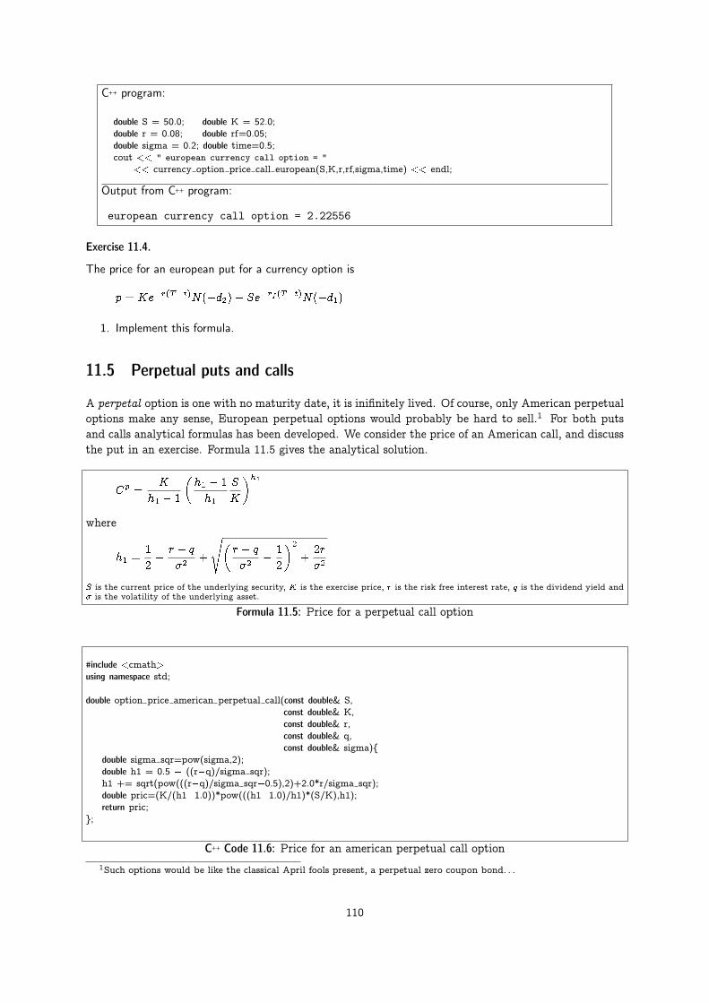
C++ program:
double S = 50.0; double K = 52.0;double r = 0.08; double rf=0.05;double sigma = 0.2; double time=0.5;cout << " european currency call option = "
<< currency option price call european(S,K,r,rf,sigma,time) << endl;
Output from C++ program:
european currency call option = 2.22556
Exercise 11.4.
The price for an european put for a currency option is
p = Ke�r(T�t)N(�d2)� Se�rf (T�t)N(�d1)
1. Implement this formula.
11.5 Perpetual puts and calls
A perpetal option is one with no maturity date, it is inifinitely lived. Of course, only American perpetualoptions make any sense, European perpetual options would probably be hard to sell.1 For both putsand calls analytical formulas has been developed. We consider the price of an American call, and discussthe put in an exercise. Formula 11.5 gives the analytical solution.
Cp =K
h1 � 1
�h1 � 1
h1
S
K
�h1where
h1 =1
2� r � q
�2+
s�r � q
�2� 1
2
�2
+2r
�2
S is the current price of the underlying security, K is the exercise price, r is the risk free interest rate, q is the dividend yield and� is the volatility of the underlying asset.
Formula 11.5: Price for a perpetual call option
#include <cmath>using namespace std;
double option price american perpetual call(const double& S,const double& K,const double& r,const double& q,const double& sigma){
double sigma sqr=pow(sigma,2);double h1 = 0.5 � ((r�q)/sigma sqr);h1 += sqrt(pow(((r�q)/sigma sqr�0.5),2)+2.0*r/sigma sqr);double pric=(K/(h1�1.0))*pow(((h1�1.0)/h1)*(S/K),h1);return pric;
};
C++ Code 11.6: Price for an american perpetual call option1Such options would be like the classical April fools present, a perpetual zero coupon bond. . .
110

Example
Price a perpetual call, given the following informtation S = 50:0;K = 40:0; r = 0:05; q = 0:02; � = 0:05
C++ program:
double S=50.0; double K=40.0;double r=0.05; double q=0.02;double sigma=0.05;double price = option price american perpetual call(S,K,r,q,sigma);cout << " perpetual call price = " << price << endl;
Output from C++ program:
perpetual call price = 19.4767
Exercise 11.5.
The price for a perpetual american put is
P p =K
1� h2
�h2 � 1
h2
S
K
�h2where
h2 =1
2� r � q
�2�s�
r � q
�2� 1
2
�2
+2r
�2
1. Implement the calculation of this formula.
11.6 Readings
Hull (2011) and McDonald (2013) are general references. A first formulation of an analytical call pricewith dividends was in Roll (1977b). This had some errors, that were partially corrected in Geske (1979),before Whaley (1981) gave a final, correct formula. See Hull (2011) for a textbook summary. Black(1976) is the original development of the futures option. The original formulations of European foreigncurrency option prices are in Garman and Kohlhagen (1983) and Grabbe (1983). The price of a perpetualput was first shown in Merton (1973). For a perpetual call see McDonald and Siegel (1986). The notationfor perpetual puts and calls follows the summary in (McDonald, 2013, pg. 393).
111

Chapter 12
Option pricing with binomial approximations
Contents12.1 Introduction . . . . . . . . . . . . . . . . . . . . . . . . . . . . . . . . . . . . . . . . . . . . 11212.2 Pricing of options in the Black Scholes setting . . . . . . . . . . . . . . . . . . . . . . . . . . 113
12.2.1 European Options . . . . . . . . . . . . . . . . . . . . . . . . . . . . . . . . . . 11412.2.2 American Options . . . . . . . . . . . . . . . . . . . . . . . . . . . . . . . . . . 11412.2.3 Matlab implementation . . . . . . . . . . . . . . . . . . . . . . . . . . . . . . . 116
12.3 How good is the binomial approximation? . . . . . . . . . . . . . . . . . . . . . . . . . . . . . 11912.3.1 Estimating partials. . . . . . . . . . . . . . . . . . . . . . . . . . . . . . . . . . 120
12.4 Adjusting for payouts for the underlying . . . . . . . . . . . . . . . . . . . . . . . . . . . . . 12312.5 Pricing options on stocks paying dividends using a binomial approximation . . . . . . . . . . . . 124
12.5.1 Checking for early exercise in the binomial model. . . . . . . . . . . . . . . . . 12412.5.2 Proportional dividends. . . . . . . . . . . . . . . . . . . . . . . . . . . . . . . . 12412.5.3 Discrete dividends . . . . . . . . . . . . . . . . . . . . . . . . . . . . . . . . . . 126
12.6 Option on futures . . . . . . . . . . . . . . . . . . . . . . . . . . . . . . . . . . . . . . . . . 12812.7 Foreign Currency options . . . . . . . . . . . . . . . . . . . . . . . . . . . . . . . . . . . . . 13012.8 References . . . . . . . . . . . . . . . . . . . . . . . . . . . . . . . . . . . . . . . . . . . . 131
12.1 Introduction
We have shown binomial calculations given an up and down movement in chapter 8. However, binomialoption pricing can also be viewed as an approximation to a continuous time distribution by judiciouschoice of the constants u and d. To do so one has to ask: Is it possible to find a parametrization (choiceof u and d) of a binomial process
112
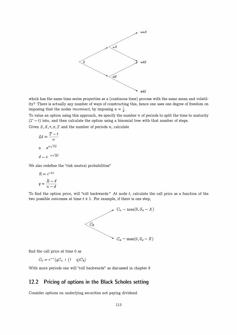
S���
�����*
HHHHH
HHHj
uS
dS
���
���
��*
HHHHH
HHHj
���
���
��*
HHHHHH
HHj
uuS
udS
ddS
which has the same time series properties as a (continous time) process with the same mean and volatil-ity? There is actually any number of ways of constructing this, hence one uses one degree of freedom onimposing that the nodes reconnect, by imposing u = 1
d .
To value an option using this approach, we specify the number n of periods to split the time to maturity(T � t) into, and then calculate the option using a binomial tree with that number of steps.
Given S;X; r; �; T and the number of periods n, calculate
�t =T � t
n
u = e�p�t
d = e��p�t
We also redefine the “risk neutral probabilities”
R = er�t
q =R� d
u� d
To find the option price, will “roll backwards:” At node t, calculate the call price as a function of thetwo possible outcomes at time t+ 1. For example, if there is one step,
C0���
���
��*
HHHHH
HHHj
Cu = max(0; Su �X)
Cd = max(0; Sd �X)
find the call price at time 0 as
C0 = e�r(qCu + (1� q)Cd)
With more periods one will “roll backwards” as discussed in chapter 8
12.2 Pricing of options in the Black Scholes setting
Consider options on underlying securities not paying dividend.
113

12.2.1 European Options
For European options, binomial trees are not that much used, since the Black Scholes model will givethe correct answer, but it is useful to see the construction of the binomial tree without the checks forearly exercise, which is the American case.
The computer algorithm for a binomial in the following merits some comments. There is only one vectorof call prices, and one may think one needs two, one at time t and another at time t+ 1. (Try to writedown the way you would solve it before looking at the algorithm below.) But by using the fact that thebranches reconnect, it is possible to get away with the algorithm below, using one less array. You maywant to check how this works. It is also a useful way to make sure one understands binomial optionpricing.
#include <cmath> // standard mathematical library#include <algorithm> // defining the max() operator#include <vector> // STL vector templatesusing namespace std;
double option price call european binomial( const double& S, // spot priceconst double& K, // exercice priceconst double& r, // interest rateconst double& sigma, // volatilityconst double& t, // time to maturityconst int& steps){ // no steps in binomial tree
double R = exp(r*(t/steps)); // interest rate for each stepdouble Rinv = 1.0/R; // inverse of interest ratedouble u = exp(sigma*sqrt(t/steps)); // up movementdouble uu = u*u;double d = 1.0/u;double p up = (R�d)/(u�d);double p down = 1.0�p up;vector<double> prices(steps+1); // price of underlyingprices[0] = S*pow(d, steps); // fill in the endnodes.for (int i=1; i<=steps; ++i) prices[i] = uu*prices[i�1];vector<double> call values(steps+1); // value of corresponding callfor (int i=0; i<=steps; ++i) call values[i] = max(0.0, (prices[i]�K)); // call payoffs at maturityfor (int step=steps�1; step>=0; ��step) {
for (int i=0; i<=step; ++i) {call values[i] = (p up*call values[i+1]+p down*call values[i])*Rinv;
};};return call values[0];
};
C++ Code 12.1: Option price for binomial european
12.2.2 American Options
An American option differs from an European option by the exercise possibility. An American optioncan be exercised at any time up to the maturity date, unlike the European option, which can only beexercised at maturity. In general, there is unfortunately no analytical solution to the American optionproblem, but in some cases it can be found. For example, for an American call option on non-dividendpaying stock, the American price is the same as the European call.
It is in the case of American options, allowing for the possibility of early exercise, that binomial approx-imations are useful. At each node we calculate the value of the option as a function of the next periodsprices, and then check for the value exercising of exercising the option now
C++ Code 12.2 illustrates the calculation of the price of an American call.
114
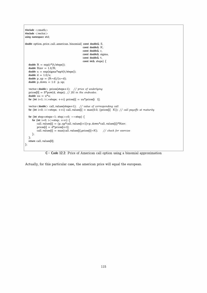
#include <cmath>#include <vector>using namespace std;
double option price call american binomial( const double& S,const double& K,const double& r,const double& sigma,const double& t,const int& steps) {
double R = exp(r*(t/steps));double Rinv = 1.0/R;double u = exp(sigma*sqrt(t/steps));double d = 1.0/u;double p up = (R�d)/(u�d);double p down = 1.0�p up;
vector<double> prices(steps+1); // price of underlyingprices[0] = S*pow(d, steps); // fill in the endnodes.double uu = u*u;for (int i=1; i<=steps; ++i) prices[i] = uu*prices[i�1];
vector<double> call values(steps+1); // value of corresponding callfor (int i=0; i<=steps; ++i) call values[i] = max(0.0, (prices[i]�K)); // call payoffs at maturity
for (int step=steps�1; step>=0; ��step) {for (int i=0; i<=step; ++i) {
call values[i] = (p up*call values[i+1]+p down*call values[i])*Rinv;prices[i] = d*prices[i+1];call values[i] = max(call values[i],prices[i]�K); // check for exercise
};};return call values[0];
};
C++ Code 12.2: Price of American call option using a binomial approximation
Actually, for this particular case, the american price will equal the european.
115

12.2.3 Matlab implementation
To illustrate differences between Matlab and C++, consider the two implementations in Matlab Code 12.1and Matlab Code 12.2. The calculation of a put is more compact, with less loops, by some judicious useof array indexing.
function c = bin am call( S, K, r, sigma,t,steps)R = exp(r*(t/steps));Rinv = 1.0/R;u = exp(sigma*sqrt(t/steps));d = 1.0/u;p up = (R�d)/(u�d);p down = 1.0�p up;prices = zeros(steps+1);
prices(1) = S*(d^steps);uu = u*u;for i=2:steps
prices(i) = uu*prices(i�1);end
call values = max(0.0, (prices�K));for step=steps:�1:1
for i=1:step+1call values(i) = (p up*call values(i+1)+p down*call values(i))*Rinv;prices(i) = d*prices(i+1);call values(i) = max(call values(i),prices(i)�K);
endendc= call values(1);
end
Matlab Code 12.1: Price of American call using a binomial approximation
116

function p = bin am put( S, K, r, sigma, t, steps)R = exp(r*(t/steps));Rinv = 1.0/R;u = exp(sigma*sqrt(t/steps));d = 1.0/u;p up = (R�d)/(u�d);p down = 1.0�p up;
prices = zeros(steps+1,1);prices(1) = S*(d^steps);uu = u*u;for i=2:steps+1prices(i) = uu*prices(i�1);
endvalues = max(0.0, (K�prices));for step=steps:�1:1
values = Rinv * ( p up*values(2:step+1) + p down*values(1:step) );prices = u*prices(1:step);values = max(values,K�prices);
endp=values(1);
end
Matlab Code 12.2: Price of American put using a binomial approximation
117
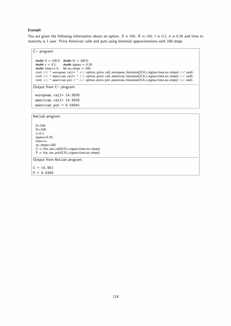
Example
You are given the following information about an option: S = 100, K = 100, r = 0:1, � = 0:25 and time tomaturity is 1 year. Price American calls and puts using binomial approximations with 100 steps.
C++ program:
double S = 100.0; double K = 100.0;double r = 0.1; double sigma = 0.25;double time=1.0; int no steps = 100;cout << " european call= " << option price call european binomial(S,K,r,sigma,time,no steps) << endl;cout << " american call= " << option price call american binomial(S,K,r,sigma,time,no steps) << endl;cout << " american put = " << option price put american binomial(S,K,r,sigma,time,no steps) << endl;
Output from C++ program:
european call= 14.9505american call= 14.9505american put = 6.54691
Matlab program:
S=100;K=100;r=0.1;sigma=0.25;time=1;no steps=100;C = bin am call(S,K,r,sigma,time,no steps)P = bin am put(S,K,r,sigma,time,no steps)
Output from Matlab program:
C = 14.951P = 6.5469
118
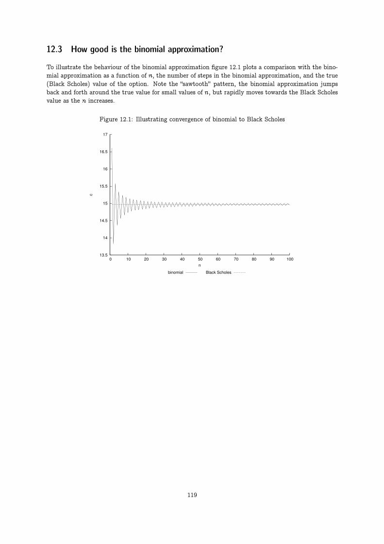
12.3 How good is the binomial approximation?
To illustrate the behaviour of the binomial approximation figure 12.1 plots a comparison with the bino-mial approximation as a function of n, the number of steps in the binomial approximation, and the true(Black Scholes) value of the option. Note the “sawtooth” pattern, the binomial approximation jumpsback and forth around the true value for small values of n, but rapidly moves towards the Black Scholesvalue as the n increases.
Figure 12.1: Illustrating convergence of binomial to Black Scholes
13.5
14
14.5
15
15.5
16
16.5
17
0 10 20 30 40 50 60 70 80 90 100
c
n
binomial Black Scholes
119

12.3.1 Estimating partials.
It is always necessary to calculate the partial derivatives as well as the option price. Let us start withDelta, the derivative of the option price with respect to the underlying. The binomial methods gives usways to approximate these as well. How to find them in the binomial case are described in Hull (2011).The implementation in C++ Code 12.3 is for the non–dividend case.
#include <cmath>#include <algorithm>#include <vector>using namespace std;
double option price delta american call binomial(const double& S,const double& K,const double& r,const double& sigma,const double& t,const int& no steps){ // steps in binomial
double R = exp(r*(t/no steps));double Rinv = 1.0/R;double u = exp(sigma*sqrt(t/no steps));double d = 1.0/u;double uu= u*u;double pUp = (R�d)/(u�d);double pDown = 1.0 � pUp;
vector<double> prices (no steps+1);prices[0] = S*pow(d, no steps);for (int i=1; i<=no steps; ++i) prices[i] = uu*prices[i�1];
vector<double> call values (no steps+1);for (int i=0; i<=no steps; ++i) call values[i] = max(0.0, (prices[i]�K));
for (int CurrStep=no steps�1 ; CurrStep>=1; ��CurrStep) {for (int i=0; i<=CurrStep; ++i) {
prices[i] = d*prices[i+1];call values[i] = (pDown*call values[i]+pUp*call values[i+1])*Rinv;call values[i] = max(call values[i], prices[i]�K); // check for exercise
};};double delta = (call values[1]�call values[0])/(S*u�S*d);return delta;
};
C++ Code 12.3: Delta
Calculation of all the derivatives are shown in C++ Code 12.4
120

#include <cmath>#include <algorithm>#include "fin_recipes.h"
void option price partials american call binomial(const double& S, // spot priceconst double& K, // Exercise price,const double& r, // interest rateconst double& sigma, // volatilityconst double& time, // time to maturityconst int& no steps, // steps in binomialdouble& delta, // partial wrt Sdouble& gamma, // second prt wrt Sdouble& theta, // partial wrt timedouble& vega, // partial wrt sigmadouble& rho){ // partial wrt r
vector<double> prices(no steps+1);vector<double> call values(no steps+1);double delta t =(time/no steps);double R = exp(r*delta t);double Rinv = 1.0/R;double u = exp(sigma*sqrt(delta t));double d = 1.0/u;double uu= u*u;double pUp = (R�d)/(u�d);double pDown = 1.0 � pUp;prices[0] = S*pow(d, no steps);for (int i=1; i<=no steps; ++i) prices[i] = uu*prices[i�1];for (int i=0; i<=no steps; ++i) call values[i] = max(0.0, (prices[i]�K));for (int CurrStep=no steps�1; CurrStep>=2; ��CurrStep) {
for (int i=0; i<=CurrStep; ++i) {prices[i] = d*prices[i+1];call values[i] = (pDown*call values[i]+pUp*call values[i+1])*Rinv;call values[i] = max(call values[i], prices[i]�K); // check for exercise
};};double f22 = call values[2];double f21 = call values[1];double f20 = call values[0];for (int i=0;i<=1;i++) {
prices[i] = d*prices[i+1];call values[i] = (pDown*call values[i]+pUp*call values[i+1])*Rinv;call values[i] = max(call values[i], prices[i]�K); // check for exercise
};double f11 = call values[1];double f10 = call values[0];prices[0] = d*prices[1];call values[0] = (pDown*call values[0]+pUp*call values[1])*Rinv;call values[0] = max(call values[0], S�K); // check for exercise on first datedouble f00 = call values[0];delta = (f11�f10)/(S*u�S*d);double h = 0.5 * S * ( uu � d*d);gamma = ( (f22�f21)/(S*(uu�1)) � (f21�f20)/(S*(1�d*d)) ) / h;theta = (f21�f00) / (2*delta t);double diff = 0.02;double tmp sigma = sigma+diff;double tmp prices = option price call american binomial(S,K,r,tmp sigma,time,no steps);vega = (tmp prices�f00)/diff;diff = 0.05;double tmp r = r+diff;tmp prices = option price call american binomial(S,K,tmp r,sigma,time,no steps);rho = (tmp prices�f00)/diff;
};
C++ Code 12.4: Hedge parameters
121

Example
Given the following information: S = 100, K = 100, r = 0:1, � = 0:25 and time to maturity is 1 year, Use100 steps in the binomial approximation.
1. Estimate all the “greeks” for the option: delta(�), gamma, theta, vega and rho.
C++ program:
double S = 100.0; double K = 100.0;double r = 0.1; double sigma = 0.25;double time=1.0; int no steps = 100;double delta, gamma, theta, vega, rho;option price partials american call binomial(S,K,r, sigma, time, no steps,
delta, gamma, theta, vega, rho);cout << " Call price partials " << endl;cout << " delta = " << delta << endl;cout << " gamma = " << gamma << endl;cout << " theta = " << theta << endl;cout << " vega = " << vega << endl;cout << " rho = " << rho << endl;
Output from C++ program:
Call price partialsdelta = 0.699792gamma = 0.0140407theta = -9.89067vega = 34.8536rho = 56.9652
Exercise 12.1.
Consider an American call option on non-dividend paying stock, where S = 100, K = 100, � = 0:2,(T � t) = 1 and r = 0:1.
1. Calculate the price of this option using Black Scholes
2. Calculate the price using a binomial approximation, using 10, 100 and 1000 steps in the approximation.
3. Discuss sources of differences in the estimated prices.
122

12.4 Adjusting for payouts for the underlying
The simplest case of a payout is the similar one to the one we saw in the Black Scholes case, a continouspayout of y. This y needs to be brought into the binomial framework. Here we use it to adjust theprobability:
�t =p(T � t)=n
u = e��t
d =1
u
pu =e(r�y)�t � d
u� d
pd = 1� pu
For example, the last node
C0 = e�r�t(puCu + (1� pu)Cd)
#include <cmath> // standard mathematical library#include <algorithm> // defines the max() operator#include <vector> // STL vector templatesusing namespace std;
double option price call american binomial( const double& S, // spot priceconst double& K, // exercice priceconst double& r, // interest rateconst double& y, // continous payoutconst double& sigma, // volatilityconst double& t, // time to maturityconst int& steps) { // no steps in binomial tree
double R = exp(r*(t/steps)); // interest rate for each stepdouble Rinv = 1.0/R; // inverse of interest ratedouble u = exp(sigma*sqrt(t/steps)); // up movementdouble uu = u*u;double d = 1.0/u;double p up = (exp((r�y)*(t/steps))�d)/(u�d);double p down = 1.0�p up;vector<double> prices(steps+1); // price of underlyingprices[0] = S*pow(d, steps);for (int i=1; i<=steps; ++i) prices[i] = uu*prices[i�1]; // fill in the endnodes.
vector<double> call values(steps+1); // value of corresponding callfor (int i=0; i<=steps; ++i) call values[i] = max(0.0, (prices[i]�K)); // call payoffs at maturity
for (int step=steps�1; step>=0; ��step) {for (int i=0; i<=step; ++i) {
call values[i] = (p up*call values[i+1]+p down*call values[i])*Rinv;prices[i] = d*prices[i+1];call values[i] = max(call values[i],prices[i]�K); // check for exercise
};};return call values[0];
};
C++ Code 12.5: Binomial option price with continous payout
123
12.5 Pricing options on stocks paying dividends using a binomial approximation
12.5.1 Checking for early exercise in the binomial model.
If the underlying asset is a stock paying dividends during the maturity of the option, the terms of theoption is not adjusted to reflect this cash payment, which means that the option value will reflect thedividend payments.
In the binomial model, the adjustment for dividends depend on whether the dividends are discrete orproportional.
12.5.2 Proportional dividends.
For proportional dividends, we simply multiply with an adjustment factor the stock prices at the ex–dividend date, the nodes in the binomial tree will “link up” again, and we can use the same “rolling back”procedure.
124

#include <cmath>#include <algorithm>#include <vector>#include "fin_recipes.h"#include <iostream>
double option price call american proportional dividends binomial(const double& S,const double& K,const double& r,const double& sigma,const double& time,const int& no steps,const vector<double>& dividend times,const vector<double>& dividend yields) {
// note that the last dividend date should be before the expiry date, problems if dividend at terminal nodeint no dividends = int(dividend times.size());if (no dividends == 0) {
return option price call american binomial(S,K,r,sigma,time,no steps); // price w/o dividends};double delta t = time/no steps;double R = exp(r*delta t);double Rinv = 1.0/R;double u = exp(sigma*sqrt(delta t));double uu= u*u;double d = 1.0/u;double pUp = (R�d)/(u�d);double pDown = 1.0 � pUp;vector<int> dividend steps(no dividends); // when dividends are paidfor (int i=0; i<no dividends; ++i) {
dividend steps[i] = (int)(dividend times[i]/time*no steps);};vector<double> prices(no steps+1);vector<double> call prices(no steps+1);prices[0] = S*pow(d, no steps); // adjust downward terminal prices by dividendsfor (int i=0; i<no dividends; ++i) { prices[0]*=(1.0�dividend yields[i]); };for (int i=1; i<=no steps; ++i) { prices[i] = uu*prices[i�1]; };for (int i=0; i<=no steps; ++i) call prices[i] = max(0.0, (prices[i]�K));
for (int step=no steps�1; step>=0; ��step) {for (int i=0;i<no dividends;++i) { // check whether dividend paid
if (step==dividend steps[i]) {for (int j=0;j<=(step+1);++j) {
prices[j]*=(1.0/(1.0�dividend yields[i]));};
};};for (int i=0; i<=step; ++i) {
call prices[i] = (pDown*call prices[i]+pUp*call prices[i+1])*Rinv;prices[i] = d*prices[i+1];call prices[i] = max(call prices[i], prices[i]�K); // check for exercise
};};return call prices[0];
};
C++ Code 12.6: Binomial option price of stock option where stock pays proportional dividends
125

12.5.3 Discrete dividends
The problem is when the dividends are constant dollar amounts. In that case the nodes of the binomialtree do not “link up,” and the number of branches increases dramatically, which means that the time todo the calculation is increased.
The algorithm presented in C++ Code 12.7 implements this case, with no linkup, by constructing a bi-nomial tree up to the ex-dividend date, and then, at the terminal nodes of that tree, call itself withone less dividend payment, and time to maturity the time remaining at the ex-dividend date. Doingthat calculates the value of the option at the ex-dividend date, which is then compared to the value ofexercising just before the ex-dividend date. It is a instructive example of using recursion in simplifyingcalculations, but as with most recursive solutions, it has a cost in computing time. For large binomialtrees and several dividends this procedure is costly in computing time.
126

#include <cmath>#include <vector>#include "fin_recipes.h"#include <iostream>double option price call american discrete dividends binomial(const double& S,
const double& K,const double& r,const double& sigma,const double& t,const int& steps,const vector<double>& dividend times,const vector<double>& dividend amounts) {
int no dividends = int(dividend times.size());if (no dividends==0) return option price call american binomial(S,K,r,sigma,t,steps);// just do regularint steps before dividend = (int)(dividend times[0]/t*steps);const double R = exp(r*(t/steps));const double Rinv = 1.0/R;const double u = exp(sigma*sqrt(t/steps));const double d = 1.0/u;const double pUp = (R�d)/(u�d);const double pDown = 1.0 � pUp;double dividend amount = dividend amounts[0];vector<double> tmp dividend times(no dividends�1); // temporaries withvector<double> tmp dividend amounts(no dividends�1); // one less dividendfor (int i=0;i<(no dividends�1);++i){
tmp dividend amounts[i] = dividend amounts[i+1];tmp dividend times[i] = dividend times[i+1] � dividend times[0];
};vector<double> prices(steps before dividend+1);vector<double> call values(steps before dividend+1);prices[0] = S*pow(d, steps before dividend);for (int i=1; i<=steps before dividend; ++i) prices[i] = u*u*prices[i�1];for (int i=0; i<=steps before dividend; ++i){
double value alive= option price call american discrete dividends binomial(prices[i]�dividend amount,K, r, sigma,
t�dividend times[0],// time after first dividendsteps�steps before dividend,tmp dividend times,tmp dividend amounts);
call values[i] = max(value alive,(prices[i]�K)); // compare to exercising now};for (int step=steps before dividend�1; step>=0; ��step) {
for (int i=0; i<=step; ++i) {prices[i] = d*prices[i+1];call values[i] = (pDown*call values[i]+pUp*call values[i+1])*Rinv;call values[i] = max(call values[i], prices[i]�K);
};};return call values[0];
};
C++ Code 12.7: Binomial option price of stock option where stock pays discrete dividends
127

Example
Given the following information S = 100, K = 100, r = 0:1, � = 0:25 and time to maturity is 1 year,Calculate option price with two different assumptions about dividends:
1. Continuous payout d = 0:02.
2. Discrete payout, d = 0:025 at times 0:25 and 0:75.
C++ program:
double S = 100.0; double K = 100.0;double r = 0.10; double sigma = 0.25;double time=1.0;int no steps = 100;double d=0.02;cout << " call price with continuous dividend payout = "
<< option price call american binomial(S,K,r,d,sigma,time,no steps) << endl;vector<double> dividend times; vector<double> dividend yields;dividend times.push back(0.25); dividend yields.push back(0.025);dividend times.push back(0.75); dividend yields.push back(0.025);cout << " call price with proportial dividend yields at discrete dates = "
<< option price call american proportional dividends binomial(S,K,r,sigma,time,no steps,dividend times, dividend yields)
<< endl;vector<double> dividend amounts; dividend amounts.push back(2.5); dividend amounts.push back(2.5);cout << " call price with proportial dividend amounts at discrete dates = "
<< option price call american discrete dividends binomial(S,K,r,sigma,time,no steps,dividend times, dividend amounts)
<< endl;
Output from C++ program:
call price with continuous dividend payout = 13.5926call price with proportial dividend yields at discrete dates = 11.8604call price with proportial dividend amounts at discrete dates = 12.0233
12.6 Option on futures
For American options, because of the feasibility of early exercise, the binomial model is used to approx-imate the option value for both puts and calls.
Example
F = 50:0;K = 45:0; r = 0:08; sigma = 0:2, time=0.5, no steps=100; Price the futures option
C++ program:
double F = 50.0; double K = 45.0;double r = 0.08; double sigma = 0.2;double time=0.5;int no steps=100;cout << " european futures call option = "
<< futures option price call american binomial(F,K,r,sigma,time,no steps) << endl;
Output from C++ program:
european futures call option = 5.74254
128
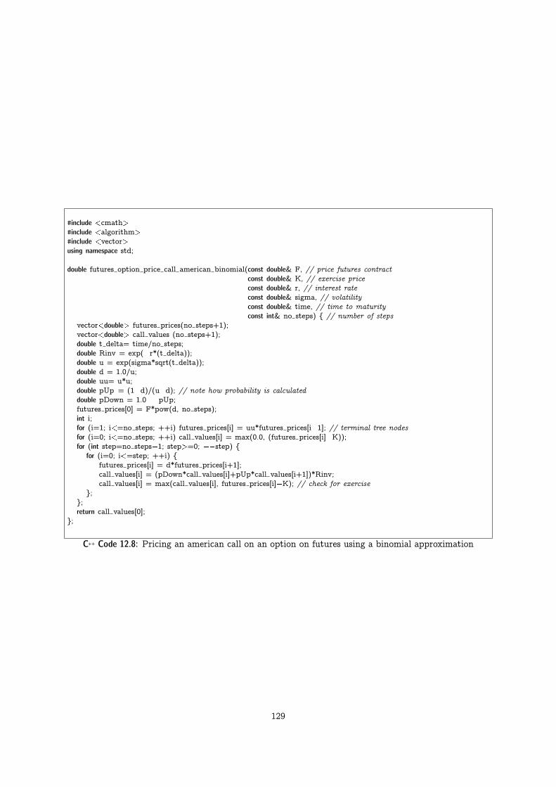
#include <cmath>#include <algorithm>#include <vector>using namespace std;
double futures option price call american binomial(const double& F, // price futures contractconst double& K, // exercise priceconst double& r, // interest rateconst double& sigma, // volatilityconst double& time, // time to maturityconst int& no steps) { // number of steps
vector<double> futures prices(no steps+1);vector<double> call values (no steps+1);double t delta= time/no steps;double Rinv = exp(�r*(t delta));double u = exp(sigma*sqrt(t delta));double d = 1.0/u;double uu= u*u;double pUp = (1�d)/(u�d); // note how probability is calculateddouble pDown = 1.0 � pUp;futures prices[0] = F*pow(d, no steps);int i;for (i=1; i<=no steps; ++i) futures prices[i] = uu*futures prices[i�1]; // terminal tree nodesfor (i=0; i<=no steps; ++i) call values[i] = max(0.0, (futures prices[i]�K));for (int step=no steps�1; step>=0; ��step) {
for (i=0; i<=step; ++i) {futures prices[i] = d*futures prices[i+1];call values[i] = (pDown*call values[i]+pUp*call values[i+1])*Rinv;call values[i] = max(call values[i], futures prices[i]�K); // check for exercise
};};return call values[0];
};
C++ Code 12.8: Pricing an american call on an option on futures using a binomial approximation
129

12.7 Foreign Currency options
For American options, the usual method is approximation using binomial trees, checking for early exercisedue to the interest rate differential.
#include <cmath>#include <algorithm>#include <vector>using namespace std;
double currency option price call american binomial(const double& S,const double& K,const double& r,const double& r f,const double& sigma,const double& time,const int& no steps) {
vector<double> exchange rates(no steps+1);vector<double> call values(no steps+1);double t delta= time/no steps;double Rinv = exp(�r*(t delta));double u = exp(sigma*sqrt(t delta));double d = 1.0/u;double uu= u*u;double pUp = (exp((r�r f)*t delta)�d)/(u�d); // adjust for foreign int.ratedouble pDown = 1.0 � pUp;exchange rates[0] = S*pow(d, no steps);int i;for (i=1; i<=no steps; ++i) {
exchange rates[i] = uu*exchange rates[i�1]; // terminal tree nodes}for (i=0; i<=no steps; ++i) call values[i] = max(0.0, (exchange rates[i]�K));for (int step=no steps�1; step>=0; ��step) {
for (i=0; i<=step; ++i) {exchange rates[i] = d*exchange rates[i+1];call values[i] = (pDown*call values[i]+pUp*call values[i+1])*Rinv;call values[i] = max(call values[i], exchange rates[i]�K); // check for exercise
};};return call values[0];
};
C++ Code 12.9: Pricing an american call on an option on currency using a binomial approximation
Example
Price a futures currency option with the following information: S = 50;K = 52; r = 0:08; rf = 0:05; � = 0:2,time=0.5, number of steps = 100.
C++ program:
double S = 50.0; double K = 52.0;double r = 0.08; double rf=0.05;double sigma = 0.2; double time=0.5;int no steps = 100;cout << " european currency option call = "
<< currency option price call american binomial(S,K,r,rf,sigma,time,no steps) << endl;
Output from C++ program:
european currency option call = 2.23129
130

12.8 References
The original source for binomial option pricing was the paper by Cox et al. (1979). Textbook discussionsare in Cox and Rubinstein (1985), Bossaerts and Ødegaard (2001) and Hull (2011).
131
Chapter 13
Finite Differences
Contents13.1 Explicit Finite differences . . . . . . . . . . . . . . . . . . . . . . . . . . . . . . . . . . . . . 13213.2 European Options. . . . . . . . . . . . . . . . . . . . . . . . . . . . . . . . . . . . . . . . . 13213.3 American Options. . . . . . . . . . . . . . . . . . . . . . . . . . . . . . . . . . . . . . . . . 13413.4 Implicit finite differences . . . . . . . . . . . . . . . . . . . . . . . . . . . . . . . . . . . . . 13713.5 An example matrix class . . . . . . . . . . . . . . . . . . . . . . . . . . . . . . . . . . . . . 13713.6 Finite Differences . . . . . . . . . . . . . . . . . . . . . . . . . . . . . . . . . . . . . . . . . 13713.7 American Options . . . . . . . . . . . . . . . . . . . . . . . . . . . . . . . . . . . . . . . . . 13713.8 European Options . . . . . . . . . . . . . . . . . . . . . . . . . . . . . . . . . . . . . . . . . 14013.9 References . . . . . . . . . . . . . . . . . . . . . . . . . . . . . . . . . . . . . . . . . . . . 141
13.1 Explicit Finite differences
The method of choice for any engineer given a differential equation to solve is to numerically approximateit using a finite difference scheme, which is to approximate the continous differential equation with adiscrete difference equation, and solve this difference equation.
13.2 European Options.
For European options we do not need to use the finite difference scheme, but we show how one would findthe european price for comparison purposes. We show the case of an explicit finite difference scheme inC++ Code 13.1. A problem with the explicit version is that it may not converge for certain combinationsof inputs.
132

#include <cmath>#include <vector>using namespace std;
double option price put european finite diff explicit(const double& S,const double& X,const double& r,const double& sigma,const double& time,const int& no S steps,const int& no t steps) {
double sigma sqr = pow(sigma,2);int M=no S steps; if ((no S steps%2)==1) { ++M; } // need no S steps to be even:double delta S = 2.0*S/M;vector<double> S values(M+1);for (unsigned m=0;m<=M;m++) { S values[m] = m*delta S; };int N=no t steps;double delta t = time/N;
vector<double> a(M);vector<double> b(M);vector<double> c(M);double r1=1.0/(1.0+r*delta t);double r2=delta t/(1.0+r*delta t);for (unsigned int j=1;j<M;j++){
a[j] = r2*0.5*j*(�r+sigma sqr*j);b[j] = r1*(1.0�sigma sqr*j*j*delta t);c[j] = r2*0.5*j*(r+sigma sqr*j);
};vector<double> f next(M+1);for (unsigned m=0;m<=M;++m) { f next[m]=max(0.0,X�S values[m]); };double f[M+1];for (int t=N�1;t>=0;��t) {
f[0]=X;for (unsigned m=1;m<M;++m) {
f[m]=a[m]*f next[m�1]+b[m]*f next[m]+c[m]*f next[m+1];};f[M] = 0;for (unsigned m=0;m<=M;++m) { f next[m] = f[m]; };
};return f[M/2];
};
C++ Code 13.1: Explicit finite differences calculation of european put option
133
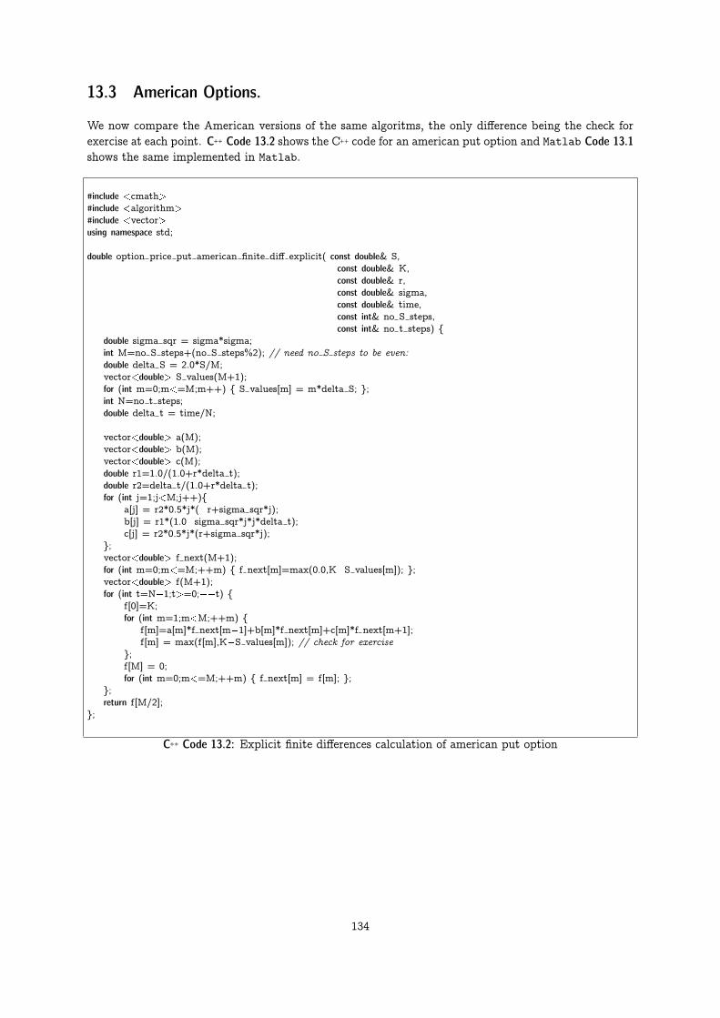
13.3 American Options.
We now compare the American versions of the same algoritms, the only difference being the check forexercise at each point. C++ Code 13.2 shows the C++ code for an american put option and Matlab Code 13.1shows the same implemented in Matlab.
#include <cmath>#include <algorithm>#include <vector>using namespace std;
double option price put american finite diff explicit( const double& S,const double& K,const double& r,const double& sigma,const double& time,const int& no S steps,const int& no t steps) {
double sigma sqr = sigma*sigma;int M=no S steps+(no S steps%2); // need no S steps to be even:double delta S = 2.0*S/M;vector<double> S values(M+1);for (int m=0;m<=M;m++) { S values[m] = m*delta S; };int N=no t steps;double delta t = time/N;
vector<double> a(M);vector<double> b(M);vector<double> c(M);double r1=1.0/(1.0+r*delta t);double r2=delta t/(1.0+r*delta t);for (int j=1;j<M;j++){
a[j] = r2*0.5*j*(�r+sigma sqr*j);b[j] = r1*(1.0�sigma sqr*j*j*delta t);c[j] = r2*0.5*j*(r+sigma sqr*j);
};vector<double> f next(M+1);for (int m=0;m<=M;++m) { f next[m]=max(0.0,K�S values[m]); };vector<double> f(M+1);for (int t=N�1;t>=0;��t) {
f[0]=K;for (int m=1;m<M;++m) {
f[m]=a[m]*f next[m�1]+b[m]*f next[m]+c[m]*f next[m+1];f[m] = max(f[m],K�S values[m]); // check for exercise
};f[M] = 0;for (int m=0;m<=M;++m) { f next[m] = f[m]; };
};return f[M/2];
};
C++ Code 13.2: Explicit finite differences calculation of american put option
134

function P = findiff exp am put(S,K,r,sigma,time,no S steps,no t steps)sigma sqr = sigma^2;M=no S steps + rem(no S steps,2); # need no S steps to be even:delta S = 2*S/M;S values = delta S * (0:M)’;N=no t steps;delta t = time/N;
r1=1/(1+r*delta t);r2=delta t/(1+r*delta t);
a=zeros(M�1,1);b=zeros(M�1,1);c=zeros(M�1,1);for j=1:M�1
a(j) = r2*0.5*j*(�r+sigma sqr*j);b(j) = r1*(1.0�sigma sqr*j*j*delta t);c(j) = r2*0.5*j*(r+sigma sqr*j);
endforf next = max(0,K�S values);for t=N�1:�1:0
f = [ K; a.*f next(1:M�1)+b.*f next(2:M)+c.*f next(3:M+1); 0];f = max(f,K�S values);f next=f;
endforP=f(1+M/2);
endfunction
Matlab Code 13.1: Explicit finite differences calculation of American put option
135

Example
Given the following parameters: S = 50, K = 50, r = 10% and � = 0:4. The time to maturity is 0.4167.
Price European and American put option prices using finite differences with 20 steps in the S dimension and11 steps in the time dimenstion.
C++ program:
double S = 50.0;double K = 50.0;double r = 0.1;double sigma = 0.4;double time=0.4167;int no S steps=20;int no t steps=11;cout << " explicit finite differences, european put price = ";cout << option price put european finite diff explicit(S,K,r,sigma,time,no S steps,no t steps)
<< endl;cout << " explicit finite differences, american put price = ";cout << option price put american finite diff explicit(S,K,r,sigma,time,no S steps,no t steps)
<< endl;
Output from C++ program:
explicit finite differences, european put price = 4.03667explicit finite differences, american put price = 4.25085
Readings Brennan and Schwartz (1978) is one of the first finance applications of finite differences.Section 14.7 of Hull (1993) has a short introduction to finite differences. Wilmott, Dewynne, and Howison(1994) is an exhaustive source on option pricing from the perspective of solving partial differentialequations.
136

13.4 Implicit finite differences
What really distinguishes C++ from standard C is the ability to extend the language by creating classesand collecting these classes into libraries. A library is a collection of classes and routines for one particularpurpose. We have already seen this idea when creating the date and term_structure classes. However,one should not necessarily always go ahead and create such classes from scratch. It is just as well to usesomebody else’s class, as long as it is correct and well documented and fulfills a particular purpose.
13.5 An example matrix class
Use Newmat as an example matrix class.
13.6 Finite Differences
We use the case of implicit finite difference calculations to illustrate matrix calculations in action.
The method of choice for any engineer given a differential equation to solve is to numerically approximateit using a finite difference scheme, which is to approximate the continous differential equation with adiscrete difference equation, and solve this difference equation.
In the following we implement implicit finite differences. Explicit finite differences was discussed earlier,we postponed the implicit case to now because it is much simplified by a matrix library.
13.7 American Options
Let us first look at how this pricing is implemented in Matlab. Matlab Code 13.2 shows the implementa-tion. Implementation of the same calculation in C++ Code 13.3 using the Newmat library and C++ Code 13.4using IT++.
function P = findiff imp am put(S,K,r,sigma,time,no S steps,no t steps)sigma sqr = sigma^2;M=no S steps + rem(no S steps,2); # need no S steps to be even:delta S = 2.0*S/double(M);S values = delta S* (1:M+1)’;N=no t steps;delta t = time/N;A = zeros(M+1,M+1);A(1,1)=1.0;for j=2:M
A(j,j�1) = 0.5*j*delta t*(r�sigma sqr*j);A(j,j) = 1.0 + delta t*(r+sigma sqr*j*j);A(j,j+1) = 0.5*j*delta t*(�r�sigma sqr*j);
endforA(M+1,M+1)=1.0;B = max(0,K�S values);F = inv(A)*B;for t=N�1:�1:1
B = F;F = inv(A)*B;F=max(F,K�S values);
endforP= F(M/2);
endfunction
Matlab Code 13.2: Calculation of price of American put using implicit finite differences
137

#include <cmath>#include "newmat.h" // definitions for newmat matrix libraryusing namespace NEWMAT;
#include <vector>#include <algorithm>using namespace std;
double option price put american finite diff implicit(const double& S,const double& K,const double& r,const double& sigma,const double& time,const int& no S steps,const int& no t steps) {
double sigma sqr = sigma*sigma;int M=no S steps + (no S steps%2); // need no S steps to be even:// int M=no S steps; if ((no S steps%2)==1) { ++M; }; // need no S steps to be even:double delta S = 2.0*S/double(M);double S values[M+1];for (int m=0;m<=M;m++) { S values[m] = m*delta S; };int N=no t steps;double delta t = time/N;
BandMatrix A(M+1,1,1); A=0.0;A.element(0,0) = 1.0;for (int j=1;j<M;++j) {
A.element(j,j�1) = 0.5*j*delta t*(r�sigma sqr*j); // a[j]A.element(j,j) = 1.0 + delta t*(r+sigma sqr*j*j); // b[j];A.element(j,j+1) = 0.5*j*delta t*(�r�sigma sqr*j); // c[j];
};A.element(M,M)=1.0;ColumnVector B(M+1);for (int m=0;m<=M;++m){ B.element(m) = max(0.0,K�S values[m]); };ColumnVector F=A.i()*B;for(int t=N�1;t>0;��t) {
B = F;F = A.i()*B;for (int m=1;m<M;++m) { // now check for exercise
F.element(m) = max(F.element(m), K�S values[m]);};
};return F.element(M/2);
};
C++ Code 13.3: Calculation of price of American put using implicit finite differences with the Newmatmatrix library
138

#include <cmath>//#include <vector>//#include <algorithm>using namespace std;
#include <itpp/base/vec.h>#include <itpp/base/mat.h>#include <itpp/base/matfunc.h>
using namespace itpp;
double option price put american finite diff implicit itpp(const double& S,const double& K,const double& r,const double& sigma,const double& time,const int& no S steps,const int& no t steps) {
double sigma sqr = sigma*sigma;int M=no S steps + (no S steps%2); // need no S steps to be even:
double delta S = 2.0*S/double(M);double S values[M+1];for (int m=0;m<=M;m++) { S values[m] = m*delta S; };int N=no t steps;double delta t = time/N;
mat A(M+1,M+1);A.zeros();A(0,0) = 1.0;for (int j=1;j<M;++j) {
A(j,j�1) = 0.5*j*delta t*(r�sigma sqr*j); // a[j]A(j,j) = 1.0 + delta t*(r+sigma sqr*j*j); // b[j];A(j,j+1) = 0.5*j*delta t*(�r�sigma sqr*j); // c[j];
};A(M,M)=1.0;vec B(M+1);for (int m=0;m<=M;++m){ B(m) = max(0.0,K�S values[m]); };mat InvA = inv(A);vec F=InvA*B;for(int t=N�1;t>0;��t) {
B = F;F = InvA*B;for (int m=1;m<M;++m) { // now check for exercise
F(m) = max(F(m), K�S values[m]);};
};return F(M/2);
};
C++ Code 13.4: Calculation of price of American put using implicit finite differences with the IT++ matrixlibrary
139

13.8 European Options
For European options we do not need to use the finite difference scheme, but for comparison purposesC++ Code 13.5 show how one would find the European price.
#include <cmath>#include "newmat.h" // definitions for newmat matrix libraryusing namespace NEWMAT;
#include <vector> // standard STL vector template#include <algorithm>using namespace std;
double option price put european finite diff implicit(const double& S,const double& K,const double& r,const double& sigma,const double& time,const int& no S steps,const int& no t steps) {
double sigma sqr = sigma*sigma;int M=no S steps + (no S steps%2); // need no S steps to be even:// int M=no S steps; if ((no S steps%2)==1) { ++M; }; // need no S steps to be even:double delta S = 2.0*S/M;vector<double> S values(M+1);for (int m=0;m<=M;m++) { S values[m] = m*delta S; };int N=no t steps;double delta t = time/N;
BandMatrix A(M+1,1,1); A=0.0;A.element(0,0) = 1.0;for (int j=1;j<M;++j) {
A.element(j,j�1) = 0.5*j*delta t*(r�sigma sqr*j); // a[j]A.element(j,j) = 1.0 + delta t*(r+sigma sqr*j*j); // b[j];A.element(j,j+1) = 0.5*j*delta t*(�r�sigma sqr*j); // c[j];
};A.element(M,M)=1.0;ColumnVector B(M+1);for (int m=0;m<=M;++m){ B.element(m) = max(0.0,K�S values[m]); };ColumnVector F=A.i()*B;for(int t=N�1;t>0;��t) {
B = F;F = A.i()*B;
};return F.element(M/2);
};
C++ Code 13.5: Calculation of price of European put using implicit finite differences
140

Exercise 13.1.
The routines above uses direct multiplication with the inverse of A. Are there alternative, numerically morestable ways of doing it?
Example
Given the parameters S = 50, K = 50, r = 0:1, � = 0:4, time=0.5, no S steps=200; no t steps=200;
1. Price European put options using both Black Scholes and implicit finite differences.
2. Price the American put option using implicit finite differences.
C++ program:
double S = 50.0; double K = 50.0;double r = 0.1; double sigma = 0.4; double time=0.5;int no S steps=200; int no t steps=200;cout << " black scholes put price = " << option price put black scholes(S,K,r,sigma,time)<< endl;cout << " implicit Euro put price = ";cout << option price put european finite diff implicit(S,K,r,sigma,time,no S steps,no t steps) << endl;cout << " implicit American put price = ";cout << option price put american finite diff implicit(S,K,r,sigma,time,no S steps,no t steps) << endl;
Output from C++ program:
black scholes put price = 4.35166implicit Euro put price = 4.34731implicit American put price = 4.60064
Matlab program:
S = 50.0;K = 50.0;r = 0.1;sigma = 0.4;time=0.5;no S steps=200;no t steps=200;P= findiff imp am put(S,K,r,sigma,time,no S steps,no t steps)
Output from Matlab program:
P = 4.6006
Exercise 13.2.
The Newmat library is only one of a large number of available matrix libraries, both public domain andcommercial offerings. Look into alternative libraries and replace Newmat with one of these alternative libraries.What needs changing in the option price formulas?
13.9 References
Hull (2011). See the natbib documentation.
141

Chapter 14
Option pricing by simulation
Contents14.1 Simulating lognormally distributed random variables . . . . . . . . . . . . . . . . . . . . . . . . 14314.2 Pricing of European Call options . . . . . . . . . . . . . . . . . . . . . . . . . . . . . . . . . 14314.3 Hedge parameters . . . . . . . . . . . . . . . . . . . . . . . . . . . . . . . . . . . . . . . . . 14414.4 More general payoffs. Function prototypes . . . . . . . . . . . . . . . . . . . . . . . . . . . . 14614.5 Improving the efficiency in simulation . . . . . . . . . . . . . . . . . . . . . . . . . . . . . . . 147
14.5.1 Control variates. . . . . . . . . . . . . . . . . . . . . . . . . . . . . . . . . . . . 14714.5.2 Antithetic variates. . . . . . . . . . . . . . . . . . . . . . . . . . . . . . . . . . . 148
14.6 More exotic options . . . . . . . . . . . . . . . . . . . . . . . . . . . . . . . . . . . . . . . . 15114.7 References . . . . . . . . . . . . . . . . . . . . . . . . . . . . . . . . . . . . . . . . . . . . 152
We now consider using Monte Carlo methods to estimate the price of an European option, and let usfirst consider the case of the “usual” European Call, which can priced by the Black Scholes equation.Since there is already a closed form solution for this case, it is not really necessary to use simulations,but we use the case of the standard call for illustrative purposes.
At maturity, a call option is worth
cT = max(0; ST �X)
At an earlier date t, the option value will be the expected present value of this.
ct = E[PV (max(0; ST �X)]
Now, an important simplifying feature of option pricing is the “risk neutral result,” which implies thatwe can treat the (suitably transformed) problem as the decision of a risk neutral decision maker, if wealso modify the expected return of the underlying asset such that this earns the risk free rate.
ct = e�r(T�t)E�[max(0; ST �X)];
where E�[�] is a transformation of the original expectation. One way to estimate the value of the call isto simulate a large number of sample values of ST according to the assumed price process, and find theestimated call price as the average of the simulated values. By appealing to a law of large numbers, thisaverage will converge to the actual call value, where the rate of convergence will depend on how manysimulations we perform.
142

14.1 Simulating lognormally distributed random variables
Lognormal variables are simulated as follows. Let ~x be normally distributed with mean zero and varianceone. If St follows a lognormal distribution, then the one-period-later price St+1 is simulated as
St+1 = Ste(r� 1
2�2)+�~x;
or more generally, if the current time is t and terminal date is T , with a time between t and T of (T � t),
ST = Ste(r� 1
2�2)(T�t)+�
pT�t~x
Simulation of lognormal random variables is illustrated by C++ Code 14.1.
#include <cmath>using namespace std;#include "normdist.h"
double simulate lognormal random variable(const double& S, // current value of variableconst double& r, // interest rateconst double& sigma, // volatitilyconst double& time) { // time to final date
double R = (r � 0.5 * pow(sigma,2) )*time;double SD = sigma * sqrt(time);return S * exp(R + SD * random normal());
};
C++ Code 14.1: Simulating a lognormally distributed random variable
14.2 Pricing of European Call options
For the purposes of doing the Monte Carlo estimation of the price of an European call
ct = e�r(T�t)E[max(0; ST �X)];
note that here one merely need to simulate the terminal price of the underlying, ST , the price of theunderlying at any time between t and T is not relevant for pricing. We proceed by simulating lognormallydistributed random variables, which gives us a set of observations of the terminal price ST . If we letST;1; ST;2; ST;3; : : : ST;n denote the n simulated values, we will estimate E�[max(0; ST�X)] as the averageof option payoffs at maturity, discounted at the risk free rate.
ct = e�r(T�t)
nXi=1
max (0; ST;i �X)
!
C++ Code 14.2 shows the implementation of a Monte Carlo estimation of an European call option.
Example
Given S = 100, K = 100, r = 0:1, � = 0:25, time=1. Use 5000 simulations. Price put and call option usingBlack Scholes and simulation.
143
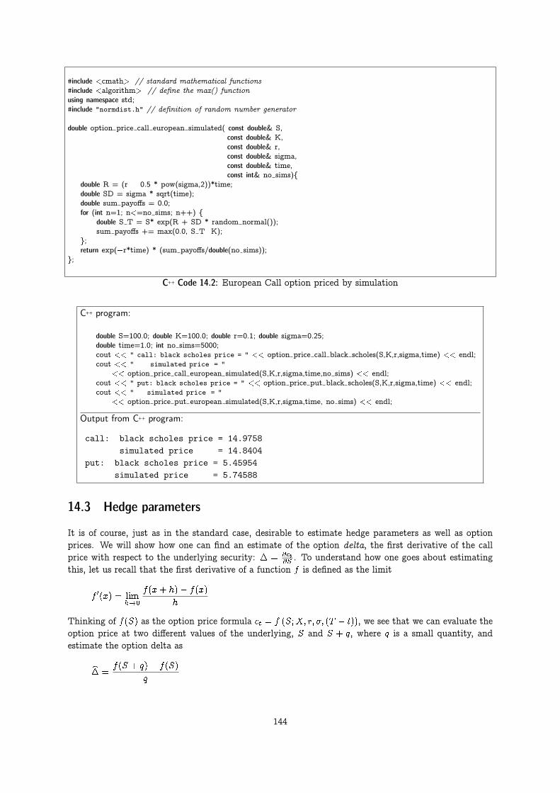
#include <cmath> // standard mathematical functions#include <algorithm> // define the max() functionusing namespace std;#include "normdist.h" // definition of random number generator
double option price call european simulated( const double& S,const double& K,const double& r,const double& sigma,const double& time,const int& no sims){
double R = (r � 0.5 * pow(sigma,2))*time;double SD = sigma * sqrt(time);double sum payoffs = 0.0;for (int n=1; n<=no sims; n++) {
double S T = S* exp(R + SD * random normal());sum payoffs += max(0.0, S T�K);
};return exp(�r*time) * (sum payoffs/double(no sims));
};
C++ Code 14.2: European Call option priced by simulation
C++ program:
double S=100.0; double K=100.0; double r=0.1; double sigma=0.25;double time=1.0; int no sims=5000;cout << " call: black scholes price = " << option price call black scholes(S,K,r,sigma,time) << endl;cout << " simulated price = "
<< option price call european simulated(S,K,r,sigma,time,no sims) << endl;cout << " put: black scholes price = " << option price put black scholes(S,K,r,sigma,time) << endl;cout << " simulated price = "
<< option price put european simulated(S,K,r,sigma,time, no sims) << endl;
Output from C++ program:
call: black scholes price = 14.9758simulated price = 14.8404
put: black scholes price = 5.45954simulated price = 5.74588
14.3 Hedge parameters
It is of course, just as in the standard case, desirable to estimate hedge parameters as well as optionprices. We will show how one can find an estimate of the option delta, the first derivative of the callprice with respect to the underlying security: � = @ct
@S . To understand how one goes about estimatingthis, let us recall that the first derivative of a function f is defined as the limit
f 0(x) = limh!0
f(x+ h)� f(x)
h
Thinking of f(S) as the option price formula ct = f (S;X; r; �; (T � t)), we see that we can evaluate theoption price at two different values of the underlying, S and S + q, where q is a small quantity, andestimate the option delta as
b� =f(S + q)� f(S)
q
144

In the case of Monte Carlo estimation, it is very important that this is done by using the same sequenceof random variables to estimate the two option prices with prices of the underlying S and S + q.C++ Code 14.3 implements this estimation of the option delta.
#include <cmath> // standard mathematical functions#include <algorithm> // define the max() functionusing namespace std;#include "normdist.h" // definition of random number generator
double option price delta call european simulated(const double& S,const double& K,const double& r,const double& sigma,const double& time,const int& no sims){
double R = (r � 0.5 * pow(sigma,2))*time;double SD = sigma * sqrt(time);double sum payoffs = 0.0;double sum payoffs q = 0.0;double q = S*0.01;for (int n=1; n<=no sims; n++) {
double Z = random normal();double S T = S* exp(R + SD * Z);sum payoffs += max(0.0, S T�K);double S T q = (S+q)* exp(R + SD * Z);sum payoffs q += max(0.0, S T q�K);
};double c = exp(�r*time) * (sum payoffs/no sims);double c q = exp(�r*time) * (sum payoffs q/no sims);return (c q�c)/q;
};
C++ Code 14.3: Estimate Delta of European Call option priced by Monte Carlo
One can estimate other hedge parameters in a simular way.
Example
Given S = 100, K = 100, r = 0:1, � = 0:25, time=1. Use 5000 simulations. Calculate deltas of put and calloption using Black Scholes and simulation.
C++ program:
double S=100.0; double K=100.0; double r=0.1; double sigma=0.25;double time=1.0; int no sims=5000;cout << " call: bs delta = " << option price delta call black scholes(S,K,r,sigma,time)
<< " sim delta = " << option price delta call european simulated(S,K,r,sigma,time,no sims)<< endl;
cout << " put: bs delta = " << option price delta put black scholes(S,K,r,sigma,time)<< " sim delta = " << option price delta put european simulated(S,K,r,sigma,time,no sims)<< endl;
Output from C++ program:
call: bs delta = 0.700208 sim delta = 0.701484put: bs delta = -0.299792 sim delta = -0.307211
145
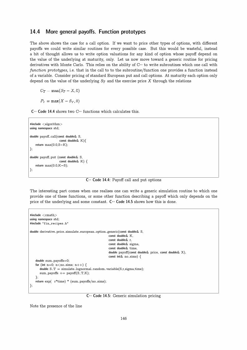
14.4 More general payoffs. Function prototypes
The above shows the case for a call option. If we want to price other types of options, with differentpayoffs we could write similar routines for every possible case. But this would be wasteful, insteada bit of thought allows us to write option valuations for any kind of option whose payoff depend onthe value of the underlying at maturity, only. Let us now move toward a generic routine for pricingderivatives with Monte Carlo. This relies on the ability of C++ to write subroutines which one call withfunction prototypes, i.e. that in the call to to the subroutine/function one provides a function insteadof a variable. Consider pricing of standard European put and call options. At maturity each option onlydepend on the value of the underlying ST and the exercise price X through the relations
CT = max(ST �X; 0)
PT = max(X � ST ; 0)
C++ Code 14.4 shows two C++ functions which calculates this.
#include <algorithm>using namespace std;
double payoff call(const double& S,const double& K){
return max(0.0,S�K);};
double payoff put (const double& S,const double& K) {
return max(0.0,K�S);};
C++ Code 14.4: Payoff call and put options
The interesting part comes when one realises one can write a generic simulation routine to which oneprovide one of these functions, or some other function describing a payoff which only depends on theprice of the underlying and some constant. C++ Code 14.5 shows how this is done.
#include <cmath>using namespace std;#include "fin_recipes.h"
double derivative price simulate european option generic(const double& S,const double& K,const double& r,const double& sigma,const double& time,double payoff(const double& price, const double& X),const int& no sims) {
double sum payoffs=0;for (int n=0; n<no sims; n++) {
double S T = simulate lognormal random variable(S,r,sigma,time);sum payoffs += payoff(S T,K);
};return exp(�r*time) * (sum payoffs/no sims);
};
C++ Code 14.5: Generic simulation pricing
Note the presence of the line
146

double payoff(const double& S, const double& K),
in the subroutine call. When this function is called, the calling program will need to provide a functionto put there, such as the Black Scholes example above. The next example shows a complete example ofhow this is done.
Example
Given S = 100, K = 100, r = 0:1, � = 0:25, time=1, no sims=5000.
C++ program:
double S = 100; double K = 100; double r = 0.1;double sigma = 0.25; double time = 1.0; int no sims = 50000;cout << "Black Scholes call option price = " << option price call black scholes(S,K,r,sigma,time) << endl;cout << "Simulated call option price = "
<< derivative price simulate european option generic(S,K,r,sigma,time,payoff call,no sims)<< endl;
cout << "Black Scholes put option price = " << option price put black scholes(S,K,r,sigma,time) << endl;cout << "Simulated put option price = "
<< derivative price simulate european option generic(S,K,r,sigma,time,payoff put,no sims)<< endl;
Output from C++ program:
Black Scholes call option price = 14.9758Simulated call option price = 14.995Black Scholes put option price = 5.45954Simulated put option price = 5.5599
As we see, even with as many as 50,000 simuations, the option prices estimated using Monte Carlo stilldiffers substantially from the “true” values.
14.5 Improving the efficiency in simulation
There are a number of ways of “improving” the implementation of Monte Carlo estimation such that theestimate is closer to the true value.
14.5.1 Control variates.
One is the method of control variates. The idea is simple. When one generates the set of terminal valuesof the underlying security, one can value several derivatives using the same set of terminal values. Whatif one of the derivatives we value using the terminal values is one which we have an analytical solutionto? For example, suppose we calculate the value of an at the money European call option using boththe (analytical) Black Scholes formula and Monte Carlo simulation. If it turns out that the Monte Carloestimate overvalues the option price, we think that this will also be the case for other derivatives valuedusing the same set of simulated terminal values. We therefore move the estimate of the price of thederivative of interest downwards.
Thus, suppose we want to value an European put and we use the price of an at the money Europeancall as the control variate. Using the same set of simulated terminal values ST;i, we estimate the twooptions using Monte Carlo as:
pt = e�r(T�t)
nXi=1
max (0; X � ST;i)
!
147
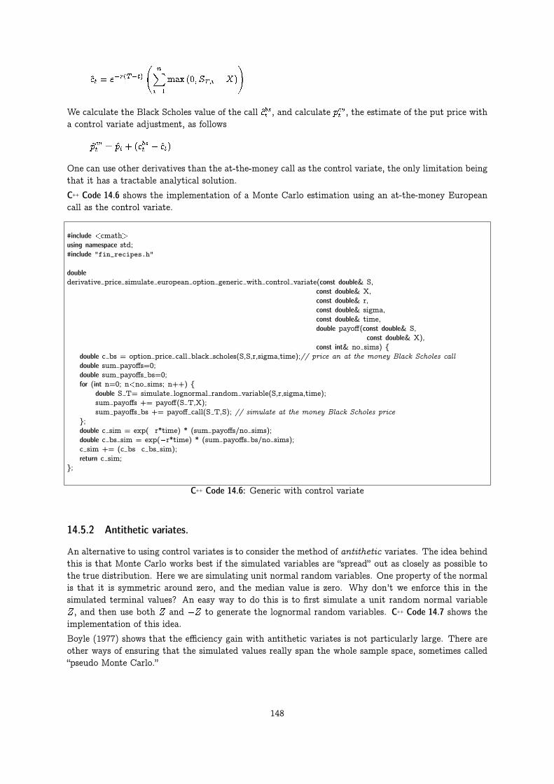
ct = e�r(T�t)
nXi=1
max (0; ST;i �X)
!
We calculate the Black Scholes value of the call cbst , and calculate pcvt , the estimate of the put price witha control variate adjustment, as follows
pcvt = pt + (cbst � ct)
One can use other derivatives than the at-the-money call as the control variate, the only limitation beingthat it has a tractable analytical solution.
C++ Code 14.6 shows the implementation of a Monte Carlo estimation using an at-the-money Europeancall as the control variate.
#include <cmath>using namespace std;#include "fin_recipes.h"
doublederivative price simulate european option generic with control variate(const double& S,
const double& X,const double& r,const double& sigma,const double& time,double payoff(const double& S,
const double& X),const int& no sims) {
double c bs = option price call black scholes(S,S,r,sigma,time);// price an at the money Black Scholes calldouble sum payoffs=0;double sum payoffs bs=0;for (int n=0; n<no sims; n++) {
double S T= simulate lognormal random variable(S,r,sigma,time);sum payoffs += payoff(S T,X);sum payoffs bs += payoff call(S T,S); // simulate at the money Black Scholes price
};double c sim = exp(�r*time) * (sum payoffs/no sims);double c bs sim = exp(�r*time) * (sum payoffs bs/no sims);c sim += (c bs�c bs sim);return c sim;
};
C++ Code 14.6: Generic with control variate
14.5.2 Antithetic variates.
An alternative to using control variates is to consider the method of antithetic variates. The idea behindthis is that Monte Carlo works best if the simulated variables are “spread” out as closely as possible tothe true distribution. Here we are simulating unit normal random variables. One property of the normalis that it is symmetric around zero, and the median value is zero. Why don’t we enforce this in thesimulated terminal values? An easy way to do this is to first simulate a unit random normal variableZ, and then use both Z and �Z to generate the lognormal random variables. C++ Code 14.7 shows theimplementation of this idea.
Boyle (1977) shows that the efficiency gain with antithetic variates is not particularly large. There areother ways of ensuring that the simulated values really span the whole sample space, sometimes called“pseudo Monte Carlo.”
148

#include "fin_recipes.h"#include "normdist.h"#include <cmath>using namespace std;
doublederivative price simulate european option generic with antithetic variate(const double& S,
const double& K,const double& r,const double& sigma,const double& time,double payoff(const double& S,
const double& X),const int& no sims) {
double R = (r � 0.5 * pow(sigma,2) )*time;double SD = sigma * sqrt(time);double sum payoffs=0;for (int n=0; n<no sims; n++) {
double x=random normal();double S1 = S * exp(R + SD * x);sum payoffs += payoff(S1,K);double S2 = S * exp(R + SD * (�x));sum payoffs += payoff(S2,K);
};return exp(�r*time) * (sum payoffs/(2*no sims));
};
C++ Code 14.7: Generic with antithetic variates
149

Example
Given S = 100, K = 100, r = 0:1, � = 0:25, time=1, no sims=50000. Price put and call option using BlackScholes and simulation. The simulation is to use both control variates and anthitetic methods.
C++ program:
double S = 100; double K = 100; double r = 0.1;double sigma = 0.25; double time = 1; int no sims = 50000;cout << "Black Scholes call option price = "
<< option price call black scholes(S,K,r,sigma,time) << endl;cout << "Simulated call option price = "
<< derivative price simulate european option generic(S,K,r,sigma,time, payoff call,no sims)<< endl;
cout << "Simulated call option price, CV = "<< derivative price simulate european option generic with control variate(S,K,r,sigma,time,
payoff call,no sims)<< endl;
cout << "Simulated call option price, AV = "<< derivative price simulate european option generic with antithetic variate(S,K,r,sigma,time,
payoff call,no sims)<< endl;
cout << "Black Scholes put option price = " << option price put black scholes(S,K,r,sigma,time) << endl;cout << "Simulated put option price = "
<< derivative price simulate european option generic(S,K,r,sigma,time,payoff put,no sims) << endl;cout << "Simulated put option price, CV = "
<< derivative price simulate european option generic with control variate(S,K,r,sigma,time,payoff put,no sims)
<< endl;cout << "Simulated put option price, AV = "
<< derivative price simulate european option generic with antithetic variate(S,K,r,sigma,time,payoff put,no sims)
<< endl;
Output from C++ program:
Black Scholes call option price = 14.9758Simulated call option price = 14.995Simulated call option price, CV = 14.9758Simulated call option price, AV = 14.9919Black Scholes put option price = 5.45954Simulated put option price = 5.41861Simulated put option price, CV = 5.42541Simulated put option price, AV = 5.46043
150
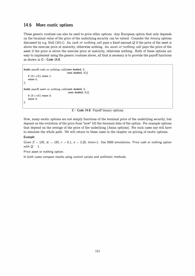
14.6 More exotic options
These generic routines can also be used to price other options. Any European option that only dependson the terminal value of the price of the underlying security can be valued. Consider the binary optionsdiscussed by e.g. Hull (2011). An cash or nothing call pays a fixed amount Q if the price of the asset isabove the exercise price at maturity, otherwise nothing. An asset or nothing call pays the price of theasset if the price is above the exercise price at maturity, otherwise nothing. Both of these options areeasy to implement using the generic routines above, all that is necesary is to provide the payoff functionsas shown in C++ Code 14.8.
double payoff cash or nothing call(const double& S,const double& K){
if (S>=K) return 1;return 0;
};
double payoff asset or nothing call(const double& S,const double& K){
if (S>=K) return S;return 0;
};
C++ Code 14.8: Payoff binary options
Now, many exotic options are not simply functions of the terminal price of the underlying security, butdepend on the evolution of the price from “now” till the terminal date of the option. For example optionsthat depend on the average of the price of the underlying (Asian options). For such cases one will haveto simulate the whole path. We will return to these cases in the chapter on pricing of exotic options.
Example
Given S = 100, K = 100, r = 0:1, � = 0:25, time=1. Use 5000 simulations. Price cash or nothing optionwith Q = 1.
Price asset or nothing option.
In both cases compare results using control variate and anthitetic methods.
151

C++ program:
double S=100.0; double K=100.0; double r=0.1; double sigma=0.25;double time=1.0; int no sims=5000;cout << " cash or nothing, Q=1: "
<< derivative price simulate european option generic(S,K,r,sigma,time,payoff cash or nothing call,no sims)
<< endl;cout << " control variate "
<< derivative price simulate european option generic with control variate(S,K,r,sigma,time,payoff cash or nothing call,no sims)
<< endl;cout << " antithetic variate "
<< derivative price simulate european option generic with antithetic variate(S,K,r,sigma,time,payoff cash or nothing call,no sims)
<< endl;cout << " asset or nothing: "
<< derivative price simulate european option generic(S,K,r,sigma,time,payoff asset or nothing call,no sims)
<< endl;cout << " control variate "
<< derivative price simulate european option generic with control variate(S,K,r,sigma,time,payoff asset or nothing call,no sims)
<< endl;cout << " antithetic variate "
<< derivative price simulate european option generic with antithetic variate(S,K,r,sigma,time,payoff asset or nothing call,no sims)
<< endl;
Output from C++ program:
cash or nothing, Q=1: 0.547427control variate 1.02552antithetic variate 0.549598asset or nothing: 70.5292control variate 69.8451antithetic variate 70.2205
Exercise 14.1.
Consider the pricing of an European Call option as implemented in code 14.2, and the generic formula forpricing with Monte Carlo for European options that only depend on the terminal value of the underlyingsecurity, as implemented in code 14.5.
Note the difference in the implementation of the lognormal simulation of terminal values. Why can one arguethat the first implementation is more efficient than the other?
14.7 References
Boyle (1977) is a good early source on the use of the Monte Carlo technique for pricing derivatives.Simulation is also covered in Hull (2011).
152

Chapter 15
Pricing American Options – Approximations
Contents15.1 The Johnson (1983) approximation . . . . . . . . . . . . . . . . . . . . . . . . . . . . . . . . 15315.2 An approximation to the American Put due to Geske and Johnson (1984) . . . . . . . . . . . . 15615.3 A quadratic approximation to American prices due to Barone–Adesi and Whaley. . . . . . . . . . 15915.4 An alternative approximation to american options due to Bjerksund and Stensland (1993) . . . . 16215.5 Readings . . . . . . . . . . . . . . . . . . . . . . . . . . . . . . . . . . . . . . . . . . . . . 165
There has been developed some useful approximations to various specific options. It is of course Amer-ican options that are approximated. We will look at a number of approximations, both for their intrinsicusefulness, but also as examples of different approaches to generating an approximated value. The firstwe will look at is the Johnson (1983) approximation to an American put. This is a purely empiricalapproach to estimating the functional forms, with parameters estimated using regressions. The Geskeand Johnson (1984) approach is to view the American option as a the limit of a sequence of Bermudanoptions with increasing number of exercise dates. The American value is found by interpolating forwardthe Bermudan values. The Barone-Adesi and Whaley (1987) approximation decomposes the Americanoption into two, the European value, and the early exercise premium. The early exercise premium isrelatively small, and is easier to approximate. Finally, the Bjerksund and Stensland (1993) is an exampleof bounding the option value by finding a lower bound on its value. A typical approach to doing so isto specify some (suboptimal) exercise strategy. As soon as the exercise strategy is known, the option iseasily valued.
Approximations are useful, but they should be used with caution. Typically, an approximation workswell within a range of parameter values, but can go seriously wrong for some unfortunate combinationof parameters. The user is well advised to to consider alternative approximations, and at a minimumuse the price of the corresponding European option as a “sanity check” in the calculations. (In fact, inseveral of the following routines values are checked against Black Scholes values.)
15.1 The Johnson (1983) approximation
An early attempt at an analytical approximation to the price of an American put is provided by Johnson(1983). Formula 15.1 provides the details, and C++ Code 15.1 provides the implementation.
Example
Using the parameters r = 0:125, S = 1:1, X = 1, � = 0:5 and time to maturity of one year, calculate theprice of an american call using the Johnson (1983) approximation.
153

P (X) = �p�Xer(T�t)
�+ (1� �)p (X)
� =
�r(T � t)
a0r(T � t) + a1
�l; where l =
ln(S=Sc)
ln(X=Sc)
Sc = X
�
1 +
�m; where m =
�2(T � t)
b0�2(T � t) + b1 = 2r=�2
The constants a0, a1, b1 and b2 are constants. Their parameter values are estimated as
a0 = 3:9649 a1 = 0:032325
b0 = 1:040803 b1 = 0:00963
S: Current value of underlying security. X: Exercise price of american put. �: Volatility of underlying. r: risk freee interest rate.(T � t): Time to maturity for option.
Formula 15.1: The functional form of the Johnson (1983) approximation to the value of an American put
C++ program:
double r=0.125; double S=1.1; double X=1;double sigma=0.5; double time = 1;cout << " American put price using Johnson approximation = "
<< option price american put approximated johnson(S, X, r, sigma, time)<< endl;
Output from C++ program:
American put price using Johnson approximation = 0.11582
Barone-Adesi (2005) notes that this approximation is inaccurate outside of the parameter range consid-ered in the paper.
154
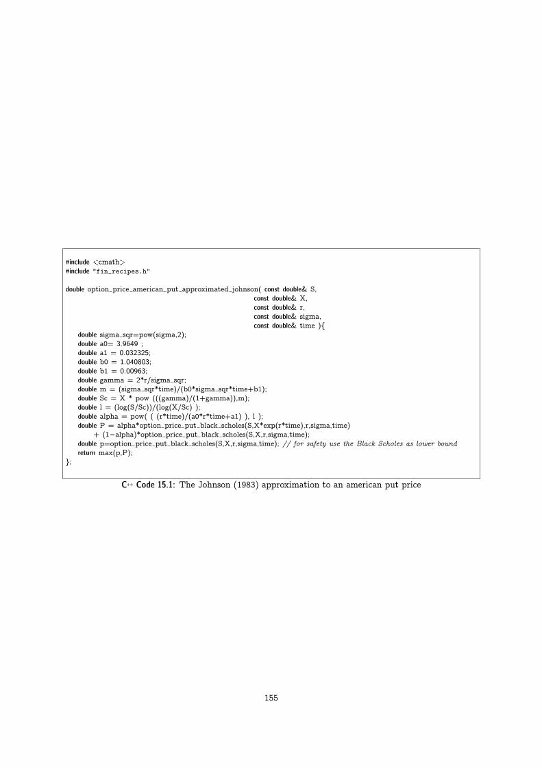
#include <cmath>#include "fin_recipes.h"
double option price american put approximated johnson( const double& S,const double& X,const double& r,const double& sigma,const double& time ){
double sigma sqr=pow(sigma,2);double a0= 3.9649 ;double a1 = 0.032325;double b0 = 1.040803;double b1 = 0.00963;double gamma = 2*r/sigma sqr;double m = (sigma sqr*time)/(b0*sigma sqr*time+b1);double Sc = X * pow (((gamma)/(1+gamma)),m);double l = (log(S/Sc))/(log(X/Sc) );double alpha = pow( ( (r*time)/(a0*r*time+a1) ), l );double P = alpha*option price put black scholes(S,X*exp(r*time),r,sigma,time)
+ (1�alpha)*option price put black scholes(S,X,r,sigma,time);double p=option price put black scholes(S,X,r,sigma,time); // for safety use the Black Scholes as lower boundreturn max(p,P);
};
C++ Code 15.1: The Johnson (1983) approximation to an american put price
155
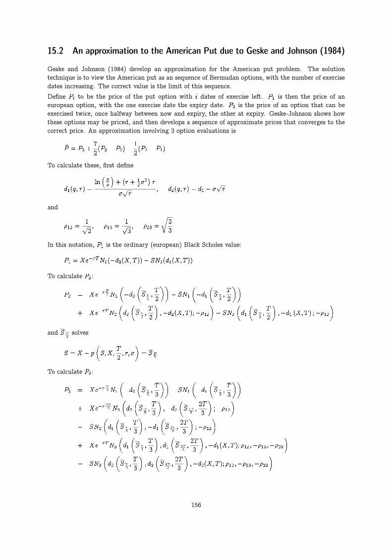
15.2 An approximation to the American Put due to Geske and Johnson (1984)
Geske and Johnson (1984) develop an approximation for the American put problem. The solutiontechnique is to view the American put as an sequence of Bermudan options, with the number of exercisedates increasing. The correct value is the limit of this sequence.
Define Pi to be the price of the put option with i dates of exercise left. P1 is then the price of aneuropean option, with the one exercise date the expiry date. P2 is the price of an option that can beexercised twice, once halfway between now and expiry, the other at expiry. Geske-Johnson shows howthese options may be priced, and then develops a sequence of approximate prices that converges to thecorrect price. An approximation involving 3 option evaluations is
P = P3 +7
2(P3 � P2)� 1
2(P2 � P1)
To calculate these, first define
d1(q; � ) =ln�Sq
�+�r + 1
2�2��
�p�
; d2(q; � ) = d1 � �p�
and
�12 =1p2; �13 =
1p3; �23 =
r2
3
In this notation, P1 is the ordinary (european) Black Scholes value:
P1 = Xe�rTN1(�d2(X;T ))� SN1(d1(X;T ))
To calculate P2:
P2 = Xe�rT2 N1
��d2
�S T
2;T
2
��� SN1
��d1
�S T
2;T
2
��+ Xe�rTN2
�d2
�S T
2;T
2
�;�d2(X;T );��12
�� SN2
�d1
�S T
2;T
2
�;�d1 (X;T ) ;��12
�and S T
2solves
S = X � p
�S;X;
T
2; r; �
�= S T
2
To calculate P3:
P3 = Xe�rT3 N1
��d2
�S T
3;T
3
��� SN1
��d1
�S T
3;T
3
��+ Xe�r
2T3 N2
�d2
�S T
3;T
3
�;�d2
�S 2T
3;2T
3
�;��12
�� SN2
�d1
�S T
3;T
3
�;�d1
�S 2T
3;2T
3
�;��12
�+ Xe�rTN3
�d1
�S T
3;T
3
�; d1
�S 2T
3;2T
3
�;�d1(X;T ); �12;��13;��23
�� SN3
�d2
�S T
3;T
3
�; d2
�S 2T
3;2T
3
�;�d2(X;T ); �12;��13;��23
�
156

where the critical stock prices solves
S = X � P2
�S;X;
2T
3; r; �
�= ST=3
S = X � p
�S;X;
T
3; r; �
�= S2T=3
The main issue in implementation of this formula (besides keeping the notation straight) is the evaluta-tion of P3, since it involves the evaluation of a trivariate normal cumulative distribution. The evaluationof N3() is described later, since it involves calls to external routines for numerical intergration.
To solve for
S = X � p
�S;X;
T
2; r; �
�= S T
2
involves Newton steps. Define
g(S) = S �X + p
�S;X;
T
2; r; �
�Iterate on S
Si = Si � g
g0
until g is equal to zero with some given tolerance.
157

#include <cmath>#include "normdist.h"#include "fin_recipes.h"#include <iostream>
const double ACCURACY=1e�6;
inline double d1(const double& S,const double& X, const double& r, const double& sigma, const double& tau){return (log(S/X) + (r+0.5*pow(sigma,2))*tau)/(sigma*sqrt(tau));
};
inline double d2(const double& S, const double& X, const double& r, const double& sigma, const double& tau){return d1(S,X,r,sigma,tau)�sigma*sqrt(tau);
};
inline double calcP2(const double& S, const double& X, const double& r, const double& sigma, const double& time,const double& t2, const double& S2 bar, const double& rho12){
double P2 = X*exp(�r*t2)*N(�d2(S,S2 bar,r,sigma,t2));P2 �= S*N(�d1(S,S2 bar,r,sigma,t2));P2 += X*exp(�r*time)*N(d2(S,S2 bar,r,sigma,t2),�d2(S,X,r,sigma,time),�rho12);P2 �= S*N(d1(S,S2 bar,r,sigma,t2),�d1(S,X,r,sigma,time),�rho12);return P2;
};
double option price american put approximated geske johnson( const double& S, const double& X, const double& r,const double& sigma, const double& time ){
double P1 = option price put black scholes(S,X,r,sigma,time);double rho12=1.0/sqrt(2.0); double rho13=1.0/sqrt(3.0); double rho23=sqrt(2.0/3.0);double t2 = time/2.0; double t23 = time*2.0/3.0; double t3 = time/3.0;double Si=S; double S2 bar=S;double g=1; double gprime=1;while (fabs(g)>ACCURACY){
g=Si�X+option price put black scholes(Si,X,r,sigma,t2);gprime=1.0+option price delta put black scholes(Si,X,r,sigma,t2);S2 bar=Si;Si=Si�g/gprime;
};double P2 = calcP2(S,X,r,sigma,time,t2,S2 bar,rho12);P2=max(P1,P2); // for safety, use one less step as lower bounddouble S23 bar=S2 bar;g=1;while (fabs(g)>ACCURACY){
g=Si�X+option price put black scholes(Si,X,r,sigma,t23);gprime=1.0+option price delta put black scholes(Si,X,r,sigma,t23);S23 bar=Si;Si=Si�g/gprime;
};double S3 bar=S23 bar;g=1;while (fabs(g)>ACCURACY){
g=Si�X+option price put black scholes(Si,X,r,sigma,t3);gprime=1.0+option price delta put black scholes(Si,X,r,sigma,t3);S3 bar=Si;Si=Si�g/gprime;
};double P3 = X * exp(�r*t3) * N(�d2(S,S3 bar,r,sigma,t3));P3 �= S * N(�d1(S,S3 bar,r,sigma,t3));P3 += X*exp(�r*time)*N(d2(S,S3 bar,r,sigma,t3),�d2(S,S23 bar,r,sigma,t23),�rho12);P3 �= S*N(d1(S,S3 bar,r,sigma,t3),�d1(S,S23 bar,r,sigma,t23),�rho12);P3 += X*exp(�r*t23)*N3(d1(S,S3 bar,r,sigma,t3),d1(S,S23 bar,r,sigma,t23),�d1(S,X,r,sigma,time),rho12,�rho13,�rho23);P3 �= S*N3(d2(S,S3 bar,r,sigma,t3),d2(S,S23 bar,r,sigma,t23),�d2(S,X,r,sigma,time),rho12,�rho13,�rho23);P3=max(P2,P3); // for safety, use one less step as lower boundreturn P3+3.5*(P3�P2)�0.5*(P2�P1);
};
C++ Code 15.2: Geske Johnson approximation of American put
158
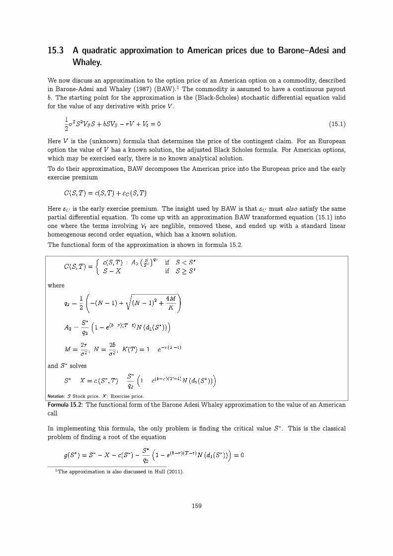
15.3 A quadratic approximation to American prices due to Barone–Adesi andWhaley.
We now discuss an approximation to the option price of an American option on a commodity, describedin Barone-Adesi and Whaley (1987) (BAW).1 The commodity is assumed to have a continuous payoutb. The starting point for the approximation is the (Black-Scholes) stochastic differential equation validfor the value of any derivative with price V .
1
2�2S2VSS + bSVS � rV + Vt = 0 (15.1)
Here V is the (unknown) formula that determines the price of the contingent claim. For an Europeanoption the value of V has a known solution, the adjusted Black Scholes formula. For American options,which may be exercised early, there is no known analytical solution.
To do their approximation, BAW decomposes the American price into the European price and the earlyexercise premium
C(S; T ) = c(S; T ) + "C(S; T )
Here "C is the early exercise premium. The insight used by BAW is that "C must also satisfy the samepartial differential equation. To come up with an approximation BAW transformed equation (15.1) intoone where the terms involving Vt are neglible, removed these, and ended up with a standard linearhomeogenous second order equation, which has a known solution.
The functional form of the approximation is shown in formula 15.2.
C(S; T ) =
�c(S; T ) + A2
�SS�
�q2 if S < S�
S �X if S � S�
where
q2 =1
2
�(N � 1) +
r(N � 1)
2+
4M
K
!
A2 =S�
q2
�1� e(b�r)(T�t)N (d1(S
�))�
M =2r
�2; N =
2b
�2; K(T ) = 1� e�r(T�t)
and S� solves
S� �X = c (S�; T ) +S�
q2
�1� e(b�r)(T�t)N (d1(S
�))�
Notation: S Stock price. X: Exercise price.
Formula 15.2: The functional form of the Barone Adesi Whaley approximation to the value of an Americancall
In implementing this formula, the only problem is finding the critical value S�. This is the classicalproblem of finding a root of the equation
g(S�) = S� �X � c(S�)� S�
q2
�1� e(b�r)(T�t)N (d1(S
�))�= 0
1The approximation is also discussed in Hull (2011).
159
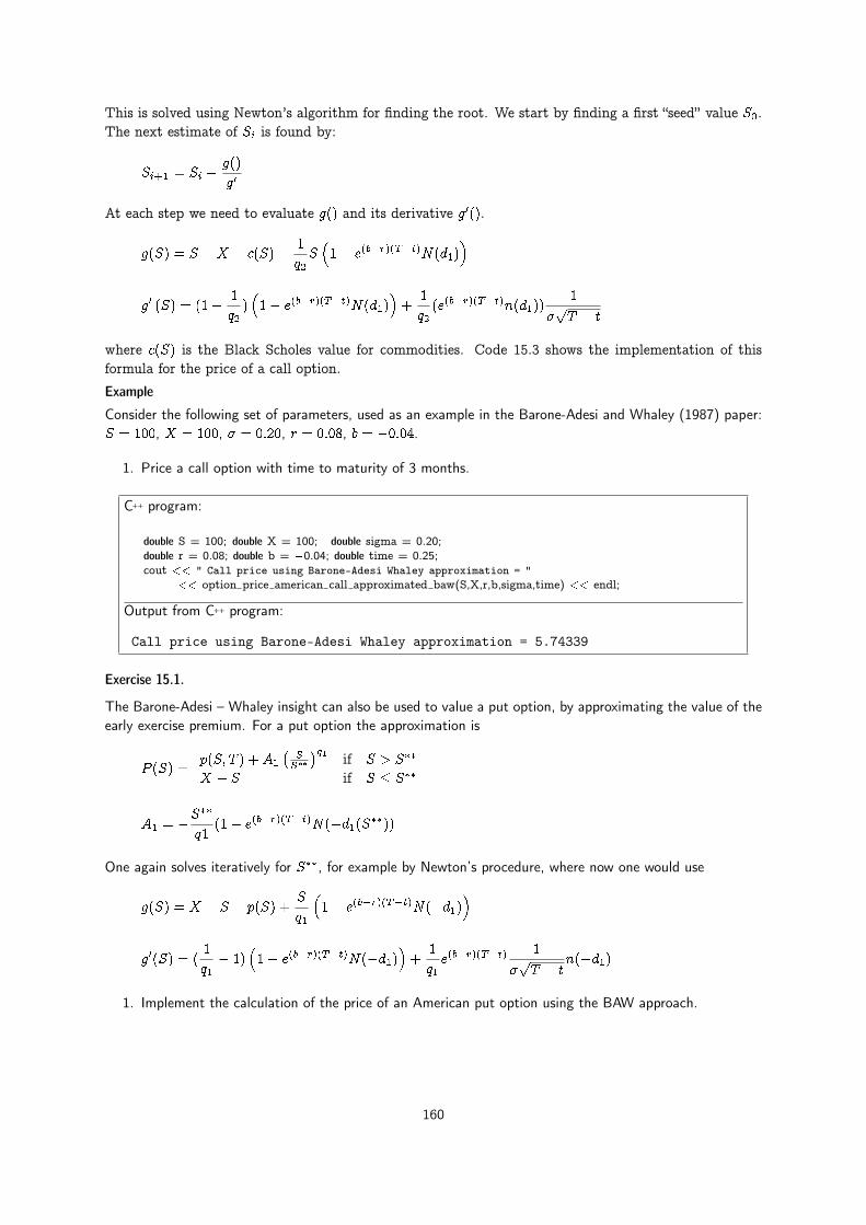
This is solved using Newton’s algorithm for finding the root. We start by finding a first “seed” value S0.The next estimate of Si is found by:
Si+1 = Si � g()
g0
At each step we need to evaluate g() and its derivative g0().
g(S) = S �X � c(S)� 1
q2S�1� e(b�r)(T�t)N(d1)
�
g0 (S) = (1� 1
q2)�1� e(b�r)(T�t)N(d1)
�+
1
q2(e(b�r)(T�t)n(d1))
1
�pT � t
where c(S) is the Black Scholes value for commodities. Code 15.3 shows the implementation of thisformula for the price of a call option.
Example
Consider the following set of parameters, used as an example in the Barone-Adesi and Whaley (1987) paper:S = 100, X = 100, � = 0:20, r = 0:08, b = �0:04.
1. Price a call option with time to maturity of 3 months.
C++ program:
double S = 100; double X = 100; double sigma = 0.20;double r = 0.08; double b = �0.04; double time = 0.25;cout << " Call price using Barone-Adesi Whaley approximation = "
<< option price american call approximated baw(S,X,r,b,sigma,time) << endl;
Output from C++ program:
Call price using Barone-Adesi Whaley approximation = 5.74339
Exercise 15.1.
The Barone-Adesi – Whaley insight can also be used to value a put option, by approximating the value of theearly exercise premium. For a put option the approximation is
P (S) =p(S; T ) + A1
�SS��
�q1 if S > S��
X � S if S � S��
A1 = �S��
q1(1� e(b�r)(T�t)N(�d1(S��))
One again solves iteratively for S��, for example by Newton’s procedure, where now one would use
g(S) = X � S � p(S) +S
q1
�1� e(b�r)(T�t)N(�d1)
�
g0(S) = (1
q1� 1)
�1� e(b�r)(T�t)N(�d1)
�+
1
q1e(b�r)(T�t)
1
�pT � t
n(�d1)
1. Implement the calculation of the price of an American put option using the BAW approach.
160

#include <cmath>#include <algorithm>using namespace std;#include "normdist.h" // normal distribution#include "fin_recipes.h" // define other option pricing formulas
const double ACCURACY=1.0e�6;
double option price american call approximated baw( const double& S,const double& X,const double& r,const double& b,const double& sigma,const double& time) {
double sigma sqr = sigma*sigma;double time sqrt = sqrt(time);double nn = 2.0*b/sigma sqr;double m = 2.0*r/sigma sqr;double K = 1.0�exp(�r*time);double q2 = (�(nn�1)+sqrt(pow((nn�1),2.0)+(4*m/K)))*0.5;
double q2 inf = 0.5 * ( �(nn�1) + sqrt(pow((nn�1),2.0)+4.0*m)); // seed value from paperdouble S star inf = X / (1.0 � 1.0/q2 inf);double h2 = �(b*time+2.0*sigma*time sqrt)*(X/(S star inf�X));double S seed = X + (S star inf�X)*(1.0�exp(h2));
int no iterations=0; // iterate on S to find S star, using Newton stepsdouble Si=S seed;double g=1;double gprime=1.0;while ((fabs(g) > ACCURACY)
&& (fabs(gprime)>ACCURACY) // to avoid exploding Newton’s&& ( no iterations++<500)&& (Si>0.0)) {
double c = option price european call payout(Si,X,r,b,sigma,time);double d1 = (log(Si/X)+(b+0.5*sigma sqr)*time)/(sigma*time sqrt);g=(1.0�1.0/q2)*Si�X�c+(1.0/q2)*Si*exp((b�r)*time)*N(d1);gprime=( 1.0�1.0/q2)*(1.0�exp((b�r)*time)*N(d1))
+(1.0/q2)*exp((b�r)*time)*n(d1)*(1.0/(sigma*time sqrt));Si=Si�(g/gprime);
};double S star = 0;if (fabs(g)>ACCURACY) { S star = S seed; } // did not convergeelse { S star = Si; };double C=0;double c = option price european call payout(S,X,r,b,sigma,time);if (S>=S star) {
C=S�X;}else {
double d1 = (log(S star/X)+(b+0.5*sigma sqr)*time)/(sigma*time sqrt);double A2 = (1.0�exp((b�r)*time)*N(d1))* (S star/q2);C=c+A2*pow((S/S star),q2);
};return max(C,c); // know value will never be less than BS value
};
C++ Code 15.3: Barone Adesi quadratic approximation to the price of a call option
161

15.4 An alternative approximation to american options due to Bjerksund andStensland (1993)
Bjerksund and Stensland (1993) provides an alternative approximation to the price of American options.Their approximation is an example of calculating a lower bound for the option value. Their valua-tion relies on using an exercise strategy that is known, and although suboptimal, close enough to the(unknown) exercise strategy that the approximated value is
The corresponding put option can be estimated as
P (S;X; T; r; b; �) = C(X;S; T; r � b;�b; �)
162
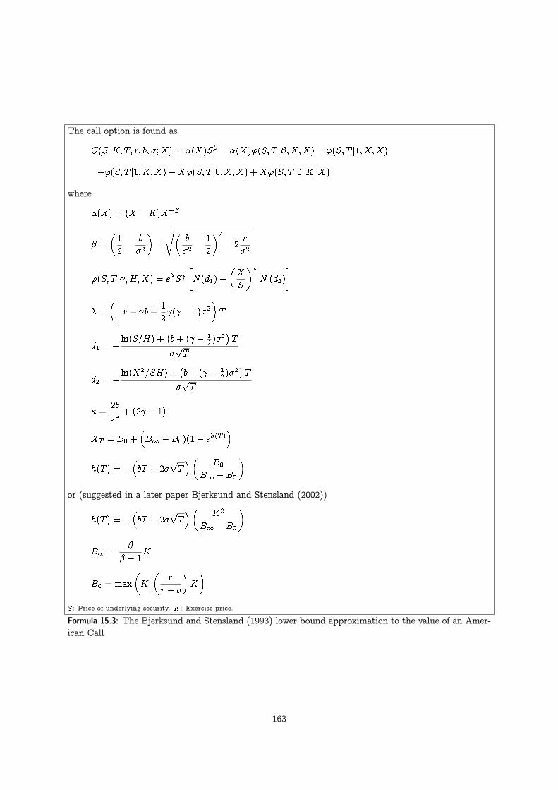
The call option is found as
C(S;K; T; r; b; �;X) = �(X)S� � �(X)'(S; T j�;X;X) + '(S; T j1; X;X)
�'(S; T j1;K;X)�X'(S; T j0; X;X) +X'(S; T j0;K;X)
where
�(X) = (X �K)X��
� =
�1
2� b
�2
�+
s�b
�2� 1
2
�2
+ 2r
�2
'(S; T j ;H;X) = e�S �N(d1)�
�X
S
��N (d2)
�
� =
��r + b+
1
2 ( � 1)�2
�T
d1 = � ln(S=H) +�b+ ( � 1
2 )�2�T
�pT
d2 = � ln(X2=SH) +�b+ ( � 1
2 )�2�T
�pT
� =2b
�2+ (2 � 1)
XT = B0 +�B1 �B0)(1� eh(T )
�h(T ) = �
�bT + 2�
pT�� B0
B1 �B0
�or (suggested in a later paper Bjerksund and Stensland (2002))
h(T ) = ��bT + 2�
pT�� K2
B1 �B0
�
B1 =�
� � 1K
B0 = max
�K;
�r
r � b
�K
�S: Price of underlying security. K: Exercise price.
Formula 15.3: The Bjerksund and Stensland (1993) lower bound approximation to the value of an Amer-ican Call
163

#include "fin_recipes.h"#include <cmath>#include "normdist.h"
inline double phi(double S, double T, double gamma, double H, double X, double r, double b, double sigma){double sigma sqr=pow(sigma,2);double kappa = 2.0*b/sigma sqr + 2.0*gamma � 1.0;double lambda = (�r + gamma * b + 0.5*gamma*(gamma�1.0)*sigma sqr)*T; // check this, says lambda in textdouble d1= � (log(S/H)+(b+(gamma�0.5)*sigma sqr)*T)/(sigma*sqrt(T));double d2= � (log((X*X)/(S*H))+(b+(gamma�0.5)*sigma sqr)*T)/(sigma*sqrt(T));double phi = exp(lambda) * pow(S,gamma) * (N(d1) � pow((X/S),kappa) * N(d2));return phi;
};
double option price american call approximated bjerksund stensland( const double& S,const double& K,const double& r,const double& b,const double& sigma,const double& T ){
double sigma sqr=pow(sigma,2);double B0=max(K,(r/(r�b)*K));double beta = (0.5 � b/sigma sqr) + sqrt( pow((b/sigma sqr�0.5),2) + 2.0 * r/sigma sqr);double Binf = beta/(beta�1.0)*K;double hT= � (b*T + 2.0*sigma*sqrt(T))*((K*K)/(Binf�B0));double XT = B0+(Binf�B0)*(1.0�exp(hT));double alpha = (XT�K)*pow(XT,�beta);double C=alpha*pow(S,beta);C �= alpha*phi(S,T,beta,XT,XT,r,b,sigma);C += phi(S,T,1,XT,XT,r,b,sigma);C �= phi(S,T,1,K,XT,r,b,sigma) ;C �= K*phi(S,T,0,XT,XT,r,b,sigma);C += K*phi(S,T,0,K,XT,r,b,sigma);double c=option price european call payout(S,K,r,b,sigma,T); // for safety use the Black Scholes as lower boundreturn max(c,C);
};
C++ Code 15.4: Approximation of American Call due to Bjerksund and Stensland (1993)
#include "fin_recipes.h"
double option price american put approximated bjerksund stensland( const double& S,const double& X,const double& r,const double& q,const double& sigma,const double& T ){
return option price american call approximated bjerksund stensland(X,S,r�(r�q),r�q,sigma,T);};
C++ Code 15.5: Approximation of American put due to Bjerksund and Stensland (1993)
164
Exercise 15.2.
An option is “At the Money Forward” if the forward price F equals the exercise price.
1. Show that a reasonable approximation to the Black Scholes value of a call option on a non-dividendpaying asset that is “At the Money Forward” is
C = 0:4�pT � tPV (F )
where F is the forward price, PV (�) signifies the present value operator, T � t is the time to maturityand � is the volatility.
15.5 Readings
See Broadie and Detemple (1996) for some comparisions of various approximations. A survey of thepricing of options, including American options, is Broadie and Detemple (2004). Barone-Adesi (2005)summarizes the history of approximating the American put.
165

Chapter 16
Average, lookback and other exotic options
Contents16.1 Bermudan options . . . . . . . . . . . . . . . . . . . . . . . . . . . . . . . . . . . . . . . . . 16616.2 Asian options . . . . . . . . . . . . . . . . . . . . . . . . . . . . . . . . . . . . . . . . . . . 16916.3 Lookback options . . . . . . . . . . . . . . . . . . . . . . . . . . . . . . . . . . . . . . . . . 17016.4 Monte Carlo Pricing of options whose payoff depend on the whole price path . . . . . . . . . . . 172
16.4.1 Generating a series of lognormally distributed variables . . . . . . . . . . . . . 17216.5 Control variate . . . . . . . . . . . . . . . . . . . . . . . . . . . . . . . . . . . . . . . . . . 17516.6 References . . . . . . . . . . . . . . . . . . . . . . . . . . . . . . . . . . . . . . . . . . . . 176
We now look at a type of options that has received a lot of attention in later years. The distinguishingfactor of these options is that they depend on the whole price path of the underlying security betweentoday and the option maturity.
16.1 Bermudan options
A Bermudan option is, as the name implies,1 a mix of an European and American option. It is astandard put or call option which can only be exercised at discrete dates throughout the life of theoption. The simplest way to do the pricing of this is again the binomial approximation, but now, insteadof checking at every node whether it is optimal to exercise early, only check at the nodes correspondingto the potential exercise times. C++ Code 16.1 shows the calculation of the Bermudan price using binomialapproximations. The times as which exercise can happen is passed as a vector argument to the routine,and in the binomial a list of which nodes exercise can happen is calculated and checked at every step.
Example
Price a Bermudan put. The following informaton is given S = 80, K = 100 r = 0.20; time = 1; � = 0:25,steps = 500, q = 0:0, Potential exercise times = 0,25, 0.5 and 0.75.
1Since Bermuda is somewhere between America and Europe...
166

C++ program:
double S=80; double K=100; double r = 0.20;double time = 1.0; double sigma = 0.25;int steps = 500;double q=0.0;vector<double> potential exercise times; potential exercise times.push back(0.25);potential exercise times.push back(0.5); potential exercise times.push back(0.75);cout << " Bermudan put price = "
<< option price put bermudan binomial(S,K,r,q,sigma,time,potential exercise times,steps)<< endl;
Output from C++ program:
Bermudan put price = 15.8869
167

#include <cmath> // standard C mathematical library#include <algorithm> // defines the max() operator#include <vector> // STL vector templatesusing namespace std;
double option price put bermudan binomial( const double& S,const double& X,const double& r,const double& q,const double& sigma,const double& time,const vector<double>& potential exercise times,const int& steps) {
double delta t=time/steps;double R = exp(r*delta t);double Rinv = 1.0/R;double u = exp(sigma*sqrt(delta t));double uu = u*u;double d = 1.0/u;double p up = (exp((r�q)*delta t)�d)/(u�d);double p down = 1.0�p up;vector<double> prices(steps+1);vector<double> put values(steps+1);
vector<int> potential exercise steps; // create list of steps at which exercise may happenfor (int i=0;i<potential exercise times.size();++i){
double t = potential exercise times[i];if ( (t>0.0)&&(t<time) ) {
potential exercise steps.push back(int(t/delta t));};
};
prices[0] = S*pow(d, steps); // fill in the endnodes.for (int i=1; i<=steps; ++i) prices[i] = uu*prices[i�1];for (int i=0; i<=steps; ++i) put values[i] = max(0.0, (X�prices[i])); // put payoffs at maturityfor (int step=steps�1; step>=0; ��step) {
bool check exercise this step=false;for (int j=0;j<potential exercise steps.size();++j){
if (step==potential exercise steps[j]) { check exercise this step=true; };};for (int i=0; i<=step; ++i) {
put values[i] = (p up*put values[i+1]+p down*put values[i])*Rinv;prices[i] = d*prices[i+1];if (check exercise this step) put values[i] = max(put values[i],X�prices[i]);
};};return put values[0];
};
C++ Code 16.1: Binomial approximation to Bermudan put option
168

16.2 Asian options
The payoff depends on the average of the underlying price. An average price call has payoff
CT = max(0; �S �X);
where �S is the average of the underlying in the period between t and T .
Another Asian is the average strike call
CT = max(0; ST � �S)
There are different types of Asians depending on how the average �S is calculated. For the case of S beinglognormal and the average �S being a geometric average, there is an analytic formula due to Kemna andVorst (1990). Hull (2011) also discusses this case. It turns out that one can calculate this option usingthe regular Black Scholes formula adjusting the volatility to �=
p3 and the dividend yield to
1
2
�r + q +
1
6�2�
in the case of continous sampling of the underlying price distribution.
C++ Code 16.2 shows the calculation of the analytical price of an Asian geometric average price call.
#include <cmath>using namespace std;#include "normdist.h" // normal distribution definitions
doubleoption price asian geometric average price call(const double& S,
const double& K,const double& r,const double& q,const double& sigma,const double& time){
double sigma sqr = pow(sigma,2);double adj div yield=0.5*(r+q+sigma sqr/6.0);double adj sigma=sigma/sqrt(3.0);double adj sigma sqr = pow(adj sigma,2);double time sqrt = sqrt(time);double d1 = (log(S/K) + (r�adj div yield + 0.5*adj sigma sqr)*time)/(adj sigma*time sqrt);double d2 = d1�(adj sigma*time sqrt);double call price = S * exp(�adj div yield*time)* N(d1) � K * exp(�r*time) * N(d2);return call price;
};
C++ Code 16.2: Analytical price of an Asian geometric average price call
Example
Relevant parameters: S = 100, K = 100, q = 0, r = 0:06, � = 0:25 and time to maturity is one year. Pricean Asian geometric average price call.
C++ program:
double S=100; double K=100; double q=0;double r=0.06; double sigma=0.25; double time=1.0;cout << " Analytical geometric average = "
<< option price asian geometric average price call(S,K,r,q,sigma,time)<< endl;
Output from C++ program:
Analytical geometric average = 6.74876
169

16.3 Lookback options
The payoff from lookback options depend on the maximum or minimum of the underlying achievedthrough the period. The payoff from the lookback call is the terminal price of the undelying less theminimum value
CT = max(0; ST � min�2[t;T ]
S� )
For this particular option an analytical solution has been found, due to Goldman, Sosin, and Gatto(1979), which is shown in Formula 16.1 and implemented in C++ Code 16.3.
C = Se�q(T�t)N(a1)� Se�q(T�t)�2
2(r � q)N(�a1)� Smine
�r(T�t)�N(a2)� �2
2(r � q)eY1N(�a3)
�
a1 =ln�
SSmin
�+ (r � q + 1
2�2)(T � t)
�pT � t
a2 = a1 � �pT � t
a3 =ln�
SSmin
�+��r + q + 1
2�2�(T � t)
�pT � t
Y1 =2�r � q � 1
2�2�ln�
SSmin
��2
Formula 16.1: Analytical formula for a lookback call
#include <cmath>using namespace std;#include "normdist.h"
double option price european lookback call(const double& S,const double& Smin,const double& r,const double& q,const double& sigma,const double& time){
if (r==q) return 0;double sigma sqr=sigma*sigma;double time sqrt = sqrt(time);double a1 = (log(S/Smin) + (r�q+sigma sqr/2.0)*time)/(sigma*time sqrt);double a2 = a1�sigma*time sqrt;double a3 = (log(S/Smin) + (�r+q+sigma sqr/2.0)*time)/(sigma*time sqrt);double Y1 = 2.0 * (r�q�sigma sqr/2.0)*log(S/Smin)/sigma sqr;return S * exp(�q*time)*N(a1)� S*exp(�q*time)*(sigma sqr/(2.0*(r�q)))*N(�a1)
� Smin * exp(�r*time)*(N(a2)�(sigma sqr/(2*(r�q)))*exp(Y1)*N(�a3));};
C++ Code 16.3: Price of lookback call option
Example
Parameters S = 100, Smin = S q = 0, r = 0:06, � = 0:346, time = 1.0, Price an European lookback call.
170

C++ program:
double S=100; double Smin=S; double q = 0; double r = 0.06;double sigma = 0.346; double time = 1.0;cout << " Lookback call price = "
<< option price european lookback call(S,Smin,r,q,sigma,time) << endl;
Output from C++ program:
Lookback call price = 27.0713
171

16.4 Monte Carlo Pricing of options whose payoff depend on the whole pricepath
Monte Carlo simulation can be used to price a lot of different options. The limitation is that the optionsshould be European. American options can not be priced by simulation methods. There is (at least) tworeasons for this. First, the optimal exercise policy would have to be known. But if the exercise policywas known there would be an analytical solution. Second, approximations using Monte Carlo relies ona law of large numbers. But if some of the sample paths were removed, the LLN would be invalidated.
In chapter 14 we looked at a general simulation case where we wrote a generic routine which we passeda payoff function to, and the payoff function was all that was necessary to define an option value. Thepayoff function in that case was a function of the terminal price of the underlying security. The onlydifference to the previous case is that we now have to generate a price sequence and write the terminalpayoff of the derivative in terms of that, instead of just generating the terminal value of the underlyingsecurity from the lognormal assumption.
16.4.1 Generating a series of lognormally distributed variables
Recall that one will generate lognormally distributed variables as
ST = Ste(r� 1
2�2)(T�t)+�
pT�t~x
where the current time is t and terminal date is T . To simulate a price sequence one splits this periodinto say N periods, each of length
�t =T � t
N
-
Timet Tt+�t t+ 2�t t+ 3�t � � �
Each step in the simulated price sequence is
St+�t = Ste(r� 1
2�2)�+�
p�t~x
C++ Code 16.4 shows how one would simulate a sequence of lognormally distributed variables.
This code is then used in the generic routine to do calculations, as shown in C++ Code 16.5.
To price an option we are then only in need of a definition of a payoff function. We consider a couple ofexamples. One is the case of an Asian option, shown in C++ Code 16.6.2
Another is the payoff for a lookback, shown in C++ Code 16.7.3
2Note the use of the accumulate() function, which is part of the C++ standard.3Note the use of the min_element() and max_element functions, which are part of the C++ standard.
172

#include <cmath>#include <vector>using namespace std;#include "normdist.h"
vector<double>simulate lognormally distributed sequence(const double& S,
const double& r,const double& sigma,const double& time, // time to final dateconst int& no steps){ // number of steps
vector<double> prices(no steps);double delta t = time/no steps;double R = (r�0.5*pow(sigma,2))*delta t;double SD = sigma * sqrt(delta t);double S t = S; // initialize at current pricefor (int i=0; i<no steps; ++i) {
S t = S t * exp(R + SD * random normal());prices[i]=S t;
};return prices;
};
C++ Code 16.4: Simulating a sequence of lognormally distributed variables
#include <cmath>using namespace std;#include "fin_recipes.h"
doublederivative price simulate european option generic(const double& S,
const double& K,const double& r,const double& sigma,const double& time,double payoff(const vector<double>& prices, const double& X),const int& no steps,const int& no sims) {
double sum payoffs=0;for (int n=0; n<no sims; n++) {
vector<double>prices = simulate lognormally distributed sequence(S,r,sigma,time,no steps);sum payoffs += payoff(prices,K);
};return exp(�r*time) * (sum payoffs/no sims);
};
C++ Code 16.5: Generic routine for pricing European options
173

#include <cmath>#include <numeric>#include <vector>using namespace std;
double payoff arithmetric average call(const vector<double>& prices, const double& K) {double sum=accumulate(prices.begin(), prices.end(),0.0);double avg = sum/double(prices.size());return max(0.0,avg�K);
};
double payoff geometric average call(const vector<double>& prices, const double& K) {double logsum=log(prices[0]);for (unsigned i=1;i<prices.size();++i){ logsum+=log(prices[i]); };double avg = exp(logsum/double(prices.size()));return max(0.0,avg�K);
};
C++ Code 16.6: Payoff function for Asian call option
#include <vector>#include <algorithm>using namespace std;
double payoff lookback call(const vector<double>& prices, const double& unused variable) {double m = *min element(prices.begin(),prices.end());return prices.back()�m; // always positive or zero
};
double payoff lookback put(const vector<double>& prices, const double& unused variable) {double m = *max element(prices.begin(),prices.end());return m�prices.back(); // max is always larger or equal.
};
C++ Code 16.7: Payoff function for lookback option
174

16.5 Control variate
As discussed in chapter 14, a control variate is a price which we both have an analytical solution of andfind the Monte Carlo price of. The differences between these two prices is a measure of the bias in theMonte Carlo estimate, and is used to adjust the Monte Carlo estimate of other derivatives priced usingthe same random sequence.
C++ Code 16.8 shows the Black Scholes price used as a control variate. An alternative could have beenthe analytical lookback
price, or the analytical solution for a geometric average price call shown earlier.
#include "fin_recipes.h"#include <cmath>using namespace std;
doublederivative price simulate european option generic with control variate(const double& S,
const double& K,const double& r,const double& sigma,const double& time,double payoff(const vector<double>& prices,
const double& X),const int& no steps,const int& no sims) {
double c bs = option price call black scholes(S,S,r,sigma,time);// price an at the money Black Scholes calldouble sum payoffs=0;double sum payoffs bs=0;for (int n=0; n<no sims; n++) {
vector<double> prices = simulate lognormally distributed sequence(S,r,sigma,time, no steps);double S1= prices.back();sum payoffs += payoff(prices,K);sum payoffs bs += payoff call(S1,S); // simulate at the money Black Scholes price
};double c sim = exp(�r*time) * (sum payoffs/no sims);double c bs sim = exp(�r*time) * (sum payoffs bs/no sims);c sim += (c bs�c bs sim);return c sim;
};
C++ Code 16.8: Control Variate
Example
Using the parameters S = 100, K = 120, r = 0:10, time = 1.0 � = 0:25, no sims = 10000, no steps = 250,q = 0, price arithmetric and geometric average calls by generic simulation.
175

C++ program:
cout << "Testing general simulation of European options " << endl;double S=100; double K=120; double r = 0.10;double time = 1.0; double sigma = 0.25; int no sims = 10000; int no steps = 250;double q=0;cout << " simulated arithmetric average "
<< " S= " << S << " r= " << r << " price="<< derivative price simulate european option generic(S,K,r,sigma,time,
payoff arithmetric average call,no steps,no sims)
<< endl;cout << " simulated geometric average = "
<< derivative price simulate european option generic(S,K,r,sigma,time,payoff geometric average call,no steps,no sims)
<< endl;cout << " analytical lookback put = "
<< option price european lookback put(S,S,r,q,sigma,time)<< endl;
cout << " simulated lookback put = "<< derivative price simulate european option generic(S,0,r,sigma,time,
payoff lookback put,no steps,no sims)
<< endl;cout << " analytical lookback call = "
<< option price european lookback call(S,S,r,q,sigma,time)<< endl;
cout << " simulated lookback call = "<< derivative price simulate european option generic(S,0,r,sigma,time,
payoff lookback call,no steps,no sims)
<< endl;cout << " simulated lookback call using control variates = "
<< derivative price simulate european option generic with control variate(S,0,r,sigma,time,payoff lookback call,no steps,no sims)
<< endl;
Output from C++ program:
Testing general simulation of European optionssimulated arithmetric average S= 100 r= 0.1 price=1.49696simulated geometric average = 1.38017analytical lookback put = 16.2665simulated lookback put = 14.9846analytical lookback call = 22.8089simulated lookback call = 21.9336simulated lookback call using control variates = 22.0685
16.6 References
Exotic options are covered in Hull (2011). Rubinstein (1993) has an extensive discussion of analyticalsolutions to various exotic options. Gray and Gray (2001) also looks at some analytical solutions.
176

Chapter 17
Generic binomial pricing
Contents17.1 Introduction . . . . . . . . . . . . . . . . . . . . . . . . . . . . . . . . . . . . . . . . . . . . 17717.2 Delta calculation . . . . . . . . . . . . . . . . . . . . . . . . . . . . . . . . . . . . . . . . . 182
17.1 Introduction
In earlier chapters we have seen a large number of different versions of the binomial pricing formula. Inthis chapter we see how we can build a framework for binomial pricing that lets us write a single genericroutine that can be used for a binomial approximation of all sorts of derivatives. The important featurethat lets us write such a generic routine is that the only place the terms of the derivative appears inthe calculation is the calculation of the value at each node. Consider the binomial approximation of anAmerican call in Chapter 12’s C++ Code 12.2, repeated below as C++ Code 17.1 for convenience.
The terms of the derivative only appears when calculating the value at the nodes, where the calculationmax(prices[]-K,0) appears. The key to building a generic binomial routine lies in replacing thiscalculation with a generic routine. C++ Code 17.2 shows how the generic ruotine is implemented.
177
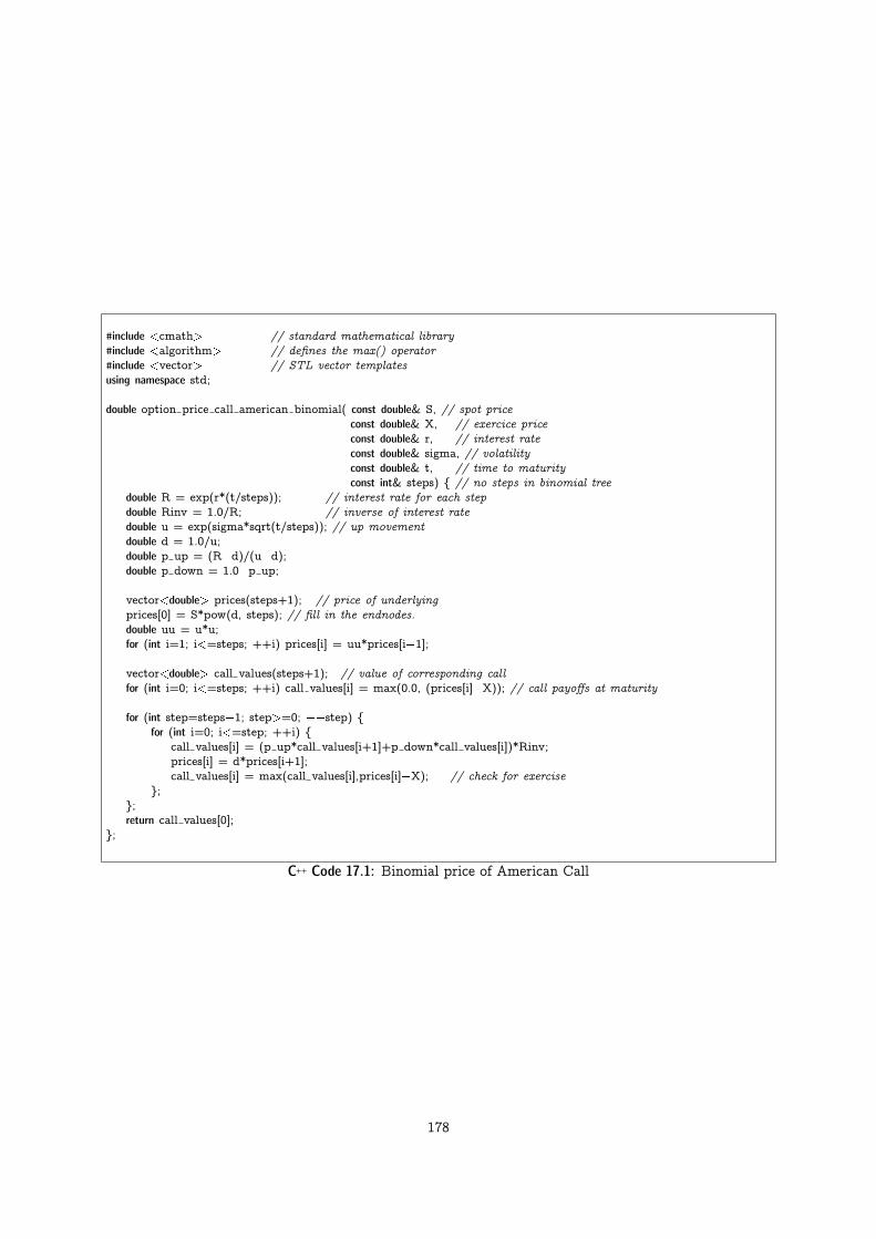
#include <cmath> // standard mathematical library#include <algorithm> // defines the max() operator#include <vector> // STL vector templatesusing namespace std;
double option price call american binomial( const double& S, // spot priceconst double& X, // exercice priceconst double& r, // interest rateconst double& sigma, // volatilityconst double& t, // time to maturityconst int& steps) { // no steps in binomial tree
double R = exp(r*(t/steps)); // interest rate for each stepdouble Rinv = 1.0/R; // inverse of interest ratedouble u = exp(sigma*sqrt(t/steps)); // up movementdouble d = 1.0/u;double p up = (R�d)/(u�d);double p down = 1.0�p up;
vector<double> prices(steps+1); // price of underlyingprices[0] = S*pow(d, steps); // fill in the endnodes.double uu = u*u;for (int i=1; i<=steps; ++i) prices[i] = uu*prices[i�1];
vector<double> call values(steps+1); // value of corresponding callfor (int i=0; i<=steps; ++i) call values[i] = max(0.0, (prices[i]�X)); // call payoffs at maturity
for (int step=steps�1; step>=0; ��step) {for (int i=0; i<=step; ++i) {
call values[i] = (p up*call values[i+1]+p down*call values[i])*Rinv;prices[i] = d*prices[i+1];call values[i] = max(call values[i],prices[i]�X); // check for exercise
};};return call values[0];
};
C++ Code 17.1: Binomial price of American Call
178

#include <cmath> // standard mathematical library#include <algorithm> // defines the max() operator#include <vector> // STL vector templatesusing namespace std;
double option price generic binomial( const double& S,const double& K,double generic payoff(const double& S, const double& K),const double& r,const double& sigma,const double& t,const int& steps) {
double R = exp(r*(t/steps)); // interest rate for each stepdouble Rinv = 1.0/R; // inverse of interest ratedouble u = exp(sigma*sqrt(t/steps)); // up movementdouble d = 1.0/u;double p up = (R�d)/(u�d);double p down = 1.0�p up;
vector<double> prices(steps+1); // price of underlyingprices[0] = S*pow(d, steps); // fill in the endnodes.double uu = u*u;for (int i=1; i<=steps; ++i) prices[i] = uu*prices[i�1];
vector<double> values(steps+1); // value of corresponding callfor (int i=0; i<=steps; ++i) values[i] = generic payoff(prices[i],K); // payoffs at maturity
for (int step=steps�1; step>=0; ��step) {for (int i=0; i<=step; ++i) {
values[i] = (p up*values[i+1]+p down*values[i])*Rinv; // value by not exercisingprices[i] = d*prices[i+1];values[i] = max(values[i],generic payoff(prices[i],K)); // check for exercise
};};return values[0];
};
C++ Code 17.2: Generic binomial calculation
179

Using this routine is then merely a matter of providing a definition of the derivative payoff. C++ Code 17.3shows how the payoffs are defined for standard put and call options. Pricing American put and calloptions is then merely a matter of supplying these payoff definitions to the generic binomial routine.
#include <algorithm>using namespace std;
double payoff call(const double& S, const double& K){return max(0.0,S�K);
};
double payoff put (const double& S, const double& K) {return max(0.0,K�S);
};
C++ Code 17.3: Payoff definitions for put and call options
Example
Consider American call and put option on non-dividend paying stock, where S = 100, K = 100, � = 0:2,(T � t) = 1 and r = 0:1.
1. Price the options using binomial approximations with 100 steps.
C++ program:
double S = 100.0;double K = 100.0;double r = 0.1;double sigma = 0.25;double time to maturity=1.0;int steps = 100;cout << " american call price = "
<< option price generic binomial(S,K,payoff call, r, sigma, time to maturity, steps)<< endl;
cout << " american put price = "<< option price generic binomial(S,K,payoff put, r, sigma, time to maturity, steps)<< endl;
Output from C++ program:
american call price = 14.9505american put price = 6.54691
More exotic options can also be calculated using the same approach. For example, C++ Code 17.4 showspayoff definitions for two binary options, options that pay off one dollar if the price of the underlying isabove K (call) or below K (put). The typical such option is European, the check for whether the optionis in the money happens at maturity, but one can also think of cases where the binary option pays offone dollar as soon as S, the price of the underlying, hits the “barrier” K.
Example
Consider binary options that pays one dollar if the price S of the underlying increases to K or above duringsome time period. Suppose the current price of the underlying is S = 100. Using � = 0:2, (T � t) = 1 andr = 0:1, price such a binary option when K = 120.
180

double payoff binary call(const double& S, const double& K){if (S>=K) return 1;return 0;
};
double payoff binary put(const double& S, const double& K){if (S<=K) return 1;return 0;
};
C++ Code 17.4: Payoff definitions for binomial options
C++ program:
double S = 100.0;double K = 120.0;double r = 0.1;double sigma = 0.25;double time to maturity=1.0;int steps = 100;cout << " binary option price = "
<< option price generic binomial(S,K,payoff binary call, r, sigma, time to maturity, steps)<< endl;
Output from C++ program:
binary option price = 0.498858
181

17.2 Delta calculation
Deltas and other greeks are calculated using the same style of generic routine. C++ Code 17.5 shows howto calculate delta using the same generic approach.
#include <cmath>#include <algorithm>#include <vector>using namespace std;
double option price delta generic binomial(const double& S,const double& K,double generic payoff(const double& S, const double& K),const double& r,const double& sigma,const double& t,const int& no steps){
double R = exp(r*(t/no steps));double Rinv = 1.0/R;double u = exp(sigma*sqrt(t/no steps));double d = 1.0/u;double uu= u*u;double pUp = (R�d)/(u�d);double pDown = 1.0 � pUp;
vector<double> prices (no steps+1);prices[0] = S*pow(d, no steps);for (int i=1; i<=no steps; ++i) prices[i] = uu*prices[i�1];
vector<double> values (no steps+1);for (int i=0; i<=no steps; ++i) values[i] = generic payoff(prices[i],K);
for (int CurrStep=no steps�1 ; CurrStep>=1; ��CurrStep) {for (int i=0; i<=CurrStep; ++i) {
prices[i] = d*prices[i+1];values[i] = (pDown*values[i]+pUp*values[i+1])*Rinv;values[i] = max(values[i], generic payoff(prices[i],K));
};};double delta = (values[1]�values[0])/(S*u�S*d);return delta;
};
C++ Code 17.5: Generic binomial calculation of delta
Exercise 17.1.
The generic routines discussed in this chapter have been for American options. How would you modify themto account for European options?
182

Chapter 18
Trinomial trees
Contents18.1 Intro . . . . . . . . . . . . . . . . . . . . . . . . . . . . . . . . . . . . . . . . . . . . . . . 18318.2 Implementation . . . . . . . . . . . . . . . . . . . . . . . . . . . . . . . . . . . . . . . . . . 18318.3 Further reading . . . . . . . . . . . . . . . . . . . . . . . . . . . . . . . . . . . . . . . . . . 185
18.1 Intro
A trinomial tree is similar to a binomial tree, just with one more branch. At each point of time thereare three possible future values of the underlying S.
S0 ���
�����*
-HHH
HHHHHj
Su = uS0
Sm = S0
Sd = dS0
18.2 Implementation
A trinomial tree can be implemented with various parameterizations. We will show the calulation usingthe following parameterization:
u = e�p3�t
e =1
u
pu = �r
�t
12�2
�r � q � �2
2
�+
1
6
pm =2
3
pu =
r�t
12�2
�r � q � �2
2
�+
1
6
183

We calculate the option price using the usual roll back procedure with the continuation value
e�r�t (pufu + pmfm + pdfd)
#include <vector>#include <cmath>using namespace std;
double option price put american trinomial( const double& S,const double& K,const double& r,const double& q,const double& sigma,const double& t,const int& steps) {
double delta t = t/steps;double Rinv = exp(�r*(delta t));double sigma sqr=pow(sigma,2);
double u = exp(sigma*sqrt(3.0*delta t));double d = 1.0/u;double p u = 1.0/6.0 + sqrt(delta t/(12.0*sigma sqr)) * (r�q�0.5*sigma sqr);double p m = 2.0/3.0;double p d = 1.0/6.0 � sqrt(delta t/(12.0*sigma sqr)) * (r�q�0.5*sigma sqr);
vector< vector<double> > Stree; // price of underlying in a treevector<double> Svec;Svec.push back(S);for (int step=1;step<=steps;++step){
Stree.push back(Svec);Svec.insert(Svec.begin(),Svec[0]*d); // use the fact that only the extreme values change.Svec.push back(Svec[Svec.size()�1]*u);
};int m = int(Svec.size());vector<double> values next = vector<double>(m); // value of option next stepfor (int i=0; i<m; ++i) values next[i] = max(0.0, K�Svec[i]); // call payoffs at maturityvector<double> values;for (int step=steps�1; step>=0; ��step) {
m = int(Stree[step].size());values = vector<double> (m); // value of optionfor (int i=0; i<m; ++i) {
values[i] = (p u*values next[i+2]+p m*values next[i+1] + p d*values next[i])*Rinv;values[i] = max(values[i],K�Stree[step][i]); // check for exercise
};values next=values;
};return values[0];
};
C++ Code 18.1: Price of american put using a trinomial tree
Example
You are given the following information about an option: S = 100, K = 100, r = 0:1, � = 0:25 and time tomaturity is 1 year. Price an American put using a trinomial approximation with 100 steps.
184

function P = opt price trinom am put(S, K, r, q, sigma, t, steps)delta t = t/steps;sigma sqr=sigma^2;Rinv = exp(�r*delta t);u = exp(sigma*sqrt(3.0*delta t));d = 1.0/u;p u = 1/6 + sqrt(delta t/(12*sigma sqr)) * (r�q�0.5*sigma sqr);p m = 2/3;p d = 1/6 � sqrt(delta t/(12*sigma sqr)) * (r�q�0.5*sigma sqr);
Svec = [ S ];Stree = [ Svec ];Su = S;Sd = S;for step=1:steps+1
Su = Su*u;Sd = Sd*d;Svec = [ Sd; Svec; Su ];Stree=[ [Stree; zeros(2,step)] Svec ];
endvalues next = max(0,K�Svec);for step = steps:�1:0
m = 2*step+1;values = Rinv*(p u*values next(3:m+2)+p m*values next(2:m+1)+p d*values next(1:m));values = max(values, K�Stree(1:m,step+1));values next = values;
endendP = values;
end
Matlab Code 18.1: Price of american put using a trinomial tree
C++ program:
double S = 100.0; double K = 100.0;double r = 0.1; double q = 0; double sigma = 0.25;double time=1.0; int no steps = 100;cout << " american put = " << option price put american trinomial(S,K,r,q,sigma,time,no steps) << endl;
Output from C++ program:
american put = 6.52719
Exercise 18.1.
In the code for the trinomial tree the price of the underlying is put into a triangular data structure. This canbe collapsed into a single array, since the only changes when you add one step is to add one price at the topand at the bottom. If you keep track of the top and bottom of the current array you can access the prices ofthe underlying through some clever indexing into the single vector of prices of the underlying.
Exercise 18.2.
Similarly to the binomial case, one can build a generic trinomial tree where the payoff function is passed as aparameter to the routine. Implement such a generic trinomial tree.
18.3 Further reading
Hull (2011)
185

Chapter 19
Alternatives to the Black Scholes type optionformula
Contents19.1 Merton’s Jump diffusion model. . . . . . . . . . . . . . . . . . . . . . . . . . . . . . . . . . . 18619.2 Hestons pricing formula for a stochastic volatility model . . . . . . . . . . . . . . . . . . . . . 188
A large number of alternative formulations to the Black Scholes analysis has been proposed. Few ofthem have seen any widespread use, but we will look at some of these alternatives.
19.1 Merton’s Jump diffusion model.
Merton (1976) has proposed a model where in addition to a Brownian Motion term, the price process ofthe underlying is allowed to have jumps. The risk of these jumps is assumed to not be priced.
In the following we look at an implementation of a special case of Merton’s model, described in (Hull,1993, pg 454), where the size of the jump has a normal distribution. � and � are parameters of thejump distribution. The price of an European call option is given in Formula 19.1 and implemented inC++ Code 19.1
c =
1Xn=0
e�0� (�0� )n
n!CBS(S;X; rn; �
2n; T � t)
where
� = T � t
�0 = �(1 + �)
CBS(�) is the Black Scholes formula, and
�2n = �2 +n�2
�
rn = r � ��+n ln(1 + �)
�
Formula 19.1: The option pricing formula of the Merton (1976) model
In implementing this formula, we need to terminate the infinite sum at some point. But since the
186
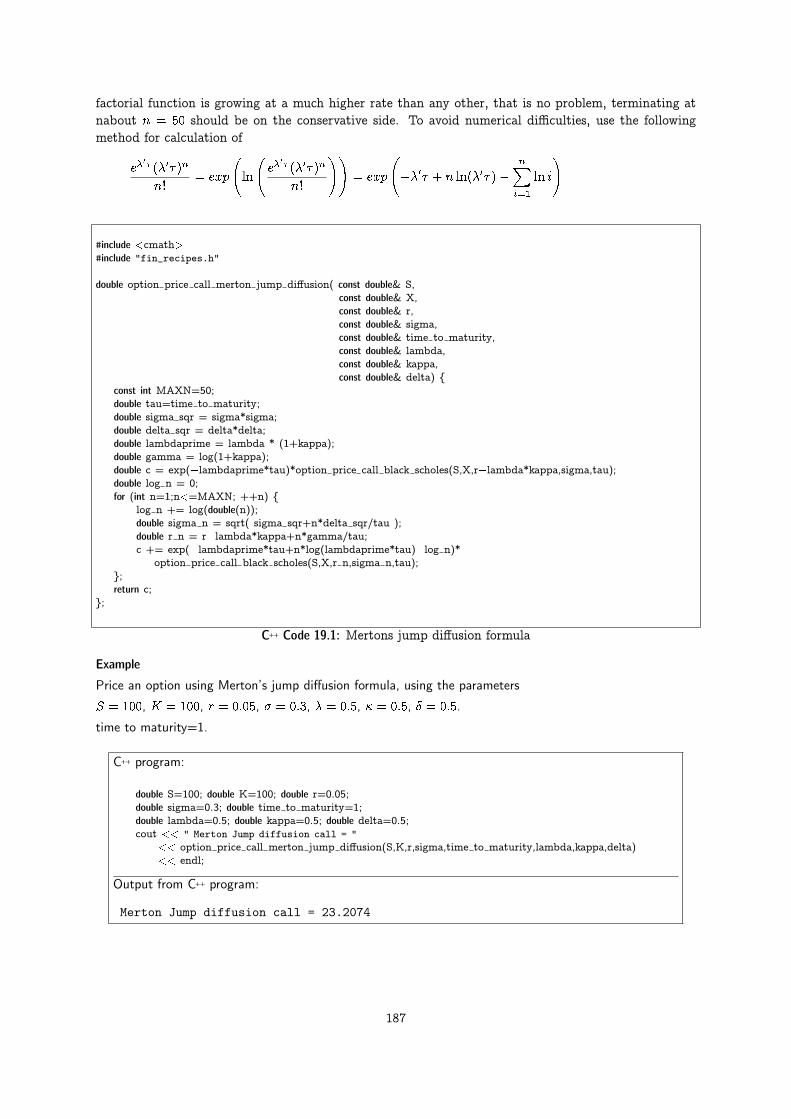
factorial function is growing at a much higher rate than any other, that is no problem, terminating atnabout n = 50 should be on the conservative side. To avoid numerical difficulties, use the followingmethod for calculation of
e�0� (�0� )n
n!= exp
ln
e�
0� (�0� )n
n!
!!= exp
��0� + n ln(�0� )�
nXi=1
ln i
!
#include <cmath>#include "fin_recipes.h"
double option price call merton jump diffusion( const double& S,const double& X,const double& r,const double& sigma,const double& time to maturity,const double& lambda,const double& kappa,const double& delta) {
const int MAXN=50;double tau=time to maturity;double sigma sqr = sigma*sigma;double delta sqr = delta*delta;double lambdaprime = lambda * (1+kappa);double gamma = log(1+kappa);double c = exp(�lambdaprime*tau)*option price call black scholes(S,X,r�lambda*kappa,sigma,tau);double log n = 0;for (int n=1;n<=MAXN; ++n) {
log n += log(double(n));double sigma n = sqrt( sigma sqr+n*delta sqr/tau );double r n = r�lambda*kappa+n*gamma/tau;c += exp(�lambdaprime*tau+n*log(lambdaprime*tau)�log n)*
option price call black scholes(S,X,r n,sigma n,tau);};return c;
};
C++ Code 19.1: Mertons jump diffusion formula
Example
Price an option using Merton’s jump diffusion formula, using the parameters
S = 100, K = 100, r = 0:05, � = 0:3, � = 0:5, � = 0:5, � = 0:5.
time to maturity=1.
C++ program:
double S=100; double K=100; double r=0.05;double sigma=0.3; double time to maturity=1;double lambda=0.5; double kappa=0.5; double delta=0.5;cout << " Merton Jump diffusion call = "
<< option price call merton jump diffusion(S,K,r,sigma,time to maturity,lambda,kappa,delta)<< endl;
Output from C++ program:
Merton Jump diffusion call = 23.2074
187

19.2 Hestons pricing formula for a stochastic volatility model
Heston (1993) relaxes the Black-Scholes assumption of a constant volatility by introducing a stochasticvolatility. He finds exact solutions for European options.
Let S be the stock price and v the volatility. These two variables are assumed to follow joint stochasticprocesses.�
dS(t) = �Sdt+pv(t)Sdz1(t)
dpv(t) = ��
pv(t)dt+ �v(t)Sdz2(t)
�The two processes z1 and z2 have correlation �. Rewrite the process for the volatility as
dv(t) = � (�� v(t)) dt+ �pv(t)dz2
Let �(S; v; t) be the price of volatility risk. Under a constant interest rate r
P (t; T ) = e�r(T�t)
Consider a call option with strike price K. Its price is given by Formula 19.2.
Price of Call option using Hestons formula The option price is
C(s; v; t) = SP1 �KP (t; T )P2
where
Pj(x; v; T; ln(K)) =1
2+
1
�
Z 1
0
Re
�e�i� ln(K)fj(x; v; T; �)
i�d�
�fj(x; v; T; �) = eC(�;�)+D(�;�)v+i�x
C(�; �) = r�i� +a
�2
�(bj � ���i+ d)� � 2 ln
�1� ged�
1� g
��
D(�; �) =bj � ���i+ d
�2
�1� ed�
1� ged�
�
u1 =1
2; u2 = �1
2
a = ��
b1 = �+ �� �� b2 = �+ �
x = ln(S)
g =bj � ���i+ d
bj � ���i� d
d =q(���i� bj)2 � �2(2uj�i� �2)
Notation: S: price of undelying security. K: exercise price.
The implementation of this pricing formula has some instructive C++ features. First, it illustrates cal-culations of of complex variables. Complex numbers is part of the C++ standard, and are accessed byincluding the
#include <complex>
188

statement. Complex numbers are templated, it is necessary to specify what type of floating point typeto use, such as complex<double> or complex<double double>.
To evaluate the price it is also necessary to do a numerical integration. In the calculation this is solvedby a call to an external routine. We use a routine provided by the Gnu GSL project.1
Example
Given the following set of parameters: S = 100, K = 100, r = 0:01, v = 0:01, � = 0:5, � = 0, � = 2, � = 0,� = 0:01 and � = 0:01, price a call option using the Heston formula
C++ program:
double S=100; double K=100; double r=0.01; double v=0.01;double tau=0.5; double rho=0; double kappa=2; double lambda=0.0;double theta=0.01; double sigma=0.01;cout << "heston call price "
<< heston call option price( S, K, r, v, tau, rho, kappa, lambda, theta, sigma) << endl;
Output from C++ program:
heston call price 3.06944
1An example alternatives would have been Numerical Recipes in C++’s quadrature.
189

#include <iostream>#include <cmath>#include <complex>using namespace std;#include "gsl/gsl_integration.h"
struct heston parms {double K; double x; double r; double v; double tau; double kappa; double theta;double rho; double sigma; double lambda; int j;};
extern "C"{double heston integrand j(double phi, void *p){
struct heston parms* parms = (struct heston parms*)p;double K = (parms�>K); double x = (parms�>x);double v = (parms�>v); double r = (parms�>r);double kappa = (parms�>kappa);double theta = (parms�>theta);double rho = (parms�>rho);double sigma = (parms�>sigma);double lambda = (parms�>lambda);double tau = (parms�>tau);double j = (parms�>j);double sigma sqr = pow(sigma,2);double uj; double bj;if (j==1){ uj=0.5; bj=kappa+lambda�rho*sigma; }else { uj=�0.5; bj=kappa+lambda; };complex <double> i(0,1);double a = kappa*theta;complex<double> d = sqrt( pow(rho*sigma*phi*i�bj,2) � sigma sqr*(2*uj*phi*i�pow(phi,2)) );complex<double> g = (bj � rho*sigma*phi*i+d)/(bj�rho*sigma*phi*i�d);complex<double> C = r*phi*i*tau+(a/sigma sqr)*((bj�rho*sigma*phi*i+d)*tau�2.0*log((1.0�g*exp(d*tau))/(1.0�g)));complex<double> D = (bj�rho*sigma*phi*i+d)/sigma sqr * ( (1.0�exp(d*tau))/(1.0�g*exp(d*tau)) );complex<double> f1 = exp(C+D*v+i*phi*x);complex<double> F = exp(�phi*i*log(K))*f1/(i*phi);return real(F);
};};
inline double heston Pj(double S, double K, double r, double v, double tau, double sigma,double kappa, double lambda, double rho, double theta, int j){
double x=log(S);struct heston parms parms = { K, x, r, v, tau, kappa, theta, rho, sigma, lambda, j};size t n=10000;gsl integration workspace* w = gsl integration workspace alloc(n);gsl function F;F.function = &heston integrand j;F.params=&parms;double result, error;gsl integration qagiu(&F,0,1e�7,1e�7,n,w,&result,&error); // integral to infinity starting at zeroreturn 0.5 + result/M PI;
};
double heston call option price(const double& S, const double& K, const double& r, const double& v,const double& tau, const double& rho, const double& kappa,const double& lambda, const double& theta, const double& sigma){
double P1 = heston Pj(S,K,r,v,tau,sigma,kappa,lambda,rho,theta,1);double P2 = heston Pj(S,K,r,v,tau,sigma,kappa,lambda,rho,theta,2);double C=S*P1�K*exp(�r*tau)*P2;return C;
};
C++ Code 19.2: Hestons pricing formula for a stochastic volatility model
190
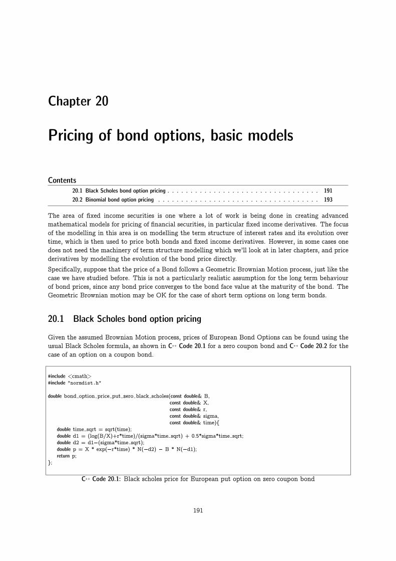
Chapter 20
Pricing of bond options, basic models
Contents20.1 Black Scholes bond option pricing . . . . . . . . . . . . . . . . . . . . . . . . . . . . . . . . . 19120.2 Binomial bond option pricing . . . . . . . . . . . . . . . . . . . . . . . . . . . . . . . . . . . 193
The area of fixed income securities is one where a lot of work is being done in creating advancedmathematical models for pricing of financial securities, in particular fixed income derivatives. The focusof the modelling in this area is on modelling the term structure of interest rates and its evolution overtime, which is then used to price both bonds and fixed income derivatives. However, in some cases onedoes not need the machinery of term structure modelling which we’ll look at in later chapters, and pricederivatives by modelling the evolution of the bond price directly.
Specifically, suppose that the price of a Bond follows a Geometric Brownian Motion process, just like thecase we have studied before. This is not a particularly realistic assumption for the long term behaviourof bond prices, since any bond price converges to the bond face value at the maturity of the bond. TheGeometric Brownian motion may be OK for the case of short term options on long term bonds.
20.1 Black Scholes bond option pricing
Given the assumed Brownian Motion process, prices of European Bond Options can be found using theusual Black Scholes formula, as shown in C++ Code 20.1 for a zero coupon bond and C++ Code 20.2 for thecase of an option on a coupon bond.
#include <cmath>#include "normdist.h"
double bond option price put zero black scholes(const double& B,const double& X,const double& r,const double& sigma,const double& time){
double time sqrt = sqrt(time);double d1 = (log(B/X)+r*time)/(sigma*time sqrt) + 0.5*sigma*time sqrt;double d2 = d1�(sigma*time sqrt);double p = X * exp(�r*time) * N(�d2) � B * N(�d1);return p;
};
C++ Code 20.1: Black scholes price for European put option on zero coupon bond
191

#include <cmath>#include <vector>using namespace std;#include "normdist.h"#include "fin_recipes.h"
double bond option price put coupon bond black scholes( const double& B,const double& X,const double& r,const double& sigma,const double& time,const vector<double> coupon times,const vector<double> coupon amounts){
double adjusted B=B;for (unsigned int i=0;i<coupon times.size();i++) {
if (coupon times[i]<=time) {adjusted B �= coupon amounts[i] * exp(�r*coupon times[i]);
};};return bond option price put zero black scholes(adjusted B,X,r,sigma,time);
};
C++ Code 20.2: Black scholes price for European put option on coupon bond
192

20.2 Binomial bond option pricing
Since we are in the case of geometric Brownian motion, the usual binomial approximation can be used toprice American options, where the bond is the underlying security. C++ Code 20.3 shows the calculationof a put price
#include <cmath> // standard mathematical library#include <algorithm> // defining the max() operator#include <vector> // STL vector templatesusing namespace std;
double bond option price put american binomial( const double& B, // Bond priceconst double& K, // exercise priceconst double& r, // interest rateconst double& sigma, // volatilityconst double& t, // time to maturityconst int& steps){ // no steps in binomial tree
double R = exp(r*(t/steps)); // interest rate for each stepdouble Rinv = 1.0/R; // inverse of interest ratedouble u = exp(sigma*sqrt(t/steps)); // up movementdouble uu = u*u;double d = 1.0/u;double p up = (R�d)/(u�d);double p down = 1.0�p up;vector<double> prices(steps+1); // price of underlyingvector<double> put values(steps+1); // value of corresponding put
prices[0] = B*pow(d, steps); // fill in the endnodes.for (int i=1; i<=steps; ++i) prices[i] = uu*prices[i�1];for (int i=0; i<=steps; ++i) put values[i] = max(0.0, (K�prices[i])); // put payoffs at maturityfor (int step=steps�1; step>=0; ��step) {
for (int i=0; i<=step; ++i) {put values[i] = (p up*put values[i+1]+p down*put values[i])*Rinv;prices[i] = d*prices[i+1];put values[i] = max(put values[i],(K�prices[i])); // check for exercise
};};return put values[0];
};
C++ Code 20.3: Binomial approximation to american put bond option price
193

Example
Parameters: B = 100, K = 100, r = 0:05, � = 0:1, time=1.
There is also a coupon bond with the the same bond price, but paying coupon of 0:5 at date 1.
1. Price a an European put option on the zero coupon bond using Black Scholes.
2. Price a an European put option on the coupon coupon bond using Black Scholes.
3. Price a an European put option on the zero coupon bond using binomial approximation with 100 steps.
C++ program:
double B=100;double K=100;double r=0.05;double sigma=0.1;double time=1;cout << " zero coupon put option price = "
<< bond option price put zero black scholes(B,K,r,sigma,time) << endl;
vector<double> coupon times; coupon times.push back(0.5);vector<double> coupons; coupons.push back(1);cout << " coupon bond put option price = "
<< bond option price put coupon bond black scholes(B,K,r,sigma,time,coupon times,coupons);cout << endl;
int steps=100;cout << " zero coupon american put option price, binomial = "
<< bond option price put american binomial(B,K,r,sigma,time,steps) << endl;
Output from C++ program:
zero coupon put option price = 1.92791coupon bond put option price = 2.22852zero coupon american put option price, binomial = 2.43282
194

Chapter 21
Credit risk
Contents21.1 The Merton Model . . . . . . . . . . . . . . . . . . . . . . . . . . . . . . . . . . . . . . . . 19521.2 Issues in implementation . . . . . . . . . . . . . . . . . . . . . . . . . . . . . . . . . . . . . 196
Option pricing has obvious applications to the pricing of risky bonds.
21.1 The Merton Model
This builds on the Black and Scholes (1973) and Merton (1973) framework to find the value of the debtissued by the firm. The ideas were already in Black and Scholes, who discussed the view of the firm asa call option.
Assume debt structure: There is a single debt issue. Debt is issued as a zero coupon bond. The bond isdue on a given date T .
Assuming the firm value V follows the usual Brownian motion proces, debt is found as a closed formsolution, similar in structure to the Black Scholes equation for a call option.
Easiest seen from the interpretation of firm debt as the price of risk free debt, minus the value of a putoption.
Price debt by the price B of risk free debt, and then subtract the price of the put, using the BlackScholes formula.
The Black Scholes formula for a call option is
c = S �N(d1)�K � e�r(T�t)N(d2)
where
d1 =ln�SK
�+ (r + 1
2�)(T � t)
�pT � t
d2 = d1 � �pT � t
N(�) = The cumulative normal distribution
p = Ke�r(T�t)N(�d2)� SN(�d1)
In the context here, reinterpret S as V , firm value. The put is priced as
p = Ke�r(T�t)N(�d2)� VtN(�d1)
195

where
d1 =ln�VtK
�+ (r + 1
2�)(T � t)
�pT � t
Note on interpretation: The spread between risky and risk free debt determined solely by the price ofthe put option.
Example
The current value of the firm V = 100. The firm has issued one bond with face value 90, which is due tobe paid one year from now. The risk free interest rate is 5% and the volatility of the firms value is 25%.Determine the value of the debt.
C++ program:
cout << " Credit Risk Calculation " << endl;double V=100; double F=90; double r=0.05; double T=1; double sigma=0.25;double p = option price put black scholes(V,F,r,sigma,T);cout << " Debt value = " << exp(�r*T)*F � p << endl;
Output from C++ program:
Credit Risk CalculationDebt value = 81.8592
21.2 Issues in implementation
� Firm value and firm volatility is unobservable.
� The model assumes a simple debt structure, most debt structures tend to be more complex.
196

Chapter 22
Term Structure Models
Contents22.1 The Nelson Siegel term structure approximation . . . . . . . . . . . . . . . . . . . . . . . . . 19822.2 Extended Nelson Siegel models . . . . . . . . . . . . . . . . . . . . . . . . . . . . . . . . . . 20022.3 Cubic spline. . . . . . . . . . . . . . . . . . . . . . . . . . . . . . . . . . . . . . . . . . . . 20222.4 Cox Ingersoll Ross. . . . . . . . . . . . . . . . . . . . . . . . . . . . . . . . . . . . . . . . . 20522.5 Vasicek . . . . . . . . . . . . . . . . . . . . . . . . . . . . . . . . . . . . . . . . . . . . . . 20822.6 Readings . . . . . . . . . . . . . . . . . . . . . . . . . . . . . . . . . . . . . . . . . . . . . 210
We now expand on the analysis of the term structure in chapter 5. As shown there, the term structureis best viewed as an abstract class providing, as functions of term to maturity, the prices of zero couponbonds (discount factors), yield on zero coupon bonds (spot rates) or forward rates. In the earlier casewe considered two particular implementations of the term structure: A flat term structure or a termstructure estimated by linear interpolations of spot rates. We now consider a number of alternative termstructure models. The focus of this chapter is empirical, we consider ways in which on one can specify aterm structure in a lower dimensional way. Essentially we are looking at ways of doing curve-fitting, ofestimating a nonlinear relationship between time and discount factors, or between time and spot rates.Since the relationship is nonlinear, this is a nontrivial problem. One has to choose a functional form toestimate, which allows enough flexibility to “fit” the term structure, but not so flexible that it violatesthe economic restrictions on the term structure. Here are some considerations.
� Discount factors must be positive. (dt > 0). This is because they are prices, negative prices allowfor abritrage.
� Discount factors must be a nonincreasing function of time. (dt � dt+k 8 k > 0). Again, this is toavoid arbitrage.
� Nominal interest rates can not be negative. (rt � 0 8 t) This is another implication of the absenceof arbitrage opportunities.
� Both discount factors and interest rates must be smooth functions of time.
� The value of a payment today is the payment today. d0 = 1.
A number of alternative ways of estimating the term structure has been considered. Some are purelyused as interpolation functions, while others are fully specified, dynamic term structure models. Ofthe models that follow, the approximating function proposed in Nelson and Siegel (1987) and the cubicspline used by e.g. McCulloch (1971) are examples of the first kind, and the term structure models ofCox, Ingersoll, and Ross (1985) and Vasicek (1977) are examples of the second kind.
197
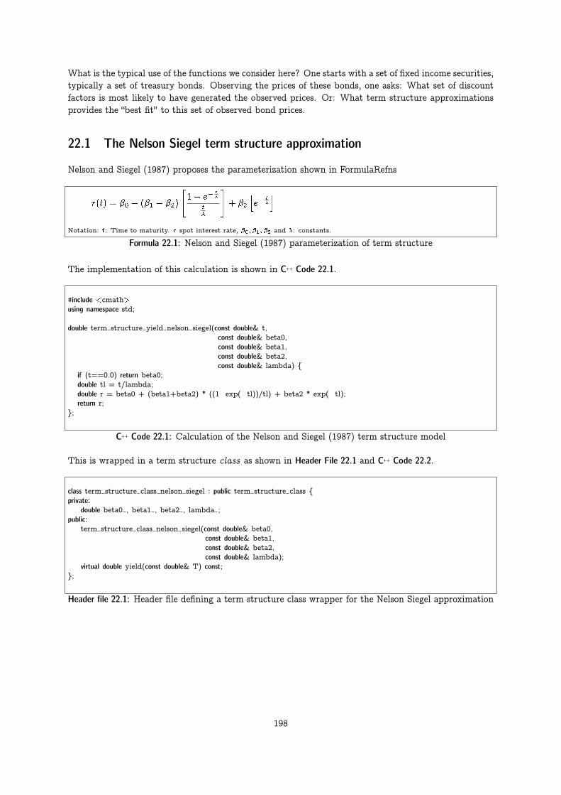
What is the typical use of the functions we consider here? One starts with a set of fixed income securities,typically a set of treasury bonds. Observing the prices of these bonds, one asks: What set of discountfactors is most likely to have generated the observed prices. Or: What term structure approximationsprovides the “best fit” to this set of observed bond prices.
22.1 The Nelson Siegel term structure approximation
Nelson and Siegel (1987) proposes the parameterization shown in FormulaRefns
r(t) = �0 + (�1 + �2)
"1� e�
t�
t�
#+ �2
he�
t�
iNotation: t: Time to maturity. r spot interest rate, �0; �1; �2 and �: constants.
Formula 22.1: Nelson and Siegel (1987) parameterization of term structure
The implementation of this calculation is shown in C++ Code 22.1.
#include <cmath>using namespace std;
double term structure yield nelson siegel(const double& t,const double& beta0,const double& beta1,const double& beta2,const double& lambda) {
if (t==0.0) return beta0;double tl = t/lambda;double r = beta0 + (beta1+beta2) * ((1�exp(�tl))/tl) + beta2 * exp(�tl);return r;
};
C++ Code 22.1: Calculation of the Nelson and Siegel (1987) term structure model
This is wrapped in a term structure class as shown in Header File 22.1 and C++ Code 22.2.
class term structure class nelson siegel : public term structure class {private:
double beta0 , beta1 , beta2 , lambda ;public:
term structure class nelson siegel(const double& beta0,const double& beta1,const double& beta2,const double& lambda);
virtual double yield(const double& T) const;};
Header file 22.1: Header file defining a term structure class wrapper for the Nelson Siegel approximation
198

#include "fin_recipes.h"
term structure class nelson siegel::term structure class nelson siegel( const double& b0,const double& b1,const double& b2,const double& l) {
beta0 =b0; beta1 =b1; beta2 =b2; lambda =l;};
double term structure class nelson siegel::r(const double& t) const {if (t<=0.0) return beta0 ;return term structure yield nelson siegel(t,beta0 ,beta1 ,beta2 ,lambda );
};
C++ Code 22.2: Defining a term structure class wrapper for the Nelson Siegel approximation
199

Example
Using the parameters �0 = 0:01, �1 = 0:01, �2 = 0:01, � = 5:0 and t = 1 in the Nelson Siegel approximation,find the 1 year discount factor and spot rate, and the forward rate between years 1 and 2.
C++ program:
double beta0=0.01; double beta1=0.01; double beta2=0.01; double lambda=5.0;double t=1.0;cout << "Example calculations using the Nelson Siegel term structure approximation"
<< endl;cout << " direct calculation, yield = "
<< term structure yield nelson siegel(t,beta0,beta1,beta2,lambda) << endl;term structure class nelson siegel ns(beta0,beta1,beta2,lambda);cout << " using a term structure class" << endl;cout << " yield (t=1) = " << ns.r(t) << endl;cout << " discount factor (t=1) = " << ns.d(t) << endl;cout << " forward rate (t1=1, t2=2) = " << ns.f(1,2) << endl;
Output from C++ program:
Example calculations using the Nelson Siegel term structure approximationdirect calculation, yield = 0.0363142using a term structure classyield (t=1) = 0.0363142discount factor (t=1) = 0.964337forward rate (t1=1, t2=2) = 0.0300602
22.2 Extended Nelson Siegel models
The Nelson and Siegel (1987) model is simple, with parameters with clear obvious economic interpre-tations. It does have the problem that the term structure shapes that it allows is limited. To allowfor more complex shapes, such as humped shapes, it has been extended in various ways. A popularapproximation was introduced by Lars Svensson, parameterized as shown in Formula 22.2
r(t) = �0 + �1
1� e�
t�1
t�
!+ �2
1� e�
t�1
t�1
� e�t�1
!+ �3
1� e�
t�2
t�2
� e�t�2
!Notation: t: Time to maturity. r spot interest rate, �0; �1; �2 and �: constants.
Formula 22.2: Svensson’s extension of the Nelson and Siegel (1987) parameterization of term structure
This is wrapped in a term structure class as shown in Header File 22.2 and C++ Code 22.4.
200

#include <cmath>using namespace std;
double term structure yield svensson(const double& t,const double& beta0,const double& beta1,const double& beta2,const double& beta3,const double& tau1,const double& tau2){
if (t==0.0) return beta0;double r = beta0;r += beta1* ((1�exp(�t/tau1))/(t/tau1)) ;r += beta2 * ( ((1�exp(�t/tau1))/(t/tau1)) � exp(�t/tau1) );r += beta3 * ( ((1�exp(�t/tau2))/(t/tau2)) � exp(�t/tau2) );return r;
};
C++ Code 22.3: Calculation of Svensson’s extended Nelson and Siegel (1987) term structure model
class term structure class svensson:public term structure class {private:
double beta0 , beta1 , beta2 , beta3 , tau1 , tau2 ;public:
term structure class svensson(const double& beta0,const double& beta1,const double& beta2,const double& beta3,const double& tau1,const double& tau2);
virtual double yield(const double& T) const;};
Header file 22.2: Header file defining a term structure class wrapper for the Svensson model
#include "fin_recipes.h"
term structure class svensson::term structure class svensson( const double& b0, const double& b1, const double& b2, const double& b3,const double& tau1, const double& tau2) {
beta0 =b0; beta1 =b1; beta2 =b2; beta3 =b3; tau1 =tau1; tau2 =tau2;};
double term structure class svensson::r(const double& t) const {if (t<=0.0) return beta0 ;return term structure yield svensson(t,beta0 ,beta1 ,beta2 ,beta3 ,tau1 ,tau2 );
};
C++ Code 22.4: Defining a term structure class wrapper for the Svensson model
201
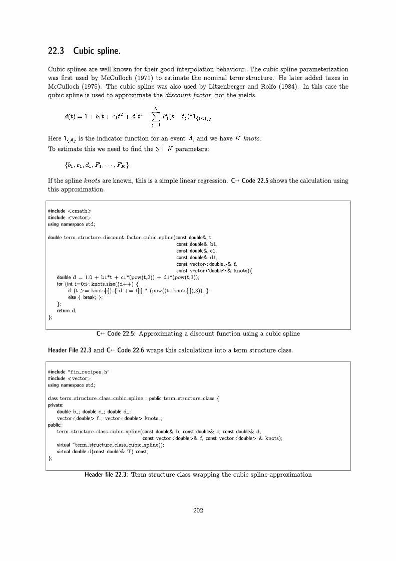
22.3 Cubic spline.
Cubic splines are well known for their good interpolation behaviour. The cubic spline parameterizationwas first used by McCulloch (1971) to estimate the nominal term structure. He later added taxes inMcCulloch (1975). The cubic spline was also used by Litzenberger and Rolfo (1984). In this case thequbic spline is used to approximate the discount factor, not the yields.
d(t) = 1 + b1t+ c1t2 + d1t
3 +
KXj=1
Fj(t� tj)31ft<tjg
Here 1fAg is the indicator function for an event A, and we have K knots .
To estimate this we need to find the 3 +K parameters:
fb1; c1; d1; F1; � � � ; FKg
If the spline knots are known, this is a simple linear regression. C++ Code 22.5 shows the calculation usingthis approximation.
#include <cmath>#include <vector>using namespace std;
double term structure discount factor cubic spline(const double& t,const double& b1,const double& c1,const double& d1,const vector<double>& f,const vector<double>& knots){
double d = 1.0 + b1*t + c1*(pow(t,2)) + d1*(pow(t,3));for (int i=0;i<knots.size();i++) {
if (t >= knots[i]) { d += f[i] * (pow((t�knots[i]),3)); }else { break; };
};return d;
};
C++ Code 22.5: Approximating a discount function using a cubic spline
Header File 22.3 and C++ Code 22.6 wraps this calculations into a term structure class.
#include "fin_recipes.h"#include <vector>using namespace std;
class term structure class cubic spline : public term structure class {private:
double b ; double c ; double d ;vector<double> f ; vector<double> knots ;
public:term structure class cubic spline(const double& b, const double& c, const double& d,
const vector<double>& f, const vector<double> & knots);virtual ˜term structure class cubic spline();virtual double d(const double& T) const;
};
Header file 22.3: Term structure class wrapping the cubic spline approximation
202

#include "fin_recipes.h"
term structure class cubic spline::term structure class cubic spline ( const double& b, const double& c, const double& d,
const vector<double>& f, const vector<double>& knots) {b = b; c = c; d = d; f .clear(); knots .clear();if (f.size()!=knots.size()){ return; };for (int i=0;i<f.size();++i) {
f .push back(f[i]);knots .push back(knots[i]);
};};
double term structure class cubic spline::d(const double& T) const {return term structure discount factor cubic spline(T,b ,c ,d ,f ,knots );
};
C++ Code 22.6: Term structure class wrapping the cubic spline approximation
203

Example
Using the parameters b = 0:1 c = 0:1, d = �0:1,
f =
24 0:01
0:01
�0:01
35
knots =
24 2
7
12
35Find short rates and discount factors for 1 year, and the forward rate between 1 and 2 years.
C++ program:
cout << "Example term structure calculations using a cubic spline " << endl;double b=0.1; double c=0.1; double d=�0.1;vector<double> f; f.push back(0.01); f.push back(0.01); f.push back(�0.01);vector<double> knots; knots.push back(2); knots.push back(7); knots.push back(12);cout << " direct calculation, discount factor (t=1) "
<< term structure discount factor cubic spline(1,b,c,d,f,knots) << endl;cout << " Using a term structure class " << endl;term structure class cubic spline cs(b,c,d,f,knots);cout << " yield (t=1) = " << cs.r(1) << endl;cout << " discount factor (t=1) = " << cs.d(1) << endl;cout << " forward (t1=1, t2=2) = " << cs.f(1,2) << endl;
Output from C++ program:
Example term structure calculations using a cubic splinedirect calculation, discount factor (t=1) 1.1Using a term structure classyield (t=1) = -0.0953102discount factor (t=1) = 1.1forward (t1=1, t2=2) = 0.318454
204

22.4 Cox Ingersoll Ross.
The Cox et al. (1985) model is the best known example of a continuous time, general equilibrium modelof the term structure. It is commonly used in academic work because it is a general equilibrium modelthat still is “simple enough” to let us find closed form expressions for derivative securities.
The short interest rate.
dr(t) = �(� � r(t))dt+ �pr(t)dW
The discount factor for a payment at time T.
d(t; T ) = A(t; T )e�B(t;T )r(t)
where
=p(�+ �)2 + 2�2
A(t; T ) =
"2 e
12 (�+�+ )(T�t)
( + �+ �)(e�(T�t) � 1) + 2
# 2��
�2
and
B(t; T ) =2e (T�t) � 1
( + �+ �)(e�(T�t) � 1) + 2
Five parameters: r, the short term interest rate, �, the mean reversion parameter, �, the “market” riskparameter, � the long–run mean of the process and �, the variance rate of the process.
#include <cmath>using namespace std;
double term structure discount factor cir(const double& t,const double& r,const double& kappa,const double& lambda,const double& theta,const double& sigma){
double sigma sqr=pow(sigma,2);double gamma = sqrt(pow((kappa+lambda),2)+2.0*sigma sqr);double denum = (gamma+kappa+lambda)*(exp(gamma*t)�1)+2*gamma;double p=2*kappa*theta/sigma sqr;double enum1= 2*gamma*exp(0.5*(kappa+lambda+gamma)*t);double A = pow((enum1/denum),p);double B = (2*(exp(gamma*t)�1))/denum;double dfact=A*exp(�B*r);return dfact;
};
C++ Code 22.7: Calculation of the discount factor using the Cox et al. (1985) model
205

#include "fin_recipes.h"
class term structure class cir : public term structure class {private:
double r ; // interest ratedouble kappa ; // mean reversion parameterdouble lambda ; // risk aversiondouble theta ; // long run meandouble sigma ; // volatility
public:˜term structure class cir();term structure class cir(const double& r, const double& k, const double& l,
const double& th, const double& sigma);virtual double d(const double& T) const;
};
Header file 22.4: Class definition, Cox et al. (1985) model, header file
#include "fin_recipes.h"
//term structure class cir::˜term structure class cir(){;};
term structure class cir::term structure class cir(const double& r, const double& k, const double& l,const double& th, const double& sigma) {
r =r; kappa =k; lambda =l; theta =th; sigma =sigma;};
double term structure class cir::d(const double& T) const{return term structure discount factor cir(T,r ,kappa ,lambda ,theta ,sigma );
};
C++ Code 22.8: Class definition, Cox et al. (1985) model
206

Example
Parameters: r = 0:05, � = 0:01, � = 0:1, � = 0:08 and � = 0:0. Use the CIR term structure model. Findshort rate and discount factor for t = 1, and forward rate between years 1 and 2.
C++ program:
cout << "Example calculations using the Cox Ingersoll Ross term structure model " << endl;double r = 0.05; double kappa=0.01; double sigma=0.1; double theta=0.08; double lambda=0.0;cout << " direct calculation, discount factor (t=1): "
<< term structure discount factor cir(1, r, kappa, lambda, theta, sigma) << endl;cout << " using a class " << endl;term structure class cir cir(r,kappa,lambda,theta,sigma);cout << " yield (t=1) = " << cir.r(1) << endl;cout << " discount factor (t=1) = " << cir.d(1) << endl;cout << " forward (t1=1, t2=2) = " << cir.f(1,2) << endl;
Output from C++ program:
Example calculations using the Cox Ingersoll Ross term structure modeldirect calculation, discount factor (t=1): 0.951166using a classyield (t=1) = 0.0500668discount factor (t=1) = 0.951166forward (t1=1, t2=2) = 0.0498756
207

22.5 Vasicek
#include <cmath>using namespace std;
double term structure discount factor vasicek(const double& time,const double& r,const double& a,const double& b,const double& sigma){
double A,B;double sigma sqr = sigma*sigma;double aa = a*a;if (a==0.0){
B = time;A = exp(sigma sqr*pow(time,3))/6.0;
}else {
B = (1.0 � exp(�a*time))/a;A = exp( ((B�time)*(aa*b�0.5*sigma sqr))/aa �((sigma sqr*B*B)/(4*a)));
};double dfact = A*exp(�B*r);return dfact;
}
C++ Code 22.9: Calculating a discount factor using the Vasicek functional form
#include "fin_recipes.h"
class term structure class vasicek : public term structure class {private:
double r ; double a ; double b ; double sigma ;public:
term structure class vasicek(const double& r, const double& a, const double& b, const double& sigma);virtual double discount factor(const double& T) const;
};
Header file 22.5: Class definition, Vasicek (1977) model
208

#include "fin_recipes.h"
term structure class vasicek::term structure class vasicek(const double& r, const double& a,const double& b, const double& sigma) {
r =r; a =a; b =b; sigma =sigma;};
double term structure class vasicek::d(const double& T) const{return term structure discount factor vasicek(T,r ,a ,b ,sigma );
};
C++ Code 22.10: Class definition, Vasicek (1977) model
209

Example
Parameters r = 0:05, a = �0:1, b = 0:1, � = 0:1 Use the Vasicek term structure model. Find short rate anddiscount factor for t = 1, and forward rate between years 1 and 2.
C++ program:
cout << "Example term structure calculation using the Vasicek term structure model"<< endl;
double r=0.05; double a=�0.1; double b=0.1; double sigma=0.1;cout << " direct calculation, discount factor (t=1): "
<< term structure discount factor vasicek(1, r, a, b, sigma) << endl;term structure class vasicek vc(r,a,b,sigma);cout << " using a term structure class " << endl;cout << " yield (t=1) = " << vc.r(1) << endl;cout << " discount factor (t=1) = " << vc.d(1) << endl;cout << " forward rate (t1=1, t2=2) = " << vc.f(1,2) << endl;
Output from C++ program:
Example term structure calculation using the Vasicek term structure modeldirect calculation, discount factor (t=1): 0.955408using a term structure classyield (t=1) = 0.0456168discount factor (t=1) = 0.955408forward rate (t1=1, t2=2) = 0.0281476
22.6 Readings
The methods in this chapter I first studied in my dissertation at Carnegie Mellon University in 1992,which lead to the paper published as Green and Ødegaard (1997). A textbook treatment of estimationand fitting of term structure models can be found in (Martinelli, Priaulet, and Priaulet, 2003, Ch 4)
210

Chapter 23
Binomial Term Structure models
Contents23.1 The Rendleman and Bartter model . . . . . . . . . . . . . . . . . . . . . . . . . . . . . . . . 21123.2 Readings . . . . . . . . . . . . . . . . . . . . . . . . . . . . . . . . . . . . . . . . . . . . . 213
Pricing bond options with the Black Scholes model, or its binomial approximation, as done in chapter 20,does not always get it right. For example, it ignores the fact that at the maturity of the bond, the bondvolatility is zero. The bond volatility decreases as one gets closer to the bond maturity. This behaviouris not captured by the assumptions underlying the Black Scholes assumption. We therefore look at morecomplicated term structure models, the unifying theme of which is that they are built by building treesof the interest rate.
23.1 The Rendleman and Bartter model
The Rendleman and Bartter approach to valuation of interest rate contingent claims (see Rendlemanand Bartter (1979) and Rendleman and Bartter (1980)) is a particular simple one. Essentially, it isto apply the same binomial approach that is used to approximate options in the Black Scholes world,but the random variable is now the interest rate. This has implications for multiperiod discounting:Taking the present value is now a matter of choosing the correct sequence of spot rates, and it maybe necessary to keep track of the whole “tree” of interest rates. Such a tree can then be used to pricevarious fixed income securities. In the next chapter we illustrate this more generally, here we show adirect implementation of the original model. C++ Code 23.1 implements the original algorithm for a calloption on a (long maturity) zero coupon bond.
211

#include <cmath>#include <algorithm>#include <vector>using namespace std;
double bond option price call zero american rendleman bartter(const double& X,const double& option maturity,const double& S,const double& M, // term structure paramtersconst double& interest, // current short interest rateconst double& bond maturity, // time to maturity for underlying bondconst double& maturity payment,const int& no steps) {
double delta t = bond maturity/no steps;
double u=exp(S*sqrt(delta t));double d=1/u;double p up = (exp(M*delta t)�d)/(u�d);double p down = 1.0�p up;
vector<double> r(no steps+1);r[0]=interest*pow(d,no steps);double uu=u*u;for (int i=1;i<=no steps;++i){ r[i]=r[i�1]*uu;};vector<double> P(no steps+1);for (int i=0;i<=no steps;++i){ P[i] = maturity payment; };int no call steps=int(no steps*option maturity/bond maturity);for (int curr step=no steps;curr step>no call steps;��curr step) {
for (int i=0;i<curr step;i++) {r[i] = r[i]*u;P[i] = exp(�r[i]*delta t)*(p down*P[i]+p up*P[i+1]);
};};vector<double> C(no call steps+1);for (int i=0;i<=no call steps;++i){ C[i]=max(0.0,P[i]�X); };for (int curr step=no call steps;curr step>=0;��curr step) {
for (int i=0;i<curr step;i++) {r[i] = r[i]*u;P[i] = exp(�r[i]*delta t)*(p down*P[i]+p up*P[i+1]);C[i]=max(P[i]�X, exp(�r[i]*delta t)*(p up*C[i+1]+p down*C[i]));
};};return C[0];
};
C++ Code 23.1: RB binomial model for European call on zero coupon bond
212

Example
Parameters:K = 950, S = 0:15 and M = 0:05 The interest rate is 10%, The option matures in 4 years, thebond matures in year 5, with a bond maturity payment of 1000. Price the option on the zero coupon bondusing a Randleman–Bartter approximation with 100 steps.
C++ program:
double K=950; double S=0.15; double M=0.05; double interest=0.10;double option maturity=4; double bond maturity=5; double bond maturity payment=1000;int no steps=100;cout << " Rendleman Bartter price of option on zero coupon bond: ";cout << bond option price call zero american rendleman bartter( K, option maturity, S, M,
interest, bond maturity,bond maturity payment, no steps);
Output from C++ program:
Rendleman Bartter price of option on zero coupon bond: 0.00713661
23.2 Readings
General references include Sundaresan (2001).
Rendleman and Bartter (1979) and Rendleman and Bartter (1980) are the original references for buildingstandard binomial interest rate trees.
213

Chapter 24
Interest rate trees
Contents24.1 The movement of interest rates . . . . . . . . . . . . . . . . . . . . . . . . . . . . . . . . . . 21424.2 Discount factors . . . . . . . . . . . . . . . . . . . . . . . . . . . . . . . . . . . . . . . . . . 21624.3 Pricing bonds . . . . . . . . . . . . . . . . . . . . . . . . . . . . . . . . . . . . . . . . . . . 21624.4 Callable bond . . . . . . . . . . . . . . . . . . . . . . . . . . . . . . . . . . . . . . . . . . . 21824.5 Readings . . . . . . . . . . . . . . . . . . . . . . . . . . . . . . . . . . . . . . . . . . . . . 220
In this chapter we show a way of building interest rate trees and apply it to the pricing of various fixedincome securities. The first need in such a procedure is to specify the future evolution of interest rates.
24.1 The movement of interest rates
We will assume that interest rates follow a Geometric Brownian Motion process
dr = �rdt+ �rdZ
This is the same assumption which was used for stock prices in the Black Scholes case. This leads tothe same binomial approximation, for one period:
r0 �����*
HHHHHj
ru
rd
or several periods:
214
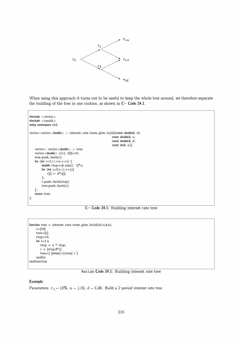
r0 �����*
HHHHHj
ru
rd
�����*
HHHHHj
���
��*
HHHHHj
ruu
rud
rdd
When using this approach it turns out to be useful to keep the whole tree around, we therefore separatethe building of the tree in one routine, as shown in C++ Code 24.1.
#include <vector>#include <cmath>using namespace std;
vector<vector<double> > interest rate trees gbm build(const double& r0,const double& u,const double& d,const int& n){
vector< vector<double> > tree;vector<double> r(1); r[0]=r0;tree.push back(r);for (int i=1;i<=n;++i) {
double rtop=r[r.size()�1]*u;for (int j=0;j<i;++j){
r[j] = d*r[j];};r.push back(rtop);tree.push back(r);
};return tree;
};
C++ Code 24.1: Building interest rate tree
function tree = interest rate trees gbm build(r0,u,d,n)r=[r0];tree=[r];rtop=r0;for i=1:n
rtop = u * rtop;r = [rtop;d*r];tree=[ [zeros(1,i);tree] r ];
endforendfunction
Matlab Code 24.1: Building interest rate tree
Example
Parameters: r0 � 10%, u = 1:02, d = 0:99. Build a 2 period interest rate tree.
215

C++ program:
vector< vector<double> > tree = interest rate trees gbm build(0.1,1.02,0.99,3);cout << " Interest rate tree: " << endl;cout << " Time 0: " << tree[0][0] << endl;cout << " Time 1: " << tree[1][0] << " " << tree[1][1] << endl;cout << " Time 2: " << tree[2][0] << " " << tree[2][1] << " " << tree[2][2] << endl;
Output from C++ program:
Interest rate tree:Time 0: 0.1Time 1: 0.099 0.102Time 2: 0.09801 0.10098 0.10404
24.2 Discount factors
We want to price bonds and other fixed income securities, which contains sets of future cash flows.Instead of interest rates we need prices, not interest rates, i.e. discount factors. The interest rate treetherefore needs to be used to generate discount factors, which needs to be specified at every point of thetree, and for all relevant maturities. Let d(t; T ) be the discount factor at time t for a time T payment.If we at time 0 want to price cash flows at time 2, we need the following set of discount factors
d(0; 2)�����
���*
HHHHHH
HHj
du(1; 2)
dd(1; 2)
In constructing trees of discount we need one additional piece of information, q, which are used as follows:
d(0; 2) = e�r0 (qdu(1; 2) + (1 + q)dd(1; 2))
The parameter q serves the same purpose as the state price probability, but it is found differently.
Exercise 24.1.
Given the prices of two discount bonds, with maturities 1 and 2, how would you back out q?
Exercise 24.2.
Suppose you have q and the tree of short interest rates. How would you calculate the t-period spot rate?
24.3 Pricing bonds
Pricing straight bonds is then just a matter of the usual recursive valuation
Example
Parameters: r0 � 10%, u = 1:02, d = 0:99. Let q = 0:5. Determine the price of a 3 period coupon bondwith coupon of 10 and face value of 100.
216
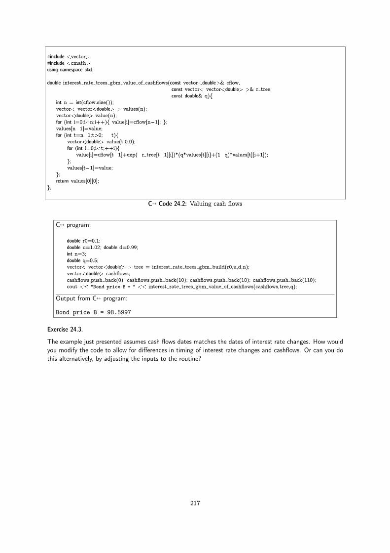
#include <vector>#include <cmath>using namespace std;
double interest rate trees gbm value of cashflows(const vector<double>& cflow,const vector< vector<double> >& r tree,const double& q){
int n = int(cflow.size());vector< vector<double> > values(n);vector<double> value(n);for (int i=0;i<n;i++){ value[i]=cflow[n�1]; };values[n�1]=value;for (int t=n�1;t>0;��t){
vector<double> value(t,0.0);for (int i=0;i<t;++i){
value[i]=cflow[t�1]+exp(�r tree[t�1][i])*(q*values[t][i]+(1�q)*values[t][i+1]);};values[t�1]=value;
};return values[0][0];
};
C++ Code 24.2: Valuing cash flows
C++ program:
double r0=0.1;double u=1.02; double d=0.99;int n=3;double q=0.5;vector< vector<double> > tree = interest rate trees gbm build(r0,u,d,n);vector<double> cashflows;cashflows.push back(0); cashflows.push back(10); cashflows.push back(10); cashflows.push back(110);cout << "Bond price B = " << interest rate trees gbm value of cashflows(cashflows,tree,q);
Output from C++ program:
Bond price B = 98.5997
Exercise 24.3.
The example just presented assumes cash flows dates matches the dates of interest rate changes. How wouldyou modify the code to allow for differences in timing of interest rate changes and cashflows. Or can you dothis alternatively, by adjusting the inputs to the routine?
217

24.4 Callable bond
A slightly more involved example is a callable bond.
#include <vector>#include <cmath>using namespace std;
double interest rate trees gbm value of callable bond(const vector<double>& cflows,const vector< vector<double> >& r tree,const double& q,const int& first call time,const double& call price){
int n = int(cflows.size());vector< vector<double> > values(n);vector<double> value(n);for (int i=0;i<n;i++){ value[i]=cflows[n�1]; };values[n�1]=value;for (int t=n�1;t>0;��t){
vector<double> value(t,0.0);for (int i=0;i<t;++i){
value[i]=cflows[t�1]+exp(�r tree[t�1][i])*(q*values[t][i]+(1�q)*values[t][i+1]);if (t>=first call time){ value[i]=min(value[i],call price); };
};values[t�1]=value;
};return values[0][0];
};
C++ Code 24.3: Valuing callable bond
Example
Construct a short rate lattice for periods (years) 0 through 9 with an initial rate of r0 = 6% and with successiverates determined by a multiplicative factors u = 1:2 or d = 0:9. Assign q = 0:5.
1. Using this lattice, find the value of a 10-year 6% bond.
2. Suppose this bond can be called by the issuing party at any time after 5 years. (When the bond iscalled, the face value plus the currently due coupon are paid at that time and the bond is canceled.)What is the fair value of this bond?
The interest rate lattice:step: 0 1 2 3 4 5 6 7 8 9nodes: 31.0
25.8 23.221.5 19.3 17.4
17.9 16.1 14.5 13.114.9 13.4 12.1 10.9 9.8
12.4 11.2 10.1 9.1 8.2 7.310.4 9.3 8.4 7.6 6.8 6.1 5.5
8.6 7.8 7.0 6.3 5.7 5.1 4.6 4.17.2 6.5 5.8 5.2 4.7 4.3 3.8 3.4 3.1
6.0 5.4 4.9 4.4 3.9 3.5 3.2 2.9 2.6 2.3
1. Valuing the noncallable bond
The cash flow lattice
218
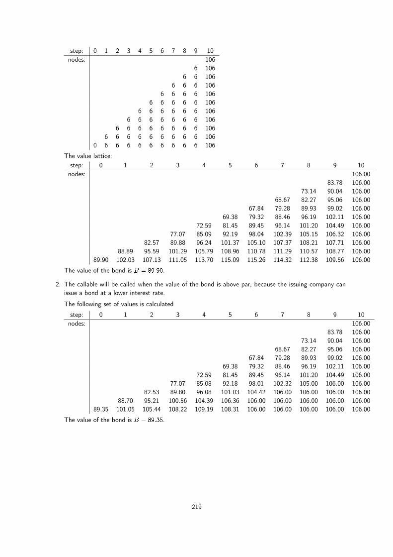
step: 0 1 2 3 4 5 6 7 8 9 10nodes: 106
6 1066 6 106
6 6 6 1066 6 6 6 106
6 6 6 6 6 1066 6 6 6 6 6 106
6 6 6 6 6 6 6 1066 6 6 6 6 6 6 6 106
6 6 6 6 6 6 6 6 6 1060 6 6 6 6 6 6 6 6 6 106
The value lattice:step: 0 1 2 3 4 5 6 7 8 9 10nodes: 106.00
83.78 106.0073.14 90.04 106.00
68.67 82.27 95.06 106.0067.84 79.28 89.93 99.02 106.00
69.38 79.32 88.46 96.19 102.11 106.0072.59 81.45 89.45 96.14 101.20 104.49 106.00
77.07 85.09 92.19 98.04 102.39 105.15 106.32 106.0082.57 89.88 96.24 101.37 105.10 107.37 108.21 107.71 106.00
88.89 95.59 101.29 105.79 108.96 110.78 111.29 110.57 108.77 106.0089.90 102.03 107.13 111.05 113.70 115.09 115.26 114.32 112.38 109.56 106.00
The value of the bond is B = 89:90.
2. The callable will be called when the value of the bond is above par, because the issuing company canissue a bond at a lower interest rate.
The following set of values is calculated
step: 0 1 2 3 4 5 6 7 8 9 10nodes: 106.00
83.78 106.0073.14 90.04 106.00
68.67 82.27 95.06 106.0067.84 79.28 89.93 99.02 106.00
69.38 79.32 88.46 96.19 102.11 106.0072.59 81.45 89.45 96.14 101.20 104.49 106.00
77.07 85.08 92.18 98.01 102.32 105.00 106.00 106.0082.53 89.80 96.08 101.03 104.42 106.00 106.00 106.00 106.00
88.70 95.21 100.56 104.39 106.36 106.00 106.00 106.00 106.00 106.0089.35 101.05 105.44 108.22 109.19 108.31 106.00 106.00 106.00 106.00 106.00
The value of the bond is B = 89:35.
219

C++ program:
double r0=0.06;double u=1.2; double d=0.9;int n=10;double q=0.5;vector< vector<double> > tree = interest rate trees gbm build(r0,u,d,n);vector<double> cashflows;cashflows.push back(0);for (int t=1;t<=9;++t){ cashflows.push back(6); };cashflows.push back(106);cout << "Straight bond price = " << interest rate trees gbm value of cashflows(cashflows,tree,q) << endl;int first call time = 6;double call price = 106;cout << "Callable bond price = "
<< interest rate trees gbm value of callable bond(cashflows,tree,q, first call time, call price) << endl;
Output from C++ program:
Straight bond price = 89.9017Callable bond price = 89.2483
Exercise 24.4.
How would you price a call option on a coupon bond in this setting?
24.5 Readings
General references include Sundaresan (2001).
Rendleman and Bartter (1979) and Rendleman and Bartter (1980) are the original references for buildingstandard binomial interest rate trees.
220

Chapter 25
Building term structure trees using the Hoand Lee (1986) approach
25.1 Intro
In this section we build interest rate trees following the orgiginal paper of Ho and Lee (1986). We willfollow the analysis in the paper, and use it to illustrate how yu can build trees of more complex termstructures than the simple binomial trees of the interest rate. The selling point of the original paper wasthat one could fit an initial term structure and then specify an evolution of the term structure consistentwith this initial term structure.
25.2 Building trees of term structures
25.3 Ho Lee term structure class
221

#include "fin_recipes.h"
class term structure class ho lee : public term structure class {private:
term structure class* initial term ;int n ;int i ;double delta ;double pi ;
public:term structure class ho lee(term structure class* fitted term,
const int & n,const int & i,const double& lambda,const double& pi);
double d(const double& T) const;};
vector< vector<term structure class ho lee> >
term structure ho lee build term structure tree(term structure class* initial,const int& no steps,const double& delta,const double& pi);
double price european call option on bond using ho lee(term structure class* initial,const double& delta,const double& pi,const vector<double>& underlying bond cflow times,const vector<double>& underlying bond cflows,const double& K,const double& option time to maturity);
Header file 25.1: Term structure class for Ho-Lee
#include "fin_recipes.h"
term structure class ho lee::term structure class ho lee(term structure class* fitted term,const int & n,const int & i,const double& delta,const double& pi){
initial term =fitted term;n =n;i =i;delta =delta;pi =pi;
};
C++ Code 25.1: Term structure class for Ho-Lee
222

#include "fin_recipes.h"//#include “term structure class ho lee.h”
inline double hT(const double& T, const double& delta, const double& pi){return (1.0/(pi+(1�pi)*pow(delta,T)));
};
double term structure class ho lee::d(const double& T) const{double d=(*initial term ).d(T+n )/(*initial term ).d(n );for (int j=1;j<n ;++j){
d *= hT(T+(n �j),delta ,pi ) / hT(n �j,delta ,pi ) ;};d *= hT(T,delta ,pi )*pow(delta ,T*(n �i ));return d;
};
C++ Code 25.2: Term structure class for Ho-Lee, calculation of discount function
#include "fin_recipes.h"
vector< vector<term structure class ho lee> >
term structure ho lee build term structure tree(term structure class* initial,const int& no steps,const double& delta,const double& pi){
vector< vector<term structure class ho lee> > hl tree;for (int t=0;t<5;++t){
hl tree.push back(vector<term structure class ho lee>());for (int j=0;j<=t;++j){
term structure class ho lee hl(initial,t,j,delta,pi);hl tree[t].push back(hl);
};};return hl tree;
};
C++ Code 25.3: Building a term structure tree
223

25.4 Pricing things
We now have access to what we need to do pricing through the recursive relationship
C(n; i) = [�C(n+ 1; i+ 1) + (1� �)C(n+ i; i)]P(n)i (1)
where C(n; i) is the value of a security at time n at node i.
What we are pricing are typically state and time-contingent claims to cash flows. Let us illustrate pricingof an (European) call option on some underlying bond. Suppose this bond is risk free. Its cash flowsat each future date does not depend on the state, but the timing of cash flows changes as you movein the tree. It is therefore necessary to some way figure out at date t: What are the future cash flowswhen you want to price the underlying bond at that date. We build a small class that contains thisinformation, and use it, together with the term structures in the individual nodes, to find the bond priceat each node. The value of the bond at the different nodes change because the term structure you usefor discounting is changing. This bond price is then used to find the option value at each node.
224

#include "fin_recipes.h"
class time contingent cash flows{public:
vector<double> times;vector<double> cash flows;time contingent cash flows(const vector<double>& in times, const vector<double>& in cflows){
times=in times; cash flows=in cflows;};int no cflows(){ return int(times.size()); };
};
vector<time contingent cash flows>build time series of bond time contingent cash flows(const vector<double>& initial times,
const vector<double>& initial cflows){vector<time contingent cash flows> vec cf;vector<double> times = initial times;vector<double> cflows = initial cflows;while (times.size()>0){
vec cf.push back(time contingent cash flows(times,cflows));vector<double> tmp times;vector<double> tmp cflows;for (int i=0;i<times.size();++i){
if (times[i]�1.0>=0.0) {tmp times.push back(times[i]�1);tmp cflows.push back(cflows[i]);
};};times = tmp times; cflows = tmp cflows;
};return vec cf;
};
double price european call option on bond using ho lee(term structure class* initial, const double& delta, const double& pi,const vector<double>& underlying bond cflow times,const vector<double>& underlying bond cflows,const double& K, const double& time to maturity){
int T = int(time to maturity+0.0001);vector<vector<term structure class ho lee> > hl tree
= term structure ho lee build term structure tree(initial,T+1,delta,pi);vector<time contingent cash flows> vec cf
= build time series of bond time contingent cash flows(underlying bond cflow times, underlying bond cflows);
vector<double> values(T+1);for (int i=0;i<=T;++i){
values[i]=max(0.0,bonds price(vec cf[T+1].times, vec cf[T+1].cash flows, hl tree[T+1][i]) � K);};for (int t=T;t>=0;��t){
vector<double> values this(t+1);for (int i=0;i<=t;++i){ values this[i]=(pi*values[i+1]+(1.0�pi)*values[i])*hl tree[t][i].d(1); };values=values this;
};return values[0];
};
C++ Code 25.4: Pricing of European call option on straight bond using Ho-Lee
225

Example
You are pricing options on a 5 year zero coupon risk free bond. The options are European calls with a timeto maturity of 3 years.
You will price the options using a Ho-Lee approach with parameters � = 0:5 and � = 0:98.
Price the option using two different assumptions about the current term structure:
1. The term structure is flat with an interest rate of 10% (continously compounded).
2. The current term structure has been estimated using a Nelson Siegel parameterization with parameters�0 = 0:09, �1 = 0:01, �2 = 0:01 and � = 5:0.
C++ program:
double delta=0.98;double pi=0.5;double r=0.1;term structure class* initial=new term structure class flat(r);vector<double> times; times.push back(5.0);vector<double> cflows; cflows.push back(100);double K=80;double time to maturity=3;cout << " Flat term structure " << endl;cout << " c= " << price european call option on bond using ho lee(initial,delta, pi, times,cflows,K,time to maturity);cout << endl;delete (initial);double beta0=0.09; double beta1=0.01; double beta2=0.01; double lambda=5.0;initial = new term structure class nelson siegel(beta0,beta1,beta2,lambda);cout << " Nelson Siegel term structure " << endl;cout << " c= " << price european call option on bond using ho lee(initial,delta, pi, times,cflows,K,time to maturity);cout << endl;
Output from C++ program:
Flat term structurec= 6.46323Nelson Siegel term structurec= 6.33238
Exercise 25.1.
What changes do you need to make to C++ Code 25.4 to price an American call option instead of an Europeancall?
Exercise 25.2.
If you for example want to price a bond, you need to keep track of intermediate payments of coupon.Implement such a procedure. To see that it is correct us it to price a (straight) bond and then compare thevalue calculated in the tree with the value using the current term structure. Then modify the code to buildin a callable bond feature. What additional informaiton must be kept track of?
Exercise 25.3.
In the Ho and Lee (1986) paper there is a typo in equation (22). Can you see what it is?
25.5 References
The discussion in this chapter follows closely the original paper Ho and Lee (1986)
226
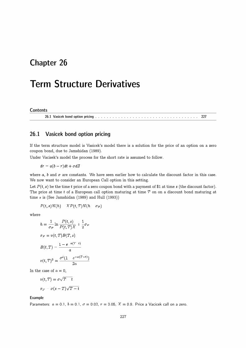
Chapter 26
Term Structure Derivatives
Contents26.1 Vasicek bond option pricing . . . . . . . . . . . . . . . . . . . . . . . . . . . . . . . . . . . . 227
26.1 Vasicek bond option pricing
If the term structure model is Vasicek’s model there is a solution for the price of an option on a zerocoupon bond, due to Jamshidan (1989).
Under Vacisek’s model the process for the short rate is assumed to follow.
dr = a(b� r)dt+ �dZ
where a, b and � are constants. We have seen earlier how to calculate the discount factor in this case.We now want to consider an European Call option in this setting.
Let P (t; s) be the time t price of a zero coupon bond with a payment of $1 at time s (the discount factor).The price at time t of a European call option maturing at time T on on a discount bond maturing attime s is (See Jamshidan (1989) and Hull (1993))
P (t; s)N(h)�XP (t; T )N(h� �P )
where
h =1
�Pln
P (t; s)
P (t; T )X+
1
2�P
�P = v(t; T )B(T; s)
B(t; T ) =1� e�a(T�t)
a
v(t; T )2 =�2(1� e�a(T�t))
2a
In the case of a = 0,
v(t; T ) = �pT � t
�P = �(s� T )pT � t
Example
Parameters: a = 0:1, b = 0:1, � = 0:02, r = 0:05, X = 0:9. Price a Vacicek call on a zero.
227

#include "normdist.h"#include "fin_recipes.h"#include <cmath>using namespace std;
double bond option price call zero vasicek(const double& X, // exercise priceconst double& r, // current interest rateconst double& option time to maturity,const double& bond time to maturity,const double& a, // parametersconst double& b,const double& sigma){
double T t = option time to maturity;double s t = bond time to maturity;double T s = s t�T t;double v t T;double sigma P;if (a==0.0) {
v t T = sigma * sqrt ( T t ) ;sigma P = sigma*T s*sqrt(T t);
}else {
v t T = sqrt (sigma*sigma*(1�exp(�2*a*T t))/(2*a));double B T s = (1�exp(�a*T s))/a;sigma P = v t T*B T s;
};double h = (1.0/sigma P) * log (term structure discount factor vasicek(s t,r,a,b,sigma)/
(term structure discount factor vasicek(T t,r,a,b,sigma)*X) )+ sigma P/2.0;
double c = term structure discount factor vasicek(s t,r,a,b,sigma)*N(h)�X*term structure discount factor vasicek(T t,r,a,b,sigma)*N(h�sigma P);
return c;};
C++ Code 26.1: Bond option pricing using the Vasicek model
C++ program:
double a = 0.1; double b = 0.1; double sigma = 0.02; double r = 0.05; double X=0.9;cout << " Vasicek call option price "
<< bond option price call zero vasicek(X,r,1,5,a,b,sigma) << endl;
Output from C++ program:
Vasicek call option price 0.000226833
228
Chapter 27
Date (and time) revisited - the BOOSTlibraries
In the introduction we used the construction of a date class as an example of building a nontrivial (anduseful) class. However, even if we follow the hints in the exercises, and use the operating system utilitiesfor dealing with dates, at some point such a “homespun” date class needs to be replaced with somethingmore reliable.
The date class that is most likely to spring to the programmers’ minds these days is one provided bythe Boost C++ library. Let us therefore use this opportunity to introduce the Boost libraries, and showsome examples of date usage. The Boost libraries are collections of C++ libraries, many of which may atsome point become part of the C++ standard.1 One of the most useful of the Boost libraries are completelibraries for date (gregorian) and date and time (date_time.
We are not going to go into detail here, we limit ourselves to showing some examples of usage:1Ten Boost libraries actually became part of the latest C++ standard (C++-11). If you have a recent C++ implementation,
the Boost libraries are typically included.
229

C++ program:
#include "boost/date_time/gregorian/gregorian.hpp"#include "boost/date_time/posix_time/posix_time.hpp"#include <iostream>using namespace std;using namespace boost::gregorian;using namespace boost::posix time;
void ex date time(){boost::gregorian::date d(2014,4,1); // creating a datecout << " date: " << d << endl;
boost::posix time::ptime dt;stringstream ss("2014-mar-01 10:01:01.01");ss >> dt;cout << " date time just created: " << dt << endl;
ptime now = second clock::local time(); //get the current time from the clockdate today = now.date(); //Get the date part out of the timecout << " today: " << today << endl;date tommorrow = today + days(1); // add one dateptime tommorrow start(tommorrow); //midnighttime duration remaining = tommorrow start � now;std::cout << "Time left till midnight: " << to simple string(remaining) << std::endl;
}
Output from C++ program:
date: 2014-Apr-01date time just created: 2014-Mar-01 10:01:01.010000today: 2014-Jun-30Time left till midnight: 10:19:33
27.1 References
The Boost homepage is at http://www.boost.org/
230
Appendix A
Normal Distribution approximations.
ContentsA.1 The normal distribution function . . . . . . . . . . . . . . . . . . . . . . . . . . . . . . . . . 231A.2 The cumulative normal distribution . . . . . . . . . . . . . . . . . . . . . . . . . . . . . . . . 232A.3 Multivariate normal . . . . . . . . . . . . . . . . . . . . . . . . . . . . . . . . . . . . . . . . 232A.4 Calculating cumulative bivariate normal probabilities . . . . . . . . . . . . . . . . . . . . . . . 233A.5 Simulating random normal numbers . . . . . . . . . . . . . . . . . . . . . . . . . . . . . . . . 235A.6 Cumulative probabilities for general multivariate distributions . . . . . . . . . . . . . . . . . . . 236A.7 Implementation in C++11 . . . . . . . . . . . . . . . . . . . . . . . . . . . . . . . . . . . . . 236A.8 References . . . . . . . . . . . . . . . . . . . . . . . . . . . . . . . . . . . . . . . . . . . . 236
We will in general not go into detail about more standard numerical problems not connected to finance,there are a number of well known sources for such, but we show the example of calculations involvingthe normal distribution.
A.1 The normal distribution function
The nurmal distribution function
n(x) = e�x2
2
is calculated as
#include <cmath> // c library of math functionsusing namespace std; // which is part of the standard namespace
// most C compilers define PI, but just in case it doesn’t#ifndef PI#define PI 3.141592653589793238462643#endif
double n(const double& z) { // normal distribution functionreturn (1.0/sqrt(2.0*PI))*exp(�0.5*z*z);
};
C++ Code A.1: The normal distribution function
231

A.2 The cumulative normal distribution
The solution of a large number of option pricing formulas are written in terms of the cumulative normaldistribution. For a random variable x the cumulative probability is the probability that the outcomeis lower than a given value z. To calculate the probability that a normally distubuted random variablewith mean 0 and unit variance is less than z, N(z), one have to evaluate the integral
Prob(x � z) = N(z) =
Z z
�1n(x)dx =
Z z
�1e�
x2
2 dx
There is no explicit closed form solution for calculation of this integral, but a large number of well knownapproximations exists. Abramowiz and Stegun (1964) is a good source for these approximations. Thefollowing is probably the most used such approximation, it being pretty accurate and relatively fast.The arguments to the function are assumed normalized to a (0,1) distribution.
#include <cmath> // math functions.using namespace std;
double N(const double& z) {if (z > 6.0) { return 1.0; }; // this guards against overflowif (z < �6.0) { return 0.0; };
double b1 = 0.31938153;double b2 = �0.356563782;double b3 = 1.781477937;double b4 = �1.821255978;double b5 = 1.330274429;double p = 0.2316419;double c2 = 0.3989423;
double a=fabs(z);double t = 1.0/(1.0+a*p);double b = c2*exp((�z)*(z/2.0));double n = ((((b5*t+b4)*t+b3)*t+b2)*t+b1)*t;n = 1.0�b*n;if ( z < 0.0 ) n = 1.0 � n;return n;
};
C++ Code A.2: The cumulative normal
A.3 Multivariate normal
The normal distribution is also defined for several random variables. We then characterise the vector ofrandom variables
X =
26664x1x2...xn
37775A probability statement about this vector is a joint statement about all elements of the vector.
232
A.4 Calculating cumulative bivariate normal probabilities
The most used multivariate normal calculation is the bivariate case, where we let x and y be bivariatenormally distributed, each with mean 0 and variance 1, and assume the two variables have correlationof �. By the definition of correlation � 2 [�1; 1]. The cumulative probability distribution
P (x < a; y < b) = N(a; b; �)
=
Z a
�1
Z b
�1
1
2�p1� �2
exp
��1
2
x2 � 2�xy + y2
1� �2
�dxdy
There are several approximations to this integral. We pick one such, discussed in (Hull, 1993, Ch 10),shown in C++ Code A.3.
If one has more than two correlated variables, the calculation of cumulative probabilites is a nontrivialproblem. One common method involves Monte Carlo estimation of the definite integral. We will considerthis, but then it is necessary to first consider simulation of random normal variables.
Example
Calculate N(0) and N(0,0,0)
C++ program:
cout << " N(0) = " << N(0) << endl;cout << " N(0,0,0) = " << N(0,0,0) << endl;
Output from C++ program:
N(0) = 0.5N(0,0,0) = 0.25
233
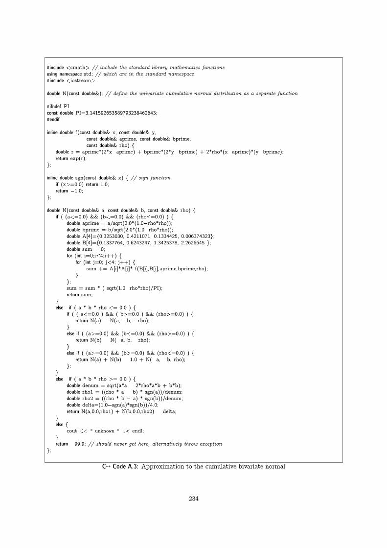
#include <cmath> // include the standard library mathematics functionsusing namespace std; // which are in the standard namespace#include <iostream>
double N(const double&); // define the univariate cumulative normal distribution as a separate function
#ifndef PIconst double PI=3.141592653589793238462643;#endif
inline double f(const double& x, const double& y,const double& aprime, const double& bprime,const double& rho) {
double r = aprime*(2*x�aprime) + bprime*(2*y�bprime) + 2*rho*(x�aprime)*(y�bprime);return exp(r);
};
inline double sgn(const double& x) { // sign functionif (x>=0.0) return 1.0;return �1.0;
};
double N(const double& a, const double& b, const double& rho) {if ( (a<=0.0) && (b<=0.0) && (rho<=0.0) ) {
double aprime = a/sqrt(2.0*(1.0�rho*rho));double bprime = b/sqrt(2.0*(1.0�rho*rho));double A[4]={0.3253030, 0.4211071, 0.1334425, 0.006374323};double B[4]={0.1337764, 0.6243247, 1.3425378, 2.2626645 };double sum = 0;for (int i=0;i<4;i++) {
for (int j=0; j<4; j++) {sum += A[i]*A[j]* f(B[i],B[j],aprime,bprime,rho);
};};sum = sum * ( sqrt(1.0�rho*rho)/PI);return sum;
}else if ( a * b * rho <= 0.0 ) {
if ( ( a<=0.0 ) && ( b>=0.0 ) && (rho>=0.0) ) {return N(a) � N(a, �b, �rho);
}else if ( (a>=0.0) && (b<=0.0) && (rho>=0.0) ) {
return N(b) � N(�a, b, �rho);}else if ( (a>=0.0) && (b>=0.0) && (rho<=0.0) ) {
return N(a) + N(b) � 1.0 + N(�a, �b, rho);};
}else if ( a * b * rho >= 0.0 ) {
double denum = sqrt(a*a � 2*rho*a*b + b*b);double rho1 = ((rho * a � b) * sgn(a))/denum;double rho2 = ((rho * b � a) * sgn(b))/denum;double delta=(1.0�sgn(a)*sgn(b))/4.0;return N(a,0.0,rho1) + N(b,0.0,rho2) � delta;
}else {
cout << " unknown " << endl;}return �99.9; // should never get here, alternatively throw exception
};
C++ Code A.3: Approximation to the cumulative bivariate normal
234

A.5 Simulating random normal numbers
Generation of random numbers is a large topic and is treated at length in such sources as Knuth(1997). The generated numbers can never be truly random, only “pseudo”-random, they will be generatedaccording to some reproducible algorithm and after a (large) number of random number generations thesequence will start repeating itself. The number of iterations before replication starts is a measure of thequality of a random number generator. For anybody requiring high-quality random number generatorsthe rand() function provided by the standard C++ library should be avoided, but for not getting intoinvolved discussion of random number generations we use this function as a basis for the generation ofuniformly distributed numbers in the interval [0; 1), as shown in C++ Code A.4.
#include <cstdlib>using namespace std;
double random uniform 0 1(void){return double(rand())/double(RAND MAX); // this uses the C library random number generator.
};
C++ Code A.4: Pseudorandom numbers from an uniform [0; 1) distribution
Exercise A.1.
Replace the random_uniform function here by an alternative of higher quality, by looking into what numericallibraries is available on your computing platform, or by downloading a high quality random number generatorfrom such places as mathlib or statlib.
These uniformly distributed distributed random variates are used as a basis for the polar method fornormal densities discussed in Knuth (1997) and inplemented as shown in C++ Code A.5.
#include <cmath>#include <cstdlib>using namespace std;
double random uniform 0 1(void);
double random normal(void){double U1, U2, V1, V2;double S=2;while (S>=1) {
U1 = random uniform 0 1();U2 = random uniform 0 1();V1 = 2.0*U1�1.0;V2 = 2.0*U2�1.0;S = pow(V1,2)+pow(V2,2);
};double X1=V1*sqrt((�2.0*log(S))/S);return X1;
};
C++ Code A.5: Pseudorandom numbers from a normal (0; 1) distribution
Example
1. Generate 5 random uniform numbers (0,1)
2. Generate 5 random N(0,1) numbers.
235

C++ program:
cout << " 5 random uniform numbers between 0 and 1: " << endl;cout << " ";for (int i=0;i<5;++i){ cout << " " << random uniform 0 1(); }; cout << endl;cout << " 5 random normal(0,1) numbers: " << endl;cout << " ";for (int i=0;i<5;++i){ cout << " " << random normal() ; }; cout << endl;
Output from C++ program:
5 random uniform numbers between 0 and 1:0.840188 0.394383 0.783099 0.79844 0.911647
5 random normal(0,1) numbers:-1.07224 0.925946 2.70202 1.36918 0.0187313
A.6 Cumulative probabilities for general multivariate distributions
When moving beyond the bivariate case calculation of probability integrals become more of an exercisein general numerical integration. A typical tool is Monte Carlo integration, but that is not the onlypossibility.
A.7 Implementation in C++11
The latest standard of the C++ language, C++11, includes a library for generating random numbers. See(Stroustrup, 1997a, Section 5.6.3).
A.8 References
Tong (1990) discusses the multivariate normal distribution, and is a good reference. For the ultimatesource, see Knuth (1997).
236
Appendix B
C++ concepts
This chapter contains a listing of various C/C++ concepts and some notes on each of them.
accumulate() Function accumulating the elements of a sequence.
bool Boolean variable, taking on the two values true and false. For historical reasons one can alsouse the values zero and one for false and true.
class (C++ keyword).
const (qualifyer to variable in C++ function call).
double (basic type). A floating point number with high accuracy.
exp(x) (C function). Defined in <cmath>. Returns the natural exponent e to the given power x, ex.
fabs
float (basic type). A floating point number with limited accuracy.
for Loop
header file
if
Indexation (in vectors and matrices). To access element number i in an array A, use A[i-1]. Wellknown trap for people coming to C from other languages. Present in C for historical efficiencyreasons. Arrays in C were implemented using pointers. Indexing was done by finding the firstelement of the array, and then adding pointers to find the indexed element. The first element is ofcourse found by adding nothing to the first elment, hence the first element was indexed by zero.
include
inline (qualifyer to C++ function name). Hint to the optimizer that this function is most efficientlyimplemented by inlining it, or putting the full code of the function into each instance of itscalling. Has the side effect of making the function local to the file in which it is defined.
int (basic type). An integer with a limited number of significant digits.
log(x) (C function). Defined in <cmath>. Calculates the natural logarithm ln(x) of its argument.
long (basic type). An integer that can contain a large number.
min_element() (C++ function)
237

max_element (C++ function)
namespace (C++ concept)
return
standard namespace (C++ concept)
string (C++ basic type)
using (C++ concept)
vector (C++ container class). Defined in <vector>
while
238

Appendix C
Interfacing to external libraries
ContentsC.1 Boost . . . . . . . . . . . . . . . . . . . . . . . . . . . . . . . . . . . . . . . . . . . . . . . 239C.2 Newmat . . . . . . . . . . . . . . . . . . . . . . . . . . . . . . . . . . . . . . . . . . . . . . 239C.3 IT++ . . . . . . . . . . . . . . . . . . . . . . . . . . . . . . . . . . . . . . . . . . . . . . . 239C.4 GSL . . . . . . . . . . . . . . . . . . . . . . . . . . . . . . . . . . . . . . . . . . . . . . . . 239
C.4.1 The evaluation of N3 . . . . . . . . . . . . . . . . . . . . . . . . . . . . . . . . . 239C.5 Internet links . . . . . . . . . . . . . . . . . . . . . . . . . . . . . . . . . . . . . . . . . . . 240
In various places we have used routines from other public domain packages. In this appendix there aresome notes about the libraries which are referenced, and some comments about linking to them.
C.1 Boost
Large collection of peer-reviewed code. Particularly useful: the date_time library.
C.2 Newmat
Newmat is a matrix library that attempts to do matlab-like operations in C++, in that one can definematrices and vectors, and then multiply them and so on without needing to explicitly call subroutines,instead writing the operations in a more mathematically oriented way.
C.3 IT++
IT++ is a large library with various different
C.4 GSL
C.4.1 The evaluation of N3
In the calculation of the American Put approximation of Geske and Johnson (1984), a trivariate normalneeds to be evaluated. Following the discussion in the paper, this is evaluated as
N3(h; k; j; �12; �13; �23) =
Z j
�1n(z)N2
k � �23zp1� �223
;h� �13zp1� �213
;�12 � �13�23p1� �213
p1� �223
!
239
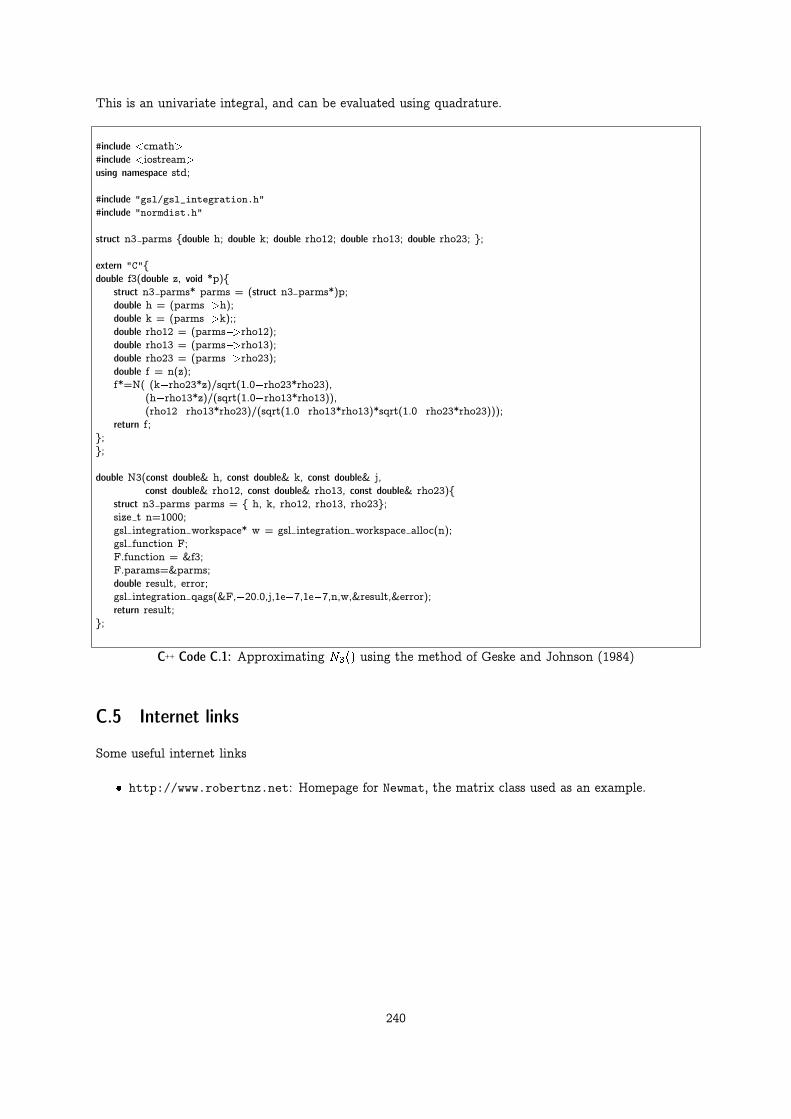
This is an univariate integral, and can be evaluated using quadrature.
#include <cmath>#include <iostream>using namespace std;
#include "gsl/gsl_integration.h"#include "normdist.h"
struct n3 parms {double h; double k; double rho12; double rho13; double rho23; };
extern "C"{double f3(double z, void *p){
struct n3 parms* parms = (struct n3 parms*)p;double h = (parms�>h);double k = (parms�>k);;double rho12 = (parms�>rho12);double rho13 = (parms�>rho13);double rho23 = (parms�>rho23);double f = n(z);f*=N( (k�rho23*z)/sqrt(1.0�rho23*rho23),
(h�rho13*z)/(sqrt(1.0�rho13*rho13)),(rho12�rho13*rho23)/(sqrt(1.0�rho13*rho13)*sqrt(1.0�rho23*rho23)));
return f;};};
double N3(const double& h, const double& k, const double& j,const double& rho12, const double& rho13, const double& rho23){
struct n3 parms parms = { h, k, rho12, rho13, rho23};size t n=1000;gsl integration workspace* w = gsl integration workspace alloc(n);gsl function F;F.function = &f3;F.params=&parms;double result, error;gsl integration qags(&F,�20.0,j,1e�7,1e�7,n,w,&result,&error);return result;
};
C++ Code C.1: Approximating N3() using the method of Geske and Johnson (1984)
C.5 Internet links
Some useful internet links
� http://www.robertnz.net: Homepage for Newmat, the matrix class used as an example.
240

Appendix D
Summarizing routine names
In many of the algorithms use is made of other routines. To simplify the matter all routines are summarised in one header file,fin_recipes.h. This appendix shows this file.
// file: fin recipes.h// author: Bernt Arne Oedegaard// defines all routines in the financial numerical recipes “book”
#ifndef FIN RECIPES H#define FIN RECIPES H
#include <vector>#include <cmath>using namespace std;
///////// present value ////////////////////////////////////// discrete coumpounding/////////////////////////////////// discrete, annual compounding
double cash flow pv discrete ( const vector<double>& cflow times, const vector<double>& cflow amounts,const double& r);
double cash flow irr discrete(const vector<double>& cflow times, const vector<double>& cflow amounts);bool cash flow unique irr(const vector<double>& cflow times, const vector<double>& cflow amounts);double bonds price discrete(const vector<double>& cashflow times, const vector<double>& cashflows,
const double& r);double bonds yield to maturity discrete(const vector<double>& times,
const vector<double>& amounts,const double& bondprice);
double bonds duration discrete(const vector<double>& times,const vector<double>& cashflows,const double& r);
double bonds duration macaulay discrete(const vector<double>& cashflow times,const vector<double>& cashflows,const double& bond price);
double bonds duration modified discrete (const vector<double>& times,const vector<double>& amounts,const double& bond price);
double bonds convexity discrete(const vector<double>& cflow times,const vector<double>& cflow amounts,const double& r);
/////////////////////////////////// continous compounding.double cash flow pv(const vector<double>& cflow times,const vector<double>& cflow amounts,const double& r);double cash flow irr(const vector<double>& cflow times, const vector<double>& cflow amounts);double bonds price(const vector<double>& cashflow times, const vector<double>& cashflows, const double& r);double bonds price(const vector<double>& coupon times, const vector<double>& coupon amounts,
const vector<double>& principal times, const vector<double>& principal amounts,const double& r);
241

double bonds duration(const vector<double>& cashflow times, const vector<double>& cashflows,const double& r);
double bonds yield to maturity(const vector<double>& cashflow times,const vector<double>& cashflow amounts,const double& bondprice);
double bonds duration macaulay(const vector<double>& cashflow times, const vector<double>& cashflows,const double& bond price);
double bonds convexity(const vector<double>& cashflow times, const vector<double>& cashflow amounts,const double& y );
/// term structure basics
double term structure yield from discount factor(const double& dfact, const double& t);double term structure discount factor from yield(const double& r, const double& t);double term structure forward rate from discount factors(const double& d t1, const double& d t2,
const double& time);double term structure forward rate from yields(const double& r t1, const double& r t2,
const double& t1, const double& t2);double term structure yield linearly interpolated(const double& time,
const vector<double>& obs times,const vector<double>& obs yields);
// a term structure class
class term structure class {public:
virtual ˜term structure class();virtual double r(const double& t) const; // short rate, yield on zero coupon bondvirtual double d(const double& t) const; // discount factorvirtual double f(const double& t1, const double& t2) const; // forward rate
};
class term structure class flat : public term structure class {private:
double R ; // interest ratepublic:
term structure class flat(const double& r);virtual ˜term structure class flat();virtual double r(const double& t) const;void set int rate(const double& r);
};
class term structure class interpolated : public term structure class {private:
vector<double> times ; // use to keep a list of yieldsvector<double> yields ;void clear();
public:term structure class interpolated();term structure class interpolated(const vector<double>& times, const vector<double>& yields);virtual ˜term structure class interpolated();term structure class interpolated(const term structure class interpolated&);term structure class interpolated operator= (const term structure class interpolated&);
int no observations() const { return int(times .size()); };virtual double r(const double& T) const;void set interpolated observations(vector<double>& times, vector<double>& yields);
};
// using the term structure classes
double bonds price(const vector<double>& cashflow times,const vector<double>& cashflows,const term structure class& d);
double bonds duration(const vector<double>& cashflow times,const vector<double>& cashflow amounts,const term structure class& d);
242

double bonds convexity(const vector<double>& cashflow times,const vector<double>& cashflow amounts,const term structure class& d);
//// Futures pricingdouble futures price(const double& S, const double& r, const double& time to maturity);
/// Binomial option pricing
// one periode binomialdouble option price call european binomial single period( const double& S, const double& K, const double& r,
const double& u, const double& d);// multiple periode binomial
double option price call european binomial multi period given ud( const double& S, const double& K, const double& r,const double& u, const double& d, const int& no periods);
// multiple periode binomialvector< vector<double> > binomial tree(const double& S0, const double& u,const double& d,
const int& no steps);
/// Black Scholes formula //////////////////////////////////////////
double option price call black scholes(const double& S, const double& K, const double& r,const double& sigma, const double& time) ;
double option price put black scholes (const double& S, const double& K, const double& r,const double& sigma, const double& time) ;
doubleoption price implied volatility call black scholes newton( const double& S, const double& K,
const double& r, const double& time,const double& option price);
doubleoption price implied volatility put black scholes newton( const double& S, const double& K,
const double& r, const double& time,const double& option price);
double option price implied volatility call black scholes bisections( const double& S, const double& K,const double& r, const double& time,const double& option price);
double option price implied volatility put black scholes bisections( const double& S, const double& K,const double& r, const double& time,const double& option price);
double option price delta call black scholes(const double& S, const double& K, const double& r,const double& sigma, const double& time);
double option price delta put black scholes (const double& S, const double& K, const double& r,const double& sigma, const double& time);
void option price partials call black scholes(const double& S, const double& K, const double& r,const double& sigma, const double& time,double& Delta, double& Gamma, double& Theta,double& Vega, double& Rho);
void option price partials put black scholes(const double& S, const double& K, const double& r,const double& sigma, const double& time,double& Delta, double& Gamma, double& Theta,double& Vega, double& Rho);
/// warrant pricedouble warrant price adjusted black scholes(const double& S, const double& K,
const double& r, const double& sigma,const double& time,const double& no warrants outstanding,const double& no shares outstanding);
double warrant price adjusted black scholes(const double& S, const double& K,const double& r, const double& q,const double& sigma, const double& time,const double& no warrants outstanding,
243
const double& no shares outstanding);
/// Extensions of the Black Scholes model //////////////
double option price european call payout(const double& S, const double& K, const double& r,const double& b, const double& sigma, const double& time);
double option price european put payout (const double& S, const double& K, const double& r,const double& b, const double& sigma, const double& time);
double option price european call dividends(const double& S, const double& K, const double& r,const double& sigma, const double& time,const vector<double>& dividend times,const vector<double>& dividend amounts );
double option price european put dividends( const double& S, const double& K, const double& r,const double& sigma,const double& time,const vector<double>& dividend times,const vector<double>& dividend amounts);
double option price american call one dividend(const double& S, const double& K, const double& r,const double& sigma,const double& tau, const double& D1, const double& tau1);
double futures option price call european black(const double& F, const double& K, const double& r,const double& sigma, const double& time);
double futures option price put european black(const double& F, const double& K, const double& r,const double& sigma, const double& time);
double currency option price call european(const double& S, const double& K, const double& r,const double& r f, const double& sigma, const double& time);
double currency option price put european(const double& S, const double& K, const double& r,const double& r f, const double& sigma, const double& time);
double option price american perpetual call(const double& S, const double& K, const double& r,const double& q, const double& sigma);
double option price american perpetual put(const double& S, const double& K, const double& r,const double& q, const double& sigma);
// binomial option approximation ////////////////
double option price call european binomial(const double& S, const double& K, const double& r,const double& sigma, const double& t, const int& steps);
double option price put european binomial (const double& S, const double& K, const double& r,const double& sigma, const double& t, const int& steps);
double option price call american binomial(const double& S, const double& K, const double& r,const double& sigma, const double& t, const int& steps);
double option price put american binomial (const double& S, const double& K, const double& r,const double& sigma, const double& t, const int& steps);
double option price call american binomial(const double& S, const double& K,const double& r, const double& y,const double& sigma, const double& t, const int& steps);
double option price put american binomial (const double& S, const double& K, const double& r,const double& y, const double& sigma,const double& t, const int& steps);
double option price call american discrete dividends binomial( const double& S, const double& K,const double& r,const double& sigma, const double& t,const int& steps,const vector<double>& dividend times,const vector<double>& dividend amounts);
double option price put american discrete dividends binomial(const double& S, const double& K,const double& r,const double& sigma, const double& t,const int& steps,const vector<double>& dividend times,const vector<double>& dividend amounts);
double option price call american proportional dividends binomial(const double& S, const double& K,const double& r, const double& sigma,const double& time, const int& no steps,const vector<double>& dividend times,
244

const vector<double>& dividend yields);
double option price put american proportional dividends binomial( const double& S, const double& K, const double& r,const double& sigma, const double& time, const int& no steps,const vector<double>& dividend times,const vector<double>& dividend yields);
double option price delta american call binomial(const double& S, const double& K, const double& r,const double& sigma, const double& t, const int& no steps);
double option price delta american put binomial(const double& S, const double& K, const double& r,const double& sigma, const double& t, const int& no steps);
void option price partials american call binomial(const double& S, const double& K, const double& r,const double& sigma, const double& time, const int& no steps,double& delta, double& gamma, double& theta,double& vega, double& rho);
void option price partials american put binomial(const double& S, const double& K, const double& r,const double& sigma, const double& time, const int& no steps,double& delta, double& gamma, double& theta,double& vega, double& rho);
double futures option price call american binomial(const double& F, const double& K, const double& r, const double& sigma,const double& time, const int& no steps);
double futures option price put american binomial( const double& F, const double& K, const double& r, const double& sigma,const double& time, const int& no steps);
double currency option price call american binomial( const double& S, const double& K, const double& r, const double& r f,const double& sigma, const double& t, const int& n);
double currency option price put american binomial( const double& S, const double& K, const double& r, const double& r f,const double& sigma, const double& t, const int& n);
//////////////////// finite differences //////////////////
double option price call american finite diff explicit( const double& S, const double& K, const double& r,const double& sigma, const double& time,const int& no S steps, const int& no t steps);
double option price put american finite diff explicit( const double& S, const double& K, const double& r,const double& sigma, const double& time,const int& no S steps, const int& no t steps);
double option price call european finite diff explicit( const double& S, const double& K, const double& r,const double& sigma, const double& time,const int& no S steps, const int& no t steps);
double option price put european finite diff explicit( const double& S, const double& K, const double& r,const double& sigma, const double& time,const int& no S steps, const int& no t steps);
double option price call american finite diff implicit( const double& S, const double& K, const double& r,const double& sigma, const double& time,const int& no S steps, const int& no t steps);
double option price put american finite diff implicit( const double& S, const double& K, const double& r,const double& sigma, const double& time,const int& no S steps, const int& no t steps);
double option price call european finite diff implicit( const double& S, const double& K, const double& r,const double& sigma, const double& time,const int& no S steps, const int& no t steps);
double option price put european finite diff implicit( const double& S, const double& K, const double& r,const double& sigma, const double& time,const int& no S steps, const int& no t steps);
245

///////////////////////// simulated option prices //////////////////////////////////////// Payoff only function of terminal pricedouble option price call european simulated(const double& S, const double& K,
const double& r, const double& sigma,const double& time to maturity, const int& no sims);
double option price put european simulated(const double& S, const double& K,const double& r, const double& sigma,const double& time to maturity, const int& no sims);
double option price delta call european simulated(const double& S, const double& K,const double& r, const double& sigma,const double& time to maturity, const int& no sims);
double option price delta put european simulated(const double& S, const double& K,const double& r, const double& sigma,const double& time to maturity, const int& no sims);
double simulate lognormal random variable(const double& S, const double& r, const double& sigma,const double& time);
doublederivative price simulate european option generic( const double& S, const double& K,
const double& r, const double& sigma,const double& time,double payoff(const double& S, const double& K),const int& no sims);
doublederivative price simulate european option generic with control variate(const double& S, const double& K,
const double& r,const double& sigma,const double& time,double payoff(const double& S,
const double& K),const int& no sims);
doublederivative price simulate european option generic with antithetic variate(const double& S, const double& K,
const double& r,const double& sigma,const double& time,double payoff(const double& S,
const double& K),const int& no sims);
/////////////////////////////// payoffs of various options, to be used as function arguments in above simulationsdouble payoff call(const double& S, const double& K);double payoff put (const double& S, const double& K);double payoff cash or nothing call(const double& S, const double& K);double payoff asset or nothing call(const double& S, const double& K);
/////////// approximated option prices ////////////////////////double option price american put approximated johnson( const double& S, const double& X, const double& r,
const double& sigma, const double& time );
double option price american call approximated baw(const double& S, const double& K,const double& r, const double& b,const double& sigma, const double& time);
double option price american put approximated baw(const double& S, const double& K,const double& r, const double& b,const double& sigma, const double& time);
double option price american put approximated geske johnson( const double& S, const double& X,const double& r, const double& sigma,const double& time );
double option price american call approximated bjerksund stensland( const double& S,const double& X,const double& r,const double& q,const double& sigma,const double& time );
246
double option price american put approximated bjerksund stensland( const double& S,const double& X,const double& r,const double& q,const double& sigma,const double& T );
////////////// path dependent and other exotic options ////////////////////////////////
double option price call bermudan binomial(const double& S, const double& K, const double& r,const double& q, const double& sigma, const double& time,const vector<double>& potential exercise times,const int& steps);
double option price put bermudan binomial( const double& S, const double& K, const double& r,const double& q, const double& sigma, const double& time,const vector<double>& potential exercise times,const int& steps);
double option price european lookback call(const double& S, const double& Smin, const double& r,const double& q, const double& sigma, const double& time);
double option price european lookback put(const double& S, const double& Smin, const double& r,const double& q, const double& sigma, const double& time);
doubleoption price asian geometric average price call(const double& S, const double& K, const double& r,
const double& q, const double& sigma, const double& time);
vector<double> simulate lognormally distributed sequence(const double& S, const double& r,const double& sigma, const double& time, const int& no steps);
doublederivative price simulate european option generic( const double& S, const double& K, const double& r,
const double& sigma, const double& time,double payoff(const vector<double>& S,
const double& K),const int& no steps, const int& no sims);
doublederivative price simulate european option generic with control variate(const double& S, const double& K,
const double& r, const double& sigma,const double& time,double payoff(const vector<double>& S,
const double& K),const int& nosteps, const int& nosims);
/////////////////////////////// payoffs of various options, to be used as function arguments in above simulations
double payoff arithmetric average call(const vector<double>& prices, const double& K);double payoff geometric average call(const vector<double>& prices, const double& K);double payoff lookback call(const vector<double>& prices, const double& unused variable);double payoff lookback put(const vector<double>& prices, const double& unused variable);
/////////////////////////////////////// generic binomial trees
double option price generic binomial( const double& S, const double& K,double generic payoff(const double& S, const double& K),const double& r, const double& sigma, const double& t, const int& steps);
double payoff binary call(const double& S, const double& K);double payoff binary put(const double& S, const double& K);
247

////////////////////////////////////////// trinomial trees
double option price call american trinomial( const double& S, const double& K, const double& r, const double& q,const double& sigma, const double& t, const int& steps) ;
double option price put american trinomial( const double& S, const double& K, const double& r, const double& q,const double& sigma, const double& t, const int& steps) ;
/////////////////// alternative stochastic processes ////////////////
double option price call merton jump diffusion( const double& S, const double& K, const double& r,const double& sigma, const double& time to maturity,const double& lambda, const double& kappa, const double& delta);
double heston call option price(const double& S, const double& K, const double& r, const double& v, const double& tau,const double& rho, const double& kappa, const double& lambda, const double& theta,const double& sigma);
// fixed income derivatives, GBM assumption on bond price
double bond option price call zero black scholes(const double& B, const double& K, const double& r,const double& sigma, const double& time);
double bond option price put zero black scholes(const double& B, const double& K, const double& r,const double& sigma, const double& time);
double bond option price call coupon bond black scholes(const double& B, const double& K, const double& r,const double& sigma, const double& time,const vector<double> coupon times,const vector<double> coupon amounts);
double bond option price put coupon bond black scholes(const double& B, const double& K, const double& r,const double& sigma, const double& time,const vector<double> coupon times,const vector<double> coupon amounts);
double bond option price call american binomial( const double& B, const double& K, const double& r,const double& sigma, const double& t, const int& steps);
double bond option price put american binomial( const double& B, const double& K, const double& r,const double& sigma, const double& t, const int& steps);
////////////////////////////////////////////////////////////////////////////////// term structure models/// formulas for calculation
double term structure yield nelson siegel(const double& t,const double& beta0, const double& beta1, const double& beta2,const double& lambda );
double term structure yield svensson(const double& t,const double& beta0, const double& beta1, const double& beta2, const double& beta3,const double& tau1, const double& tau2 );
double term structure discount factor cubic spline(const double& t,const double& b1,const double& c1,const double& d1,const vector<double>& f,const vector<double>& knots);
double term structure discount factor cir(const double& t, const double& r,const double& kappa,const double& lambda,const double& theta,const double& sigma);
double term structure discount factor vasicek(const double& time,const double& r,
248
const double& a,const double& b, const double& sigma);
/// defining classes wrapping the above term structure approximations
class term structure class nelson siegel : public term structure class {private:
double beta0 , beta1 , beta2 , lambda ;public:
term structure class nelson siegel(const double& beta0, const double& beta1,const double& beta2, const double& lambda);
virtual double r(const double& t) const;};
class term structure class svensson:public term structure class {private:
double beta0 , beta1 , beta2 , beta3 , tau1 , tau2 ;public:
term structure class svensson(const double& beta0, const double& beta1, const double& beta2, const double& beta3,const double& tau1, const double& tau2);
virtual double r(const double& T) const;};
class term structure class cubic spline : public term structure class {private:
double b ; double c ; double d ; vector<double> f ; vector<double> knots ;public:
term structure class cubic spline(const double& b, const double& c, const double& d,const vector<double>& f, const vector<double> & knots);
virtual double d(const double& t) const; // discount factor};
class term structure class cir : public term structure class {private:
double r ; double kappa ; double lambda ; double theta ; double sigma ;public:
term structure class cir(const double& r, const double& k, const double& l,const double& th,const double& sigma);
virtual double d(const double& t) const; // discount factor};
class term structure class vasicek : public term structure class {private:
double r ; double a ; double b ; double sigma ;public:
term structure class vasicek(const double& r, const double& a, const double& b, const double& sigma);virtual double d(const double& T) const;
};
//////////////////// binomial term structure models/// bond option, rendlemann bartter (binomial)
doublebond option price call zero american rendleman bartter(const double& K, const double& option maturity,
const double& S, const double& M,const double& interest,const double& bond maturity,const double& maturity payment,const int& no steps);
vector< vector<double> > interest rate trees gbm build(const double& r0,const double& u,const double& d,const int& n);
double interest rate trees gbm value of cashflows(const vector<double>& cflow,const vector< vector<double> >& r tree,
249
const double& q);
double interest rate trees gbm value of callable bond(const vector<double>& cflows,const vector< vector<double> >& r tree,const double& q,const int& first call time,const double& call price);
double price european call option on bond using ho lee(term structure class* initial,const double& delta,const double& pi,const vector<double>& underlying bond cflow times,const vector<double>& underlying bond cflows,const double& K,const double& option time to maturity);
///////////////////////////////////////////////// ho and lee modelling
class term structure class ho lee : public term structure class {private:
term structure class* initial term ;int n ;int i ;double delta ;double pi ;
public:term structure class ho lee(term structure class* fitted term,
const int & n,const int & i,const double& lambda,const double& pi);
double d(const double& T) const;};
vector< vector<term structure class ho lee> >
term structure ho lee build term structure tree(term structure class* initial,const int& no steps,const double& delta,const double& pi);
double price european call option on bond using ho lee(term structure class* initial,const double& delta,const double& pi,const vector<double>& underlying bond cflow times,const vector<double>& underlying bond cflows,const double& K,const double& option time to maturity);
/////////////////////////////////// term structure derivatives, analytical solutions
double bond option price call zero vasicek(const double& X, const double& r,const double& option time to maturity,const double& bond time to maturity,const double& a, const double& b, const double& sigma);
double bond option price put zero vasicek(const double& X, const double& r,const double& option time to maturity,const double& bond time to maturity,const double& a, const double& b, const double& sigma);
#endif
250

Appendix E
Installation
The routines discussed in the book are available for download.
E.1 Source availability
The algorithms are available from my home page as a ZIP file containing the source code. These havebeen tested with the latest version of the GNU C++ compiler. As the algorithms in places uses codefrom the Standard Template Library, other compilers may not be able to compile all the files directly.If your compiler complains about missing header files you may want to check if the STL header fileshave different names on your system. The algorithm files comply with the current ANSI standard forC++ libraries. If the compiler is more than a couple of years old, it will not have STL. Alternatively,the GNU compiler gcc is available for free on the internet, for most current operating systems.
251
List of C++ Codes
1.1 A complete program . . . . . . . . . . . . . . . . . . . . . . . . . . . . . . . . . . . . . . . . . . . 91.2 Basic operations for the date class . . . . . . . . . . . . . . . . . . . . . . . . . . . . . . . . . . . 121.3 Comparison operators for the date class . . . . . . . . . . . . . . . . . . . . . . . . . . . . . . . . 131.4 Iterative operators for the date class . . . . . . . . . . . . . . . . . . . . . . . . . . . . . . . . . . 143.1 Present value with discrete compounding . . . . . . . . . . . . . . . . . . . . . . . . . . . . . . . 273.2 Estimation of the internal rate of return . . . . . . . . . . . . . . . . . . . . . . . . . . . . . . . . 313.3 Test for uniqueness of IRR . . . . . . . . . . . . . . . . . . . . . . . . . . . . . . . . . . . . . . . 333.4 Present value calculation with continously compounded interest . . . . . . . . . . . . . . . . . . . 354.1 Bond price calculation with discrete, annual compounding. . . . . . . . . . . . . . . . . . . . . . 384.2 Bond yield calculation with discrete, annual compounding . . . . . . . . . . . . . . . . . . . . . . 394.3 Bond duration using discrete, annual compounding and a flat term structure . . . . . . . . . . . 414.4 Calculating the Macaulay duration of a bond . . . . . . . . . . . . . . . . . . . . . . . . . . . . . 424.5 Modified duration . . . . . . . . . . . . . . . . . . . . . . . . . . . . . . . . . . . . . . . . . . . . 434.6 Bond convexity with a flat term structure and annual compounding . . . . . . . . . . . . . . . . 444.7 Bond price calculation with continously compounded interest and a flat term structure . . . . . 474.8 Bond duration calculation with continously compounded interest and a flat term structure . . . 484.9 Calculating the Macaulay duration of a bond with continously compounded interest and a flat
term structure . . . . . . . . . . . . . . . . . . . . . . . . . . . . . . . . . . . . . . . . . . . . . . 484.10 Bond convexity calculation with continously compounded interest and a flat term structure . . . 485.1 Term structure transformations . . . . . . . . . . . . . . . . . . . . . . . . . . . . . . . . . . . . . 535.2 Default code for transformations between discount factors, spot rates and forward rates in a term
structure class . . . . . . . . . . . . . . . . . . . . . . . . . . . . . . . . . . . . . . . . . . . . . . . 565.3 Implementing term structure class using a flat term structure . . . . . . . . . . . . . . . . . . . . 575.4 Interpolated term structure from spot rates . . . . . . . . . . . . . . . . . . . . . . . . . . . . . . 605.5 Term structure class using linear interpolation between spot rates . . . . . . . . . . . . . . . . . 625.6 Pricing a bond with a term structure class . . . . . . . . . . . . . . . . . . . . . . . . . . . . . . . 645.7 Calculating a bonds duration with a term structure class . . . . . . . . . . . . . . . . . . . . . . 655.8 Calculating a bonds convexity with a term structure class . . . . . . . . . . . . . . . . . . . . . . 656.1 Mean variance calculations using IT++ . . . . . . . . . . . . . . . . . . . . . . . . . . . . . . . . . 776.2 Mean variance calculations using Newmat . . . . . . . . . . . . . . . . . . . . . . . . . . . . . . . . 786.3 Calculating the unconstrained frontier portfolio given an expected return using Newmat . . . . . . 796.4 Calculating the unconstrained frontier portfolio given an expected return using IT++ . . . . . . . 807.1 Futures price . . . . . . . . . . . . . . . . . . . . . . . . . . . . . . . . . . . . . . . . . . . . . . . 818.1 Binomial European, one period . . . . . . . . . . . . . . . . . . . . . . . . . . . . . . . . . . . . . 848.2 Building a binomial tree . . . . . . . . . . . . . . . . . . . . . . . . . . . . . . . . . . . . . . . . . 878.3 Binomial multiperiod pricing of European call option . . . . . . . . . . . . . . . . . . . . . . . . . 889.1 Price of European call option using the Black Scholes formula . . . . . . . . . . . . . . . . . . . . 909.2 Calculating the delta of the Black Scholes call option price . . . . . . . . . . . . . . . . . . . . . 949.3 Calculating the partial derivatives of a Black Scholes call option . . . . . . . . . . . . . . . . . . 959.4 Calculation of implied volatility of Black Scholes using bisections . . . . . . . . . . . . . . . . . . 969.5 Calculation of implied volatility of Black Scholes using Newton-Raphson . . . . . . . . . . . . . . 9710.1 Adjusted Black Scholes value for a Warrant . . . . . . . . . . . . . . . . . . . . . . . . . . . . . . 10111.1 Option price, continous payout from underlying . . . . . . . . . . . . . . . . . . . . . . . . . . . . 10311.2 European option price, dividend paying stock . . . . . . . . . . . . . . . . . . . . . . . . . . . . . 10411.3 Option price, Roll–Geske–Whaley call formula for dividend paying stock . . . . . . . . . . . . . . 10711.4 Price of European Call option on Futures contract . . . . . . . . . . . . . . . . . . . . . . . . . . 108
252

11.5 European Futures Call option on currency . . . . . . . . . . . . . . . . . . . . . . . . . . . . . . . 10911.6 Price for an american perpetual call option . . . . . . . . . . . . . . . . . . . . . . . . . . . . . . 11012.1 Option price for binomial european . . . . . . . . . . . . . . . . . . . . . . . . . . . . . . . . . . . 11412.2 Price of American call option using a binomial approximation . . . . . . . . . . . . . . . . . . . . 11512.3 Delta . . . . . . . . . . . . . . . . . . . . . . . . . . . . . . . . . . . . . . . . . . . . . . . . . . . . 12012.4 Hedge parameters . . . . . . . . . . . . . . . . . . . . . . . . . . . . . . . . . . . . . . . . . . . . . 12112.5 Binomial option price with continous payout . . . . . . . . . . . . . . . . . . . . . . . . . . . . . 12312.6 Binomial option price of stock option where stock pays proportional dividends . . . . . . . . . . 12512.7 Binomial option price of stock option where stock pays discrete dividends . . . . . . . . . . . . . 12712.8 Pricing an american call on an option on futures using a binomial approximation . . . . . . . . . 12912.9 Pricing an american call on an option on currency using a binomial approximation . . . . . . . . 13013.1 Explicit finite differences calculation of european put option . . . . . . . . . . . . . . . . . . . . . 13313.2 Explicit finite differences calculation of american put option . . . . . . . . . . . . . . . . . . . . . 13413.3 Calculation of price of American put using implicit finite differences with the Newmat matrix library13813.4 Calculation of price of American put using implicit finite differences with the IT++ matrix library 13913.5 Calculation of price of European put using implicit finite differences . . . . . . . . . . . . . . . . 14014.1 Simulating a lognormally distributed random variable . . . . . . . . . . . . . . . . . . . . . . . . 14314.2 European Call option priced by simulation . . . . . . . . . . . . . . . . . . . . . . . . . . . . . . 14414.3 Estimate Delta of European Call option priced by Monte Carlo . . . . . . . . . . . . . . . . . . . 14514.4 Payoff call and put options . . . . . . . . . . . . . . . . . . . . . . . . . . . . . . . . . . . . . . . 14614.5 Generic simulation pricing . . . . . . . . . . . . . . . . . . . . . . . . . . . . . . . . . . . . . . . . 14614.6 Generic with control variate . . . . . . . . . . . . . . . . . . . . . . . . . . . . . . . . . . . . . . . 14814.7 Generic with antithetic variates . . . . . . . . . . . . . . . . . . . . . . . . . . . . . . . . . . . . . 14914.8 Payoff binary options . . . . . . . . . . . . . . . . . . . . . . . . . . . . . . . . . . . . . . . . . . . 15115.1 The Johnson (1983) approximation to an american put price . . . . . . . . . . . . . . . . . . . . 15515.2 Geske Johnson approximation of American put . . . . . . . . . . . . . . . . . . . . . . . . . . . . 15815.3 Barone Adesi quadratic approximation to the price of a call option . . . . . . . . . . . . . . . . . 16115.4 Approximation of American Call due to Bjerksund and Stensland (1993) . . . . . . . . . . . . . . 16415.5 Approximation of American put due to Bjerksund and Stensland (1993) . . . . . . . . . . . . . . 16416.1 Binomial approximation to Bermudan put option . . . . . . . . . . . . . . . . . . . . . . . . . . . 16816.2 Analytical price of an Asian geometric average price call . . . . . . . . . . . . . . . . . . . . . . . 16916.3 Price of lookback call option . . . . . . . . . . . . . . . . . . . . . . . . . . . . . . . . . . . . . . . 17016.4 Simulating a sequence of lognormally distributed variables . . . . . . . . . . . . . . . . . . . . . . 17316.5 Generic routine for pricing European options . . . . . . . . . . . . . . . . . . . . . . . . . . . . . 17316.6 Payoff function for Asian call option . . . . . . . . . . . . . . . . . . . . . . . . . . . . . . . . . . 17416.7 Payoff function for lookback option . . . . . . . . . . . . . . . . . . . . . . . . . . . . . . . . . . . 17416.8 Control Variate . . . . . . . . . . . . . . . . . . . . . . . . . . . . . . . . . . . . . . . . . . . . . . 17517.1 Binomial price of American Call . . . . . . . . . . . . . . . . . . . . . . . . . . . . . . . . . . . . 17817.2 Generic binomial calculation . . . . . . . . . . . . . . . . . . . . . . . . . . . . . . . . . . . . . . 17917.3 Payoff definitions for put and call options . . . . . . . . . . . . . . . . . . . . . . . . . . . . . . . 18017.4 Payoff definitions for binomial options . . . . . . . . . . . . . . . . . . . . . . . . . . . . . . . . . 18117.5 Generic binomial calculation of delta . . . . . . . . . . . . . . . . . . . . . . . . . . . . . . . . . . 18218.1 Price of american put using a trinomial tree . . . . . . . . . . . . . . . . . . . . . . . . . . . . . . 18419.1 Mertons jump diffusion formula . . . . . . . . . . . . . . . . . . . . . . . . . . . . . . . . . . . . . 18719.2 Hestons pricing formula for a stochastic volatility model . . . . . . . . . . . . . . . . . . . . . . . 19020.1 Black scholes price for European put option on zero coupon bond . . . . . . . . . . . . . . . . . . 19120.2 Black scholes price for European put option on coupon bond . . . . . . . . . . . . . . . . . . . . 19220.3 Binomial approximation to american put bond option price . . . . . . . . . . . . . . . . . . . . . 19322.1 Calculation of the Nelson and Siegel (1987) term structure model . . . . . . . . . . . . . . . . . . 19822.2 Defining a term structure class wrapper for the Nelson Siegel approximation . . . . . . . . . . . . 19922.3 Calculation of Svensson’s extended Nelson and Siegel (1987) term structure model . . . . . . . . 20122.4 Defining a term structure class wrapper for the Svensson model . . . . . . . . . . . . . . . . . . . 20122.5 Approximating a discount function using a cubic spline . . . . . . . . . . . . . . . . . . . . . . . 20222.6 Term structure class wrapping the cubic spline approximation . . . . . . . . . . . . . . . . . . . . 20322.7 Calculation of the discount factor using the Cox et al. (1985) model . . . . . . . . . . . . . . . . 20522.8 Class definition, Cox et al. (1985) model . . . . . . . . . . . . . . . . . . . . . . . . . . . . . . . . 20622.9 Calculating a discount factor using the Vasicek functional form . . . . . . . . . . . . . . . . . . . 20822.10Class definition, Vasicek (1977) model . . . . . . . . . . . . . . . . . . . . . . . . . . . . . . . . . 209
253

23.1 RB binomial model for European call on zero coupon bond . . . . . . . . . . . . . . . . . . . . . 21224.1 Building interest rate tree . . . . . . . . . . . . . . . . . . . . . . . . . . . . . . . . . . . . . . . . 21524.2 Valuing cash flows . . . . . . . . . . . . . . . . . . . . . . . . . . . . . . . . . . . . . . . . . . . . 21724.3 Valuing callable bond . . . . . . . . . . . . . . . . . . . . . . . . . . . . . . . . . . . . . . . . . . 21825.1 Term structure class for Ho-Lee . . . . . . . . . . . . . . . . . . . . . . . . . . . . . . . . . . . . . 22225.2 Term structure class for Ho-Lee, calculation of discount function . . . . . . . . . . . . . . . . . . 22325.3 Building a term structure tree . . . . . . . . . . . . . . . . . . . . . . . . . . . . . . . . . . . . . . 22325.4 Pricing of European call option on straight bond using Ho-Lee . . . . . . . . . . . . . . . . . . . 22526.1 Bond option pricing using the Vasicek model . . . . . . . . . . . . . . . . . . . . . . . . . . . . . 228A.1 The normal distribution function . . . . . . . . . . . . . . . . . . . . . . . . . . . . . . . . . . . . 231A.2 The cumulative normal . . . . . . . . . . . . . . . . . . . . . . . . . . . . . . . . . . . . . . . . . 232A.3 Approximation to the cumulative bivariate normal . . . . . . . . . . . . . . . . . . . . . . . . . . 234A.4 Pseudorandom numbers from an uniform [0; 1) distribution . . . . . . . . . . . . . . . . . . . . . 235A.5 Pseudorandom numbers from a normal (0; 1) distribution . . . . . . . . . . . . . . . . . . . . . . 235C.1 Approximating N3() using the method of Geske and Johnson (1984) . . . . . . . . . . . . . . . . 240
254

List of Matlab Codes
6.1 Calculation of minimum variance portfolio for given return . . . . . . . . . . . . . . . . . . . . . 716.2 Sharpe Ratio . . . . . . . . . . . . . . . . . . . . . . . . . . . . . . . . . . . . . . . . . . . . . . . 766.3 Treynor Ratio . . . . . . . . . . . . . . . . . . . . . . . . . . . . . . . . . . . . . . . . . . . . . . . 766.4 Jensens alpha . . . . . . . . . . . . . . . . . . . . . . . . . . . . . . . . . . . . . . . . . . . . . . . 769.1 Price of European call option using the Black Scholes formula . . . . . . . . . . . . . . . . . . . . 9112.1 Price of American call using a binomial approximation . . . . . . . . . . . . . . . . . . . . . . . . 11612.2 Price of American put using a binomial approximation . . . . . . . . . . . . . . . . . . . . . . . . 11713.1 Explicit finite differences calculation of American put option . . . . . . . . . . . . . . . . . . . . 13513.2 Calculation of price of American put using implicit finite differences . . . . . . . . . . . . . . . . 13718.1 Price of american put using a trinomial tree . . . . . . . . . . . . . . . . . . . . . . . . . . . . . . 18524.1 Building interest rate tree . . . . . . . . . . . . . . . . . . . . . . . . . . . . . . . . . . . . . . . . 215
255

Appendix F
Acknowledgements.
After this paper was put up on the net, I’ve had quite a few emails about them. Some of them haspointed out bugs and other inaccuracies.
Among the ones I want to say thanks to for making improving suggestions and pointing out bugs are
Ariel AlmedalAndrei BejenariSteve BellantoniJean-Paul BeveraggiLars GregoriDaniel HerlemontLorenzo IsellaJens LarssonGarrick LauSteven LeadbeaterMichael L LocherLotti Luca, Milano, ItalyTuan NguyenMichael R Wayne
256

Index
, 94�, 94�, 94
A, 137a, 135antithetic variates, 148asset or nothing call, 151
Barone–Adesi and Whaley, 159binary option, 151binomial option price, 82, 112binomial term structure models, 211binomial_tree, 87Black
futures option, 108Black Scholes option pricing formula, 89Bond
PriceFlat term structure, 36
Promised payments, 36bond
duration, 41price, 37yield to maturity, 38
bond convexity, 44bond option
basic binomial, 193Black Scholes, 191Vasicek, 227
bond_option_price_call_zero_american_rendleman_bartter,212, 213, 249
bond_option_price_call_zero_vasicek, 228bond_option_price_put_american_binomial, 193bond_option_price_put_coupon_bond_black_scholes,
192bond_option_price_put_zero_black_scholes, 191, 194bonds_convexity, 48, 65bonds_convexity_discrete, 44bonds_duration, 48, 49, 65bonds_duration_discrete, 41, 42, 45bonds_duration_macaulay, 48bonds_duration_macaulay_discrete, 42bonds_duration_modified_discrete, 43bonds_price, 47, 64, 66, 242bonds_price_discrete, 37, 38bonds_yield_to_maturity_discrete, 39, 40bool (C++ type), 6
build_time_series_of_bond_time_contingent_cash_flows,225
calcP2, 158call option, 82cash flow, 26cash or nothing call, 151cash_flow_irr_discrete, 31cash_flow_pv, 35cash_flow_pv_discrete, 27, 28, 32, 241cash_flow_unique_irr, 33class, 9cmath, 7Complex numbers
in C++, 189control variates, 147convexity
of bond, 44Cox Ingersoll Ross term structure model, 205currency
option, 109currency option
American, 130European, 109
currency_option_price_call_american_binomial, 130currency_option_price_call_european, 109, 110
d, 57, 63, 249d1, 158d2, 158date::date, 12date::day, 12date::month, 12date::valid, 12date::year, 12delta, 93
binomial, 120Black Scholes, 93
derivative_price_simulate_european_option_generic,146, 152, 173, 176
derivative_price_simulate_european_option_generic_with_antithetic_variate,149
derivative_price_simulate_european_option_generic_with_control_variate,148, 175
Discount factor, 36discount factor, 26discount_factor, 208double (C++ type), 6duration, 41
257
Macaulay, 41modified, 43
e, 78, 79early exercise premium, 159ex_date_time, 230exp, 196exp() (C++ statement), 7explicit finite differences, 132
f, 234f3, 240finite differences, 132, 137
explicit, 132for (C++ statement), 8function prototypes (C++ concept), 146futures
option, 108futures_option_price_call_american_binomial, 128, 129futures_option_price_call_european_black, 108futures_option_price_put_european_black, 108futures_price, 81
gamma, 94geometric Brownian motion, 93Geske and Johnson, 156
hedging parametersBlack Scholes, 93
heston_call_option_price, 189, 190heston_integrand_j, 190heston_Pj, 190hT, 223
if, 13implied volatility
calculation, 96include (C++ statement), 7int (C++ type), 6interest_rate_trees_gbm_build, 215interest_rate_trees_gbm_value_of_callable_bond, 218interest_rate_trees_gbm_value_of_cashflows, 217, 220internal rate of return, 30Internet links, 240irr, 30iteration operator
definition of (C++ concept), 14
Jump Diffusion, 186
LinksInternet, 240
long (C++ type), 6lookback option, 170
main, 9Merton
Jump Diffusion, 186modified duration, 43
Monte Carloantithetic variates, 148
monte carlocontrol variates, 147
mv_calculate_mean, 77, 78mv_calculate_portfolio_given_mean_unconstrained, 79,
80mv_calculate_st_dev, 77, 78mv_calculate_variance, 77, 78
N, 232–234n, 231N3, 240next_date, 14no_observations, 61, 242Normal distribution
Simulation, 235normal distribution
approximations, 231
optioncall, 82currency, 109futures, 108lookback, 170put, 82
Option priceBlack Scholes, 89
option pricebinomial, 112simulated, 142
option_price_american_call_approximated_baw, 160,161
option_price_american_call_approximated_bjerksund_stensland,164
option_price_american_call_one_dividend, 106, 107option_price_american_perpetual_call, 110option_price_american_put_approximated_bjerksund_stensland,
164option_price_american_put_approximated_geske_johnson,
158option_price_american_put_approximated_johnson,
154, 155option_price_asian_geometric_average_price_call, 169option_price_call_american_binomial, 115, 123, 128,
178option_price_call_american_discrete_dividends_binomial,
127option_price_call_american_proportional_dividends_binomial,
125option_price_call_black_scholes, 90, 92, 144, 147, 150option_price_call_european_binomial, 114, 118option_price_call_european_binomial_multi_period_given_ud,
88option_price_call_european_binomial_single_period,
84, 87option_price_call_european_simulated, 144option_price_call_merton_jump_diffusion, 187
258
option_price_delta_american_call_binomial, 120option_price_delta_call_black_scholes, 94, 145option_price_delta_call_european_simulated, 145option_price_delta_generic_binomial, 182option_price_european_call_dividends, 104option_price_european_call_payout, 103, 104option_price_european_lookback_call, 170, 171option_price_generic_binomial, 179–181option_price_implied_volatility_call_black_scholes_bisections,
96option_price_implied_volatility_call_black_scholes_newton,
97, 98option_price_partials_american_call_binomial, 121,
122option_price_partials_call_black_scholes, 95option_price_put_american_finite_diff_explicit, 134option_price_put_american_finite_diff_implicit, 138option_price_put_american_finite_diff_implicit_itpp,
139option_price_put_american_trinomial, 184, 185option_price_put_bermudan_binomial, 167, 168option_price_put_black_scholes, 141option_price_put_european_finite_diff_explicit, 133,
136option_price_put_european_finite_diff_implicit, 140
partial derivativesbinomial, 120Black Scholes, 93
partialsBlack Scholes, 93
payoff_arithmetric_average_call, 174payoff_asset_or_nothing_call, 151payoff_binary_call, 181payoff_binary_put, 181payoff_call, 146, 180payoff_cash_or_nothing_call, 151payoff_geometric_average_call, 174payoff_lookback_call, 174payoff_lookback_put, 174payoff_put, 146, 180phi, 164pow() (C++ statement), 7power, 9present value, 26previous_date, 14price_european_call_option_on_bond_using_ho_lee,
225prices, 116, 117pricing
relative, 82put option, 82
quadratic approximation, 159
r, 55, 57, 61, 242random_normal, 235random_uniform_0_1, 235relative pricing, 82
Rendleman and Bartter model, 211return
internal rate of, 30rho, 94
sgn, 234Sharpe Ratio, 75simulate_lognormal_random_variable, 143simulate_lognormally_distributed_sequence, 173Simulation
Random normal numbers, 235simulation, 142string (C++ type), 6
term structure derivatives, 227Term structure model
Cox Ingersoll Ross, 205term structure models
binomial, 211term_structure_class::d, 56term_structure_class::f, 56term_structure_class::r, 56term_structure_class_cir, 206, 249term_structure_class_cir::d, 206term_structure_class_cir::term_structure_class_cir, 206term_structure_class_cubic_spline, 202, 203, 249term_structure_class_cubic_spline::d, 203term_structure_class_flat::r, 57term_structure_class_ho_lee, 222term_structure_class_ho_lee::d, 223term_structure_class_ho_lee::term_structure_class_ho_lee,
222term_structure_class_interpolated::clear, 62term_structure_class_interpolated::r, 62term_structure_class_interpolated::set_interpolated_observations,
62term_structure_class_interpolated::term_structure_class_interpolated,
62term_structure_class_nelson_siegel, 198term_structure_class_nelson_siegel::r, 199term_structure_class_nelson_siegel::term_structure_class_nelson_siegel,
199term_structure_class_svensson, 201, 249term_structure_class_svensson::r, 201term_structure_class_svensson::term_structure_class_svensson,
201term_structure_class_vasicek::d, 209term_structure_class_vasicek::term_structure_class_vasicek,
209term_structure_discount_factor_cir, 205, 207term_structure_discount_factor_cubic_spline, 202, 204term_structure_discount_factor_from_yield, 53term_structure_discount_factor_vasicek, 208, 210term_structure_forward_rate_from_discount_factors,
53, 54term_structure_forward_rate_from_yields, 53term_structure_ho_lee_build_term_structure_tree, 222,
223, 250
259
term_structure_yield_from_discount_factor, 53term_structure_yield_linearly_interpolated, 60term_structure_yield_nelson_siegel, 198, 200term_structure_yield_svensson, 201theta, 94time
value of, 26time_contingent_cash_flows, 225
underlying security, 89
valid, 10Vasicek, 208vega, 94volatility
implied, 96
warrant_price_adjusted_black_scholes, 101
260
Bibliography
Milton Abramowiz and Irene A Stegun. Handbook of Math-ematical Functions. National Bureau of Standards, 1964.
Giovanni Barone-Adesi. The saga of the American put. Jour-nal of Banking and Finance, 29:2909–2918, 2005.
Giovanni Barone-Adesi and Robert E Whaley. Efficient an-alytic approximation of American option values. Journalof Finance, 42(2):301–20, June 1987.
Petter Bjerksund and Gunnar Stensland. Closed form ap-proximations of american options. Scandinavian Journalof Management, 20(5):761–764, 1993.
Petter Bjerksund and Gunnar Stensland. Closed form valu-ation of american options. Working Paper, NHH, October2002.
Fisher Black. The pricing of commodity contracts. Journalof Financial Economics, 3:167–79, 1976.
Fisher Black and Myron S Scholes. The pricing of optionsand corporate liabilities. Journal of Political Economy,7:637–54, 1973.
Zvi Bodie, Alex Kane, and Alan J Marcus. Investments.McGraw Hill/Irwin, Seventh edition, 2007.
Peter L Bossaerts and Bernt Arne Ødegaard. Lectures onCorporate Finance. World Scientific Press, Singapore,2001.
Phelim P Boyle. Options: A Monte Carlo approach. Journalof Financial Economics, 4:323–38, 1977.
Richard A Brealey, Stewart C Myers, and Franklin Allen.Principles of Corporate Finance. McGraw–Hill/Irwin,tenth edition, 2010.
Michael Brennan and Eduardo Schwartz. Finite differencemethods and jump processes arising in the pricing of con-tingent claims: A synthesis. Journal of Financial andQuantitative Analysis, 13:461–74, 1978.
Mark Broadie and Jerome Detemple. American option val-uation: New bounds, approximations, and a comparisonof existing methods. Review of Financial Studies, 9(4):1211–1250, Winter 1996.
Mark Broadie and Jerome Detemple. Option pricing: Valu-ation models and applications. Management Science, 50(9):1145–1177, September 2004.
John Cox and Mark Rubinstein. Options markets. Prentice–Hall, 1985.
John C Cox, Stephen A Ross, and Mark Rubinstein. Op-tion pricing: A simplified approach. Journal of FinancialEconomics, 7:229–263, 1979.
John C Cox, Jonathan E Ingersoll, and Stephen A Ross. Atheory of the term structure of interest rates. Economet-rica, 53:385–408, 1985.
M B Garman and S W Kohlhagen. Foreign currency optionvalues. Journal of International Money and Finance, 2:231–37, 1983.
Robert Geske. The valuation of compound options. Journalof Financial Economics, 7:63–81, March 1979.
Robert Geske and H E Johnson. The american put valuedanalytically. Journal of Finance, XXXIX(5), December1984.
M Barry Goldman, Howard B Sosin, and Mary Ann Gatto.Path–dependent options: Buy at the low, sell at the high.Journal of Finance, 34, December 1979.
J O Grabbe. The pricing of call and put options on foreignexchange. Journal of International Money and Finance,2:239–53, 1983.
Philip Gray and Stephen F Gray. A framework for valuingderivative securities. Financial Markets, Institutions andInstruments, 10(5):253–276, December 2001.
Richard C Green and Bernt Arne Ødegaard. Are there taxeffects in the relative pricing of U.S. Government bonds?Journal of Finance, 52:609–633, June 1997.
Robert A Haugen. Modern Investment Theory. Prentice–Hall, fifth edition, 2001.
Steven L Heston. A closed-form solution fo optionc withstochastick volatility with applications to bond and cur-rency options. Review of Financial Studies, 6(2):327–343,1993.
T S Ho and S Lee. Term structure movement and pricinginterest rate contingent claims. Journal of Finance, 43:1011–29, 1986.
Chi-fu Huang and Robert H Litzenberger. Foundations forfinancial economics. North–Holland, 1988.
John Hull. Options, Futures and other Derivative Securities.Prentice–Hall, second edition, 1993.
John Hull. Options, Futures and other Derivatives.Prentice-Hall, eight edition, 2011.
F Jamshidan. An exact bond option pricing formula. Jour-nal of Finance, 44:205–9, March 1989.
H E Johnson. An analytic approximation of the americanput price. Journal of Financial and Quantitative Analy-sis, 18(1):141–48, 1983.
A Kemna and A Vorst. A pricing method for options basedon average asset values. Journal of Banking and Finance,14:113–29, March 1990.
Donald E Knuth. The Art of Computer ProgrammingVolume 2, Seminumerical Algotithms. Addison–Wesley,third edition, 1997.
Stanley B Lippman. C++ primer. Addison–Wesley, 2 edi-tion, 1992.
261
Stanley B Lippman and Jos’ee Lajoie. C++ primer.Addison–Wesley, third edition, 1998.
Robert H Litzenberger and Jaques Rolfo. An internationalstudy of tax effects on government bonds. Journal ofFinance, 39:1–22, 1984.
Harry Markowitz. Portfolio selection. Journal of Finance,7:77–91, 1952.
Lionel Martinelli, Philippe Priaulet, and Stéphane Priaulet.Fixed Income Securities. Valuation, Risk Managementand Portfolio Strategies. Wiley Finance, 2003.
J Houston McCulloch. Measuring the term structure of in-terest rates. Journal of Business, 44:19–31, 1971.
J Houston McCulloch. The tax adjusted yield curve. Journalof Finance, 30:811–829, 1975.
Robert McDonald and Daniel Siegel. The value of waiting toinvest. Quarterly Journal of Economics, pages 707–727,November 1986.
Robert L McDonald. Derivatives Markets. Pearson, thirdedition, 2013.
Robert C Merton. An analytic derivation of the efficientportfolio frontier. Journal of Financial and QuantitativeAnalysis, 7:1851–72, September 1972.
Robert C Merton. The theory of rational option pricing.Bell Journal, 4:141–183, 1973.
Robert C Merton. Option pricing when underlying stock re-turns are discontinous. Journal of Financial Economics,3:125–44, 1976.
Franco Modigliani and Merton M Miller. The cost of cap-ital, corporation finance and the theory of investment.American Economic Review, 48:261–97, 1958.
Charles R Nelson and Andrew F Siegel. Parsimonious mod-elling of yield curves. Journal of Business, 60(4):473–89,1987.
Carl J Norstrom. A sufficient conditions for a unique non-negative internal rate of return. Journal of Financial andQuantitative Analysis, 7(3):1835–39, 1972.
William Press, Saul A Teukolsky, William T Vetterling, andBrian P Flannery. Numerical Recipes in C. CambridgeUniversity Press, second edition, 1992.
Richard J Rendleman and Brit J Bartter. Two–state optionpricing. Journal of Finance, 34(5):1093–1110, December1979.
Richard J Rendleman and Brit J Bartter. The pricing of op-tions on debt securities. Journal of Financial and Quan-titative Analysis, 15(1):11–24, March 1980.
Richard Roll. A critique of the asset pricing theory’s tests–Part I: On past and potential testability of the theory.Journal of Financial Economics, 4:129–176, 1977a.
Richard Roll. An analytical formula for unprotected Ameri-can call options on stocks with known dividends. Journalof Financial Economics, 5:251–58, 1977b.
Stephen A Ross, Randolph Westerfield, and Jeffrey F Jaffe.Corporate Finance. McGraw-Hill/Irwin, ninth edition,2009.
Mark Rubinstein. The valuation of uncertain incomestreams and the valuation of options. Bell Journal, 7:407–25, 1976.
Mark Rubinstein. Exotic options. University of California,Berkeley, working paper, 1993.
William F Sharpe, Gordon J Alexander, and Jeffery V Bai-ley. Investments. Prentice Hall, sixth edition, 1999.
Robert J. Shiller. The term structure of interest rates. InB M Friedman and F H Hahn, editors, Handbook of Mon-etary Economics, volume 2, chapter 13, pages 627–722.Elsevier, 1990.
Bjarne Stroustrup. The C++ Programming language.Addison–Wesley, fourth edition, 1997a.
Bjarne Stroustrup. The C++ Programming language.Addison–Wesley, third edition, 1997b.
Suresh Sundaresan. Fixed Income Markets and their Deriva-tives. South-Western, 2 edition, 2001.
Y L Tong. The Multivariate Normal Distribution. Springer,1990.
O Vasicek. An equilibrium characterization of the termstructure. Journal of Financial Economics, 5:177–88,1977.
Robert E Whaley. On the valuation of American call optionson stocks with known dividends. Journal of FinancialEconomics, 9:207–1, 1981.
Paul Wilmott, Jeff Dewynne, and Sam Howison. OptionPricing, Mathematical models and computation. OxfordFinancial Press, 1994. ISBN 0 9522082 02.
262

263