
c D. Neuhoff and J. Fessler, June 9, 2003, 12:58 (student ... · DFT (discrete Fourier transform)...
40
c D. Neuhoff and J. Fessler, June 9, 2003, 12:58 (student version) 3d.1 Part 3d: Spectra of Discrete-Time Signals Outline A. Definition of spectrum for discrete-time signals B. Periodicity of discrete-time sinusoids and complex exponential signals C. Spectra of signals that are sums of sinusoids D. Spectra of periodic signals ◦ DFT (discrete Fourier transform) ◦ analysis / synthesis / properties E. Spectra of segments of signals and aperiodic signals F. Relationship between: ◦ spectrum of a continuous-time signal ◦ and spectrum of its samples G. Bandwidth Reading • “Part 3d” lecture notes • Text 4.1.1 • Do not read Chapter 9! • Wakefield Fourier series & DFT “quick primer”
Transcript of c D. Neuhoff and J. Fessler, June 9, 2003, 12:58 (student ... · DFT (discrete Fourier transform)...

c© D. Neuhoff and J. Fessler, June 9, 2003, 12:58 (student version) 3d.1
Part 3d: Spectra of Discrete-Time Signals
OutlineA. Definition of spectrum for discrete-time signalsB. Periodicity of discrete-time sinusoids
and complex exponential signalsC. Spectra of signals that aresums of sinusoidsD. Spectra ofperiodic signals◦ DFT (discrete Fourier transform)◦ analysis / synthesis / properties
E. Spectra ofsegments of signalsandaperiodic signalsF. Relationship between:◦ spectrum of a continuous-time signal◦ and spectrum of its samples
G. Bandwidth
Reading• “Part 3d” lecture notes• Text 4.1.1• Do not read Chapter 9!• Wakefield Fourier series & DFT “quick primer”
c© D. Neuhoff and J. Fessler, June 9, 2003, 12:58 (student version) 3d.2
Introduction
Principal questions to be addressed:• What, in a general sense, is the “spectrum” of a discrete-time signal?• How does one assess the spectrum of a discrete-time signal?
Notes:• As with continuous-time spectra, discrete-time spectra have two important roles:• Analysis and design. Spectra are theoretical tools that enable one to understand, analyze, and design signals and systems.• System component. The computation and manipulation of spectra is a component of many important systems.
• The motivation for studying the spectra of continuous-time signals was emphasized in the previous part of the course. A primaryreason for our interest in the spectra of discrete-time signals is that when a discrete-time signalx[n] is formed by sampling acontinuous-time signalx(t), the spectrum ofx[n] has a close relationship to the spectrum of the continuous-time signalx(t).• It is important to stress the similarity of the spectral concept for discrete-time signals to that for continuous-time signals.
Text Material
These lecture notes are intended to serve as text material for this section of the course. Though there is some discussion in Chapter9 about the spectrum of discrete-time signals, it is not required or recommended reading. It does not give a general introductionto the concept of spectrum, and it introduces the DFT via a frequency-bank approach, which is very different than the Chapter 3approach to Fourier series and to our approach to the DFT. Moreover, the DFT formulas in Chapter 9 differ by a scale factor fromthose that we use here and in the laboratory assignments.
These lectures introduce the concept for spectra of discrete-time signals with an “as similar as possible to continuous-time spectra”approach.
c© D. Neuhoff and J. Fessler, June 9, 2003, 12:58 (student version) 3d.3
A. Rough definition of spectrum and motivation for studying spectra
A.1. Introduction to the concept of “spectrum”
This introduction parallels the introduction to spectrum for continuous-time signals.
DefinitionRoughly speaking, the “spectrum” of a discrete-time signal is a representation of the signal as a sum of discrete-time complexexponentials.
(Note that for brevity we have jumped right to complex exponentials, rather than first indicating that we are interested in howsignals are composed of sinusoids and subsequently splitting each sinusoid into two complex exponentials.)• The spectrum describes the frequencies, amplitudes and phases of the discrete-time complex exponentials that combine to create
the signal.• The individual complex exponentials that sum to give the signal are calledcomplex exponential components.• The spectrum describes the distribution of amplitude and phase versus frequency of the complex exponential components.• For real signals, pairs of exponentials sum to form sinusoids.• Sinusoidal and complex exponential components are also calledspectral components.
Plotting the spectra
We like to plot and visualize spectra. We plot lines at the frequencies of the exponential components. The height of the line is themagnitude of the component. We label the line with the complex amplitude of the component,e.g., with 2e π/4.
Alternatively, sometimes we make two line plots, one showing themagnitudeof each component and the other showing eachphase.These are called themagnitude spectrumandphase spectrum, respectively.
Representations
Again we have three representations.• Formula• List of (frequency, complex amplitude) pairs• Plot
A.2. Why are we interested in the spectra of discrete-time signals?
We are interested in the spectra of discrete-time signals for all the reasons that we are interested in the spectra of continuous-timesignals. Presumably this does not require further discussion. However, the importance of spectra will be implicitly emphasized bythe continued discussion and by continued examples of its application.
A.3. How does one assess the spectrum of a given signal?
As with continuous-time signals ...• There is no single answer,i.e., there is no universal spectral concept in wide use.• The answer/answers do not fit into one course. We begin to address this question in EECS 206. The answer continues in EECS
306 and beyond.• We use different methods to assess the spectrum of different types of signals.
Specifically, in this section of the course, we will discuss• The spectrum of a sum of sinusoids (with support(−∞,∞)).• The spectrum of periodic signals (with support(−∞,∞)) via thediscrete-time Fourier series, which will be called the
Discrete Fourier Transform (DFT).• The spectrum of a segment of a signal via the DFT, which leads to the following.• The spectrum of aperiodic signals (not periodic) with finite support.• The spectrum of aperiodic signals with infinite support via the DFT applied to successive segments.
• The relationship of the spectrum of a continuous-time signal to the spectrum of its samples.• We won’t discuss• The spectrum of a signal with infinite support and finite energy via thediscrete-time Fourier transform (theDTFT , which
is not the same as the DFT). This topic is discussed in EECS 451 and possibly in EECS 306.
c© D. Neuhoff and J. Fessler, June 9, 2003, 12:58 (student version) 3d.4
B. Periodicity of discrete-time sinusoids and complex exponentials
Before discussing spectra of discrete-time signals in detail, we need to analyze the periodicity of discrete-time sinusoids andcomplex exponentials. There are a few wrinkles in discrete time that do not happen in continuous time.
B.1 Discrete-time sinusoids
The general discrete-time sinusoid isx[n] = A cos(ωn+ φ),
wheren is an integer:−∞ < n <∞.• A is theamplitude.
For standard form we useA ≥ 0 and usuallyA > 0.• φ is thephase.
As with continuous-time signals, phaseφ and phaseφ+ 2π are equivalent in the sense that
A cos(ωn+ φ) = A cos(ωn+ π + 2π), ∀n ∈ Z.
So for standard form we use−π ≤ φ ≤ π.• ω is thefrequency, sometimes called thedigital frequency. The units ofω areradians per sample.
One could also write the sinusoid asA cos(2πfn+ φ), wheref is a frequency incycles per sample.However, the radians-per-sample units are quite prevalent in digital signal processing, so we focus on that choice here.Each increment in timen increasesωn by ω radians.It is generally assumed thatω ≥ 0 when describing discrete-time sinusoidal signals.
Key differences between discrete-time sinusoids and continuous-time sinusoids, forthcoming.• In discrete-time, some sinusoids are not periodic!• In discrete-time, there are “equivalent” frequencies.• In discrete-time,ω is not necessarily the fundamental frequency of the sinusoid!
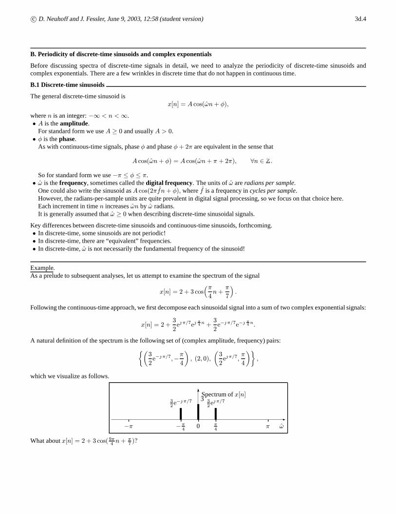
Example.As a prelude to subsequent analyses, let us attempt to examine the spectrum of the signal
x[n] = 2 + 3 cos(π4n+π
7
).
Following the continuous-time approach, we first decompose each sinusoidal signal into a sum of two complex exponential signals:
x[n] = 2 +3
2e π/7e
π4 n +
3
2e− π/7e−
π4 n.
A natural definition of the spectrum is the following set of (complex amplitude, frequency) pairs:{(3
2e− π/7,−
π
4
), (2, 0),
(3
2e π/7,
π
4
)},
which we visualize as follows.
-ω0−π ππ
4−π4
6Spectrum ofx[n]3 32e π/73
2e− π/7
What aboutx[n] = 2 + 3 cos(9π4 n+π7 )?
c© D. Neuhoff and J. Fessler, June 9, 2003, 12:58 (student version) 3d.5
The preceding example is simple enough, but now consider plotting the spectrum of the continuous-time signal
x(t) = 2 + cos
(2π1
5t+π
4
)+ cos
(2π1
5t−π
4
).
This signal has two terms with the same frequency so those two terms must becombined(using phasors) before plotting thespectrum:x(t) = 2 +
√2 cos
(2π 15 t
). Here it is “easy” to see which terms must be combined.(Picture)
In discrete time, there can be many sinusoids with having equivalent frequencies that must be combined before plotting a spectrum!
Periodicity of discrete-time sinusoids
Fact B1The discrete-time sinusoidal signalA cos(ωn+φ) is periodic if and only if ω2π is a rational number,i.e., if and only if we can writethefrequency ω in the formω = 2πM/N whereM andN are integers.
If the rational numberM/N is reduced so that the numerator and denominator have no common factors (except unity), then thefundamental period is the denominatorN of the rational number.
In contrast, recall that for continuous-time signals,everysinusoid is periodic, and thefundamental period is simply the reciprocalof the frequency in Hz, and the frequency of a sinusoid is also its fundamental frequency.
DerivationRecall the definition of periodicity:
A signalx[n] isN -periodic if and only ifx[n+N ] = x[n] , ∀n ∈ Z.
Thefundamental periodN0 is the smallest such period.
Let us apply the definition to see when a discrete-time sinusoid is periodic. We want to know when there is anN such that
A cos(ω(n+N) + φ) = A cos(ωn+ φ), ∀n ∈ Z.
SinceA cos(ω(n+ N) + φ) = A cos(ωn+ ωN + φ), we see that the above equality holds when and only whenωN = M · 2π,for some integerM , or equivalently, when and only whenω = 2πMN . In other words,ω must be2π times a rational number.
Let us now find the fundamental period ofA cos(ωn + φ). If the sinusoid is periodic, thenω = 2πKL
for some integersK andL.In this case, the sinusoid is periodic with periodN = L or 2L or 3L or . . ., because for any such value ofN , ωN = 2πKLN is aninteger multiple of2π.
What is the smallest period? If we eliminate any common factors ofK andL, we can writeω = 2πK′
L′, whereK ′ andL′ have no
common factors except unity (1). By the same argument as before,A cos(ωn+ φ) is periodic with periodL′. This is the smallestpossible period, so it is the fundamental period.
Example
(a)A cos(2π 12n) is periodic with fundamental periodN0 = 2. The frequency of this signal isω = π radians per sample.
(b)A cos(2π 35n) is periodic with fundamental periodN0 = 5. The frequency of this sinusoid isω = 2π 35 =65π.
Notice that (b) has higher frequency than (a), yet (b) also has a longer fundamental period than (a).This could not happen with continuous-time signals!
(c)A cos(2π 45n) is periodic fundamental periodN0 = 5. The frequency of this sinusoid isω = 2π 45 =85π.
Note that (b) and (c) have different frequencies, but the same fundamental period.This could not happen with continuous-time signals!
(d)A cos(2n+ π/2) is not periodic becauseω = 2π 1π
is not2π times a rational number.
(e)A cos(1.6πn) is periodic with fundamental periodN0 = 5, becauseω = 1.6π = 2π(0.8) = 2π 45 .

c© D. Neuhoff and J. Fessler, June 9, 2003, 12:58 (student version) 3d.6
Equivalent frequencies
Recall that phaseφ and phaseφ+ 2π are “equivalent” in the sense that the following signals are equal:
A cos(ωn+ φ) = A cos(ωn+ φ+ 2π), ∀n ∈ Z.
As we now demonstrate, in the case of discrete-time sinusoids, there are also equivalentfrequencies.
Fact B2Frequencyω and frequencyω + 2π are “equivalent” in the sense that the following signals are equal:
A cos((ω + 2π)n+ φ) = A cos(ωn+ 2πn+ φ) = A cos(ωn+ φ), ∀n ∈ Z.
This is another phenomena that is different for discrete time than for continuous time.(The above derivation will not work if you try to replacen ∈ Zwith t ∈ R.)
Because of these equivalences, we usually limit attention to0 ≤ ω < 2π for sinusoidal signals.
Example. The signalscos(15πn+
π3
)andcos
(115 πn+
π3
)areidenticalbecause15π and 115 π areequivalent frequencies.
Explanation:
cos
(11
5πn+
π
3
)= cos
([1
5π +10
5π
]n+π
3
)= cos
(2π1
5n+ 2πn+
π
3
)= cos
(2π1
5n+π
3
).
Example. The signalscos(15πn+
π3
)andcos
(95πn−
π3
)areidenticalbecause− 15π and 95π areequivalent frequencies.
Explanation:
cos
(9
5πn−
π
3
)= cos
(9
5πn− 2πn−
π
3
)= cos
((9
5π − 2π
)n−π
3
)= cos
(−1
5πn−
π
3
)= cos
(1
5πn+
π
3
), ∀n ∈ Z.
The following figure illustrates the difference between the continuous-time case and the discrete-time case.
0 2 4 6 8 10
−1
−0.5
0
0.5
1
x1(t) = cos(π/5*t + π/3)
0 2 4 6 8 10
−1
−0.5
0
0.5
1
x2(t) = cos(11*π/5*t + π/3)
0 2 4 6 8 10
−1
−0.5
0
0.5
1
x3(t) = cos(9*π/5*t − π/3)
t
0 2 4 6 8 10
−1
−0.5
0
0.5
1
x1[n] = cos(π/5*n + π/3)
0 2 4 6 8 10
−1
−0.5
0
0.5
1
x2[n] = cos(11*π/5*n + π/3)
0 2 4 6 8 10
−1
−0.5
0
0.5
1
x3[n] = cos(9*π/5*n − π/3)
n
c© D. Neuhoff and J. Fessler, June 9, 2003, 12:58 (student version) 3d.7
B.2 Complex exponentials
The general discrete-time complex exponential isAe φe ωn.
• A is the amplitude. We useA ≥ 0.• φ is the phase.
Phaseφ and phaseφ+ 2π are equivalent in the sense that
Ae (φ+2π)e ωn = Ae φe 2πe ωn = Ae φe ωn.
So we use−π ≤ φ ≤ π.• ω is the frequency. Its units are radians per sample. One could also write the exponential asAe φe 2πfn, wheref is frequency
in cycles per sample.We allow ω to be positive or negative. This is because we like to think of a cosine as being the sum of complex exponentialshaving positive and negative frequencies.
A cos(ωn+ φ) =1
2Ae φe ωn +
1
2Ae− φe− ωn.
Periodicity of discrete-time complex exponentials
Below, we list the periodicity properties of discrete-time exponentials. They are the same as discussed previously for discrete-timesinusoids.
Fact B3Ae φe ωn is periodic when and only whenω is 2π times a rational number.
If ω = 2πM/N whereM andN are integers having no common divisors, then the fundamental period isN .
Fact B4Frequencyω and frequencyω + 2π are equivalent in the sense that
Ae φe (ω+2π)n = Ae φe ωne 2π = Ae φe ωn.
Discussion.
What do we make of the surprising fact that frequencyω and frequencyω+2π are equivalent? We conclude that when we considerdiscrete-time sinusoids or complex exponentials, we can restrict frequencies to an interval of width2π, since any other frequenciesoutside this interval will be redundant.• Sometimes people restrict attention to[−π, π) or (−π, π] or perhaps[−π, π].• Sometimes people restrict attention to[0, 2π).• We’ll do a bit of both.
C. The spectrum of a finite sum of discrete-time sinusoids
Our discussion of how to assess a spectrum parallels the discussion for continuous-time sinusoids. We begin by considering signalsthat are finite sums of sinusoids. However, because of the possibility of equivalent frequencies, there are a couple of key differencesin how discrete-time and continuous-time spectra are assessed.

c© D. Neuhoff and J. Fessler, June 9, 2003, 12:58 (student version) 3d.8
C.1. Example
A discrete-time signal that is a finite sum of sinusoids:
x[n] = 3 + 2 cos
(1
5πn+
π
3
)+ 5 cos
(4
3πn
)+ 2 cos
(9
5πn−
π
3
).
As in the continuous-time approach, we expressx[n] as a sum of complex exponentials:
x[n] = 3 +(e π/3e
15πn + e− π/3e−
15πn)+
(5
2e43πn +
5
2e−
43πn
)+(e− π/3e
95πn + e π/3e−
95πn).
It would now seem natural to identify the spectrum as the following set of complex ampli-tude and frequency pairs:{(e π/3,−
9
5π
),
(5
2,−4
3π
),
(e− π/3,−
1
5π
), (3, 0),
(e π/3,
1
5π
),
(5
2,4
3π
), . . .
},
and to draw the spectrum as follows.
-
ω0 15π π 4
3π 9
5π−1
5π−π−4
3π−9
5π
6Spectrum ofx[n]??
3
e π/3
52
e− π/3e− π/3
52
e π/3
However, some of these exponentials have equivalent frequencies, so the above plot ismisleading! Specifically,• Frequencies−15π and95π are equivalent because they differ by2π (or a multiple of2π).• Frequencies−95π and 15π, are equivalent for the same reason.• Frequency4
3π is equivalent to−2
3π, and−4
3π is equivalent to2
3π.
We combine all exponentials having equivalent frequencies (using phasor addition) intoa single exponential component. In doing so, we get to choose which of the equivalentfrequencies the resulting exponential component will have.There are two possible conventions:• Two-sided spectra. Exponential components have frequencies in the interval[−π, π].• One-sided spectra. Exponential components have frequencies in the interval[0, 2π).
Choosing between these two conventions is mainly a matter of taste.
c© D. Neuhoff and J. Fessler, June 9, 2003, 12:58 (student version) 3d.9
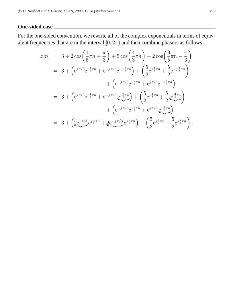
One-sided case
For the one-sided convention, we rewrite all of the complex exponentials in terms of equiv-alent frequencies that are in the interval[0, 2π) and then combine phasors as follows:
x[n] = 3 + 2 cos
(1
5πn+
π
3
)+ 5 cos
(4
3πn
)+ 2 cos
(9
5πn −
π
3
)= 3 +
(e π/3e
15πn + e− π/3e−
15πn)+
(5
2e43πn +
5
2e−
43πn
)+(e− π/3e
95πn + e π/3e−
95πn)
= 3 +(e π/3e
15πn + e− π/3 e
95πn︸ ︷︷ ︸)+
(5
2e43πn +
5
2e23πn︸ ︷︷ ︸)
+(e− π/3e
95πn + e π/3 e
15πn︸ ︷︷ ︸)
= 3 +(2e π/3︸ ︷︷ ︸ e 15πn + 2e− π/3︸ ︷︷ ︸ e 95πn)+
(5
2e43πn +
5
2e23πn
).
c© D. Neuhoff and J. Fessler, June 9, 2003, 12:58 (student version) 3d.10
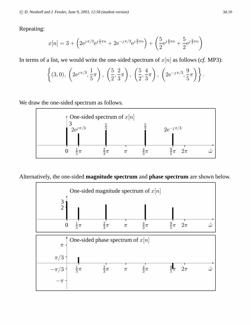
Repeating:
x[n] = 3 +(2e π/3e
15πn + 2e− π/3e
95πn)+
(5
2e43πn +
5
2e23πn
)
In terms of a list, we would write the one-sided spectrum ofx[n] as follows (cf. MP3):{(3, 0),
(2e π/3,
1
5π
),
(5
2,2
3π
),
(5
2,4
3π
),
(2e− π/3,
9
5π
)}.
We draw the one-sided spectrum as follows.
-
ω0 π 2π15π
23π
43π
95π
6One-sided spectrum ofx[n]32e π/3
52
52 2e− π/3
Alternatively, the one-sidedmagnitude spectrumandphase spectrumare shown below.
-
ω0 π 2π15π
23π
43π
95π
6
One-sided magnitude spectrum ofx[n]
23
-
ωπ 2π15π
23π
43π
95π
6One-sided phase spectrum ofx[n]π
−π
π/3
−π/3

c© D. Neuhoff and J. Fessler, June 9, 2003, 12:58 (student version) 3d.11
Two-sided case
For the two-sided convention, we rewrite all of the complex exponentials in terms of theequivalent frequencies that are in the interval[−π, π] and then combine phasors as follows:
x[n] = 3 +(e π/3e
15πn + e− π/3e−
15πn)+
(5
2e43πn +
5
2e−
43πn
)+(e− π/3e
95πn + e π/3e−
95πn)
= 3 +(e π/3e
15πn + e− π/3e−
15πn)+
(5
2e−
23πn︸ ︷︷ ︸+52 e 23πn︸ ︷︷ ︸
)+(e− π/3 e−
15πn︸ ︷︷ ︸+e π/3 e 15πn︸ ︷︷ ︸)
= 3 +(2e π/3︸ ︷︷ ︸ e 15πn + 2e− π/3︸ ︷︷ ︸ e− 15πn)+
(5
2e43πn +
5
2e−
43πn
).
In terms of a list, we express thetwo-sided spectrumas follows:{(5
2,−2
3π
),
(2e− π/3,−
1
5π
), (3, 0),
(2e π/3,
1
5π
),
(5
2,2
3π
)}.
We draw the two-sided spectrum as follows.
-
ω0 π−π −15π 1
5π−2
3π 2
3π
6Two-sided spectrum ofx[n]
3
2e π/32e− π/3
52
52
Alternatively, we could draw the the magnitude spectrum and the phase spectrum.
Compare the one-sided and two-sided spectra above to see where the spectra lines go!• One-sided spectra correspond naturally to the DFT.• Two-sided spectra correspond naturally to the continuous-time case.

c© D. Neuhoff and J. Fessler, June 9, 2003, 12:58 (student version) 3d.12
C.2. Spectrum of a general sum of discrete-time sinusoids
More generally, consider a signal of the form
x[n] = A0 +
N ′∑k=1
Ak cos(ωkn+ φk)
= A0 +A1 cos(ω1n+ φ1) + · · ·+AN ′ cos(ωN ′n+ φN ′),
whereN ′,A0, A1, . . . , AN , ω1, . . . , ωN , φ1, . . . , φN , are parameters that specifyx[n]. We now rewrite this in several ways. First,using Euler’s formula, we rewritex[n] as
x[n] = X0 +N ′∑k=1
Re{Xke
ωkn}
where the phasor corresponding toAk cos(ωkn+ φk) is
Xk = Ake φk .
(Xk is a complex number.)
Second, using the inverse Euler formula, we rewrite this as
x[n] = X0 +
N ′∑k=1
[1
2Xke
ωkn +1
2X?ke
− ωkn
].
To simplify this, we write it as follows:
x[n] =
N ′∑k=−N ′
βke− ωkn
where
β0 = X0 = A0, βk =
{12Xk, k = 1, . . . , N
′
12X
?k , k = −1, . . . ,−N
′.
Finally, as needed we combine terms with equivalent frequencies, to obtain
x[n] =N∑
k=−N
αke− ωkn,
where{ωk} is a set of frequencies with values between−π andπ, andαk is the phasor that is the sum of the appropriateβk ’scorresponding to frequencies that are equivalent toωk:
αk =∑
j : ωj=ωk+m2π, m∈Z
βj .
Note thatα−k = α
?k, |α−k| = |αk|, \α−k = −\αk.
We now use this expression to make the following definition.
Definition. The spectrum of a sum of sinusoids.
Thetwo-sided spectrumis
{(α−N , ω−N) , . . . , (α−1, ω−1) , (α0, 0) , (α1, ω1) , . . . , (αN , ωN)}
= {(α?N ,−ωN) , . . . , (α?1,−ω1) , (α0, 0) , (α1, ω1) , . . . , (αN , ωN)} .
Theone-sided spectrumis
{(α0, 0) , (α1, ω1) , . . . , (αN , ωN) (α−N , ω−N + 2π) , . . . , (α−1, ω−1 + 2π) , }
= {(α0, 0) , (α1, ω1) , . . . , (αN , ωN ) (α?N , 2π − ωN) , . . . , (α
?1, 2π − ω1) , } .

c© D. Neuhoff and J. Fessler, June 9, 2003, 12:58 (student version) 3d.13
Notes.As with continuous-time spectra, we have the following properties.• The spectrum,i.e., one of these lists, is considered to be a simpler, more compact representation of the signalx[n], i.e., just a
few numbers.• The “spectrum” is often called thefrequency-domain representationof the signal. In contrast,x[n] is called thetime-domain
representationof the signal.• The termαke ωkn is called thecomplex exponential componentor spectral componentof x[n] at frequencyωk.• To obtain a useful visualization, we often plot the spectrum. That is, for eachk, we draw aspectral line at frequencyωk with
height equal to|αk|, and we label the line with the value ofαk, which is in general is complex.• Alternatively, we sometimes separate the spectrum into magnitude and phase parts. For example, the two-sided versions of these
are shown below.Themagnitude spectrumis
{(|α−N |, ω−N ) , . . . , (|α−1|, ω−1) , (|α0|, 0) , (|α1|, ω1) , . . . , (|αN |, ωN )}
= {(|αN |,−ωN) , . . . , (|α1|,−ω1) , (|α0|, 0) , (|α1|, ω1) , . . . , (|αN |, ωN )} ,
which is even symmetric.Thephase spectrumis
{(\α−N , ω−N ) , . . . , (\α−1, ω−1) , (\α0, 0) , (\α1, ω1) , . . . , (\αN , ωN)}
= {(−\αN ,−ωN) , . . . , (−\α1,−ω1) , (\α0, 0) , (\α1, ω1) , . . . , (\αN , ωN )} ,
which is odd symmetric.And we might draw separate plots of the magnitude and phase. That is, for eachk, the magnitude plot has a line of height|αk|at frequencyωk, and the phase plot has a line of height\αk at frequencyωk.• Often, but certainly not always, we are more interested in the magnitude spectrum than the phase spectrum.
Example. Determine what signalx[n] (in standard form) has the spectrum shown below.
-ω0 π 2ππ/3 3
4π54π 5π/3
6One-sided spectrum ofx[n]
21e π/4 e− π/4
3e− π/2 3e π/2
Reading off the exponential components, we see that
x[n] = 2 + e π/4eπ3 n + 3e− π/2e
3π4 n + 1e πn + 3e π/2e
5π4 n + e− π/4e
5π3 n
= 2 +(e π/4e
π3 n + e− π/4e
5π3 n)+(3e− π/2e
3π4 n + 3e π/2e
5π4 n)+ e πn
= 2 +(e π/4e
π3 n + e− π/4e−
π3 n)+(3e− π/2e
3π4 n + 3e π/2e−
3π4 n)+ e πn
= 2 + 2 cos(π
3n+ π/4) + 6 cos(
3π
4n− π/2) + cos(πn).
Notice the use of equivalent frequencies in the middle of the derivation:
e5π3 n = e−
π3 n.
Is x[n] periodic? Yes, because all of the frequencies of the sinusoidal components are2π times a rational number.
What is the period ofx[n]? The three components have periods: 6, 8, and 2, the LCM of which isN0 = 24.
0 10 20 30 40 50 60 70−5
0
5
10
n
x[n]
c© D. Neuhoff and J. Fessler, June 9, 2003, 12:58 (student version) 3d.14
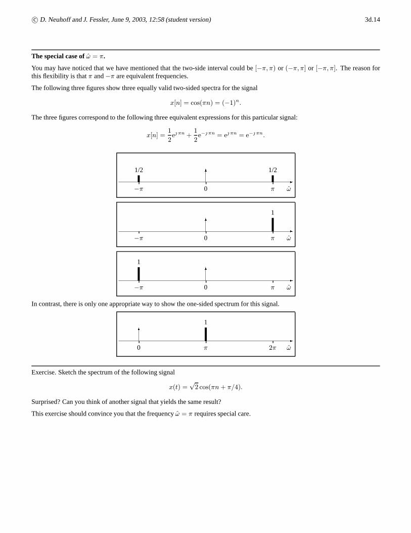
The special case ofω = π.
You may have noticed that we have mentioned that the two-side interval could be[−π, π) or (−π, π] or [−π, π]. The reason forthis flexibility is thatπ and−π are equivalent frequencies.
The following three figures show three equally valid two-sided spectra for the signal
x[n] = cos(πn) = (−1)n.
The three figures correspond to the following three equivalent expressions for this particular signal:
x[n] =1
2e πn +
1
2e− πn = e πn = e− πn.
-ω0 π−π
6 1/21/2
-ω0 π−π
6
1
-ω0 π−π
6
1
In contrast, there is only one appropriate way to show the one-sided spectrum for this signal.
-ω0 π 2π
6
1
Exercise. Sketch the spectrum of the following signal
x(t) =√2 cos(πn+ π/4).
Surprised? Can you think of another signal that yields the same result?
This exercise should convince you that the frequencyω = π requires special care.
c© D. Neuhoff and J. Fessler, June 9, 2003, 12:58 (student version) 3d.15
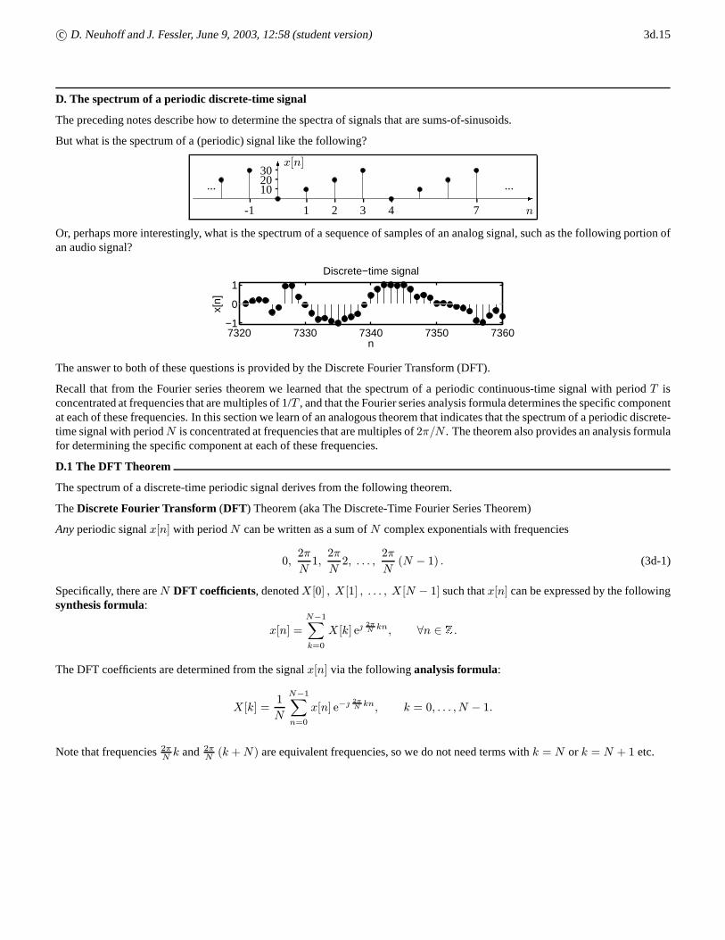
D. The spectrum of a periodic discrete-time signal
The preceding notes describe how to determine the spectra of signals that are sums-of-sinusoids.
But what is the spectrum of a (periodic) signal like the following?
-n-1 1 2 3 4 7
6x[n]
102030
......
Or, perhaps more interestingly, what is the spectrum of a sequence of samples of an analog signal, such as the following portion ofan audio signal?
7320 7330 7340 7350 7360−1
0
1
n
x[n]
Discrete−time signal
The answer to both of these questions is provided by the Discrete Fourier Transform (DFT).
Recall that from the Fourier series theorem we learned that the spectrum of a periodic continuous-time signal with periodT isconcentrated at frequencies that are multiples of 1/T , and that the Fourier series analysis formula determines the specific componentat each of these frequencies. In this section we learn of an analogous theorem that indicates that the spectrum of a periodic discrete-time signal with periodN is concentrated at frequencies that are multiples of2π/N . The theorem also provides an analysis formulafor determining the specific component at each of these frequencies.
D.1 The DFT Theorem
The spectrum of a discrete-time periodic signal derives from the following theorem.
TheDiscrete Fourier Transform (DFT) Theorem (aka The Discrete-Time Fourier Series Theorem)
Anyperiodic signalx[n] with periodN can be written as a sum ofN complex exponentials with frequencies
0,2π
N1,2π
N2, . . . ,
2π
N(N − 1) . (3d-1)
Specifically, there areN DFT coefficients, denotedX [0] , X [1] , . . . , X [N − 1] such thatx[n] can be expressed by the followingsynthesis formula:
x[n] =N−1∑k=0
X [k] e2πN kn, ∀n ∈ Z.
The DFT coefficients are determined from the signalx[n] via the followinganalysis formula:
X [k] =1
N
N−1∑n=0
x[n] e−2πN kn, k = 0, . . . , N − 1.
Note that frequencies2πNk and 2π
N(k +N) are equivalent frequencies, so we do not need terms withk = N or k = N + 1 etc.

c© D. Neuhoff and J. Fessler, June 9, 2003, 12:58 (student version) 3d.16
Notes
• We will derive this theorem later. Unlike the Fourier Series Theorem, its derivation is well within the scope of this class!
• The terme2πN kn appearing in the synthesis formula is thecomplex exponential component(equivalently, thespectral
component) of x[n] at frequency2πNk.
• The theorem says thatanyperiodic discrete-time signal can be represented as the sum of at mostN complex exponentialcomponents with frequencies coming from the set
{0, 2πN1, 2πN2, . . . , 2π
N(N − 1)
}.
This means that the spectrum of a periodic signal with periodN is concentrated at these frequencies (or a subset thereof).
• The synthesis formula is very much like the synthesis formula for the Fourier series of a continuous-time periodic signal,except that only afinite number of frequencies/exponential components are used. This stems from the fact that for discrete-time complex exponentials, every frequency outside the range[0, 2π) is equivalent to some frequency within the range[0, 2π).
Furthermore, all of the information about a discrete-time periodic signal is contained in theN signal values over one period:x[0] , . . . , x[N − 1] . SinceN values is enough to describex[n], it is logical to expect that we should need at mostNfrequency components to describex[n]. (If more thanN frequency components were needed, then the spectrum of a signalwould be a less concise description of the signal that the time-domain values, which would greatly diminish its utility!)
• For periodic signals, it is natural then to use the following list as the definition of theone-sided spectrum:{(X [0] , 0) ,
(X [1] ,
2π
N1
),
(X [2] ,
2π
N2
), . . . ,
(X [N − 1] ,
2π
N(N − 1)
).
}Thus, finding the spectrum of a periodic discrete-time signal involves finding its period and finding theX [k]’s.
We could also define atwo-sided spectrumfrom the DFT coefficients. However, as described later, the two-sided spectrumis somewhat messier.
• When we compute theX [k]’s using the analysis formula, there is no need to combine exponential components with equivalentfrequencies, as we did previously when finding the spectrum of a finite sum of sinusoids. In essence, the DFT analysisformula has already done this for us.
• To aid the understanding of the synthesis and analysis formulas, it can be useful to view them in long form:
Thesynthesis formula:
x[n] =N−1∑k=0
X [k] e2πN kn = X [0] +X [1] e
2πN 1n +X [2] e
2πN 2n + · · ·+X [N − 1] e
2πN (N−1)n.
Theanalysis formula:
X [k] =1
N
N−1∑n=0
x[n] e−2πN kn =
1
N
(x[0] + x[1] e−
2πN 1n + x[2] e−
2πN 2n + · · ·+ x[N − 1] e−
2πN (N−1)n
).
Notice how similar these formulas are; they only differ by the 1/N and by the sign in the exponent.
An elementary example of computing these formulas is given in Section D.2.
• The frequency2π/N is called thefundamental or first harmonic frequency.The frequency2π
Nk is called thekth-harmonic frequency.
The component at frequency2π/N is called thefundamental or first harmonic component.The component at frequency2π
Nk is called thekth-harmonic component.
• The analysis formula may be viewed as operating on a periodic signalx[n] (actually, just onx[0] , . . . , x[N − 1]) and pro-ducingN DFT coefficientsX [0] , . . . , X [N − 1]. This operation is considered to be atransform of the signalx[n] into theset of coefficientsX [0] , . . . , X [N − 1]. This is whytransform appears in the nameDiscrete Fourier Transform.
Similarly, the synthesis formula may be viewed as operating on Fourier coefficientsX [0] , . . . , X [N − 1] and producing asignalx[n]. This operation is considered to be aninverse transform.

c© D. Neuhoff and J. Fessler, June 9, 2003, 12:58 (student version) 3d.17
• It is customary to writeX [k] as a shorthand for{X [0] , . . . , X [N − 1]}, just as the notation “x[n]” usually refers to an entiresignal. So there are two possible meanings for the notation “X [k]”: it could mean thekth coefficient, or it could mean theentire set ofN coefficients.
• The termDiscrete Fourier Transform (DFT) commonly refers both to theprocessof applying the analysis formula as wellas to the coefficientsX [k] that result from this process. For example, people often say “X [k] is the DFT ofx[n].”
• The process of applying the analysis formula tox[n] is often called “finding/taking the DFT ofx[n]” or, sometimes, “DFT’ingx[n].” Similarly, the process of synthesizingx[n] from the DFT coefficientsX [k] is often called “finding/taking the inverseDFT ofX [k],” or “inverse DFT’ingX [k].”
• It is traditional to useX [k] to denote the DFT ofx[n], Y [k] to denote the DFT ofy[n], X1[k] to denote the DFT ofx1[n],and so on.
• WhenN is a power of 2,i.e., N = 2m for somem ∈ N, there is fast algorithm for computing the DFT (i.e., the analysisformula), called thefast Fourier transform (FFT). Because the synthesis formula and the analysis formula are so verysimilar, a slight variation on the FFT algorithm, called theinverse FFT can also be used to compute the synthesis formula.These algorithms have enabled the widespread use of the DFT in the analysis, design, and implementation of signals andsystems. The FFT is one of the most important tools of modern signal processing and is at the core of many of the ubiquitousdigital signal processing devices around us.
• The FFT algorithm is available in MATLAB through the commandsfft andifft . If you use these commands, be awareof a factor ofN difference between our definition of the DFT and MATLAB ’s convention.• To compute our definition of the DFT (analysis), use:X = 1/N * fft(x)• To compute our definition of the inverse DFT (synthesis), use:x = N * ifft(X)
• Since the summand in the analysis formula is periodic with periodN , the limits of the summation could be replaced withany interval of lengthN .
• If a signal has periodN , then it also has period 2N and period 3N and so on. Thus, when applying DFT analysis, we canchoose which periodN to use. Usually, but certainly not always, we chooseN to be thefundamental period. When wewant to specify explicitly the value ofN used, we will say “theN -point DFT.” As discussed in Section D.4, using 2N or3N (etc.) instead ofN does not change the spectrum.
• The DFT Theorem applies both to real signals and to complex signals.
• Observe that according to the analysis formula, coefficientX [k] is computed by correlatingx[n] with the complex exponen-tial e−
2πN kn and then dividing byN . ThisN is the energy of one period of the exponential:
N−1∑n=0
∣∣∣e− 2πN kn∣∣∣2 = N−1∑n=0
1 = N.
Suggested reading. The discussion of “signal components” at the end of Section IIIB of the “Introduction to Signals” byDLN. This section will help one to understand why the analysis formula has the form that it has.
In the terminology of that discussion:• X [k] e
2πN kn is the component ofx[n] that is likee
2πN kn,
• X [k]measures the similarity ofx[n] to the exponential.
• The reader is encouraged to review the discussion of Fourier series for continuous-time signals and observe the similaritieswith the DFT for discrete-time periodic signals. The principal differences are• t is replaced byn• T is replaced byN• The DFT synthesis formula has onlyN terms.• The DFT analysis formula uses a sum rather than an integral.

c© D. Neuhoff and J. Fessler, June 9, 2003, 12:58 (student version) 3d.18
DFT Examples
Example. Find the spectrum of the signal
x[n] = 5 + 3(−1)n + 8 cos(2n+ 3).
Before jumping into the DFT, we must ask: isx[n] periodic? Here
x[n] = 5 + 3 cos(πn) + 8 cos(2π1
πn+ 3).
Since1/π is irrational, this signal is not periodic. So we cannot apply the DFT. But we can still determine the spectrum ofx[n].
-ω0 π 2π2 2π − 2
6One-sided spectrum ofx[n]
5
34e 3 4e− 3
Be sure to think about why the component atπ is “3” rather than “3/2.”
Equivalent frequencies revisited
The most important uses of equivalent frequencies are the following
e− ωn = e (2π−ω)n e−2πN kn = e
2πN (N−k).
Computing the DFT
There are three basic methods for “manually” determining the DFT of a signal:• using the DFT analysis formula,• matching the DFT coefficients “by inspection,”• combining the above with DFT properties.
The same techniques also work for the inverse DFT since it is almost the same formula!
Recall theN -point DFT formulas:
Analysis:X [k] =1
N
N−1∑n=0
x[n] e−2πN kn Synthesis:x[n] =
N−1∑k=0
X [k] e2πN kn.
Example. Find the spectrum of the following signal. (Using theanalysis formula.)
-n-1 0 1 2 3 4 7
6x[n]
51525
......
This signal is periodic. Its fundamental period isN0 = 4, so we chooseN = N0 = 4 for the DFT.

c© D. Neuhoff and J. Fessler, June 9, 2003, 12:58 (student version) 3d.19
Applying the analysis formula:
X [k] =1
4
3∑n=0
x[n] e−2π4 kn =
1
4
[x[0] e−
2π4 k0 + x[1] e−
2π4 k1 + x[2] e−
2π4 k2 + x[3] e−
2π4 k3]
=1
4
[15 + 25e−
2π4 k + 15e− πk + 5e−
2π4 k3]=
14 (15 + 25 + 15 + 5), k = 014 (15− 25j − 15 + 5j), k = 114 (15− 25 + 15− 5), k = 214 (15 + 25j − 15− 5j), k = 3
=
15, k = 0−5j, k = 10, k = 25j, k = 3.
The frequencies that correspond to these DFT coefficients are multiples of2π/4. So in list form the spectrum is{(15, 0) ,
(5e− π/2, π/2
),(5e π/2, 3π/2
)}.
Graphically, the spectrum of this signal is the following.
-ω0 π/2 π 3π/2 2π
6One-sided spectrum ofx[n]
155e− π/2 5e π/2
It is also useful to be able to expressx[n] as a sum of complex exponentials or sinusoids. Applying the synthesis formula:
x[n] =3∑k=0
X [k] e2π4 kn = X [0] e
2π4 0n +X [1] e
2π4 1n +X [2] e
2π4 2n +X [3] e
2π4 3n
= 15 + 5e− π/2e2π4 n + 5e−π/2e
2π4 3n = 15 + 5e− π/2e
2π4 n + 5e−π/2e−
2π4 n = 15 + 10 cos(
2π
4n−π
2),
where we used the fact that3π/2 and−π/2 are equivalent frequencies. In this case, one could also recognize the final expressionfor x[n] directly from its spectrum.
Example. (Usingcoefficient matching.)
Determine the 32-point DFT the following signalx[n] = 20 sin2(3π8 n).
TheN -point DFT allows us to express aN -periodic signal as a sum ofN complex exponentials:
x[n] =
N−1∑k=0
X [k] e2πN kn = X [0] +X [1] e
2πN 1n +X [2] e
2πN 2n + · · ·+X [N − 1] e
2πN (N−1)n. (3d-2)
If we can find such an expression directly, then we do not need to use the analysis formula.In this case, apply an inverse Euler identity:
x[n] = 20 sin2(3π
8n) = 20
(e3π8 n − e−
3π8 n
2
)2
= 20
(e
2π32 6n − e−
2π32 6n
2
)2= 5
(2− e
2π32 12n − e−
2π32 12n
)= 10− 5e
2π32 12n − 5e−
2π32 12n = 10− 5e
2π32 12n − 5e
2π32 20n,
where in the last line we used the fact that− 2π32 12 and 2π32 20 are equivalent frequencies. Considering the final form, comparing to(3d-2) we see that the32-point DFT ofx[n] is given by:
X [k] =
10, k = 0−5, k = 12−5, k = 200, otherwise.
c© D. Neuhoff and J. Fessler, June 9, 2003, 12:58 (student version) 3d.20
We see that this signal has a DC term and two other complex exponential terms.
Example. (Using theanalysis formula.)
Determine the 32-point DFT the following signaly[n] = (1/5)n. Note that this is an infinite duration signal, so we are onlycomputing the DFT of a segment of it for0 ≤ n ≤ 31. We choseN = 32 here simply for illustration.
Substitutey[n] into the analysis formula and use a geometric series formula to help simplify:
Y [k] =1
32
31∑n=0
(1/5)n e−2π32 kn =
1
32
31∑n=0
((1/5) e−
2π32 k)n
=1
32
1−((1/5) e−
2π32 k)32
1− (1/5) e−2π32 k
=1
32
1− 1/532
1− (1/5) e−2π32 k.
A plot of the magnitude spectrum shows that this signal has nearly the same power at all frequencies, with a bit more at the lowerfrequencies.
Example. (Usingproperties.)
Determine the 32-point DFT the following signalz[n] = 40 sin2(3π8 (n− 4)) + 7(1/5)n.
We see thatz[n] = 2x[n− 4] + 7y[n] . Theshift property of the DFT is the following.If s[n] = x[n− n0], thenS[k] = X [k] e−
2πN kn0 .
Thus, using the shift property and thelinearity of the DFT, we see that
Z[k] = 2X [k] e−2π32 k4 + 7Y [k] =
20 + 7321−1/532
1−(1/5) , k = 0
−10e−2π32 4·12 + 7
321−1/532
1−(1/5) e−2π3212, k = 12
−10e−2π32 (4·20) + 7
321−1/532
1−(1/5) e−2π3220, k = 20
732
1−1/532
1−(1/5) e−2π32k, otherwise.
So what?
After we know how to compute the DFT of a signal, what can we do? There are an enormous number of applications; the DFT andits fast computational version, the FFT, are the foundation for much of signal processing.• As demonstrated in lecture, we can perform audio signal compression by discarding frequency components with small DFT
coefficients. This is the essence of how MP3 works.• In lab you will see how to use the DFT to remove a contaminating tone from an audio signal.• If we start with a continuous-time signal and sample it to form a discrete-time signal and then compute the DFT of that discrete-
time signal, then we will soon discuss how the DFT coefficients are related to the spectrum of the original continuous-timesignal. This is how instruments like digital oscilloscopes display the (approximate) spectrum of continuous-time signals.
c© D. Neuhoff and J. Fessler, June 9, 2003, 12:58 (student version) 3d.21
Example. (Using theanalysis formula, a long example.)
Determine the 32-point DFT the following signalx[n] = | sin(3π8 n)|. Note that the period of this signal isN0 = 8, but there arestill reasons why one might want to compute theN -point DFT forN larger thanN0; we choseN = 32 here simply for illustration.
Now substitutex[n] into the analysis formula and use Euler to help simplify:
X [k] =1
32
31∑n=0
| sin(3π
8n)| e−
2π32 kn =
1
32
[15∑n=0
sin(3π
8n) e−
2π32 kn −
31∑n=16
sin(3π
8n) e−
2π32 kn
]
=1
32
[15∑n=0
e3π8 n − e−
3π8 n
2e−
2π32 kn −
31∑n=16
e3π8 n − e−
3π8 n
2e−
2π32 kn
]
=1
64
[15∑n=0
(e2π32 6n − e−
2π32 6n
)e−
2π32 kn −
31∑n=16
(e
2π32 6n − e−
2π32 6n
)e−
2π32 kn
]
=1
64
[15∑n=0
(e2π32 (6−k)n − e−
2π32 (6+k)n
)−
31∑n=16
(e
2π32 (6−k)n − e−
2π32 (6+k)n
)]
=1
64
[15∑n=0
e2π32 (6−k)n −
15∑n=0
e2π32 (26−k)n −
31∑n=16
e2π32 (6−k)n +
31∑n=16
e2π32 (26−k)n
].
Apparently we will have to consider the casesk = 6 andk = 26 separately. Forother values ofk we apply a geometric seriesformula to find:
X [k] =1
64
1−
(e
2π32 (6−k)
)161− e
2π32 (6−k)
−1−
(e
2π32 (26−k)
)161− e
2π32 (26−k)
− (−1)k1− (−1)k
1− e2π32 (6−k)
+ (−1)k1− (−1)k
1− e2π32 (26−k)
=1− (−1)k
32
[1
1− e2π32 (6−k)
−1
1− e2π32 (26−k)
]=1− (−1)k
32·1− e
2π32 (26−k) − [1− e
2π32 (6−k)]
[1− e2π32 (6−k)][1− e
2π32 (26−k)]
=1− (−1)k
32
e2π32 (6−k) − e
2π32 (−6−k)
[1− e2π32 (6−k)][1− e
2π32 (−6−k)]
=1− (−1)k
16
e−2π32k sin(2π32 6)
1− e2π32 (6−k) − e
2π32 (−6−k) + e
2π32 (−2k)
=1− (−1)k
16
sin(2π32 6)
e2π32 k − e
2π32 6 − e
2π32 (−6) + e
2π32 (−k)
=1− (−1)k
8
sin(3π8 )
cos(2π32 k)− cos(3π8 ).
This is too messy to serve as a classroom example. However, the original signalx[n] is real and even, so the above manipulationsshow that with enough simplification, we can indeed find DFT coefficients that are real.
Fork = 6 we have
X [6] =1
64
[15∑n=0
1−15∑n=0
e2π32 20n −
31∑n=16
1 +
31∑n=16
e2π32 20n
]= 0
and similarlyX [26] = 0. So our final answer is
X [k] =
0, k = 6, 26
1− (−1)k
8
sin(3π8 )
cos(2π32 k)− cos(3π8 )
otherwise.=
0, k even1
4
sin(3π8 )
cos(2π32 k)− cos(3π8 )
k odd.
Admittedly this problem would be easier to solve (approximately) using MATLAB .

c© D. Neuhoff and J. Fessler, June 9, 2003, 12:58 (student version) 3d.22
D.3 Derivation of the DFT
To demonstrate the validity of the theorem, we will first show that when the analysis formula forX [k] is substituted into thesynthesis formula, the result isx[n]. We will then show that when the synthesis formula holds, the analysis formula is the one andonly way to determine the coefficients.
These demonstrations rely on the following fact, which we will derive before demonstrating the validity of the DFT Theorem. Thisfact will also be useful at other times in the course.
Fact D1N−1∑n=0
e2πN (k−m)n =
{N, k = m, k = m±N, k = m± 2N, . . .0, otherwise.
Derivation.• Case 1. Whenk = m + lN for l ∈ Z, the exponent of each term is 0 or an integer multiple of2π, making each term equal 1.
Hence, in this case∑N−1n=0 e
2πN (k−m)n = N.
• Case 2. Whenk 6= m+ lN for every integerl, to simplify notation, letz = e2πN (k−m). Notice thatz 6= 1 in this case. Using
this definition and applying the finite geometric series formula:
N−1∑n=0
e2πN (k−m)n =
N−1∑n=0
zn =1− zN
1− z=1− e
2πN (k−m)N
1− z=1− e 2π(k−m)
1− z=1− 1
1− z= 0,
since the exponent in numerator is times a multiple of2π.
Derivation of the DFT Theorem
Substituting the analysis formula forX [k] into the synthesis formulas gives
N−1∑k=0
X [k] e2πN kn =
N−1∑k=0
[1
N
N−1∑n′=0
x[n′] e−2πN kn
′
]e
2πN kn
usingn′ in analysis formula sincen already used in synthesis formula
=1
N
N−1∑n′=0
x[n′]
[N−1∑k=0
e2πN k(n−n
′)
]rearranging terms
=1
Nx[n]N = x[n] if n = 0, . . . , N − 1, using Fact D1.
Specifically, the rightmost sum equals 0 when the exponent is nonzero,i.e., whenn′ 6= n, and equalsN when the exponent is zero,i.e., whenn′ = n. Therefore,x[n′] is multiplied by 0 whenn′ 6= n, and byN whenn′ = n.
So, we have just shown that if we apply the analysis formula to any signalx[n], then we when apply the synthesis formula to theresultingX [k]’s, we will get back thex[n]’s that we started with forn = 0, . . . , N − 1.
But could there beotherX [k]’s that also could be used to synthesize the signalx[n]? The answer is “no” as shown in the nextargument.
Finally, we show that if the synthesis formula holds, the coefficients must be calculated via the analysis formula. Suppose we havesomeX [k]’s for which the synthesis formula holds,i.e.,
x[n] =
N−1∑k=0
X [k] e2πN kn, n = 0, . . . , N − 1.
We want to show that theseX [k]’s must be those that come from the analysis formula.
We correlate both sides of this equation withe2πN k
′n. That is, we first multiply both sides of the above synthesis formula by(e
2πN k
′n)?= e−
2πN k
′n as follows
x[n] e−2πN k
′n =
[N−1∑k=0
X [k] e2πN kn
]e−
2πN k
′n.

c© D. Neuhoff and J. Fessler, June 9, 2003, 12:58 (student version) 3d.23
Since this equality holds forn = 0, . . . , N − 1, we now sum over all these values ofn:
N−1∑n=0
x[n] e−2πN k
′n =
N−1∑n=0
[N−1∑k=0
X [k] e2πN kn
]e−
2πN k
′n
=
N−1∑k=0
X [k]
[N−1∑n=0
e2πN (k−k
′)n
]rearranging terms
= X [k′]N,
where the last equality is due to Fact D1 again. Specifically, the rightmost sum equals 0 when the exponent is not zero,i.e., whenk 6= k′, and equalsN when the exponent is zero,i.e., whenk = k′. Therefore,X [k] is multiplied by 0 whenk 6= k′, and byNwhenk = k′. Rearranging the last equality and usingk in place ofk′ yields
X [k] =1
N
N−1∑n=0
x[n] e−2πN kn,
which is the analysis formula given in the DFT Theorem.

c© D. Neuhoff and J. Fessler, June 9, 2003, 12:58 (student version) 3d.24
D.4 Properties of the DFT
This section lists a number of useful properties of the DFT.
D1. UniquenessThere is a one-to-one relationship between periodic signals with periodN and sets of DFT coefficients. Specifically, for any givensignalx[n], the analysis formula gives the unique set of coefficients from which the synthesis formula yieldsx[n].
This implies that the DFT coefficients can sometimes be found by means other than the analysis formula,e.g., inspection. That is,if by some means you findX [k] such that
x[n] =
N−1∑k=0
X [k] e2πN kn,
then thisX [k] is necessarily the DFT that would be computed by the analysis formula.
Similarly, for any given set of DFT coefficientsX [k], the synthesis formula gives the unique signalx[n] with periodN from whichthe analysis formula yieldsX [k]. That is, if by some means you find a signalx[n] such that
X [k] =1
N
N−1∑n=0
x[n] e−2πN kn,
then that signalx[n] is the one and only signal havingX [k] as its coefficients.
Another statement of the one-to-oneness is that ifx1[n] andx2[n] are distinct periodic signals,i.e., x1[n] 6= x2[n] for at least onevalue ofn, each with periodN , then for at least onek,X1[k] 6= X2[k].
D2. Mean valueX [0] is the mean or DC value ofx[n].
This is because
X [0] =1
N
N−1∑n=0
x[n] e−2πN 0n =
1
N
N−1∑n=0
x[n] = M(x) ,
D3. Summation intervalFor aN -periodic signalx[n], one can compute the DFT coefficients by summing over any time interval of lengthN .
X [k] =1
N
N−1∑n=0
x[n] e−2πN kn =
1
N
m+N−1∑n=m
x[n] e−2πN kn ∀m ∈ Z.
D4. Conjugate symmetry(important)When the signalx[n] is real,
X [N − k] = X∗[k] , k = 1, . . . , N − 1
andX [0] = X∗[0] soX [0] is real.
This shows that if one knowsX [k] for k = 0, . . . , N/2, then one can easily find the remainingX [k]’s. This “redundancy” is oftenexploited in digital implementations to reduce memory requirements.
Note thatX [N − k] is the spectral component at frequency2πN(N − k), which is equivalent to frequency− 2π
Nk.
Derivation. (This property does not apply to complex signals!)
X∗[k] =
[1
N
N−1∑n=0
x[n] e−2πN kn
]?=1
N
N−1∑n=0
x∗[n] e2πN kn
=1
N
N−1∑n=0
x[n] e2πN kn becausex[n] is real sox∗[n] = x[n]
=1
N
N−1∑n=0
x[n] e−2πN (N−k)n because2π
Nk and− 2π
N(N − k) are equivalent frequencies
= X [N − k] .
c© D. Neuhoff and J. Fessler, June 9, 2003, 12:58 (student version) 3d.25
D5. Sinusoids(important)Conjugate pairs of coefficients synthesize a sinusoid When the signalx[n] is real,
X [k] e2πN kn +X [N − k] e
2πN (N−k)n = X [k] e
2πN kn +X∗[k] e−
2πN kn
= 2|X [k] | cos(2π
Nkn+ \X [k]).
Thus, when looking at a spectrum, one should “see” sinusoidal signal components, one for each conjugate pair of coefficients.
D6. LinearitySupposex[n] andy[n] are periodic with periodN and haveX [k] andY [k] as theirN -point DFTs, respectively. Then theN -pointDFT of s[n] = αx[n] + βy[n] is S[k] = αX [k] + βY [k].
Similarly, if X [k] andY [k] are sequences of lengthN with inverse DFTs given byx[n] andy[n], then the inverse DFT ofαX [k]+βY [k] is αx[n] + βy[n].
The derivations of these properties are left as exercises.
D7. Parseval’s theoremFor a real or complex signalx[n] that is periodic with periodN , we can computer the average power in the time domain or in thefrequency domain as follows:
signal average power= MS(x) =1
N
N−1∑n=0
|x[n] |2 =N−1∑k=0
|X [k] |2.
Recall that the average power of aN -periodic signalx[n] is
MS(x) = limM→∞
=1
2M + 1
M∑n=−M
|x[n] |2 =1
N
N−1∑n=0
|x[n] |2.
Derivation.
MS(x) =1
N
N−1∑n=0
|x[n] |2 =1
N
N−1∑n=0
x[n]x∗[n]
=1
N
N−1∑n=0
x[n]
[N−1∑k=0
X [k] e2πN kn
]?synthesis formula=
1
N
N−1∑n=0
x[n]
[N−1∑k=0
X∗[k] e−2πN kn
]
=
N−1∑k=0
X∗[k]
[1
N
N−1∑n=0
x[n] e−2πN kn
]rearranging
=
N−1∑k=0
X∗[k]X [k] by the analysis formula
=N−1∑k=0
|X [k] |2.
Example. (Theimpulse train signal.)
x[n] =
{A, n = 0,±N,±2N, . . .0, otherwise.
(Picture)
X [k] =1
N
N−1∑k=0
x[n] e−2πN kn =
1
NA =
A
N(Picture) .
Time domain:MS(x) = 1NA2. Frequency domain:MS(x) =
∑N−1k=0 |X [k] |
2 =∑N−1k=0
(AN
)2= N
(AN
)2= A2/N.

c© D. Neuhoff and J. Fessler, June 9, 2003, 12:58 (student version) 3d.26
The following properties will be emphasized less in this class.
D8. Choice of periodSupposex[n] is periodic with periodN , supposeX [k] is theN -point DFT ofx[n], and supposeX ′[k] is the 2N-point DFT ofx[n].Then,
X ′[k] =
{X [k/2] , k = 0, 2, 4, . . . , 2N − 20, otherwise.
This means that the (one-sided) spectrum based on the 2N -point DFT is the same as that based on theN -point DFT. For exampleif N is even, the spectrum based on the 2N -point DFT is{
(X ′[0] , 0) ,
(X ′[2] ,
2π
N2
), . . .
(X ′[2N − 2] ,
2π
N(2N − 2)
)}
=
{(X [0] , 0) ,
(X [1] ,
2π
N1
), . . .
(X [N − 1] ,
2π
N(N − 1)
)},
which is the one-sided spectrum based on theN -point DFT.
The derivation is left as an exercise.
D9. Time shiftIf x[n] has DFTX [k], thens[n] = x[n− n0] has DFT coefficients
S[k] = X [k] e−2πN kn0 .
This shows, not surprisingly, that a time shift causes a phase shift of each spectral component, where the phase shift is proportionalto the frequency of the component. The derivation is left as an exercise.
D10. Frequency shiftIf x[n] has DFTX [k], theny[n] = x[n] e
2πN mn has DFT coefficients1
Y [k] = X [k −m] .
This shows that multiplying a signal by a complex exponential has the effect of shifting the spectrum of the signal. The derivationis left as an exercise.
D11. Time scalingThis is not as straightforward as in the continuous-time case and will not be discussed here, except to indicate that ifm is a positiveinteger, theny[n] = x[nm] is a subsampledversion ofx[n], which is well defined. (In contrast, the expressionx[n/m] is notdefined for all values ofn.) See EECS 451 for thorough coverage.
D12. Finite sums?Since the DFT synthesis formula is a finite sum, we can compute the values “exactly” (to within the precision of our computers),unlike in the case of continuous-time signals where we usually have to make finite approximations to the infinite sums.
However, for data compression problems such as MP3 audio coding, we can save memory by discarding small DFT coefficientsthereby reducing the finite sum to an even smaller number of terms, at the expense of imperfect signal synthesis.
D13. Technicalities?Since the sums in the synthesis and analysis formulas are finite, no technical conditions are needed as are required for the Fourierseries.
D14. Real and even signalsIf x[n] is real and even (x[−n] = x[n]), then the DFT coefficients are real.
Example. (Picture) y[n] = 24x[n]− 16x[n− 4] wherex[n] is the impulse train worked out earlier withA = 1 andN = 8.
Y [k] = 24X [k]− 16X [k] e−2π8 [4]k = 24 18 − 16
18 (−1)
k = 3− 2(−1)k =
{1, k even5, k odd
(Picture)
Sox[n] = 1 + 10 cos(π4n) + 2 cos(π2n) + 10 cos(
3π4 n) + cos(πn).
1There is a subtle technicality here; the expressionk −mmust be interpreted moduloN .
c© D. Neuhoff and J. Fessler, June 9, 2003, 12:58 (student version) 3d.27
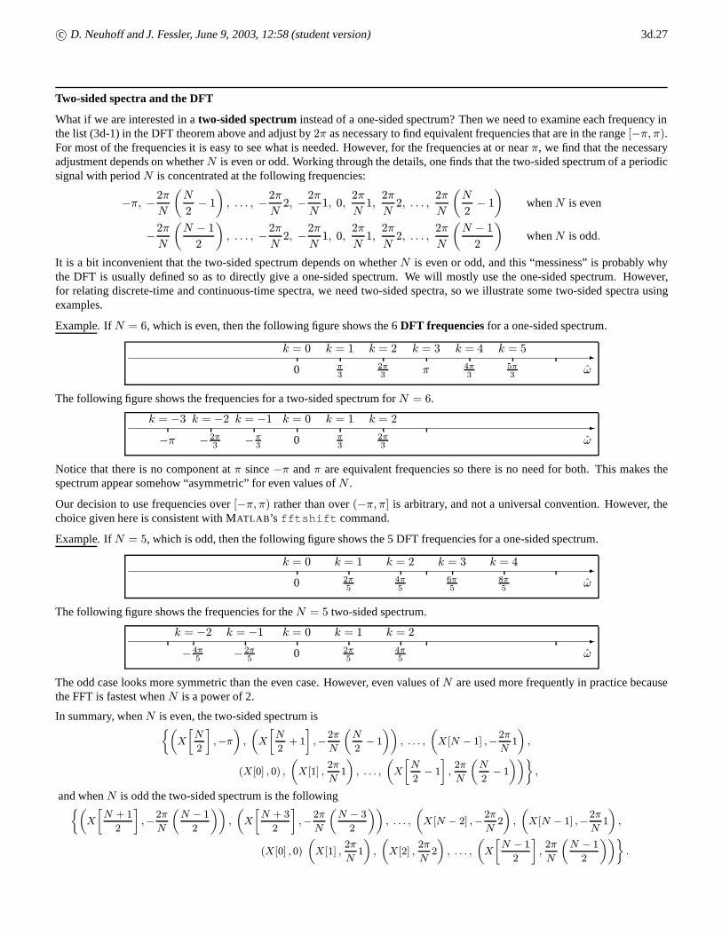
Two-sided spectra and the DFT
What if we are interested in atwo-sided spectruminstead of a one-sided spectrum? Then we need to examine each frequency inthe list (3d-1) in the DFT theorem above and adjust by2π as necessary to find equivalent frequencies that are in the range[−π, π).For most of the frequencies it is easy to see what is needed. However, for the frequencies at or nearπ, we find that the necessaryadjustment depends on whetherN is even or odd. Working through the details, one finds that the two-sided spectrum of a periodicsignal with periodN is concentrated at the following frequencies:
−π, −2π
N
(N
2− 1
), . . . , −
2π
N2, −
2π
N1, 0,
2π
N1,2π
N2, . . . ,
2π
N
(N
2− 1
)whenN is even
−2π
N
(N − 1
2
), . . . , −
2π
N2, −
2π
N1, 0,
2π
N1,2π
N2, . . . ,
2π
N
(N − 1
2
)whenN is odd.
It is a bit inconvenient that the two-sided spectrum depends on whetherN is even or odd, and this “messiness” is probably whythe DFT is usually defined so as to directly give a one-sided spectrum. We will mostly use the one-sided spectrum. However,for relating discrete-time and continuous-time spectra, we need two-sided spectra, so we illustrate some two-sided spectra usingexamples.
Example. If N = 6, which is even, then the following figure shows the 6DFT frequenciesfor a one-sided spectrum.
-ω0 π
32π3 π 4π
35π3
k = 0 k = 1 k = 2 k = 3 k = 4 k = 5
The following figure shows the frequencies for a two-sided spectrum forN = 6.
-ω−π − 2π3 −π3 0 π
32π3
k = 0 k = 1 k = 2k = −3 k = −2 k = −1
Notice that there is no component atπ since−π andπ are equivalent frequencies so there is no need for both. This makes thespectrum appear somehow “asymmetric” for even values ofN .
Our decision to use frequencies over[−π, π) rather than over(−π, π] is arbitrary, and not a universal convention. However, thechoice given here is consistent with MATLAB ’s fftshift command.
Example. If N = 5, which is odd, then the following figure shows the 5 DFT frequencies for a one-sided spectrum.
-ω0 2π
54π5
6π5
8π5
k = 0 k = 1 k = 2 k = 3 k = 4
The following figure shows the frequencies for theN = 5 two-sided spectrum.
-ω− 4π5 − 2π5 0 2π
54π5
k = −2 k = −1 k = 0 k = 1 k = 2
The odd case looks more symmetric than the even case. However, even values ofN are used more frequently in practice becausethe FFT is fastest whenN is a power of 2.
In summary, whenN is even, the two-sided spectrum is{(X
[N
2
],−π
),
(X
[N
2+ 1
],−2π
N
(N
2− 1
)), . . . ,
(X[N − 1] ,−
2π
N1
),
(X[0] , 0) ,
(X[1] ,
2π
N1
), . . . ,
(X
[N
2− 1
],2π
N
(N
2− 1
))},
and whenN is odd the two-sided spectrum is the following{(X
[N + 1
2
],−2π
N
(N − 1
2
)),
(X
[N + 3
2
],−2π
N
(N − 3
2
)), . . . ,
(X[N − 2] ,−
2π
N2
),
(X[N − 1] ,−
2π
N1
),
(X[0] , 0)
(X[1] ,
2π
N1
),
(X[2] ,
2π
N2
), . . . ,
(X
[N − 1
2
],2π
N
(N − 1
2
))}.

c© D. Neuhoff and J. Fessler, June 9, 2003, 12:58 (student version) 3d.28
E. The spectra of segments of a signal
Question: How can we assess the spectrum of a signal that is not periodic?
For example, what if the signal has finite support? Or what if the signal has infinite support, but is not periodic?
Observation: The DFT analysis formula uses only a finite segment of a signal.
Signals with finite support
To assess the spectrum of a signalx[n] with finite support{n1, . . . , n2}, we can apply the DFT analysis formula directly to thesignal over its support interval.
Let us begin by definingx(t) to be a periodic signal that equalsx[n] on the interval{n1, . . . , n2} and simply repeats this behavioron other intervals of the same length. That is, letN = n2 − n1 + 1, and let
x[n] =
∞∑m=−∞
x[n−mN ] .
The signalx[n] is called theperiodic extensionof x[n]. Its periodN is the support length ofx[n].
Example. Here is a signal with finite support.
-n0 1 2 3 4 5
6x[n]
51525
Here is its periodic extension.
-n-2 -1 0 1 2 3 4 5 6 7
6x[n]
51525
......
Returning to the general case, taking theN -point DFT ofx[n], we find
x[n] =
N−1∑k=0
X [k] e2πN kn (synthesis formula)
where
X [k] =1
N
n2∑n=n1
x[n] e−2πN kn (analysis formula),
and where we have used the fact that the analysis formula can have summation limits that cover any interval of lengthN .
Now we note that sincex[n] = x[n] for n1 ≤ n ≤ n2,
we also have
x[n] =N−1∑k=0
X [k] e2πN kn, n1 ≤ n ≤ n2, (synthesis formula)
X [k] =1
N
n2∑n=n1
x[n] e−2πN kn (analysis formula).
Thus we may view the two formulas above as synthesis and analysis formulas for a spectral representation ofx[n]. The synthesisformula shows that, on its support interval,x[n] can be viewed as the sum of complex exponentials with frequencies that are

c© D. Neuhoff and J. Fessler, June 9, 2003, 12:58 (student version) 3d.29
multiples of2π/N . The analysis formula shows how to find the spectral components. It is important to note that the synthesisformula yieldsx[n] only in the support interval. Outside the support interval it yieldsx[n], rather thanx[n] = 0.
In summary, for a signal with finite support, we take the (one-sided) spectrum to be{(X [0] , 0) ,
(X [1] ,
2π
N1
),
(X [2] ,
2π
N2
), . . . ,
(X [N − 1] ,
2π
N(N − 1)
).
}
just as we did for periodic signals.
Note. Though we have introduced the DFT as fundamentally applying to periodic signals and secondarily applying to signals withfinite support, some people take the opposite point of view, which is also valid.
Aperiodic signals with infinite support
A common approach to assessing the spectrum of an aperiodic signal with infinite support is to choose an integerN , divide thetime axis into segments[0, N − 1], [N, 2N − 1], [2N, 3N − 1], etc, and apply the above DFT approach to each segment. Thisyields a sequence of spectra, one for each segment.
Since the signal is not periodic, the data within each segment will be different. Thus the spectrum will differ from segment tosegment. For example, the spectrum of the signal
x[n] = cos(3.2n)
is shown below for two different segments of lengthN = 128.
0 1 2 3 4 5 6 70
0.05
0.1
0.15
0.2
0.25
0.3
0.35
radians/sample
0 1 2 3 4 5 6 70
0.05
0.1
0.15
0.2
0.25
0.3
0.35
radians/sample
Notice that these two spectra are quite similar. Notice also that even though the signal is a pure sinusoidal signal, whose spectrum,according to the discussion of Section C, is concentrated entirely at frequencies 3.2 and -3.2, the spectra above show a couple ofstrong components in the vicinity of 3.2 and -3.2, and small components at other harmonic frequencies. This may be viewed asbeing due to the fact that we are using harmonic frequencies to synthesize a sinusoid whose frequency is not harmonic. It may alsobe viewed as being due to the fact that these spectra are actually the spectra of a periodic extensionx[n] of x[n]. A more thoroughdiscussion, which would derive the actual form of the spectra shown above, is left to future courses.
The fact that we now have two different ways of assessing the spectrum of signals such asx[n] = cos(3.2n), as in Section C andas discussed here, may seem somewhat disconcerting. But this is reflective of the fact that, as mentioned earlier, thespectrum is abroad concept, like “economy” or “health,” that has no simple, universal definition.
c© D. Neuhoff and J. Fessler, June 9, 2003, 12:58 (student version) 3d.30
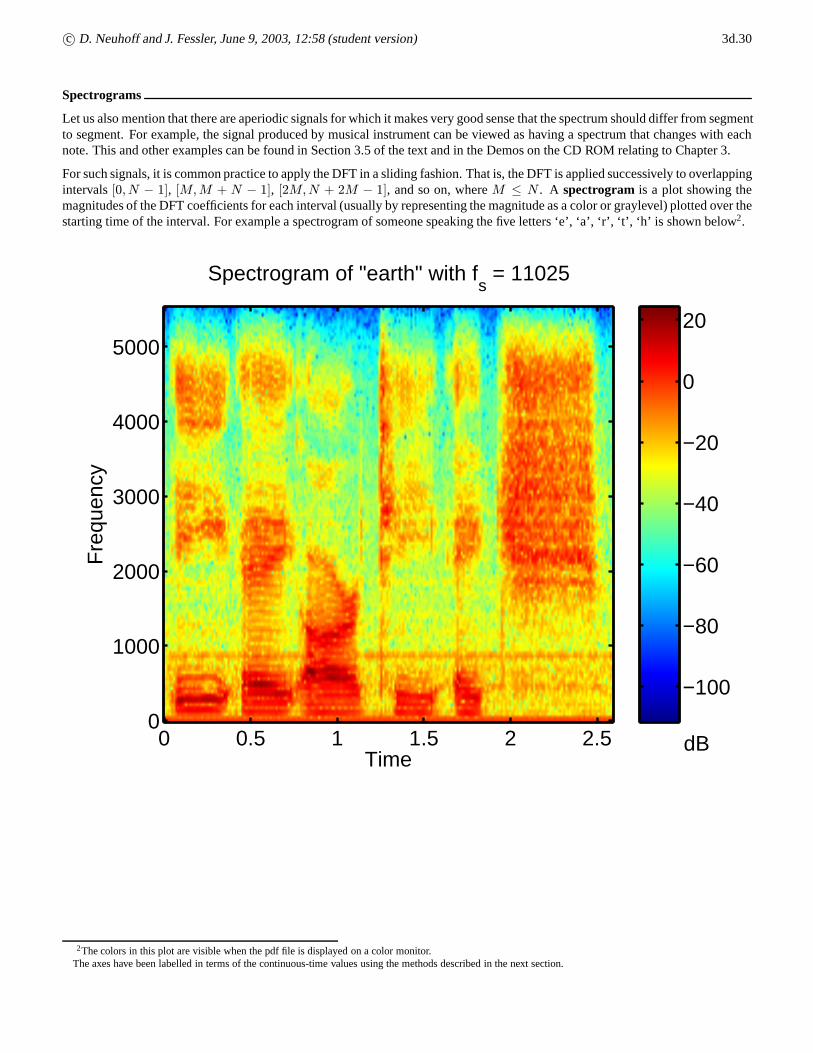
Spectrograms
Let us also mention that there are aperiodic signals for which it makes very good sense that the spectrum should differ from segmentto segment. For example, the signal produced by musical instrument can be viewed as having a spectrum that changes with eachnote. This and other examples can be found in Section 3.5 of the text and in the Demos on the CD ROM relating to Chapter 3.
For such signals, it is common practice to apply the DFT in a sliding fashion. That is, the DFT is applied successively to overlappingintervals[0, N − 1], [M,M + N − 1], [2M,N + 2M − 1], and so on, whereM ≤ N . A spectrogram is a plot showing themagnitudes of the DFT coefficients for each interval (usually by representing the magnitude as a color or graylevel) plotted over thestarting time of the interval. For example a spectrogram of someone speaking the five letters ‘e’, ‘a’, ‘r’, ‘t’, ‘h’ is shown below2.
Time
Fre
quen
cy
Spectrogram of "earth" with fs = 11025
dB0 0.5 1 1.5 2 2.50
1000
2000
3000
4000
5000
−100
−80
−60
−40
−20
0
20
2The colors in this plot are visible when the pdf file is displayed on a color monitor.The axes have been labelled in terms of the continuous-time values using the methods described in the next section.

c© D. Neuhoff and J. Fessler, June 9, 2003, 12:58 (student version) 3d.31
Example
Here is another aperiodic signal
x[n] = cos(2π
3(n+ 100e−n/100)).
We compute the DFT over the 1st block of 64 samples and then over the 2nd block of 64 samples.
It is clearly from the DFT coefficients that the second block has more of its power at higher frequencies, as expected in this casefrom the nature of the signal.
0 20 40 60 80 100 120−1
−0.5
0
0.5
1
n
x[n]
0 20 40 60−1
−0.5
0
0.5
1
x 1[n]
First block
0 20 40 600
5
10
15
20
X1[k
]
80 100 120−1
−0.5
0
0.5
1Second block
n
x 2[n]
0 20 40 600
5
10
15
20
k
X2[k
]

c© D. Neuhoff and J. Fessler, June 9, 2003, 12:58 (student version) 3d.32
F. The relationship between the spectrum of a continuous-time signal and that of its samples
Frequently, we are often interested in the spectrum of some continuous-time signal, but for practical reasons, we sample the signaland work with the resulting discrete-time signal. If possible, we would like to be able to deduce the spectrum of the continuous-timesignal from that of the discrete-time signal. This section shows how this can be done, at least approximately.
Example. We first illustrate the idea with the simplest possible example: a continuous-time sinusoidal signal.
x(t) = cos(2πf0t)→ SampleTs → x[n] = x(nTs)
Using the sampling relationship:x[n] = x(nTs) = cos(2πf0(nTs)) = cos(2πf0Tsn)
so we see that a continuous-time sinusoid of frequencyf0 becomes, after sampling, a discrete-time sinusoid of frequency
ω0 = 2πf0Ts = 2πf0
fs. (3d-3)
Example. Supposef0 = 20Hz, andTs = 0.02s sofs = 50Hz. And ω0 = 2π20/50 = 4π/5.
Then the spectra ofx(t) andx[n] are as follows.
-f [Hz]-25 -20 0 20 25
6Spectrum ofx(t)
1/21/2
-ω0−π π4π
5− 4π5
6Spectrum ofx[n]
1/21/2
What if we do not have an equation for the signal?
In the preceding example, we have an analytical expression forx(t) so we can draw “theoretical” spectra. In practice, if we havea “mystery signal”x(t) whose spectrum we would like to examine, we must take a finite number,N , of samples of that signal,compute the DFTX [k] of those samples, and then somehow relate theX [k]’s to the spectrum original signalx(t).
The nature of what that DFT-based spectrum will look like will depend somewhat on the value ofN that is chosen.
The following figure shows the DFT coefficients for various choices forN for the preceding example.
Consider first the choiceN = 40, which is a multiple of the fundamental period ofx[n] which isN0 = 5 in the preceding example.Then
x[n] = cos(2π2
5n) =
1
2e
2π5 2n +
1
2e−
2π5 2n =
1
2e
2π40 16n +
1
2e−
2π16 40n
so by coefficient matching we see that the 40-point DFT ofx[n] is given by
X [k] =
1/2, k = 161/2, k = 240, otherwise.
But what ifN = 41? Then we cannot use coefficient matching sinceM/41 6= 2/5 for any integerM .
But we can still find the 41-point DFT ofx[n] usingfft , the result of which is shown in the figure. Now instead of a “clean line”we get peaks at 16 and 24 but the peaks are a bit “smeared out.” Using a largerN , likeN = 401 shown in the figure, tightens upthe lines.

c© D. Neuhoff and J. Fessler, June 9, 2003, 12:58 (student version) 3d.33
0 0.2 0.4 0.6 0.8−10
0
10
t
x(t)
DFT of sampled sinusoidal signal
0 10 20 30 400
1
2
3
|X[k
]|
N=40
0 10 20 30 400
1
2
3
|X[k
]|
N=41
0 100 200 300 4000
1
2
3
k
|X[k
]|
N=401
From the synthesis equation
x[n] =
N−1∑k=0
X [k] e2πN kn
we see that the frequency associated with thekth DFT coefficient is
ω =2π
Nk.
Combining this with the relationship (3d-3) we havef0/fs = k/N . However, this is only valid forω ≤ π. For ω > π we mustconsider the equivalent frequency between−π and0. In summary:
f =
{kNfs, k = 0, . . . , N/2− 1
N−kNfs, k = N/2, . . . , N − 1.
(3d-4)
These are the formulas that any “digital spectrum analyzer” must use when displaying the DFT coefficients of samples of acontinuous-time signal with the axes labeled in terms of Hz.
c© D. Neuhoff and J. Fessler, June 9, 2003, 12:58 (student version) 3d.34
Further analysis
For concreteness, consider a periodic continuous-time signalx(t) with periodT , and consider sampling it with sampling intervalTs � T . Then the resulting discrete-time signal is
x[n] = x(nTs) .
By the Fourier Series theorem,x(t)may be expressed as a sum of complex exponential components:
x(t) =
∞∑k=−∞
αke 2π kT t
where
αk =1
T
∫〈T 〉x(t) e− 2π
kT t dt.
Can we compute or approximate theαk ’s from the samples ofx(t), i.e., fromx[n]? This question is answered by the following.
Fact F1Let x(t) be a periodic signal with periodT , letx[n] = x(nTs) be the discrete-time signal formed by samplingx(t) with samplingintervalTs = T/N , whereN � 1, and letX [k] denote theN -point DFT ofx[n]. (It is easy to see thatx[n] is periodic with periodN .) Claim:
αk ≈ X [k] for k � N.
Derivation:
To see how theαk ’s can be approximated, we will use the fact that sinceTs � T , x(t) varies little over mostTs second intervals.Thus, it may be approximated with
x(t) ≈ x(nTs) = x[n] , for nTs ≤ t < nTs + Ts.
We will also use the following approximation, the validity of which is discussed shortly:
e− 2πkT t ≈ e− 2π
kT nTs = e−
2πN kn, whennTs ≤ t < nTs + Ts.
With these approximations, we now proceed by rewriting the integral in the analysis formula as a sum ofN integrals over intervalsof lengthTs seconds, whereN = T/Ts:
αk =1
T
∫ T0
x(t) e− 2πkT t dt
=1
T
N−1∑n=0
∫ nTs+TsnTs
x(t) e− 2πkT t dt integrating over short intervals
≈1
T
N−1∑n=0
∫ nTs+TsnTs
x[n] e−2πN kn dt using the above approximations
=1
T
N−1∑n=0
x[n] e−2πN kn
∫ nTs+TsnTs
dt rearranging terms
=1
T
N−1∑n=0
x[n] e−2πN knTs computing the integral
=1
N
N−1∑n=0
x[n] e−2πN kn usingN = T/Ts
= X [k] thekth coefficient inN -point DFT ofx[n].
This fact shows that thekth Fourier coefficientαk is approximately equal to thekth DFT coefficientX [k] in anN -point DFT ofx[n]. This means that the DFT coefficientX [k] indicates the presence inx(t) of the spectral component (cf. (3d-4)):
X [k] e 2πkT t at frequency
k
T=k
NTs=k
Nfs,
c© D. Neuhoff and J. Fessler, June 9, 2003, 12:58 (student version) 3d.35
wherefs = 1/Ts is the sampling frequency. In other words, the component at frequencyω = 2πNk in the discrete-time signalx[n]
represents a spectral component in the continuous-time signalx(t) at frequencykNfs.
On the other hand, the fact thatαk ≈ X [k] seems to contradict the fact that there are infinitely manyk’s for a continuous-timeperiodic signal, but only finitely manyX [k]’s. This apparent paradox is resolved by noting that the approximation
e− 2πkT t ≈ e−
2πN kn, whennTs ≤ t < nTs + Ts
is valid when and only when the exponential varies little within eachTs second interval. Since the exponential is periodic withperiodT/k, this approximation is valid when and only whenTs � T/k, or equivalently, when
k �T
Ts= N.
Thus we see that the approximationαk ≈ X [k] is valid only whenk � N . (Actually, it turns out to be fairly good as long ask < N/2.)
In summary, we have shown how to approximately compute the Fourier series coefficients{αk} of a continuous-time signal fromits samples. And the computation turns out to be the DFT!
We have also shown that the approximation is valid whenk � N = T/Ts. This indicates that where possible, one should choosethe sampling intervalTs to be small enough so that theαk ’s can be well approximated over whatever range of frequencies are ofinterest.
With this approximation for the Fourier series coefficients, one can now use the DFT coefficients to approximate the (two-sided)spectrum of the continuous-time signalx(t) as follows{(
X∗[K] ,−K
Nfs
), . . . ,
(X∗[1] ,−
1
Nfs
), (X [0] , 0) ,
(X [1] ,
1
Nfs
), . . . ,
(X [K] ,
K
Nfs
),
},
whereK is the largest value ofk for which we believeαk ≈ X [k]. Note that we are, in effect, approximating the spectrum ashaving no components above frequencyKfs.
Although we know the approximation is valid only fork � N , it is quite common to use the entire set of DFT coefficients in anapproximation for the spectrum ofx(t). Specifically, it is common to plot the one-sided spectrum{
(X [0] , 0) ,
(X [1] ,
1
Nfs
),
(X [2] ,
2
Nfs
), . . . ,
(X [N − 1] ,
N − 1
Nfs
),
}.
However, when interpreting such a plot, one must recall that such a spectrum is accurate only for values ofk � N . Moreover,whenk > N/2, the termX [k] = X∗[N − k]. Thus if anything, fork > N/2, the spectral line shown at frequencyk
Nfs is
indicative of what happens at frequency(N−k)N fs, not at what happens at frequencykN fs.
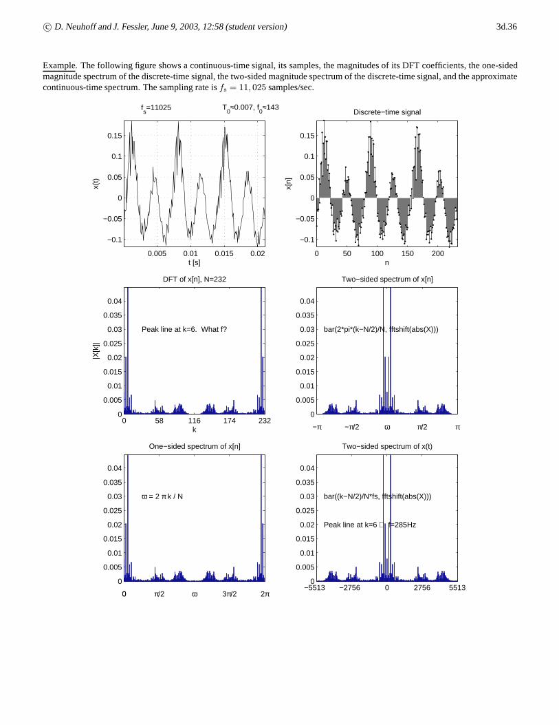
c© D. Neuhoff and J. Fessler, June 9, 2003, 12:58 (student version) 3d.36
Example. The following figure shows a continuous-time signal, its samples, the magnitudes of its DFT coefficients, the one-sidedmagnitude spectrum of the discrete-time signal, the two-sided magnitude spectrum of the discrete-time signal, and the approximatecontinuous-time spectrum. The sampling rate isfs = 11, 025 samples/sec.
0.005 0.01 0.015 0.02
−0.1
−0.05
0
0.05
0.1
0.15
t [s]
x(t)
fs=11025 T
0≈0.007, f
0≈143
0 50 100 150 200
−0.1
−0.05
0
0.05
0.1
0.15
n
x[n]
Discrete−time signal
0 58 116 174 2320
0.005
0.01
0.015
0.02
0.025
0.03
0.035
0.04
k
|X[k
]|
DFT of x[n], N=232
Peak line at k=6. What f?
0
0.005
0.01
0.015
0.02
0.025
0.03
0.035
0.04
One−sided spectrum of x[n]
0 π/2 3π/2 2π0 ω
ω = 2 π k / N
0
0.005
0.01
0.015
0.02
0.025
0.03
0.035
0.04
Two−sided spectrum of x[n]
π−π π/2−π/2 ω
bar(2*pi*(k−N/2)/N, fftshift(abs(X)))
−5513 −2756 0 2756 55130
0.005
0.01
0.015
0.02
0.025
0.03
0.035
0.04
Two−sided spectrum of x(t)
bar((k−N/2)/N*fs, fftshift(abs(X)))
Peak line at k=6 ⇒ f=285Hz

c© D. Neuhoff and J. Fessler, June 9, 2003, 12:58 (student version) 3d.37
G. Bandwidth
One of the primary motivations for assessing the spectrum of signal is to find the range of frequencies occupied by it. This rangeis often called the signal’s “band of spectral occupancy,” or, more simply, itsfrequency band. The width of the frequency band iscalled thebandwidth.
As one example, signals with non-overlapping spectra do not interfere with each other. So if we know the frequency band occupiedby each of a set of signals, we can determine if they interfere. As another example, certain communication media,e.g., a wire, limitpropagation to signals with spectral components in a certain range. If we know the frequency band occupied by a signal, we candetermine if it will propagate.
Most signals of practical interest, such as that shown in the previous section, have spectral components extending over a broadrange of frequencies. We are not really interested in the entire range of frequencies over which the spectrum is not zero. Ratherwe are interested in the range of frequencies over which the spectrum is “significantly large.” As such, we need a definition of“significantly large” to define the concepts of “frequency band” and “bandwidth.” There are a number of such definitions in use.The definition given below is based on one such definition.
Definition:
The “band of spectral occupancy” orfrequency band of a signalx[n] is the smallest interval of frequencies that includes allfrequencies at which the magnitude spectrum is at least one half as large as the maximum value of the magnitude spectrum.

c© D. Neuhoff and J. Fessler, June 9, 2003, 12:58 (student version) 3d.38
Signal compression
The following figure, discussed in detail in lecture, describes how discarding small frequency components can greatly reducestorage (like MP3) with only modest signal distortion.
2000 4000 6000 8000 10000 12000
−0.5
0
0.5
x[n]
Original audio signal, Fs=8192
8000 8050 8100 8150 8200−1
−0.5
0
0.5
1
0 5000 10000
200
400
600
800
k
|X[k
]|
Magnitude spectrum
12880 nonzero DFT coefficients
0 5000 100000
200
400
600
800
k
|Y[k
]|
Sparsified magnitude spectrum
2000 4000 6000 8000 10000 12000
−0.5
0
0.5
y[n]
Compressed audio signal, Fs=8192
562 nonzero DFT coefficients
with |X[k]| > 20
8000 8050 8100 8150 8200−1
−0.5
0
0.5
1
n
y[n]

c© D. Neuhoff and J. Fessler, June 9, 2003, 12:58 (student version) 3d.39
Noise removal by filtering with the DFT
Here are three (of many) applications of the DFT.• Signal compression (e.g., MP3, JPEG)• Digital spectrum analyzers (e.g., digital ’scopes)• Noise removal (filtering)
We have discussed the 1st two applications, now we turn to the third.
The following figure, discussed in detail in lecture, shows a signal with noise, and shows that removing the high frequency compo-nents can eliminate a lot of noise yet retain the dominant signal components.
0.005 0.01 0.015 0.02
−0.2
−0.1
0
0.1
0.2
0.3
t [s]
x 2(t)
Continuous−time signal with NOISE
fs=11025
0 50 100 150 200
−0.2
−0.1
0
0.1
0.2
0.3
n
x 2[n]
Discrete−time signal
RMS error = 0.09
0 58 116 174 2320
0.005
0.01
0.015
0.02
0.025
0.03
0.035
0.04
k
|X2[k
]|
DFT of x2[n], N=232
0
0.005
0.01
0.015
0.02
0.025
0.03
0.035
0.04
Two−sided spectrum of x2[n]
π−π π/2−π/2 ω
0
0.005
0.01
0.015
0.02
0.025
0.03
0.035
0.04
Two−sided spectrum of y[n]
π−π π/2−π/2 ω0 50 100 150 200
−0.1
−0.05
0
0.05
0.1
0.15
n
y[n]
Filtered discrete−time signal
RMS error = 0.03
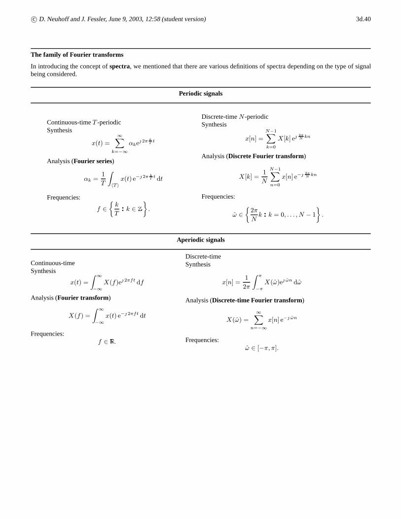
c© D. Neuhoff and J. Fessler, June 9, 2003, 12:58 (student version) 3d.40
The family of Fourier transforms
In introducing the concept ofspectra, we mentioned that there are various definitions of spectra depending on the type of signalbeing considered.
Periodic signals
Continuous-timeT -periodicSynthesis
x(t) =
∞∑k=−∞
αke 2π kT t
Analysis (Fourier series)
αk =1
T
∫〈T 〉x(t) e− 2π
kT t dt
Frequencies:
f ∈
{k
T: k ∈ Z
}.
Discrete-timeN -periodicSynthesis
x[n] =
N−1∑k=0
X [k] e2πN kn
Analysis (Discrete Fourier transform)
X [k] =1
N
N−1∑n=0
x[n] e−2πN kn
Frequencies:
ω ∈
{2π
Nk : k = 0, . . . , N − 1
}.
Aperiodic signals
Continuous-timeSynthesis
x(t) =
∫ ∞−∞X(f)e 2πft df
Analysis (Fourier transform )
X(f) =
∫ ∞−∞x(t) e− 2πft dt
Frequencies:f ∈ R.
Discrete-timeSynthesis
x[n] =1
2π
∫ π−πX(ω)e ωn dω
Analysis (Discrete-time Fourier transform)
X(ω) =
∞∑n=−∞
x[n] e− ωn
Frequencies:ω ∈ [−π, π].


![Aperiodic tilings [1ex]and substitutions - univ-orleans.fr€¦ · Aperiodic tilings and substitutions Nicolas Ollinger LIFO, Université d’Orléans Journées SDA2, ... Tilings](https://static.fdocuments.in/doc/165x107/5f1071477e708231d4492197/aperiodic-tilings-1exand-substitutions-univ-aperiodic-tilings-and-substitutions.jpg)


