
C. Aggarwal. A Survey of Uncertain Data Clustering Algorithms, In Data Clustering
26
Chapter 18 A Survey of Uncertain Data Clustering Algorithms Charu C. Aggarwal IBM T. J. Watson Research Center Yorktown Heights, NY 10598 [email protected] 18.1 Introduction ....................................................... 455 18.2 Mixture Model Clustering of Uncertain Data ........................ 457 18.3 Density Based Clustering Algorithms ............................... 458 18.3.1 FDBSCAN Algorithm ..................................... 458 18.3.2 FOPTICS Algorithm ...................................... 459 18.4 Partitional Clustering Algorithms ................................... 460 18.4.1 The UK-means Algorithm ................................. 460 18.4.2 The CK-Means Algorithm ................................. 461 18.4.3 Clustering Uncertain Data with Voronoi Diagrams .......... 462 18.4.4 Approximation Algorithms for Clustering Uncertain Data ... 462 18.4.5 Speeding up Distance Computations ....................... 463 18.5 Clustering Uncertain Data Streams ................................. 464 18.5.1 The UMicro Algorithm .................................... 464 18.5.2 The LuMicro Algorithm ................................... 469 18.5.3 Enhancements to Stream Clustering ........................ 469 18.6 Clustering Uncertain Data in High Dimensionality .................. 470 18.6.1 Subspace Clustering of Uncertain Data ..................... 471 18.6.2 UPStream: Projected Clustering of Uncertain Data Streams . 472 18.7 Clustering with the Possible Worlds Model ......................... 475 18.8 Clustering Uncertain Graphs ....................................... 475 18.9 Conclusions and Summary ......................................... 476 Bibliography ......................................................... 477 18.1 Introduction Many data sets which are collected often have uncertainty built into them. In many cases, the underlying uncertainty can be easily measured and collected. When this is the case, it is possible to use the uncertainty in order to improve the results of data mining algorithms. This is because the uncertainty provides a probabilistic measure of the relative importance of different attributes in data mining algorithms. The use of such information can enhance the effectiveness of data mining algorithms, because the uncertainty provides a guidance in the use of different attributes during the mining process. Some examples of real applications in which uncertainty may be used are as follows: • Imprecise instruments and hardware are sometimes used in order to collect the data. In such 455
Transcript of C. Aggarwal. A Survey of Uncertain Data Clustering Algorithms, In Data Clustering
Chapter 18
A Survey of Uncertain Data Clustering Algorithms
Charu C. Aggarwal
IBM T. J. Watson Research CenterYorktown Heights, NY [email protected]
18.1 Introduction . . . . . . . . . . . . . . . . . . . . . . . . . . . . . . . . . . . . . . . . . . . . . . . . . . . . . . . 45518.2 Mixture Model Clustering of Uncertain Data . . . . . . . . . . . . . . . . . . . . . . . . 45718.3 Density Based Clustering Algorithms . . . . . . . . . . . . . . . . . . . . . . . . . . . . . . . 458
18.3.1 FDBSCAN Algorithm . . . . . . . . . . . . . . . . . . . . . . . . . . . . . . . . . . . . . 45818.3.2 FOPTICS Algorithm . . . . . . . . . . . . . . . . . . . . . . . . . . . . . . . . . . . . . . 459
18.4 Partitional Clustering Algorithms . . . . . . . . . . . . . . . . . . . . . . . . . . . . . . . . . . . 46018.4.1 The UK-means Algorithm . . . . . . . . . . . . . . . . . . . . . . . . . . . . . . . . . 46018.4.2 The CK-Means Algorithm . . . . . . . . . . . . . . . . . . . . . . . . . . . . . . . . . 46118.4.3 Clustering Uncertain Data with Voronoi Diagrams . . . . . . . . . . 46218.4.4 Approximation Algorithms for Clustering Uncertain Data . . . 46218.4.5 Speeding up Distance Computations . . . . . . . . . . . . . . . . . . . . . . . 463
18.5 Clustering Uncertain Data Streams . . . . . . . . . . . . . . . . . . . . . . . . . . . . . . . . . 46418.5.1 The UMicro Algorithm . . . . . . . . . . . . . . . . . . . . . . . . . . . . . . . . . . . . 46418.5.2 The LuMicro Algorithm . . . . . . . . . . . . . . . . . . . . . . . . . . . . . . . . . . . 46918.5.3 Enhancements to Stream Clustering . . . . . . . . . . . . . . . . . . . . . . . . 469
18.6 Clustering Uncertain Data in High Dimensionality . . . . . . . . . . . . . . . . . . 47018.6.1 Subspace Clustering of Uncertain Data . . . . . . . . . . . . . . . . . . . . . 47118.6.2 UPStream: Projected Clustering of Uncertain Data Streams . 472
18.7 Clustering with the Possible Worlds Model . . . . . . . . . . . . . . . . . . . . . . . . . 47518.8 Clustering Uncertain Graphs . . . . . . . . . . . . . . . . . . . . . . . . . . . . . . . . . . . . . . . 47518.9 Conclusions and Summary . . . . . . . . . . . . . . . . . . . . . . . . . . . . . . . . . . . . . . . . . 476
Bibliography . . . . . . . . . . . . . . . . . . . . . . . . . . . . . . . . . . . . . . . . . . . . . . . . . . . . . . . . . 477
18.1 Introduction
Many data sets which are collected often have uncertainty built into them. In many cases, theunderlying uncertainty can be easily measured and collected. When this is the case, it is possibleto use the uncertainty in order to improve the results of data mining algorithms. This is becausethe uncertainty provides a probabilistic measure of the relative importance of different attributes indata mining algorithms. The use of such information can enhance the effectiveness of data miningalgorithms, because the uncertainty provides a guidance in the use of different attributes duringthe mining process. Some examples of real applications in which uncertainty may be used are asfollows:
• Imprecise instruments and hardware are sometimes used in order to collect the data. In such
455
charu
Sticky Note
Citation: C. Aggarwal, A Survey of Uncertain Data Clustering Algorithms, In ``Data Clustering: Algorithms and Applications'', ed. C. Aggarwal and C. Reddy, CRC Press, 2013.
456 Data Clustering: Algorithms and Applications
cases, the level of uncertainty can be measured by prior experimentation. A classic exampleof such hardware are sensors, in which the measurements are often imprecise.
• The data may be imputed by statistical methods, such as forecasting. In such cases, the un-certainty may be inferred from the methodology used in order to perform the imputation.
• Many privacy-preserving data mining techniques use probabilistic perturbations [11] in orderto reduce the fidelity of the underlying data. In such cases, the uncertainty may be availableas an end result of the privacy-preservation process. Recent work [8] has explicitly connectedthe problem of privacy-preservation with that of uncertain data mining, and has proposed amethod which generates data, which is friendly to the use of uncertain data mining methods.
The problem of uncertain data has been studied in the traditional database literature [14, 44], thoughthe issue has seen a revival in recent years [4, 8, 15, 19, 21, 22, 42, 49, 51, 52]. The driving forcebehind this revival has been the evolution of new hardware technologies such as sensors whichcannot collect the data in a completely accurate way. In many cases, it has become increasinglypossible to collect the uncertainty along with the underlying data values. Many data mining andmanagement techniques need to be carefully re-designed in order to work effectively with uncertaindata. This is because the uncertainty in the data can change the results in a subtle way, so thatdeterministic algorithms may often create misleading results [4]. While the raw values of the datacan always be used in conjunction with data mining algorithms, the uncertainty provides additionalinsights which are not otherwise available. A survey of recent techniques for uncertain data miningmay be found in [2].
The problem of clustering is a well known and important one in the data mining and managementcommunities. The problem has been widely explored in the context of deterministic data. Details ofa variety of clustering algorithms may be found in [37, 34]. The clustering problem has been widelystudied in the traditional database literature [27, 38, 56] because of its applications to a variety ofcustomer segmentation and data mining problems.
Uncertainty modeling is very relevant in the context of a number of different clustering appli-cations. An example is illustrated in [41] in which uncertainty was incorporated into the clusteringprocess in the context of a sales merchandising application. Since the problem of data clustering isclosely related to that of classification, the methods for uncertain data clustering can also be used toenable algorithms for other closely related data mining problems such as outlier detection [6] andclassification [4]. This is because clustering serves as a general-purpose summarization tool, whichcan be used in the context of a wide variety of problems.
The presence of uncertainty significantly affects the behavior of the underlying clusters. Thisis because the presence of uncertainty along a particular attribute may affect the expected distancebetween the data point and that particular attribute. In most real applications, there is considerableskew in the uncertainty behavior across different attributes. The incorporation of uncertainty intothe clustering behavior can significantly affect the quality of the underlying results.
The problem of uncertain data clustering is often confused with that of fuzzy clustering [50].In the case of uncertain data clustering, the uncertainty belongs to the representation of the sourceobjects which are being clusters, and the actual clustering model may be either probabilistic ordeterministic. In the case of fuzzy clustering [50], the source objects are typically deterministic, andthe membership of objects to clusters is probabilistic. In other words, each object has a degree ofbelongingness to the different clusters, which is “fuzzy” or probabilistic in nature.
In this chapter, we will provide a survey of clustering algorithms for uncertain data. The mainclasses of clustering algorithms for uncertain data are as follows:
• Mixture-Modeling Algorithms: Mixture modeling techniques use probabilistic models forclustering uncertain data. A classic example of such an approach is given in [33], which usesan EM-approach [23] for the clustering process.
A Survey of Uncertain Data Clustering Algorithms 457
• Density-based Methods: A density-based method for uncertain data was proposed in [42].This is referred to as the FDBSCAN algorithm. This approach modifies the DBSCAN algo-rithm to the case of uncertain data. An alternative method modifies the OPTICS algorithm tothe case of uncertain data [43]. This is referred to as the FOPTICS algorithm.
• Partitional Methods: The K-means algorithm has been modified for the case of uncertaindata [16, 48, 45, 20, 28]. Typically, the main challenge in these methods is that the uncertaindistance computations for the k-means algorithms are too slow. Therefore, the focus is onimproving efficiency by using pruning methods [48], speeding up distance computations [45],or by using fast approximation algorithms, which provide worst-case bounds [20, 28].
• Streaming Algorithms: The problem of clustering uncertain data has been extended to thecase of data streams [5]. For this purpose, we extend the micro-clustering approach [10] tothe case of data streams.
• High Dimensional Algorithms: High dimensional data poses a special challenge in the un-certain data, because the data is distributed in a very sparse way to begin with. The additionof uncertainty and noise further adds to the sparsity. Therefore, effective methods need to bedesigned for approximately determining clusters in such applications.
In this chapter, we will provide a detailed discussion of each of the above algorithms for uncer-tain data. This chapter is organized as follows. In the next section, we will discuss mixture modelclustering of uncertain data. In section 18.3, we will describe density-based clustering algorithms foruncertain data. These include extensions of popular deterministic algorithms such as the DBSCANand OPTICS algorithms. In section 18.4, we will discuss partitional algorithms for clustering un-certain data. Most of these methods are extensions of the k-means and k-median algorithms. Thisincludes methods such as the UK-means, CK-means, and a number of approximation algorithmsfor clustering uncertain data. Section 18.5 discusses streaming algorithms for clustering uncertaindata. Section 18.6 discusses high dimensional algorithms for clustering uncertain data. The uncer-tain data clustering problem has also been explored in the context of the possible worlds model insection 18.7. Section 18.9 contains the conclusions and summary.
18.2 Mixture Model Clustering of Uncertain Data
Mixture model clustering [23] is a popular method for clustering of deterministic data, and itmodels the clusters in the underlying data in terms of a number of probabilistic parameters. Forexample, the data can be modeled as a mixture of gaussian clusters, and then the parameters ofthis mixture can be learned from the underlying data. The core idea [23] is to determine modelparameters, which ensure a maximum likelihood fit of the observed instantiations of the data withthe proposed model. A popular method in order to determine these model parameters is the EMalgorithm, which uses an expectation maximization approach to iteratively update the parameterswith the observed data instances.
The work in [33] generalizes this approach to the case of uncertain data, where each data valuemay be drawn from an interval. The main difference between the uncertain version of the algorithmand the deterministic version is that each instantiation is now an uncertain value of the record, ratherthan a deterministic value. Correspondingly, the EM algorithm is also changed in order to evaluatethe expressions in the E-step and M-step as an expectation over the uncertain range of the datavalue. We note that the approach can be used fairly easily for any uncertain distribution, which isrepresented in the form of a probability histogram of values.
458 Data Clustering: Algorithms and Applications
−1
0
1
2
−1−0.500.511.5
0
10
20
30
40
50
60
70
80
DE
NS
ITY
ES
TIM
AT
E
FIGURE 18.1: Density Based Profile withLower Density Threshold
−1
−0.5
0
0.5
1
1.5
−1−0.500.511.5
0
10
20
30
40
50
60
70
80
DE
NS
ITY
ES
TIM
AT
E
FIGURE 18.2: Density Based Profile withHigher Density Threshold
Another algorithm known as the MMVar algorithm has been proposed in [29], in which thecentroid of a cluster C is defined as an uncertain object CMM, that represents the mixture modelof C. The cluster compactness criterion used by the MMVar algorithm is the minimization of thevariance of the cluster centroid.
18.3 Density Based Clustering Algorithms
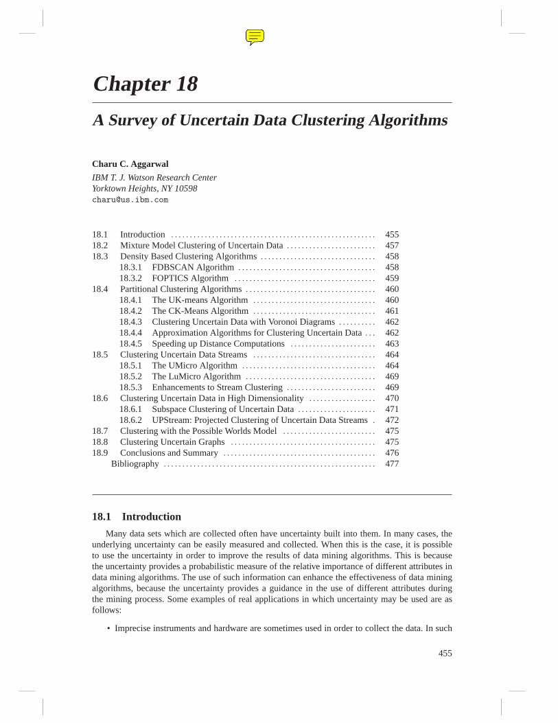
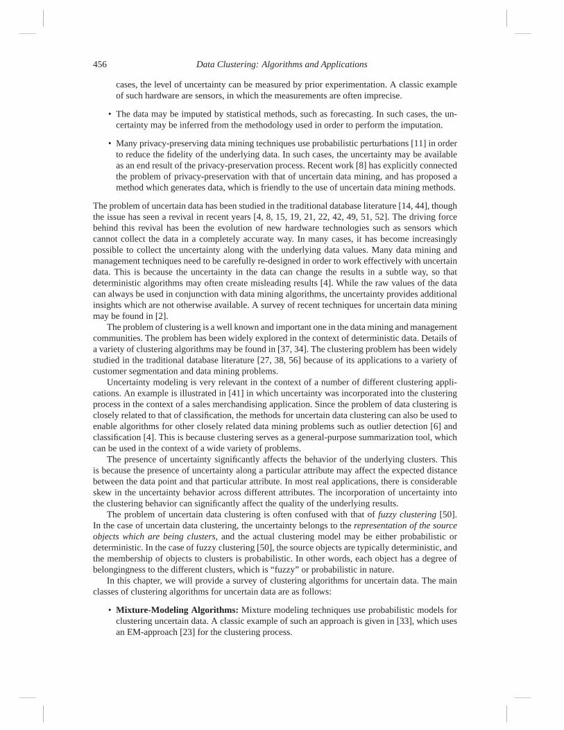
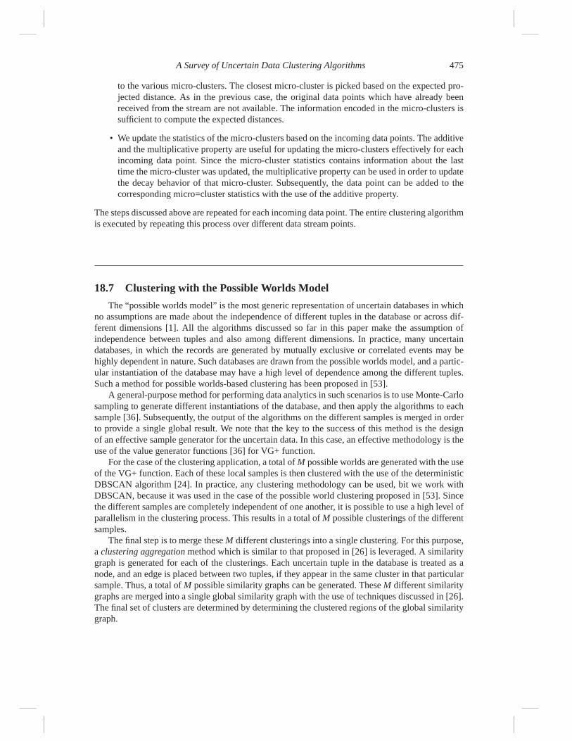
Density-based methods are very popular in the deterministic clustering literature, because oftheir ability to determine clusters of arbitrary shapes in the underlying data. The core-idea in thesemethods is to create a density profile of the data set with the use of kernel density estimation meth-ods. This density profile is then used in order to characterize the underlying clusters. In this section,we will discuss two variations of such density-based methods, which are the FDBSCAN and FOP-TICS methods.
18.3.1 FDBSCAN Algorithm
The presence of uncertainty changes the nature of the underlying clusters, since it affects thedistance function computations between different data points. A technique has been proposed in[42] in order to find density based clusters from uncertain data. The key idea in this approach is tocompute uncertain distances effectively between objects which are probabilistically specified. Thefuzzy distance is defined in terms of the distance distribution function. This distance distributionfunction encodes the probability that the distances between two uncertain objects lie within a certainuser-defined range. Let d(X ,Y ) be the random variable representing the distance between X and Y .The distance distribution function is formally defined as follows:
Definition 18.3.1 Let X and Y be two uncertain records, and let p(X ,Y ) represent the distancedensity function between these objects. Then, the probability that the distance lies within the range(a,b) is given by the following relationship:
P(a≤ d(X ,Y )≤ b) =∫ b
ap(X ,Y )(z)dz (18.1)
A Survey of Uncertain Data Clustering Algorithms 459
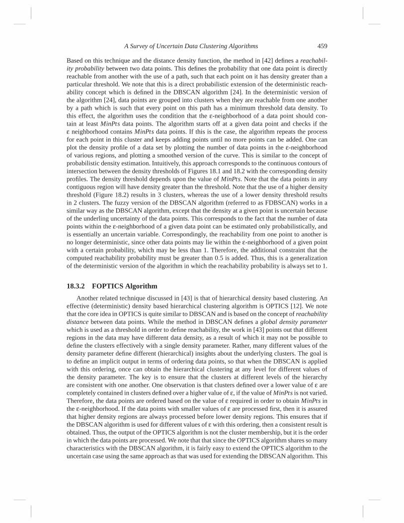
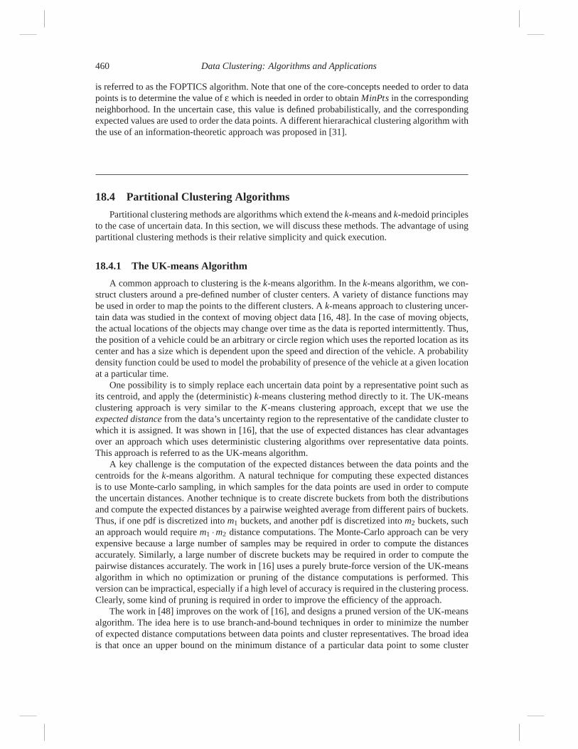
Based on this technique and the distance density function, the method in [42] defines a reachabil-ity probability between two data points. This defines the probability that one data point is directlyreachable from another with the use of a path, such that each point on it has density greater than aparticular threshold. We note that this is a direct probabilistic extension of the deterministic reach-ability concept which is defined in the DBSCAN algorithm [24]. In the deterministic version ofthe algorithm [24], data points are grouped into clusters when they are reachable from one anotherby a path which is such that every point on this path has a minimum threshold data density. Tothis effect, the algorithm uses the condition that the ε-neighborhood of a data point should con-tain at least MinPts data points. The algorithm starts off at a given data point and checks if theε neighborhood contains MinPts data points. If this is the case, the algorithm repeats the processfor each point in this cluster and keeps adding points until no more points can be added. One canplot the density profile of a data set by plotting the number of data points in the ε-neighborhoodof various regions, and plotting a smoothed version of the curve. This is similar to the concept ofprobabilistic density estimation. Intuitively, this approach corresponds to the continuous contours ofintersection between the density thresholds of Figures 18.1 and 18.2 with the corresponding densityprofiles. The density threshold depends upon the value of MinPts. Note that the data points in anycontiguous region will have density greater than the threshold. Note that the use of a higher densitythreshold (Figure 18.2) results in 3 clusters, whereas the use of a lower density threshold resultsin 2 clusters. The fuzzy version of the DBSCAN algorithm (referred to as FDBSCAN) works in asimilar way as the DBSCAN algorithm, except that the density at a given point is uncertain becauseof the underling uncertainty of the data points. This corresponds to the fact that the number of datapoints within the ε-neighborhood of a given data point can be estimated only probabilistically, andis essentially an uncertain variable. Correspondingly, the reachability from one point to another isno longer deterministic, since other data points may lie within the ε-neighborhood of a given pointwith a certain probability, which may be less than 1. Therefore, the additional constraint that thecomputed reachability probability must be greater than 0.5 is added. Thus, this is a generalizationof the deterministic version of the algorithm in which the reachability probability is always set to 1.
18.3.2 FOPTICS Algorithm
Another related technique discussed in [43] is that of hierarchical density based clustering. Aneffective (deterministic) density based hierarchical clustering algorithm is OPTICS [12]. We notethat the core idea in OPTICS is quite similar to DBSCAN and is based on the concept of reachabilitydistance between data points. While the method in DBSCAN defines a global density parameterwhich is used as a threshold in order to define reachability, the work in [43] points out that differentregions in the data may have different data density, as a result of which it may not be possible todefine the clusters effectively with a single density parameter. Rather, many different values of thedensity parameter define different (hierarchical) insights about the underlying clusters. The goal isto define an implicit output in terms of ordering data points, so that when the DBSCAN is appliedwith this ordering, once can obtain the hierarchical clustering at any level for different values ofthe density parameter. The key is to ensure that the clusters at different levels of the hierarchyare consistent with one another. One observation is that clusters defined over a lower value of ε arecompletely contained in clusters defined over a higher value of ε, if the value of MinPts is not varied.Therefore, the data points are ordered based on the value of ε required in order to obtain MinPts inthe ε-neighborhood. If the data points with smaller values of ε are processed first, then it is assuredthat higher density regions are always processed before lower density regions. This ensures that ifthe DBSCAN algorithm is used for different values of εwith this ordering, then a consistent result isobtained. Thus, the output of the OPTICS algorithm is not the cluster membership, but it is the orderin which the data points are processed. We note that that since the OPTICS algorithm shares so manycharacteristics with the DBSCAN algorithm, it is fairly easy to extend the OPTICS algorithm to theuncertain case using the same approach as that was used for extending the DBSCAN algorithm. This
460 Data Clustering: Algorithms and Applications
is referred to as the FOPTICS algorithm. Note that one of the core-concepts needed to order to datapoints is to determine the value of ε which is needed in order to obtain MinPts in the correspondingneighborhood. In the uncertain case, this value is defined probabilistically, and the correspondingexpected values are used to order the data points. A different hierarachical clustering algorithm withthe use of an information-theoretic approach was proposed in [31].
18.4 Partitional Clustering Algorithms
Partitional clustering methods are algorithms which extend the k-means and k-medoid principlesto the case of uncertain data. In this section, we will discuss these methods. The advantage of usingpartitional clustering methods is their relative simplicity and quick execution.
18.4.1 The UK-means Algorithm
A common approach to clustering is the k-means algorithm. In the k-means algorithm, we con-struct clusters around a pre-defined number of cluster centers. A variety of distance functions maybe used in order to map the points to the different clusters. A k-means approach to clustering uncer-tain data was studied in the context of moving object data [16, 48]. In the case of moving objects,the actual locations of the objects may change over time as the data is reported intermittently. Thus,the position of a vehicle could be an arbitrary or circle region which uses the reported location as itscenter and has a size which is dependent upon the speed and direction of the vehicle. A probabilitydensity function could be used to model the probability of presence of the vehicle at a given locationat a particular time.
One possibility is to simply replace each uncertain data point by a representative point such asits centroid, and apply the (deterministic) k-means clustering method directly to it. The UK-meansclustering approach is very similar to the K-means clustering approach, except that we use theexpected distance from the data’s uncertainty region to the representative of the candidate cluster towhich it is assigned. It was shown in [16], that the use of expected distances has clear advantagesover an approach which uses deterministic clustering algorithms over representative data points.This approach is referred to as the UK-means algorithm.
A key challenge is the computation of the expected distances between the data points and thecentroids for the k-means algorithm. A natural technique for computing these expected distancesis to use Monte-carlo sampling, in which samples for the data points are used in order to computethe uncertain distances. Another technique is to create discrete buckets from both the distributionsand compute the expected distances by a pairwise weighted average from different pairs of buckets.Thus, if one pdf is discretized into m1 buckets, and another pdf is discretized into m2 buckets, suchan approach would require m1 ·m2 distance computations. The Monte-Carlo approach can be veryexpensive because a large number of samples may be required in order to compute the distancesaccurately. Similarly, a large number of discrete buckets may be required in order to compute thepairwise distances accurately. The work in [16] uses a purely brute-force version of the UK-meansalgorithm in which no optimization or pruning of the distance computations is performed. Thisversion can be impractical, especially if a high level of accuracy is required in the clustering process.Clearly, some kind of pruning is required in order to improve the efficiency of the approach.
The work in [48] improves on the work of [16], and designs a pruned version of the UK-meansalgorithm. The idea here is to use branch-and-bound techniques in order to minimize the numberof expected distance computations between data points and cluster representatives. The broad ideais that once an upper bound on the minimum distance of a particular data point to some cluster
A Survey of Uncertain Data Clustering Algorithms 461
representative has been quantified, it is necessary to perform the computation between this pointand another cluster representative, if it can be proved that the corresponding distance is greater thanthis bound. In order to compute the bounds, the minimum bounding rectangle for the representativepoint for a cluster region is computed. The uncertain data point also represents a region over whichthe object may be distributed. For each representative cluster, its minimum bounding rectangle isused to compute the following two quantities with respect to the uncertain data point:
• The minimum limit on the expected distance between the MBR of the representative pointand the uncertain region for the data point itself.
• The maximum limit on the expected distance between the MBR of the representative pointand the uncertain region for the data point itself.
These upper and lower bound computations are facilitated by the use of the Minimum BoundingRectangles in conjunction with the triangle inequality. We note that a cluster representative can bepruned, if its maximum limit is less than the minimum limit for some other representative. Theapproach is [48] constructs a k-d tree on the cluster representatives in order to promote an orderlypruning strategy and minimize the number of representatives which need to be accessed. It wasshown in [48] that such an approach significantly improves the pruning efficiency over the bruteforce algorithm.
18.4.2 The CK-Means Algorithm
While the work in [16] claims that UK-means provides qualitatively superior results to deter-ministic clustering, the work in [45] shows that the model utilized by the UK-means is actuallyequivalent to deterministic clustering, by replacing each uncertain data point by its expected value.Thus, the UK-means approach actually turns out to be equivalent to deterministic clustering. Thiscontradicts the claim in [16] that the UK-means algorithm provides superior results to a determinis-tic clustering method which replaces uncertain data points with their centroids. We further note thatmost of the computational complexity is created by the running time required for expected distancecalculations. On the other hand, deterministic distance computations are extremely efficient, and arealmost always superior to any method which is based on expected distance computations, whetheror not pruning is used.
The UK-means algorithm aims to optimize the mean square expected distance about each clustercentroid. A key step is the computation of the expected square distance of an uncertain data pointXi with a cluster centroid Y , where the latter is approximated as a deterministic entity. Let Y be thecentroid of a cluster, and X1 . . .Xr be the set of data points in the cluster. Then, the expected meansquare distance of data point Xi about Y is given by E[||Xi−Y ||2]. Then, if Y is approximated as adeterministic entity, then we can show the following:
Lemma 18.4.1 Let Xi be an uncertain data point, and Y be a deterministic point. Let ci = E[Xi] andvar(Xi) represent the sum of the variances of the pdfs in Xi over all dimensions. Then, we have:
E[||Xi−Y ||2] = E[||Xi||2]−||ci||2 + ||ci−Y ||2= var(Xi)+ ||ci−Y ||2
We will provide a proof of a generalized version of this lemma slightly later (Lemma 18.4.2). Wefurther note that the value of E[||Xi||2]− ||ci||2 is equal to the variance of the uncertain data pointXi (summed over all dimensions). The term ||ci −Y ||2 is equal to the deterministic distance ofthe Y to the centroid of the uncertain data point Xi. Therefore, the expected square distance of anuncertain data point Xi to the centroid Y is given by the square sum of its deterministic distance and
462 Data Clustering: Algorithms and Applications
the variance of the data point Xi. The variance of the data point is not dependent on the value ofY . Therefore, while computing the expected square distance to the different centroids for the UK-means algorithm, it suffices to compute the deterministic distance to the centroid ci of Xi instead ofcomputing the expected square distance. This means that by replacing each uncertain data point Xi
with its centroid, the UK-means can be replicated exactly with an efficient deterministic algorithm.It is important to note that the equivalence of the UK-means method to a deterministic algo-
rithm is based on the approximation of treating each cluster centroid (in intermediate steps) as adeterministic entity. In practice, some of the dimensions may be much more uncertain than othersin the clustering process over most of the data points. This is especially the case when different di-mensions are collected using collection techniques with different fidelity. In such cases, the clustercentroids should not be treated as deterministic entities. Some of the streaming methods for uncer-tain data clustering such as those discussed in [5] also treat the cluster centroids as uncertain entitiesin order to enable more accurate computations. In those case, such deterministic approximations arenot possible. Another method, which treats cluster centroids as uncertain entities was later proposedindependently in [30]. The work on clustering streams, while treating centroids as uncertain entitieswill be discussed in a later section of this chapter.
18.4.3 Clustering Uncertain Data with Voronoi Diagrams
The work in [48] uses minimum bounding boxes of the uncertain objects in order to computedistance bounds for effective pruning. However, the use of minimax pruning can sometimes bequite restrictive in efficiently characterizing the uncertain object, which may have arbitrary shape.An approach which is based on voronoi diagrams, also improves the UK-means algorithms bycomputing the voronoi diagrams of the current set of cluster representatives [39]. Each cell in thisvoronoi diagram is associated with a cluster representative. We note that each cell in this voronoidiagram has the property that any point in this cell is closer to the cluster representative for that cell,than any other representative. Therefore, if the MBR of an uncertain object lies completely inside acell, then it is not necessary to compute its distance to any other cluster representatives. Similarly,for any pair of cluster representatives, the perpendicular bisector between the two is a hyperplanewhich is equidistant from the two representatives and is easily derivable from the voronoi diagram.In the event that the MBR of an uncertain object lies completely on one side of the bisector, we candeduce that one of the cluster representatives of closer to the uncertain object than the other. Thisallows us to prune of the representatives.
As in [48], this work is focused on pruning the number of expected distance computations. It hasbeen shown in [39] that the pruning power of the voronoi method is greater than the minmax methodproposed in [48]. However, the work in [39] does not compare its efficiency results to those in [45],which is based on the equivalence of UK-means to a deterministic algorithm, and does not requireany expected distance computations at all. It would seem to us, that any deterministic method fork-means clustering (as proposed in the reduction of [45]) should be much more efficient than amethod based on pruning the number of expected distance computations, no matter how effectivethe pruning methodology might be.
18.4.4 Approximation Algorithms for Clustering Uncertain Data
Recently, techniques have been designed for approximation algorithms for uncertain clusteringin [20]. The work in [20] discusses extensions of the k-mean and k-median version of the prob-lems. Bi-criteria algorithms are designed for each of these cases. One algorithm achieves a (1+ ε)-approximation to the best uncertain k-centers with the use of O(k ·ε−1 · log2(n)) centers. The secondalgorithm picks 2k centers and achieves a constant-factor approximation.
A key approach proposed in the paper [20] is the use of a transformation from the uncertaincase to a weighted version of the deterministic case. We note that solutions to the weighted version
A Survey of Uncertain Data Clustering Algorithms 463
of the deterministic clustering problem are well known, and require only a polynomial blow-up inthe problem size. The key assumption in solving the weighted deterministic case is that the ratioof the largest to smallest weights is polynomial. This assumption is assumed to be maintained inthe transformation. This approach can be used in order to solve both the uncertain k-means andk-median version of the problem with the afore-mentioned approximation guarantees. We refer thereader to [20, 28] for details of these algorithms.
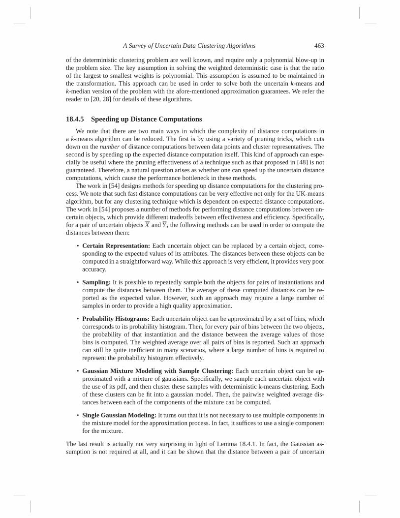
18.4.5 Speeding up Distance Computations
We note that there are two main ways in which the complexity of distance computations ina k-means algorithm can be reduced. The first is by using a variety of pruning tricks, which cutsdown on the number of distance computations between data points and cluster representatives. Thesecond is by speeding up the expected distance computation itself. This kind of approach can espe-cially be useful where the pruning effectiveness of a technique such as that proposed in [48] is notguaranteed. Therefore, a natural question arises as whether one can speed up the uncertain distancecomputations, which cause the performance bottleneck in these methods.
The work in [54] designs methods for speeding up distance computations for the clustering pro-cess. We note that such fast distance computations can be very effective not only for the UK-meansalgorithm, but for any clustering technique which is dependent on expected distance computations.The work in [54] proposes a number of methods for performing distance computations between un-certain objects, which provide different tradeoffs between effectiveness and efficiency. Specifically,for a pair of uncertain objects X and Y , the following methods can be used in order to compute thedistances between them:
• Certain Representation: Each uncertain object can be replaced by a certain object, corre-sponding to the expected values of its attributes. The distances between these objects can becomputed in a straightforward way. While this approach is very efficient, it provides very pooraccuracy.
• Sampling: It is possible to repeatedly sample both the objects for pairs of instantiations andcompute the distances between them. The average of these computed distances can be re-ported as the expected value. However, such an approach may require a large number ofsamples in order to provide a high quality approximation.
• Probability Histograms: Each uncertain object can be approximated by a set of bins, whichcorresponds to its probability histogram. Then, for every pair of bins between the two objects,the probability of that instantiation and the distance between the average values of thosebins is computed. The weighted average over all pairs of bins is reported. Such an approachcan still be quite inefficient in many scenarios, where a large number of bins is required torepresent the probability histogram effectively.
• Gaussian Mixture Modeling with Sample Clustering: Each uncertain object can be ap-proximated with a mixture of gaussians. Specifically, we sample each uncertain object withthe use of its pdf, and then cluster these samples with deterministic k-means clustering. Eachof these clusters can be fit into a gaussian model. Then, the pairwise weighted average dis-tances between each of the components of the mixture can be computed.
• Single Gaussian Modeling: It turns out that it is not necessary to use multiple components inthe mixture model for the approximation process. In fact, it suffices to use a single componentfor the mixture.
The last result is actually not very surprising in light of Lemma 18.4.1. In fact, the Gaussian as-sumption is not required at all, and it can be shown that the distance between a pair of uncertain
464 Data Clustering: Algorithms and Applications
objects (for which the pdfs are independent of one another), can be expressed purely as a functionof their means and variances. Therefore, we propose the following (slight) generalization of Lemma18.4.1.
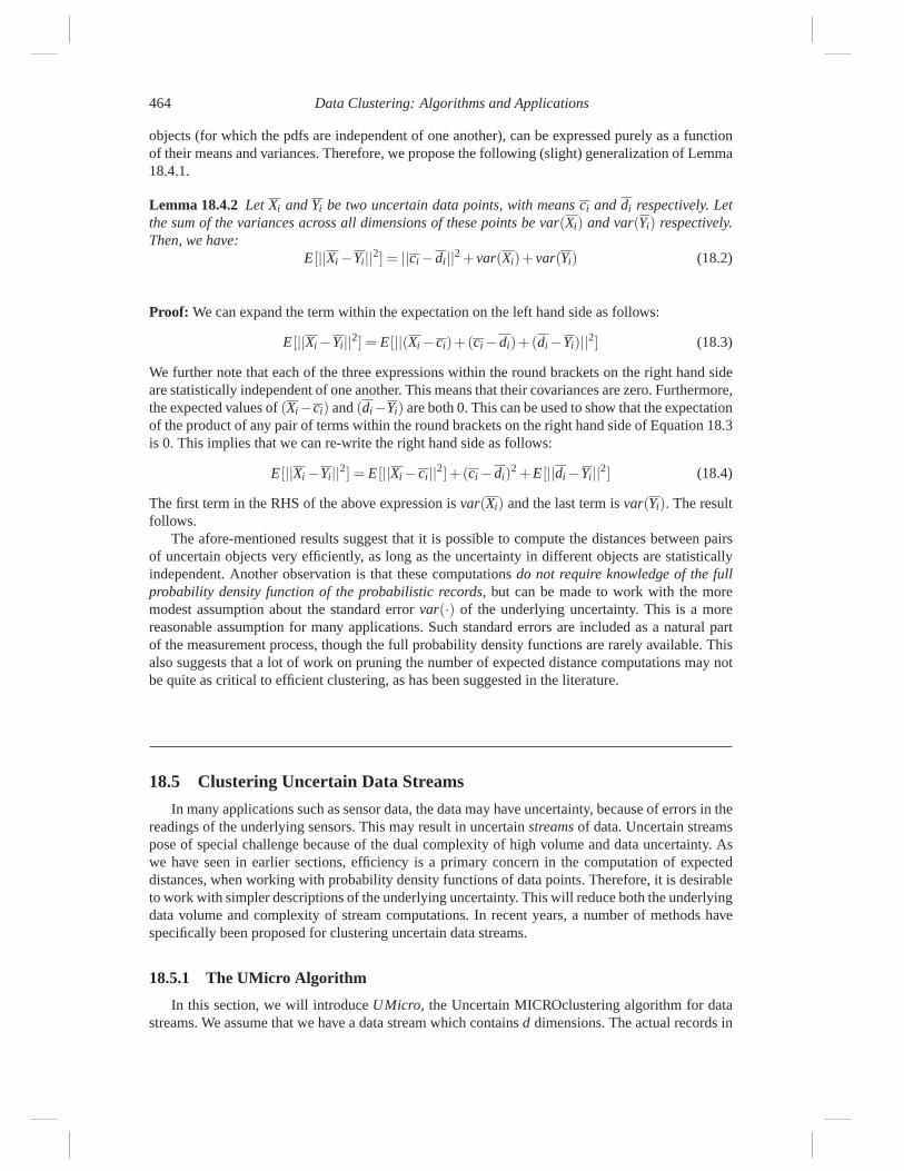
Lemma 18.4.2 Let Xi and Yi be two uncertain data points, with means ci and di respectively. Letthe sum of the variances across all dimensions of these points be var(Xi) and var(Yi) respectively.Then, we have:
E[||Xi−Yi||2] = ||ci−di||2 + var(Xi)+ var(Yi) (18.2)
Proof: We can expand the term within the expectation on the left hand side as follows:
E[||Xi−Yi||2] = E[||(Xi− ci)+(ci−di)+(di−Yi)||2] (18.3)
We further note that each of the three expressions within the round brackets on the right hand sideare statistically independent of one another. This means that their covariances are zero. Furthermore,the expected values of (Xi−ci) and (di−Yi) are both 0. This can be used to show that the expectationof the product of any pair of terms within the round brackets on the right hand side of Equation 18.3is 0. This implies that we can re-write the right hand side as follows:
E[||Xi−Yi||2] = E[||Xi− ci||2]+ (ci−di)2 +E[||di−Yi||2] (18.4)
The first term in the RHS of the above expression is var(Xi) and the last term is var(Yi). The resultfollows.
The afore-mentioned results suggest that it is possible to compute the distances between pairsof uncertain objects very efficiently, as long as the uncertainty in different objects are statisticallyindependent. Another observation is that these computations do not require knowledge of the fullprobability density function of the probabilistic records, but can be made to work with the moremodest assumption about the standard error var(·) of the underlying uncertainty. This is a morereasonable assumption for many applications. Such standard errors are included as a natural partof the measurement process, though the full probability density functions are rarely available. Thisalso suggests that a lot of work on pruning the number of expected distance computations may notbe quite as critical to efficient clustering, as has been suggested in the literature.
18.5 Clustering Uncertain Data Streams
In many applications such as sensor data, the data may have uncertainty, because of errors in thereadings of the underlying sensors. This may result in uncertain streams of data. Uncertain streamspose of special challenge because of the dual complexity of high volume and data uncertainty. Aswe have seen in earlier sections, efficiency is a primary concern in the computation of expecteddistances, when working with probability density functions of data points. Therefore, it is desirableto work with simpler descriptions of the underlying uncertainty. This will reduce both the underlyingdata volume and complexity of stream computations. In recent years, a number of methods havespecifically been proposed for clustering uncertain data streams.
18.5.1 The UMicro Algorithm
In this section, we will introduce UMicro, the Uncertain MICROclustering algorithm for datastreams. We assume that we have a data stream which contains d dimensions. The actual records in
A Survey of Uncertain Data Clustering Algorithms 465
the data are denoted by X1, X2, . . . XN . . .. We assume that the estimated error associated with thejth dimension for data point Xi is denoted by ψ j(Xi). This error is defined in terms of the standarddeviation of the error associated with the value of the jth dimension of Xi. The corresponding d-dimensional error vector is denoted by ψ(Xi). Thus, the input to the algorithm is a data stream in
which the ith pair is denoted by (Xi,ψ(Xi)).We note that most of the uncertain clustering techniques work with the assumption that the en-
tire probability density function is available. In many real applications, a more realistic assumptionis that only the standard deviations of the errors are available. This is because complete probabilitydistributions are rarely available, and are usually inserted only as a modeling assumption. An overlyambitious modeling assumption can also introduce modeling errors. It is also often quite natural tobe able to estimate the standard error in many modeling scenarios. For example, in a scientific ap-plication in which the measurements can vary from one observation to another, the error value is thestandard deviation of the observations over a large number of measurements. In a k-anonymity baseddata (or incomplete data) mining application, this is the standard deviation of the partially specified(or imputed) fields in the data. This is also more practical from a stream perspective, because itreduces the volume of the incoming stream, and reduces the complexity of stream computations.
The micro-clustering model was first proposed in [56] for large data sets, and subsequentlyadapted in [10] for the case of deterministic data streams. The UMicro algorithm extends the micro-clustering approach of [10] to the case of uncertain data. In order to incorporate the uncertainty intothe clustering process, we need a method to incorporate and leverage the error information into themicro-clustering statistics and algorithms. As discussed earlier, it is assumed that the data streamconsists of a set of multi-dimensional records X1 . . .Xk . . . arriving at time stamps T1 . . .Tk . . .. EachXi is a multi-dimensional record containing d dimensions which are denoted by Xi = (x1
i . . .xdi ). In
order to apply the micro-clustering method to the uncertain data mining problem, we need to alsodefine the concept of error-based micro-clusters. We define such micro-clusters as follows:
Definition 18.5.1 An uncertain micro-cluster for a set of d-dimensional points Xi1 . . .Xin with time
stamps Ti1 . . .Tin and error vectors ψ(Xi1) . . .ψ(Xin) is defined as the (3 · d + 2) tuple (CF2x(C ),EF2x(C ), CF1x(C ), t(C ), n(C )), wherein CF2x(C ), EF2x(C ), and CF1x(C ) each correspond to avector of d entries. The entries in EF2x(C ) correspond to the error-based entries. The definition ofeach of these entries is as follows:• For each dimension, the sum of the squares of the data values is maintained in CF2x(C ). Thus,
CF2x(C ) contains d values. The p-th entry of CF2x(C ) is equal to ∑nj=1(x
pi j)2. This corresponds to
the second moment of the data values along the p-th dimension.• For each dimension, the sum of the squares of the errors in the data values is maintained in
EF2x(C ). Thus, EF2x(C ) contains d values. The p-th entry of EF2x(C ) is equal to ∑nj=1ψp(Xi j)
2.This corresponds to the sum of squares of the errors in the records along the p-th dimension.• For each dimension, the sum of the data values is maintained in CF1x(C ). Thus, CF1x(C )
contains d values. The p-th entry of CF1x(C ) is equal to ∑nj=1 xp
i j. This corresponds to the first
moment of the values along the p-th dimension.• The number of points in the data is maintained in n(C ).• The time stamp of the last update to the micro-cluster is maintained in t(C ).
We note that the uncertain definition of micro-clusters differs from the deterministic definition, sincewe have added an additional d values corresponding to the error information in the records. We willrefer to the uncertain micro-cluster for a set of points C by ECF(C ). We note that error based micro-clusters maintain the important additive property [10] which is critical to its use in the clusteringprocess. We restate the additive property as follows:
Property 18.5.1 Let C1 and C2 be two sets of points. Then all non-temporal components of theerror-based cluster feature vector ECF(C1∪C2) are given by the sum of ECF(C1) and ECF(C2).
466 Data Clustering: Algorithms and Applications
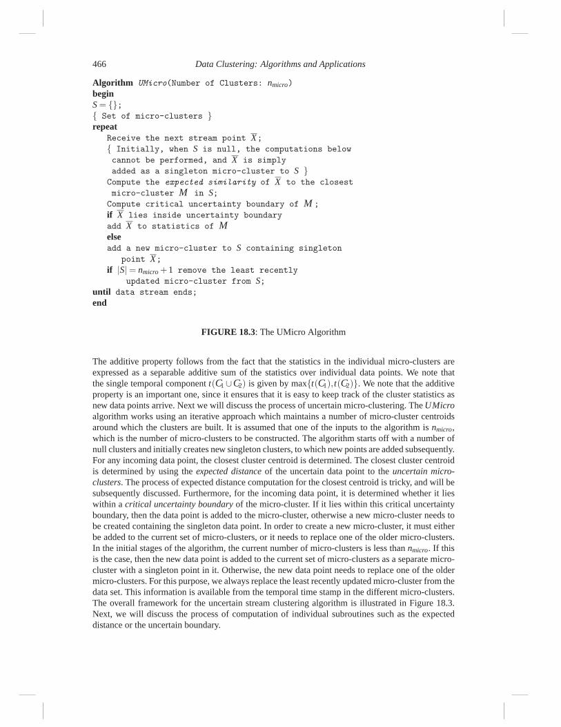
Algorithm UMicro(Number of Clusters: nmicro)
beginS = {};{ Set of micro-clusters }repeat
Receive the next stream point X;{ Initially, when S is null, the computations below
cannot be performed, and X is simply
added as a singleton micro-cluster to S }Compute the expected similarity of X to the closest
micro-cluster M in S;Compute critical uncertainty boundary of M ;
if X lies inside uncertainty boundary
add X to statistics of Melseadd a new micro-cluster to S containing singleton
point X;if |S|= nmicro +1 remove the least recently
updated micro-cluster from S;until data stream ends;
end
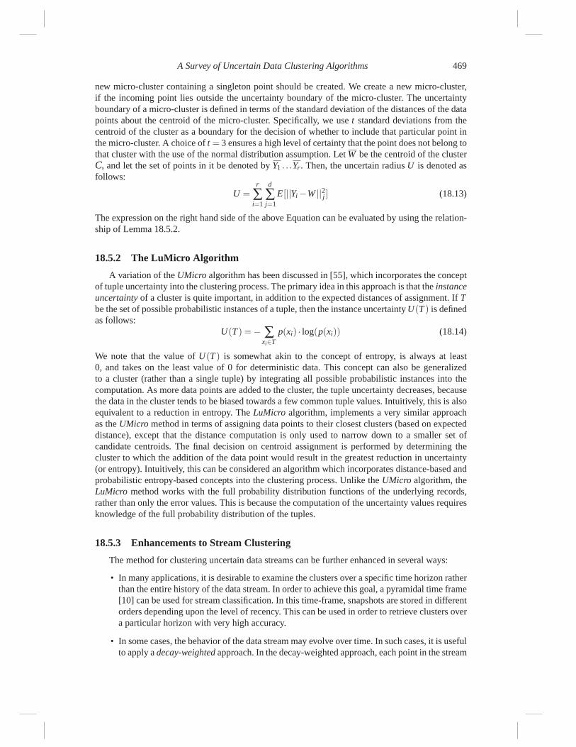
FIGURE 18.3: The UMicro Algorithm
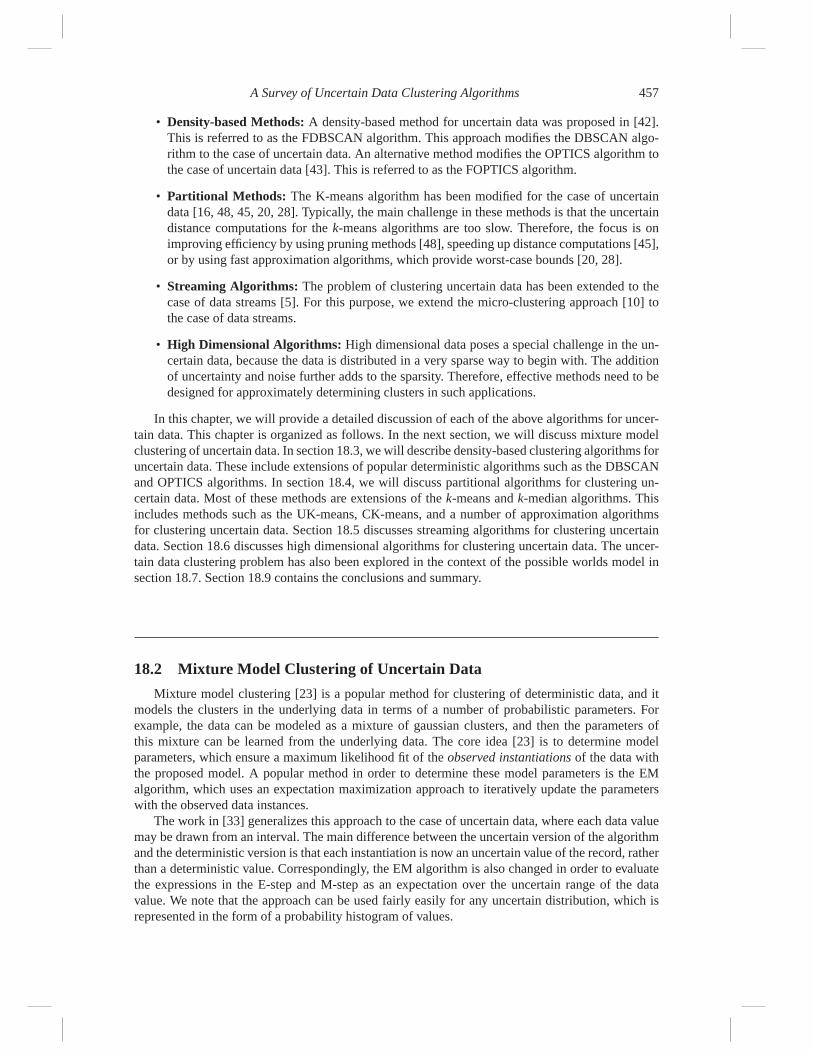
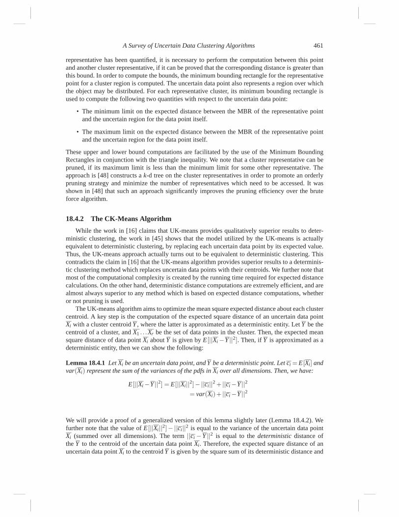
The additive property follows from the fact that the statistics in the individual micro-clusters areexpressed as a separable additive sum of the statistics over individual data points. We note thatthe single temporal component t(C1∪C2) is given by max{t(C1), t(C2)}. We note that the additiveproperty is an important one, since it ensures that it is easy to keep track of the cluster statistics asnew data points arrive. Next we will discuss the process of uncertain micro-clustering. The UMicroalgorithm works using an iterative approach which maintains a number of micro-cluster centroidsaround which the clusters are built. It is assumed that one of the inputs to the algorithm is nmicro,which is the number of micro-clusters to be constructed. The algorithm starts off with a number ofnull clusters and initially creates new singleton clusters, to which new points are added subsequently.For any incoming data point, the closest cluster centroid is determined. The closest cluster centroidis determined by using the expected distance of the uncertain data point to the uncertain micro-clusters. The process of expected distance computation for the closest centroid is tricky, and will besubsequently discussed. Furthermore, for the incoming data point, it is determined whether it lieswithin a critical uncertainty boundary of the micro-cluster. If it lies within this critical uncertaintyboundary, then the data point is added to the micro-cluster, otherwise a new micro-cluster needs tobe created containing the singleton data point. In order to create a new micro-cluster, it must eitherbe added to the current set of micro-clusters, or it needs to replace one of the older micro-clusters.In the initial stages of the algorithm, the current number of micro-clusters is less than nmicro. If thisis the case, then the new data point is added to the current set of micro-clusters as a separate micro-cluster with a singleton point in it. Otherwise, the new data point needs to replace one of the oldermicro-clusters. For this purpose, we always replace the least recently updated micro-cluster from thedata set. This information is available from the temporal time stamp in the different micro-clusters.The overall framework for the uncertain stream clustering algorithm is illustrated in Figure 18.3.Next, we will discuss the process of computation of individual subroutines such as the expecteddistance or the uncertain boundary.
A Survey of Uncertain Data Clustering Algorithms 467
In order to compute the expected similarity of the data point X to the centroid of the cluster C ,we need to determine a closed form expression which is expressed only in terms of X and ECF(C ).We note that just as the individual data points are essential random variables with a given error, thecentroid Z of a cluster C is also a random variable. We make the following observation about thecentroid of a cluster:
Lemma 18.5.1 Let Z be the random variable representing the centroid of cluster C . Then, thefollowing result holds true:
E[||Z||2] =d
∑j=1
CF1(C )2j/n(C )2 +
d
∑j=1
EF2(C ) j/n(C )2 (18.5)
Proof: We note that the random variable Zj is given by the current instantiation of the centroid andthe mean of n(C ) different error terms for the points in cluster C . Therefore, we have:
Z j =CF1(C ) j/n(C )+ ∑X∈C
e j(X)/n(C ) (18.6)
Then, by squaring Zj and taking the expected value, we obtain the following:
E[Z2j ] =CF1(C )2
j/n(C )2 +2 · ∑X∈C
E[e j(X)] ·CF1(C ) j/n(C )2 +E[(∑X∈C
e j(X))2]/n(C )2 (18.7)
Now, we note that the error term is a random variable with standard deviation ψ j(·) and zero mean.Therefore E[e j] = 0. Further, since it is assumed that the random variables corresponding to theerrors of different records are independent of one another, we have E[e j(X) · e j(Y )] = E[e j(X)] ·E[e j(Y )] = 0. By using these relationships in the expansion of the above equation we get:
E[Z2j ] =CF1(C )2
j/n(C )2 + ∑X∈C
E[e j(X)2]/n(C )2 =CF1(C )2j/n(C )2 + ∑
X∈Cψ j(X)2/n(C )2
=CF1(C )2j/n(C )2 +EF2(C ) j/n(C )2
By adding the value of E[Z2j ] over different values of j, we get:
E[||Z||2] =d
∑j=1
CF1(C )2j/n(C )2 +
d
∑j=1
EF2(C ) j/n(C )2 (18.8)
This proves the desired result.Next, we will use the above result to directly estimate the expected distance between the centroid
of cluster C and the data point X . We will prove the following result:
Lemma 18.5.2 Let v denote the expected value of the square of the distance between the uncertaindata point X = (x1 . . .xd) (with instantiation (x1 . . .xd) and error vector (ψ1(X) . . .ψd(X)) and thecentroid of cluster C . Then, v is given by the following expression:
v =d
∑j=1
CF1(C )2j/n(C )2 +
d
∑j=1
EF2(C ) j/n(C )2 +d
∑j=1
x2j +
d
∑j=1
(ψ j(X))2−2d
∑j=1
x j ·CF1(C ) j/n(C )
(18.9)
468 Data Clustering: Algorithms and Applications
Proof: Let Z represent the centroid of cluster C . Then, we have:
v = E[||X−Z||2] = E[||X ||2]+E[||Z||2]−2E[X ·Z] = E[||X ||2]+E[||Z||2]−2E[X ] ·E[Z]
Next, we will analyze the individual terms in the above expression. We note that the value of X is arandom variable, whose expected value is equal to its current instantiation, and it has an error alongthe jth dimension which is equal to ψ j(X). Therefore, the expected value of E[||X ||2] is given by:
E[||X ||2] = (E[X ])2 +d
∑j=1
(ψ j(X))2 =d
∑j=1
x2j +
d
∑j=1
(ψ j(X))2
Now, we note that the jth term of E[Z] is equal to the jth dimension of the centroid of cluster C . Thisis given by the expression CF1(C ) j/n(C ), where CF1 j(C ) is the jth term of the first order clustercomponent CF1(C ). Therefore, the value of E[X ] ·E[Z] is given by the following expression:
E[X ] ·E[Z] =d
∑j=1
x j ·CF1(C ) j/n(C ) (18.10)
The results above and Lemma 18.5.1 define the values of E[||X ||2], E[||Z||2], and E[X ·Z]. Note thatall of these values occur in the right hand side of the following relationship:
v = E[||X ||2]+E[||Z||2]−2E[X ] ·E[Z] (18.11)
By substituting the corresponding values in the right hand side of the above relationship, we get:
v =d
∑j=1
CF1(C )2j/n(C )2 +
d
∑j=1
EF2(C ) j/n(C )2 +d
∑j=1
x2j +
d
∑j=1
(ψ j(X))2−2d
∑j=1
x j ·CF1(C ) j/n(C )
(18.12)The result follows.
The result of Lemma 18.5.2 establishes how the square of the distance may be computed (inexpected value) using the error information in the data point X and the micro-cluster statistics of C .Note that this is an efficient computation which requires O(d) operations, which is asymptoticallythe same as the deterministic case. This is important since distance function computation is themost repetitive of all operations in the clustering algorithm, and we would want it to be as efficientas possible.
While the expected distances can be directly used as a distance function, the uncertainty addsa lot of noise to the computation. We would like to remove as much noise as possible in order todetermine the most accurate clusters. Therefore, we design a dimension counting similarity functionwhich prunes the uncertain dimensions during the similarity calculations. This is done by computingthe variance σ2
j along each dimension j. The computation of the variance can be done by using thecluster feature statistics of the different micro-clusters. The cluster feature statistics of all micro-clusters are added to create one global cluster feature vector. The variance of the data points alongeach dimension can then be computed from this vector by using the method discussed in [56].For each dimension j and threshold value thresh, we add the similarity value max{0,1−E[||X −Z||2j ]/(thresh∗σ2
j)} to the computation. We note that this is a similarity value rather than a distancevalue, since larger values imply greater similarity. Furthermore, dimensions which have a largeamount of uncertainty are also likely to have greater values of E[||X −Z||2j ], and are often prunedfrom the computation. This improves the quality of the similarity computation.
In this section, we will describe the process of computing the uncertain boundary of a micro-cluster. Once the closest micro-cluster for an incoming point has been determined, we need todecide whether it should be added to the corresponding micro-clustering statistics, or whether a
A Survey of Uncertain Data Clustering Algorithms 469
new micro-cluster containing a singleton point should be created. We create a new micro-cluster,if the incoming point lies outside the uncertainty boundary of the micro-cluster. The uncertaintyboundary of a micro-cluster is defined in terms of the standard deviation of the distances of the datapoints about the centroid of the micro-cluster. Specifically, we use t standard deviations from thecentroid of the cluster as a boundary for the decision of whether to include that particular point inthe micro-cluster. A choice of t = 3 ensures a high level of certainty that the point does not belong tothat cluster with the use of the normal distribution assumption. Let W be the centroid of the clusterC , and let the set of points in it be denoted by Y1 . . .Yr. Then, the uncertain radius U is denoted asfollows:
U =r
∑i=1
d
∑j=1
E[||Yi−W ||2j ] (18.13)
The expression on the right hand side of the above Equation can be evaluated by using the relation-ship of Lemma 18.5.2.
18.5.2 The LuMicro Algorithm
A variation of the UMicro algorithm has been discussed in [55], which incorporates the conceptof tuple uncertainty into the clustering process. The primary idea in this approach is that the instanceuncertainty of a cluster is quite important, in addition to the expected distances of assignment. If Tbe the set of possible probabilistic instances of a tuple, then the instance uncertainty U(T ) is definedas follows:
U(T ) =− ∑xi∈T
p(xi) · log(p(xi)) (18.14)
We note that the value of U(T ) is somewhat akin to the concept of entropy, is always at least0, and takes on the least value of 0 for deterministic data. This concept can also be generalizedto a cluster (rather than a single tuple) by integrating all possible probabilistic instances into thecomputation. As more data points are added to the cluster, the tuple uncertainty decreases, becausethe data in the cluster tends to be biased towards a few common tuple values. Intuitively, this is alsoequivalent to a reduction in entropy. The LuMicro algorithm, implements a very similar approachas the UMicro method in terms of assigning data points to their closest clusters (based on expecteddistance), except that the distance computation is only used to narrow down to a smaller set ofcandidate centroids. The final decision on centroid assignment is performed by determining thecluster to which the addition of the data point would result in the greatest reduction in uncertainty(or entropy). Intuitively, this can be considered an algorithm which incorporates distance-based andprobabilistic entropy-based concepts into the clustering process. Unlike the UMicro algorithm, theLuMicro method works with the full probability distribution functions of the underlying records,rather than only the error values. This is because the computation of the uncertainty values requiresknowledge of the full probability distribution of the tuples.
18.5.3 Enhancements to Stream Clustering
The method for clustering uncertain data streams can be further enhanced in several ways:
• In many applications, it is desirable to examine the clusters over a specific time horizon ratherthan the entire history of the data stream. In order to achieve this goal, a pyramidal time frame[10] can be used for stream classification. In this time-frame, snapshots are stored in differentorders depending upon the level of recency. This can be used in order to retrieve clusters overa particular horizon with very high accuracy.
• In some cases, the behavior of the data stream may evolve over time. In such cases, it is usefulto apply a decay-weighted approach. In the decay-weighted approach, each point in the stream
470 Data Clustering: Algorithms and Applications
X
X
X
X
X
X
X
X
POINT SET A
POINT SET B
X−AXIS
Y−AXIS
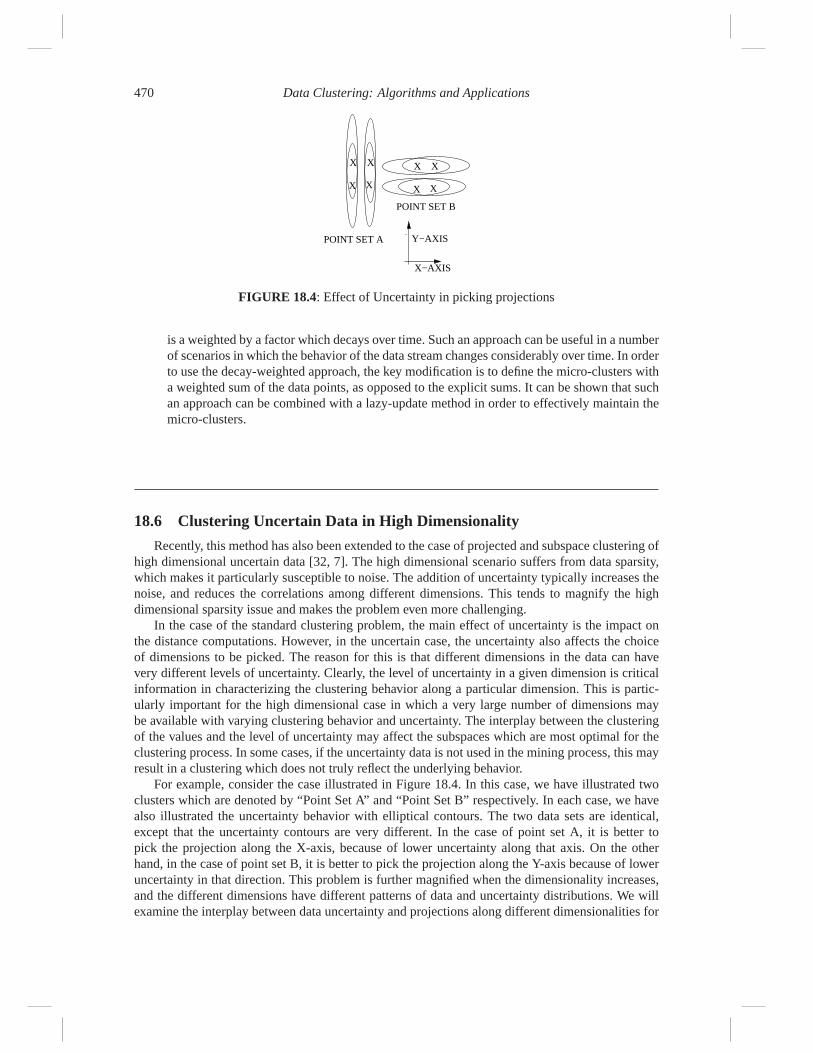
FIGURE 18.4: Effect of Uncertainty in picking projections
is a weighted by a factor which decays over time. Such an approach can be useful in a numberof scenarios in which the behavior of the data stream changes considerably over time. In orderto use the decay-weighted approach, the key modification is to define the micro-clusters witha weighted sum of the data points, as opposed to the explicit sums. It can be shown that suchan approach can be combined with a lazy-update method in order to effectively maintain themicro-clusters.
18.6 Clustering Uncertain Data in High Dimensionality
Recently, this method has also been extended to the case of projected and subspace clustering ofhigh dimensional uncertain data [32, 7]. The high dimensional scenario suffers from data sparsity,which makes it particularly susceptible to noise. The addition of uncertainty typically increases thenoise, and reduces the correlations among different dimensions. This tends to magnify the highdimensional sparsity issue and makes the problem even more challenging.
In the case of the standard clustering problem, the main effect of uncertainty is the impact onthe distance computations. However, in the uncertain case, the uncertainty also affects the choiceof dimensions to be picked. The reason for this is that different dimensions in the data can havevery different levels of uncertainty. Clearly, the level of uncertainty in a given dimension is criticalinformation in characterizing the clustering behavior along a particular dimension. This is partic-ularly important for the high dimensional case in which a very large number of dimensions maybe available with varying clustering behavior and uncertainty. The interplay between the clusteringof the values and the level of uncertainty may affect the subspaces which are most optimal for theclustering process. In some cases, if the uncertainty data is not used in the mining process, this mayresult in a clustering which does not truly reflect the underlying behavior.
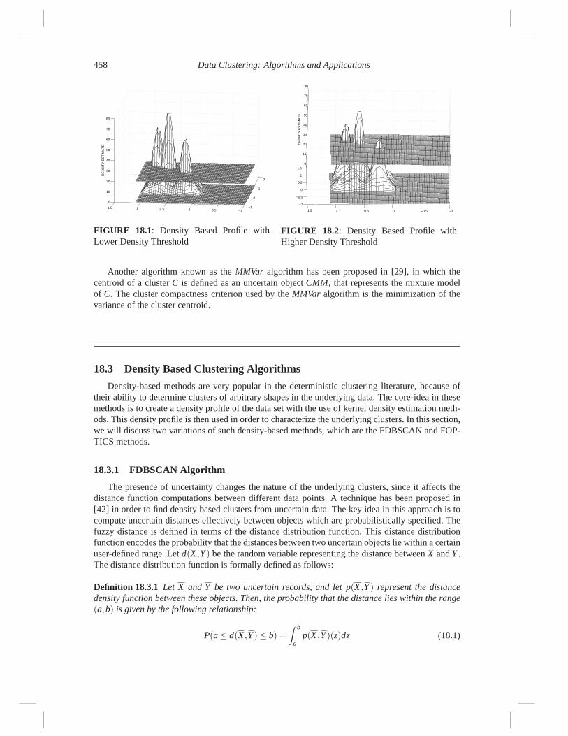
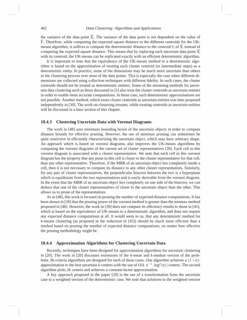
For example, consider the case illustrated in Figure 18.4. In this case, we have illustrated twoclusters which are denoted by “Point Set A” and “Point Set B” respectively. In each case, we havealso illustrated the uncertainty behavior with elliptical contours. The two data sets are identical,except that the uncertainty contours are very different. In the case of point set A, it is better topick the projection along the X-axis, because of lower uncertainty along that axis. On the otherhand, in the case of point set B, it is better to pick the projection along the Y-axis because of loweruncertainty in that direction. This problem is further magnified when the dimensionality increases,and the different dimensions have different patterns of data and uncertainty distributions. We willexamine the interplay between data uncertainty and projections along different dimensionalities for
A Survey of Uncertain Data Clustering Algorithms 471
the clustering process. We will show that the incorporation of uncertainty information into criticalalgorithmic decisions leads to much better quality of the clustering.
In this section, we will discuss two different algorithms, one of which allows overlap among thedifferent clusters, and the other designs a method for strict partitioning of the data in the uncertainstreaming scenario. The first case creates a soft partitioning of the data, in which data points belongto clusters with a probability. This is also referred to as membership degree, a concept which wewill discuss in the next subsection.
18.6.1 Subspace Clustering of Uncertain Data
A subspace clustering algorithm for uncertain data was proposed in [32]. The algorithm usesa grid based method, which attempts to search on the space of medoids and subspaces for theclustering process. In the grid-based approach, the support is counted with a width w on the relevantsubset of dimensions. Thus, for a given medoid m, we examine a distance w from the medoid alongeach of the relevant dimensions. The support of the hypercubes of this grid provide us with anidea of the dense subspaces in the data. For the other dimensions, unlimited width is considered.A Monte-Carlo sampling approach is used in order to search on the space of possible medoids.The core unit of the algorithm is a Monte-Carlo sampling approach, which generates a single goodsubspace cluster from the database.
In order to achieve this goal, a total of numMedoids are sampled from the underlying data. Foreach such medoid, its best possible local subspace is constructed, in order to generate the grid-basedsubspace cluster. The quality of this local subspace is identified, and the best medoid (and associatedsubspace cluster) among all the numMedoids different possibilities is identified. In order to generatethe local subspaces around the medoid, a support parameter called minSup is used. For all localsubspaces (corresponding to grid width w), which have support of at least minSup, the quality of thecorresponding subspace is determined. The quality of a local subspace cluster is different from thesupport in order to account for the different number of dimensions in the different subspaces. If thisquality is the best encountered so far, then we update the best medoid (and corresponding subspace)encountered so far. The quality function for a medoid m and subspace S is related to the support asfollows:
quality(m,S) = support(m,S)∗1/β|S| (18.15)
Here β ∈ (0,1) normalizes for the different number of dimensions in the different subspaces S. Theidea is that a subspace with a larger number of dimensions, but with the same support, is consideredto be of better quality. A number of different methods can be used in order to compute the supportof the subset S of dimensions:
• Expectation-based Support: In this case, the support is defined as the number of data points,whose centroids lie within a given distance w of the medoid along the relevant dimensions.Essentially, this method for support computation is similar to the deterministic case by re-placing uncertain objects with their centroids.
• Minimal Probability-based Support: In this case, the support is defined as the number ofdata points, which have a minimum probability of being within a distance of w from themedoid along each of the relevant dimensions.
• Exact Probability-based Support: This computes the sum of the probabilities that the dif-ferent objects lie within a distance of w along each of the relevant dimensions. This value isactually equal to expected number of objects which lie within a width of w along the relevantdimensions.
We note that the last two measurements require the computation of a probability that an uncertain
472 Data Clustering: Algorithms and Applications
object lies within a specific width w of a medoid. This probability also reflects the membershipdegree of the data point to the cluster.
We note that the afore-mentioned technique only generates a single subspace cluster with theuse of sampling. A question arises as to how we can generalize this in order to generate the overallclustering. We note that repeated samplings may generate the same set of clusters, a scenario whichwe wish to avoid. In order to reduce repeated clusters, two approaches can be used:
• Objects which have a minimal probability of belonging to any of the previously generatedclusters are excluded from consideration for being medoids.
• The probability of an object being selected as a medoid depends upon its membership degreeto the previously generated clusters. Objects which have very low membership degrees topreviously generated clusters have a higher probability of being selected as medoids.
The work in [32] explores the different variations of the subspace clustering algorithms, and showsthat the methods are superior to methods such as UK-means and deterministic projected clusteringalgorithms such as PROCLUS [3].
18.6.2 UPStream: Projected Clustering of Uncertain Data Streams
The UPStream algorithm is designed for the high dimensional uncertain stream scenario. Thisalgorithm can be considered an extension of the UMicro algorithm. The error model of the UP-Stream algorithm is quite different from the algorithm of [32], and uses a model of error standarddeviations rather than the entire probability distribution. This model is more similar to the UMicroalgorithm.
The data stream consists of a set of incoming records which are denoted by X1 . . .Xi . . .. It isassumed that the data point Xi is received at the time stamp Ti. It is assumed that the dimensionalityof the data set is d. The d dimensions of the record Xi are denoted by (x1
i . . .xdi ). In addition, each
data point has an error associated with the different dimensions. The error (standard-deviation)associated with the jth dimension for data point Xi is denoted by ψ j(Xi).
In order to incorporate the greater importance of recent data points in an evolving stream, we usethe concept of a fading function f (t), which quantifies the relative importance of the different datapoints over time. The fading function is drawn from the range (0,1), and serves as a multiplicativefactor for the relative importance of a given data point. This function is a monotonically decreasingfunction, and represents the gradual fading of importance of a data point over time. A commonlyused decay function is the exponential decay function. This function is defined as follows. Theexponential decay-function f (t) with parameter λ is defined as follows as a function of the time t:
f (t) = 2−λ·t (18.16)
We note that the value of f (t) reduces by a factor of 2 every 1/λ time units. This corresponds to thehalf-life of the function f (t). We define the half-life as follows:
Definition 18.6.1 The half-life of the function f (·) is defined as the time t at which f (t) = (1/2) ·f (0). For the exponential decay function, the half-life is 1/λ.
In order to keep track of the statistics for cluster creation, two sets of statistics are maintained:
• Global data statistics which keep track of the variance along different dimensions of the data.This data is necessary in order to maintain information about the scaling behavior of theunderlying data.
• Fading micro-cluster statistics which keep track of the cluster behavior, the projection dimen-sions as well as the underlying uncertainty.
A Survey of Uncertain Data Clustering Algorithms 473
Let us assume that the data points that have arrived so far are X1 . . .XN . . .. Let tc be the current time.
• For each dimension, the weighted sum of the squares of the individual dimensions ofX1 . . .XN . . . over the entire data stream are maintained. There are a total of d such entries.The ith component of the global second-order statistics is denoted by gs(i) and is equal to∑N
j=1 f (tc−Tj) · (xij)
2.
• For each dimension, the sum of the individual dimensions of X1 . . .XN . . . over the entire datastream are maintained. There are a total of d such entries. The ith component of the globalfirst-order statistics is denoted by g f (i) and is equal to ∑N
j=1 f (tc−Tj) · (xij).
• The sum of the weights of the different values of f (Tj) are maintained. This value is equal to∑N
j=1 f (tc−Tj). This value is denoted by gW .
The above statistics can be easily maintained over a data stream since the values are computedadditively over arriving data points. At first sight, it would seem that the statistics need to be updatedat each clock tick. In reality, because of the multiplicative nature of the exponential distribution, weonly need to update the statistics on the arrival of each new data point. Whenever a new data pointarrives at time Ti, we multiply each of the statistics by e−λ·Ti−Ti−1 and then add the statistics for theincoming data point Xi. We note that the global variance along a given dimension can be computedfrom the above values. Therefore, the global variance can be maintained continuously over the entiredata stream.
Observation 18.6.1 The variance along the ith dimension is given by gs(i)gW − g f (i)2
gW 2 .
The above fact can be easily proved by using the fact that for any random variable Y the variancevar(Y ) is given by E[Y 2]−E[Y ]2. We will denote the global standard deviation along dimension iat time tc by σ(i, tc). As suggested by the observation above, the value of σ(i, tc) is easy to maintainby using the global statistics discussed above.
An uncertain micro-cluster C = {Xi1 . . .XiN} is represented as follows.
Definition 18.6.2 The uncertain micro-cluster for a set of d-dimensional points Xi1 . . .Xin with time
stamps given by Ti1 . . .Tin , and error vectors ψ(Xi1) . . .ψ(Xin) is defined as the (3 · d + 3) tupleECF(C ) = (CF2(C ),EF2(C ), CF1(C ), t(C ),W (C ),n(C )), and a d-dimensional bit vector B(C ),wherein the corresponding entries are defined as follows:
• For each of the d dimensions, we maintain the weighted sum of the squares of the data valuesin CF2(C ). The p-th entry is given by ∑n
j=1 f (t−Ti j) · (xpi j)2.
• For each of the d dimensions, we maintain the weighted sum of the squares of the errors (alongthe corresponding dimension) in EF2(C ). The p-th entry is given by∑n
j=1 f (t−Ti j) ·ψp(Xi j)2.
• For each of the d dimensions, we maintain the weighted sum of the data values in CF1(C ).The p-th entry is given by ∑n
j=1 f (t−Ti j) · xpi j
.
• The sum of the weights is maintained in W (C ). This value is equal to ∑nj=1 f (t−Ti j).
• The number of data points is maintained in n(C ).
• The last time at which a data point was added to the cluster is maintained in t(C ).
• We also maintain a d-dimensional bit-vector B(C ). Each bit in this vector corresponds to adimension. A bit in this vector takes on the value of 1, if that dimension is included in theprojected cluster. Otherwise, the value of the bit is zero.
474 Data Clustering: Algorithms and Applications
This definition is quite similar to the case of the UMicro algorithm, except that there is also afocus on maintaining dimension-specific information and the time-decay information. We note thatthe micro-cluster definition discussed above satisfies two properties: the additive property, and themultiplicative property. The additive property is common to all micro-clustering techniques:
Observation 18.6.2 Additive Property Let C1 and C2 be two sets of points. Then the componentsof the error-based cluster feature vector (other than the time stamp) ECF(C1∪C2) are given by thesum of ECF(C1) and ECF(C2).
The additive property is helpful in streaming applications, since the statistics for the micro-clusterscan be modified by simply adding the statistics for the incoming data points to the micro-clusterstatistics. However, the micro-cluster statistics also include time-decay information of the underly-ing data points, which can potentially change at each time-stamp. Therefore, we need an effectiveway to update the micro-cluster statistics without having to explicitly do so at each time stamp. Forthis purpose, the multiplicative-property is useful.
Observation 18.6.3 Multiplicative Property The decaying components of ECF(C ) at time tc canbe obtained from the component values at time ts < tc by multiplying each component by 2−λ·(tc−ts)
provided that no new points have been added to a micro-cluster.
The multiplicative property follows from the fact the statistics decay at the multiplicative rate of2−λ at each tick. We note that the multiplicative-property is important in ensuring that a lazy updateprocess can be used for updating the decaying micro-clusters, rather than at each clock-tick. In thelazy-update process, we update a micro-cluster only when a new data point is added to it. In order todo so, we first use the multiplicative property to adjust for time-decay, and then we use the additiveproperty to add the incoming point to the micro-cluster statistics.
The UPStream algorithm uses a continuous partitioning and projection strategy in which thedifferent micro-clusters in the stream are associated with a particular projection, and this projectionis used in order to define the assignment of data points to clusters. The input to the algorithm is thenumber of micro-clusters k which are to be determined by the algorithm. The algorithm starts offwith a empty set of clusters. The initial set of k data points are assigned to singleton clusters in orderto create the initial set of seed micro-clusters. This initial set of micro-cluster statistics provides astarting point which is rapidly modified by further updates to the micro-clusters. For each incomingdata point, probabilistic measures are computed over the projected dimensions in order to determinethe assignment of data points to clusters. These assignments are used to update the statistics of theunderlying clusters. These updates are combined with a probabilistic approach for determining theexpected distances and spreads along the projected dimensions. In each update iteration, the detailsof the steps performed are as follows:
• We compute the global moment statistics associated with the data stream by using the multi-plicative and additive property. If ts be the last time of arrival of a data stream point, and tc bethe current time of arrival, then we multiply the moment statistics by 2−λ·(tc−ts), and add thecurrent data point.
• For each micro-cluster, we compute and update the set of dimensions associated with it. Thiscomputation process uses both the uncertainty information of data points within the differentmicro-clusters. A critical point here is that the original data points which have already beenreceived from the stream are not available, but only the summary micro-cluster information isavailable. The results in [7] show that the summary information encoded in the micro-clustersis sufficient to determine the projected dimensions effectively.
• We use the projected dimensions in order to compute the expected distances of the data points
A Survey of Uncertain Data Clustering Algorithms 475
to the various micro-clusters. The closest micro-cluster is picked based on the expected pro-jected distance. As in the previous case, the original data points which have already beenreceived from the stream are not available. The information encoded in the micro-clusters issufficient to compute the expected distances.
• We update the statistics of the micro-clusters based on the incoming data points. The additiveand the multiplicative property are useful for updating the micro-clusters effectively for eachincoming data point. Since the micro-cluster statistics contains information about the lasttime the micro-cluster was updated, the multiplicative property can be used in order to updatethe decay behavior of that micro-cluster. Subsequently, the data point can be added to thecorresponding micro=cluster statistics with the use of the additive property.
The steps discussed above are repeated for each incoming data point. The entire clustering algorithmis executed by repeating this process over different data stream points.
18.7 Clustering with the Possible Worlds Model
The “possible worlds model” is the most generic representation of uncertain databases in whichno assumptions are made about the independence of different tuples in the database or across dif-ferent dimensions [1]. All the algorithms discussed so far in this paper make the assumption ofindependence between tuples and also among different dimensions. In practice, many uncertaindatabases, in which the records are generated by mutually exclusive or correlated events may behighly dependent in nature. Such databases are drawn from the possible worlds model, and a partic-ular instantiation of the database may have a high level of dependence among the different tuples.Such a method for possible worlds-based clustering has been proposed in [53].
A general-purpose method for performing data analytics in such scenarios is to use Monte-Carlosampling to generate different instantiations of the database, and then apply the algorithms to eachsample [36]. Subsequently, the output of the algorithms on the different samples is merged in orderto provide a single global result. We note that the key to the success of this method is the designof an effective sample generator for the uncertain data. In this case, an effective methodology is theuse of the value generator functions [36] for VG+ function.
For the case of the clustering application, a total of M possible worlds are generated with the useof the VG+ function. Each of these local samples is then clustered with the use of the deterministicDBSCAN algorithm [24]. In practice, any clustering methodology can be used, bit we work withDBSCAN, because it was used in the case of the possible world clustering proposed in [53]. Sincethe different samples are completely independent of one another, it is possible to use a high level ofparallelism in the clustering process. This results in a total of M possible clusterings of the differentsamples.
The final step is to merge these M different clusterings into a single clustering. For this purpose,a clustering aggregation method which is similar to that proposed in [26] is leveraged. A similaritygraph is generated for each of the clusterings. Each uncertain tuple in the database is treated as anode, and an edge is placed between two tuples, if they appear in the same cluster in that particularsample. Thus, a total of M possible similarity graphs can be generated. These M different similaritygraphs are merged into a single global similarity graph with the use of techniques discussed in [26].The final set of clusters are determined by determining the clustered regions of the global similaritygraph.
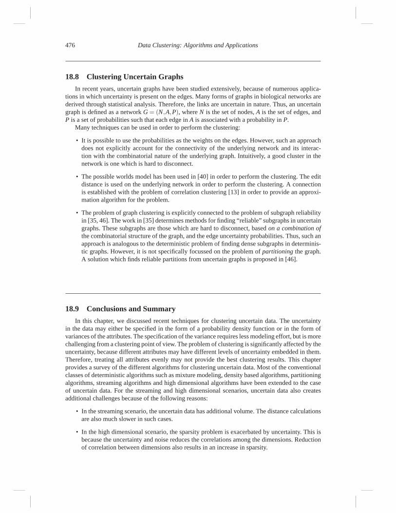
476 Data Clustering: Algorithms and Applications
18.8 Clustering Uncertain Graphs
In recent years, uncertain graphs have been studied extensively, because of numerous applica-tions in which uncertainty is present on the edges. Many forms of graphs in biological networks arederived through statistical analysis. Therefore, the links are uncertain in nature. Thus, an uncertaingraph is defined as a network G = (N,A,P), where N is the set of nodes, A is the set of edges, andP is a set of probabilities such that each edge in A is associated with a probability in P.
Many techniques can be used in order to perform the clustering:
• It is possible to use the probabilities as the weights on the edges. However, such an approachdoes not explicitly account for the connectivity of the underlying network and its interac-tion with the combinatorial nature of the underlying graph. Intuitively, a good cluster in thenetwork is one which is hard to disconnect.
• The possible worlds model has been used in [40] in order to perform the clustering. The editdistance is used on the underlying network in order to perform the clustering. A connectionis established with the problem of correlation clustering [13] in order to provide an approxi-mation algorithm for the problem.
• The problem of graph clustering is explicitly connected to the problem of subgraph reliabilityin [35, 46]. The work in [35] determines methods for finding “reliable” subgraphs in uncertaingraphs. These subgraphs are those which are hard to disconnect, based on a combination ofthe combinatorial structure of the graph, and the edge uncertainty probabilities. Thus, such anapproach is analogous to the deterministic problem of finding dense subgraphs in determinis-tic graphs. However, it is not specifically focussed on the problem of partitioning the graph.A solution which finds reliable partitions from uncertain graphs is proposed in [46].
18.9 Conclusions and Summary
In this chapter, we discussed recent techniques for clustering uncertain data. The uncertaintyin the data may either be specified in the form of a probability density function or in the form ofvariances of the attributes. The specification of the variance requires less modeling effort, but is morechallenging from a clustering point of view. The problem of clustering is significantly affected by theuncertainty, because different attributes may have different levels of uncertainty embedded in them.Therefore, treating all attributes evenly may not provide the best clustering results. This chapterprovides a survey of the different algorithms for clustering uncertain data. Most of the conventionalclasses of deterministic algorithms such as mixture modeling, density based algorithms, partitioningalgorithms, streaming algorithms and high dimensional algorithms have been extended to the caseof uncertain data. For the streaming and high dimensional scenarios, uncertain data also createsadditional challenges because of the following reasons:
• In the streaming scenario, the uncertain data has additional volume. The distance calculationsare also much slower in such cases.
• In the high dimensional scenario, the sparsity problem is exacerbated by uncertainty. This isbecause the uncertainty and noise reduces the correlations among the dimensions. Reductionof correlation between dimensions also results in an increase in sparsity.
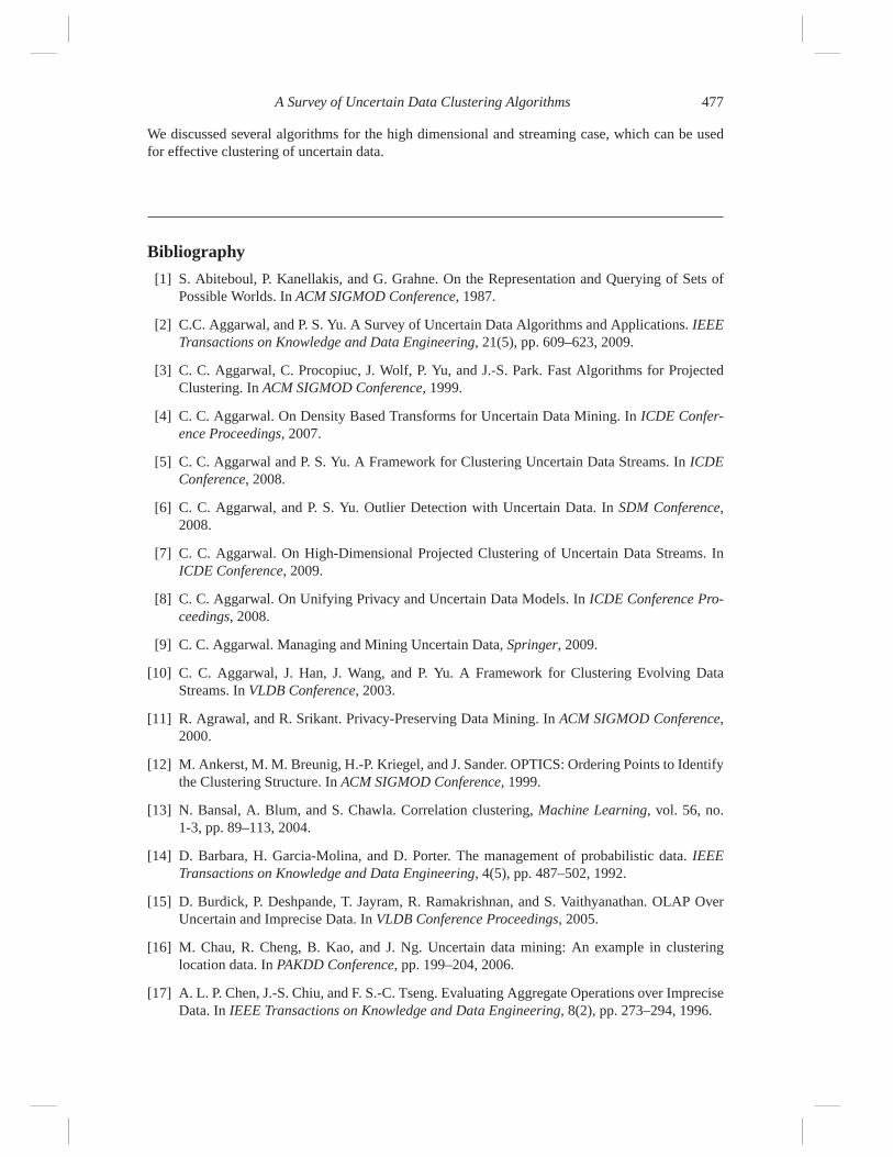
A Survey of Uncertain Data Clustering Algorithms 477
We discussed several algorithms for the high dimensional and streaming case, which can be usedfor effective clustering of uncertain data.
Bibliography
[1] S. Abiteboul, P. Kanellakis, and G. Grahne. On the Representation and Querying of Sets ofPossible Worlds. In ACM SIGMOD Conference, 1987.
[2] C.C. Aggarwal, and P. S. Yu. A Survey of Uncertain Data Algorithms and Applications. IEEETransactions on Knowledge and Data Engineering, 21(5), pp. 609–623, 2009.
[3] C. C. Aggarwal, C. Procopiuc, J. Wolf, P. Yu, and J.-S. Park. Fast Algorithms for ProjectedClustering. In ACM SIGMOD Conference, 1999.
[4] C. C. Aggarwal. On Density Based Transforms for Uncertain Data Mining. In ICDE Confer-ence Proceedings, 2007.
[5] C. C. Aggarwal and P. S. Yu. A Framework for Clustering Uncertain Data Streams. In ICDEConference, 2008.
[6] C. C. Aggarwal, and P. S. Yu. Outlier Detection with Uncertain Data. In SDM Conference,2008.
[7] C. C. Aggarwal. On High-Dimensional Projected Clustering of Uncertain Data Streams. InICDE Conference, 2009.
[8] C. C. Aggarwal. On Unifying Privacy and Uncertain Data Models. In ICDE Conference Pro-ceedings, 2008.
[9] C. C. Aggarwal. Managing and Mining Uncertain Data, Springer, 2009.
[10] C. C. Aggarwal, J. Han, J. Wang, and P. Yu. A Framework for Clustering Evolving DataStreams. In VLDB Conference, 2003.
[11] R. Agrawal, and R. Srikant. Privacy-Preserving Data Mining. In ACM SIGMOD Conference,2000.
[12] M. Ankerst, M. M. Breunig, H.-P. Kriegel, and J. Sander. OPTICS: Ordering Points to Identifythe Clustering Structure. In ACM SIGMOD Conference, 1999.
[13] N. Bansal, A. Blum, and S. Chawla. Correlation clustering, Machine Learning, vol. 56, no.1-3, pp. 89–113, 2004.
[14] D. Barbara, H. Garcia-Molina, and D. Porter. The management of probabilistic data. IEEETransactions on Knowledge and Data Engineering, 4(5), pp. 487–502, 1992.
[15] D. Burdick, P. Deshpande, T. Jayram, R. Ramakrishnan, and S. Vaithyanathan. OLAP OverUncertain and Imprecise Data. In VLDB Conference Proceedings, 2005.
[16] M. Chau, R. Cheng, B. Kao, and J. Ng. Uncertain data mining: An example in clusteringlocation data. In PAKDD Conference, pp. 199–204, 2006.
[17] A. L. P. Chen, J.-S. Chiu, and F. S.-C. Tseng. Evaluating Aggregate Operations over ImpreciseData. In IEEE Transactions on Knowledge and Data Engineering, 8(2), pp. 273–294, 1996.
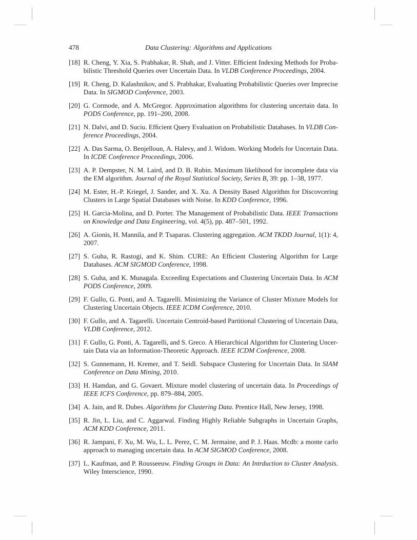
478 Data Clustering: Algorithms and Applications
[18] R. Cheng, Y. Xia, S. Prabhakar, R. Shah, and J. Vitter. Efficient Indexing Methods for Proba-bilistic Threshold Queries over Uncertain Data. In VLDB Conference Proceedings, 2004.
[19] R. Cheng, D. Kalashnikov, and S. Prabhakar, Evaluating Probabilistic Queries over ImpreciseData. In SIGMOD Conference, 2003.
[20] G. Cormode, and A. McGregor. Approximation algorithms for clustering uncertain data. InPODS Conference, pp. 191–200, 2008.
[21] N. Dalvi, and D. Suciu. Efficient Query Evaluation on Probabilistic Databases. In VLDB Con-ference Proceedings, 2004.
[22] A. Das Sarma, O. Benjelloun, A. Halevy, and J. Widom. Working Models for Uncertain Data.In ICDE Conference Proceedings, 2006.
[23] A. P. Dempster, N. M. Laird, and D. B. Rubin. Maximum likelihood for incomplete data viathe EM algorithm. Journal of the Royal Statistical Society, Series B, 39: pp. 1–38, 1977.
[24] M. Ester, H.-P. Kriegel, J. Sander, and X. Xu. A Density Based Algorithm for DiscovceringClusters in Large Spatial Databases with Noise. In KDD Conference, 1996.
[25] H. Garcia-Molina, and D. Porter. The Management of Probabilistic Data. IEEE Transactionson Knowledge and Data Engineering, vol. 4(5), pp. 487–501, 1992.
[26] A. Gionis, H. Mannila, and P. Tsaparas. Clustering aggregation. ACM TKDD Journal, 1(1): 4,2007.
[27] S. Guha, R. Rastogi, and K. Shim. CURE: An Efficient Clustering Algorithm for LargeDatabases. ACM SIGMOD Conference, 1998.
[28] S. Guha, and K. Munagala. Exceeding Expectations and Clustering Uncertain Data. In ACMPODS Conference, 2009.
[29] F. Gullo, G. Ponti, and A. Tagarelli. Minimizing the Variance of Cluster Mixture Models forClustering Uncertain Objects. IEEE ICDM Conference, 2010.
[30] F. Gullo, and A. Tagarelli. Uncertain Centroid-based Partitional Clustering of Uncertain Data,VLDB Conference, 2012.
[31] F. Gullo, G. Ponti, A. Tagarelli, and S. Greco. A Hierarchical Algorithm for Clustering Uncer-tain Data via an Information-Theoretic Approach. IEEE ICDM Conference, 2008.
[32] S. Gunnemann, H. Kremer, and T. Seidl. Subspace Clustering for Uncertain Data. In SIAMConference on Data Mining, 2010.
[33] H. Hamdan, and G. Govaert. Mixture model clustering of uncertain data. In Proceedings ofIEEE ICFS Conference, pp. 879–884, 2005.
[34] A. Jain, and R. Dubes. Algorithms for Clustering Data. Prentice Hall, New Jersey, 1998.
[35] R. Jin, L. Liu, and C. Aggarwal. Finding Highly Reliable Subgraphs in Uncertain Graphs,ACM KDD Conference, 2011.
[36] R. Jampani, F. Xu, M. Wu, L. L. Perez, C. M. Jermaine, and P. J. Haas. Mcdb: a monte carloapproach to managing uncertain data. In ACM SIGMOD Conference, 2008.
[37] L. Kaufman, and P. Rousseeuw. Finding Groups in Data: An Intrduction to Cluster Analysis.Wiley Interscience, 1990.
A Survey of Uncertain Data Clustering Algorithms 479
[38] R. Ng and J. Han. Efficient and Effective Clustering Algorithms for Spatial Data Mining. InVLDB Conference, 1994.
[39] B. Kao, S. D. Lee, D. W. Cheung, W. S. Ho, K. F. Chan. Clustering Uncertain Data usingVoronoi Diagrams. In IEEE ICDM Conference, 2008.
[40] G. Kollios, M. Potamias, and E. Terzi. Clustering Large Probabilistic Graphs, IEEE TKDEJournal, to appear.
[41] M. Kumar, N. Patel, and J. Woo. Clustering seasonality patterns in the presence of errors. InACM KDD Conference Proceedings, pp. 557–563, 2002.
[42] H.-P. Kriegel, and M. Pfeifle. Density-Based Clustering of Uncertain Data. In ACM KDDConference Proceedings, 2005.
[43] H.-P. Kriegel, and M. Pfeifle. Hierarchical Density Based Clustering of Uncertain Data. InICDM Conference, 2005.
[44] L. V. S. Lakshmanan, N. Leone, R. Ross, and V. S. Subrahmanian. ProbView: A FlexibleProbabilistic Database System. ACM Transactions on Database Systems, 22(3), pp. 419–469,1997.
[45] S. D. Lee, B. Kao, and R. Cheng. Reducing UK-means to K-means. In ICDM Workshops,2006.
[46] L. Liu, R. Jin, C. Aggarwal, and Y. Shen. Reliable Clustering on Uncertain Graphs, ICDMConference, 2012.
[47] S. I. McClean, B. W. Scotney, and M. Shapcott. Aggregation of Imprecise and Uncertain In-formation in Databases. IEEE Transactions on Knowledge and Data Engineering, 13(6), pp.902–912, 2001.
[48] W. Ngai, B. Kao, C. Chui, R. Cheng, M. Chau, and K. Y. Yip. Efficient Clustering of UncertainData. In ICDM Conference Proceedings, 2006.
[49] D. Pfozer, and C. Jensen. Capturing the uncertainty of moving object representations. In SSDMConference, 1999.
[50] M. Sato, Y. Sato, and L. Jain. Fuzzy Clustering Models and Applications. Physica–Verlag,Heidelberg, 1997.
[51] S. Singh, C. Mayfield, S. Prabhakar, R. Shah, and S. Hambrusch. Indexing Uncertain Categor-ical Data. In ICDE Conference, 2007.
[52] Y. Tao, R. Cheng, X. Xiao, W. Ngai, B. Kao, and S. Prabhakar. Indexing Multi-dimensionalUncertain Data with Arbitrary Probabality Density Functions. In VLDB Conference, 2005.
[53] P. Volk, F. Rosenthal, M. Hahmann, D. Habich, and W. Lehner. Clustering Uncertain Data withPossible Worlds. ICDE Conference, 2009.
[54] L. Xiao, and E. Hung. An Efficient Distance Calculation Method between Uncertain Objects,CIDM Conference, 2007.
[55] C. Zhang, M. Gao, and A. Zhou. Tracking High Quality Clusters over Uncertain Data Streams,ICDE Conference, 2009.
[56] T. Zhang, R. Ramakrishnan, and M. Livny. BIRCH: An Efficient Data Clustering Method forVery Large Databases. In ACM SIGMOD Conference Proceedings, 1996.


![Cluster Analysis - uni-bielefeld.deRepresentative-based clustering [Aggarwal 2015, section 6.3] Probabilistic model-based clustering [Section 6.5] Hierarchical clustering [Section](https://static.fdocuments.in/doc/165x107/5f7050d1e8c3ea15a658d1e4/cluster-analysis-uni-representative-based-clustering-aggarwal-2015-section.jpg)


![Efficient and Effective Algorithms for Clustering Uncertain Graphs · 2019-07-12 · tic network (or delay tolerant network) [15, 28, 48] can be mod-eled as uncertain graphs where](https://static.fdocuments.in/doc/165x107/5e38661237823439b041e274/eficient-and-effective-algorithms-for-clustering-uncertain-2019-07-12-tic-network.jpg)


![Entrepreneurial Exits and Innovation - INSEADfaculty.insead.edu/vikas-aggarwal/documents/[3] Aggarwal, Hsu (2014... · Entrepreneurial Exits and Innovation Vikas A. Aggarwal ... and](https://static.fdocuments.in/doc/165x107/5a9f222e7f8b9a71178c5b59/entrepreneurial-exits-and-innovation-3-aggarwal-hsu-2014entrepreneurial.jpg)