UNIVERSITY OF OULU P .O. Box 8000 F I -90014 UNIVERSITY OF OULU FINLAND

A C T A U N I V E R S I T A T I S O U L U E N S I S

University Lecturer Tuomo Glumoff

University Lecturer Santeri Palviainen

Postdoctoral researcher Jani Peräntie

University Lecturer Anne Tuomisto

University Lecturer Veli-Matti Ulvinen

Planning Director Pertti Tikkanen

Professor Jari Juga

University Lecturer Anu Soikkeli

University Lecturer Santeri Palviainen

Publications Editor Kirsti Nurkkala

ISBN 978-952-62-2784-9 (Paperback)ISBN 978-952-62-2785-6 (PDF)ISSN 0355-3213 (Print)ISSN 1796-2226 (Online)

U N I V E R S I TAT I S O U L U E N S I SACTAC

TECHNICA

U N I V E R S I TAT I S O U L U E N S I SACTAC

TECHNICA

OULU 2020

C 771

Janne Mustaniemi

COMPUTER VISION METHODS FOR MOBILE IMAGING AND 3D RECONSTRUCTION

UNIVERSITY OF OULU GRADUATE SCHOOL;UNIVERSITY OF OULU,FACULTY OF INFORMATION TECHNOLOGY AND ELECTRICAL ENGINEERING

C 771

AC

TAJanne M

ustaniemi

C771etukansi.fm Page 1 Monday, November 2, 2020 11:30 AM

ACTA UNIVERS ITAT I S OULUENS I SC Te c h n i c a 7 7 1

JANNE MUSTANIEMI

COMPUTER VISION METHODSFOR MOBILE IMAGING AND 3D RECONSTRUCTION

Academic dissertation to be presented with the assent ofthe Doctoral Training Committee of InformationTechnology and Electrical Engineering of the Universityof Oulu for public defence in the OP auditorium (L10),Linnanmaa, on 4 December 2020, at 12 noon

UNIVERSITY OF OULU, OULU 2020

Copyright © 2020Acta Univ. Oul. C 771, 2020

Supervised byProfessor Janne HeikkiläAssistant Professor Juho Kannala

Reviewed byAssociate Professor Filip SroubekAssociate Professor Atsuto Maki

ISBN 978-952-62-2784-9 (Paperback)ISBN 978-952-62-2785-6 (PDF)

ISSN 0355-3213 (Printed)ISSN 1796-2226 (Online)

Cover DesignRaimo Ahonen

PUNAMUSTATAMPERE 2020

OpponentProfessor Joni-Kristian Kämäräinen

Mustaniemi, Janne, Computer vision methods for mobile imaging and 3Dreconstruction. University of Oulu Graduate School; University of Oulu, Faculty of Information Technologyand Electrical EngineeringActa Univ. Oul. C 771, 2020University of Oulu, P.O. Box 8000, FI-90014 University of Oulu, Finland

Abstract

This thesis presents novel computer vision methods for improving image-based 3D reconstructionand mobile photography. Devices such as smartphones and tablets are commonly equipped withan inertial measurement unit (IMU) that provides information about the motion of the device.Moreover, many devices can be programmed to capture rapid bursts of images with differentexposure times. The methods introduced utilize multi-modal and complementary informationacquirable with mobile devices.

Three-dimensional scene reconstruction from multiple images is an essential problem incomputer vision. This process has a well-known limitation that the absolute scale of thereconstruction cannot be recovered using a single camera. This thesis presents an inertial-basedscale estimation method that recovers the unknown scale factor. The method achieves state-of-the-art performance and can easily be integrated with existing 3D reconstruction software.

Motion blur is a common issue when capturing images in low light conditions. It not onlydegrades the visual quality but damages various computer vision applications, including image-based 3D reconstruction. This thesis presents two deblurring methods for removing spatiallyvariant motion blur using inertial measurements. Unlike most of the existing approaches, themethods are capable of running in real-time. This thesis also investigates the problem of jointdenoising and deblurring. It introduces a novel learning-based approach to recovering sharp andnoise-free photographs from a pair of short and long exposure images.

Multi-aperture cameras have become common in smartphones. The use of multiple cameraunits provides another way to improve image quality and camera features. This thesis explores theproblem of parallax correction caused by each camera unit having a slightly different viewpoint.This work presents an image fusion algorithm for a particular multi-aperture camera where cameraunits have different color filters. The images are fused using a disparity map that is estimated whileconsidering all images simultaneously. The approach is a feasible alternative to traditionalcameras equipped with a Bayer filter.

Keywords: computational photography, image deblurring, image denoising, inertialmeasurement unit, multi-aperture camera, scale estimation

Mustaniemi, Janne, Konenäön menetelmiä mobiilikuvantamiseen ja 3D-rekonst-ruktioon. Oulun yliopiston tutkijakoulu; Oulun yliopisto, Tieto- ja sähkötekniikan tiedekuntaActa Univ. Oul. C 771, 2020Oulun yliopisto, PL 8000, 90014 Oulun yliopisto

Tiivistelmä

Tässä väitöskirjassa esitellään uusia konenäön menetelmiä, jotka pyrkivät parantamaan kuva-pohjaista 3D-rekonstruktiota ja mobiilivalokuvausta. Laitteet, kuten älypuhelimet ja tablet-tieto-koneet sisältävät yleensä inertiamittausyksikön, joka antaa tietoa laitteen liikkeestä. Lisäksimonilla laitteilla on mahdollista ottaa useita kuvia nopeasti peräkkäin eri valotusajoilla. Työssäesitetyt menetelmät hyödyntävät mobiililaitteiden eri sensoreilla saatavaa multimodaalista ja toi-siaan täydentävää tietoa.

Kuvapohjainen 3D-rekonstruktio on eräs konenäön keskeisimmistä ongelmista. Tähän pro-sessiin liittyy tunnettu rajoitus, että 3D-mallin absoluuttista skaalaa ei voida määrittää pelkästäänyhden kameran avulla. Tämä työ esittelee inertiaalipohjaisen menetelmän, jolla tuntematonskaalauskerroin voidaan määrittää. Menetelmällä saadut tulokset ovat ensiluokkaisia ja menetel-mä voidaan helposti integroida olemassa oleviin 3D-rekonstruktio-ohjelmistoihin.

Liike-epäterävyys on ongelma, joka ilmenee usein hämärässä kuvattaessa. Se huonontaavalokuvien laatua ja vaikuttaa negatiivisesti moniin konenäön sovelluksiin, kuten kuvapohjai-seen 3D-rekonstruktioon. Tässä työssä esitellään kaksi menetelmää liike-epäterävyyden pois-toon, jotka hyödyntävät inertiaalimittauksia. Algoritmit ovat reaaliaikaisia, toisin kuin suurin osanykyisistä menetelmistä. Väitöskirjassa tutkitaan myös yhtäaikaista kohinan- ja liike-epäterä-vyydenpoistoa. Se esittää uudenlaisen menetelmän, joka hyödyntää koneoppimista sekä kuvapa-reja, jotka on otettu lyhyellä ja pitkällä valotusajalla.

Moniaukkokamerat ovat yleistyneet älypuhelimissa. Useita kamerayksiköitä hyödyntämällävoidaan parantaa kuvien laatua ja kameran ominaisuuksia. Tässä työssä perehdytään parallaksi-virheen korjaamiseen, mikä aiheutuu siitä, että kamerayksiköiden näkymät eroavat hieman toi-sistaan. Työ esittelee kuvafuusioalgoritmin moniaukkokameraan, missä jokainen kamerayksik-kö on varustettu erillisellä värisuodattimella. Syötekuvat yhdistetään dispariteetti-kartan perus-teella, joka estimoidaan hyödyntämällä kaikkia kuvia yhtä aikaa. Kyseinen lähestymistapa onvarteenotettava vaihtoehto perinteiselle Bayer-suodattimella varustetulle kameralle.

Asiasanat: inertiamittausyksikkö, kohinanpoisto, laskennallinen valokuvaus, liike-epäterävyydenpoisto, moniaukkokamera, skaalan estimointi

To my family and friends

8

Acknowledgements

The research presented in this thesis was carried out in the Center for Machine Visionand Signal Analysis (CMVS) at the University of Oulu between the years 2015 and2020. I wish to express my gratitude to my supervisors Professor Janne Heikkilä andProfessor Juho Kannala. Their guidance, feedback and encouragement has been vitalfor completing this thesis. I am grateful for the freedom they gave me to explore myresearch ideas throughout the studies. At the same time, they knew when to re-direct meback on the appropriate path.

I would like to thank my other co-authors Professor Jiri Matas and Professor SimoSärkkä for all the interesting discussions and ideas. Their constructive feedback helpedme a lot to improve the publications included in this thesis. I am grateful to ProfessorHirokazu Kato and Professor Takafumi Taketomi for their hospitality during my researchvisit at the Nara Institute of Science and Technology (NAIST) in Japan. I wish to thankProfessor Jiri Matas for hosting my visit to the Center for Machine Perception (CMP) atthe Czech Technical University in Prague. Further, I want to acknowledge all othercolleagues at CMVS, NAIST and CMP with whom I have worked.

I acknowledge the follow-up group members Professor Esa Rahtu and Doctor SamiHuttunen for their feedback on studies and research. I am grateful to Doctor DanielHerrera Castro for his guidance at the beginning of my doctoral studies. I would liketo thank pre-examiners Professor Filip Sroubek and Professor Atsuto Maki for theirvaluable feedback. Thank you for investing your time and for sharing your insights. Iam also grateful to Professor Joni-Kristian Kämäräinen for kindly accepting to act as anopponent at my doctoral defense.

I want to acknowledge the FiDiPro programme of Business Finland for the financialsupport that made this research possible. I am also grateful to the Japan Student ServicesOrganization for supporting the research visit to NAIST.

Finally, I want to express my deepest gratitude to my family and friends for all thesupport during these years.

Oulu, September 2020Janne Mustaniemi

9

10

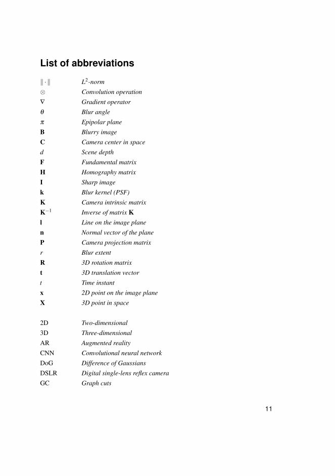
List of abbreviations

‖ · ‖ L2-norm

⊗ Convolution operation

∇ Gradient operator

θ Blur angle

π Epipolar plane

B Blurry image

C Camera center in space

d Scene depth

F Fundamental matrix

H Homography matrix

I Sharp image

k Blur kernel (PSF)

K Camera intrinsic matrix

K−1 Inverse of matrix Kl Line on the image plane

n Normal vector of the plane

P Camera projection matrix

r Blur extent

R 3D rotation matrix

t 3D translation vector

t Time instant

x 2D point on the image plane

X 3D point in space

2D Two-dimensional

3D Three-dimensional

AR Augmented reality

CNN Convolutional neural network

DoG Difference of Gaussians

DSLR Digital single-lens reflex camera

GC Graph cuts

11

GPU Graphics processing unit

HDR High dynamic range

HMI Hierarchical mutual information

IMU Inertial measurement unit

IRLS Iteratively reweighted least squares

LSD2 Long-short denoising and deblurring

MI Mutual information

NCC Normalized cross-correlation

NIR Near-infrared

OIS Optical image stabilization

PSF Point spread function

RANSAC Random sample consensus

RGB Red, green and blue

RTS Rauch-Tung-Striebel

SAD Sum of absolute differences

SGM Semi-global matching

SfM Structure-from-motion

SIFT Scale invariant feature transform

SLAM Simultaneous localization and mapping

ToF Time-of-flight

VR Virtual reality

12

List of original publications

This dissertation is based on the following articles which are referred to in the text bytheir Roman numerals (I–V):

I Mustaniemi J, Kannala J, Särkkä S, Matas J & Heikkilä J (2017, September) Inertial-based scale estimation for structure from motion on mobile devices. IEEE/RSJ Interna-tional Conference on Intelligent Robots and Systems (IROS). Vancouver, BC, Canada.https://doi.org/10.1109/IROS.2017.8206303

II Mustaniemi J, Kannala J, Särkkä S, Matas J & Heikkilä J (2018, August) Fast motion de-blurring for feature detection and matching using inertial measurements. 24th InternationalConference on Pattern Recognition (ICPR). Beijing, China.https://doi.org/10.1109/ICPR.2018.8546041

III Mustaniemi J, Kannala J, Särkkä S, Matas J & Heikkilä J (2019, January) Gyroscope-aidedmotion deblurring with deep networks. IEEE Winter Conference on Applications ofComputer Vision (WACV). Waikoloa Village, Hawaii, USA.https://doi.org/10.1109/WACV.2019.00208

IV Mustaniemi J, Kannala J, Matas J, Särkkä S & Heikkilä J (2020, September) LSD2 - Jointdenoising and deblurring of short and long exposure images with CNNs. The BritishMachine Vision Virtual Conference (BMVC). https://arxiv.org/abs/1811.09485

V Mustaniemi J, Kannala J & Heikkilä J (2016) Parallax correction via disparity estima-tion in a multi-aperture camera. Machine Vision and Applications, 27(8), 1313–1323.https://doi.org/10.1007/s00138-016-0773-7

The author of this dissertation had the main responsibility of preparing articles I-V.This includes the implementation of the algorithms, experiments, and writing. The ideaspresented in the articles were devised in group discussions with the co-authors, duringwhich they provided valuable suggestions and feedback.

13

14

Contents

AbstractTiivistelmäAcknowledgements 9List of abbreviations 11List of original publications 13Contents 151 Introduction 17

1.1 Background and motivation . . . . . . . . . . . . . . . . . . . . . . . . . . . . . . . . . . . . . . . . . . . 17

1.2 Scope of the thesis . . . . . . . . . . . . . . . . . . . . . . . . . . . . . . . . . . . . . . . . . . . . . . . . . . . 18

1.3 Contributions . . . . . . . . . . . . . . . . . . . . . . . . . . . . . . . . . . . . . . . . . . . . . . . . . . . . . . . . 19

1.4 Overview of original articles . . . . . . . . . . . . . . . . . . . . . . . . . . . . . . . . . . . . . . . . . . 20

1.5 Outline of the thesis . . . . . . . . . . . . . . . . . . . . . . . . . . . . . . . . . . . . . . . . . . . . . . . . . . 21

2 Image-based 3D reconstruction with handheld devices 232.1 Multiple-view geometry . . . . . . . . . . . . . . . . . . . . . . . . . . . . . . . . . . . . . . . . . . . . . . 24

2.1.1 Two-view geometry . . . . . . . . . . . . . . . . . . . . . . . . . . . . . . . . . . . . . . . . . . . 24

2.1.2 Three-view geometry . . . . . . . . . . . . . . . . . . . . . . . . . . . . . . . . . . . . . . . . . . 24

2.2 Structure from motion . . . . . . . . . . . . . . . . . . . . . . . . . . . . . . . . . . . . . . . . . . . . . . . . 26

2.2.1 Scale ambiguity . . . . . . . . . . . . . . . . . . . . . . . . . . . . . . . . . . . . . . . . . . . . . . . 27

2.3 Scale estimation . . . . . . . . . . . . . . . . . . . . . . . . . . . . . . . . . . . . . . . . . . . . . . . . . . . . . 28

2.3.1 Inertial-based scale estimation . . . . . . . . . . . . . . . . . . . . . . . . . . . . . . . . . . 29

2.3.2 Scale estimation on mobile devices . . . . . . . . . . . . . . . . . . . . . . . . . . . . . . 31

2.3.3 Discussion . . . . . . . . . . . . . . . . . . . . . . . . . . . . . . . . . . . . . . . . . . . . . . . . . . . . 32

3 Low-light imaging with handheld devices 353.1 Motion blur . . . . . . . . . . . . . . . . . . . . . . . . . . . . . . . . . . . . . . . . . . . . . . . . . . . . . . . . . 36

3.2 Image deblurring . . . . . . . . . . . . . . . . . . . . . . . . . . . . . . . . . . . . . . . . . . . . . . . . . . . . .37

3.2.1 Non-blind deblurring . . . . . . . . . . . . . . . . . . . . . . . . . . . . . . . . . . . . . . . . . . 38

3.2.2 Blind deblurring . . . . . . . . . . . . . . . . . . . . . . . . . . . . . . . . . . . . . . . . . . . . . . . 39

3.3 Inertial-aided deblurring . . . . . . . . . . . . . . . . . . . . . . . . . . . . . . . . . . . . . . . . . . . . . . 40

3.3.1 Fast motion deblurring . . . . . . . . . . . . . . . . . . . . . . . . . . . . . . . . . . . . . . . . . 41

3.3.2 Deblurring with deep networks . . . . . . . . . . . . . . . . . . . . . . . . . . . . . . . . . 42

3.3.3 Discussion . . . . . . . . . . . . . . . . . . . . . . . . . . . . . . . . . . . . . . . . . . . . . . . . . . . . 44

15

3.4 Multi-image restoration. . . . . . . . . . . . . . . . . . . . . . . . . . . . . . . . . . . . . . . . . . . . . . .443.4.1 Joint denoising and deblurring . . . . . . . . . . . . . . . . . . . . . . . . . . . . . . . . . . 463.4.2 Discussion . . . . . . . . . . . . . . . . . . . . . . . . . . . . . . . . . . . . . . . . . . . . . . . . . . . . 48

4 Multi-aperture imaging 514.1 Advantages of multi-aperture imaging . . . . . . . . . . . . . . . . . . . . . . . . . . . . . . . . . . 514.2 Existing multi-aperture cameras . . . . . . . . . . . . . . . . . . . . . . . . . . . . . . . . . . . . . . . 534.3 Stereo matching . . . . . . . . . . . . . . . . . . . . . . . . . . . . . . . . . . . . . . . . . . . . . . . . . . . . . 54

4.3.1 Matching costs . . . . . . . . . . . . . . . . . . . . . . . . . . . . . . . . . . . . . . . . . . . . . . . . 554.3.2 Disparity estimation . . . . . . . . . . . . . . . . . . . . . . . . . . . . . . . . . . . . . . . . . . . 56

4.4 Parallax correction in a multi-aperture camera . . . . . . . . . . . . . . . . . . . . . . . . . . 594.5 Discussion . . . . . . . . . . . . . . . . . . . . . . . . . . . . . . . . . . . . . . . . . . . . . . . . . . . . . . . . . . 60

5 Summary and conclusion 63References 65Original publications 75

16

1 Introduction

1.1 Background and motivation

Computer vision aims to give computers the ability to see, identify, and process thecontent of digital images. It is a broad and diverse subject that is being used in manyreal-world applications including medical imaging, industrial inspection, surveillance,3D modeling, and automotive safety (Szeliski, 2010). Mobile devices have becomeattractive platforms for computer vision applications and smartphones and tablets aregenerally equipped with a camera. Moreover, they often contain various sensors, suchas an inertial measurement unit (IMU), which provide information about the device’smotion. The computational power of mobile devices has also increased considerablyover the years.

The IMU typically includes an accelerometer and a gyroscope. In mobile devices,the IMU is commonly used to enhance human-computer interaction, for example, thescreen of the device can be automatically rotated based on the gravity measured by theaccelerometer. Gyroscope measurements have been used for video stabilization androlling shutter correction (Bell, Troccoli, & Pulli, 2014). Mobile games and applicationsfrequently use the IMU to sense user inputs. Inertial odometry has been demonstratedon smartphones for indoor navigation (Solin, Cortes, Rahtu, & Kannala, 2018). Visual-inertial odometry systems, such as ARKit by Apple, utilize the complementary natureof visual and inertial measurements. These systems are used in applications such asaugmented reality (AR), virtual reality (VR), and autonomous driving.

Real-time 3D reconstruction has been performed on mobile devices (Ondrúška, Kohli,& Izadi, 2015). Building a 3D model of a scene from a collection of photographs enablesvarious applications, for example, a 3D body scan obtained with a smartphone canensure a proper fit when shopping for clothes online (Nettelo Inc., 2019). Nevertheless,the reconstruction process has a well-known limitation which is that the absolute scaleof the reconstruction cannot be recovered using a single camera. The 3D model has tobe scaled before metric measurements can be taken. One solution is to utilize the IMUto recover the unknown scale factor.

Mobile photography can also benefit from the IMU. Taking high-quality photographswith a handheld smartphone camera is challenging, especially in low-light conditions.The optics of the camera need to be small, which limits the amount of light reaching the

17

sensor. It is often necessary to use longer exposure time to improve the signal-to-noiseratio. With a handheld camera, this can introduce motion blur that degrades the qualityof the image. Motion information from the IMU has been used for removing motionblur caused by handshake (Zhang & Hirakawa, 2016).

Another disadvantage of smartphone cameras is that they have a low dynamic rangecompared to digital single-lens reflex (DSLR) cameras. They also cannot produceimages with shallow depth of field because of the small aperture (Tallon, 2016). Mobiledevices can often be programmed to capture bursts of images in rapid succession. TheNight Sight camera mode in Google Pixel smartphones combines information frommultiple images to reduce image noise and to increase dynamic range (Liba et al., 2019).Furthermore, some camera applications let the user change the point of focus and depthof field after the photograph has been taken (Lens Blur, 2014).

Most modern high-end smartphones have multiple back-facing cameras. Theseso-called multi-aperture cameras have various advantages compared to traditionalcameras. The camera lenses can have different focal lengths which allows optical zoomand wide-angle shots. A multi-aperture camera produces multiple images that canbe fused to improve low-light performance and dynamic range. A pair of color andmonochrome cameras has been used to recover noise-free images (Jeon, Lee, Im, Ha,& So Kweon, 2016). Similar to 3D reconstruction, the images taken from differentviewpoints allow depth estimation which enables applications such as post-capturerefocusing, background replacement, resizing of objects, and depth-based color effects.

1.2 Scope of the thesis

This thesis covers a variety of different problems related to 3D reconstruction andmobile imaging. The techniques presented in Papers I-III utilize the IMU that iscommonly found in mobile devices. Paper I addresses the scale ambiguity problemthat is inherent to image-based 3D reconstruction. Motion blur is known to affect thereconstruction process and scale estimation negatively. Papers II-III explore the problemof real-time motion deblurring. Another way to improve mobile imaging is to fuse theinformation from multiple images. Paper IV investigates the problem of joint denoisingand deblurring using short and long exposure images. Image fusion is also essential ina multi-aperture camera. The main challenge is that each camera unit has a slightlydifferent viewpoint, which causes a parallax error (misalignment) between the images.Paper V focuses on parallax correction.

18

1.3 Contributions

The main contributions of the thesis are listed below.

– An inertial-based scale estimation method is proposed that achieves state-of-the-artperformance. The method can cope with inaccurate camera pose estimates and noisyIMU readings and includes an IMU-camera calibration procedure that enables easyintegration with existing 3D reconstruction software. The implementation is publiclyavailable.1 (Paper I)

– An image deblurring method utilizing gyroscope measurements is proposed whichcan handle spatially-variant motion blur and rolling shutter distortion in real time.The method improves the performance of existing feature detectors and descriptorsin the presence of motion blur. This will lead to more accurate and complete 3Dreconstructions. (Paper II)

– An image deblurring method is proposed that incorporates gyroscope measurementsinto a convolutional neural network (CNN). The method produces less deblurringartifacts and overcomes the limitations of IMU-based blur estimation using imagedata. Realistic training data is generated using a gyroscope and sharp photographstaken from the Internet. The implementation is publicly available.2 (Paper III)

– A joint denoising and deblurring method is proposed. The CNN-based approachoutperforms the existing single-image and multi-image methods and allows exposurefusion in the presence of motion blur. A framework is introduced to synthesizerealistic short and long exposure image pairs that are used to train the network. (PaperIV)

– An image fusion algorithm for a multi-aperture camera is proposed. The methodcorrects the parallax error between the images captured with different color filters.Matching costs are combined over multiple images using trifocal tensors to improvedisparity estimation. Post-capture refocusing is also demonstrated using depthinformation that is obtained in the process. (Paper V)

1https://github.com/jannemus/InertialScale2https://github.com/jannemus/DeepGyro

19

1.4 Overview of original articles

Paper I addresses the scale ambiguity problem related to image-based 3D reconstruction.The method recovers the absolute scale of the reconstruction given inertial measurementsand camera poses. The temporal and spatial alignment of the camera and IMU is done inthe process. The scale estimation is performed in the frequency domain which improvesthe robustness against inaccurate sensor timestamps and noisy IMU readings. Themethod utilizes a Rauch-Tung-Striebel (RTS) smoother to cope with inaccurate camerapose estimates typically caused by motion blur and rolling shutter distortion.

Paper II proposes a gyroscope-based deblurring method to improve feature detectionand matching in the presence of motion blur. The method is targeted towards applicationsthat involve a moving camera such as simultaneous localization and mapping (SLAM),VR, and AR. Prior to deblurring, gyro-based blur estimates are validated using imagedata. Wiener deconvolution in the spatial domain is then performed to recover the sharpimage. Unlike existing approaches, the method can handle spatially-variant blur androlling shutter distortion in real time.

Paper III presents a learning-based deblurring method that utilizes gyroscopemeasurements. It is targeted towards similar applications as the method in Paper II. Thesharp image is estimated using a CNN that takes a blurry image and gyro-based blurestimates as input. In general, the blur estimates may be inaccurate due to unknowncamera translation and scene depth, for example. The method uses image data to avoiddeblurring artifacts caused by inaccurate blur estimates.

Paper IV addresses the problem of joint denoising and deblurring. Long exposuretime is often needed in low light conditions to achieve rich colors, good brightness, andlow noise. This can introduce motion blur when the camera is moving (shaking). On theother hand, short exposure time will produce sharp but noisy images. The proposedmethod takes advantage of both images simultaneously using a CNN as well as enablingexposure fusion in the presence of motion blur.

Paper V introduces a multi-aperture camera where each camera unit has a differentcolor filter. The camera is a feasible alternative to a traditional Bayer filter camerain terms of image quality, camera size, and camera features. The paper proposes animage fusion algorithm to correct the parallax error between the sub-images using adisparity map which is estimated from the sub-images. Matching costs are combinedover multiple views using trifocal tensors to improve the disparity map.

20

1.5 Outline of the thesis

This thesis consists of an overview as well as an appendix that contains the originalarticles described in the previous section. The rest of the overview is organized as follows.Chapter 2 describes the background for image-based 3D reconstruction and focuses onthe scale ambiguity problem. Chapter 3 discusses the challenges of low light imagingwith handheld devices with a focus on image deblurring and multi-image restoration.Chapter 4 introduces the existing multi-aperture cameras and their advantages. Thisis followed by a discussion about stereo matching and parallax correction. Chapter 5presents the conclusions.

21

22

2 Image-based 3D reconstruction withhandheld devices

Image-based 3D reconstruction aims to infer the geometric structure of a scene from acollection of images. In the context of stereo matching (Chapter 4), the relative positionand orientation of the cameras (i.e. camera poses) are usually known in advance. Amore challenging problem is when both the 3D structure and camera poses need tobe estimated simultaneously. This is known as structure from motion (SfM). Visualsimultaneous localization and mapping (SLAM) methods solve the analogous problemin real-time. For example, in robotics, there is often a need to determine the position andorientation of a robot with respect to its surroundings while simultaneously building amap of the environment.

There exists many open-source SfM software (Schonberger & Frahm, 2016; Wu,2011) and SLAM software (Mur-Artal & Tardós, 2017a; Sumikura, Shibuya, & Sakurada,2019). Large-scale reconstruction systems have been developed that can utilize thousandsor millions of Internet photos (Heinly, Schonberger, Dunn, & Frahm, 2015). The filmindustry uses SfM techniques to superimpose 3D graphics or computer-generated images(CGI) on a scene. With software such as RealityCapture (Capturing Reality, 2020), onecan create authentic digital 3D assets for games and movies. In the games industry,these techniques have been used to create realistic virtual worlds. There are variousother use cases for these applications, including the creation of 3D maps and modelsfrom drone images. Real-time 3D reconstruction has also been demonstrated on mobiledevices (Ondrúška et al., 2015).

Robot navigation, virtual reality (VR), and augmented reality (AR) applications oftenemploy SLAM techniques. Many of the recent VR headsets use inside-out positionaltracking enabled by SLAM. This approach eliminates the need for external cameras,sensors and markers that would otherwise need to be placed in the environment. AR is atechnology that aims to bridge the gap between virtual and real-world environments.The user can see the real-world while virtual 3D objects are seamlessly overlaid ontop of it. This can be useful, for example, in applications related to maintenance andrepair, medical visualization, and entertainment. Smartphones and tablets are suitableplatforms for AR. Some companies have also developed mixed reality headsets, such asMicrosoft’s HoloLens 2.

23

2.1 Multiple-view geometry

The human visual system uses various monocular and binocular cues to perceive depth.Observing a scene with both eyes provides binocular depth cues. Two slightly differentimages are formed on the retinas of the eyes. The brain seamlessly uses binoculardisparity, also known as parallax, for depth perception. Similarly, the aim of image-based3D reconstruction is to extract depth information from images captured from differentviewpoints. An essential step in this process is to identify the corresponding points(pixels) from each image. Once the correspondences have been established, the 3Dposition of each point can be determined via triangulation, assuming that camera posesare known.

2.1.1 Two-view geometry

The epipolar geometry between two views provides a very useful constraint that helpsto identify the corresponding image points. Consider the stereo vision system in Fig.1(a). A 3D point X is projected onto the image planes of the cameras. Given the 2Dprojection x in the first image, the objective is to find the corresponding point x′ in thesecond image. The point X and camera centers C and C′ form an epipolar plane π

that intersects both image planes. The intersection lines l and l′ are called the epipolarlines. The epipolar geometry simplifies the search problem because the point x has itscorresponding point x′ somewhere on the epipolar line l′. This line can be computedusing a 3×3 fundamental matrix F, which encapsulates the intrinsic projective geometrybetween two views. For all corresponding points, it holds that

x′>Fx = 0. (1)

The fundamental matrix can be estimated from at least seven corresponding imagepoints (Hartley & Zisserman, 2003). A sparse set of correspondences can be obtainedusing feature detection and matching as will be discussed in Section 2.2. Alternatively,the fundamental matrix can be constructed from the camera matrices if the cameras havebeen calibrated.

2.1.2 Three-view geometry

A fundamental matrix relates the corresponding points in stereo images. In the case ofthree views, this role is played by the trifocal tensor. It can be expressed by a set of three

24

Fig. 1. Multiple view geometry. (a) The epipolar geometry between two views states thatgiven a point x in the first view, the corresponding point in the second view x′ must lie onthe epipolar line l′. (b) In the case of three views, the point in the third view x′′ is determinedgiven a correspondence x↔ x′. The point x can be transferred to the third view via a planeπ ′ defined by the back-projection of the line l′. Any line l′ through point x′ in the second viewinduces a homography between the first and third views.

3 × 3 matrices. Similar to the fundamental matrix, the trifocal tensor is independent ofthe scene structure and encapsulates all the geometric relations between the three views.The trifocal tensor can be constructed from the camera matrices or, if the cameras havenot been calibrated, it can be estimated from at least six point correspondences. (Hartley& Zisserman, 2003)

The trifocal tensor can be used to transfer points from a correspondence in twoviews to the corresponding point in a third view. A similar transfer property also holdsfor lines. The point transfer is illustrated in Fig. 1(b). Given a pair of correspondingpoints x and x′, the corresponding point in the third view x′′ can be determined. Let l′

be some line in the second image that goes through the known point x′. The plane π ′

is formed by back-projecting the line l′ to 3D space. The center of the first camera Cand point x define a ray in 3D space that intersects π ′ in the point X. This point is thenimaged as the point x′′ in the third view. It should be noted that the line l′ should not bethe epipolar line corresponding to point x. In such cases, the intersection between theplane π ′ and ray through point x is not defined. For the mathematical details, the readeris referred to the book by Hartley and Zisserman (2003).

25

2.2 Structure from motion

Structure from motion (SfM) is the process of estimating the 3D structure of a scenefrom images taken from different viewpoints. To solve the problem, both the 3Dstructure and camera poses need to be estimated. The internal camera parameters, suchas the focal length, may also be unknown and vary between the images. Incremental SfMis arguably the most popular approach for reconstructing unordered photo collections(Schonberger & Frahm, 2016). New images are incorporated into the reconstruction oneat a time. An overview of an incremental SfM pipeline is shown in Fig. 2.

The SfM process typically starts with feature extraction and matching. A sparseset of point-like features can be extracted from the images using a keypoint detectorsuch as the Difference of Gaussians (DoG) (Lowe et al., 1999). After the keypointdetection, feature descriptors are extracted. The neighborhood of each keypoint is turnedinto a descriptor that works as an identifier. The idea is that the same region can beidentified from each image regardless of the changes in viewpoint and lighting. ScaleInvariant Feature Transform (SIFT) (Lowe, 2004) is one of the most popular featuredescriptors that is robust to radiometric and geometric changes. In feature matching, thepoint correspondences are established between the images by finding the most similardescriptors.

Feature matching is based on visual appearance so there is no guarantee that twomatched features correspond to the same 3D point. Corresponding points must satisfythe epipolar constraint as described in Section 2.1.1. Potentially overlapping images areverified by estimating the fundamental matrix between an image pair. For calibratedcameras, the essential matrix can be estimated instead. A robust estimation method, suchas RANSAC (Fischler & Bolles, 1981), can be used to eliminate outliers, i.e. the pointsthat do not satisfy the epipolar constraint. The image pair is considered geometricallyverified if there are a sufficient amount of inliers.

The incremental reconstruction process is initialized from a carefully selected imagepair. Initializing from a pair with many overlapping cameras typically results in a morerobust and accurate reconstruction. Given the image correspondences xi ↔ x′i, theobjective is to find the camera matrices P and P′ as well as the 3D points Xi such that

xi ∼ PXi and x′i ∼ P′Xi for all i. (2)

The general form of a 3 × 4 camera matrix is P = K[R|t], where K is the 3 × 3 intrinsicmatrix containing the internal camera parameters. The rotation matrix R and translation

26

vector t are called the external camera parameters. They define the camera’s orientationand position with respect to the world coordinate frame. The camera matrix describesthe mapping of 3D points in the world to 2D points on the image plane. The symbol"∼" implies that the left and right hand sides are equal up to scale due to the use ofhomogeneous coordinates.

It is generally not possible to recover the absolute position and orientation of thereconstruction. Because of this ambiguity, the first camera is typically chosen to bealigned with the world coordinate frame, that is, P = K[I|0]. The camera matrix P′ canbe extracted from the fundamental matrix (or essential matrix). Another importantobservation is that the absolute distance between the cameras cannot be recoveredfrom the image measurements alone. For calibrated cameras, the reconstruction is thuspossible up to a similarity transformation (rotation, translation and scaling). This is trueregardless of how many points or cameras are used.

Determining the 3D scene points Xi from a set of correspondences is known astriangulation. Geometrically, this means finding the intersection of the optical raysdefined by the camera centers and corresponding image points. Since there may beerrors, for example, in the detected image points, the rays will generally not intersect.Instead, it is possible to find the 3D point that lies nearest to all of the optical rays.

A new image can be registered to the current model by solving the Perspective-n-Point (PnP) problem (Fischler & Bolles, 1981). The objective is to estimate the camerapose (camera matrix) given the triangulated 3D points and 2D points. Again, RANSACis often used since 2D-3D correspondences may be contaminated by outliers. After theimage has been registered, new 3D points may be triangulated.

Image registration and triangulation are separate steps. Errors in the camera posesmay propagate to the triangulated points and vice versa. Bundle adjustment refers to thejoint refinement of camera parameters and structure. The problem is often formulated asa non-linear least squares problem with the goal of minimizing the reprojection error.That is, the distance between the detected 2D points and the projected 3D points shouldbe minimized.

2.2.1 Scale ambiguity

The scale ambiguity is a known limitation of image-based 3D reconstruction. Thereconstruction is only possible up to an unknown scale factor when using a monocularcamera. For example, it is impossible to determine the true height of the bunny in Fig.

27

Fig. 2. General overview of a structure from motion pipeline.

2 based on the images alone. The reconstruction is a scaled version of reality. Thisoriginates from a property of perspective projection that the apparent size of an objectdepends on its distance from the camera. An object twice as large as another one willappear equal in size if it is twice as far away.

Obtaining a scaled 3D reconstruction would be useful in many applications. In 3Dprinting, the user could first scan the object with a mobile device and then print theobject in exact dimensions. A scaled 3D model of a person could ensure a good fitwhen shopping for clothes online. In odometry applications, it might be useful to obtainthe distance traveled in meters. An object recognition system could utilize the scaleinformation to distinguish between two similar objects that differ only in scale.

2.3 Scale estimation

The scale ambiguity problem can be addressed by using additional information aboutthe scene or the camera setup. Sometimes it is possible to place an object with knowndimensions into a scene. Afterwards, the object can be detected and its scale can bepropagated. A mobile application named ImageMeter (Farin, Dirk, 2019) allows the userto make metric measurements from a photograph based on a reference object. SmartMeasure (Smart Tools co., 2019) solves the problem by assuming that the approximateheight of the camera from the ground is known. A similar idea has been used inautonomous driving (Song & Chandraker, 2014). If the camera is mounted on a wheeledvehicle, it is also possible to estimate the scale using the so-called nonholonomicconstraints (Scaramuzza, Fraundorfer, Pollefeys, & Siegwart, 2009). The assumption isthat the camera has a known offset to the vehicle’s center of motion.

An alternative way to recover the scale is by using extra hardware, such as two ormore cameras. The scale is observable if the distance between the cameras (i.e. thebaseline) is known. For instance, Stereo LSD-SLAM proposed by Engel, Stückler,

28

and Cremers (2015) uses a stereo camera to resolve scale ambiguities and difficultieswith degenerate camera motion. It is worth noting that stereo cameras have limitedoperational range. This is especially true with smartphones where cameras are placedclose together.

Global navigation satellite systems (GNSSs) provide metric position measurementsthat can be used to scale the visual reconstruction. Although GNSSs, such as the globalpositioning system (GPS), are typically included in mobile devices, they are relativelyinaccurate. Furthermore, these systems do not work indoors.

An active depth sensor, such as a time-of-flight (ToF) camera, can also be usedto recover the absolute scale. Various SLAM systems utilize an RGB-D camera thatprovides metric per-pixel depth measurements (Schops, Sattler, & Pollefeys, 2019).Active depth sensors are best suited for small-scale and indoor environments due to theirlimited operational range. At present, ToF cameras are still rarely included in mobiledevices.

Ham, Lucey, and Singh (2015) experimented using a speaker and a microphone of amobile device to improve inertial-based scale estimation. The assumption is that there isa large planar surface in the scene from which the sound emitted by the speaker canbounce to the microphone. The metric scale can be inferred by measuring the timedifference between the emitted and received sound given the speed of sound. Thistechnique is known as echolocation.

2.3.1 Inertial-based scale estimation

The fusion of visual and inertial measurements has been a popular research topic in therobotics community. There exist various visual-inertial odometry and SLAM systemsthat can recover the absolute scale based on accelerometer readings. As an example,Mur-Artal and Tardós (2017b) report that the scale error of the trajectory provided bytheir visual-inertial SLAM system is typically below 1%. It may be noted that many ofthese approaches utilize special hardware setups. Test platforms may include a globalshutter camera with wide field-of-view and a high-quality IMU. Proprietary systems,such as ARCore by Google and ARKit by Apple, run on conventional smartphonehardware. Tanskanen et al. (2013) focused on metric 3D reconstruction on hand-helddevices. The authors report that the scale error is up to 10−15%, mostly due to the useof a consumer-grade accelerometer, which was not calibrated.

29

The previously mentioned online approaches require tightly integrated sensor fusion,which leads to relatively complex designs. One has to solve two difficult problems, visualodometry and inertial navigation, simultaneously. Loosely coupled offline methods,such as (Ham, Lucey, & Singh, 2014; Ham et al., 2015; Jung & Taylor, 2001) areadvantageous, as they can be used with any visual reconstruction software. Furthermore,an offline method can use all the data at the same time (i.e. in batch), which can lead toa more accurate scale estimate.

Jung and Taylor (2001) propose an offline method for odometry estimation. First, asmall set of camera poses is obtained from a video sequence. The camera trajectory ismodeled as a spline that has to pass through the camera locations. The spline parametersare chosen so that the predicted accelerations agree with the accelerometer readings.Ham et al. (2014) use existing SfM software to recover the camera poses up to scale,and thereafter fix the scale based on accelerometer readings. This is done by finding ascale factor that minimizes the difference between accelerometer readings and visualaccelerations. In the process, they take advantage of the acceleration caused by gravityto align the camera and IMU temporarily.

30

2.3.2 Scale estimation on mobile devices

Paper I proposes an IMU-based scale estimation method that recovers the absolute scaleof a 3D reconstruction. The 3D structure and camera poses are computed from a videosequence using SfM software. Accelerometer and gyroscope measurements are recordedsimultaneously with the video capture. The processing steps of the algorithm are shownin Fig. 3.

Before the scale estimation, the camera and IMU measurements are aligned inboth temporally and spatially. This is done by comparing angular velocities measuredby the gyroscope and visual angular velocities computed from the camera rotations.The unknown time offset that minimizes the least-squares error between the angularvelocities is chosen as the best estimate. The spatial alignment is performed concurrentlywith the temporal alignment. The IMU coordinate frame is aligned with the cameracoordinate frame by finding the optimal rotation between the angular velocities.

The scale estimation is based on the idea of comparing visual and inertial accelera-tions. The visual accelerations are computed by differentiating the camera positions.The method uses a Rauch-Tung-Striebel (RTS) smoother (Rauch, Tung, & Striebel,1965) to cope with noisy position estimates. The RTS smoother is a two-pass algorithmthat utilizes future samples to determine the optimal smoothing. The forward passcorresponds to the Kalman filter (Kalman, 1960), which takes into account that thedevice is expected to follow physical laws of motion. The estimates of the state and thecovariances are stored for the backward pass.

Visual and inertial accelerations are compared in the camera coordinate frame. Thecomparison is complicated by the fact that an accelerometer not only measures theacceleration caused by motion but also the earth’s gravity, which is not observed by thecamera. Moreover, the IMU readings are corrupted by noise and bias. The unknownscale factor, gravity vector, and accelerometer bias are estimated at the same time. Thegravity vector that is constant in the world coordinate frame is transformed to the cameracoordinate frame using the known camera rotations. The estimation is done in thefrequency domain.

The performance of the algorithm was evaluated using videos captured with theNVIDIA Shield tablet. The camera poses were computed using the VisualSFM software(Wu, 2011). A known object (e.g. checkerboard pattern) was embedded in the scene toobtain the ground truth scale. The method outperforms the state-of-the-art approach byHam et al. (2015) in both accuracy and convergence rate of the scale estimate. The

31

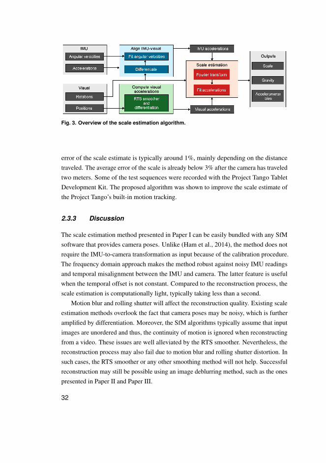
Fig. 3. Overview of the scale estimation algorithm.

error of the scale estimate is typically around 1%, mainly depending on the distancetraveled. The average error of the scale is already below 3% after the camera has traveledtwo meters. Some of the test sequences were recorded with the Project Tango TabletDevelopment Kit. The proposed algorithm was shown to improve the scale estimate ofthe Project Tango’s built-in motion tracking.

2.3.3 Discussion

The scale estimation method presented in Paper I can be easily bundled with any SfMsoftware that provides camera poses. Unlike (Ham et al., 2014), the method does notrequire the IMU-to-camera transformation as input because of the calibration procedure.The frequency domain approach makes the method robust against noisy IMU readingsand temporal misalignment between the IMU and camera. The latter feature is usefulwhen the temporal offset is not constant. Compared to the reconstruction process, thescale estimation is computationally light, typically taking less than a second.

Motion blur and rolling shutter will affect the reconstruction quality. Existing scaleestimation methods overlook the fact that camera poses may be noisy, which is furtheramplified by differentiation. Moreover, the SfM algorithms typically assume that inputimages are unordered and thus, the continuity of motion is ignored when reconstructingfrom a video. These issues are well alleviated by the RTS smoother. Nevertheless, thereconstruction process may also fail due to motion blur and rolling shutter distortion. Insuch cases, the RTS smoother or any other smoothing method will not help. Successfulreconstruction may still be possible using an image deblurring method, such as the onespresented in Paper II and Paper III.

32

Drift is another challenge related to SfM and SLAM. The problem is that the scalemay change over time. Bundle adjustment and loop closure techniques can mitigatethis problem to some extent. To eliminate the scale drift, it was assumed that someparts of the scene remain visible throughout the video. This is a reasonable assumption,for example, when reconstructing an object on a table. A tightly integrated fusion ofvisual and inertial measurements has been shown to reduce the drift in a SLAM system(Mur-Artal & Tardós, 2017b). A similar approach could be used in the SfM pipeline.

33

34

3 Low-light imaging with handheld devices

The exposure of a photograph depends on three variables: exposure time (shutterspeed), ISO value (sensitivity), and aperture. Capturing high-quality photographsunder low-light imaging conditions is a classical problem. Long exposure time isoften required to obtain a sufficient signal-to-noise ratio. The downside is that longexposure can lead to motion blur, for example, due to handshake or scene motion. Onthe other hand, the lack of light can be compensated for by increasing the ISO value.Unfortunately, an analog or digital gain also amplifies the image noise. The last optionis to increase the aperture so that the sensor receives more light. A wider aperture willreduce the depth of field, which can be an advantage or disadvantage depending on thesituation. The effects of different camera settings are illustrated in Fig. 4.

The problems related to low-light imaging affect all cameras but they are mostpronounced in mobile devices, where the camera and optics need to be small andaffordable. A small image sensor is able to capture fewer photons compared to alarge sensor in the same exposure time. To get rich colors, good brightness, and lownoise, the exposure time should be increased. As mentioned, this makes the imagecapture susceptible to motion blur. The problem is emphasized in mobile devices,which are lightweight and difficult to keep steady for long periods. Furthermore,

Fig. 4. The effects of exposure time, ISO value, and aperture (f-stop number). The exposureis the same in all cases but there is a trade-off between image noise, motion blur, and depthof field. Images were captured with Canon EOS 5D Mark IV at 24 mm focal length. The imageon the far right was captured with a stationary camera.

35

smartphone cameras have a fixed aperture. Choosing a wider aperture to improvelow-light performance is therefore not an option.

Optical image stabilization (OIS) has become an essential camera feature in high-endsmartphones. It can reduce motion blur to some extent by physically moving the sensoror lens elements to counteract camera shake. Nevertheless, OIS cannot compensatefor large movements or scene motion. A flash can also be used to improve low lightperformance in some situations. However, the flash has a limited range and often makesthe photograph look unnatural.

Image deblurring and denoising techniques provide another way to improve low-lightphotography. Section 3.1 describes the motion blur model used in Papers II, III, andIV. Section 3.2 gives an overview of existing blind and non-blind image deblurringtechniques. Section 3.3 focuses on inertial-aided deblurring, which is the topic of PapersII and III. Multi-image restoration is discussed in Section 3.4. The section also coversthe problem of joint denoising and deblurring that is addressed in Paper IV.

3.1 Motion blur

Motion blur is often unavoidable when filming in light-limited conditions. It is causedby the relative motion between the camera and the scene during the image exposure. A3D point in the scene is projected to many 2D points on the image sensor, which appearsas motion blur. The blurring process can be modeled with the convolution operation

B = I⊗k+N, (3)

where B and I denote blurry and sharp images, respectively. The blur kernel, alsoknown as the point spread function (PSF), is denoted by k. The symbol ⊗ represents theconvolution operation and N is the additive noise term.

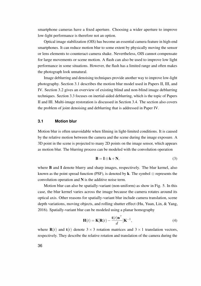
Motion blur can also be spatially-variant (non-uniform) as show in Fig. 5. In thiscase, the blur kernel varies across the image because the camera rotates around itsoptical axis. Other reasons for spatially-variant blur include camera translation, scenedepth variations, moving objects, and rolling shutter effect (Hu, Yuan, Lin, & Yang,2016). Spatially-variant blur can be modeled using a planar homography

H(t) = K[R(t)− t(t)n>

d]K−1, (4)

where R(t) and t(t) denote 3× 3 rotation matrices and 3× 1 translation vectors,respectively. They describe the relative rotation and translation of the camera during the

36

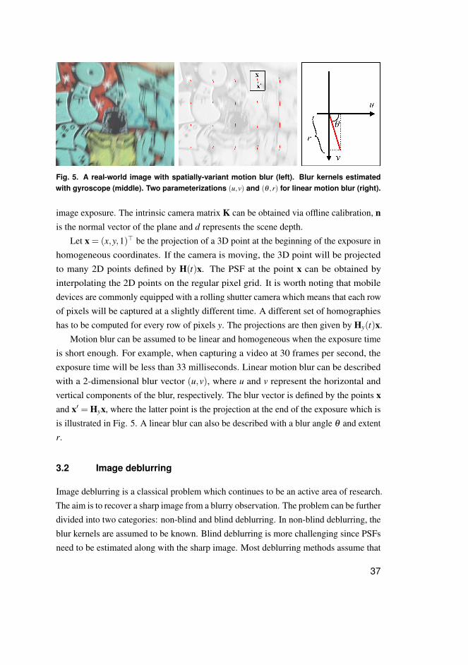
Fig. 5. A real-world image with spatially-variant motion blur (left). Blur kernels estimatedwith gyroscope (middle). Two parameterizations (u,v) and (θ ,r) for linear motion blur (right).

image exposure. The intrinsic camera matrix K can be obtained via offline calibration, nis the normal vector of the plane and d represents the scene depth.

Let x = (x,y,1)> be the projection of a 3D point at the beginning of the exposure inhomogeneous coordinates. If the camera is moving, the 3D point will be projectedto many 2D points defined by H(t)x. The PSF at the point x can be obtained byinterpolating the 2D points on the regular pixel grid. It is worth noting that mobiledevices are commonly equipped with a rolling shutter camera which means that each rowof pixels will be captured at a slightly different time. A different set of homographieshas to be computed for every row of pixels y. The projections are then given by Hy(t)x.

Motion blur can be assumed to be linear and homogeneous when the exposure timeis short enough. For example, when capturing a video at 30 frames per second, theexposure time will be less than 33 milliseconds. Linear motion blur can be describedwith a 2-dimensional blur vector (u,v), where u and v represent the horizontal andvertical components of the blur, respectively. The blur vector is defined by the points xand x′ = Hyx, where the latter point is the projection at the end of the exposure which isis illustrated in Fig. 5. A linear blur can also be described with a blur angle θ and extentr.

3.2 Image deblurring

Image deblurring is a classical problem which continues to be an active area of research.The aim is to recover a sharp image from a blurry observation. The problem can be furtherdivided into two categories: non-blind and blind deblurring. In non-blind deblurring, theblur kernels are assumed to be known. Blind deblurring is more challenging since PSFsneed to be estimated along with the sharp image. Most deblurring methods assume that

37

the blur is spatially-invariant. The problem of image deblurring then reduces to that ofimage deconvolution.

3.2.1 Non-blind deblurring

Non-blind deconvolution is a process of recovering a sharp image I under the assumptionthat blur kernel k is known (See Eq. 3). The simplest approach is to invert the convolutionprocess by inverse filtering. In practice, this will often produce severe visual artifacts,such as ringing near edges. Motion blur PSFs are typically band-limited and non-invertible. Image noise, quantization errors, saturation, and the non-linear cameraresponse curve further complicate the problem (Rajagopalan & Chellappa, 2014). Moreadvanced deconvolution methods aim to reduce ringing artifacts, suppress noise, andimprove computational efficiency.

Most algorithms minimize an energy function consisting of data and regularizationterms. The data term corresponds to the likelihood in probability. It measures thedifference between the convolved sharp image and the blurry image. The L2 -normis a commonly used distance function, which can be written as ‖I⊗k−B‖2. Theregularization term, also known as prior, varies depending on the method. A Gaussianregularizer ‖∇I‖2, for example, enforces the smoothness on image gradients, where ∇

is the gradient operator (Rajagopalan & Chellappa, 2014). Section 3.2.2 provides anoverview of image priors used in recent methods.

Wiener deconvolution (Wiener, 1949) and the Richardson-Lucy method (Lucy, 1974;Richardson, 1972) are traditional approaches that were proposed decades ago. They arestill popular choices due to their computational simplicity and efficiency. Recently, deepnetworks have been used to remove deconvolution artifacts that traditional methodstypically create (Son & Lee, 2017; Wang & Tao, 2018).

Classical deblurring methods often use sparse priors that make the minimizationproblem non-convex. Iteratively reweighted least squares (IRLS) has been used tosolve non-convex deconvolution problems (Joshi, Zitnick, Szeliski, & Kriegman, 2009).More efficient algorithms have also been proposed, such as (Krishnan & Fergus, 2009),which is based on half-quadratic splitting (Geman & Yang, 1995). Many recent classicaldeblurring methods use this type of optimization scheme (Chen, Fang, Wang, & Zhang,2019; Pan, Sun, Pfister, & Yang, 2016; Yan, Ren, Guo, Wang, & Cao, 2017). Thedeconvolution algorithm by Krishnan and Fergus (2009) has also been adapted tospatially-variant deblurring (Whyte, Sivic, Zisserman, & Ponce, 2012).

38

3.2.2 Blind deblurring

Blind deconvolution aims to recover a sharp image I when blur kernel k is unknown.The challenge is that many different pairs of I and k can produce the same blurry imageB. For example, one solution that always satisfies Eq. 3 is the case when k equals deltakernel (no blur) and I = B. Similar to non-blind deconvolution, the energy function tobe minimized typically consists of data and regularization terms. Motion blur PSFs tendto have most elements close to zero. A regularization term, such as ‖k‖2, can be used toenforce the sparsity of the blur kernel.

Classical deblurring methods often use priors that favor natural image statistics. Acommon approach is to assume the sparsity of image gradients (Levin, Weiss, Durand,& Freeman, 2009). The dark channel prior (Pan et al., 2016) is based on the observationthat the smallest pixel value in a local neighborhood is typically less dark when theimage is blurry. The bright channel prior (Yan et al., 2017) is based on a similar ideabut it is better suited for situations where bright pixels dominate the input image. Thelocal maximum gradient prior (Chen et al., 2019) builds upon the observation that themaximum gradient value of a local patch decreases when the image is blurry. Priorsbased on deep networks have also been proposed (L. Li et al., 2018; Zhang, Zuo, Gu, &Zhang, 2017). Some methods are designed for specific image domains, such as text andface images (Lu, Chen, & Chellappa, 2019).

Various learning-based deblurring methods have been proposed recently. Somemethods first estimate blur kernels using a CNN and, thereafter, perform non-blinddeconvolution (Gong et al., 2017; Sun, Cao, Xu, & Ponce, 2015). There are end-to-endapproaches where a network takes a blurry image as input and directly outputs adeblurred image (Gao, Tao, Shen, & Jia, 2019; Kupyn, Budzan, Mykhailych, Mishkin,& Matas, 2018; Nah, Hyun Kim, & Mu Lee, 2017; Tao, Gao, Shen, Wang, & Jia,2018). These methods are especially good at generating perceptually compelling images.Besides producing less deblurring artifacts, they are typically faster than the classicaloptimization-based methods.

In addition to single-image methods, some deblurring approaches utilize stereoimages (Zhou et al., 2019), image bursts (Aittala & Durand, 2018) or videos (Su et al.,2017). Multi-image restoration techniques will be discussed in Section 3.4.

39

3.3 Inertial-aided deblurring

Smartphones and tablet computers are commonly equipped with an IMU. It providesrelatively accurate short-time estimates of the motion of the camera during the imageexposure. Camera rotations can be obtained by integrating angular velocities measuredby a gyroscope. Assuming that the initial velocity of the camera is known, the integrationof accelerometer readings gives the translation. Spatially-variant PSFs can then becomputed using Eq. 4.

Hu et al. (2016) discuss the challenges related to inertial-based blur estimation.Motion blur depends on the scene depth when the camera translates. Depth informationis typically unknown and difficult to estimate from a single image. The IMUs inmobile devices are relatively low quality and noisy. They are mainly designed fortasks such as gaming, that do not require a high-level of accuracy. The integration ofnoisy measurements causes drift, especially when the integration period (exposuretime) is long. Raw acceleration data also includes a gravity component which has to beestimated and removed before integration. Furthermore, there may be an unknown timedelay between inertial and visual measurements.

Despite the aforementioned challenges, inertial measurements have been successfullyused for improving deblurring. Šindelár and Šroubek (2013) implemented an inertial-based deblurring method on a smartphone. They estimate spatially-invariant motion blurusing a gyroscope. Joshi, Kang, Zitnick, and Szeliski (2010) use both the gyroscopeand accelerometer to remove camera shake blur. In the process, they estimate a singledepth value for the scene. Hu et al. (2016) obtain sparse depth information using aphase-based auto-focus of a smartphone camera. They use IMU data as guidance forPSF estimation rather than directly computing the PSFs from the camera motion.

It has been shown that rotation is typically the main cause of motion blur (Park& Levoy, 2014). Translation will have little effect when the scene is sufficiently faraway. Therefore, a common approach is only to estimate the rotation using a gyroscope.Park and Levoy (2014) utilize multiple images and gyroscope measurements. Theyconcluded that non-blind deconvolution using gyroscope readings gives better resultsthan direct alignment and averaging of the input images. Zhang and Hirakawa (2016)modify a conventional blind deblurring framework by including the so-called "IMUfidelity" term to the cost function, which penalizes blur kernels that are not consistentwith gyroscope measurements. The resulting non-convex energy minimization problemis solved with the help of a distance transform.

40

3.3.1 Fast motion deblurring

Paper II proposes a gyro-based deblurring method, referred to as FastGyro, which ismainly designed to improve feature detection and matching in the presence of motionblur. It has been shown that motion blur degrades the performance of traditional featuredetectors and descriptors (Gauglitz, Höllerer, & Turk, 2011). The issue is most apparentin applications that involve a moving camera such as visual odometry, SLAM, and AR.Most deblurring methods are much too computationally expensive to be used in thistype of real-time applications.

FastGyro handles spatially-variant motion blur and rolling shutter distortion inreal-time. The following gives a brief overview of the method. First, the camera rotationsR(t) are computed by integrating gyroscope readings. The PSFs are then estimatedusing Eq. 4 while taking into account the rolling shutter. The scene is assumed to besufficiently far away so that translations t(t) and depth d can be ignored. Motion blur isapproximated to be linear and homogeneous since the exposure time is relatively short(less than 33 ms). The blur is parameterized by angle θ and extent r.

Before deblurring, the gyro-based blur estimates are validated using image data. Ifthere is both rotation and translation, the image may appear sharp while the gyroscopemeasures rotation. The purpose of blur validation is to avoid deblurring an image that isalready sharp. The blur estimate is considered incorrect if the gradient magnitude alongthe estimated motion direction θ exceeds a certain threshold. Then, the image is notdeblurred in order to avoid artifacts.

After the blur estimation and validation, the image is divided into smaller blockswhich are deblurred separately using Wiener deconvolution in the spatial domain. Thespatial domain representation has advantages over the conventional frequency domainapproach. Most importantly, the deconvolution kernels can be computed offline, enablingfast GPU implementation and real-time performance. It takes around 17 millisecondsto deblur a grayscale image with a resolution of 1920 x 1080 pixels on an NVIDIAGeForce GTX 1080 GPU.

The experiments were conducted using the Difference of Gaussian (DoG) detector(Lowe et al., 1999) and SIFT descriptor (Lowe, 2004). Fig. 6 demonstrates keypointdetection and deblurring on synthetically blurred images. FastGyro improves therepeatability, meaning the corresponding scene regions are better identified fromthe two images. The experiments in Paper II show that FastGyro also increases thenumber of detected keypoints and improves the localization accuracy of the detector.

41

Moreover, these improvements will lead to more accurate and complete reconstructionswhen used in the application of image-based 3D reconstruction. Fig. 7 shows thedeblurring performance on a real-world image with spatially-variant motion blur. Someringing artifacts can be seen in the output which is a common issue among non-blinddeconvolution methods.

Fig. 6. Keypoint detection without deblurring (left). Deblurring with FastGyro (right) in-creases the number of correspondences and improves the localization accuracy of the de-tector. A fixed number of 100 DoG keypoints was detected from each image.

3.3.2 Deblurring with deep networks

Paper III proposes a gyroscope-aided deblurring method called DeepGyro. It is the firstapproach incorporating gyroscope measurements into a CNN. Non-blind deconvolutionmethods, such as FastGyro in Paper II, often produce deblurring artifacts. The problemis made worse by the fact that gyro-based blur estimates may be inaccurate. This can becaused, for example, by noisy IMU readings, temporal misalignment of the IMU andcamera, and translation when the scene is close. DeepGyro utilizes both image data anda gyroscope to overcome these limitations, as demonstrated in Fig. 7.

Fig. 7. A real-world image with spatially-variant motion blur (left). Deblurred images pro-duced by FastGyro (middle) and DeepGyro (right).

42

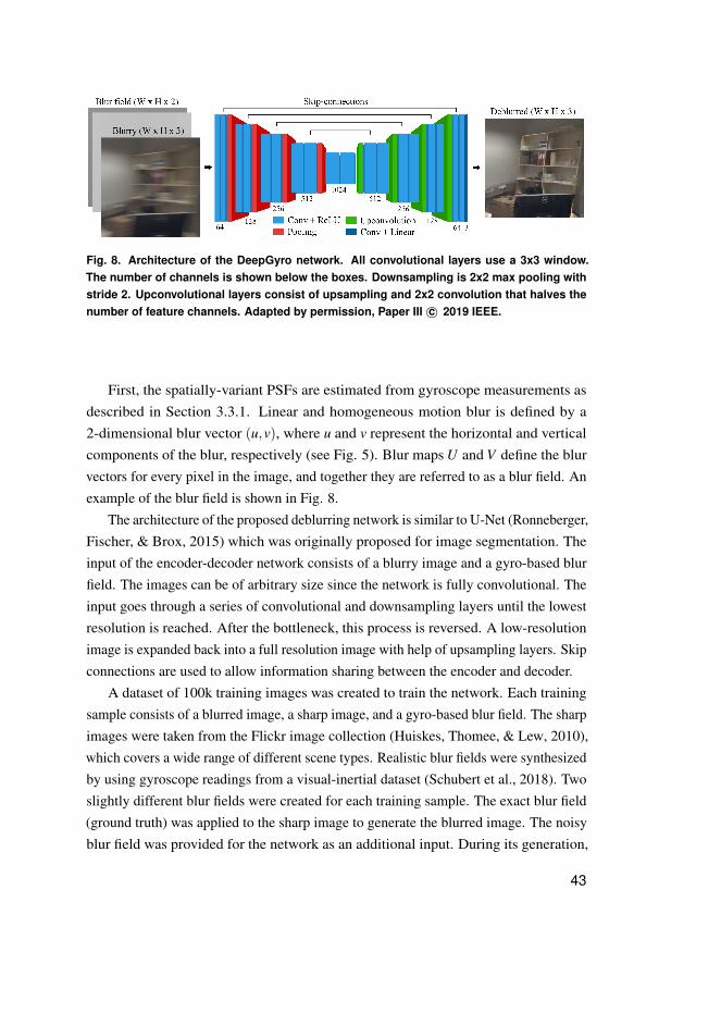
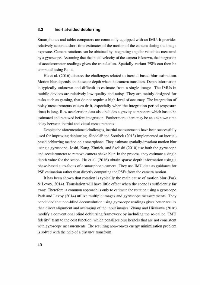
Fig. 8. Architecture of the DeepGyro network. All convolutional layers use a 3x3 window.The number of channels is shown below the boxes. Downsampling is 2x2 max pooling withstride 2. Upconvolutional layers consist of upsampling and 2x2 convolution that halves thenumber of feature channels. Adapted by permission, Paper III c© 2019 IEEE.

First, the spatially-variant PSFs are estimated from gyroscope measurements asdescribed in Section 3.3.1. Linear and homogeneous motion blur is defined by a2-dimensional blur vector (u,v), where u and v represent the horizontal and verticalcomponents of the blur, respectively (see Fig. 5). Blur maps U and V define the blurvectors for every pixel in the image, and together they are referred to as a blur field. Anexample of the blur field is shown in Fig. 8.

The architecture of the proposed deblurring network is similar to U-Net (Ronneberger,Fischer, & Brox, 2015) which was originally proposed for image segmentation. Theinput of the encoder-decoder network consists of a blurry image and a gyro-based blurfield. The images can be of arbitrary size since the network is fully convolutional. Theinput goes through a series of convolutional and downsampling layers until the lowestresolution is reached. After the bottleneck, this process is reversed. A low-resolutionimage is expanded back into a full resolution image with help of upsampling layers. Skipconnections are used to allow information sharing between the encoder and decoder.

A dataset of 100k training images was created to train the network. Each trainingsample consists of a blurred image, a sharp image, and a gyro-based blur field. The sharpimages were taken from the Flickr image collection (Huiskes, Thomee, & Lew, 2010),which covers a wide range of different scene types. Realistic blur fields were synthesizedby using gyroscope readings from a visual-inertial dataset (Schubert et al., 2018). Twoslightly different blur fields were created for each training sample. The exact blur field(ground truth) was applied to the sharp image to generate the blurred image. The noisyblur field was provided for the network as an additional input. During its generation,

43

the defects of gyro-based blur estimation, including the temporal misalignment, weremodeled.

3.3.3 Discussion

The main advantage of FastGyro and DeepGyro is that they run in real-time, unlike mostdeblurring methods. FastGyro is considerably faster than DeepGyro but it producesmore deblurring artifacts, as evident in Fig. 7. In some applications, minor artifacts maybe acceptable. For example, in image-based 3D reconstruction, feature matches that arenot consistent with the epipolar geometry can effectively be removed using RANSAC.DeepGyro produces visually more appealing images, which is an important feature inapplications such as video deblurring.

Both methods assume that motion blur is only caused by the rotation of the camera.This is true in many cases, however, the translation will have some effect if the scene isclose to the camera. DeepGyro addresses this indirectly by assuming that gyro-basedblur estimates are imperfect. That is, the network is trained with imperfect blur kernels.It can be noted that blur is expected to vary smoothly across the image. This may not bea valid assumption, for example, when there are significant depth variations in the sceneor when the scene is dynamic.

DeepGyro has an important property in that it does not attempt to deblur imageregions which are already sharp. This is useful, for example, when the camera is trackinga moving object and only the background is blurry. On the other hand, the scene motioncannot be observed with an IMU. Therefore, the regions that are blurry due to scenemotion are likely to remain blurry.

Motion blur is approximately linear when the exposure time is relatively short (e.g.,when capturing a video). This assumption is reasonable in applications such as SLAMand AR that would benefit from real-time deblurring. The handling of more complexmotion blur is nevertheless essential in long exposure photography. Extending FastGyroand DeepGyro for longer exposures is an exciting direction for future research.

3.4 Multi-image restoration

Conventional deblurring and denoising methods are limited by the information in asingle image. Multi-image approaches combine information from multiple images.Some methods use special hardware such as a stereo camera. Zhou et al. (2019) proposed

44

a CNN for stereo image deblurring. They show that depth information obtained from thestereo images is useful for estimating spatially varying blur kernels. Moreover, themethod takes advantage of the fact that individual images may be blurred differently.

Ben-Ezra and Nayar (2003) use a hybrid camera system for motion deblurring. Theprimary camera captures a blurry high-resolution image and the secondary cameracaptures a low-resolution video sequence with high temporal resolution. An optical flowbased method is used to recover the blur PSF from the video sequence. This is followedby a non-blind deconvolution step to recover the sharp image. The idea of using a hybridcamera for motion deblurring was later extended to videos with spatially-variant blur(Tai, Du, Brown, & Lin, 2008).

Shen, Yan, Xu, Ma, and Jia (2015) proposed a general multi-spectral imagerestoration framework. The input can be, for example, a pair of RGB and near infrared(NIR) images. A guidance image (NIR image) is used to recover a better version ofthe RGB image. Guided image filtering (He, Sun, & Tang, 2012) uses a guidanceimage to preserve edges while smoothing. The guided filter can be applied to a varietyof applications, including noise reduction, detail enhancement, image matting, hazeremoval, and joint upsampling. Zhuo, Guo, and Sim (2010) use a pair of flash and non-flash images for image deblurring. The so-called flash gradient constraint encouragesthe gradients of the estimated sharp image to be close to those in the flash image.

Many current mobile devices can be programmed to capture rapid bursts of images.Various multi-image deblurring and denoising methods have been proposed recently.Aittala and Durand (2018) capture a burst of long exposure images and recover a sharpand noise-free image using a neural network. They propose a CNN architecture thattreats all input images in an order-independent manner. Su et al. (2017) address theproblem of video deblurring. Information across neighboring frames is accumulatedwith a CNN that is trained end-to-end. Mildenhall et al. (2018) denoise bursts of imagescaptured with a hand-held camera. They use a CNN to predict spatially varying kernelsthat can both align and denoise the images.

The challenge with multi-image methods is that input images are often misaligned.The alignment of blurry or noisy images can be challenging, especially when the sceneis dynamic. Fast-moving objects can also disappear from the view if the capturingtakes too long. Sometimes image details and colors may be permanently lost. This canhappen, for example, when the image is over or under-exposed.

Some methods aim to recover a high-quality image using a pair of short and longexposure images (Jia, Sun, Tang, & Shum, 2004; Lee, Park, & Hwang, 2012; H. Li,

45

Zhang, Sun, & Gong, 2014; Tai, Jia, & Tang, 2005; Whyte et al., 2012; Yuan, Sun,Quan, & Shum, 2007). One approach is to transfer the colors from a blurry longexposure image to a short exposure image (Jia et al., 2004; Tai et al., 2005). However,these methods do not consider that the short exposure image may be noisy. An imagedenoising algorithm is therefore needed to obtain a noise-free image. In denoising, thereis often a compromise between detail preservation and noise removal.

Yuan et al. (2007) exploit a denoised image to recover the blur kernel. The so-calledresidual deconvolution is then used to iteratively estimate the residual image that is to beadded to the denoised image. The method was later extended to handle spatially-variantmotion blur (Whyte et al., 2012). Lee et al. (2012) construct an edge map from a slightlydenoised image. The blur kernel is estimated using edge regions only defined by theedge map. The sharp image is recovered with a deconvolution method while imposing ahyper-Laplacian prior on the image gradients. H. Li et al. (2014) estimate a blur kerneland sharp image simultaneously using an alternating optimization scheme and the IRLSmethod.

3.4.1 Joint denoising and deblurring

Paper IV proposes a joint denoising and deblurring method referred to as LSD2 (Long-Short Denoising and Deblurring). As previously discussed, it is challenging to capturesatisfactory photographs with handheld smartphone cameras in low light imagingconditions. To get rich colors, good brightness and low noise levels, one should chooselong exposure with a low ISO setting. However, this will introduce motion blur if thecamera or scene is moving. On the other hand, short exposure with a high ISO settingwill produce sharp but noisy images.

LSD2 avoids the unsatisfactory trade-off between the short and long exposuresettings. The method fuses a pair of short and long exposure images into a singlehigh-quality image. Fig. 9 shows an image pair captured with a Google Pixel 3smartphone. The short exposure image has been normalized so that its intensity matchesthe blurry image for visualization. Note that the input images are slightly misalignedeven though they are captured immediately one after the other. The images are jointlydenoised and deblurred by a deep CNN.

The LSD2 network has the same architecture as the DeepGyro in Fig. 8. The networkwas trained using a large volume of synthetic short and long exposure images that weregenerated from regular high-quality photographs. The imaging effects modeled include

46

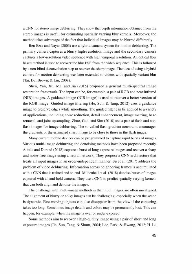
Fig. 9. Joint denoising and deblurring with LSD2. From left to right: short exposure image(noisy), long exposure image (blurry), and LSD2 output (sharp and noise-free).

motion blur, image noise, spatial misalignment, color distortion, and saturation. Thenetwork was also fine-tuned using real pairs of short and long exposure images. For thispurpose, various scenes were captured with a static camera. The long exposure image ineach pair was the sharp target for the network. Blurred inputs were obtained by addingsynthetic blur to the sharp images.

Besides the problems of noise and blur, camera sensors have a limited dynamicrange. Even if the camera was perfectly still, it might not be able to capture the fulldynamic range of the scene with a single exposure. Thus, details are typically lost eitherin dark shadows or bright highlights. This problem can be solved using an exposurefusion algorithm, such as Prabhakar, Srikar, and Babu (2017), that takes a pair of shortand long exposure images as input. However, the existing methods generally assumethat input images are neither blurry nor misaligned.

LSD2 provides a solution to the problem above. The LSD2 output is aligned with theshort exposure image which makes them suitable inputs for exposure fusion. To this end,an exposure fusion network was trained that takes the short exposure image and theLSD2 output as input. The network produces images with better colors and brightnessthan a single-exposure smartphone image. The exposure fusion in the presence ofmotion blur is demonstrated in Fig. 10. The input pair was captured with an NVIDIAShield tablet. Notice the recovery of details in the under and over-exposed regions in thewindow area.

47

Fig. 10. Exposure fusion with LSD2. From left to right: short exposure image (noisy), longexposure image (blurry), and tone mapped LSD2 output.

3.4.2 Discussion

The LSD2 method in Paper IV has several advantages over existing approaches thatutilize short and long exposure image pairs (Lee et al., 2012; H. Li et al., 2014;Whyte et al., 2012; Yuan et al., 2007). Apart from Whyte et al. (2012), these methodscannot handle spatially-variant blur. Furthermore, the input images need to be aligned(manually), which limits their practical use. For example, Yuan et al. (2007) producessevere artifacts when input images are misaligned. LSD2 does not rely on existingdenoising algorithms unlike some previous works (Lee et al., 2012; Whyte et al., 2012;Yuan et al., 2007). Moreover, LSD2 does not have any tunable parameters and performssurprisingly well on dynamic scenes, even though it was trained only with static scenes.The dynamic scene performance is assessed in Fig. 11. Some ghosting artifacts can beseen around moving objects but including images with synthetic scene motion to thetraining set might resolve the issue. Moreover, it may also be beneficial to considercamera translation and scene depth when generating training data.

On some devices, it may not be possible to capture image bursts without a significanttime delay between the images. This would make the misalignment of the images moresevere. One solution is to pre-align the images using an IMU. Thus, the problem of jointdenoising and deblurring would become easier as the network would not have to learnimage alignment. Furthermore, the IMU could provide valuable information about scenemotion, although it does not directly help to align dynamic scenes.

More realistic noise models have been recently proposed to improve learning-baseddenoising methods (Brooks et al., 2019; Jaroensri, Biscarrat, Aittala, & Durand, 2019).The LSD2 network was fine-tuned with real noisy images, which avoided the need forsuch models. However, the fine-tuning step may become less critical if these types ofmethods are used.

48

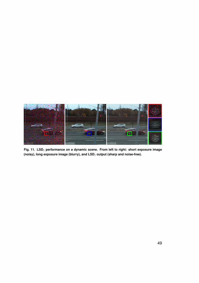
Fig. 11. LSD2 performance on a dynamic scene. From left to right: short exposure image(noisy), long exposure image (blurry), and LSD2 output (sharp and noise-free).

49

50

4 Multi-aperture imaging

A multi-aperture camera refers to an imaging device that contains more than one cameraunit. Terms such as "array camera", "multi-camera" and "multi-sensor camera" are alsoused. An example of a four-aperture camera is shown in Fig. 12. This particular cameraproduces four sub-images that need to be fused into a single RGB image. In general, themain challenge of multi-aperture imaging arises from the fact that each camera unit hasa slightly different viewpoint. Consequently, the sub-images may be misaligned due toparallax. A direct fusion without parallax correction can lead to severe artifacts, asdemonstrated in Fig. 13. The problem can be solved by remapping the pixels in thesub-images into a reference image. In practice, this requires finding the correspondingpixels from each image, which is known as stereo matching.

4.1 Advantages of multi-aperture imaging

Multi-aperture cameras have several advantages over traditional single-aperture cameras.The thickness of the camera is closely related to the image quality the camera produces;cameras equipped with larger image sensors typically produce better images. However,the increase in sensor size will also increase the height of the optics. This is particularlyproblematic in mobile devices in which low-profile cameras are needed. A multi-aperturecamera solves this problem by using a combination of smaller sensors, each having

Fig. 12. Image sensing arrangement of the four-aperture camera. In this camera, three ofthe camera units are equipped with red, green and blue color filters. The fourth camera unitcaptures the luminance. Reprinted by permission from Springer Nature Customer ServiceCentre GmbH: Springer MACHINE VISION AND APPLICATIONS, Paper V c© 2016.

51

dedicated optics with reduced optical height (Kolehmainen, Rytivaara, Tokkonen,Mäkelä, & Ojala, 2008).

Most smartphone cameras do not have an optical zoom as they use fixed focal lengthlenses. In a multi-aperture camera, the lenses can have different focal lengths to enablezoom (Tallon, 2016). Another disadvantage of conventional smartphone cameras is thatthey cannot produce images with shallow depth of field due to the small aperture. Allobjects in the scene are mostly in focus no matter what is their distance from the camera.For artistic purposes, it may be desirable that only the object of interest is in focus. Thisis demonstrated in Fig. 4. The same effect can be synthesized by utilizing the depthinformation estimated with multiple cameras.

Another problem with smartphone cameras is that their dynamic range is typicallyquite limited. Individual pixels are tiny due to the small sensor size and high pixel count.Therefore, the pixels will hit the saturation point after receiving just a small amount oflight. With multiple sensors, the effective size of each pixel increases, which improvesthe dynamic range (Tallon, 2016). The camera units can also have different exposuresettings to further improve the dynamic range.

A multi-aperture camera can include both color and monochrome cameras. Amonochrome camera responds to all wavelengths of light and therefore has better lightefficiency than a color camera. This is beneficial, especially when capturing images atlow light conditions (Jeon et al., 2016).

Existing cameras commonly use a Bayer filter to create a color image. In Bayerfilter cameras, the adjacent pixels measure the light intensity of different color bands.The problem is that neighboring pixels may interact. A phenomenon known as cross-talk occurs when photons received by one pixel are falsely sensed by other pixelsaround it. The most noticeable consequence of cross-talk is the desaturation of color(Hirakawa, 2008). Furthermore, the demosaicing of a Bayer pattern image can introduceinterpolation artifacts (Holloway, Mitra, Koppal, & Veeraraghavan, 2014). The multi-aperture camera in Fig. 12 avoids these problems since three of the cameras onlymeasure a single spectral color. Demosaicing is therefore not needed.

Chromatic aberration is a type of distortion in which a lens fails to focus differentwavelengths of light to the same point on the image sensor (Korneliussen & Hirakawa,2014). This occurs because lens material refracts different wavelengths of light atdifferent angles. The effect can be seen as colored and blurred edges, especially alongboundaries that separate dark and bright parts of the image. The multi-aperture camerain Fig. 12 does not suffer from chromatic aberration, assuming that the camera units

52

Fig. 13. Result of image fusion without and with parallax correction. (a) Red, green, blue andluminance images. (b) Direct fusion results in major color artifacts. (c) Fused image afterthe parallax correction.

have been calibrated for different wavebands. The lenses can also be simpler becausethe chromatic aberration is less of a problem when designing the optics. Furthermore, asimpler design usually leads to lower manufacturing costs.

4.2 Existing multi-aperture cameras

Multi-aperture cameras have become increasingly common in smartphones. The lensesof individual camera units often have different focal lengths. A wide-angle lens is afairly standard feature on high-end smartphones. Some devices, such as the AppleiPhone 11 Pro, include an ultra-wide lens. There are smartphones with optical zoomingcapabilities, such as the Huawei P40 Pro which has a camera with 5x optical zoom. Dueto space restrictions, the camera is placed sideways inside the device. A mirror is thenused to point the camera to the backward direction.

Some high-end smartphones include a time-of-flight (ToF) camera. It can providedepth information by measuring the time difference (or phase difference) between theemitted and received (infrared) light. The resolution of a ToF camera is typically verylow. However, it can be used to confirm and fine-tune the initial depth map generated byconventional cameras. This can help to create a more convincing synthetically refocusedimage, among other applications.

The Nokia 9 PureView smartphone uses a combination of monochrome and colorcameras. It captures five images simultaneously and computationally fuses them. Similartechnology is used in the Light L16 camera, which comprises of 16 color cameras(Tallon, 2016). The lenses have different focal lengths to enable zoom. The final image is

53

constructed by fusing 10 simultaneously captured images. As with other multi-aperturecameras, the depth of field can be adjusted post-capture based on the estimated depth.Furthermore, the Light L16 camera naturally allows an increased dynamic range sincecameras can have different exposures.

Holloway et al. (2014) build a prototype four-aperture camera, which is similar tothe one shown in Fig. 12. They used monochrome Point Grey Flea3 machine visioncameras equipped with different color filters. The absence of demosaicing artifactsand improved low light performance was demonstrated by comparing to the Flea3color camera. PiCam (Pelican Imaging Camera-Array) is a multi-aperture camera thatconsists of 4 × 4 array of cameras (Venkataraman et al., 2013). PiCam is similar to thefour-aperture camera in the sense that each camera has dedicated optics and a colorfilter. The final image is constructed from the sub-images using stereo matching andsuper-resolution techniques.

4.3 Stereo matching

Stereo matching is an old and widely studied problem in computer vision. The problemis related to image-based 3D reconstruction which was discussed in Chapter 2. Theobjective is to find corresponding points between two images captured from differentviewpoints. In stereo matching, the cameras are usually calibrated so that their relativepositions and orientations are known. Correspondences are typically estimated forevery pixel in the image. Stereo matching is needed when fusing images taken with amulti-aperture camera. The corresponding pixels are remapped to a reference image toalign the images.

The correspondence problem can be simplified by carefully aligning the camerasso that there is only a horizontal (or vertical) translation between the cameras. If thecameras are perfectly aligned, the corresponding points will be on the same pixel rows.Their horizontal coordinate difference is referred to as disparity. The result of stereomatching is commonly represented by a disparity map, which shows the disparities(correspondences) for every pixel in the image. Disparities are large if the object isclose to the camera, as can be observed in Fig. 14. This is because disparity is inverselyproportional to the depth of the scene point.

Perfect camera alignment is often difficult and impractical. Alternatively, a processcalled image rectification can be used (Szeliski, 2010). The rectification transforms theimages so that conjugate epipolar lines become collinear and parallel to the horizontal

54

image axis. The rectified images can be considered as if they were captured usingperfectly aligned cameras.

Disparity estimation can often be improved by using more than two images. Therobustness against noise and radiometric differences increases when multiple images arematched simultaneously. Arranging cameras both horizontally and vertically can resolveambiguities that are common in a two-view case. For example, it is problematic tomatch points that are on an edge parallel to the baseline. A multi-view camera systemalso provides more information about occlusions. A point may be occluded in one of theviews but matching may still be possible using the other views.

4.3.1 Matching costs

A matching cost is needed in order to measure the similarity of image locations. It istypically computed at each pixel for every candidate disparity in a given range. Thesimplest way to measure whether two pixels are similar is by taking their absoluteor squared intensity difference. Alternatively, the differences can be summed over afixed window to improve robustness against noise. For example, the sum of absolutedifferences (SAD) is used in the PiCam camera array (Venkataraman et al., 2013) tomatch images that are captured using similar color filters.

The problem with conventional matching costs is that they perform poorly in thepresence of radiometric differences such as lighting and exposure changes. Similarproblems arise when matching images captured with different color filters. The inputimages in Fig. 13 were captured with a camera system representing the four-aperturecamera. Notice that corresponding pixels can have very different intensities due to thecolor filters, which complicates the matching process.

A comprehensive evaluation of 15 different matching costs (Hirschmüller &Scharstein, 2008) concluded that the Census transform (Zabih & Woodfill, 1994)has the best overall performance when matching images with radiometric differences.The pixelwise mutual information (MI) (Hirschmüller, 2008; Kim, Kolmogorov, &Zabih, 2003) also performed well, especially in case of strong image noise. Whenradiometric differences were not too severe, background subtraction by bilateral filtering(BilSub) (Ansar, Castano, & Matthies, 2004) provided good results.

Normalized cross-correlation (NCC) is often used to match images with radiometricvariations. Similar to other window-based costs (e.g. SAD), it may suffer from theflattening effect near the object boundaries. To combat this weakness, Heo, Lee, and Lee

55

(2011) proposed an adaptive normalized cross-correlation (ANCC). Robust selectivenormalized cross correlation (RSNCC) was proposed by Shen, Xu, Zhang, and Jia(2014) to handle gradient and color variations and structural inconsistency caused bynoise, shadows, and reflections.

The SAD cost has been combined with the sum of informative edges (SIE) costto match monochrome and color images (Jeon et al., 2016). A dense adaptive self-correlation (DASC) descriptor was proposed to match multi-modal and multi-spectralimage pairs (Kim et al., 2015). The matching performance was demonstrated on RGBand near-infrared (NIR) images, flash and no-flash images, and image pairs taken withdifferent exposures. Pinggera, Breckon, and Bischof (2012) matched RGB and thermalimages using dense gradient features based on the Histograms of Oriented Gradient(HOG) descriptor.

Holloway et al. (2014) proposed a matching cost for a four-aperture camera. Theircross-channel normalized gradient (CCNG) cost is based on aligning normalizedgradients (edges) across color channels. A smoothness cost is added to improve theperformance in textureless regions. Their experiments show that CCNG outperforms thewindow-based MI in terms of depth map quality.

Recently, CNNs have been utilized for matching cost computation. Žbontar andLeCun (2016) train a deep siamese network to predict the similarity between imagepatches. Shaked and Wolf (2017) compute matching costs with a highway network basedon multilevel weighted residual shortcuts. Aguilera, Aguilera, Sappa, Aguilera, andToledo (2016) compare the similarity of cross-spectral image patches. They experimentwith three different CNN architectures, each trained using RGB and NIR images. Somearchitectures are shown to generalize between different cross-spectral domains.

4.3.2 Disparity estimation

Disparity estimation methods aim to find correct disparities for every pixel in theimage based on the matching costs. The algorithms can be classified into two majorcategories: local and global methods. Local methods estimate disparities independentlyfor each pixel. That is, a disparity of a pixel does not depend on the disparities ofthe neighboring pixels. Global methods take into account all matching costs withinthe image. They estimate disparities for every pixel at the same time using energyminimization techniques. An exact classification to local and global methods can bedifficult because there are methods that have characteristics from both categories.

56

Local methods

In local methods, the disparity computation at a given pixel depends only on the intensityvalues within a finite window. For example, when using the SSD matching cost, thepixel-wise squared differences are summed over a fixed window. A matching cost istypically computed at each pixel for all candidate disparities in a given disparity range.Computing the final disparities is trivial when using a local method. The disparityassociated with the minimum cost is chosen as the best match.

The selection of an appropriate window size is critical. The window should be largeenough so that it contains enough intensity variations for reliable matching. A largewindow may result in undesired smoothing of discontinuities. This is due to the implicitassumption that all pixels within the window have similar disparities. On the other hand,too small of a window typically results in a noisy disparity map.

Various approaches have been proposed to address the problems of fixed-sizewindows. The fast variable window method by Veksler (2003) finds a suitable windowsize from a specified range. Yoon and Kweon (2006) adjust the weights within thewindow based on color similarity and spatial distance. Segmentation-based weightinghas also been proposed (Tombari, Mattoccia, & Di Stefano, 2007). The guided imagefilter (He et al., 2012) has been adapted to stereo matching. According to Hosni, Bleyer,and Gelautz (2013), the guided filter has the best overall performance in terms ofdisparity map quality and computational efficiency. Zhu and Yan (2017) modify theguided filter with adaptive rectangular support windows (ARSW) instead of using afixed window.

Global methods

Many computer vision problems can be formulated in terms of energy minimization.In stereo matching, the aim is to assign disparities in such a way that a global energyfunction is minimized. The energy function usually consists of a data and a smoothnessterm. The data term can be expressed as the sum of all matching costs given a certaindisparity map. The motivation behind a smoothness term is that disparities tend to varysmoothly across neighboring pixels, except at object boundaries. The general idea is tofavor smooth disparity maps by assigning higher penalties for pairs of neighboringpixels when their disparities differ.

57

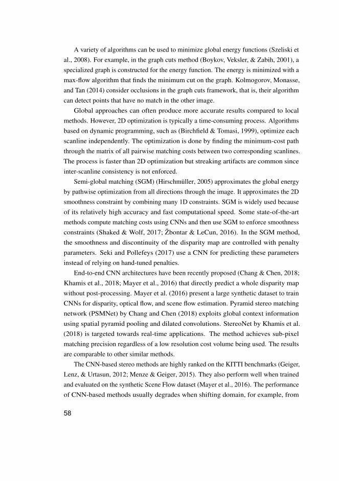
A variety of algorithms can be used to minimize global energy functions (Szeliski etal., 2008). For example, in the graph cuts method (Boykov, Veksler, & Zabih, 2001), aspecialized graph is constructed for the energy function. The energy is minimized with amax-flow algorithm that finds the minimum cut on the graph. Kolmogorov, Monasse,and Tan (2014) consider occlusions in the graph cuts framework, that is, their algorithmcan detect points that have no match in the other image.

Global approaches can often produce more accurate results compared to localmethods. However, 2D optimization is typically a time-consuming process. Algorithmsbased on dynamic programming, such as (Birchfield & Tomasi, 1999), optimize eachscanline independently. The optimization is done by finding the minimum-cost paththrough the matrix of all pairwise matching costs between two corresponding scanlines.The process is faster than 2D optimization but streaking artifacts are common sinceinter-scanline consistency is not enforced.

Semi-global matching (SGM) (Hirschmüller, 2005) approximates the global energyby pathwise optimization from all directions through the image. It approximates the 2Dsmoothness constraint by combining many 1D constraints. SGM is widely used becauseof its relatively high accuracy and fast computational speed. Some state-of-the-artmethods compute matching costs using CNNs and then use SGM to enforce smoothnessconstraints (Shaked & Wolf, 2017; Žbontar & LeCun, 2016). In the SGM method,the smoothness and discontinuity of the disparity map are controlled with penaltyparameters. Seki and Pollefeys (2017) use a CNN for predicting these parametersinstead of relying on hand-tuned penalties.

End-to-end CNN architectures have been recently proposed (Chang & Chen, 2018;Khamis et al., 2018; Mayer et al., 2016) that directly predict a whole disparity mapwithout post-processing. Mayer et al. (2016) present a large synthetic dataset to trainCNNs for disparity, optical flow, and scene flow estimation. Pyramid stereo matchingnetwork (PSMNet) by Chang and Chen (2018) exploits global context informationusing spatial pyramid pooling and dilated convolutions. StereoNet by Khamis et al.(2018) is targeted towards real-time applications. The method achieves sub-pixelmatching precision regardless of a low resolution cost volume being used. The resultsare comparable to other similar methods.

The CNN-based stereo methods are highly ranked on the KITTI benchmarks (Geiger,Lenz, & Urtasun, 2012; Menze & Geiger, 2015). They also perform well when trainedand evaluated on the synthetic Scene Flow dataset (Mayer et al., 2016). The performanceof CNN-based methods usually degrades when shifting domain, for example, from

58

synthetic training images to real-world images. Therefore, the networks are typicallyfine-tuned in the target environment. Classical approaches, such as the method byTaniai, Matsushita, Sato, and Naemura (2018), which is based on graph cuts, are stillcompetitive with deep networks when not enough fine-tuning data is available. This isthe case, for example, with Middlebury stereo benchmarks (Scharstein et al., 2014) thatdo not include a large number of training images.

4.4 Parallax correction in a multi-aperture camera

Paper V proposes an image fusion algorithm for a four-aperture camera. One possibleconfiguration of cameras is shown in Fig. 12. The algorithm corrects the parallax errorbetween the input images and fuses them into a single RGB image. This is done usinga disparity map that is estimated from the images. An important detail is that eachcamera unit measures a different region of the visible color spectrum. This design hasmany advantages as discussed in Section 4.1. Nevertheless, the radiometric differencesbetween the images also make the disparity estimation more challenging.

The image captured with a green color filter is chosen as the reference image. Adisparity map defines the corresponding pixels between the green and red channels. Itwould be straightforward to match each image pair independently. However, such anapproach would not utilize the full potential of multiple views. Instead, the matchingcosts are combined over different images using trifocal tensors and point transfer(Section 2.1.2). The first tensor provides the position of the point in the blue image givena candidate disparity. Similarly, the second tensor relates the disparities to the luminanceimage. Trifocal tensors are computed offline after rectifying the green and red channels.

Paper V compares two alternative matching costs: mutual information and Censustransform. Both costs are known to be robust against radiometric differences. Fur-thermore, a novel luminance cost is added to take advantage of the luminance image.The paper compares two popular disparity estimation methods: graph cuts (GC) andsemi-global matching (SGM). After the disparity estimation, the red and blue channelsare remapped (warped) to the green channel. An RGB image is then constructed bycombining the color channels. The luminance image can also be remapped to improvethe signal-to-noise ratio.

Figures 13 and 14 show the results of image fusion for two different scenes.According to the experiments, SGM with Census transform gave the best overallperformance. The quality of the fused images was near the reference RGB images. A

59

Fig. 14. Post-capture refocusing after image fusion. (a) A disparity map computed fromthe sub-images. (b) A fused image where everything is in focus. (c) A synthetically blurredimage that simulates shallow depth of field. (d) Enlarged image patches.

close inspection of the fused images revealed small color errors, typically found nearthe object boundaries. Interestingly, the errors in the disparity map do not necessarilypropagate to the fused image. For example, incorrect disparities will not cause artifactsif the image region is uniform.

Synthetic refocusing is demonstrated in Fig. 14. The amount of blur that is added toeach pixel depends on how far the corresponding 3D point is from the focal plane. Inthis example, the focal plane is defined to be at the same depth as the flower. It canbe observed that the quality of the depth of field effect is relatively good. Some areasaround the flower are unrealistically blurred due to small inaccuracies in the disparitymap. The quality of the effect highly depends on the accuracy of the disparity map.

4.5 Discussion

The experiments in Paper V did not reveal all the advantages of an actual multi-aperturecamera because test images were captured with a traditional Bayer filter camera.As discussed in Section 4.1, this type of camera may suffer from color cross-talk,demosaicing artifacts, and chromatic aberration. This was not a problem since Paper Vmainly focuses on disparity estimation and image fusion rather than improvements inimage quality. After all, the disparity estimation plays an important role in the quality ofthe final image.

One challenge of a multi-aperture camera is that some parts of the scene maynot be visible in all cameras. The severity of the problem depends on the baselineof the cameras and scene depth. The implementation presented in Paper V does not

60

include occlusion handling, which explains why color artifacts are typically foundnear object boundaries. Occlusion detection and filling would increase the quality ofthe fused images. The missing color values could be filled, for example, with recentlearning-based inpainting (Xiong et al., 2019) or colorization (He, Chen, Liao, Sander,& Yuan, 2018) methods.

Even though the proposed algorithm was designed for a particular multi-aperturecamera, a similar approach could be used in other multi-spectral matching problems.The configuration of the cameras can be chosen freely since the algorithm utilizestrifocal tensors. Furthermore, one could easily add more cameras without significantlyincreasing the computation time.

Promising results have been obtained with CNN-based stereo methods as discussed inSection 4.3.2. Applying the existing pre-trained networks directly to this problem wouldlikely yield poor results due to the known generalization issues of current approaches.Furthermore, the radiometric differences that need to be handled in this problem are veryspecific. Nevertheless, training a CNN-based matching cost or an end-to-end networkfor image fusion would be an interesting direction for future research.

61

62

5 Summary and conclusion

This thesis has presented novel algorithms for improving image-based 3D reconstructionand mobile imaging which take advantage of the features of current mobile devices.This includes the use of an IMU for scale estimation (Paper I) and image deblurring(Papers II-III). Many devices can be programmed to capture rapid bursts of images withdifferent exposure times. This enables the development of joint image denoising anddeblurring techniques (Paper IV). Equipping the device with multiple camera units canimprove image quality and camera features. An image fusion algorithm (Paper V) is anessential component in the so-called multi-aperture camera.

The scale ambiguity is a well-known limitation of image-based 3D reconstruction.The reconstruction is only possible up to a scale when using a monocular camera. PaperI proposed an inertial-based scale estimation that recovers the absolute scale of thereconstruction. The method outperforms the state-of-the-art method (Ham et al., 2015)and achieves an average scale error of 1%. The camera-IMU calibration process allowseasy integration with existing reconstruction software. The scale estimation is performedin the frequency domain to increase the robustness against inaccurate sensor timestampsand noisy IMU readings. The algorithm can cope with noisy camera pose estimates,typically caused by motion blur and rolling shutter distortion.

Motion blur compromises the performance of many computer vision applications,including image-based 3D reconstruction. Most image deblurring algorithms cannotbe used in real-time applications as they are much too computationally expensive.Moreover, blind deblurring often produces unsatisfactory results since the problem ishighly ill-posed. Paper II proposed a gyroscope-based deblurring method that handlesspatially-variant blur and rolling shutter distortion in real-time. The method improves theperformance of existing feature detectors and descriptors. This leads to more accuratepose estimates and point clouds when applied to 3D reconstruction.

The deblurring method proposed in Paper III is the first approach incorporatinggyroscope measurements into a CNN. The limitations of inertial-based blur estimationare taken into account in a novel data generation scheme. The network learns that blurestimates may be inaccurate, for example, due to unknown scene depth and cameratranslation. It utilizes the image data to avoid deblurring artifacts common to non-blind

63

deconvolution methods. The approach outperforms the computationally less expensivemethod in Paper II. Nevertheless, the method can still be considered as real-time.

Paper IV explored the problem of joint image denoising and deblurring. In low lightconditions, a long exposure is often needed to achieve rich colors, good brightness, andlow noise. However, there is a risk of motion blur when the camera or scene objectsare moving. A short exposure, on the other hand, produces sharp but noisy images.The proposed CNN-based approach takes the best of both worlds. It utilizes a pair ofshort and long exposure images that are captured back-to-back to recover an image thatis neither noisy or blurry. The two images are exploited simultaneously and can bemisaligned, unlike in other similar methods. The method also enables exposure fusion inthe presence of motion blur. The network was trained using both simulated and real data.

An alternative way to improve a camera’s low light performance is to increase thesize of the image sensor and optics. This is problematic in mobile devices where camerasneed to be low-profile. A multi-aperture camera solves this problem by using multiplecamera units. However, an image fusion algorithm is needed to correct the parallax errorbetween the images. Paper V introduced a four-aperture camera in which each cameraunit has a different color filter. The proposed approach performs cross-spectral stereomatching on the four images. Trifocal tensors are used to combine matching costs overthe views. The result is a disparity map that is needed for the parallax correction. Thequality of the fused images was shown to be near the reference images. The promisingresults indicate that the four-aperture camera is a feasible alternative to traditional Bayerfilter camera in portable devices.

64

References

Aguilera, C. A., Aguilera, F. J., Sappa, A. D., Aguilera, C., & Toledo, R. (2016).Learning cross-spectral similarity measures with deep convolutional neuralnetworks. Proc. IEEE Conference on Computer Vision and Pattern Recognition

Workshops, 1–9.Aittala, M., & Durand, F. (2018). Burst image deblurring using permutation invariant

convolutional neural networks. Proc. European Conference on Computer Vision

(ECCV), 731–747.Ansar, A., Castano, A., & Matthies, L. (2004). Enhanced real-time stereo using

bilateral filtering. Proc. 2nd International Symposium on 3D Data Processing,

Visualization and Transmission (3DPVT), 455–462.Bell, S., Troccoli, A., & Pulli, K. (2014). A non-linear filter for gyroscope-based video

stabilization. European Conference on Computer Vision (ECCV), 294–308.Ben-Ezra, M., & Nayar, S. K. (2003). Motion deblurring using hybrid imaging.

Proc. IEEE Conference on Computer Vision and Pattern Recognition (CVPR), 1,657–664.

Birchfield, S., & Tomasi, C. (1999). Depth discontinuities by pixel-to-pixel stereo.International Journal of Computer Vision, 35(3), 269–293.

Boykov, Y., Veksler, O., & Zabih, R. (2001). Fast approximate energy minimization viagraph cuts. IEEE Transactions on Pattern Analysis and Machine Intelligence,23(11), 1222–1239.

Brooks, T., Mildenhall, B., Xue, T., Chen, J., Sharlet, D., & Barron, J. T. (2019).Unprocessing images for learned raw denoising. Proc. IEEE Conference on

Computer Vision and Pattern Recognition (CVPR), 11036–11045.Capturing Reality. (2020). RealityCapture: Mapping and 3D modeling photogrammetry

software. https://www.capturingreality.com/. (Accessed: 2020-5-2)Chang, J.-R., & Chen, Y.-S. (2018). Pyramid stereo matching network. Proc. IEEE

Conference on Computer Vision and Pattern Recognition (CVPR), 5410–5418.Chen, L., Fang, F., Wang, T., & Zhang, G. (2019). Blind image deblurring with local

maximum gradient prior. Proc. IEEE Conference on Computer Vision and Pattern

Recognition (CVPR), 1742–1750.Engel, J., Stückler, J., & Cremers, D. (2015). Large-scale direct SLAM with stereo

65

cameras. IEEE/RSJ International Conference on Intelligent Robots and Systems

(IROS), 1935–1942.Farin, Dirk. (2019). ImageMeter - Photo measure. https://imagemeter.com/.

(Accessed: 2020-29-1)Fischler, M. A., & Bolles, R. C. (1981). Random sample consensus: a paradigm for

model fitting with applications to image analysis and automated cartography.Communications of the ACM, 24(6), 381–395.

Gao, H., Tao, X., Shen, X., & Jia, J. (2019). Dynamic scene deblurring with parameterselective sharing and nested skip connections. Proc. IEEE Conference on

Computer Vision and Pattern Recognition (CVPR), 3848–3856.Gauglitz, S., Höllerer, T., & Turk, M. (2011). Evaluation of interest point detectors and

feature descriptors for visual tracking. International Journal of Computer Vision

(IJCV), 94(3), 335.Geiger, A., Lenz, P., & Urtasun, R. (2012). Are we ready for autonomous driving? The

KITTI vision benchmark suite. IEEE Conference on Computer Vision and Pattern

Recognition (CVPR), 3354–3361.Geman, D., & Yang, C. (1995). Nonlinear image recovery with half-quadratic

regularization. IEEE Transactions on Image Processing, 4(7), 932–946.Gong, D., Yang, J., Liu, L., Zhang, Y., Reid, I., Shen, C., . . . Shi, Q. (2017). From

motion blur to motion flow: a deep learning solution for removing heterogeneousmotion blur. Proc. IEEE Conference on Computer Vision and Pattern Recognition

(CVPR), 2319–2328.Ham, C., Lucey, S., & Singh, S. (2014). Hand waving away scale. European Conference

on Computer Vision (ECCV), 279–293.Ham, C., Lucey, S., & Singh, S. (2015). Absolute scale estimation of 3D monocular

vision on smart devices. In Mobile cloud visual media computing (pp. 329–353).Springer.

Hartley, R., & Zisserman, A. (2003). Multiple view geometry in computer vision.Cambridge university press.

He, K., Sun, J., & Tang, X. (2012). Guided image filtering. IEEE Transactions on

Pattern Analysis and Machine Intelligence, 35(6), 1397–1409.He, M., Chen, D., Liao, J., Sander, P. V., & Yuan, L. (2018). Deep exemplar-based

colorization. ACM Transactions on Graphics (TOG), 37(4), 47.Heinly, J., Schonberger, J. L., Dunn, E., & Frahm, J.-M. (2015). Reconstructing

the world* in six days *(as captured by the Yahoo 100 million image dataset).

66

Proc. IEEE Conference on Computer Vision and Pattern Recognition (CVPR),3287–3295.

Heo, Y. S., Lee, K. M., & Lee, S. U. (2011). Robust stereo matching using adaptivenormalized cross-correlation. IEEE Transactions on Pattern Analysis and Machine

Intelligence, 33(4), 807–822.Hirakawa, K. (2008). Cross-talk explained. IEEE International Conference on Image

Processing (ICIP), 677–680.Hirschmüller, H. (2005). Accurate and efficient stereo processing by semi-global

matching and mutual information. IEEE Conference on Computer Vision and

Pattern Recognition (CVPR), 2, 807–814.Hirschmüller, H. (2008). Stereo processing by semi-global matching and mutual

information. IEEE Transactions on Pattern Analysis and Machine Intelligence,30(2), 328-341.

Hirschmüller, H., & Scharstein, D. (2008). Evaluation of stereo matching costs onimages with radiometric differences. IEEE Transactions on Pattern Analysis and

Machine Intelligence, 31(9), 1582–1599.Holloway, J., Mitra, K., Koppal, S. J., & Veeraraghavan, A. N. (2014). Generalized

assorted camera arrays: Robust cross-channel registration and applications. IEEE

Transactions on Image Processing, 24(3), 823–835.Hosni, A., Bleyer, M., & Gelautz, M. (2013). Secrets of adaptive support weight

techniques for local stereo matching. Computer Vision and Image Understanding,117(6), 620–632.

Hu, Z., Yuan, L., Lin, S., & Yang, M.-H. (2016). Image deblurring using smart-phone inertial sensors. Proc. IEEE Conference on Computer Vision and Pattern

Recognition (CVPR), 1855–1864.Huiskes, M. J., Thomee, B., & Lew, M. S. (2010). New trends and ideas in visual

concept detection: the MIR flickr retrieval evaluation initiative. Proc. International

Conference on Multimedia Information Retrieval, 527–536.Jaroensri, R., Biscarrat, C., Aittala, M., & Durand, F. (2019). Generating training data

for denoising real RGB images via camera pipeline simulation. arXiv preprint

arXiv:1904.08825.Jeon, H.-G., Lee, J.-Y., Im, S., Ha, H., & So Kweon, I. (2016). Stereo matching with

color and monochrome cameras in low-light conditions. Proc. IEEE Conference

on Computer Vision and Pattern Recognition (CVPR), 4086–4094.Jia, J., Sun, J., Tang, C.-K., & Shum, H.-Y. (2004). Bayesian correction of image

67

intensity with spatial consideration. Proc. European Conference on Computer

Vision (ECCV), 342–354.Joshi, N., Kang, S. B., Zitnick, C. L., & Szeliski, R. (2010). Image deblurring using

inertial measurement sensors. ACM Transactions on Graphics, 29(4), 30.Joshi, N., Zitnick, C. L., Szeliski, R., & Kriegman, D. J. (2009). Image deblurring and

denoising using color priors. IEEE Conference on Computer Vision and Pattern

Recognition (CVPR), 1550–1557.Jung, S.-H., & Taylor, C. J. (2001). Camera trajectory estimation using inertial sensor

measurements and structure from motion results. Proc. IEEE Conference on

Computer Vision and Pattern Recognition (CVPR), 2, 732–737.Kalman, R. E. (1960). A new approach to linear filtering and prediction problems.

Journal of Basic Engineering, 82(1), 35–45.Khamis, S., Fanello, S., Rhemann, C., Kowdle, A., Valentin, J., & Izadi, S. (2018). Stere-

onet: Guided hierarchical refinement for real-time edge-aware depth prediction.Proc. European Conference on Computer Vision (ECCV), 573–590.

Kim, J., Kolmogorov, V., & Zabih, R. (2003). Visual correspondence using energy mini-mization and mutual information. IEEE International Conference on Computer

Vision (ICCV), 2, 1033–1040.Kim, S., Min, D., Ham, B., Ryu, S., Do, M. N., & Sohn, K. (2015). DASC: Dense adap-

tive self-correlation descriptor for multi-modal and multi-spectral correspondence.Proc. IEEE Conference on Computer Vision and Pattern Recognition (CVPR),2103–2112.

Kolehmainen, T., Rytivaara, M., Tokkonen, T., Mäkelä, J., & Ojala, K. (2008). Imaging

device. (US Patent No. 7453510)Kolmogorov, V., Monasse, P., & Tan, P. (2014). Kolmogorov and Zabih’s graph cuts

stereo matching algorithm. Image Processing On Line, 4, 220–251.Korneliussen, J. T., & Hirakawa, K. (2014). Camera processing with chromatic

aberration. IEEE Transactions on Image Processing, 23(10), 4539–4552.Krishnan, D., & Fergus, R. (2009). Fast image deconvolution using hyper-Laplacian

priors. Proc. International Conference on Neural Information Processing Systems,1033–1041.

Kupyn, O., Budzan, V., Mykhailych, M., Mishkin, D., & Matas, J. (2018). DeblurGAN:Blind motion deblurring using conditional adversarial networks. Proc. IEEE

Conference on Computer Vision and Pattern Recognition (CVPR), 8183–8192.Lee, S.-H., Park, H.-M., & Hwang, S.-Y. (2012). Motion deblurring using edge map

68

with blurred/noisy image pairs. Optics Communications, 285(7), 1777–1786.Lens Blur. (2014). Google AI Blog: Lens Blur in the new Google Camera app.

https://ai.googleblog.com/2014/04/lens-blur-in-new-google-

camera-app.html. (Accessed: 2019-26-8)Levin, A., Weiss, Y., Durand, F., & Freeman, W. T. (2009). Understanding and

evaluating blind deconvolution algorithms. Proc. IEEE Conference on Computer

Vision and Pattern Recognition (CVPR), 1964–1971.Li, H., Zhang, Y., Sun, J., & Gong, D. (2014). Joint motion deblurring with blurred/noisy

image pair. 22nd International Conference on Pattern Recognition (ICPR), 1020–1024.

Li, L., Pan, J., Lai, W.-S., Gao, C., Sang, N., & Yang, M.-H. (2018). Learning adiscriminative prior for blind image deblurring. Proc. IEEE Conference on

Computer Vision and Pattern Recognition (CVPR), 6616–6625.Liba, O., Murthy, K., Tsai, Y.-T., Brooks, T., Xue, T., Karnad, N., . . . Levoy, M. (2019).

Handheld mobile photography in very low light. ACM Transactions on Graphics

(TOG), 38(6), 164.Lowe, D. G. (2004). Distinctive image features from scale-invariant keypoints.

International Journal of Computer Vision (IJCV), 60(2), 91–110.Lowe, D. G., et al. (1999). Object recognition from local scale-invariant features. IEEE

International Conference on Computer Vision (ICCV), 99(2), 1150–1157.Lu, B., Chen, J.-C., & Chellappa, R. (2019). Unsupervised domain-specific deblurring

via disentangled representations. Proc. IEEE Conference on Computer Vision and

Pattern Recognition (CVPR), 10225–10234.Lucy, L. B. (1974). An iterative technique for the rectification of observed distributions.

The Astronomical Journal, 79(6), 745-754.Mayer, N., Ilg, E., Hausser, P., Fischer, P., Cremers, D., Dosovitskiy, A., & Brox, T.

(2016). A large dataset to train convolutional networks for disparity, optical flow,and scene flow estimation. Proc. IEEE Conference on Computer Vision and

Pattern Recognition (CVPR), 4040–4048.Menze, M., & Geiger, A. (2015). Object scene flow for autonomous vehicles. Proc. IEEE

Conference on Computer Vision and Pattern Recognition (CVPR), 3061–3070.Mildenhall, B., Barron, J. T., Chen, J., Sharlet, D., Ng, R., & Carroll, R. (2018). Burst

denoising with kernel prediction networks. Proc. IEEE Conference on Computer

Vision and Pattern Recognition (CVPR), 2502–2510.Mur-Artal, R., & Tardós, J. D. (2017a). ORB-SLAM2: An open-source SLAM system

69

for monocular, stereo, and RGB-D cameras. IEEE Transactions on Robotics,33(5), 1255–1262.

Mur-Artal, R., & Tardós, J. D. (2017b). Visual-inertial monocular SLAM with mapreuse. IEEE Robotics and Automation Letters, 2(2), 796–803.

Nah, S., Hyun Kim, T., & Mu Lee, K. (2017). Deep multi-scale convolutional neuralnetwork for dynamic scene deblurring. Proc. IEEE Conference on Computer

Vision and Pattern Recognition (CVPR), 3883–3891.Nettelo Inc. (2019). Nettelo - Mobile 3D body scan, analysis & product matching.

http://nettelo.com/. (Accessed: 2019-26-8)Ondrúška, P., Kohli, P., & Izadi, S. (2015). MobileFusion: Real-time volumetric surface

reconstruction and dense tracking on mobile phones. IEEE Transactions on

Visualization and Computer Graphics (TVGG), 21(11), 1251–1258.Pan, J., Sun, D., Pfister, H., & Yang, M.-H. (2016). Blind image deblurring using

dark channel prior. Proc. IEEE Conference on Computer Vision and Pattern

Recognition (CVPR), 1628–1636.Park, S. H., & Levoy, M. (2014). Gyro-based multi-image deconvolution for remov-

ing handshake blur. Proc. IEEE Conference on Computer Vision and Pattern

Recognition (CVPR), 3366–3373.Pinggera, P., Breckon, T., & Bischof, H. (2012). On cross-spectral stereo matching

using dense gradient features. IEEE Conference on Computer Vision and Pattern

Recognition (CVPR), 2.Prabhakar, K. R., Srikar, V. S., & Babu, R. V. (2017). DeepFuse: A deep unsuper-

vised approach for exposure fusion with extreme exposure image pairs. IEEE

International Conference on Computer Vision (ICCV), 4724–4732.Rajagopalan, A., & Chellappa, R. (2014). Motion deblurring: algorithms and systems.

Cambridge University Press.Rauch, H. E., Tung, F., & Striebel, C. T. (1965). Maximum likelihood estimates of

linear dynamic systems. AIAA journal, 3(8), 1445–1450.Richardson, W. H. (1972). Bayesian-based iterative method of image restoration.

Journal of the Optical Society of America (JOSA), 62(1), 55–59.Ronneberger, O., Fischer, P., & Brox, T. (2015). U-Net: Convolutional networks for

biomedical image segmentation. International Conference on Medical Image

Computing and Computer-Assisted Intervention (MICCAI), 234–241.Scaramuzza, D., Fraundorfer, F., Pollefeys, M., & Siegwart, R. (2009). Absolute scale

in structure from motion from a single vehicle mounted camera by exploiting

70

nonholonomic constraints. IEEE International Conference on Computer Vision

(ICCV), 1413–1419.Scharstein, D., Hirschmüller, H., Kitajima, Y., Krathwohl, G., Nešic, N., Wang, X.,

& Westling, P. (2014). High-resolution stereo datasets with subpixel-accurateground truth. German Conference on Pattern Recognition, 31–42.

Schonberger, J. L., & Frahm, J.-M. (2016). Structure-from-motion revisited. Proc. IEEE

Conference on Computer Vision and Pattern Recognition (CVPR), 4104–4113.Schops, T., Sattler, T., & Pollefeys, M. (2019). BAD SLAM: Bundle adjusted

direct RGB-D SLAM. Proc. IEEE Conference on Computer Vision and Pattern

Recognition (CVPR), 134–144.Schubert, D., Goll, T., Demmel, N., Usenko, V., Stückler, J., & Cremers, D. (2018).

The TUM VI benchmark for evaluating visual-inertial odometry. IEEE/RSJ

International Conference on Intelligent Robots and Systems (IROS), 1680–1687.Seki, A., & Pollefeys, M. (2017). SGM-Nets: Semi-global matching with neural

networks. Proc. IEEE Conference on Computer Vision and Pattern Recognition

(CVPR), 231–240.Shaked, A., & Wolf, L. (2017). Improved stereo matching with constant highway

networks and reflective confidence learning. Proc. IEEE Conference on Computer

Vision and Pattern Recognition (CVPR), 4641–4650.Shen, X., Xu, L., Zhang, Q., & Jia, J. (2014). Multi-modal and multi-spectral registration

for natural images. European Conference on Computer Vision (ECCV), 309–324.Shen, X., Yan, Q., Xu, L., Ma, L., & Jia, J. (2015). Multispectral joint image restoration

via optimizing a scale map. IEEE Transactions on Pattern Analysis and Machine

Intelligence, 37(12), 2518–2530.Smart Tools co. (2019). Smart Measure.

https://play.google.com/store/apps/details?id=kr.sira.measure.(Accessed: 2020-29-1)

Solin, A., Cortes, S., Rahtu, E., & Kannala, J. (2018). Inertial odometry on handheldsmartphones. 21st International Conference on Information Fusion, 1361–1368.

Son, H., & Lee, S. (2017). Fast non-blind deconvolution via regularized residualnetworks with long/short skip-connections. IEEE International Conference on

Computational Photography (ICCP), 1–10.Song, S., & Chandraker, M. (2014). Robust scale estimation in real-time monocular

SFM for autonomous driving. Proc. IEEE Conference on Computer Vision and

Pattern Recognition (CVPR), 1566–1573.

71

Su, S., Delbracio, M., Wang, J., Sapiro, G., Heidrich, W., & Wang, O. (2017). Deepvideo deblurring for hand-held cameras. Proc. IEEE Conference on Computer

Vision and Pattern Recognition (CVPR), 1279–1288.Sumikura, S., Shibuya, M., & Sakurada, K. (2019). OpenVSLAM: A versatile visual

SLAM framework. Proc. 27th ACM International Conference on Multimedia,2292–2295.

Sun, J., Cao, W., Xu, Z., & Ponce, J. (2015). Learning a convolutional neural networkfor non-uniform motion blur removal. Proc. IEEE Conference on Computer

Vision and Pattern Recognition (CVPR), 769–777.Szeliski, R. (2010). Computer vision: algorithms and applications. Springer Science &

Business Media.Szeliski, R., Zabih, R., Scharstein, D., Veksler, O., Kolmogorov, V., Agarwala, A.,

. . . Rother, C. (2008). A comparative study of energy minimization methodsfor markov random fields with smoothness-based priors. IEEE Transactions on

Pattern Analysis and Machine Intelligence, 30(6), 1068–1080.Tai, Y.-W., Du, H., Brown, M. S., & Lin, S. (2008). Image/video deblurring using

a hybrid camera. Proc. IEEE Conference on Computer Vision and Pattern

Recognition (CVPR).Tai, Y.-W., Jia, J., & Tang, C.-K. (2005). Local color transfer via probabilistic

segmentation by expectation-maximization. Proc. IEEE Conference on Computer

Vision and Pattern Recognition (CVPR), 1, 747–754.Tallon, S. (2016). A pocket camera with many eyes. IEEE Spectrum, 53(11), 34–40.Taniai, T., Matsushita, Y., Sato, Y., & Naemura, T. (2018). Continuous 3D Label Stereo

Matching using Local Expansion Moves. IEEE Transactions on Pattern Analysis

and Machine Intelligence (TPAMI), 40(11), 2725–2739.Tanskanen, P., Kolev, K., Meier, L., Camposeco, F., Saurer, O., & Pollefeys, M. (2013).

Live metric 3D reconstruction on mobile phones. , 65–72.Tao, X., Gao, H., Shen, X., Wang, J., & Jia, J. (2018). Scale-recurrent network for

deep image deblurring. Proc. IEEE Conference on Computer Vision and Pattern

Recognition (CVPR), 8174–8182.Tombari, F., Mattoccia, S., & Di Stefano, L. (2007). Segmentation-based adaptive

support for accurate stereo correspondence. Pacific-Rim Symposium on Image

and Video Technology, 427–438.Veksler, O. (2003). Fast variable window for stereo correspondence using integral

images. Proc. IEEE Conference on Computer Vision and Pattern Recognition

72

(CVPR), 556–561.Venkataraman, K., Lelescu, D., Duparré, J., McMahon, A., Molina, G., Chatterjee, P., . . .

Nayar, S. (2013). PiCam: An ultra-thin high performance monolithic cameraarray. ACM Transactions on Graphics (TOG), 32(6), 166.

Šindelár, O., & Šroubek, F. (2013). Image deblurring in smartphone devices usingbuilt-in inertial measurement sensors. Journal of Electronic Imaging, 22(1). (Art.no. 011003)

Žbontar, J., & LeCun, Y. (2016). Stereo matching by training a convolutional neuralnetwork to compare image patches. Journal of Machine Learning Research,17(1), 2287–2318.

Wang, R., & Tao, D. (2018). Training very deep CNNs for general non-blinddeconvolution. IEEE Transactions on Image Processing, 27(6), 2897–2910.

Whyte, O., Sivic, J., Zisserman, A., & Ponce, J. (2012). Non-uniform deblurringfor shaken images. International Journal of Computer Vision (IJCV), 98(2),168–186.

Wiener, N. (1949). Extrapolation, interpolation, and smoothing of stationary time series:with engineering applications. The MIT Press.

Wu, C. (2011). VisualSFM: A visual structure from motion system.

http://ccwu.me/vsfm/. (Accessed: 2020-10-1)Xiong, W., Yu, J., Lin, Z., Yang, J., Lu, X., Barnes, C., & Luo, J. (2019). Foreground-

aware image inpainting. IEEE Conference on Computer Vision and Pattern

Recognition (CVPR), 5840–5848.Yan, Y., Ren, W., Guo, Y., Wang, R., & Cao, X. (2017). Image deblurring via

extreme channels prior. Proc. IEEE Conference on Computer Vision and Pattern

Recognition (CVPR), 4003–4011.Yoon, K.-J., & Kweon, I. S. (2006). Adaptive support-weight approach for correspon-

dence search. IEEE Transactions on Pattern Analysis & Machine Intelligence(4),650–656.

Yuan, L., Sun, J., Quan, L., & Shum, H.-Y. (2007). Image deblurring with blurred/noisyimage pairs. ACM Transactions On Graphics (TOG), 26(3). (Art. no. 1)

Zabih, R., & Woodfill, J. (1994). Non-parametric local transforms for computing visualcorrespondence. European Conference on Computer Vision (ECCV), 151–158.

Zhang, K., Zuo, W., Gu, S., & Zhang, L. (2017). Learning deep CNN denoiser priorfor image restoration. Proc. IEEE Conference on Computer Vision and Pattern

Recognition (CVPR), 3929–3938.

73

Zhang, Y., & Hirakawa, K. (2016). Combining inertial measurements with blindimage deblurring using distance transform. IEEE Transactions on Computational

Imaging, 2(3), 281–293.Zhou, S., Zhang, J., Zuo, W., Xie, H., Pan, J., & Ren, J. S. (2019). DAVANet: Stereo

deblurring with view aggregation. Proc. IEEE Conference on Computer Vision

and Pattern Recognition (CVPR), 10996–11005.Zhu, S., & Yan, L. (2017). Local stereo matching algorithm with efficient matching cost

and adaptive guided image filter. The Visual Computer, 33(9), 1087–1102.Zhuo, S., Guo, D., & Sim, T. (2010). Robust flash deblurring. Proc. IEEE Conference

on Computer Vision and Pattern Recognition (CVPR), 2440–2447.

74

Original publications

I Mustaniemi J, Kannala J, Särkkä S, Matas J & Heikkilä J (2017, September) Inertial-based scale estimation for structure from motion on mobile devices. IEEE/RSJ Interna-tional Conference on Intelligent Robots and Systems (IROS). Vancouver, BC, Canada.https://doi.org/10.1109/IROS.2017.8206303

II Mustaniemi J, Kannala J, Särkkä S, Matas J & Heikkilä J (2018, August) Fast motiondeblurring for feature detection and matching using inertial measurements. 24th InternationalConference on Pattern Recognition (ICPR). Beijing, China.https://doi.org/10.1109/ICPR.2018.8546041

III Mustaniemi J, Kannala J, Särkkä S, Matas J & Heikkilä J (2019, January) Gyroscope-aidedmotion deblurring with deep networks. IEEE Winter Conference on Applications ofComputer Vision (WACV). Waikoloa Village, Hawaii, USA.https://doi.org/10.1109/WACV.2019.00208

IV Mustaniemi J, Kannala J, Matas J, Särkkä S & Heikkilä J (2020, September) LSD2 - Jointdenoising and deblurring of short and long exposure images with CNNs. The BritishMachine Vision Virtual Conference (BMVC). https://arxiv.org/abs/1811.09485

V Mustaniemi J, Kannala J & Heikkilä J (2016) Parallax correction via disparity estima-tion in a multi-aperture camera. Machine Vision and Applications, 27(8), 1313–1323.https://doi.org/10.1007/s00138-016-0773-7

Reprinted with permission from IEEE (I, II and III), BMVA (IV) and Springer Nature (V).

Original publications are not included in the electronic version of the dissertation.

75

A C T A U N I V E R S I T A T I S O U L U E N S I S

Book orders:Virtual book store

http://verkkokauppa.juvenesprint.fi

S E R I E S C T E C H N I C A

752. Jahromi, Sahba S. (2020) Single photon avalanche detector devices and circuits forminiaturized 3D imagers

753. Xu, Yingyue (2020) Computational modeling for visual attention analysis

754. Saarela, Martti (2020) Growth management of eHealth service start-ups

755. Kolli, Satish (2020) Sensitization in austenitic stainless steels : quantitativeprediction considering multicomponent thermodynamic and mass balance effects

756. Ali, Mohammed (2020) Development of low-cost CrNiMoWMnV ultrahigh-strength steel with high impact toughness for advanced engineering applications

757. Khan, Hamza (2020) Resource scheduling and cell association in 5G-V2X

758. Miettinen, Jyrki & Visuri, Ville-Valtteri & Fabritius, Timo (2020) Chromium-,copper-, molybdenum-, and nickel-containing thermodynamic descriptions of theFe–Al– Cr–Cu–Mn–Mo–Ni–Si system for modeling the solidification of steels

759. Alasalmi, Tuomo (2020) Uncertainty of classification on limited data

760. Kinnunen, Hannu (2020) Studies for the development, validation, and applicationof wearable technology in the assessment of human health-related behavior

761. Abou Zaki, Nizar (2020) The role of agriculture expansion in water resourcesdepletion in central Iran

762. Gyakwaa, Francis (2020) Application of Raman spectroscopy for thecharacterisation of synthetic non-metallic inclusions found in Al-killed calciumtreated steels

763. Pandya, Abhinay (2020) Demographic inference and affect estimation ofmicrobloggers

764. Eckhardt, Jenni (2020) Mobility as a Service for public-private partnershipnetworks in the rural context

765. Apilo, Olli (2020) Energy efficiency analysis and improvements of MIMO cellularcommunications

766. Gogoi, Harshita (2020) Development of biosorbents for treatment of industrialeffluents and urban runoffs

767. Saavalainen, Paula (2020) Sustainability assessment tool for the design of newchemical processes

768. Ferdinando, Hany (2020) Classification of ultra-short-term ECG samples: studieson events containing violence

C771etukansi.fm Page 2 Monday, November 2, 2020 11:30 AM

UNIVERSITY OF OULU P .O. Box 8000 F I -90014 UNIVERSITY OF OULU FINLAND

A C T A U N I V E R S I T A T I S O U L U E N S I S

University Lecturer Tuomo Glumoff

University Lecturer Santeri Palviainen

Postdoctoral researcher Jani Peräntie

University Lecturer Anne Tuomisto

University Lecturer Veli-Matti Ulvinen

Planning Director Pertti Tikkanen

Professor Jari Juga

University Lecturer Anu Soikkeli

University Lecturer Santeri Palviainen

Publications Editor Kirsti Nurkkala

ISBN 978-952-62-2784-9 (Paperback)ISBN 978-952-62-2785-6 (PDF)ISSN 0355-3213 (Print)ISSN 1796-2226 (Online)

U N I V E R S I TAT I S O U L U E N S I SACTAC

TECHNICA

U N I V E R S I TAT I S O U L U E N S I SACTAC

TECHNICA

OULU 2020

C 771

Janne Mustaniemi

COMPUTER VISION METHODS FOR MOBILE IMAGING AND 3D RECONSTRUCTION

UNIVERSITY OF OULU GRADUATE SCHOOL;UNIVERSITY OF OULU,FACULTY OF INFORMATION TECHNOLOGY AND ELECTRICAL ENGINEERING

C 771

AC

TAJanne M

ustaniemi

C771etukansi.fm Page 1 Monday, November 2, 2020 11:30 AM