c 2020 Giorgi Pertaia - ufdcimages.uflib.ufl.edu

APPLICATIONS OF CONDITIONAL VALUE AT RISK NORM AND BUFFEREDPROBABILITY IN RISK MANAGEMENT

By

GIORGI PERTAIA

A DISSERTATION PRESENTED TO THE GRADUATE SCHOOLOF THE UNIVERSITY OF FLORIDA IN PARTIAL FULFILLMENT

OF THE REQUIREMENTS FOR THE DEGREE OFDOCTOR OF PHILOSOPHY

UNIVERSITY OF FLORIDA

2020

c© 2020 Giorgi Pertaia

2

I dedicate this to my beloved family.

3

ACKNOWLEDGEMENTS

I would like to thank my advisor, Prof. Stan Uryasev, for his outstanding guidance and

mentorship. Prof. Uryasev helped me significantly improve my knowledge and skills. He set the

research goals, patiently and rigorously checked, corrected and edited all my work, as well as,

provided very helpful guidelines for writing, structuring and improving projects and papers that I

worked on.

I grateful to Prof. Artem Prokhorov, Prof. Morton Lane, Mr. Matthew Murphy for their

collaboration on research papers and many insightful discussions. Also, I would like to thank

Viktor Kuzmenko, Alex Zrazhevsky and entire AORDA team for their help with numerical

studies.

I thank my family for their unconditional love, limitless support, understanding and

encouragement.

I would like to express special thanks to my teachers and mentors, Prof. Teimuraz

Toronjadze, Prof. Vakhtang Shelia and Prof. Jean-Philippe Richard, who were essential in my

education and taught me more than I thought I could learn.

I am thankful to my committee members, Prof. Panos Pardalos, Prof. Hongcheng Liu and

Prof. Banerjee Arunava for providing their expertise and support.

This research was partially supported by the DARPA EQUiPS program, grant SNL

014150709, Risk-Averse Optimization of Large-Scale Multiphysics Systems.

4

TABLE OF CONTENTSpage

ACKNOWLEDGEMENTS . . . . . . . . . . . . . . . . . . . . . . . . . . . . . . . . . . . . . . . . . . . . . . . . . . . . . . . . . . . . . . . . . 4

LIST OF TABLES. . . . . . . . . . . . . . . . . . . . . . . . . . . . . . . . . . . . . . . . . . . . . . . . . . . . . . . . . . . . . . . . . . . . . . . . . . 7

LIST OF FIGURES. . . . . . . . . . . . . . . . . . . . . . . . . . . . . . . . . . . . . . . . . . . . . . . . . . . . . . . . . . . . . . . . . . . . . . . . . 8

ABSTRACT . . . . . . . . . . . . . . . . . . . . . . . . . . . . . . . . . . . . . . . . . . . . . . . . . . . . . . . . . . . . . . . . . . . . . . . . . . . . . . . 9

CHAPTER

1 INTRODUCTION AND OPENING REMARKS . . . . . . . . . . . . . . . . . . . . . . . . . . . . . . . . . . . . . . . 10

2 FINITE MIXTURE FITTING WITH CVAR CONSTRAINTS . . . . . . . . . . . . . . . . . . . . . . . . . . 12

2.1 Motivation. . . . . . . . . . . . . . . . . . . . . . . . . . . . . . . . . . . . . . . . . . . . . . . . . . . . . . . . . . . . . . . . . . . . . . . 122.2 Finite Mixture and CVaR-distances Between Distributions . . . . . . . . . . . . . . . . . . . . . . . . . 13

2.2.1 CVaR - norm of Random Variables . . . . . . . . . . . . . . . . . . . . . . . . . . . . . . . . . . . . . . . . . . 132.2.2 CVaR -distance. . . . . . . . . . . . . . . . . . . . . . . . . . . . . . . . . . . . . . . . . . . . . . . . . . . . . . . . . . . . . 14

2.3 Distribution Approximation by a Finite Mixture . . . . . . . . . . . . . . . . . . . . . . . . . . . . . . . . . . . 152.3.1 CVaR -distance Minimization . . . . . . . . . . . . . . . . . . . . . . . . . . . . . . . . . . . . . . . . . . . . . . . 152.3.2 CVaR -constraint . . . . . . . . . . . . . . . . . . . . . . . . . . . . . . . . . . . . . . . . . . . . . . . . . . . . . . . . . . . 162.3.3 Cardinality Constraint . . . . . . . . . . . . . . . . . . . . . . . . . . . . . . . . . . . . . . . . . . . . . . . . . . . . . . 18

2.4 Case Study: Fitting Mixture by minimizing CVaR-distance . . . . . . . . . . . . . . . . . . . . . . . . 19

3 OPTIMAL ALLOCATION OF RETIREMENT PORTFOLIOS . . . . . . . . . . . . . . . . . . . . . . . . . 25

3.1 Motivation. . . . . . . . . . . . . . . . . . . . . . . . . . . . . . . . . . . . . . . . . . . . . . . . . . . . . . . . . . . . . . . . . . . . . . . 253.2 Notations. . . . . . . . . . . . . . . . . . . . . . . . . . . . . . . . . . . . . . . . . . . . . . . . . . . . . . . . . . . . . . . . . . . . . . . . 273.3 Model Formulation . . . . . . . . . . . . . . . . . . . . . . . . . . . . . . . . . . . . . . . . . . . . . . . . . . . . . . . . . . . . . . 283.4 Special Case of General Formulation. . . . . . . . . . . . . . . . . . . . . . . . . . . . . . . . . . . . . . . . . . . . . . 333.5 Simulation of Return Sample Paths and Mortality Probabilities . . . . . . . . . . . . . . . . . . . . . 34

3.5.1 Historical Simulations . . . . . . . . . . . . . . . . . . . . . . . . . . . . . . . . . . . . . . . . . . . . . . . . . . . . . . 343.5.2 Mortality Probabilities . . . . . . . . . . . . . . . . . . . . . . . . . . . . . . . . . . . . . . . . . . . . . . . . . . . . . . 35

3.6 Case Study . . . . . . . . . . . . . . . . . . . . . . . . . . . . . . . . . . . . . . . . . . . . . . . . . . . . . . . . . . . . . . . . . . . . . . 363.6.1 Case Study Parameters . . . . . . . . . . . . . . . . . . . . . . . . . . . . . . . . . . . . . . . . . . . . . . . . . . . . . 363.6.2 Optimal Portfolio. . . . . . . . . . . . . . . . . . . . . . . . . . . . . . . . . . . . . . . . . . . . . . . . . . . . . . . . . . . 373.6.3 Expected Shortage Time for Different Cash Outflows . . . . . . . . . . . . . . . . . . . . . . . . 45

4 A NEW APPROACH TO CREDIT RATINGS . . . . . . . . . . . . . . . . . . . . . . . . . . . . . . . . . . . . . . . . . 49

4.1 Motivation. . . . . . . . . . . . . . . . . . . . . . . . . . . . . . . . . . . . . . . . . . . . . . . . . . . . . . . . . . . . . . . . . . . . . . . 494.2 Credit Ratings and Probability of Exceedance . . . . . . . . . . . . . . . . . . . . . . . . . . . . . . . . . . . . . 524.3 Motivation for bPoE-based ratings . . . . . . . . . . . . . . . . . . . . . . . . . . . . . . . . . . . . . . . . . . . . . . . . 544.4 bPoE Definition and Estimation . . . . . . . . . . . . . . . . . . . . . . . . . . . . . . . . . . . . . . . . . . . . . . . . . . 584.5 bPoE Ratings . . . . . . . . . . . . . . . . . . . . . . . . . . . . . . . . . . . . . . . . . . . . . . . . . . . . . . . . . . . . . . . . . . . . 604.6 Uncovered Call Options Investment Strategy . . . . . . . . . . . . . . . . . . . . . . . . . . . . . . . . . . . . . . 64

5

4.7 Application to Optimal Step-Up CDO Structuring . . . . . . . . . . . . . . . . . . . . . . . . . . . . . . . . . 664.7.1 Optimal CDO Structuring with PoE-Based Ratings. . . . . . . . . . . . . . . . . . . . . . . . . . . 674.7.2 Optimal CDO Structuring with bPoE-Based Ratings . . . . . . . . . . . . . . . . . . . . . . . . . 71

5 SUMMARY AND CONCLUSION . . . . . . . . . . . . . . . . . . . . . . . . . . . . . . . . . . . . . . . . . . . . . . . . . . . . 78

REFERENCES . . . . . . . . . . . . . . . . . . . . . . . . . . . . . . . . . . . . . . . . . . . . . . . . . . . . . . . . . . . . . . . . . . . . . . . . . . . . 80

BIOGRAPHICAL SKETCH . . . . . . . . . . . . . . . . . . . . . . . . . . . . . . . . . . . . . . . . . . . . . . . . . . . . . . . . . . . . . . . 85

6

LIST OF TABLESTables page

2-1 Parameters of normal distributions in the mixture fitted with EM. . . . . . . . . . . . . . . . . . . . . . . . 20

2-2 CVaRs of empirical distribution and normal mixture fitted by the EM algorithm . . . . . . . . . . 20

2-3 Weights of the mixture calculated with CVaR-distance minimization . . . . . . . . . . . . . . . . . . . . 21

2-4 CVaRs of empirical and mixture distributions, fitted with CVaR constraints . . . . . . . . . . . . . . 21

3-1 USA Mortality table for the year 2016 . . . . . . . . . . . . . . . . . . . . . . . . . . . . . . . . . . . . . . . . . . . . . . . . . 36

3-2 The list of assets in the retirement portfolio. . . . . . . . . . . . . . . . . . . . . . . . . . . . . . . . . . . . . . . . . . . . 37

3-3 Average investment in assets, L = $ 10,000, optimistic out-of-sample paths . . . . . . . . . . . . . . 40





3-8 Average investment in assets, L = $ 10,000, pessimistic out-of-sample paths . . . . . . . . . . . . . 42




4-1 S&P global corporate average cumulative default rates (1981-2015) (%). . . . . . . . . . . . . . . . . 54

4-2 Revised ratings for buffered probability of default. . . . . . . . . . . . . . . . . . . . . . . . . . . . . . . . . . . . . . 63

4-3 PoE and bPOE constraint right hand sides and corresponding ratings.. . . . . . . . . . . . . . . . . . . . 73

4-4 Numerical results for CDO structuring problem with three types of risk constraints. . . . . . 74

4-5 Numerical results for Problem PoE and Problem bPoE with stressed scenarios.. . . . . . . . . . . 75

4-6 Solution of ”Problem PoE” with stressed scenarios . . . . . . . . . . . . . . . . . . . . . . . . . . . . . . . . . . . . . 75

4-7 Solution of ”Problem bPoE” with stressed scenarios . . . . . . . . . . . . . . . . . . . . . . . . . . . . . . . . . . . . 75

7

LIST OF FIGURESFigures page

2-1 QQ plot of mixture with parameters calculated with EM . . . . . . . . . . . . . . . . . . . . . . . . . . . . . . . . 22

2-2 QQ plot of the mixture with parameters calculated by minimizing CVaR-distance . . . . . . . . 23

2-3 Analog of QQ plots, but CVaRs are plotted instead of the quantiles . . . . . . . . . . . . . . . . . . . . . . 24

3-1 Mortality probability graph . . . . . . . . . . . . . . . . . . . . . . . . . . . . . . . . . . . . . . . . . . . . . . . . . . . . . . . . . . . . 35

3-2 Portfolio values for optimistic out-of-sample paths . . . . . . . . . . . . . . . . . . . . . . . . . . . . . . . . . . . . . 44

3-3 ETS values for the optimistic sample paths . . . . . . . . . . . . . . . . . . . . . . . . . . . . . . . . . . . . . . . . . . . . . 46

3-4 ETS values for the pessimistic sample paths . . . . . . . . . . . . . . . . . . . . . . . . . . . . . . . . . . . . . . . . . . . . 47

3-5 Relationship between expected estate value and the ETS, for the optimistic sample paths.. 48

4-1 Relationship between PoE and VaR. . . . . . . . . . . . . . . . . . . . . . . . . . . . . . . . . . . . . . . . . . . . . . . . . . . . 55

4-2 Loss distributions for two companies with equal PoE.. . . . . . . . . . . . . . . . . . . . . . . . . . . . . . . . . . . 56

4-3 Relationship between bPoE and CVaR.. . . . . . . . . . . . . . . . . . . . . . . . . . . . . . . . . . . . . . . . . . . . . . . . . 57

4-4 Relationship between bPoE and PoE . . . . . . . . . . . . . . . . . . . . . . . . . . . . . . . . . . . . . . . . . . . . . . . . . . 63

4-5 CDO attachment and detachment points. . . . . . . . . . . . . . . . . . . . . . . . . . . . . . . . . . . . . . . . . . . . . . . . 68

4-6 Discounted CDO income compared to CDO payments . . . . . . . . . . . . . . . . . . . . . . . . . . . . . . . . . . 76

8

Abstract of Dissertation Presented to the Graduate Schoolof the University of Florida in Partial Fulfillment of theRequirements for the Degree of Doctor of Philosophy

APPLICATIONS OF CONDITIONAL VALUE AT RISK NORM AND BUFFEREDPROBABILITY IN RISK MANAGEMENT

By

Giorgi Pertaia

August 2020Chair: Stan UryasevMajor: Industrial and Systems Engineering

This study targets various applications of Conditional Value at Risk (CVaR) and Buffered

Probability of Exceedance (bPoE) in risk management, financial engineering and statistical

analysis. Recent developments of CVaR-Norm and bPoE measure, allow supplementing existing

methodologies with more efficient and conservative measures of risk. This study explores 3

applications of these novel methodologies.

First part explores application of CVaR-Norm for finite mixture fitting with additional

constraints on the mixture tails. This approach focuses on a subset of the mixture parameters,

which allows to effectively solve the mixture fitting problem with additional constraints.

Second part develops a multistage portfolio selection model with CVaR constraints. This

model proposes a novel approach of expected estate maximization for a retiree, while

guaranteeing specific cash outflows from the portfolio over multiple time periods.

The third part explores applications of bPoE for credit risk analysis and financial

engineering. This methodology proposes to supplement Probability of Exceedance (PoE) based

credit ratings with bPoE based ratings. bPoE based ratings have 2 major advantages compared to

existing PoE based methodologies. Firstly, bPoE provides a more conservative risk measure

compared to optimistic PoE measure, since bPoE is sensitive to the heaviness ot the distribution

tail. Secondly, bPoE based ratings can be used for financial engineering since bPoE function has

remarkable mathematical properties compared to usual PoE measure, that allows development of

very efficient optimization algorithms.

9

CHAPTER 1INTRODUCTION AND OPENING REMARKS

First part of this thesis explores applications of CVaR norm in finite mixture fitting with

additional constraints on tail of the mixture. Standard methods of fitting finite mixture models

take into account the majority of observations in the center of the distribution. This paper

considers the case where the decision maker wants to make sure that the tail of the fitted

distribution is at least as heavy as the tail of the empirical distribution. For instance, in nuclear

engineering, where probability of exceedance (PoE) needs to be estimated, it is important to fit

correctly tails of the distributions. The goal of this paper is to supplement the standard

methodology and to assure an appropriate heaviness of the fitted tails. We consider a new

Conditional Value-at-Risk (CVaR) distance between distributions, that is a convex function with

respect to weights of the mixture. We have conducted a case study demonstrating efficiency of the

approach. Weights of mixture are found by minimizing CVaR distance between the mixture and

the empirical distribution. We have suggested convex constraints on weights, assuring that the tail

of the mixture is as fat as the tail of empirical distribution.

The second part of the thesis develops a multistage portfolio selection model for retirement

portfolios. A retiree with a savings account balance, but without a pension is confronted with an

important investment decision that has to satisfy two conflicting objectives. Without a pension the

function of the savings is to provide post-employment income to the retiree. At the same time,

most retirees will want to leave an estate to their heirs. Guaranteed income can be acquired by

investing in an annuity. However, that decision takes funds away from investment alternatives that

might grow the estate. The decision is made even more complicated because one does not know

how long one will live. A long life expectancy may suggest more annuities, and short life

expectancy could promote more risky investments. However there are very mixed opinions about

either strategy. This paper develops a stochastic programming model to frame this complicated

problem. The objective is to maximize expected terminal net worth (the estate), subject to CVaR

constraints on target income shortfalls. The CVaR constraints on cash outflow shortage, are

applied each year of the portfolio investment horizon. Case study was conducted using two

10

variations of the model. The parameters used in this case study correspond to typical retirement

situation. The results of the case study show that if the market forecasts are pessimistic, it is

optimal to invest in annuity.

The third part of the thesis develops a credit rating system based on a novel measure of risk

called the Buffered Probability of Exceedance (bPoE). Credit ratings are fundamental in assessing

the credit risk of a security or debtor. The failure of the Collateralized Debt Obligation (CDO)

ratings during the financial crisis of 2007-2008 and the massive undervaluation of corporate risk

leading up to the crisis resulted in review of rating approaches. Yet the fundamental metric that

guides the construction of credit ratings has not changed. This paper proposes a new methodology

based on a buffered probability of exceedance. The new approach offers a conservative risk

assessment, with substantial conceptual and computational benefits. The new approach is

illustrated using several examples of structuring step-up CDO.

11

CHAPTER 2FINITE MIXTURE FITTING WITH CVAR CONSTRAINTS

2.1 Motivation

Finite mixtures (or mixture distributions) allow to model complex characteristics of a

random variable. They are frequently used in the cases where data are not normally distributed.

For example, finite mixtures are well suited for modeling heavy tails. Another application of

finite mixtures is to model multi-modal random variables.

The ability to model heavy tails is important in risk management and financial engineering.

Finite mixtures are frequently used in these fields to model a wide variety of random variables.

For example, paper [1]estimates Value-at-Risk (VaR) for a heavy-tailed return distribution using a

finite mixture. Paper [2] models asset prices with a log-normal mixture. Paper [3] models the

error distribution of the GARCH(1,1) with a finite mixture, the resulting model is called

NM-GARCH.

Finite mixtures are also frequently used in machine learning for clustering and classification

of the data. For example, paper [4] uses the Gaussian mixture models for image classification.

Expectation Maximization (EM) is a popular algorithm for fitting mixture models. In

general, EM solves a nonconvex optimization problem with respect to parameters of the mixture.

The original EM algorithm, as defined in [5], does not allow for additional constraints in the

problem. There exist modifications of original EM algorithm with different constraints. For

example [6] presents a modified EM algorithm that can handle linear equality constraints on the

parameters. Papers [7] and [8] presents modification of EM algorithm that can handle linear

equality and inequality constraints and linear and nonlinear equality constraints respectfully.

This article derives a new methodology for fitting mixture models with constraints on length

of the tails of the mixture distribution. The methodology is based on the concept of Conditional

Value at Risk (CVaR) distance between distributions. In finance, CVaR is also called Expected

Shortfall (ES). This paper deals with the weights of the individual distributions in the mixture and

imposes CVaR constraints on the tails of the mixture. The resulting problem is a convex

minimization problem. We also formulate a problem with cardinality constraints on the number of

12

nonzero weights in the mixture. In this case, the resulting problem is mixed-integer minimization

problem with convex objective function and convex constraints on CVaRs of the fitted mixture .

We present a case study that illustrates a method of fitting a normal (Gaussian) mixture such that

the resulting tales of the mixture are at least as heavy as the tails of the empirical distribution.

2.2 Finite Mixture and CVaR-distances Between Distributions

Let F1(x,θ1), . . . ,Fm(x,θm) be a set of cumulative distribution functions (CDFs), where

x ∈ R and θi is the parameter set of a distribution Fi. The CDF of the mixture of

F1(x,θ1), . . . ,Fm(x,θm) is defined as follows.

Definition 1. Let p = (p1, . . . , pm)T be the column vector of weights of the mixture, p≥ 0 and

pT 1 = 1, the CDF of a finite mixture is defined as

Fp,θ (x) =m

∑j=1

p jFj(x,θ j). (2-1)

In this definition, θ = (θ1, . . . ,θm) is the vector of parameters. Further, we will omit θ from

Fp,θ (x) and write the CDF of the mixture as Fp(x). Normal distributions are usually used for

construction of finite mixtures.

2.2.1 CVaR - norm of Random Variables

We denote the CVaR of a random variable (r.v.) X at the the confidence level α ∈ [0,1) by

CVaRα(X),

CVaRα(X) = minC

(C+

11−α

E[X−C]+), (2-2)

where [x]+ = max(x,0), C ∈ R and E is an expectation operator. if X is a continuous random

variable then

CVaRα(X) = E(X |X > qα(X))

13

where qα(X) is the α quantile of X

qα(X) = infx ∈ R | P(X > x)≤ 1−α

with P denoting probability. Additionally, It can be shown that CVaR0(X) = E(X). CVaRα(X) is

a convex measure of risk with respect to X and satisfies coherent risk measure properties proposed

by Artzner in [9]. For a comprehensive analysis of the CVaRα(X) risk-measure see [10], [11].

We denote by ‖X‖α the CVaRα -norm of X at the confidence level α ∈ [0,1),

‖X‖α = CVaRα(|X |). (2-3)

CVaRα -norm is the expectation of 1−α largest absolute values of X . The CVaRα -norm for the

deterministic case was introduced in [12] and for the stochastic case in [13]. CVaRα -norm

satisfies the following standard properties:

1. If ‖X‖α = 0⇒ X ≡ 0 almost surely (a.s.),

2. ‖λX‖α = |λ |‖X‖α for any λ ∈ R (positive homogeneity),

3. ‖X +Y‖α ≤ ‖X‖α +‖Y‖α for any r.v.s X ,Y , defined on the same probability space

(Ω,µ,F ) (triangle inequality).

2.2.2 CVaR -distance

This section introduces the concept of CVaRα -distance between distributions. The

CVaRα -distance was defined by Pavlikov and Uryasev [14] in the context of discrete distributions.

A distance function on a set V is defined as a map d : V ×V 7→ R satisfying the following

conditions ∀x,y ∈V :

1. d(x,y)≥ 0 (non-negativity axiom);

2. d(x,y) = 0 if and only if x = y (identity of indiscernibles);

3. d(x,y) = d(y,x) (symmetry);

4. d(x,y)≤ d(x,z)+d(z,y) (triangle inequality).

14

Assume that there are two r.v.s Y and Z, with corresponding CDFs, F(x) and G(x). Assume

also that there is some auxiliary r.v. H with CDF W (x). We define a new r.v. XW , representing the

difference between F(x) and G(x), as

XW (F,G) = F(H)−G(H).

Note, that the auxiliary r.v. H may coincide with one of the r.v.s Y and Z, i.e., W (x) may be equal

to F(x) or G(x).

CVaRα distance at some confidence level α ∈ [0,1), between distributions of two r.v.s

Y and Z with corresponding CDFs FY and GZ is defined as

dWα (F,G) = ‖XW (F,G)‖α , (2-4)

where H is an auxiliary r.v. with CDF WH .

2.3 Distribution Approximation by a Finite Mixture

2.3.1 CVaR -distance Minimization

This section presents a method of approximating CDF F with the mixture Fp , by finding

weights p in the mixture. Other parameters of the mixture (such as mean and variance in case of

Gaussian mixtures) are assumed to be estimated using EM or maximum likelihood. The objective

is to minimize the CVaRα distance (2-4) between F and Fp . It will be shown later in the paper,

that the resulting problems of fitting the mixture, are convex programming problems. In this

section, only two types of constraints are considered. The first type of constraints, simply assures

that each element of vector p is positive, and the second type of constraints assures that the

elements of p sum to 1. The CVaRα constraints will be added in the next section.

We approximate CDF F(x) with the mixture Fp(x) by finding weights p in the following

minimization problem:

15

minp

dWα (F,Fp)

s.t. (2-5)

pT 1 = 1

p≥ 0

Further we prove that, function Q(p) = dWα (F,Fp) is a convex function of weights p.

Proposition 2.3.1. Q(p) = dWα (F,Fp) is a convex function of p.

Proof. Let λ ∈ [0,1]. From the definition of Fp(x) and properties of CVaR norm:

Q(λ p+(1−λ )p) = dWα (F,Fλ p+(1−λ )p) = ‖XW (F,Fλ p+(1−λ )p)‖α =

= ‖F(H)−Fλ p+(1−λ )p(H)‖α = ‖F(H)−m

∑j=1

(λ p j +(1−λ )p j)Fj(H)‖α =

= ‖λ [F(H)−m

∑j=1

p jFj(H)]+(1−λ )[F(H)−m

∑j=1

p jFj(H)]‖α ≤

≤ λ‖F(H)−m

∑j=1

p jFj(H)‖α +(1−λ )‖F(H)−m

∑j=1

p jFj(H)‖α =

= λQ(p)+(1−λ )Q(p).

The idea of using the CVaRα - norm to fit the finite mixtures, was first explored by V.

Zdanovskaya and S. Uryasev in an unpublished report.

2.3.2 CVaR -constraint

This section adds CVaRα constraints to the problem (2-5). The CVaRα constraints ensure a

specified heaviness of the tail. For example, if some portfolio loss distribution is approximated by

a mixture, CVaRα constraints guarantee that CVaRα of the fitted mixture will be greater than or

equal to the specified threshold.

Let Xp be a r.v. having CDF of the mixture of distributions Fp(x), defined by (2-1).

16

Proposition 2.3.2. CVaRα(Xp) is a concave function of p.

Proof. Using the definition of CVaRα and X

CVaRα(Xλ p+(1−λ )p) = minC

(C+

11−α

∫R

[x−C

]+dFλ p+(1−λ )p(x))=

= minC

(C+

11−α

∫R

[x−C

]+d

(m

∑j=1

(λ p j +(1−λ )p j)Fj(x)

))=

= minC

(C+

11−α

m

∑j=1

(λ p j +(1−λ )p j)∫R

[x−C

]+dFj(x)

).

Let

z j(C) =1

1−α

∫R

[x−C

]+dFj(x),

then

CVaRα(Xλ p+(1−λ )p) = minC

(C+

m

∑j=1

(λ p j +(1−λ )p j)z j(C)

)=

= minC

(λ [C+

m

∑j=1

p jz j(C)]+(1−λ )[C+m

∑j=1

p jz j(C)]

)≥

≥ λ minC

(C+

m

∑j=1

p jz j(C)

)+(1−λ )min

C

(C+

m

∑j=1

p jz j(C)

)=

= λCVaRα(Xp)+(1−λ )CVaRα(Xp).

Again, we are given the random variable Y and its distribution F that we want to ap-

proximate with the mixture distribution Fp. The goal is to construct a mixture Fp such that,

CVaRα(k)(Xp)≥ CVaRα(k)(Y ), where Xp is a r.v. with distribution Fp and α(k) ∈ α1, ...,αK is

some set of confidence levels. Adding CVaRα constraints to the problem (2-5) we have,

17

minp

dWα (F,Fp) (2-6)

s.t.

CVaRα(k)(Xp)≥ CVaRα(k)(Y ), k = 1, . . . ,u

pT 1 = 1

p≥ 0

The objective function in (2-6) is convex and the feasible region is the intersection of convex sets,

thus (2-6) is a convex optimization problem.

2.3.3 Cardinality Constraint

In certain applications, it might be important to limit the number of distributions in the fitted

mixture, or otherwise, the number of nonzero weights in the mixture. This section presents a

variant of model (2-5) with constraints on the maximum number of nonzero weight in p. Initially,

a mixture with m distributions if fitted to the data, using some standard method, for example

maximum likelihood. Next, the problem (2-5) is solved with additional constraint that only

M ≤ m weights in p are allowed to be nonzero.

Let us denote

card(p) =m

∑i=1

g(pi), where g(pi) =

1 if pi > 0

0 if pi ≤ 0.

Problem (2-5) with cardinality constraint is rewritten as

minp

dWα (F,Fp) (2-7)

s.t.

card(p)≤M

(2-8)

18

pT 1 = 1

p≥ 0

Equivalently:

minp

dWα (F,Fp) (2-9)

s.t.m

∑j=1

r j ≤M

r j ∈ 0,1, j = 1, . . . ,m

p j ≤ r j, j = 1, . . . ,m

pT 1 = 1,

p≥ 0.

Problem (2-9) is a mixed integer programming problem (MIP) and can be solved using standard

MIP solvers.

2.4 Case Study: Fitting Mixture by minimizing CVaR-distance

This section solves problem (2-6) that fits the finite mixture to an empirical CDF. The

empirical cumulative distribution for some sample Y = y1, . . . ,yn is defined as,

Fn(Y ) =1n

n

∑i=1

1y≥yi, (2-10)

where n is the number of observations and 1∗ is an indicator function. This case study uses the

data considered in the research paper [15] and the corresponding case study [16]. Portfolio

Safeguard (PSG) version 2.3 is used to solve the optimization problems and MATLAB for

plotting and data management. The case study codes and data are posted in [17]. We used PSGs

precoded CVaR function to set the constraints on the mixture. In this case study, the

CVaRα -distance with α = 0 is considered. The distributions in the mixture are chosen to be

19

Normal (Gaussian) and therefore the resulting mixture is the Gaussian mixture

Fp(x) =m

∑j=1

p jΦ(x,µi,σi), (2-11)

where Φ(x,µi,σi) is a normal CDF with mean µi and standard deviation σi. Parameters µi and σi

are estimated with EM algorithm. The estimated parameters of the mixture are in Table 2-1.

Table 2-1. Parameters of normal distributions in the mixture fitted with EM.j µ j σ j p j1 0.0020 0.0014 0.19702 0.0100 0.0046 0.18823 0.0344 0.0144 0.23824 0.0583 0.0206 0.25815 0.0957 0.0365 0.1185

For the mixture with parameters in Table 2-1 and the empirical distribution, we have

calculated CVaR0.9, CVaR0.95, CVaR0.99 and CVaR0.995, see Table 2-2.

Table 2-2. CVaRs of empirical distribution and normal mixture fitted by the EM algorithm.CVaRα(k)(Xp) is the CVaR of mixture with confidence α(k) and CVaRα(k)(Y ) is theCVaR of empirical distribution. The entries in “Difference” column areCVaRα(k)(Xp)−CVaRα(k)(Y ).

k α(k) CVaRα(k)(Xp) CVaRα(k)(Y ) Difference1 90% 0.1118 0.1115 0.00022 95% 0.1300 0.1292 0.00073 99% 0.1626 0.1666 -0.00404 99.5% 0.1735 0.1814 -0.0079

Table 2-2 column “α(k)” contains confidence levels. In the column “CVaRα(k)(X)” are

CVaRs of the mixture and column “CVaRα(k)(Y )” contains CVaRs of the empirical distribution.

The column labeled as “Difference” shows the difference between CVaR of mixture and CVaR of

empirical distribution (CVaRα(k)(Xp)−CVaRα(k)(Y )).

20

Further, the CVaR distance, as given in Problem (2-6), is minimized with respect to the

weights. CVaRs of the mixture are constrained to be greater or equal to the empirical CVaRs

minp

dWα (Fn,Fp) (2-12)

s.t. CVaRα(k)(Xp)≥ CVaRα(k)(Y ), k = 1, . . . ,u

pT 1 = 1

p≥ 0

Optimal weights of the mixture, obtained by solving (2-12), are given in Table 2-3.

Table 2-3. Weights of the mixture calculated with CVaRα -distance minimization (2-6).j p j1 0.19362 0.29113 0.12264 0.20715 0.1857objective 0.030791

The CVaRs for the resulting mixture are shown in Table 2-4, alongside the CVaRs for the

corresponding empirical distribution.

Table 2-4 shows that CVaR constraints are satisfied, i.e. CVaRα(k)(X) ≥ CVaRα(k)(Y ),

k = 1, . . . ,4. However only the CVaR with α = 99.5% is active (CVaR99.5%(X) =

CVaR99.5%(Y ) = 0.1814), for other CVaRs the inequality is strict.

Table 2-4. CVaRs of empirical distribution and normal mixture fitted by minimizing CVaRdistance with CVaR constraints. CVaRα(k)(Xp) is the CVaR of mixture with confidenceα(k) and CVaRα(k)(Y ) is the CVaR of empirical distribution. The entries in“Difference” column are CVaRα(k)(Xp)−CVaRα(k)(Y ).

k α(k) CVaRα(k)(X) CVaRα(k)(Y ) Difference1 90% 0.126 0.1115 0.01452 95% 0.1428 0.1292 0.01363 99% 0.1715 0.1666 0.00494 99.5% 0.1814 0.1814 0.0000

21

Figure 2-1. QQ plot of mixture with parameters calculated with EM. “X” axis shows quantiles ofthe mixture and “Y” axis shows quantiles of the empirical distribution.

The quantile-quantile (QQ) plots are used to visually compare quantiles of empirical

distribution and quantiles of fitted mixture. QQ plots graph the quantiles of one distribution

against quantiles of another distribution (pair of quantiles are evaluated for the same probability).

If the two distributions are identical, the points (pairs of quantiles) will form a straight line with 0

intercept and 45 degree slope.

Figure 2-1 shows the QQ plot for the mixture fitted with just EM algorithm. The quantiles

of empirical distribution are on “Y” axis and quantiles of fitted mixture are on “X” axis. The

mixture is fitted well in the center of the distribution, since in the center, the mixture quantiles and

empirical quantiles form a straight line with 45 degree slope. However, the points corresponding

to the quantiles of the right tails are above the 45 degree line, i.e. the mixture fited with just EM

algorithm has thinner tails than the empirical distribution (mixture quantiles are smaller for the

same probability values). Figure 2-2 shows the QQ plot for the mixture fitted with the CVaR

constraints. In this case, the quantiles on tails are closer to the empirical, however the quantiles

towards center are below the line, indicating that quantiles in the center of the mixture are larger

than corresponding quantiles in the empirical distribution.

22

Figure 2-2. QQ plot of the mixture with parameters calculated by minimizing CVaR-distance asdefined in (2-12). “X” axis shows quantiles of the mixture and “Y” axis showsquantiles of empirical distribution.

Similar to QQ plots we show CVaR to CVaR plot, which graphs two distribution CVaRs

against each other (evaluated for the same α values). The idea behind CVaR to CVaR plot is

identical to QQ plots.

Figure 2-3 shows CVaR to CVaR plot of the mixture fitted with EM and mixture fitted with

CVaR constraints. The CVaRs of the mixture fitted with CVaR constraints are heavier or equal to

the empirical CVaRs. In Figure 2-3 the points corresponding to the CVaRαs are above the line,

except for the last point, that is on the line. This indicates that only the last CVaRα constraint

(α(4) = 99.5%) is active and other CVaRs are heavier (larger) than specified in the right hand

side of the constraints.

23

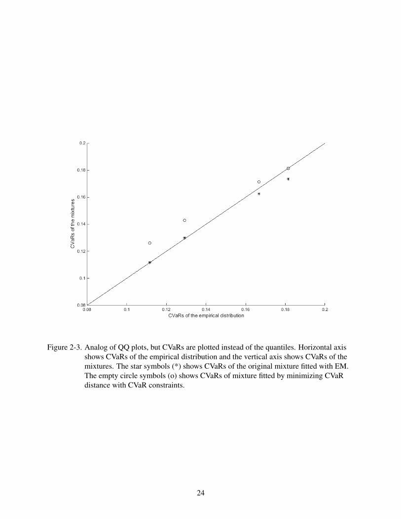
Figure 2-3. Analog of QQ plots, but CVaRs are plotted instead of the quantiles. Horizontal axisshows CVaRs of the empirical distribution and the vertical axis shows CVaRs of themixtures. The star symbols (*) shows CVaRs of the original mixture fitted with EM.The empty circle symbols (o) shows CVaRs of mixture fitted by minimizing CVaRdistance with CVaR constraints.

24

CHAPTER 3OPTIMAL ALLOCATION OF RETIREMENT PORTFOLIOS

3.1 Motivation

The problem of selecting optimal portfolios for retirement has unique features that are not

addressed by more commonly used portfolio selection models used in trading. One distinct

feature of a retirement portfolio is that it should incorporate the life span of an investor. The

planning horizon depends on the age of investor, or more specifically, on a conditional life

expectancy. Another important feature is to guarantee, in some sense, that the individual will be

able to withdraw some amount of money every year from a portfolio by selling some predefined

amount of assets without injecting external funds. Finally, one of the questions that the models

tries to answer is, in what situation is it beneficial to invest in annuity instead of more risky assets.

Most of portfolio optimization literature considers portfolios focusing on risk minimization

with some budget and expected profit constraints. The famous mean-variance (or Markowitz)

portfolio [18] minimizes portfolio variance with constraints on the expected return. There are

many directions that extend the original mean-variance portfolio and deal with its shortcomings.

One direction is to substitute variance with some other risk measures. Variance does not

distinguish positive and negative portfolio returns, however investors are mostly concerned only

with negative returns. [11, 10] and [19] used Conditional Value-at Risk (CVaR) instead of the

variance. CVaR is a convex function of its random variable and therefore problems involving

CVaR can be solved efficiently in many cases. Another important risk measure, which is

frequently used in trading, is drawdown. Drawdown can be optimized with convex and linear

programming, see [20], [21] and [22]. Other extension of the portfolio theory focuses on dynamic

models. In dynamic models the decision to invest is made over time. The dynamic models can be

of two types, continuous-time and discrete-time (multistage) models. In continuous time, the

decision to invest is made continuously and in discrete-time, the investment decisions take place

on specific time moments. For the continuous-time portfolio selection see [23, 24]. For

discrete-time stochastic control model see [25]. A comprehensive literature review on dynamic

models is given in [26]. Multistage models can be formulated as stochastic optimization

25

problems. [27] and [28] developed a general multistage approach for modeling financial planning

problems. [29] and [30] use stochastic programming to solve dynamic cash flow matching and

asset/liability management problems, respectively. In general, it is very hard to solve multistage

stochastic optimization problems formulated with scenario trees, due to the size of the problem

(number of variables) growing beyond tractable bounds. It should be mentioned that calibration

of such trees is a difficult non-convex optimization problem.

In order to avoid the dimensionality problems, [31] models the investment decisions as

linear functions that remain same across all scenarios and produce the investment decision based

on previous performance of the asset.

Takano and Gotoh in [32] model the investment decisions with kernel method, resulting in

the nonlinear control functions depending upon returns of instruments.

We follow ideas of [32] and model multistage portfolio decision process using the kernel

method. The investment horizon is 35 years, starting from the retirement of the investor at the age

of 65. The objective is to maximize the discounted expected terminal wealth subject to constraints

on cash outflows from the portfolio. We generate multiple sample paths of assets prices,

simulated using historical data. for every sample path, the discounted weighted portfolio value is

calculated, where the probabilities of death are used as weights. The probability of death is

calculated from the U.S. mortality tables. The investor wants to have predetermined cash outflows

obtained by selling a portion of the portfolio. Risk of shortage of this cash outflows is managed

by penalizing the cash outflow shortage in the objective function. Furthermore, the monotonicity

constraints are imposed on the cash outflows from the portfolio. Without the monotonicity

constraint the model might not provide the necessary cash outflow on certain periods and instead,

reinvest that amount to increase the expected estate value.

We conducted a case study corresponding to a typical investment decision upon retirement,

in order to reveal the conditions leading to investments in annuities. Two types of asset return

sample paths are considered. First type assumes that the asset returns will be similar to the

historically observed rates of the asset. The second type of sample paths assumes the future asset

26

returns will be significantly lower. These sample paths are created by subtracting 12% from the

historical returns of all assets. The case study shows that for the first type of sample paths, where

rates are similar to the ones observed in the past, investment in the annuities is not optimal.

However, in the case when the asset growth rates are significantly lower, the model invests only in

the annuities.

3.2 Notations

We start with introduction of notations

• N := number of assets available for investments,

• S := number of sample paths,

• T := portfolio investment horizon,

• rsi,t := rate of return of asset i = 1, . . . ,N during period t = 1, . . . ,T in sample path

s = 1, . . . ,S; we will call rate of return by just return and denote the vector of returns by

rst = (rs

1,t , . . . ,rsN,t) ,

• vsm,t = rs

m, . . . ,rst−1 := set of returns observed from period m, until the end of period

t−1 (not including the returns rst ) for sample path s,

• dst := discount factor at time t for sample path s; discounting is done using inflation rate

ρst , ds

t = 1/(1+ρst )

t ,

• pt := probability that a person will die at the age 65+ t (conditional that he is alive at the

age of 65),

• yi := vector of control variables for investment adjustment function,

• f (vst ,yi) := investment adjustment function defining how much investment is made in

each sample path s in asset i at the end of period t,

• G(yi) := regularization function of control parameters,

• K(vsm,t ,v

km,t) := kernel function, k = 1, . . . ,S,

• xsi,t := investment amount to i-th asset at the end of time period t for sample path s,

• xi := investments to i-th asset at time t = 0,

27

• usi,t := adjustment (change in position) of asset i at the beginning of period t for sample

path s,

• Rsi,t := cash outflow resulting from selling an asset i at the end of time t for sample path s,

• V0 := portfolio value at time t = 0 (initial investment),

• V st := portfolio value at time t for sample path s,

• z := investment in annuity at time t = 0(in dollars),

• Ast := yield of annuity at the end of time period t for sample path s,

• L := amount of money that the investor is planing to withdraw as each time t,

• λ := regularization coefficient, λ > 0,

• κt := penalty for the cash flow shortage at time t,

• α := upper bound on sum of absolute adjustments each year, expressed as a fraction of

the portfolio.

3.3 Model Formulation

This section develops a model for optimization of a retirement portfolio. We consider a

portfolio including stock indices, bond indices, and an annuity. The annuity pays amount Ast z at

the end of each period t and does not contribute funds to the expected estate value. Annuity is

bought at time t = 0 and can not be bought or sold after that moment. It is also assumed that the

tax rate is zero (tax free environment).

Given initial investments in assets xi, the dynamics of investments in stocks and bonds are

as follows

xsi,1 = (1+ rs

i,1)xi, (3-1)

xsi,t = (1+ rs

i,t)(xsi,t−1 +us

i,t−1−Rsi,t−1) t = 2, . . . ,T.

Variables usi,t and Rs

i,t control how much is invested at the end of each period in each asset. usi,t is a

position adjustments for asset i at the end of time t for sample path s. Rsi,t is cash outflow from the

28

portfolio, generated from selling asset i at time t for sample path s. The variable usi,t is defined as

usi,t = f (vs

t ,yi), (3-2)

where vst is a set of returns for all assets, up to time t, for sample path s, and yi are some

parameters defining the function f . Therefore, usi,t , are some nonlinear functions of previous

returns of assets. The explicit form of function f is not specified in this section. The only

requirement on function f is that it should be linear in yi, i.e.

f (vst ,γ1y1

i + γ2 y2i ) = γ1 f (vs

t ,y1i )+ γ2 f (vs

t ,y2i ),

where γ1,γ2 ∈ R. Also, it should be noted that the function f does not change with t, however it

takes input vst that depends both on t and s, therefore the position adjustments depend on t and s.

The linearity of f with respect to yi is introduced to formulate the portfolio optimization problem

as a convex programming problem.

The total asset adjustments must sum to 0, this is expressed as a constraint,

N

∑i=1

usi,t = 0 . (3-3)

In addition to (3-3) the sum of absolute adjustments (over each asset i) in each period t and

sample path s is constrained to be less than or equal to some fraction α of the portfolio value in

the previous year of the same sample path,

N

∑i=1|us

i,t | ≤ αV st−1. (3-4)

Constraint (3-4) serves as additional regularization on the adjustments. Without constraint (3-4)

the values of usi,t can potentially be very large in absolute value but cancel out due to opposite

signs and still satisfy (3-3).

The value of the portfolio at the end of time period t for sample path s equals,

V st =

N

∑i=1

xsi,t . (3-5)

29

The objective is to maximize expected estate value of the portfolio. The expected estate value is

the weighted average of the discounted expected portfolio values for each sample path, where the

probabilities of death pt are used as weights. For every sample path s the portfolio value V st , at the

end of time period t, is discounted to time 0 using discounting coefficients dst , defined by

inflation, therefore,

discounted estate value for sample path s =T

∑t=1

ptdst V

st . (3-6)

By averaging over sample paths we obtain the expected estate value,

1S

S

∑s=1

T

∑t=1

ptdst V

st . (3-7)

In order to avoid over-fitting the data, we included the regularization term G(yi), defined for every

instrument i. The total regularization term is

N

∑i=1

G(yi) . (3-8)

The total cash outflow from selling the assets in the portfolio equals

cash flow from portfolio =N

∑i=1

Rsi,t .

The amount of money that the investor receives from the portfolio and annuity at the end of time

period t for sample path s equals Ast z+∑

Ni=1 Rs

i,t . If Ast z+∑

Ni=1 Rs

i,t < L then there is a shortage of

cash outflow and the resulting amount is penalized in the objective. Let κtTt=1 be some

decreasing sequence of positive numbers, the following function is a penalty term of cash outflow

shortages in the objectiveT

∑t=1

κt

[L−As

t z−N

∑i=1

Rsi,t

]+, (3-9)

where [∗]+ = max∗,0. To illustrate why it is important that κtTt=1 is a decreasing sequence,

consider the case where all κt are equal. Also, lets assume that there is a shortage of cash outflow,

equal to the amount w, at some year t > 0. Because, κt are all equal in (3-9), it does not make a

difference for that penalty term if there is a shortage equal to w/t during every year until t, or just

30

a single shortage of w at time t. However, if the amount of w/t is reinvested before time t in the

portfolio, it will(probably) increase in value by the time t and therefore, it will increase the

expected estate value of the portfolio. So, if κtTt=1 is not a decreasing sequence, the model will

try to incur penalty as soon as possible, even if there are enough funds in the portfolio at that

earlier date, and reinvest that shortage amount in the portfolio. Therefore the penalty from

parameters κt should outweigh any possible benefits from reinvesting at earlier dates. A simple

formula for κt is κt = κ(1+ r)T−t , where κ > 1 is some constant and r is some percentage that it

is significantly greater than the average growth rate of any asset considered in the portfolio.

Alternative to (3-9), it is possible to formulate the cash outflow requirement as a constraint

for each time t and sample path s

Ast z+

N

∑i=1

Rsi,t ≥ L. (3-10)

However constraint (3-10) may be violated on some sample paths, where the sampled rates of

returns for assets are particularly low and portfolio value shrinks to 0. Therefore, a better way of

imposing cash outflow requirements as a constraint would be to impose it as CVaR constraint. Let

X be some random variable. Imposing the CVaR constraint assures that the cash outflow

requirement (3-10) will be satisfied most of the time (around 100(1−α/2) percent of the cash

outflow payments will be fully paid). The CVaRα cash outflow requirement is

minζt

(ζt +

1S(1−αt)

S

∑s=1

[−

N

∑i=1

Rsi,t−As

t z−ζt

]+)≤−lt . (3-11)

The CVaRα(X) constraint is less likely to become infeasible since it allows cash outflows to be

less than required amount, on a small percentage sample paths. However, if the confidence

interval is very large and the cash outflow requirements are very high compared to the initial

investment, the CVaRα(X) constraints will become infeasible.

The model includes constraints on monotonicity of the cash outflows from the portfolio

N

∑i=1

Rsi,t−1 ≥

N

∑i=1

Rsi,t . (3-12)

31

Without the monotonicity constraints, the model might not provide necessary cash outflows at the

end of certain years and instead, reinvest that amount to increase the expected estate value of the

portfolio. The monotonicty constraint ensures that the cash outflow shortage occurs only in years

where the portfolio value drops below the cash outflow amount at the end of the previous year.

We minimize the objective function, containing expected costs with minus sign,

regularization term with penalty coefficient λ > 0 and cash outflow shortage with penalty κt

−1S

S

∑s=1

T

∑t=1

ptdst V

st +λ

N

∑i=1

G(yi)+T

∑t=1

κt

[L−As

t z−N

∑i=1

Rsi,t

]+. (3-13)

The explicit form of function G is not defined in this section, however, it is assumed that the

function G(y) is a convex function in y. This is important to formulate the problem as a convex

optimization. The resulting objective function (3-13) is a convex function in yi and linear in V st .

Further we provide the general model formulation.

minus

i,t ,Rsi,t ,

V0,V st ,yi,

xsi ,x

si,t ,z

− 1S

S

∑s=1

T

∑t=1

ptdst V

st +λ

N

∑i=1

G(yi)+T

∑t=1

κt

[L−As

t z−N

∑i=1

Rsi,t

]+(3-14)

s.t.

xsi,1 = (1+ rs

i,1)xi i = 1, . . . ,N; s = 1, . . . ,S

xsi,t = (1+ rs

i,t)(xsi,t−1 +us

i,t−1−Rsi,t−1) i = 1, . . . ,N; t = 2, . . . ,T ; s = 1, . . . ,S

N

∑i=1

xi =V0− z

V st =

N

∑i=1

xsi,t t = 1, . . . ,T ; s = 1, . . . ,S

N

∑i=1

usi,t = 0 t = 1, . . . ,T ; s = 1, . . . ,S

32

N

∑i=1

Rsi,t ≤

N

∑i=1

Rsi,t−1 t = 2, . . . ,T ; s = 1, . . . ,S

usi,t = f (vs

m,t ,yi) i = 1, . . . ,N; t = 1, . . . ,T ; s = 1, . . . ,S

N

∑i=1|us

i,t | ≤ αV st−1 t = 2, . . . ,T ; s = 1, . . . ,S

N

∑i=1|us

i,1| ≤ α(V0− z)

z≥ 0

Rsi,t ≥ 0

xi ≥ 0 i = 1, . . . ,N

xsi,t ≥ 0 i = 1, . . . ,N; t = 1, . . . ,T ; s = 1, . . . ,S

3.4 Special Case of General Formulation

This section presents a special case of the general problem formulation. We picked

functions G(yi) and f (rst ,yi) similar to the model developed in [32].

Let m > 0 be some integer and Km(vst ,v

kt ) be the kernel function defined as follows

K(vsm,t ,v

km,t) = exp

(− σ

m

N

∑i=1

t−1

∑l=t−m−1

(rki,l− rs

i,l)2), (3-15)

where σ > 0 is some constant. The parameter m controls how many previous years of information

is used by the kernel function to calculate the portfolio adjustments. Given (3-15), the control

function f (vst ,yi) is defined as

f (vst ,yi) =

S

∑j=1

y ji K(vs

m,t ,vjm,t), where yi = (y1

i , . . . ,ySi ). (3-16)

Function (3-16) is linear in yi. By substituting (3-16) in constraint (3-2), we get the following

adjustment functions

usi,t =

S

∑j=1

y ji K(vs

m,t ,vjm,t) i = 1, . . . ,N; t = 1, . . . ,T ; s = 1, . . . ,S. (3-17)

33

We use L2 norm as the regularization function G(yi),

G(yi) = ||yi||22 =S

∑s=1

(ysi )

2. (3-18)

Substituting (3-18) in the objective, gives

−1S

T

∑t=1

S

∑s=1

ptdst V

st +λ

N

∑i=1||yi||22 +

T

∑t=1

κt

[L−As

t z−N

∑i=1

Rsi,t

]+. (3-19)

This model can be reduced to convex quadratic problem by linearizing (3-9). Other

formulations are also possible. For example using L1 norm instead of L2 norm in (3-18) leads to

a linear programming formulation after linearization of (3-9). Another variation of this model

could be linear (with respect to rates rsi,t) adjustment functions instead of the nonlinear kernel

adjustment functions. Linear investment adjustments will lead to a lower expected estate value.

However the dimensionality of the problem will be reduced significantly, because the problem

size (the number of parameters to be optimized) will increase linearly with the number of sample

paths, instead of quadratically, with kernel functions.

3.5 Simulation of Return Sample Paths and Mortality Probabilities

3.5.1 Historical Simulations

We simulate return sample paths of considered investment instruments for T years in the

future. The simulations are based on end-of-year data of N assets over T years. Let t ∈ 1, . . . , T

be a year index for a historical dataset and ri,t be a historical return of asset i. The returns of the

indices are represented as the N× T matrix,

r1,1 r2,1, . . . , rN,1

r1,2 r2,2, . . . , rN,2

. . . . . . . . . . . .

r1,T r2,T , . . . , rN,T

(3-20)

We generate return sample paths using the historical simulation method. The historical simulation

method samples a random row from the matrix (3-20) and uses this row as a possible future

realization of returns of instruments. Therefore the future simulation of returns is just sampling of

34

the matrix (3-20) with replacement. Each such sample represents a future dynamics of return of

the assets. Note that the simulation method samples entire row from matrix (3-20), therefore the

correlations among assets are maintained in the random sample.

3.5.2 Mortality Probabilities

Let τ be a random variable that denotes an age of death of the investor. The probability that

an investor dies in time interval [t−1, t) since retirement at the age 65 is defined as follows

pt = P(t +64 < τ ≤ t +65 | τ > 65), t = 1, . . . ,T.

It is possible to calculate pt using the mortality table of USA. Mortality tables give a

conditional probability of death at some age, given that person is alive at year earlier of that age.

We use the mortality Table 3-1, which gives probability pt that t +64 < τ ≤ t +65, conditional

that τ > t +64,

pt = P(t +64 < τ ≤ t +65|τ > t +64), t = 1, . . . ,T.

It can be shown that

60 70 80 90 100 110 120

Age

0

0.01

0.02

0.03

0.04

0.05

Pro

babili

ty

Male

Female

Figure 3-1. Mortality probability graph. Probabilities that person dies while he/she is t +64 yearsold (t = 1, . . . ,T ), conditional that he/she is alive at the age of 65.

35

Table 3-1. USA Mortality table for the year 2016 with probabilities of death for male and femaleUSA citizens. This table can be found at US Social Security website:https://www.ssa.gov/oact/STATS/table4c6.html

Age p(age) Male p(age) Female65 0.0158 0.009866 0.0170 0.0107. . . . . . . . .119 0.8820 0.8820

pt =

pt , if t = 1

pt ∏t−1j=1(1− p j), if t = 2, . . . ,T

Figure 3-1 shows pt as the function of age t .

3.6 Case Study

3.6.1 Case Study Parameters

This case study considers a typical retirement situation in USA. Two variants of future asset

return sample paths are considered. These two variants correspond to an optimistic and

pessimistic projections regarding the future market dynamics. In the optimistic case, the future

returns over 35 years, for all instruments, are sampled from the historical returns over the recent

30 years. In the pessimistic case, the market is assumed to enter into a stagnation, similar to the

Japaneses market, which has approximately zero cumulative return for the recent 30 years. In the

pessimistic case, 12% is subtracted from each asset return, every year for every sample path.

Here are parameters of the model, which correspond to the retirement conditions in USA.

• The retiree is 65 years old.

• Investment horizon is 35 years.

• Portfolio is re-balanced at the end of each year.

• Retiree is a male (mortality probabilities for males are used in objective function).

• $500,000 is available for investment at time t = 0.

• Yearly inflation rate is 3% during the entire investment horizon.

• Yearly rate of return of annuity is 5%.

36

• Adjustment rules use kernel functions with parameter σ = 1.

• λ = 100

• κt = 2 ·1.2(35−t)

• α = 20%

• m = 5

There are 10 stock and bond indexes available for investment, see Table 3-2.

Table 3-2. The list of assets in the retirement portfolio.Index Name Index AbbreviationBarclays Muni FI-MUNIBarclays Agg FI-INVGRDRussell 2000 USEQ-SMRussell 2000 Value USEQ-SMVALRussell 2000 Growth USEQ-SMGRTHS&P 500 USEQ-LGS&P 400 Mid Cap USEQ-MIDS&P Citi 500 Value USEQ-LGVALS&P Citi 500 Growth USEQ-LGGRTHMSCI EAFE NUSEQ

For each index, 30 years of yearly returns (from 1985, to 2015) are used to create future

return sample paths. Each sample path includes 35 yearly returns, sampled from the 30 year

historical dataset (see the Historical Simulation method in Section 3.5). 200 sample paths are

generated for both, optimistic and pessimistic cases. 100 sample paths out of 200, for both

optimistic and pessimistic datasets, are used to find optimal investment rules in the model.

Therefore, the model is fitted on 3500 data points (asset returns) sampled from historical

observations. The remaining 100 sample paths, not included in the optimization, are used for

evaluating the out-of-sample performance of the model.

3.6.2 Optimal Portfolio

The considered optimization problems are reduces to Quadratic Programming, by

linearizing function (3-9) in the objective. Gurobi version 8.1.0 and Pyomo version 5.5.0 are used

for solving th resulting quadratic programming problem. The following case study link contains

37

the corresponding code:

http://uryasev.ams.stonybrook.edu/index.php/research/testproblems/financial engin

eering/case-study-retirement-portfolio-selection/.

The coefficients of the adjustment functions yi, are obtained by solving the quadratic

optimization problem corresponding to the optimal portfolio problem (3-14). Next, the

adjustment values for the out-of-sample dataset are evaluated, according to the formula (3-16).

The adjustment functions, for end of the time moment t, take previous m rates of returns of all

assets in the portfolio, observed in time interval [t−m, t−1] and produce an asset adjustment for

that time moment. Note that returns that go into these functions are different for each sample

path, therefore the adjustment values will be different for each sample path as well.

In order to calculate the portfolio values on the out-of-sample data, the cash outflows Rsi,t

are required. The model does not provide the cash outflow Rsi,t for the out-of-sample paths, as

those values are calculated for the in-sample paths. Therefore, it is unclear what values of Rsi,t

should be use in the out-of-sample paths. Additionally, despite the constraint on positivity of asset

positions in the in-sample optimization problems, a small portion of the assets may be allocated to

short positions in out-of-sample runs. Usually, the retirement portfolios do not have short

positions, since it is considered a risky strategy and therefore not suitable for a risk averse retiree

investors. Next, we show how to circumvent these problems for the out of sample datasets.

Let Ps,t+ and Ps,t

− be the total dollar investment in long and short positions, in a portfolio at

the end of time period t for sample path s,

Ps,t+ =

N

∑i=1

[xsi,t ]

+ ,

Ps,t− =

N

∑i=1

[−xsi,t ]

+.

The cash outflows are calculated as follows

Rsi,t =

L[xs

i,t−1]+

Ps,t−1+

if Ps,t−1+ > L

xsi,t−1 otherwise

(3-21)

38

So the cash outflows originate only from the long positions and are proportional to Ps,t−1+ .

All short positions, at the end of time period t for sample path s, are set to 0. As a result, the

amount of money equal to Ps,t− has to be subtracted from the remaining (long) part of the portfolio.

To shrink the portfolio by Ps,t− , each long asset position is reduced in a proportion to Ps,t

+ . Thus,

the new positions xsi,t are

xsi,t =

0, if xs

i,t ≤ 0

xsi,t−

xsi,t

Ps,t+

Ps,t− , otherwise.

Tables 3-3 through 3-7 show the average (over sample paths) investments in assets over

time for optimistic out-of-sample paths, corresponding to the model (3-14), with the minimum

cash flows requirements L ∈ $10,000;$30,000; . . . ,$90,000. Tables 3-8,3-9 and 3-10 show the

average (over sample paths) investments in assets over time for pessimistic out-of-sample paths,

corresponding to the model (3-14), with the minimum cash flows requirements

L ∈ $10,000;$25,000;$30,000;$50,000. Tables 3-8,3-9 and 3-10, show that, in the

pessimistic case, for L = $10,000, the model invests 30% of funds in the annuity and for

L = $25,000, 100% of investment goes into the annuities. However for L = $30,000 the model

decreases the annuity investment to 56%. As for L = $50,000 (and higher) nothing is invested in

the annuities and the model selects the stock/bond indexes. The Figure 3-2 shows the average

(taken over sample paths) portfolio values through time, constructed using the adjustment

functions, corresponding to the model (3-14) with the minimum cash flows requirements of

L ∈ $10,000;$30,000; . . . ,$90,000. However in the optimistic sample paths, the model does

not invest in annuities at any minimum cash outflow requirement L.

39

Table 3-3. Average investment in assets, L = $ 10,000, optimistic out-of-sample paths (inthousand dollars). Average is taken over sample paths.

Asset Investment t=0 t=5 t=10 t=15 t=20 t=25 t=30 t=35Annuity 0 0 0 0 0 0 0 0FI-MUNI 0 0 0 0 0 0 0 0FI-INVGRD 0 3 4 6 7 11 16 25USEQ-SM 0 0 0 0 0 0 0 0USEQ-SMVAL 0 28 54 104 171 360 635 1,177USEQ-SMGRTH 0 1 1 2 4 7 13 19USEQ-LG 0 0 0 0 0 0 0 0USEQ-MID 500 779 1,475 2,791 4,993 10,593 20,183 36,797USEQ-LGVAL 0 0 0 0 0 0 0 0USEQ-LGGRTH 0 4 8 15 30 72 139 380NUSEQ 0 50 80 153 268 444 762 1,186


Asset Investment t=0 t=5 t=10 t=15 t=20 t=25 t=30 t=35Annuity 0 0 0 0 0 0 0 0FI-MUNI 0 0 0 0 0 0 0 0FI-INVGRD 3 34 44 51 64 95 138 194USEQ-SM 0 0 0 0 0 0 0 0USEQ-SMVAL 69 28 57 105 192 366 592 1,121USEQ-SMGRTH 0 1 2 4 7 14 27 42USEQ-LG 0 0 0 0 0 0 0 0USEQ-MID 402 612 1,025 1,818 3,136 6,642 12,574 22,657USEQ-LGVAL 0 0 0 0 0 0 0 0USEQ-LGGRTH 25 30 54 102 181 448 920 2,594NUSEQ 0 45 69 124 209 365 628 996

40


Asset Investment t=0 t=5 t=10 t=15 t=20 t=25 t=30 t=35Annuity 0 0 0 0 0 0 0 0FI-MUNI 0 7 7 7 7 10 14 21FI-INVGRD 330 244 202 206 246 328 492 680USEQ-SM 0 0 0 0 0 0 0 0USEQ-SMVAL 57 137 194 281 424 693 1,163 1,875USEQ-SMGRTH 0 0 0 0 0 0 0 0USEQ-LG 0 0 0 0 0 0 0 0USEQ-MID 36 47 58 84 108 224 416 820USEQ-LGVAL 0 0 0 0 0 0 0 0USEQ-LGGRTH 77 65 66 92 157 386 857 2,515NUSEQ 0 33 35 74 104 154 255 349


Asset Investment t=0 t=5 t=10 t=15 t=20 t=25 t=30 t=35Annuity 0 0 0 0 0 0 0 0FI-MUNI 0 0 0 0 0 0 0 0FI-INVGRD 195 117 67 40 32 35 44 56USEQ-SM 0 0 0 0 0 0 0 0USEQ-SMVAL 46 66 67 48 43 65 99 132USEQ-SMGRTH 0 0 0 0 0 0 0 0USEQ-LG 0 0 0 0 0 0 0 0USEQ-MID 107 118 73 69 88 170 320 596USEQ-LGVAL 0 0 0 0 0 0 0 0USEQ-LGGRTH 136 92 77 90 142 350 748 2,300NUSEQ 16 67 48 35 42 78 162 300


Asset Investment t=0 t=5 t=10 t=15 t=20 t=25 t=30 t=35Annuity 0 0 0 0 0 0 0 0FI-MUNI 0 0 0 0 0 0 0 0FI-INVGRD 65 54 17 6 5 5 6 7USEQ-SM 0 0 0 0 0 0 0 0USEQ-SMVAL 70 83 51 30 29 46 76 115USEQ-SMGRTH 0 0 0 0 0 0 0 0USEQ-LG 0 0 0 0 0 0 0 0USEQ-MID 164 85 30 28 33 67 133 302USEQ-LGVAL 0 0 0 0 0 0 0 0USEQ-LGGRTH 140 107 56 48 76 204 439 1,522NUSEQ 61 58 26 12 9 14 23 42

41

Table 3-8. Average investment in assets, L = $ 10,000, pessimistic out-of-sample paths (inthousand dollar). Average is taken over sample paths.

Asset Investment t=0 t=5 t=10 t=15 t=20 t=25 t=30 t=35Annuity 147 147 147 147 147 147 147 147FI-MUNI 0 0 0 0 0 0 0 0FI-INVGRD 1 3 3 2 2 2 1 1USEQ-SM 0 0 0 0 0 0 0 0USEQ-SMVAL 2 3 2 3 2 1 1 0USEQ-SMGRTH 0 0 0 1 0 0 0 0USEQ-LG 0 0 0 0 0 0 0 0USEQ-MID 350 350 360 378 384 355 311 303USEQ-LGVAL 0 0 0 0 0 0 0 0USEQ-LGGRTH 0 4 7 7 7 5 5 4NUSEQ 0 4 4 3 3 3 2 2



42





43

0 5 10 15 20 25 30 35Years

0

5

10

15

20

25

30

35

40

Averag

e Po

rtfolio Value

(in million

s of d

ollars) L = 10K

L = 30KL = 50KL = 70KL = 90K

Figure 3-2. Portfolio values for optimistic out-of-sample paths. The average(over sample paths)portfolio value for the optimistic out-of-sample dataset, constructed using adjustmentfunctions, corresponding to model (3-14) with minimum cash outflow requirementsL ∈ $10,000;$30,000; . . . ,$90,000

44

3.6.3 Expected Shortage Time for Different Cash Outflows

When the investor demands higher cash outflows from the portfolio, the expected estate

value of the portfolio will decrease. Further, with higher cash outflow demands, there are higher

chances that there will not be enough money in the portfolio, at some point, to finance any

outflows.

To measure the cash outflow shortage resulting from the different values of L, the following

measure, named Expected Shortage Time (or ETS) is defined

ET S(L) =1S

S

∑s=1

T

∑t=1

pt(T − t)

(L−∑

Tt=1 Rs

i,t

)+L

ETS is measured in years and calculates the amount of time the retiree will spend without the

necessary cash outflow L, i.e. the number of years he/she will expect to be on Social Security.

The parameters of the case study are used to construct the ETS values for the optimistic and

pessimistic cases. ETS is calculated on the in-sample data, for the cash outflow values of

L ∈ $10,000;$15,000; . . . ;$100,000. The resulting ETS values are shown on Figures 3-3 and

3-4 for optimistic and pessimistic sample paths respectively.

The Figure 3-3 shows that, in the optimistic sample paths, the retiree can have cash outflows

up to $50,000, without expecting any shortages given an average life span. For the values of L

greater than $50,000, the ETS grows roughly linearly. For L = $100,000 the retiree will spend

most of his expected life without necessary cash outflow, because the portfolio can not provide

this much cash outflow, given the initial investment of $500,000.

It should be noted that, in the pessimistic case, if L≤ $25,000 the annuities can fully cover

the cash flow requirements and therefore ETS = 0. However, if L > $25,000 the investment in the

annuities can no longer cover the cash outflow requirements. Even if the entire initial investment

goes into the annuities, it will provide only A · z = 5% ·$500,000 = $25,000. Therefore, for L

values higher than $25,000, the model starts to invest in stock and bond indexes and the ETS is

greater than 0.

45

For the pessimistic sample paths, if the cash flow requirement is L = $100,000 the ETS is

almost equal to the life expectancy of the retiree. This happens because, on most pessimistic

sample paths, the portfolio shrinks to 0 in a 3 or 4 years for L = $100,000. However, if

L = $30,000, on the pessimistic sample paths, the retiree still has relatively small ETS values of

around 3 year.

Higher values of expected estate result in lower values of ETS. Figure 3-5 illustrates the

relationship between expected estate and ETS relationship for the case of optimistic sample paths.

Figure 3-5 is constructed by solving problem (3-14) for cash outflow values of

L ∈ $10,000;$15,000; . . . ;$100,000 and plotting the resulting values of ETS and expected

estate.

20 40 60 80 100Required Cash Flow (in thousands of dollars)

0

1

2

3

4

5

6

7

8

Years

Figure 3-3. ETS values for the optimistic sample paths. Required cash flowsL ∈ $20,000;$30,000; . . . ;$100,000

46

20 40 60 80 100Required Cash Flow (in thousands of dollars)

0

2

4

6

8

10

12Ye

ars

Figure 3-4. ETS values for the pessimistic sample paths. Required cash flowsL ∈ $10,000;$15,000; . . . ;$100,000

Another way to illustrates these relationships is a trade-off between the expected estate (3-7)

and the ETS. Figure 3-5 illustrates the relationship between expected estate and ETS for the set of

optimistic sample paths. Figure 3-5 is constructed by solving problem (3-14) for cash outflow

values of L = $10,000;$15,000; . . . ;$100,000 and plotting the resulting values of ETS and

expected estate. Each marker dot on the curve is a different level of target cash flow (lowest on

the left). When the cash outflow requirements are low, then the expected estate is high – around

$2 million with a $20,000 target - and the expected number of years without cash flow is very low

– or zero. Of course, existence will be close to Social Security standards, but the heirs will be

happy. As the cash outflow requirement rises to around $50,000 to $60,000 per year, the expected

estate drops below $500,000 and one can expect to spend almost a year on social security. At

higher target levels the expected estate drops even further and the time on Social Security rises.

To be clear, these are expected levels. In any specific sample path, once the portfolio goes to zero

no further cash is available for distribution, however long one lives. On the other hand, in very

fortuitous sample paths, portfolio values may not dip to zero for a very long time.

47

0 1 2 3 4 5 6 7 8ETS

0.0

0.5

1.0

1.5

2.0

2.5

3.0

3.5Ex

pected

Estate Va

lue

Figure 3-5. Relationship between expected estate value and the ETS, for the optimistic samplepaths.

48

CHAPTER 4A NEW APPROACH TO CREDIT RATINGS

4.1 Motivation

At the height of the financial crisis of 2008, American International Group, Inc. (AIG), once

the largest insurance company in the US, was rescued from bankruptcy by a US government

bailout worth $85 bn [see, e.g., 33]. This was part of the Troubled Asset Relief Program (TARP)

that cost the US taxpayer in excess of $245 bn. What caused the companies that enjoyed stable

AAA credit ratings to fail abruptly and what role did credit ratings play in the failure?

Early post-crisis literature focused on issues of risk mispricing caused by using dependence

models that fail to accommodate realistic tail behavior of joint defaults and on issues around

structured finance where loan securitization obscured the true riskiness of the collateral. For

example, [34] and [35] provide two different perspectives at how securitized risky debt was

repackaged as virtually risk-free. What is common in the two papers is that they show how rating

agencies were simply unfamiliar with assessing creditworthiness of financial instruments that

cannot be ascribed to a single company and instead involve a pool of loans, bonds and mortgages

from various sources. Thus, the subsequent issues of claims – known as synthetic instruments –

against those assets, were not supported by a robust methodology for pricing their riskiness.

[34] make the point that the new developments in structured finance amplified errors in risk

assessment, while [35] shows that the commonly used dependence assumption known as the

Gaussian copula was inappropriate. As a result, relatively minor imprecisions in credit risk

estimation could have led to variations in default risk of the synthetic securities that were large

enough to cause an AAA-rated security to default with a high probability.

Moreover, [36] looked at a large number of mortgage-backed securities (MBS), collaterized

debt obligations (CDO) and other structured finance securities and found empirical evidence that

higher credit ratings were closely associated with higher MBS prices after controlling for a large

set of security fundamentals. They report that, in terms of value, 80 to 90 percent of sub-prime

MBS initially received AAA ratings but were in effect 6-10 rating notches lower1. This offers

1Rating agencies commonly use 21-22 notch scales, from AAA to C or AAA to D.

49

support for the widely held belief that more conservative credit ratings would have muted the

crisis by making credit more expensive and providing a more reliable information about synthetic

instruments to less informed investor. [37] describe the various conflicts of interest that may have

added to the inability or unwillingness of credit rating agencies to do that.

Moody’s, Standard and Poor’s and Fitch Group – the three major credit rating agencies

known as the Big Three – have evolved since then. They are now more mindful of joint tail risk

and synthetic instruments are hardly new any more. More recent papers on this topic focus on

how credit rating inflation is affected by competition between agencies, by regulation of the

industry and by the business cycle [see, e.g., 38, 39, 40, 41, 42, 43, 44, 45]. For example, [38] find

evidence that credit ratings are inflated during the boom periods and [45] present a model where

ratings quality is counter-cyclical. It is noteworthy that the “boom bias” in these papers does not

result from changes in legislation or competitive pressures surrounding rating agencies. Rather it

comes from the rating agencies’ incentive conflicts.

Credit ratings continue to form the basis of credit assessment. They serve as inputs into

numerous risk assessment tools such as CreditMetrics of JP Morgan, and they are widely used to

determine optimal debt ratio and other aspects of firm’s investment decisions [see, e.g., 46, 47].

For example, Standard and Poor’s now rates over $10 tr in bonds and other assets in more than 50

countries.

In this paper we argue that the fundamental properties of credit ratings have not been given

sufficient attention. Incentive conflicts aside, the current credit ratings are prone to massive

underestimation of risk. The reason is that they are still primarily guided by the probability of

exceedance (PoE), a risk measure which, in addition to suffering from a number of computational

issues, estimates the chance of a default-level loss, not the loss given default. We argue that

extreme risk exposure can still be concealed behind a high credit rating, which has far reaching

implications for financial modeling and operation.

We offer an alternative, more conservative, approach based on a buffered version of PoE.

This new measure – referred to as Buffered Probability of Exceedance (bPoE) – is tied to a loss

50

threshold, akin to PoE. Unlike PoE, bPoE takes into account the magnitude of tail outcomes

exceeding the threshold. It is possible to stretch the tail of the loss distribution and increase the

exposure without increasing PoE, but not without increasing bPoE.

More formally, bPoE is the probability of a tail event with the mean tail value equal to a

specified threshold. Therefore, by definition, bPoE controls both the average magnitude of the tail

and its probability, adding a “buffer” to PoE. The probability measure bPoE is an inverse function

to the Expected Shortfall (ES) coherent risk measure, which is also called Conditional

Value-at-Risk (CVaR), Superquantile, Average VaR and Tail VaR. In this paper we will use

interchangeably the ES and CVaR terms (the ES term is included in the financial regulations and

the CVaR term is used in risk management and optimization applications, which we are referring

to in this paper). In the engineering literature, the concept of bPoE has been introduced by [48] as

an extension of the buffered failure probability proposed by [49] and explored by [50].

From the computational perspective, bPoE has considerable advantages compared to PoE.

First, bPoE has an analytic representation through a minimization formula [see 48], similar to

CVaR [see 10]. Moreover, bPoE is quasi-convex [see, e.g., 48], similar to CVaR which is convex

[see, e.g., 10]. This means that there are efficient algorithms for solving optimization problems

involving these measures. Second, bPoE is a monotonic function of the underlying random

variable and a strictly decreasing function of the threshold on the interval between the mean value

and the essential supremum. This avoids discontinuity of PoE for discrete distributions.

The link between bPoE and ES is not surprising but has been overlooked. In response to the

2007-2009 crisis, the Basel Committee on Banking Supervision, among other measures, moved

from using an unconditional Value-at-Risk (VaR) to ES in order to provide an additional buffer to

capital reserve requirements of financial institutions. Yet, no equivalent move has been

implemented in the way credit ratings are constructed. Similar to capital reserve requirements, the

difference between bPoE and PoE is most pronounced for extremely heavy tailed distributions of

losses, so PoE-based ratings fail when they are needed most – at times of distress. Regarding

numerical implementation of risk constraints, there is an equivalence between risk constraints on

51

CVaR and bPoE [see 48], similar to the equivalence of risk constraints on VaR and PoE.

Therefore, bPoE risk constraints can be replaced by CVaR constraints, as described by [10].

The paper is organized as follows. Section 2 discusses how credit rating construction is

guided by the probability of exceedance. Section 3 provides additional motivation for using

bPoE. Section 4 studies the disparity between the two measures under the most popular statistical

distributions used in structured finance and discusses how we can estimate bPoE. In Section 5 we

analyze the adjustments to traditional credit ratings needed to reflect the use of the new measure.

Sections 6 and 7 offer several special cases where the distinction bPoE vs PoE matters. In

particular, we show (a) what happens to creditworthiness of an insurance company as it

accumulates exposure in the way AIG did in the early 2000s, (b) how to solve the problem of

optimal CDO structure under credit rating constraints when the use of standard ratings is

suboptimal. Additionally, Section 7 contains some detail of a numerical case study which is

posted online in its entirety, including codes, data and results.

4.2 Credit Ratings and Probability of Exceedance

As a risk measure, bPoE has gained initial popularity in areas where tail events can be

catastrophic. For instance, in engineering it has been used to assess tropical storm damages [see,

e.g., 51] and to optimize network infrastructure [see, e.g., 52]. Now the popularity is extending to

other areas of risk analytics. For example, in machine learning, it has been used to improve on

data mining algorithms [see, e.g., 53, 54]. However, it has not been introduced to finance, except,

perhaps, in asset and liability management [29].

Traditionally, credit ratings are driven by historical default rates. These rates are used to

estimate the likelihood of a financial loss exceeding the default threshold for a given security or

debtor [see, e.g., 55, Ch. 2]. Of course, credit ratings are assigned to different entities in different

ways. For example, for large issuers, agencies initiate the construction of a rating; for others, a

debtor approaches an agency. Rating of some securities and debtors involves a large amount of

non-quantitative information collected by credit analysts; for others, only quantitative information

is used.

52

For example, for assigning a rating grade to a company, credit agency analysts usually

request financial information about it, consisting of several years of audited annual financial

statements, operating and financing plans, management policies, and other credit factors affecting

the risk profile of the entity. Some agencies claim to incorporate the extend of potential loss and

recovery rates into the risk profile, however, the way it is done is not disclosed and, at best, this

information affects ratings indirectly as an element of the risk profile.

All this information goes into constructing a credit score, reflecting the likelihood of

default, obtained using a rating algorithm such as a logit model, discriminant analysis and, more

recently, machine learning classification techniques such as support vector machines and artificial

neural networks. Usually, securities or debtors with a similar risk profile will be assigned to the

same rating grade. Sometimes, expert judgments override a rating assignment produced by the

algorithm.

Based on the credit scores, probabilities of default are assigned. Using the historical data

available to a rating agency and the risk profile of the security or debtor, an agency assigns a

rating if probability of default, that is PoE of a given default threshold, is inside a range of default

probability characterizing that specific rating grade. Agencies publish tables of default

probabilities for each rating grade over a given time horizon. Table 4-1 contains Standard and

Poor’s global corporate average cumulative default rates. The data for Table 4-1 is taken from

2016 Corporate Default S&P Study [56]. For example, the BBB rating is assigned to an entity

with one-year PD in the range 0.08% < PD≤ 0.23%.

As an illustration of how PoE guides the construction of credit ratings, it is useful to think

of a synthetic instrument within a simple [57] model. This is a security for which rating agencies

usually use complicated, but exclusively quantitative, models reflecting the various assumptions

and approaches involved in constructing the instruments.

Suppose that a firm finances its operation by issuing a single zero-coupon bond with face

value BT payable at time T . Assume that at every time t ∈ [0,T ] the company has total assets At .

It is standard in the Merton model to assume that At follows a Geometric Brownian motion and

53

Table 4-1. S&P global corporate average cumulative default rates (1981-2015) (%).Rating \Time 1 2 3 4 5AAA 0 0.03 0.13 0.24 0.35AA 0.02 0.06 0.13 0.23 0.34A 0.06 0.15 0.26 0.4 0.55BBB 0.19 0.53 0.91 1.37 1.84BB 0.73 2.25 4.07 5.86 7.51B 3.77 8.56 12.66 15.82 18.27CCC/C 26.36 35.54 40.83 44.05 46.43Investment grade 0.1 0.28 0.48 0.73 0.98Speculative grade 3.8 7.44 10.6 13.15 15.24All rated 1.49 2.94 4.21 5.27 6.17

that default of the company occurs when the firm has no capital (equity) to pay back the debt

holders. Because the zero-coupon pays only at time T , default can occur only at T .

The probability of default at time T equals P(default) = P(AT < BT ). This formula can be

rewritten in terms of PoE by changing the sign of assets and liabilities,

P(default) = P(AT < BT ) = P(−AT >−BT ).

Thus, PD is a PoE of the random variable −AT exceeding the threshold −BT and the probabilities

in Table 4-1 can be used to convert the PD into a rating and vice versa.

Figure 4-1 illustrates PoE as the shaded area 1−α . If we define Value-at-Risk (VaR) as the

loss that is exceeded no more than a given (small) proportion of time 1−α , then it is clear from

Figure 4-1 that PoE is simply one minus the inverse of VaR. Consequently, PoE-based constraints

are equivalent to VaR-based constraints. Hence they are equivalent in terms of rating-based

constraints employed by firms in capital structure and investment decisions.

4.3 Motivation for bPoE-based ratings

The PoE-VaR pair has been criticized on a number of conceptual and computational

grounds. First, VaR is not a coherent risk measure because it fails the sub-additivity condition,

which implies in essence that a diversified portfolio may have a higher, rather than lower, VaR

[see, e.g., 58, 59]. Second, VaR is discontinuous, non-differential and non-convex for empirical

distributions – a major numerical difficulty for optimization algorithms. In particular, when it is

necessary to minimize PoE or to impose a PoE constraint, the resulting optimization models are

54

0 0.5 1 1.5 2 2.5 3

0

0.2

0.4

0.6

0.8

1

x = lower bound

Figure 4-1. Relationship between PoE and VaR.

often intractable. Most importantly, the PoE-VaR pair does not account for the magnitude of the

loss given default (LGD). Losses of vastly different expected value can have the same VaR and

thus rating-based constraints may obscure massive risk exposure.

The PoE-VaR pair offers an overly optimistic measure of risk due to insensitivity to the tail

properties of the distribution of losses. For two loss distributions, one with a heavier tail than the

other, PoE-based ratings can be identical (in some cases, the instrument with heavier-tailed losses

might have a higher rating). Figure 4-2 illustrates this situation using the normal and log-normal

distributions.

It is not difficult to see that CVaR is related to bPoE in the same way as VaR is related to

PoE: bPoE is simply one minus the inverse of CVaR. Figure 4-3 illustrates this relationship with

bPoE represented by the shaded area. It is clear from Figure 4-3 that bPoE measures the

probability of a tail event with expected loss equal to CVaR, which captures LGD. This

recognizes the shortcomings of the PoE-VaR pair that have led the Basel Committee to adopt

CVaR for capital reserve calculations.

55

0 0.5 1 1.5 2 2.5 3 3.5 4 4.5 5

0

0.1

0.2

0.3

0.4

0.5

0.6

0.7

0.8

given default for

company 1

expected loss

given default for

company 2

expected loss

Figure 4-2. Loss distributions for two companies with equal PoE.

In the setting of credit ratings, the ‘buffer’ interpretation of bPoE is obtained by setting the

threshold CVaR at the value of VaR and recovering the difference between bPoE and PoE. It is no

surprise that bPoE is no less than PoE for any non-degenerate distribution and the difference can

be viewed as a cushion for the LGD implicit in the rating, similar to how CVaR provides a

cushion in capital reserves. Since VaR has been supplemented by CVaR in financial industry, it

follows naturally that PoE needs the same upgrade.

As mentioned in the introduction, credit ratings have direct influence on prices of financial

assets and firm’s capital structure and investment decisions and thus debtors might have

incentives to inflate ratings. Often, credit ratings work on the ‘issuer pays’ basis, where the issuer

of the security pays to get a rating from the Big Three, which implies an incentive conflict.

Debtors may have incentive to exploit weaknesses of existing credit rating models.

Comprehensive risk profiling by a rating agency may be able to spot an excessive LGD and

this will translate into a hopefully higher PoE of a default loss. However, even if rating agencies

are incentivized to do that, the credit scores they produce are based on historical default rates.

56

0 0.5 1 1.5 2 2.5 3

0

0.2

0.4

0.6

0.8

1

x = average

Figure 4-3. Relationship between bPoE and CVaR.

Thus they reflect the likelihood of default, not the buffered likelihood of default. In order words,

by not accounting for LGD explicitly, traditional ratings do not distinguish clearly between

securities and debtors that have a major impact on the investor in case of default, from those that

do not.

In certain cases, credit ratings are assigned using only quantitative information and

securitization conceals LGD. In particular, for the synthetic instruments such as CDOs, it is

possible to clearly define an event of default of its tranches – see Section 7. This event is usually

expressed as the loss exceeding some threshold value, known as an attachment point of the

tranche. Having a clear definition of default of a tranche and well specified distribution of losses

for the asset pool underlying the CDO, we can compute the probability of default. Based on this a

rating grade of a tranche is assigned. However, the joint loss distribution for a large and diverse

pool of assets, e.g., bonds and mortgages, may be unavailable to the agency. In this case, credit

rating of securitized debt may raise both conceptual and computational difficulties.

57

Contrary to PoE, bPoE has exceptional mathematical properties. It is a quasi-convex

function of the loss which makes it a desirable function for optimization models. In particular,

minimization models with bPoE inequality constraints can lead to convex or even linear

programming problems, which can be solved very efficiently, in contrast to discontinuous and

non-convex problems associated with PoE constraints. This offers a potential for efficient

solutions to firm’s investment and capital structure problems with rating-based constraints [see,

e.g., 60, 61].

4.4 bPoE Definition and Estimation

We now turn to the mathematical and statistical properties of the bPoE-CVaR pair and

compare them to the PoE-VaR counterparts. We start by re-emphasizing that non-sub-additivity

makes VaR a non-convex function. Non-convexity means that optimization problems with VaR

constraints or with a VaR objective function are, in general, intractable for large dimensions. At

the same time, optimization problems involving CVaR constraints or with CVaR as the objective

function, are usually solvable in polynomial time, using convex or even linear programming

methods.

Despite the wide adoption of CVaR in financial industry, there has not been an analogous

substitution of the PoE-based methodologies with bPoE-based methodology, even though bPoE

inherits similar desirable mathematical properties from CVaR. For example, it is possible to solve

a large dimensional portfolio optimization problem with a constraint on bPoE of the portfolio loss

at a speed many times faster than the equivalent problem with PoE-based constraints.

We now define the relevant risk measures formally. Let X denote a random loss, FX its

cumulative distribution function and α ∈ [0,1) some confidence level, then VaR (or a quantile of

X) can be defined as

VaRα(X) = inf

v ∈ R | FX(v)≥ α

The relationship between bPoE and PoE is similar to that between CVaR and VaR. The

value of bPoE with threshold v of a random variable X equals to the probability mass in the right

58

tail of the distribution of X such that the average value of X in this tail is equal to the threshold v.

It is convenient to define bPoE formally as follows, by using the minimization representation [see,

e.g., 48]

bPoEv(X) = infa≥0

E[a(X− v)+1]+ . (4-1)

Because bPoE is equal to one minus the inverse function of CVaR, where CVaR gives the average

value in the tail having probability 1−α , bPoE equals to PoE for the right tail with CVaR equal

to v.

The asymptotic results by [62] suggest a simple estimator of bPoE. Let xini=1 denote an

iid sample of realizations of X . Under fairly general conditions, any quantile of the distribution of

X can be consistently estimated by its empirical counterpart. The corresponding CVaR is just the

sample mean over the observations exceeding the relevant empirical quantile. Given these

estimates, it is natural to estimate bPoE by the sample equivalent of the population problem in

(4-1) as follows

bPoEv = mina≥0

1n

n

∑i=1

[a(xi− v)+1]+ Iv < max(x1, . . . ,xn)

,

where Ix is the indicator function and v can take any estimated CVaR value.

The resulting estimator converges to bPoE uniformly in v at the√

n-rate. If quantiles are

unique, then the solution is

a∗ =1

v−qα(X),

where qα(X) is the (1−α)% quantile of X . In this case,

bPoEv =1n

n

∑i=1

[a∗(xi− v)+1]+

and [62] show that√

n(bPoEv−bPoEv(X))→ N(0,σ2v ), for any v,

where σ2v =Var ([a∗(X− v)+1]+).

59

For any consistent estimator a of a∗, a consistent estimator of σ2v can be obtained as follows

σ2v =

1n−1

n

∑i=1

([a(xi− v)+1]+− bPoEv

)2.

This gives grounds to statistical inference about the buffer in terms of economic and statistical

significance.

An important consequence of these asymptotic results is that standard models of dynamic

quantiles of financial returns, including popular GARCH specifications and quantile regressions,

can be effectively used in evaluating bPoE. To rating agencies, they permit credit scoring to be

based on models of buffered likelihood of default and the resulting credit ratings to include an

explicit buffer for LGD.

A suite of standard statistical results also follow from this asymptotic distribution. For

example, the (1−β )100% asymptotic confidence bands for bPoE at a given quantile v can be

written as [qβ

L (v), qβ

U(v)], where

qβ

L (v) = max(

0, bPoEv(X)−Φ−1(

β) σv√

n

)(4-2)

qβ

U(v) = min(

1, bPoEv(X)+Φ−1(

β) σv√

n

)(4-3)

and Φ−1( · ) is the inverse of standard normal cdf. Using formulas (4-2) and (4-3), it is easy to

calculate the sample size needed in order to achieve a given precision in estimating bPoE with a

desired confidence.

4.5 bPoE Ratings

The idea of the proposed methodology is to use bPoE to guide the construction of credit

ratings and the use of rating-based constraints. This means, in order to assign a rating grade, we

propose estimating bPoE for the same loss threshold as before and assigning credit grades using a

revised conversion table.

The most obvious revision is to scale the probabilities of default in Table 4-1 in order to

align them with bPoE, not PoE. This will be scaling up since bPoE is no less than PoE evaluated

at the same threshold. For example, if losses are distributed according to the standard normal

60

distribution, bPoE for this distribution is roughly 2.4 times higher than PoE calculated at the

commonly used thresholds; if losses are log-normally distributed with parameters µ = 0 and

σ = 1 then bPoE is roughly 3.2 time higher. As an illustration, Figure 4-4 plots the ratio

bPoE/PoE for standard normal distribution as a function of PoE (left panel) and as a function of

quantile threshold v (right panel). The question, however, is what loss distribution to use.

In principle, each security or debtor has its own loss distribution and, in general, credit

rating agencies do not have access to this information even if it exists. For example, risk profiles

traditionally constructed by the agencies in order to assign a debtor to a rating grade do not

include historical distribution of losses of the debtor. At best, they have access to historical

recovery rates of similar-profile debtors. However, in the case of synthetic instruments, the loss

distributions can usually be evaluated by simulation under the assumptions that govern the

construction of such instruments. Once we obtain an estimate of bPoE for the rated entity, we can

assign a grade to it based on the revised conversion table.

As a benchmark adjustment to the conversion table we propose scaling the default

probabilities by the factor e = 2.72. This adjustment factor will not seem ad hoc if we notice that

this is the bPoE/PoE ratio for the exponential distribution. Therefore, this is the buffer required to

account for the loss given default when losses have exponentially decaying tails of the

distribution. There are two reasons why the exponential distribution is a good candidate for a

benchmark scaling factor. First, the exponential distribution can serve as a ‘demarcation line’

between heavy- and light-tailed distributions, where a distribution is called heavy-tailed if

limv→∞

eλvP(X ≥ v) = ∞ ∀λ > 0,

that is, if the distribution has heavier tails than exponential with arbitrary parameter λ . A security

or debtor with a heavier-tailed loss distribution than exponential will have a higher bPoE and thus

will receive a lower rating. Second, the bPoE(v)/PoE(v) ratio for the exponential distribution

with arbitrary parameter λ > 0 and arbitrary threshold value v > EX is constant. It is easy to

61

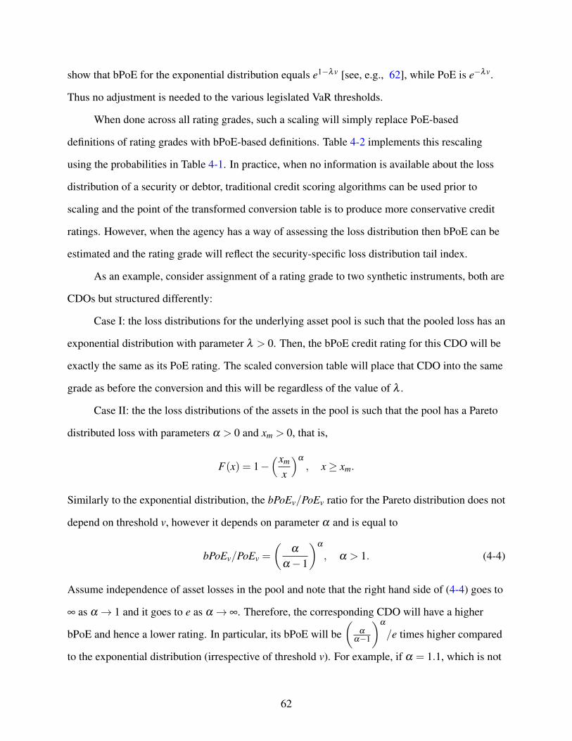
show that bPoE for the exponential distribution equals e1−λv [see, e.g., 62], while PoE is e−λv.

Thus no adjustment is needed to the various legislated VaR thresholds.

When done across all rating grades, such a scaling will simply replace PoE-based

definitions of rating grades with bPoE-based definitions. Table 4-2 implements this rescaling

using the probabilities in Table 4-1. In practice, when no information is available about the loss

distribution of a security or debtor, traditional credit scoring algorithms can be used prior to

scaling and the point of the transformed conversion table is to produce more conservative credit

ratings. However, when the agency has a way of assessing the loss distribution then bPoE can be

estimated and the rating grade will reflect the security-specific loss distribution tail index.

As an example, consider assignment of a rating grade to two synthetic instruments, both are

CDOs but structured differently:

Case I: the loss distributions for the underlying asset pool is such that the pooled loss has an

exponential distribution with parameter λ > 0. Then, the bPoE credit rating for this CDO will be

exactly the same as its PoE rating. The scaled conversion table will place that CDO into the same

grade as before the conversion and this will be regardless of the value of λ .

Case II: the the loss distributions of the assets in the pool is such that the pool has a Pareto

distributed loss with parameters α > 0 and xm > 0, that is,

F(x) = 1−(xm

x

)α

, x≥ xm.

Similarly to the exponential distribution, the bPoEv/PoEv ratio for the Pareto distribution does not

depend on threshold v, however it depends on parameter α and is equal to

bPoEv/PoEv =

(α

α−1

)α

, α > 1. (4-4)

Assume independence of asset losses in the pool and note that the right hand side of (4-4) goes to

∞ as α → 1 and it goes to e as α → ∞. Therefore, the corresponding CDO will have a higher

bPoE and hence a lower rating. In particular, its bPoE will be(

α

α−1

)α

/e times higher compared

to the exponential distribution (irrespective of threshold v). For example, if α = 1.1, which is not

62

unusual especially for financial returns on emerging markets, the bPoE will be more than 5 times

higher. Using the one-year ahead values from Tables 4-1 and 4-2, if this CDO used to be AA, it is

now BBB!

0 0.05 0.1 0.15 0.2 0.25 0.3 0.35 0.4 0.45 0.5

POE

2

2.1

2.2

2.3

2.4

2.5

2.6

2.7

bP

OE

/PO

E

0 0.5 1 1.5 2 2.5 3

x

2

2.1

2.2

2.3

2.4

2.5

2.6

2.7

bP

OE

/PO

E

Figure 4-4. Relationship between bPoE and PoE. Left graph shows the relationshipbetween PoEv(X) and bPoEv(X)/PoEv(X) for the standard normaldistribution. Right graph shows relationship between quantile v andbPoEv(X)/PoEv(X) for the standard normal distribution.

Table 4-2. Revised ratings for buffered probability of default.Rating \Time 1 2 3 4 5AAA 0.00 0.08 0.35 0.65 0.95AA 0.05 0.16 0.35 0.63 0.92A 0.16 0.41 0.71 1.09 1.50BBB 0.52 1.44 2.47 3.72 5.00BB 1.98 6.12 11.06 15.93 20.41B 10.25 23.27 34.41 43.00 49.66CCC/C 71.65 96.61 100.00 100.00 100.00Investment grade 0.27 0.76 1.30 1.98 2.66Speculative grade 10.33 20.22 28.81 35.75 41.43

In order to further illustrate the effect of switching from PoE to bPoE consider the case of

two assets, one with normally distributed losses with parameters µ = 10 and σ = 3 (Asset 1) and

another with log-normal losses with parameters m = 0.02852 and variance v = 1 (Asset 2).

Suppose that each asset defaults if the loss is greater than 18.7 (default threshold). Then,

probability of default of each asset is 0.018% and therefore, each will have an AA-rating.

However, the expected loss for Asset 1 in case of default is 19.6, while the expected loss for Asset

2 in case of default is 26.4. Clearly Asset 2 is a more risky investment but the ratings do not

63

differential between them. If we now turn to bPoE, Asset 1 has bPoE=0.049%, corresponding to

an AA-rating (unchanged), while Asset 2 has bPoE = 0.059%, giving it an A-rating. This is, of

course, the reflection of the fact that the loss distribution of Asset 2 has a heavier tail.

4.6 Uncovered Call Options Investment Strategy

We illustrate how bPoE-based ratings prevent overuse of uncovered call options investment

strategies similar to those employed in the industry around the time of the AIG debacle. The idea

is that the conventional credit rating incentivizes the strategies that load the book with upper

tranches of CDOs without appropriate hedging. This leads to accumulation of uncovered

exposure which is not reflected in the credit rating. Effectively, the tail of the loss distribution is

made arbitrary heavy and the credit rating fails to reflect this.

Consider the following simple model. Suppose that a portfolio manager sells a number of

uncovered call options with the same underlying asset and strike price K. Without loss of

generality, assume zero interest rates and let P(K) be the price of the option with strike price K.

We assume that the portfolio has no capital, except proceeds from selling the call options. The

portfolio manager sells nK = 1P(K) options so that the proceeds from the sale are equal to $1.

Given an underlying asset price ST at maturity time T , the call option payoff at time T equals

fK = maxST −K,0.

The portfolio will have a negative balance, when nK fK−1 > 0, which is defined to be

default. Thus, the default probability P(nK fK−1 > 0) is PoE of the random variable nK fK−1

with the threshold at 0.

Assume that St evolves over time according to the geometric Brownian motion

St = S0e(µ−σ2/2)t+σWt ,

where Wt is the Wiener process. Thus, price St is log-normally distributed with cumulative

distribution function

Ft(x) =12+

12

erf(

ln(x)−mt√2st

)

64

with parameters mt = lnS0 +(µ−0.5σ2)t and st = σ√

t, for each time instance t ∈ (0,T ] (see,

e.g., Chapter 14 in [63]).

Then, it is easy to show that the probability of default equals

P(nK fK−1 > 0) = P(

maxST −K,0> 1nK

)= P

(maxST −K− 1

nK

,− 1nK

> 0)

= P(

ST > K +1nK

)= 1−FT

(K +

1nK

).

Furthermore,

PoE0(nK fK−1) = P(nK fK−1 > 0)→ 0 as K→ ∞ . (4-5)

In other words, we can reduce PoE by simply increasing the strike price K. It is no surprise in this

setting, that top-notch ratings can be obtained using PoE-based credit rating by increasing the

exposure of the portfolio through a sufficiently high strike price.

Now consider the bPoE for nK fK−1 at the threshold value of 0. The probability density

function of random variable XK = nK fK−1 has a single atom located at point XK =−1 with

probability P(nK fK−1 =−1) = P(ST ≤ K). The cdf of XK ≥ x where x ∈ (−1,∞) is

P(XK ≥ x) = P(nK fK−1≥ x) = P(

fK ≥x+1

nK

)= P

(ST ≥

x+1nK

+K).

Thus, for values grater than -1, the distribution of XK is the same as log-normal distribution

corresponding to ST , however it is shifted left by K +1/nK and is scaled by nK .

In order to calculate bPoE0(XK) we need to consider two possibilities. In the first case,

when E [XKIXK >−1]≤ 0, the value bPoE0(XK) can be calculated using only the log-normal

part of the distribution of XK . In the second case, when E [XKIXK >−1]> 0, it is necessary to

take some fraction of the probability of the atom, in order to bring the conditional expectation

down to 0. Thus, in the second case, bPoE0(XK) is calculated as

bPoE0(XK) = P(XK >−1)+ p−1,

65

where p−1 is the fraction of the probability of the atom, such that

0 = E [XKIXK >−1]+ (−1)p−1. (4-6)

Because nK is always positive,

bPoE0(XK) = bPoE0(nK fK−1) = P( fK > 0)+ p−1 = P(ST > K)+ p−1 .

Note that IXK >−1= InK fK−1 >−1= IST > K. Then, from (4-6), we have

bPoE0(XK) = P(ST > K)+E [XKIXK >−1]

= P(ST > K)+E [(nK fK−1)IST > K]

= P(ST > K)+nKE [ fKIST > K]−P(ST > K)

= nKE [ fK] . (4-7)

From the fundamental theorem of asset pricing (see Chapter 14 in [63]) and our assumption

that interest rates (including risk free) are 0, we have that

nK =1

P(K)=

1E [ fK]

. (4-8)

Substituting the right-hand side of (4-8) in (4-7) we get

bPoE0(XK) = nKE [ fK] =1

E [ fK]E [ fK] = 1, (4-9)

so bPoE-based rankings would be informative of the extremely high riskiness of the strategy.

4.7 Application to Optimal Step-Up CDO Structuring

A significant advantage of bPoE-based ratings is the possibility they offer to solve to

optimality complicated portfolio optimization and structuring problems. This section discusses

the problem of CDO structuring in order to demonstrate this advantage with a practical example.

A CDO consists of a pool of assets generating a cash flow. This asset pool is repackaged in

a number of tranches with ordered priority on the collateral in the event of default. Each of these

tranches comes with a separate rating assigned to it. Top-quality tranches, often called senior

66

tranches, have the first priority on collateral payment in the event of default. They have a higher

rating compared to other tranches, often called mezzanine and equity tranches.

Each tranche has an attachment and detachment point that controls the amount of loss

absorbed by the tranche in the event of default. The detachment point of a given tranche is the

attachment point of the following upper tranche. A CDO tranche defaults when the cumulative

loss reaches its attachment point. At each time t, there is a set of attachment/detachment points

that determine the width of a tranche as illustrated in Figure 4-5. Traditionally, the tranche rating

is calculated based on the PoE of the loss using the attachment point of the tranche as a threshold.

Tranches are sold to investors as separate assets and the payoff (spread) of the tranche depends on

the assigned rating.

A CDO consisting of a pool of credit default swaps (CDSs) is called synthetic. CDS buyers

make payments (CDS spreads) every time period to the CDO originator. The CDO originator

“repackages” these spreads and makes payments (tranche spreads) to buyers of CDO tranches. A

tranche spread depends on an attachment point and is driven by the tranche rating.

We now show how the bPoE-based ratings can be used for structuring of synthetic CDOs.

Given a fixed pool of assets, a common objective pursued in structured finance is to select

positions in the pool of assets and optimal attachment points.

4.7.1 Optimal CDO Structuring with PoE-Based Ratings

We consider the optimization problem faced by an originator of a synthetic CDO: to find

such positions in a pool of CDSs and such CDO attachment points that result in maximum profit.

That is, we minimize the expected sum of discounted spread payments subject to constraints on

tranche ratings (to ensure CDO tranche spreads) and a constraint on the cost of the purchased

pool [see, e.g., 15, Problem B]. We solve this optimization problem for various costs of purchased

pool. The most profitable CDO has the largest difference between the received CDS spreads and

paid tranche spreads.

67

Figure 4-5. CDO attachment and detachment points

We start with describing the problem of calculating optimal attachment points assuming a

fixed pool of CDSs. Then, we extend the problem and include a CDS portfolio optimization

component.

Let M denote the number of tranches, T the number of time periods, Lt the loss at each time

t = 1, . . . ,T and sm the spread payment for each tranche m = 1, . . . ,M. The total payment for a

tranche with the given attachment/detachment points (xtm,x

tm+1) at time t can be written as follows

M

∑m=1

(xtm+1−max(xt

m,Lt))+sm . (4-10)

Given a discount rate r, the goal is to minimize the expected present value of the total future

payments with respect to tranche attachment points xt2, . . . ,x

tm

T

∑t=1

1(1+ r)t

M

∑m=1

E(xtm+1−max(xt

m,Lt))+sm . (4-11)

The lowest attachment point is assumed to be fixed at zero, xt0 = 0, t = 1, . . . ,T .

[15] proved that the objective function (4-11) has the following equivalent representation

T

∑t=1

1(1+ r)t

M

∑m=1

∆smE[(xtm+1−Lt)

+] , (4-12)

68

where ∆sm = sm− sm+1 . Being a sum of expectations of convex functions in attachment points

xtm , this representation is more attractive as it is convex in xt

m, which is a desirable property in

optimization.

By construction, each tranche in the CDO has a predefined rating. Let pm denote the

probability of default at any time point up to T , corresponding to a given tranche rating. Then, the

rating constraints on the tranche attachment points are written as follows

1−P(L1 ≤ x1m, . . . ,LT ≤ xT

m) ≤ pm m = 2, . . . ,M . (4-13)

These constraints bound default probabilities of tranches. Note that in (4-13) index m starts from

2 because the attachment point of the lowest tranche is fixed at zero. Additionally, the attachment

points should satisfy the monotonicity constraints

xtm ≥ xt

m−1 m = 3, . . . ,M; t = 1, . . . ,T. (4-14)

Let us denote by x = xtm

t=1,...,Tm=2,...,M the vector of attachment points. By combining

(4-12)-(4-14), we write the optimization problem as follows

minx

T

∑t=1

1(1+ r) t

M

∑m=1

∆smE[(xtm+1−Lt)

+] (4-15)

subject to the constraints

1−P(L1 ≤ x1m, . . . ,LT ≤ xT

m)≤ pm m = 2, . . . ,M (4-16)

xtm ≥ xt

m−1 m = 3, . . . ,M; t = 1, . . . ,T (4-17)

0≤ xtm ≤ 1 m = 2, . . . ,M; t = 1, . . . ,T (4-18)

Further we include optimization of the portfolio of CDSs into problem (4-15)-(4-18). Let K

denote the number of available CDSs. Let yk, k = 1, . . . ,K, denote the weight of the k-th asset in

the asset pool and ck the annual income spread payment of the CDS. Assume that the CDS

portfolio should obtain an annual spread of at least ζ , where ζ is a parameter. Let θ tk denote the

69

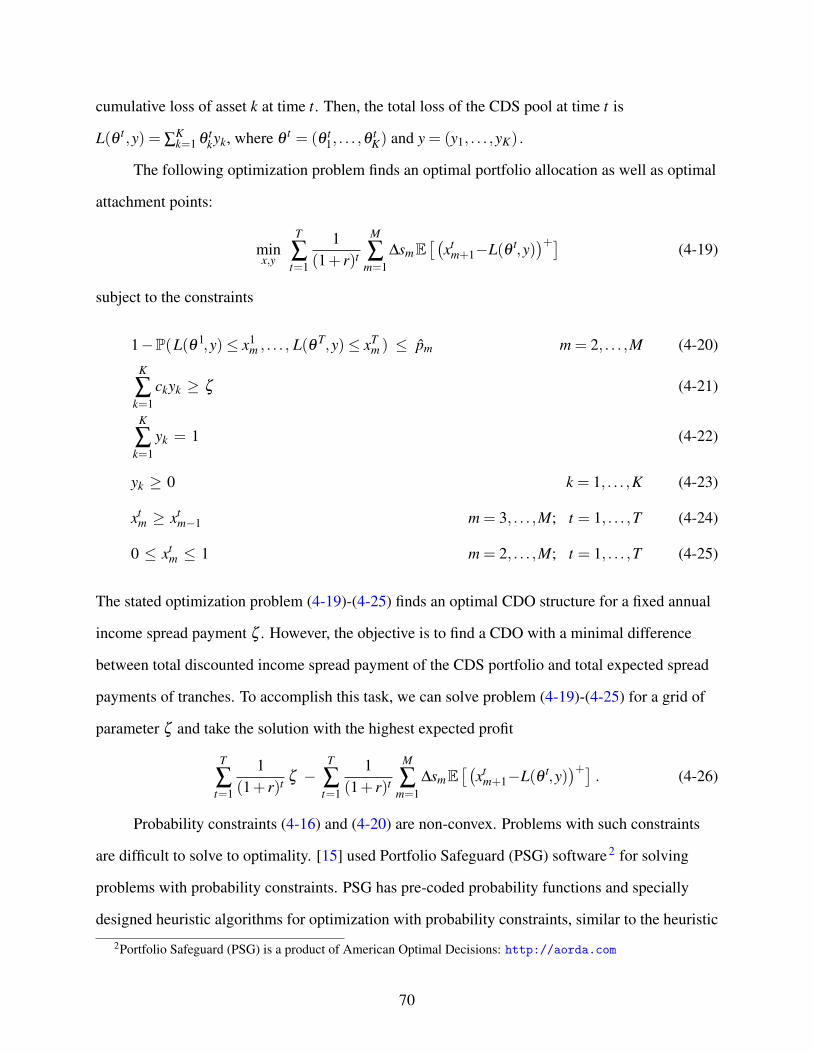
cumulative loss of asset k at time t. Then, the total loss of the CDS pool at time t is

L(θ t ,y) = ∑Kk=1 θ t

kyk, where θt = (θ t

1, . . . ,θtK) and y = (y1, . . . ,yK) .

The following optimization problem finds an optimal portfolio allocation as well as optimal

attachment points:

minx,y

T

∑t=1

1(1+ r)t

M

∑m=1

∆smE[(

xtm+1−L(θ t,y)

)+] (4-19)

subject to the constraints

1−P(L(θ 1,y)≤ x1m , . . . , L(θ T,y)≤ xT

m ) ≤ pm m = 2, . . . ,M (4-20)

K

∑k=1

ckyk ≥ ζ (4-21)

K

∑k=1

yk = 1 (4-22)

yk ≥ 0 k = 1, . . . ,K (4-23)

xtm ≥ xt

m−1 m = 3, . . . ,M; t = 1, . . . ,T (4-24)

0 ≤ xtm ≤ 1 m = 2, . . . ,M; t = 1, . . . ,T (4-25)

The stated optimization problem (4-19)-(4-25) finds an optimal CDO structure for a fixed annual

income spread payment ζ . However, the objective is to find a CDO with a minimal difference

between total discounted income spread payment of the CDS portfolio and total expected spread

payments of tranches. To accomplish this task, we can solve problem (4-19)-(4-25) for a grid of

parameter ζ and take the solution with the highest expected profit

T

∑t=1

1(1+ r)t ζ −

T

∑t=1

1(1+ r)t

M

∑m=1

∆smE[(

xtm+1−L(θ t,y)

)+]. (4-26)

Probability constraints (4-16) and (4-20) are non-convex. Problems with such constraints

are difficult to solve to optimality. [15] used Portfolio Safeguard (PSG) software 2 for solving

problems with probability constraints. PSG has pre-coded probability functions and specially

designed heuristic algorithms for optimization with probability constraints, similar to the heuristic

2Portfolio Safeguard (PSG) is a product of American Optimal Decisions: http://aorda.com

70

http://aorda.com

described by [64] for Value-at-Risk optimization. PSG provides reasonable solutions for these

non-convex problems, but does not guarantee optimality.

Data, codes and solutions for six simplified variants of problem (4-15)-(4-18) described in

detail in [15] are posted online 3; see Problems 1-6 and the description of the case study posted on

the website.

4.7.2 Optimal CDO Structuring with bPoE-Based Ratings

In this section we demonstrate how the non-convex risk management problems with PoE

constraints can be converted into convex problems with bPoE constraints. Specifically we

consider extensions of optimization problem (4-19)-(4-25) which find, in one shot, the optimal

attachment points of a CDO and the optimal portfolio component allocation. We emphasize that

this problem has not, until now, been solved to optimality.

Constraint (4-20) is equivalent to

PoE0

(max

L(θ 1,y)−x1

m , . . . , L(θ T,y)−xTm

)≤ pm , (4-27)

which defines a non-convex region for variables x,y. However, a similar constraint with bPoE

bPoE0

(max

L(θ 1,y)−x1

m , . . . , L(θ T,y)−xTm

)≤ pm (4-28)

defines a convex region, where pm is some scaled bound on probability. The convexity of the

feasible region of constraint (4-28) follows from the quasi-convexity of bPoE in random variable

and convexity of the function maxL(θ 1,y)−x1m , . . . , L(θ T,y)−xT

m

in (x,y) [see 48, Proposition

4.8]. More importantly, bPoE constraint (4-28) is more conservative compared to PoE constraint

(4-27) and the effect of this replacement is greater for loss distributions with fatter tails. Under the

assumption of an exponential tail, the following bPoE constraint is equivalent to (4-27)

bPoE0

(max

L(θ 1,y)−x1

m , . . . , L(θ T,y)−xTm

)≤ e pm , (4-29)

where e = 2.7182. However, generally the two constraints are not equivalent.

3Online Supplement “Case study: structuring step-up CDO” is available at http://uryasev.ams.stonybrook.edu/index.php/research/testproblems/financial_engineering/structuring-step-up-cdo/

71

http://uryasev.ams.stonybrook.edu/index.php/research/testproblems/financial_engineering/structuring-step-up-cdo/

http://uryasev.ams.stonybrook.edu/index.php/research/testproblems/financial_engineering/structuring-step-up-cdo/

An additional benefit is that bPoE and CVaR constraints are equivalent [see 48]. Constraint

(4-29) is equivalent to the following CVaR constraint

CVaR1−e pm

(max

L(θ 1,y)−x1

m , . . . , L(θ T,y)−xTm

)≤ 0 . (4-30)

bPoE is one minus the inverse function of CVaR, therefore, an appropriate confidence level in

CVaR constraint (4-30) is 1− e pm. CVaR-based objective functions and constraints are coded in

many software packages. For instance, MATLAB has a financial toolbox that included CVaR

functions.

In addition, it is worth mentioning that the probability function in the left hand side of

equations (4-20) and (4-27) is the high-dimensional CDF of random vector

L(θ,y) =(

L(θ 1,y) , . . . , L(θ T,y))

at point x, i.e.,

CDFL(θ,y)(x) = P(L(θ 1,y)≤ x1m , . . . , L(θ T,y)≤ xT

m )

= 1 − PoE0

(max

L(θ 1,y)−x1

m , . . . , L(θ T,y)−xTm

).

We can define buffered CDF of the random vector L(θ,y) at point x as follows

bCDFL(θ,y)(x) = 1 − bPoE0

(max

L(θ 1,y)−x1

m , . . . , L(θ T,y)−xTm

).

Therefore, convex constraint (4-28) is a constraint on buffered CDF bCDFL(θ,y)(x) and it is

equivalent to constraint (4-30) on CVaR.

Next we demonstrate the effect of replacing PoE with bPoE and CVaR in the CDO

structuring problem described in the previous section. We numerically solve problem

(4-19)-(4-25) with three types of risk constraints for tranches:

Problem PoE: problem (4-19)-(4-25) with PoE constraint (4-20);

Problem bPoE: problem (4-19)-(4-25) with PoE constraint (4-20) replaced by bPoE

constraint (4-29);

Problem CVaR: problem (4-19)-(4-25) with PoE constraint (4-20) replaced by CVaR

constraint (4-30).

72

Codes, data, and solutions for these three problems are posted online (see Problems 7-9).

We consider a CDO with 5 tranches (M = 5) using the data from [15]. The most “Senior”

tranche has the highest credit rating (AAA), followed by the “Mezzanine 1” (AA), “Mezzanine 2”

(A), “Mezzanine 3” (BBB) and finally “Equity” tranche (no rating). The planning horizon is 5

years (T = 5). The interest rate is assumed to be r = 7% and, for simplicity, discounting is done

in the middle of the year. With Standard and Poor’s credit ratings and corresponding default

probabilities from Table 4-1, maximum default probabilities for tranches are presented in Table

4-3 in column “PoE DP”. Column “bPoE DP” of Table 4-3 contains default probabilities based on

bPoE, see Table 4-2; column “Rating” shows ratings of the tranches.

Table 4-3. PoE and bPOE constraint right hand sides and corresponding ratings. “Tranche” =tranche name; “PoE DP” and “bPoE DP” = maximum default probability for a CDOtranche based on PoE and bPoE of attachment point; “Rating” = rating of tranche.Equity tranche does not have a rating.

Tranche PoE DP bPoE DP RatingSenior 0.35% 0.95% AAAMezzanine 1 0.34% 0.92% AAMezzanine 2 0.55% 1.50% AMezzanine 3 1.84% 5.00% BBB

In Table 4-3, Senior tranche has higher default probability than Mezzanine 1 tranche (both

PoE and bPoE), which is unusual but follows from the actual S&P default rates. A CDS pool is

the underlying asset for the considered CDO. Simulations of default scenarios for the CDSs in the

pool were done using Standard and Poor’s CDO Evaluator. The dataset contains a list of defaults

and recovery rates for CDSs in the pool for 3×105 scenarios. This number of scenarios is

considered adequate for low probability events, such as a default of the AAA Senior tranche.

For optimization we used AORDA PSG version 2.3, running on a Windows 10 PC, with

Intel Core i7-8550U CPU. We used the VANGRB PSG solver which minimizes a sequence of

quadratic programming problems by calling the GUROBI solver. We note that although problems

with bPoE and CVaR constraints are convex in decision variables, they are quite challenging from

the numerical perspective. A reduction to linear programming with additional variables results in

73

dimension exceeding 1.2×107 variables. PSG is capable of solving such problems to optimality

because it has pre-coded bPoE and CVaR functions with algorithms designed to solve such

problems. PSG also has a pre-coded PoE function and optimization problems with PoE functions

can be solved to optimality for problems with a small number of scenarios. However, for a large

number of scenarios, PSG uses a heuristic suggested by [64], which does not guarantee

optimality.

Table 4-4. Numerical results for CDO structuring problem with three types of risk constraints.Risk constraint Solving time (sec) Objective value Duality GapPoE 3223 544.54 N/AbPoE 286 545.78 10−5

CVaR 285 545.78 10−5

Table 4-4 reports solving time, minimal objective value and solution precision (Duality

Gap) for the problems with PoE, bPoE and CVaR risk constraints. First, we note that Problem

bPoE and Problem CVaR provide identical objective values and duality gaps. This is not

surprising as these two problems are equivalent. Also, we observe that changing the constraint

type from PoE to bPoE or CVaR leads to a significant improvement in solution time with a similar

objective value. The solving-time improvement is particularly remarkable as Problem bPoE and

Problem CVaR were solved to optimality (Duality Gap = 10−5) while there is no optimality

guaranty for Problem PoE (Duality Gap=N/A (not applicable)).

To illustrate the difference between PoE- and bPoE-based ratings, the dataset from [15] was

modified for 500 scenarios with a 50% default rate of each CDS in the CDO. These stressed

losses happen in the 5-th year of CDS payments and ensure that the tail of the loss distribution is

heavy. However, the probability of high losses for stressed scenarios is small:

500/(3×10−5) = 1.6×10−3 = 0.166%. This probability is about twice lower than the AAA

default probability of 0.35%, see Table 4-3.

As discussed earlier, this implies a significant difference between PoE- and bPoE-based

ratings and illustrates how bPoE ratings accurately account for heavy tails. The calculation results

74

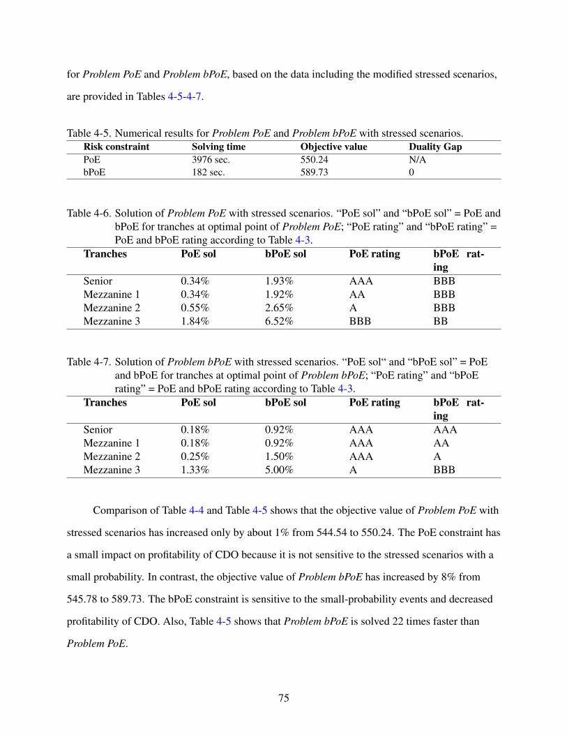
for Problem PoE and Problem bPoE, based on the data including the modified stressed scenarios,

are provided in Tables 4-5-4-7.

Table 4-5. Numerical results for Problem PoE and Problem bPoE with stressed scenarios.Risk constraint Solving time Objective value Duality GapPoE 3976 sec. 550.24 N/AbPoE 182 sec. 589.73 0

Table 4-6. Solution of Problem PoE with stressed scenarios. “PoE sol” and “bPoE sol” = PoE andbPoE for tranches at optimal point of Problem PoE; “PoE rating” and “bPoE rating” =PoE and bPoE rating according to Table 4-3.

Tranches PoE sol bPoE sol PoE rating bPoE rat-ing

Senior 0.34% 1.93% AAA BBBMezzanine 1 0.34% 1.92% AA BBBMezzanine 2 0.55% 2.65% A BBBMezzanine 3 1.84% 6.52% BBB BB

Table 4-7. Solution of Problem bPoE with stressed scenarios. “PoE sol“ and “bPoE sol” = PoEand bPoE for tranches at optimal point of Problem bPoE; “PoE rating” and “bPoErating” = PoE and bPoE rating according to Table 4-3.

Tranches PoE sol bPoE sol PoE rating bPoE rat-ing

Senior 0.18% 0.92% AAA AAAMezzanine 1 0.18% 0.92% AAA AAMezzanine 2 0.25% 1.50% AAA AMezzanine 3 1.33% 5.00% A BBB

Comparison of Table 4-4 and Table 4-5 shows that the objective value of Problem PoE with

stressed scenarios has increased only by about 1% from 544.54 to 550.24. The PoE constraint has

a small impact on profitability of CDO because it is not sensitive to the stressed scenarios with a

small probability. In contrast, the objective value of Problem bPoE has increased by 8% from

545.78 to 589.73. The bPoE constraint is sensitive to the small-probability events and decreased

profitability of CDO. Also, Table 4-5 shows that Problem bPoE is solved 22 times faster than

Problem PoE.

75

Table 4-6 demonstrates that PoE-based ratings do not reflect the increased riskiness coming

from the stressed scenarios. In this Table, “PoE sol” and “bPoE sol” stand for PoE and bPoE at the

solution of Problem PoE, respectively; “PoE rating” and “bPoE rating” stand for tranche ratings

calculated using PoE- and bPoE-based ratings, respectively, see Table 4-3. The PoE tranche

ratings in Table 4-6 coincide with the ratings in Table 4-3 of the original Problem PoE without the

stressed scenarios. However, the corresponding bPoE ratings in Table 4-6 are drastically lower

than the PoE ratings, reflecting the actual risk of the additional 500 stressed scenarios.

Finally, Table 4-7 shows the solution of Problem bPoE, similar to Table 4-6 showing the

solution of Problem PoE. Here, the CDO is calibrated using the bPoE rating constraints. Again,

the PoE-based ratings are severely inflated. In this case, the high PoE-based ratings can be

interpreted as the ratings that would have been required to correctly reflect the riskiness of the

additional stressed scenarios.

565 570 575 580 585 590 595540

560

580

600

620

640

660

680

POE constrained problem

bPOE constrained problem

Figure 4-6. Discounted CDO income compared to CDO payments. Thehorizontal axis is the total discounted income, over 5 years, payedby the CDS pool of the CDO (in basis points); the vertical axis isthe total discounted spread payments of the CDO (in basis points).

Now we return to the comparison of the solutions of Problem PoE and Problem bPoE for

the original dataset without stressed scenarios. The optimized objective values of these two

76

problems are very close, see Table 4-4. But there is still the question of whether using one or the

other constraint type generates significantly different cash flows. Figure 4-6 shows total

discounted spread payments of all tranches of the CDO (vertical axis in basis points) versus total

discounted income generated by the CDS pool underlying the CDO (horizontal axis in basis

points). The calculations are made for the two problems with ζ = 138,140,142,144,145 in

budget constraint (4-21). The solutions of the two problems are quite close, except at the highest

value of income generated by the CDS pool where the bPoE-based solution gives a higher spread.

We note that CDO profitability is measured by the difference between the horizontal and vertical

scale in the graph. We observe that the highest profitability is achieved for the smallest income

values. This means that for the considered dataset, the highest profitability is achieved by a

portfolio of CDSs with a low spread (and low default probability) for both the PoE- or

bPoE-constrained portfolios.

77

CHAPTER 5SUMMARY AND CONCLUSION

In the first part of this thesis we presented a new method for fitting mixture distributions

using CVaR distance. To assure that tails of the mixture distribution are as heavy as tails of

empirical distribution, we used CVaR constraints on the mixture distribution. We also considered

a cardinality constraint specifying that the number of distributions with nonzero weights in the

mixture is bounded by some constant. We proved that the CVaR of the mixture is a concave

function with respect to the weights of mixture. The case study illustrated fitting of the mixture

with CVaR constraints of 90%, 95%, 99%, 99.5% confidence levels. The case study demonstrated

that the suggested procedure ensures that the tails of the fitted mixture are as heavy as specified

by the constraints.

In the second part of the thesis we developed a multi-period investment model for

retirement portfolios. The parameters of the model represent a typical portfolio selection problem

solved in the beginning of retirement. The model maximizes expected estate value of an investor

subject to constraints on minimum cash outflows from the portfolio. Investment decisions are

based on adjustment rules implemented with kernel functions.

The case study showed performance of the model with pessimistic and optimistic sample

paths. In the pessimistic sample paths the market is assumed to enter a long term stagnation

modeled by subtracting 12% from all rates of returns of the stock/bond indexes considered for

investment. In this case it is optimal to invest a considerable portion of initial capital in annuities.

In the optimistic case the returns of stock/bond indexes are expected to remain similar to past

observations. In this case it is not beneficial to invest in the annuities, for the given model

parameters.

We defined a new cash outflow shortage measure called Expected Shortage Time (ETS).

The ETS calculates the number of years with shortage of cash outflows, given the retiree

minimum cash outflow requirements. The case study shows that even in the pessimistic sample

paths a retiree can have zero ETS for some small cash outflows, due to a significant investment in

the annuities.

78

The third part of the thesis presents a new approach to credit ratings based on the bPoE risk

function. bPoE-based ratings have a number of attractive features compared to PoE-based ratings.

They explicitly account for the magnitude of loss given default via their dependence on the tail of

the loss distribution. bPoE is a quasi-convex function in the random variable, which implies that

risk optimization problems are much easier to solve than PoE optimization problems.

We show that bPoE-based ratings address crucial inadequacies characterizing traditional

credit ratings. These include incentivizing excess risk exposure and encouraging credit risk

mispricing. We demonstrate bPoE’s advantages using several examples, including an uncovered

call options investment strategy with the incentive to open exceedingly large positions with low

default probabilities.

With CDO structuring problems, we argue that the new approach shows exceptional

promise from the computational perspective as it makes use of the quasi-convexity of bPoE-based

constraints and of the reduction to convex and linear programming. PoE-based ratings do not

capture high-value low-probability risks. bPoE-based ratings overcome this deficiency for loss

distributions with long tails.

79

REFERENCES

[1] S. Venkataraman, “Value at risk for a mixture of normal distributions: the use of quasi-Bayesian estimation techniques,” Economic Perspectives, no. Mar, pp. 2–13, 1997.

[2] D. Brigo and F. Mercurio, “Lognormal-mixture dynamics and calibration to marketvolatility smiles,” International Journal of Theoretical and Applied Finance, vol. 05, no. 04,pp. 427–446, 2002. [Online]. Available: https://doi.org/10.1142/S0219024902001511

[3] C. Alexander and E. Lazar, “Normal mixture garch(1,1): applications to exchange ratemodelling,” Journal of Applied Econometrics, vol. 21, no. 3, pp. 307–336, 2006.

[4] H. Permuter, J. Francos, and I. Jermyn, “A study of gaussian mixture models of color andtexture features for image classification and segmentation,” Pattern Recognition, vol. 39,no. 4, pp. 695 – 706, 2006, graph-based Representations. [Online]. Available:http://www.sciencedirect.com/science/article/pii/S0031320305004334

[5] A. P. Dempster, N. M. Laird, and D. B. Rubin, “Maximum likelihood from incomplete datavia the em algorithm,” Journal of the Royal Statistical Society. Series B (Methodological),vol. 39, no. 1, pp. 1–22, 1977.

[6] D. K. Kim and J. M. G. Taylor, “The restricted em algorithm for maximum likelihoodestimation under linear restrictions on the parameters,” Journal of the American StatisticalAssociation, vol. 90, no. 430, pp. 708–716, 1995. [Online]. Available:http://www.jstor.org/stable/2291083

[7] M. Jamshidian, “On algorithms for restricted maximum likelihood estimation,”Computational Statistics and Data Analysis, vol. 45, no. 2, pp. 137 – 157, 2004. [Online].Available: http://www.sciencedirect.com/science/article/pii/S0167947302003456

[8] K. Takai, “Constrained em algorithm with projection method,” Computational Statistics,vol. 27, no. 4, pp. 701–714, Dec 2012.

[9] P. Artzner, F. Delbaena, J. M. Eber, and D. Heath, “Coherent measures of risk,”Mathematical Finance, vol. 9, pp. 203–228, 1999.

[10] R. Rockafellar and S. Uryasev, “Conditional value-at-risk for general loss distributions,”Journal of Banking and Finance, vol. 26, pp. 1443–1471, 2002.

[11] R. Rockafellar and S. Uryasev, “Optimization of conditional value-at-risk,” The Journal ofRisk, vol. 2, pp. 21–41, 2000.

[12] K. Pavlikov and S. Uryasev, “Cvar norm and applications in optimization,” OptimizationLetters, vol. 8, pp. 1999–2020, 2014.

[13] A. Mafusalov and S. Uryasev, “Cvar (superquantile) norm: Stochastic case,” EuropeanJournal of Operational Research, vol. 249, pp. 200–208, 2016.

[14] K. Pavlikov and S. Uryasev, “Cvar distance between univariate probability distributions andapproximation problems,” Annals of Operations Research, vol. 262, no. 1, pp. 67–88, Mar2018. [Online]. Available: https://doi.org/10.1007/s10479-017-2732-8

80

https://doi.org/10.1142/S0219024902001511

http://www.sciencedirect.com/science/article/pii/S0031320305004334

http://www.jstor.org/stable/2291083

http://www.sciencedirect.com/science/article/pii/S0167947302003456

https://doi.org/10.1007/s10479-017-2732-8

[15] A. Veremyev, P. Tsyurmasto, and S. Uryasev, “Optimal structuring of cdo contracts:Optimization approach,” Journal of Credit Risk, vol. 8, 2012.

[16] A. Veremyev, P. Tsyurmasto, and S. Uryasev, “Case study: Structuring step up cdo.”[Online]. Available: http://www.ise.ufl.edu/uryasev/research/testproblems/financial engineering/structuring-step-up-cdo

[17] Case study: Fitting mixture models with cvar constraints. [Online]. Available:http://www.ise.ufl.edu/uryasev/research/testproblems/advanced-statistics/fitting-mixture-models-with-cvar/

[18] H. Markowitz, “Portfolio selection,” The Journal of Finance, vol. 7, pp. 77–91, 1952.

[19] P. Krokhmal, J. Palmquist, and S. Uryasev, “Portfolio optimization with conditionalvalue-at-risk objective and constraints,” The Journal of Risk, vol. 4, pp. 11–27, 2002.

[20] A. Chekhlov, S. Uryasev, and M. Zabarankin, “Portfolio optimization with drawdownconstraints, b. scherer (ed.) asset and liability management tools, risk books, london,” 2003.

[21] A. Chekhlov, S. Uryasev, and M. Zabarankin, “Drawdown measure in portfoliooptimization,” International Journal of Theoretical and Applied Finance, vol. 8, pp. 13–58,2005.

[22] M. Zabarankin, K. Pavlikov, and S. Uryasev, “Capital asset pricing model (capm) withdrawdown measure,” European Journal of Operational Research, vol. 234, pp. 508–517,2014.

[23] R. C. Merton, “Lifetime portfolio selection under uncertainty: The continuous-time case,”The Review of Economics and Statistics, vol. 51, pp. 247–257, 1969.

[24] R. C. Merton, “Optimum consumption and portfolio rules in a continuous-time model,”Journal of Economic Theory, vol. 3, pp. 373–413, 1971.

[25] P. A. Samuelson, “Lifetime portfolio selection by dynamic stochastic programming,” TheReview of Economics and Statistics, vol. 51, pp. 239–246, 1969.

[26] N. A. Rizal and S. K. Wiryono, “A literature review: Modelling dynamic portfolio strategyunder defaultable assets with stochastic rate of return, rate of inflation and credit spreadrate,” GSTF Journal on Business Review (GBR), vol. 4, no. 2, 2015.

[27] J. M. Mulvey and B. Shetty, “Financial planning via multi-stage stochastic optimization,”Computers and Operations Research, vol. 31, no. 1, pp. 1–20, 2004.

[28] J. M. Mulvey and H. Vladimirou, “Stochastic network programming for financial planningproblems,” Management Science, vol. 38, no. 11, pp. 1642–1664, 1992.

[29] D. Shang, V. Kuzmenko, and S. Uryasev, “Cash flow matching with risks controlled bybuffered probability of exceedance and conditional value-at-risk,” Annals of OperationsResearch, pp. 1–14, 2016.

81

http://www.ise.ufl.edu/uryasev/research/testproblems/financial_engineering/structuring-step-up-cdo

http://www.ise.ufl.edu/uryasev/research/testproblems/financial_engineering/structuring-step-up-cdo

http://www.ise.ufl.edu/uryasev/research/testproblems/advanced-statistics/ fitting-mixture-models-with-cvar/

http://www.ise.ufl.edu/uryasev/research/testproblems/advanced-statistics/ fitting-mixture-models-with-cvar/

[30] E. Bogentoft, H. Romeijn, and S. Uryasev, “Asset/liability management for pension fundsusing cvar constraints,” The Journal of Risk Finance, vol. 3, no. 1, pp. 57–71, 2001.

[31] G. C. Calafiore, “Multi-period portfolio optimization with linear control policies,”Automatica, vol. 44, no. 10, pp. 2463 – 2473, 2008.

[32] Y. Takano and J. Gotoh, “Multi-period portfolio selection using kernel-based control policywith dimensionality reduction,” Expert Systems with Applications, vol. 41, pp. 3901–3914,2014.

[33] W. K. Sjostrum, “The aig bailout,” Washington and Lee Law Review, vol. 66, pp. 941–991,2009.

[34] J. Coval, J. Jurek, and E. Stafford, “The economics of structured finance,” Journal ofEconomic Perspectives, vol. 23, pp. 3–25, 2009.

[35] D. Zimmer, “The role of copulas in the housing crisis,” The Review of Economics andStatistics, vol. 94, pp. 607—-620, 2012.

[36] A. Ashcraft, P. H. P. Goldsmith-Pinkham, and J. Vickery, “Credit ratings and security pricesin the subprime mbs market,” The American Economic Review, vol. 101, no. 3, pp. 115–119,2011.

[37] P. Bolton, X. Freixas, and J. Shapiro, “The credit ratings game,” The Journal of Finance,vol. 67, no. 1, pp. 85–111, 2012.

[38] M. Dilly and T. Mahlmann, “Is there a “boom bias” in agency ratings?” Review of Finance,vol. 20, no. 3, pp. 979–1011, 2016.

[39] A. Alp, “Structural shifts in credit rating standards,” The Journal of Finance, vol. 68, no. 6,pp. 2435–2470, 2013.

[40] E. I. Altman and H. A. Rijken, “How rating agencies achieve rating stability,” Journal ofBanking and Finance, vol. 28, no. 11, pp. 2679 – 2714, 2004.

[41] J. D. Amato and C. H. Furfine, “Are credit ratings procyclical?” Journal of Banking andFinance, vol. 28, no. 11, pp. 2641 – 2677, 2004.

[42] R. P. Baghai, H. Servaes, and A. Tamayo, “Have rating agencies become more conservative?implications for capital structure and debt pricing,” The Journal of Finance, vol. 69, no. 5,pp. 1961–2005, 2014.

[43] C. C. Opp, M. M. Opp, and M. Harris, “Rating agencies in the face of regulation,” Journalof Financial Economics, vol. 108, no. 1, pp. 46 – 61, 2013.

[44] J. He, J. Qian, and P. E. Strahan, “Are all ratings created equal? the impact of issuer size onthe pricing of mortgage-backed securities,” The Journal of Finance, vol. 67, no. 6, pp.2097–2137, 2012.

82

[45] B. Heski and J. Shapiro, “Ratings quality over the business cycle,” Journal of FinancialEconomics, vol. 108, no. 1, pp. 62 – 78, 2013.

[46] D. Kisgen, “Credit ratings and capital structure,” Journal of Finance, vol. 61, no. 3, pp.1035–1072, 2006.

[47] D. Kisgen, “The impact of credit ratings on corporate behavior: Evidence from moody’sadjustments,” Journal of Corporate Finance, vol. 58, pp. 567–582, 2019.

[48] A. Mafusalov and S. Uryasev, “Buffered probability of exceedance: Mathematical propertiesand optimization,” SIAM Journal on Optimization, vol. 28, no. 2, pp. 1077–1103, 2018.

[49] R. Rockafellar, “Safeguarding Strategies in Risky Optimization,” in Presentation at theInternational Workshop on Engineering Risk Control and Optimization, Gainesville, FL,2009.

[50] R. Rockafellar and J. Royset, “On buffered failure probability in design and optimization ofstructures,” Reliability Engineering and System Safety, vol. 95, no. 5, pp. 499–510, 2010.

[51] J. Davis and S. Uryasev, “Analysis of tropical storm damage using buffered probability ofexceedance,” Natural Hazards, 2016.

[52] M. Norton, A. Mafusalov, and S. Uryasev, “Cardinality of upper average and its applicationto network optimization,” SIAM Journal on Optimization, vol. 28, no. 2, pp. 1726–1750,2018.

[53] M. Norton and S. Uryasev, “Maximization of auc and buffered auc in binary classification,”Mathematical Programming, vol. 174, pp. 575–612, 2018.

[54] N. Norton, A. Mafusalov, and S. Uryasev, “Soft margin support vector classification asbuffered probability minimization,” Journal of Machine Learning Research, no. 18, pp.1–43, 2017.

[55] S. Trueck and S. Rachev, Rating Based Modeling of Credit Risk, 2009.

[56] D. Vazza and N. W. Kraemer, “Standard and poor’s global ratings. 2015 annual globalcorporate default study and rating transitions,” 2016.

[57] R. C. Merton, “On the pricing of corporate debt: The risk structure of interest rates,” Journalof Finance, vol. 29, pp. 449–470, 1974.

[58] R. Ibragimov, “Portfolio diversification and value at risk under thick-tailedness,”Quantitative Finance, vol. 9, no. 5, pp. 565–580, 2009.

[59] R. Ibragimov and A. Prokhorov, “Heavy tails and copulas: Limits of diversificationrevisited,” Economics Letters, vol. 149, pp. 102 – 107, 2016.

[60] C.-H. Hung, A. Banerjee, and Q. Meng, “Corporate financing and anticipated credit ratingchanges,” Review of Quantitative Finance and Accounting, vol. 48, no. 4, pp. 893–915,2017.

83

[61] M. Wojewodzki, W. Poon, and J. Shen, “The role of credit ratings on capital structure and itsspeed of adjustment: an international study,” European Journal of Finance, vol. 24, no. 9,pp. 735–760, 2018.

[62] A. Mafusalov, A. Shapiro, and S. Uryasev, “Estimation and asymptotics for bufferedprobability of exceedance,” European Journal of Operational Research, no. 270, pp.826–836, 2018.

[63] J. Hull, Options, Futures, and other Derivatives (7 ed.). Pearson, 2009.

[64] N. Larsen, H. Mausser, and S. Uryasev, Algorithms for Optimization of Value-At-Risk.Springer, 2002, pp. 19–46.

84

BIOGRAPHICAL SKETCH

Giorgi Pertaia received bachelor’s and master’s degrees in business administration with

specialization in Quantitative Finance from Georgian-American university in Tbilisi, Georgia.

During his master’s, Giorgi worked as a data analyst in the Internal Audit department of

Bank of Georgia in Tbilisi, Georiga. There he was in charge of developing statistical models for

various internal audit teams.

In 2016, Giorgi joined doctoral program at the University of Florida. Giorgi completed his

Doctor of Philosophy in Operations Research from the University of Florida in 2020. Giorgi’s

research interests include stochastic optimization, machine learning and financial engineering.

85

c 2020 Giorgi Pertaia - ufdcimages.uflib.ufl.edu

Documents

Transcript of c 2020 Giorgi Pertaia - ufdcimages.uflib.ufl.edu