c⃝ 2015 TIANQIN SHI

THREE ESSAYS ON PRODUCT DESIGN FOR THE ENVIRONMENT

BY

TIANQIN SHI

DISSERTATION

Submitted in partial fulfillment of the requirements

for the degree of Doctor of Philosophy in Business Administration

in the Graduate College of the

University of Illinois at Urbana-Champaign, 2015

Urbana, Illinois

Doctoral Committee:

Professor Dilip Chhajed, Co-Chair

Professor Nicholas C. Petruzzi, Co-Chair

Professor Zhixi Wan, University of Oregon

Professor Michael K. Lim

ABSTRACT

Design is a powerful instrument by which the world is forged to satisfy

the needs of mankind. As the awareness and pursuit of sustainability in-

creases, we have seen the transition from “design for needs” to “design for

environment”. Design for the Environment (DfE) requires manufacturers to

focus on conserving and reusing resources, minimizing waste, and reducing

hazard during a design process. DfE includes, but not limited to Design

for Recovery and Benign by Design. Manufacturers are facing the challenge

and opportunity of incorporating DfE into their businesses. Eco-conscious

product design is critical for the success of businesses, and, therefore, has

been an important research focus. This dissertation presents a design ap-

proach to help manufacturers maximize profits through optimal eco-conscious

product design, and to seek insights for policy makers and managers into

inducing product design for the environment. The focus of this dissertation

is the interaction between product design for the environment with market

segmentation, inter-divisional coordination, and regulatory policies.

This dissertation presents two studies on Design for Recovery. The first

study analyzes the effects of remanufacturable product design on market

segmentation and trade-in prices. By identifying the system and market

parameters under which it is optimal for a manufacturer to design a remanu-

facturable product, the study demonstrates that entering a remanufactured-

goods market in and of itself does not necessarily translate into environmental

friendliness. In addition, this study develops and compares several measures

of environmental efficiency, and concludes that emissions per revenue can

serve as the best proxy for emissions as a metric for measuring overall

environmental stewardship.

The second study investigates the impact of decentralization of manu-

facturing and remanufacturing operations within a firm on product design,

pricing, and profitability, and seeks inter-divisional incentive mechanism to

ii

achieve firm-wide coordination. This study shows that decentralization and

divisional conflict not only result in lower firm profit and product sales,

but also create a hurdle for remanufacturable product design. Thus, an

inter-divisional incentive mechanism is suggested to facilitate coordination

between two profit-maximizing divisions. The study signifies a two-part

coordination scheme (a transfer price and a fixed lump sum), through which a

decentralized firm can achieve first-best total profit and production quantity;

in addition, the manufacturing division is incentivized to design new products

to be remanufacturable.

The last study focuses on Benign by Design. In this essay, an innova-

tive pharmaceutical company decides whether to adopt green pharmacy in

response to the regulatory policy of the pharmaceutical stewardship and/or

patent term extension, as well as the competition from a generic company.

One the one hand, the patent term extension can encourage the innovative

company to invest in green pharmacy, and the regulator can induce green

pharmacy with short extended term when market competition is intensive.

On the other hand, a pharmaceutical company will neither go green nor bear

all the compliance cost in the presence of the take-back regulation because the

compliance cost is traditionally independent of the choice of green pharmacy.

Results show that although adding the take-back regulation on top of the

patent term extension generally reduces firm profit and requires a longer

term extension, such combined policy can excel the single policy of patent

term extension under certain circumstances. In addition, a modified take-

back policy that associates compliance cost with the firm’s choice of green

pharmacy is better than the patent term extension when the competition

intensity is relatively high.

iii

To my parents and husband, for their love and support.

To our only planet.

iv

ACKNOWLEDGMENTS

First and foremost, I would like to express sincere gratitude to my co-advisors

Professor Dilip Chhajed and Professor Nicholas C. Petruzzi for sharing with

me their expertise, vision and passion for research, and for showing me the

ropes in teaching during my entire Ph.D. study. I deeply appreciate that

they believe in me and devoted many evenings, weekends and lunch hours

to helping me. This dissertation would not have been possible without their

step-by-step guidance and unparalleled support.

I would also like to give my profound thanks to Professor Zhixi Wan

and Professor Michael Lim for their guidance and support, for serving on

my doctoral committee and for invaluable comments and suggestions in the

preparation of this dissertation.

Over the past five years, it has been my great honor to work with the

faculty of Operations Management (Process Management) in the Department

of Business Administration, UIUC: Prof. Anupam Agrawal, Prof. Gopesh

Anand, Prof. Dharma Kwon, Prof. Fataneh Taghaboni-Dutta, Prof. Han

Ye, and Dr. Meng Li. Working with them has been an invaluable and

enlightening experience.

My thanks also go to my colleagues and friends, in particular to all the

former and current students in the BA Department: Kunpeng Li, Chongqi

Wu, Wenjun Gu, Wenxin Xu, Karthik Murali, Youngsoo Kim, Xuefeng Liu,

Ying Xiao, Ya Tang, Duo Jiang, Kezhou Wang, Yifan Wei and Yaxian Xie.

Big thanks to my officemate, Wenxin, for helping me like a sister. I am

also very thankful to my other friends, including, Chen Yao, Cong Zhang,

Bing Zuo, Shuoyuan He, Qian Yin, Qingzhou Luo, Qingxi Li, Yu Qian,

among others, for making my stay at Urbana-Champaign a memorable one.

I would also like to extend my heartfelt thanks to my previous advisor and

colleagues in China, Professor Peng Tian and Professor Guohua Wan for

their continuing support and encouragement.

v

Last but not least, I want to thank my parents, including my in-laws,

and my husband for their unconditional love, gracious understanding, and

boundless support in all the ways in my life. They have been my inspiration

and motivation for moving my study and career forward. My grandma,

who rests in peace, shares credit on every goal I achieve. I dedicate this

dissertation to them.

Thank you all very much.

vi

TABLE OF CONTENTS

CHAPTER 1 INTRODUCTION . . . . . . . . . . . . . . . . . . . . 11.1 Design for Recovery and Benign by Design . . . . . . . . . . . 11.2 Motives for DfE . . . . . . . . . . . . . . . . . . . . . . . . . . 21.3 Barriers to DfE . . . . . . . . . . . . . . . . . . . . . . . . . . 41.4 The Objective and the Plan . . . . . . . . . . . . . . . . . . . 6

CHAPTER 2 EFFECTS OF REMANUFACTURABLE PROD-UCT DESIGN ON MARKET SEGMENTATION AND THEENVIRONMENT . . . . . . . . . . . . . . . . . . . . . . . . . . . . 92.1 Introduction . . . . . . . . . . . . . . . . . . . . . . . . . . . . 92.2 Relation to Literature . . . . . . . . . . . . . . . . . . . . . . 132.3 Assumptions and Models . . . . . . . . . . . . . . . . . . . . . 152.4 Analysis . . . . . . . . . . . . . . . . . . . . . . . . . . . . . . 232.5 Environmental Impact . . . . . . . . . . . . . . . . . . . . . . 342.6 Conclusion . . . . . . . . . . . . . . . . . . . . . . . . . . . . . 41

CHAPTER 3 THE INTER-DIVISIONAL COORDINATION OFMANUFACTURING AND REMANUFACTURING OPERA-TIONS IN A CLOSED-LOOP SUPPLY CHAIN . . . . . . . . . . . 443.1 Introduction . . . . . . . . . . . . . . . . . . . . . . . . . . . . 443.2 Related Literature . . . . . . . . . . . . . . . . . . . . . . . . 483.3 The Models . . . . . . . . . . . . . . . . . . . . . . . . . . . . 513.4 Inter-Divisional Coordination . . . . . . . . . . . . . . . . . . 623.5 Conclusions . . . . . . . . . . . . . . . . . . . . . . . . . . . . 69

CHAPTER 4 THE EFFECTS OF PATENT TERMEXTENSIONAND PHARMACEUTICAL STEWARDSHIP PROGRAM ONGREEN PHARMACY . . . . . . . . . . . . . . . . . . . . . . . . . 734.1 Introduction . . . . . . . . . . . . . . . . . . . . . . . . . . . . 734.2 Relation to Literature . . . . . . . . . . . . . . . . . . . . . . 784.3 Green Pharmacy, Patent Term Extension, and Take-back

Regulation Defined . . . . . . . . . . . . . . . . . . . . . . . . 804.4 Patent Term Extension and Model Solutions . . . . . . . . . . 844.5 The Role of Take-back Regulations . . . . . . . . . . . . . . . 904.6 Effects of Green Pharmacy on the Compliance Cost . . . . . . 95

vii

4.7 Conclusion . . . . . . . . . . . . . . . . . . . . . . . . . . . . . 101

CHAPTER 5 CONCLUSION . . . . . . . . . . . . . . . . . . . . . . 107

APPENDIX A APPENDIX FOR CHAPTER 2 . . . . . . . . . . . . 111

APPENDIX B APPENDIX FOR CHAPTER 3 . . . . . . . . . . . . 115

APPENDIX C APPENDIX FOR CHAPTER 4 . . . . . . . . . . . . 128

REFERENCES . . . . . . . . . . . . . . . . . . . . . . . . . . . . . . . 132

viii

CHAPTER 1

INTRODUCTION

“Rethinking the future: It is a profound challenge, at the end of an era of

cheap oil and materials to rethink and redesign how we produce and consume;

to reshape how we live and work, or even to imagine the jobs that will be

needed for transition.”

– Dame Ellen Patricia MacArthur.

1.1 Design for Recovery and Benign by Design

Design is one of the most powerful, inspiring, and enlightening instrument by

which the world is forged to satisfy the needs of mankind. As the awareness

and pursuit of sustainability increases, manufacturers are faced with the

challenge and opportunity of conducting green businesses, which drives the

transition from a “design for needs” to a “design for environment”. Design

for the Environment (DfE) is “a design process that must be considered

for conserving and reusing the earth’s scarce resources; where energy and

material consumption is optimized, minimal waste is generated and output

waste streams from any process can be used as the raw materials of another”

(Billatos and Basaly 1997). According to United Nations Economic and

Social Commission for Western Asia (ESCWA 2014), one of the central

concepts of DfE is the design for reuse or disposal. Product design is the

beginning of the life of a product, and it occupies great importance in terms

of environmental impact of the product from cradle (raw materials) to its

grave (recovery or disposal).

In end-of-life recovery, part of unwanted products become useful compo-

nents of other products (Fitzgerald et al. 2007). End-of-life recovery can

be achieved by various means, such as reuse, reconditioning, refurbishing,

remanufacturing, and recycling. Reuse and reconditioning require very few

1

reprocessing operations; reuse involves almost no value-adding treatments

while reconditioning requires minor value-adding treatments of cleaning, lu-

bricating, or polishing. Refurbishing and remanufacturing both include re-

placement of used parts; a remanufactured product is built with upgraded

parts while a refurbished product is built with parts that maintain the

original specifications (Kwak 2012). Recycling is the simplest but the least

resource-efficient form of recovery. The unwanted products are usually de-

formed so that raw materials can be extracted to produce different products.

Among these five forms of recovery, remanufacturing and refurbishing rely

heavily on the ease of inspection, cleaning, and disassembly (Sundin and

Bras 2005). It is evident that the difficulties in inspection, cleaning, and

disassembly can only be lowered or removed if products are designed for

remanufacturing and refurbishing. Therefore, Chapter 2 and 3 of this disser-

tation mainly focus on the design for remanufacturing.

End-of-life recovery is profitable when the residual value of unwanted

products are high. If the residual value is small, unwanted products are

disposed rather than recovered. The process of disposal generates negative

environmental impacts by potentially consuming energy, releasing emissions,

and contaminating surface and waters. Although efforts have been made to

reduce such impacts through end-of-pipe-control approach, it is always better

to prevent waste through benign design than to treat or clean up waste

afterwards. For example, green chemistry emphasizes the design of safer

chemicals (minimize the toxicity of chemical products), design for degrada-

tion (chemicals break down easily and do not persist in the environment), and

design for energy efficiency (minimize the energy requirements of chemical

processes) (Anastas and Warner 1998). Similarly, green pharmacy is the

design of pharmaceutical products and processes that eliminates or reduces

the use and generation of hazardous substances (EEA 2010). To achieve green

chemistry and green pharmacy, design for benignity is key. Thus, Chapter 4

studies several issues concerning a “benign-by-design” approach.

1.2 Motives for DfE

The transition from a “design for needs” to a “design for environment”

can be traced back to the early 1970s (Madge 1993). Today, Design for

2

the Environment (DfE), along with Green Design (GD), Environmentally

Conscious Design (ECD) and EcoDesign, is becoming a common practice in

many manufacturing and service industries (Giudice et al. 2006). Economic

profitability and environmental legislations are, among others, the key drivers

for DfE.

Profitability is the ultimate motivation for DfE, enabling manufacturers

to control cost, charge green premium and expand market. In many cases,

remanufacturing operations can be less expensive and more environmentally

friendly than manufacturing operations for manufacturers (Wu 2012). For

example, a remanufactured alternator offers 50% cost saving and 60-70%

energy and material consumption as compared to a new product (Fatimah

et al. 2013). However, products that are not designed to be easily remanu-

factured could result in very high costs, which makes remanufacturing barely

profitable (Sundin 2001, Kerr and Ryan 2001, Franke et al. 2006).

Not only does DfE help manufacturers to lower cost, it also allows compa-

nies to segment customers and practice price differentiation. Bhattacharya

and Sen (2003, 2004) pointed out that customers tend to establish strong and

committed relationship with companies and products that “help them satisfy

one or more important self-definitional needs”. Surveys and studies indicate

that some customers (usually with more psychological benefits obtained from

purchasing a sustainable item) are willing to pay a green premium on eco-safe

products (Cremer and Thisse 1999, Chen 2001, Sengupta 2012). As a result,

DfE helps transform the end-of-life operations from a “cost center” to a new

“revenue center” (Guide Jr and Van Wassenhove 2009).

Moreover, DfE creates a bigger pie for manufacturers as businesses and

market opportunities expand. For example, offering remanufactured prod-

ucts is an approach that can attract new end-customers by expanding product

lines to include less expensive alternative. BMW Exchange Part offers re-

manufactured components at a price 30-50% cheaper than new counterparts

(Thierry et al. 1995). By selling recovered products at a low price, manufac-

turers can attract consumers who would otherwise not purchase (Debo et al.

2005). Meanwhile, according to Cone Corporate Citizenship Study (2002),

84% Americans reported that they would switch brands to one associated

with a good cause, given similar price and quality. Therefore, manufacturers

can employ DfE to maintain its market share or gain a larger share. The

U.S. Environmental Protection Agency (EPA), who promotes the Design for

3

the Environment Program, also demonstrates this possible boundary:

“Companies that have invested in safer chemistry and earned the (EPA

Design for the Environment) label have entered an expanding marketplace

for sustainable products. These companies can look forward to growing

their businesses and adding green jobs to the economy. Participants in

the green marketplace include major retailers, such as Wal-Mart, Safeway,

Home Depot, and Target, which have given special status to Design for the

Environment-labeled products, and government purchasers who are increas-

ingly specifying the Design for the Environment label in their purchasing

requirements.”

– EPA Design for the Environment (http://www.epa.gov/dfe/faqs.html)

Environmental legislation has also been identified as a motivator for “de-

sign for environment”. Environmental legislation influences product design

in various ways. First, regulations, such as the Restriction of Hazardous

Substances (RoHS) Directive and recycled-content mandates, instigate de-

sign changes by prohibiting or restricting the use of some substances (Tof-

fel 2003). Second, take-back requirements, such as Waste Electrical and

Electronic Equipment (WEEE) Directive and End of Life Vehicle (ELV)

Directive, motivate manufacturers to modify product design such that end-

of-life product recovery becomes profitable or end-of-life product disposal

becomes easy and safe. This can be achieved, for example, by adopting easy-

disassembly or ready-recycling product and process design (Toffel 2004). A

list of Product Stewardship and Extended Producer Responsibility (EPR),

also called “Producer Takeback”, can be found at http://www.calrecycle.

ca.gov/epr/PolicyLaw/default.htm#World. Third, legislation on landfill

taxes, energy taxes, recycling subsidies and emissions trading encourages

manufacturers to design or redesign products and process in order to reduce

the consumption of energy and materials, or to minimize pollution and waste

(Calcott and Walls 2000, 2005, Plambeck and Wang 2009).

1.3 Barriers to DfE

Although the transition from a “design for needs” to a “design for en-

vironment” was initiated more than four decades ago, many managerial

4

decisions fail to follow the paradigms of sustainability (Flannery and May

2000, Seitz 2007). As a case in point, although Caterpillar undertook both

manufacturing and remanufacturing operations, its engine design priorities

were still largely governed by the needs of the manufacturing process (Stahel

1995). There are three types of barriers to the growth of DfE: (1) high cost,

(2) perceived value, and (3) cannibalization and competition.

In order to take advantage of the cost savings, manufacturers have to

design and produce products to be refurbishable or remanufacturable, which

could require costly materials and advanced technology (Lee and Bony 2008).

The cost saving from DfE may not always justify the additional expenses

on materials and technology. Moreover, original equipment manufacturers

(OEMs) need to pay higher prices for take-back operations and face strong

variations in quality, quantity and time of returned products (Guide Jr

and Van Wassenhove 2001), which can make DfE unattractive. DfE meets

extreme obstacle when the residual value of end-of-life products is nominal

and the environmental legislation to encourage responsible behavior is not

available.

DfE relies on the market demand and profitability. Recovered products

may not be well received by consumers because these products are associated

with lower quality as compared to new products (Guide Jr and Li 2010). Con-

sequently, a consumer’s willingness-to-pay (WTP) for a recovered product is

generally less than the WTP for a new counterpart, which drives down both

demand and profit of DfE. Furthermore, customers are not always strategic

in the sense that they do not consider life cycle costs of products (Gray and

Charter 2007). DfE may result in higher price but allows easy replacement

of parts and components, which could be beneficial to the consumers, in the

long run. Customers, however, may only compare the current price without

taking into account the future benefits.

The potential for cannibalization and competition is another major barrier

that prevents manufacturers to implement DfE. From one point of view,

selling refurbished or remanufactured products could cause extensive canni-

balization to the new products, hence impeding the profitability (Thomas

2003, Ferguson and Toktay 2006, Atasu et al. 2008). In such a case, manu-

facturers would rather not invest in designing products to be refurbishable or

remanufacturable. From another point of view, even if OEM do not tap into

remanufactured-goods markets by themselves, third-party remanufacturers,

5

who only target at the secondary markets, could collect, recover and resell

used products (Ferguson and Toktay 2006, Oraiopoulos et al. 2012). The

external competition from recovered products may drive OEMs to ‘clean the

market’ so that independents do not have access to cores (Seitz 2007). Even

worse, OEMs will eliminate the secondary market by deliberately designing

products that are exceedingly difficult to take apart and recover. Gell (2008)

reported that toner cartridge OEMs deter remanufacturers by using anti

reuse devices (ARUDs) such as sonic welding and unnecessary adhesive tapes,

techniques that restrict toner cartridges to being either single-cycle or short-

life.

1.4 The Objective and the Plan

The principal goals of this dissertation are: (1) to explore the relationship

among Design for the Environment (DfE), profitability and environment,

and (2) to develop and examine mechanisms that facilitate DfE. Improving

the adopting of DfE is only achievable by understanding the economic and

environmental implications of DfE. However, such implications have not been

clear, which hinders the application of DfE. Also, as discussed in Section 1.3,

barriers to both Design for Recovery and Design for Benignity widely exist,

and questions still linger over how to induce DfE. Thus, the contribution

of the work is two-fold. On the one hand, this dissertation provides clear

understanding of Design for the Environment by integrating the perspectives

on profitability and environment. On the other hand, this dissertation seeks

insights for regulators and managers on how to incent manufacturers or

design decision makers to implement DfE.

This dissertation consists of three essays, each modeling a product design

problem within a certain operations management context. In general, Figure

1.1 describes the connections among three essays.

Chapter 2 analyzes the effects of remanufacturable product design on

market segmentation and trade-in prices by studying a two-stage profit-

maximization problem in which a price-setting manufacturer can choose

whether or not to open a remanufactured-goods market for its product. By

identifying the condition under which it is optimal for a manufacturer to

design a remanufacturable product, the study demonstrates that entering a

6

Design for Environment

Does the end-of-life product have a residual value?

Essay 1: Effects of

Remanufacturable Product

Design on Market Segmen-

tation and the Environment Essay 3: The Effects of

Pharmaceutical

Stewardship Program

and Patent Extension on

Green Pharmacy

No

Essay 2: The Inter-

Divisional Coordination of

Manufacturing & Remanu-

facturing Operations

Yes

Design for DisposalDesign for RecoveryIs

th

e f

irm

ce

ntr

ali

zed

?

Yes No

Figure 1.1: Connections among Three Essays

remanufactured-goods market in and of itself does not necessarily translate

into environmental friendliness. Meanwhile, external restrictions imposed

on total greenhouse gas emissions draw criticism in their own right because

they risk stifling growth or reducing overall consumer welfare. Given these

trade-offs, this study, therefore, develops and compares several measures

of environmental efficiency, and concludes that emissions per revenue can

serve as the best proxy for emissions as a metric for measuring overall

environmental stewardship.

Chapter 3 investigates the impact of decentralization of manufacturing

and remanufacturing operations within a firm on product design, pricing,

and profitability, and seek inter-divisional incentive mechanism to achieve

firm-wide coordination. Specifically, a supply chain includes a retailer and a

firm consisting of two divisions. Within the firm, one division is responsible

for designing and manufacturing new products while the other division is

responsible for remanufacturing operation. This study shows that decen-

tralization and divisional conflict not only results in lower firm profit and

product sales, but also creates a hurdle for remanufacturable product design.

Thus, in this study, an inter-divisional incentive mechanism is suggested to

facilitate coordination between two profit-maximizing divisions. It can be

7

demonstrated that through a two-part coordination scheme (a transfer price

and a fixed lump sum), a decentralized firm can achieve first-best total profit

and product quantity; additionally, the manufacturing division is incentivized

to design new products to be remanufacturable.

Chapter 4 focuses on the impact of the pharmaceutical take-back regula-

tion and patent extension on the choice of green design by pharmaceutical

companies. In this essay, an innovative pharmaceutical company faces price-

dependent demand and decides whether to adopt green pharmacy in response

to the regulatory policy on pharmaceutical stewardship and/or patent ex-

tension as well as the competition from a generic company. The pharma-

ceutical company incurs a fixed cost to choose green pharmacy. The study

demonstrates that the innovative company may pursue green pharmacy in

the presence of the take-back regulation but will never voluntarily do so in the

presence of the take-back regulation. From the regulator’s perspective, it can

induce green pharmacy with short extended term when market competition

is intensive. In addition, adding the take-back regulation on top of the patent

term extension excels the patent term extension when the compliance cost is

relatively small, the fixed investment cost and the collection rate are relatively

large, the competition is either nominal or sufficiently intensive, and the

environmental issue is rather urgent. Lastly, a modified take-back policy

that associates compliance cost with the firm’s choice of green pharmacy is

superior to the patent extension when the competition intensity is relatively

high.

Chapter 5 draws conclusions and contains a summary of the contributions

of the work. Also, it describes the limitations and lists several possible

extensions and several ways forward.

8

CHAPTER 2

EFFECTS OF REMANUFACTURABLEPRODUCT DESIGN ON MARKET

SEGMENTATION AND THEENVIRONMENT

“Why do we send valuable items like aluminium and food waste to landfill

when we can turn them into new cans and renewable energy? Why use more

resources than we need to in manufacturing? We must now work together to

build a zero waste nation - where we reduce the resources we use, reuse and

recycle all that we can and only landfill things that have absolutely no other

use.”

– Hilary James Wedgwood Benn.

2.1 Introduction

The demand for remanufactured products has grown tremendously in recent

years. According to United States International Trade Commission (USITC)

estimates, the U.S. market for remanufactured goods increased by 15 percent

from $36.0 billion in 2009 to $41.5 billion in 2011, and the value of U.S. reman-

ufactured production grew by 15 percent to at least $43.0 billion during that

same period, thus supporting 180,000 full-time U.S. jobs and contributing

to $11.7 billion U.S. exports (USITC 2012). Accordingly, a growing number

of manufacturers are actively engaging in remanufacturing, many of which

offer trade-in programs to promote sales of upgraded products, use collected

used products for remanufacturing, and maintain sufficient control over the

entire product life cycle (Li et al. 2011). As a case in point, Oracle makes

available its Upgrade Advantage Program (UAP) to the users of its servers,

storage systems, and select components. This program provides trade-in

discounts toward new Oracle hardware when customers return qualified used

equipment, which includes both originally new and remanufactured products.

Meanwhile, Oracle’s Remanufactured Products Program targets customers

9

who require same-as-new quality and warranty products but can afford only

reduced prices. Oracle currently offers over 70 items across 11 different

product lines on its factory remanufactured products listing, with list prices

ranging from $250 to $220,000 per unit (Oracle 2013). Moreover, through

these programs, Oracle has secured exclusive control over its remanufactured-

goods market for itself and its partner (Oraiopoulos et al. 2012) and it has

boosted sales of new products as well.

For many manufacturers, offering remanufactured products is an approach

that not only can attract new end-customers by expanding product lines to

include less expensive alternatives, but also can help protect the environment

by consuming fewer resources and by reducing overall carbon emissions. For

instance, the Bosch eXchange workshop is a program that replaces faulty

vehicle parts with certified remanufactured parts, at a price that is between

30 and 40 percent lower than the price of new parts. But, in addition, this

program also has resulted in Bosch emitting 23,000 fewer metric tons of CO2

in 2009 because it remanufactured 2.5 million parts in lieu of manufacturing

them anew (Bosch 2010). Similarly, Cummins’ remanufacturing business,

also known as ReCon, reclaimed 50 million pounds of product in 2012 and

avoided 200 million pounds of greenhouse gas (GHG) emissions by offering

1,000 components and 2,000 engine part numbers as alternatives to their

new-product counterparts (Cummins 2012).

Despite these documented benefits of remanufacturing, many manufac-

turers have yet to embrace the idea of tapping into remanufactured-goods

markets (Ferguson 2010). Indeed, as Ferguson (2010) reports, Hauser and

Lund estimated in 2008 that only 6% of over 2000 remanufacturing firms in

their database were original equipment manufacturers (OEMs). And from

2009 to 2011, only 2% among total sales of all manufactured products by

U.S. firms in seven remanufacturing-intensive sectors was estimated to be

remanufactured goods (USITC 2012). One major reason why manufacturers

have been reluctant to introduce remanufacturing operations is the apprehen-

sion that the sale of remanufactured products would cannibalize their new

product offerings (Atasu et al. 2010). But, in addition, other technical and

management issues include uncertainty in the quantity, quality and timing of

returned products (Guide Jr 2000; Toktay et al. 2004; Clottey et al. 2012),

high core and labor costs and lack of skilled workers (USITC 2012), and

possible theft of intellectual property (Martin et al. 2010).

10

As highlighted above, there are trade-offs involved in a manufacturer’s

decision to open a remanufactured-goods market for its product. Thus, the

decision is a function of the system and market parameters. Therefore, in

this chapter, the following research questions are addressed: Under what

conditions should a manufacturer expand its product line to include making a

remanufactured good available to its market? Moreover, if the manufacturer

does enter into remanufacturing, then what should be the optimal trade-

in program? What would be the resulting return rate through the trade-

in program? Regardless, what would be the optimal market segmentation

strategy and what would be the environmental implications of that strategy?

To answer these questions, this chapter develops and studies a two-stage

profit-maximization problem in which a price-setting manufacturer can choose

whether or not to open a remanufactured-goods market for its product by

designing its product either to be remanufacturable or non-remanufacturable,

respectively. If the manufacturer designs its product to be remanufacturable,

then it also must determine its optimal pricing strategy, which involves a

price for selling new products in the first period, a trade-in allowance for

new products returned after the first period in exchange for either a new or

remanufactured product in the second period, a price for selling new products

in the second period, and a price for selling remanufactured products in

the second period. If the manufacturer instead designs its product to be

non-remanufacturable, then it still must determine its corresponding opti-

mal pricing strategy, but in this case the optimal pricing strategy requires

specification only of first and second period prices of new products.

Given this modeling construct, we explore and draw implications from the

optimal market segmentation policies. Upon doing so, we find that it is

optimal for a manufacturer to design a remanufacturable product (and thus

open a remanufactured-goods market for its products) when the value-added

from remanufacturing is relatively high but product durability is relatively

low and innovation is nominal. In many cases, however, we find that it is not

optimal for the manufacturer to design its product to be remanufacturable,

which helps validate to some extent the documented evidence indicating

the reluctance of so many manufacturers to enter the remanufactured-goods

market.

In addition, we find that the optimal trade-in program is such that the

return rate could be low, depending on the problem parameters. In par-

11

ticular, we find that when the production cost of a non-remanufacturable

product is high but the remanufacturing cost is low, the manufacturer designs

its new products to be remanufacturable but then limits the incentive for

customers to return those products in exchange for a new or remanufactured

replacement by virtue of offering a relatively low trade-in price. In addition,

under such circumstances, not only is a small fraction of products returned

through the trade-in program, but also is only a small fraction of those

returns then remanufactured. Hence, under such circumstances, the return

rate and the remanufacturing rate of returned products are low.

Thus, we emphasize that entering a remanufactured-goods market in and of

itself does not necessarily translate into environmental friendliness. Despite

the fact that the negative environmental impact of a given unit of a reman-

ufactured product is usually less than that of a new one, a low price for re-

manufactured products could attract demand from consumers who otherwise

would not purchase new products at higher prices. This demand increase in

remanufactured products thus would mean that additional resources may be

consumed to fulfill customer demand, thereby potentially resulting in a more

damaging environmental impact overall (e.g., more GHG emissions). Mean-

while, restrictions imposed on GHG emissions draw criticism in their own

right because they risk stifling growth or reducing overall consumer welfare.

Given these trade-offs, we therefore develop and compare several measures

of environmental efficiency that take into consideration both environmental

issues and economic performance or social welfare. Among these measures,

we conclude that a manufacturer that remanufactures its products generally

produces lower GHG emissions per dollar of revenue than a manufacturer

that does not remanufacture. In fact, manufacturers such as Apple (2013),

Cummins (2012) and Dell (2013) have been measuring their environmental

performance using such an efficiency ratio.

Chapter 2 is organized as follows. Related literature is reviewed in Section

2.2. Section 2.3 formulates the model and provides structural results, and

detailed analysis is provided in Section 2.4 to identify the optimal design de-

cision, market segmentation, return rate and remanufacturing rate. We then

investigate and compare several environmental impact measures in Section

2.5. A summary of the findings, implications, and limitations are in Section

2.6.

12

2.2 Relation to Literature

A large number of studies in recent years have focused on the strategic, tacti-

cal, and operational issues of remanufacturing, as comprehensively reviewed

by Guide Jr and Van Wassenhove (2009) and by Souza (2013). Among this

literature, several themes have emerged to establish why and how OEMs

voluntarily enter remanufacturing markets including, but not limited to, the

following reasons: to enhance profit opportunities (Toffel 2004), to better

manage demand (Ferrer and Swaminathan 2006, 2010), to help segment

consumer markets (Debo et al. 2005, Atasu et al. 2008) and to mitigate

the effects of external remanufacturing competition (Majumder and Groen-

evelt 2001, Ferguson and Toktay 2006) while prudently managing potential

cannibalization within its own product line (Moorthy 1984, Guide Jr and

Li 2010). We contribute to this literature by endogenizing the decision to

design for remanufacturability (i.e., whether or not to design a product that

can be remanufactured). In doing so, we incorporate a cost trade-off by

recognizing that producing a remanufacturable product is usually more costly

than producing a non-remanufacturable product, but that is in exchange

for potential savings when the product is remanufactured. Meanwhile, we

endogenize the trade-in price, which serves as both an incentive for customers

to return used products and as a lever for the manufacturer to further segment

the market.

We also contribute to the remanufacturing literature that investigates

trade-in programs and their implications for pricing and discounting strate-

gies. Along this theme, Oraiopoulos et al. (2012) and Agrawal et al. (2008)

consider the role of a trade-in program in facilitating product returns (for re-

manufacturing) and in providing a lever to segment vertical markets through

price. Ray et al. (2005) study the trade-in strategy for remanufacturing

products by considering both durability and the age of products. They find

that if the trade-in allowance is age-independent, then the trade-in allowance

first increases in durability but after a certain threshold, it starts decreasing.

They conclude that a firm should offer the maximum trade-in allowance when

products are of medium durability. Moreover, with an optimized trade-in

program, some customers carry back used products for resale value and others

may continue using their products for another period. In a related vein,

return rates can be modeled exogenously because manufacturers often must

13

comply with laws and regulations such as the Waste Electrical and Electronic

Equipment (WEEE) Directive, which specifies a minimum percentage of e-

waste that needs to be collected by manufacturers. However, firms can

actually benefit from actively controlling the return rate of used products

(Guide Jr 2000, 2001). Atasu and Souza (2013) show that the optimal

recovery rate (i.e., the return rate multiplied by the fraction of returned

products that are recovered) can be zero or positive but the firm never chooses

high product quality or price when the rate is endogenous. We relax their

assumption that the return rate is independent of prices and instead model

it as the proportion of new products sold in the first period that are later

returned by customers who maximize their surplus. Hence, our return rate

is related to customer utility from new, used and remanufactured products,

to the retail prices of new and remanufactured products as well as to the

trade-in price. Furthermore, we then examine the remanufacturing rate,

which we define as the proportion of returned products that are eventually

remanufactured by the manufacturer.

Although environmental performance can be positively correlated to finan-

cial performance (Klassen and McLaughlin 1996, Corbett and Klassen 2006),

these two metrics often lead to conflict for manufacturers (Kleindorfer et al.

2005). Moreover, environmentally responsible practices such as leasing and

product recovery are not necessarily superior to no-leasing or no-recovery

scenarios (Agrawal et al. 2012, Atasu and Souza 2013). As to remanufac-

turing, Gu et al. (2012) show that the presumed environmental efficiency of

remanufactured products could be compromised if either the ratio of per-

unit environmental impact associated with remanufactured or new products

is high, or the remanufacturing cost is high. The studies mentioned above

limit their discussion by using aggregated measure of environmental impact.

A common belief is that environmental regulations based on such a measure

erode competitiveness (Porter and van der Linde 1995). Hence, we contribute

to the literature by defining and evaluating different environmental efficiency

measures that relate them to other outcomes such as profit, revenue or social

welfare.

This study is most closely related to Oraiopoulos et al. (2012), who explore

the conditions under which an OEM should allow or restrict the opening of

a secondary market for remanufactured products operated by third-party

entrants and how such decisions and trade-in prices are affected by the

14

relicensing fee. By examining combined effects of inherent product durability,

added value of remanufacturing process, innovation and cost, they show

that when consumers’ willingness to pay for a remanufactured product is

sufficiently high compared to inherent product durability, it is not optimal for

the OEM to eliminate the secondary market because cannibalization effects

are outweighed by relicensing revenue and resale value effects. This study

differs from their work in several ways. First, product design is endogenous

to our model, that is, our manufacturer decides whether or not to design

its new products to be remanufacturable. If the manufacturer chooses a

remanufacturable design, a higher production cost of new products incurs

to the firm due to R&D expenses and additional resource consumption.

Second, we consider the manufacturer to be a price-setter for both new

and remanufactured products. Under this assumption, we therefore have

no relicensing fee, but instead introduce a new consumer type, namely con-

sumers who buy a new product in the first period and replace it with a

remanufactured product in the second period. Third, this study emphasizes

the environmental implications of an optimal strategy.

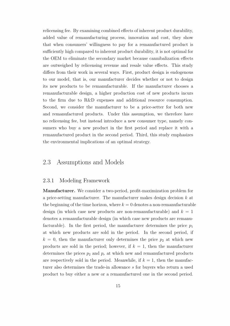
2.3 Assumptions and Models

2.3.1 Modeling Framework

Manufacturer. We consider a two-period, profit-maximization problem for

a price-setting manufacturer. The manufacturer makes design decision k at

the beginning of the time horizon, where k = 0 denotes a non-remanufacturable

design (in which case new products are non-remanufacturable) and k = 1

denotes a remanufacturable design (in which case new products are remanu-

facturable). In the first period, the manufacturer determines the price p1

at which new products are sold in the period. In the second period, if

k = 0, then the manufacturer only determines the price p2 at which new

products are sold in the period; however, if k = 1, then the manufacturer

determines the prices p2 and pr at which new and remanufactured products

are respectively sold in the period. Meanwhile, if k = 1, then the manufac-

turer also determines the trade-in allowance s for buyers who return a used

product to buy either a new or a remanufactured one in the second period.

15

Only returned products may be remanufactured and therefore the number of

remanufactured products cannot exceed the number of products returned.

The production cost of a new product depends on the design decision k. We

assume that the unit cost to produce a new non-remanufacturable product

(defined by k = 0) and a new remanufacturable product (defined by k = 1)

is c0 and c1, respectively, where c1 ≥ c0 reflects the increased complexity

required to make a product remanufacturable (Subramanian 2012). The

unit cost to remanufacture a product is cr. We assume cr < c0 because the

per-unit remanufacturing cost can be as low as 40 to 65 percent less than

that of its new products (Ginsburg 2001).

Consumers. Willingness-to-pay (WTP) θ for a new product in the first

period is heterogeneous and uniformly distributed in the interval [0, 1], with

market size normalized to 1. We assume θ to be independent of k since

a consumer’s sustainability considerations are normally separate from the

attribute of the products themselves (Galbreth and Ghosh 2013). We call

a customer with WTP equal to θ a customer of type θ. Consistent with

Oraiopoulos et al. (2012), we make the following five assumptions: First, we

assume that the new product in the second period (if offered) is an upgraded

version of the one produced and sold in the first period, characterized by

innovation factor α, where α ≥ 1. Thus, if a consumer is willing to pay θ

for the new product in the first period, then her WTP for an upgraded new

product in the second period is α · θ. Second, we assume that a new product

in the first period depreciates with use and is characterized by durability

factor δ, where δ < 1. Thus, if the customer’s WTP is θ for a new product

in the first period, then her valuation associated with keeping the product in

the second period is δ · θ. Third, we assume that a consumer’s WTP for a

remanufactured product is less than her WTP for a new product. Thus,

if a consumer is willing to pay θ for a new product in the first period,

then her WTP for a remanufactured product in the second period is δr · θ,where remanufacturing valuation factor δr ∈ (0, 1). Fourth, we assume that

remanufacturing improves the condition of a used product. Thus, δr > δ.

Fifth, we assume that the one-period utility from an upgraded product is

less than the combined utility from a new product bought in the first period

and used for two periods. Thus, α < 1 + δ.

If a new product is remanufacturable (k = 1), then a customer purchases

at most one new unit in each period. If the customer makes a purchase in

16

the first period, then in the second period, she can either trade it in for a

new product (segment nn), trade it in for a remanufactured product if one is

available (segment nr) or keep it and thereby exit the market (segment nu). If

the customer does not make a purchase in the first period, then in the second

period, she can either buy a new product (segment on), buy a remanufactured

product if available (segment or), or remain out of the market altogether

(segment oo). Therefore, in principle, there exist six customer segments

distinguished by different customer buying strategies for the two periods.

We use “customer segment” and “customer strategy” interchangeably unless

otherwise distinguished.

Consumers are strategic in the sense that they make purchase decisions

based on the total consumer surplus associated with both periods, which we

define as the product valuations net of trade-in price s (if applicable) minus

the product prices p1, p2 and pr, as applicable. Thus, like Oraiopoulos et al.

(2012), we essentially assume that consumers know the trade-in program

as well as the price list for both periods before making decisions. Note

that consumers who otherwise would have a negative consumer surplus do

not make any purchases (segment oo). We denote segment size by d with

a subscript to refer to the segment, e.g., dnn denotes the size of customer

segment nn. Therefore, we have dnn + dnr + dnu + don + dor + doo = 1.

For parsimony, we assume that used products cannot be directly traded

between customers. If a new product is non-remanufacturable (k = 0),

then the market segmentation is analogous except that k = 0 means that

dnr = dor = 0 by definition. Table 2.1 summarizes the total consumer surplus

associated with each strategy for a customer of type θ, given p1, p2, pr and

s, as applicable for a given k. In Table 2.1, note that because α > δr

by assumption, a consumer belonging to segment nn has a higher WTP θ

for a new product than a consumer belonging to segment nr (denoted by

Θnn ≻ Θnr). More broadly, by virtue of the five WTP assumptions itemized

at the beginning of this subsection, we have Θnn ≻ Θnr ≻ Θnu ≻ Θon ≻ Θor.

Thus, the customer segmentation orderings implicit in Table 2.1 (and in

Table 2.2 later) hold true for any given pricing scheme p1, p2, pr and s.

Profit-maximization Problem: Let Πk be the manufacturer’s total

profit over the two periods, given design decision k. If new products are

designed to be non-remanufacturable (k = 0), then the manufacturer’s prob-

17

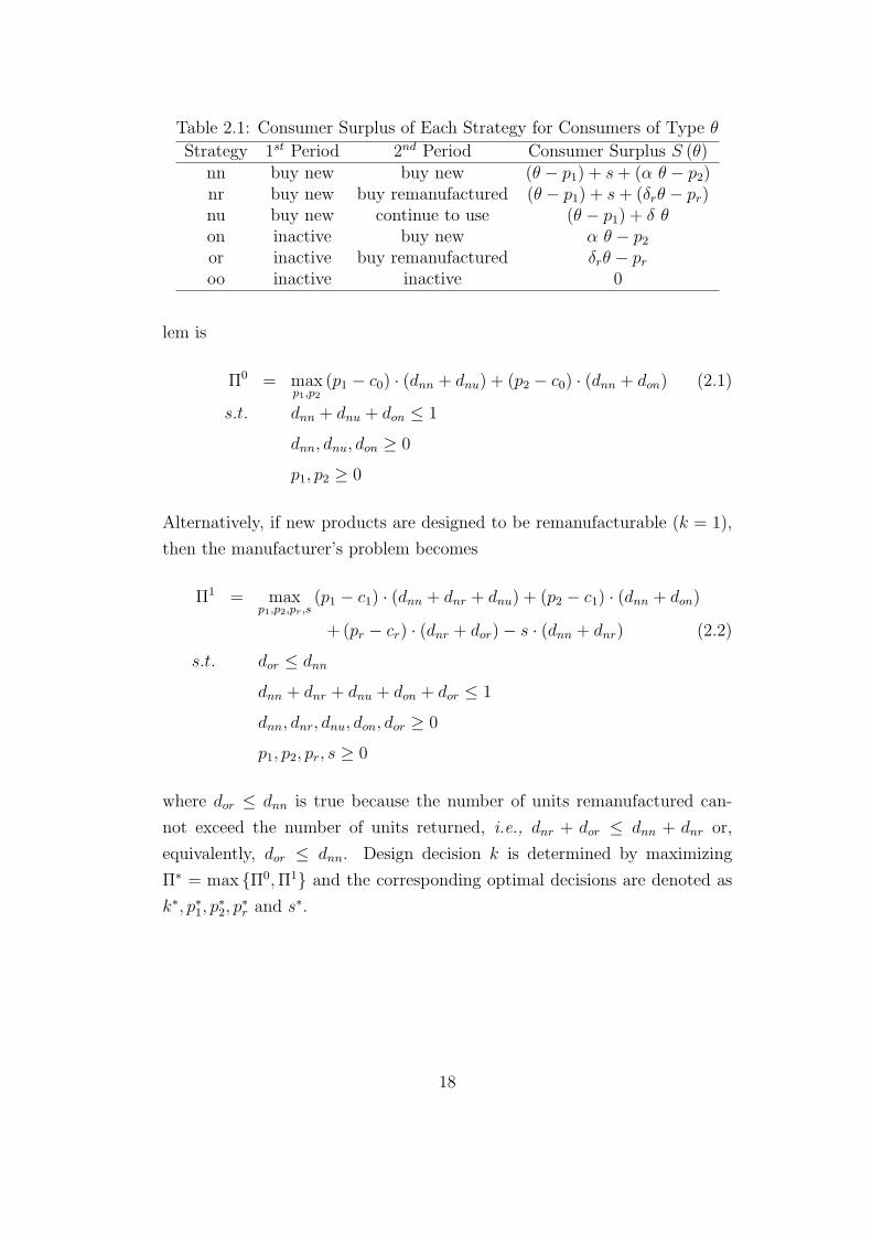
Table 2.1: Consumer Surplus of Each Strategy for Consumers of Type θ

Strategy 1st Period 2nd Period Consumer Surplus S (θ)nn buy new buy new (θ − p1) + s+ (α θ − p2)nr buy new buy remanufactured (θ − p1) + s+ (δrθ − pr)nu buy new continue to use (θ − p1) + δ θon inactive buy new α θ − p2or inactive buy remanufactured δrθ − proo inactive inactive 0

lem is

Π0 = maxp1,p2

(p1 − c0) · (dnn + dnu) + (p2 − c0) · (dnn + don) (2.1)

s.t. dnn + dnu + don ≤ 1

dnn, dnu, don ≥ 0

p1, p2 ≥ 0

Alternatively, if new products are designed to be remanufacturable (k = 1),

then the manufacturer’s problem becomes

Π1 = maxp1,p2,pr,s

(p1 − c1) · (dnn + dnr + dnu) + (p2 − c1) · (dnn + don)

+ (pr − cr) · (dnr + dor)− s · (dnn + dnr) (2.2)

s.t. dor ≤ dnn

dnn + dnr + dnu + don + dor ≤ 1

dnn, dnr, dnu, don, dor ≥ 0

p1, p2, pr, s ≥ 0

where dor ≤ dnn is true because the number of units remanufactured can-

not exceed the number of units returned, i.e., dnr + dor ≤ dnn + dnr or,

equivalently, dor ≤ dnn. Design decision k is determined by maximizing

Π∗ = max Π0,Π1 and the corresponding optimal decisions are denoted as

k∗, p∗1, p∗2, p

∗r and s∗.

18

2.3.2 Solution Procedure

For any given product design, we use Table 2.1 to obtain the indifference

point θ between any pair of customer segments such that a customer of

type θ is indifferent between two strategies, and under the assumption that

0 < δ < δr < 1 < α < 1 + δ, we produce Table 2.2 accordingly. In Table

2.2, customers with WTP above the indifference point θ in a cell belong to

the customer segment of the corresponding row and those with WTP below

the indifference point θ belong to the customer segment of the corresponding

column. If the indifference point θ is greater than or equal to one (less than

or equal to zero), then it means that all customers prefer the strategy of

the corresponding column (row) to the strategy of the corresponding row

(column). We therefore can derive the size of each segment by comparing

these indifference points. For example, if products are remanufacturable,

then Table 2.2(a) establishes that, for a customer to choose strategy nr, her

WTP θ must satisfy

θ ∈max

pr − s

δr − δ,p1 − p2 + pr − s

1 + δr − α, p1 − s,

p1 + pr − s

1 + δr, 0

,

min

p2 − prα− δr

, 1

(2.3)

In other words, if k = 1, then for a customer to choose strategy nr, that strat-

egy must yield a higher consumer surplus than would strategies nu, on, or, oo.

As per the “nr” row of Table 2.2(a), this would be true if

θ ≥ max

pr − s

δr − δ,p1 − p2 + pr − s

1 + δr − α, p1 − s,

p1 + pr − s

1 + δr

. (2.4)

Meanwhile, for the customer to choose strategy nr, that strategy also must

yield a higher consumer surplus than would strategy nn, which would be true

if θ ≤ p2−prα−δr

, as per the “nr” column of Table 2.2(a). Note that θ ∈ [0, 1],

thus Equation 2.3 follows. Given (2.3), then, the size of customer segment

nr is

dnr = max

0,min

p2 − prα− δr

, 1

−

max

pr − s

δr − δ,p1 − p2 + pr − s

1 + δr − α, p1 − s,

p1 + pr − s

1 + δr, 0

(2.5)

19

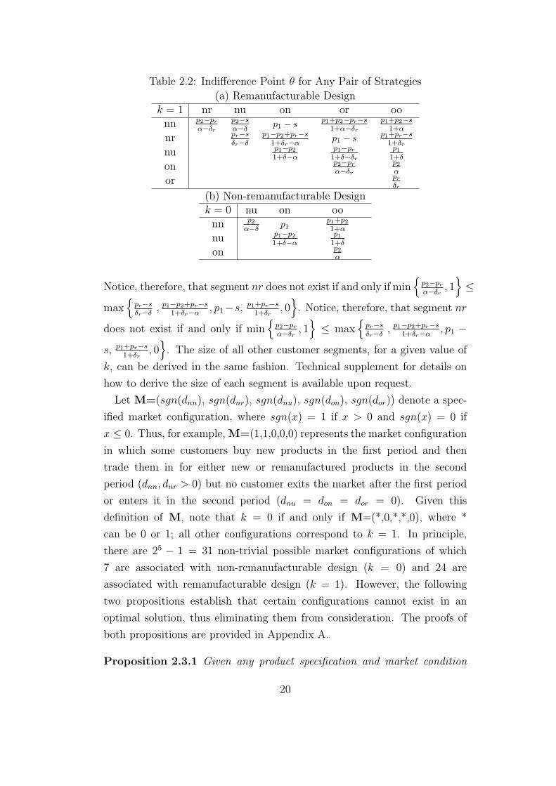
Table 2.2: Indifference Point θ for Any Pair of Strategies

(a) Remanufacturable Designk = 1 nr nu on or oonn p2−pr

α−δr

p2−sα−δ

p1 − sp1+p2−pr−s

1+α−δr

p1+p2−s1+α

nr pr−sδr−δ

p1−p2+pr−s1+δr−α

p1 − sp1+pr−s1+δr

nu p1−p21+δ−α

p1−pr1+δ−δr

p11+δ

on p2−prα−δr

p2α

or prδr

(b) Non-remanufacturable Designk = 0 nu on oonn p2

α−δp1

p1+p21+α

nu p1−p21+δ−α

p11+δ

on p2α

Notice, therefore, that segment nr does not exist if and only if min

p2−prα−δr

, 1≤

max

pr−sδr−δ

, p1−p2+pr−s1+δr−α

, p1−s, p1+pr−s1+δr

, 0. Notice, therefore, that segment nr

does not exist if and only if min

p2−prα−δr

, 1

≤ max

pr−sδr−δ

, p1−p2+pr−s1+δr−α

, p1 −

s, p1+pr−s1+δr

, 0. The size of all other customer segments, for a given value of

k, can be derived in the same fashion. Technical supplement for details on

how to derive the size of each segment is available upon request.

Let M=(sgn(dnn), sgn(dnr), sgn(dnu), sgn(don), sgn(dor)) denote a spec-

ified market configuration, where sgn(x) = 1 if x > 0 and sgn(x) = 0 if

x ≤ 0. Thus, for example,M=(1,1,0,0,0) represents the market configuration

in which some customers buy new products in the first period and then

trade them in for either new or remanufactured products in the second

period (dnn, dnr > 0) but no customer exits the market after the first period

or enters it in the second period (dnu = don = dor = 0). Given this

definition of M, note that k = 0 if and only if M=(*,0,*,*,0), where *

can be 0 or 1; all other configurations correspond to k = 1. In principle,

there are 25 − 1 = 31 non-trivial possible market configurations of which

7 are associated with non-remanufacturable design (k = 0) and 24 are

associated with remanufacturable design (k = 1). However, the following

two propositions establish that certain configurations cannot exist in an

optimal solution, thus eliminating them from consideration. The proofs of

both propositions are provided in Appendix A.

Proposition 2.3.1 Given any product specification and market condition

20

(c0, c1, cr, α, δ and δr), the following are true:

(i) dor > 0 ⇒ dnn > 0, i.e., M=(0,*,*,*,1) does not exist, where * can be

0 or 1.

(ii) dnr > 0 ⇒ don = 0 and don > 0 ⇒ dnr = 0, i.e., M=(*,1,*,1,*) does

not exist, where * can be 0 or 1.

(iii) dnr = dnu = don = dor = 0 ⇒ dnn = 0, i.e., M=(1,0,0,0,0) does not

exist.

Intuitively, Proposition 2.3.1(i) is a result of the fact that the manufacturer

cannot remanufacture more products than are returned (dor ≤ dnn). Accord-

ing to the proof of Proposition 2.3.1(ii), the existence of segment on effectively

requires that p1− s (the price of new products in the first period net of their

trade-in value) must be relatively large while p2 − pr, the price difference of

new and remanufactured products in the second period, must be relatively

small, which in turns makes it irrational to buy a new product in the first

period and then trade it in for a remanufactured product because p1− s+ pr

is relatively large. Similarly, for segment nr to exist, p1−s must be relatively

small and p2 − pr must be relatively large, in which case there would be no

demand for new products in the second period because p2 is relatively large.

The proof of Proposition 2.3.1(iii) indicates that if products are designed to

be non-remanufacturable (k = 0) and if there exist customers who makes

purchases in both periods, then it means that p1 must be sufficiently low

so as to entice some other customers to purchase new products in the first

period without then purchasing anew in the second period, thus rendering

it impossible to sell products only to customers with the highest valuation

(segment nn).

In all, Proposition 2.3.1 eliminates 15 of the 31 theoretically possible

market configurations from consideration. Next, Proposition 2.3.2 eliminates

2 more of the remaining 16.

Proposition 2.3.2 Given any product specification and market condition

(c0, c1, cr, α, δ and δr), the following are true:

(i) It is more profitable to offer only new products in the first period (dnu >

0 and dnn = dnr = don = dor = 0) than it is to offer only new products in the

second period (don > 0 and dnn = dnr = dnu = dor = 0), i.e., M=(0,0,1,0,0)

dominates M=(0,0,0,1,0).

21

(ii) If new products are non-remanufacturable (dnr = dor = 0), then it is

more profitable to offer new products for one-time purchase only in the first

period (dnu > 0 and dnn = don = 0) than it is to offer new products for

one-time purchase in either the first period or the second period (dnu, don > 0

and dnn = 0), i.e., M=(0,0,1,0,0) dominates M=(0,0,1,1,0).

To help explain Proposition 2.3.2(i), note that the assumption 1 + δ > α

suggests that if a manufacturer offers only new products, either in the first

period or in the second period, then it should be optimal to produce and sell

the products earlier rather than later, everything else being equal. In other

words, if innovation is not sufficient, then it does the firm no benefit to delay

the introduction of a new product for a minor update. Moreover in such a

case, new products will be non-remanufacturable because the firm will not

remanufacture them. In a similar vein, Proposition 2.3.2(ii) is a byproduct

of product cannibalization in our two-period model. In particular, if the

manufacturer offers new products that are non-remanufacturable in both

periods, then some customers will prefer to buy new products in the first

period rather than to buy in the second period. Note the unit profit of

selling one new product in the second period is usually smaller than the unit

profit of selling one in the first period that can be used in both periods (see

proof for details). Consequently, the manufacturer prefers to price products

such that customers will only make purchases in the first period rather than

in the second.

Although Propositions 2.3.1 and 2.3.2 analytically eliminate all but 14

possible market configurations from the search for the optimal solutions to

(2.1) and (2.2), we find that we need to rely on a numerical search routine to

complete the optimization over the remaining feasible set of configurations.

To that end, we condition the remaining search on the different feasible

market configurations. In particular, for any given feasible market configu-

ration, we numerically solve either (2.1) or (2.2), as applicable, by applying

the Matlab build-in quadratic programming function quadprog. We then

compare the profit associated with each of the resulting solutions (one for

each feasible market configuration) to obtain the optimal solution k∗, p∗1, p∗2, p

∗r

and s∗ for any given parameter set. (See Technical Supplement for algorithm

details and justification.) Finally, we repeat this process for an exhaustive

set of input parameters to populate a comprehensive database of solutions

22

Table 2.3: Parameter Ranges for Numerical Study

Parameter Increment (I) Min Maxc0 0.1∗ I 1− Ic1 0.1∗ g0 1− Icr 0.1∗ I c0 − Iα 0.1∗ 1 2− 3× Iδ 0.1∗ α− 1 + I 1− 2× Iδr 0.1∗ δ + I 1− I

* we choose increment I = 0.005 in the cases when more than one parameters are

fixed.

to the manufacturer’s maximization problem. Table 2.3 summarizes the

specific parameter ranges used in the process for which we solved the firm’s

optimization problem. Given Table 2.3, the total number of parameter

combinations (c0, c1, cr, α, δ, δr) using an increment I = 0.1 for all parameters

is 18,720. However, in addition, we solved another approximately 36,000

instances by applying a smaller increment I = 0.005. Thus our analysis

below is based on solutions to approximately 54,000 instances of the problem.

2.4 Analysis

In this section, we compile and explore the database of optimal designs

and market configurations as well as the corresponding optimal profits and

return rates produced by the numerical optimization routine applied to the

comprehensive set of problem instances as described above. To set the stage,

we note first that, although 14 possible market configurations survive the

elimination procedure implied by Propositions 2.3.1 and 2.3.2, we find that

seven of those that remain never appear in our database of optimal solutions.

Thus, we find that, of the 31 non-trivial possible market configurations that

can exist in principle, only eight remain as potentially optimal for a given set

of problem parameters taken from Table 2.3. We label these 8 configurations

as M1 through M8, and we provide each of their specifications in Table 2.4.

From Table 2.4, note that M1, M2 and M3 each have dnr = dor = 0, which

implies that k∗ = 0 when any one of these configurations is optimal; and M4

to M8 each of have either or both dnr > 0 or dor > 0, which implies that

k∗ = 1 when any one of these configurations is optimal.

23

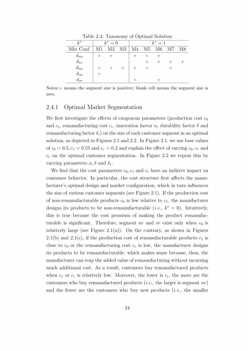
Table 2.4: Taxonomy of Optimal Solution

k∗ k∗ = 0 k∗ = 1Mkt Conf. M1 M2 M3 M4 M5 M6 M7 M8

dnn + + + + +

dnr + + + +

dnu + + + + + +

don +

dor + +

Notes:+ means the segment size is positive; blank cell means the segment size is

zero.

2.4.1 Optimal Market Segmentation

We first investigate the effects of exogenous parameters (production cost c0

and c1, remanufacturing cost cr, innovation factor α, durability factor δ and

remanufacturing factor δr) on the size of each customer segment in an optimal

solution, as depicted in Figures 2.1 and 2.2. In Figure 2.1, we use base values

of c0 = 0.5, c1 = 0.55 and cr = 0.2 and explain the effect of varying c0, c1 and

cr on the optimal customer segmentation. In Figure 2.2 we repeat this by

varying parameters α, δ and δr.

We find that the cost parameters c0, c1 and cr have an indirect impact on

consumer behavior. In particular, the cost structure first affects the manu-

facturer’s optimal design and market configuration, which in turn influences

the size of various customer segments (see Figure 2.1). If the production cost

of non-remanufacturable products c0 is low relative to c1, the manufacturer

designs its products to be non-remanufacturable (i.e., k∗ = 0). Intuitively,

this is true because the cost premium of making the product remanufac-

turable is significant. Therefore, segment nr and or exist only when c0 is

relatively large (see Figure 2.1(a)). On the contrary, as shown in Figures

2.1(b) and 2.1(c), if the production cost of remanufacturable products c1 is

close to c0 or the remanufacturing cost cr is low, the manufacturer designs

its products to be remanufacturable, which makes sense because, then, the

manufacturer can reap the added value of remanufacturing without incurring

much additional cost. As a result, customers buy remanufactured products

when c1 or cr is relatively low. Moreover, the lower is cr, the more are the

customers who buy remanufactured products (i.e., the larger is segment nr)

and the fewer are the customers who buy new products (i.e., the smaller

24

oo

nu

nn

oo

nu

nn

oo

or

nr

nn

oo

or

nr

nn

c00.40 0.45 0.50 0.55HaL c1=0.55, cr=0.2

0.0

0.2

0.4

0.6

0.8

1.0

oo

or

nr

nn

oo

or

nr

nn

oo

nu

nn

oo

nu

nn

c10.50 0.55 0.60 0.65HbL c0=0.5, cr=0.2

0.0

0.2

0.4

0.6

0.8

1.0

oo

or

nr

nn

oo

or

nr

nn

oo

or

nr

nn

oo

nu

nn

cr0.10 0.15 0.20 0.25HcL c0=0.5, c1=0.55

0.0

0.2

0.4

0.6

0.8

1.0

Figure 2.1: Customer Segments (α = 1.25, δ = 0.4 and δr = 0.8)

is segment nn). Intuitively, a lower cr allows the manufacturer to lower the

price of remanufactured products. Interestingly, however, the size of segment

or also increases as cr increases (see Figure 2.1(c)). This is because some

customers who otherwise would choose strategy nr when cr is small switch

to strategy or when cr is large, which results in a higher pr and a lower

s. Nevertheless, as a whole, the overall sale of remanufactured products

reduces as cr increases (see Figure 2.1(c)). In a similar vein, the overall

sale of remanufactured products initially increases as c1 increases because

some customers who otherwise would choose strategy nn when c1 is small

switch to purchase remanufactured products in the second period when c1

(and, correspondingly p1 and p2) grow larger. Eventually, however, if c1 is

sufficiently large, then the manufacturer’s optimal design becomes k∗ = 0

in which case segments nr and or necessarily disappear altogether because

remanufactured products are not available.

Looking next at Figure 2.2, we find that when innovation factor α increases,

more customers buy new products in both periods (i.e., dnn increases), but

fewer customers buy remanufactured products (i.e., dnr + dor decreases).

This is because customers are willing to pay more for upgraded products

when α is larger. Interestingly, however, we find that although the overall

demand for remanufactured products (dnr + dor) decreases in α, the size of

segment or increases in α. Intuitively, this happens because, as α increases,

the manufacturer can provide less incentive to attract previous buyers (i.e.,

provide smaller s), which enables it to reduce its price for remanufactured

products (i.e., reduce pr) to expand segment or. Similarly, a larger durability

factor δ means that more customers find it optimal to continue using the old

25

oo

or

nr

nn

oo

or

nr

nn

oo

or

nr

nn

oo

or

nr

nn

Α

1.10 1.15 1.20 1.25HaL ∆=0.4, ∆r=0.8

0.0

0.2

0.4

0.6

0.8

1.0

oo

or

nr

nn

oo

or

nu

nn

oo

nu

oo

nu

∆

0.40 0.50 0.60 0.70HbL Α=1.25, ∆r=0.8

0.0

0.2

0.4

0.6

0.8

1.0

oo

nu

nn

oo

or

nr

nn

oo

or

nr

nn

oo

or

nr

nn

∆r0.75 0.80 0.85 0.90HcL Α=1.25, ∆=0.4

0.0

0.2

0.4

0.6

0.8

1.0

Figure 2.2: Customer Segments (c0 = 0.5, c1 = 0.55 and cr = 0.2)

Table 2.5: Characterization of the Optimal Solution (c0 = 0.5, cr = 0.2,α = 1.25)

Mkt Conf. M1 M2 M3 M4* M5* M6* M7* M8*

Fig 2.3(a) c1 = 0.50 (%) 0.0 0.0 7.0 64.4 0.0 27.2 1.4 0.0 100%

Fig 2.3(b) c1 = 0.55 (%) 0.0 34.0 40.1 2.1 0.0 23.5 0.3 0.0 100%

Fig 2.3(c) c1 = 0.60 (%) 0.0 45.9 45.4 0.0 0.0 8.7 0.0 0.0 100%

Notes: * indicates market configurations corresponding to k∗ = 1. Each row

represents the percentage of cases (varying δ and δr) for which the given market

configuration constitutes the optimal solution for given c1.

product in the second period (i.e., dnu increases), while fewer customers buy

upgraded or remanufactured products (i.e., dnn, dnr and dor all decrease). In

general, δr produces the mirror effect that cr produces as shown in Figure

2.2(c). In particular, as δr increases, while dnr increases and dnu decreases;

and the progressions of dor and dnn are monotonically decreasing as long as

k∗ = 1.

2.4.2 Optimal Product Design

As seen from Figure 2.2, the manufacturer tends to design a non-remanufacturable

product (k∗ = 0) when product durability δ is relatively large or reman-

ufacturing valuation factor δr is relatively small. We next examine more

closely the effect of these two parameters on the optimal product design.

Toward that end, Figure 2.3 illustrates the optimal product design and

market configurations as functions of (δ, δr) space for various values of c1,

given that c0 = 0.5, cr = 0.2 and α = 1.25. Each solid curve in the figure

represents the threshold above which k∗ = 1.

26

0.25 0.5 0.75 10.25

0.5

0.75

1

(a) c1=0.50

δ

δr

M6

M4

M3M7

0.25 0.5 0.75 10.25

0.5

0.75

1

(b) c1=0.55

δ

δr

M6

M7

M4

M3

M2

0.25 0.5 0.75 10.25

0.5

0.75

1

(c) c1=0.60

δ

δr

M6

M2

M3

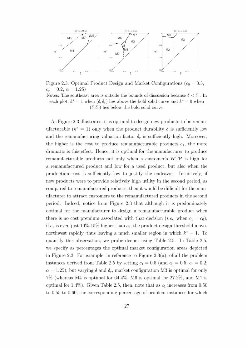
Figure 2.3: Optimal Product Design and Market Configurations (c0 = 0.5,cr = 0.2, α = 1.25)Notes: The southeast area is outside the bounds of discussion because δ < δr. In

each plot, k∗ = 1 when (δ, δr) lies above the bold solid curve and k∗ = 0 when

(δ, δr) lies below the bold solid curve.

As Figure 2.3 illustrates, it is optimal to design new products to be reman-

ufacturable (k∗ = 1) only when the product durability δ is sufficiently low

and the remanufacturing valuation factor δr is sufficiently high. Moreover,

the higher is the cost to produce remanufacturable products c1, the more

dramatic is this effect. Hence, it is optimal for the manufacturer to produce

remanufacturable products not only when a customer’s WTP is high for

a remanufactured product and low for a used product, but also when the

production cost is sufficiently low to justify the endeavor. Intuitively, if

new products were to provide relatively high utility in the second period, as

compared to remanufactured products, then it would be difficult for the man-

ufacturer to attract customers to the remanufactured products in the second

period. Indeed, notice from Figure 2.3 that although it is predominately

optimal for the manufacturer to design a remanufacturable product when

there is no cost premium associated with that decision (i.e., when c1 = c0),

if c1 is even just 10%-15% higher than c0, the product design threshold moves

northwest rapidly, thus leaving a much smaller region in which k∗ = 1. To

quantify this observation, we probe deeper using Table 2.5. In Table 2.5,

we specify as percentages the optimal market configuration areas depicted

in Figure 2.3. For example, in reference to Figure 2.3(a), of all the problem

instances derived from Table 2.5 by setting c1 = 0.5 (and c0 = 0.5, cr = 0.2,

α = 1.25), but varying δ and δr, market configuration M3 is optimal for only

7% (whereas M4 is optimal for 64.4%, M6 is optimal for 27.2%, and M7 is

optimal for 1.4%). Given Table 2.5, then, note that as c1 increases from 0.50

to 0.55 to 0.60, the corresponding percentage of problem instances for which

27

0.3 0.35 0.4 0.45 0.5 0.55 0.6 0.65 0.7 0.75

0.25

0.3

0.35

0.4

0.45

0.5

0.55

0.6

δ

c1

(a) cr=0.2, α=1.25, δ

r=0.8

c0=0.3

c0=0.4

c0=0.5

0.5 0.6 0.7 0.8 0.90.25

0.3

0.35

0.4

0.45

0.5

0.55

0.6

0.65

0.7

δr

c1

(b) cr=0.2, α=1.25, δ=0.4

c0=0.3

c0=0.4

c0=0.5

1 1.05 1.1 1.15 1.2 1.25 1.3 1.35

0.3

0.35

0.4

0.45

0.5

0.55

0.6

α

c1

(c) cr=0.2, δ=0.4, δ

r=0.8

c0=0.3

c0=0.4

c0=0.5

0.05 0.1 0.15 0.2 0.25 0.3 0.35 0.4 0.45

0.35

0.4

0.45

0.5

0.55

0.6

0.65

0.7

cr

c1

(d) α=1.25, δ=0.4, δr=0.8

c0=0.3

c0=0.4

c0=0.5

Figure 2.4: Maximum Threshold of c1 for a Remanufacturable Design

k∗ = 1 (M4-M8) decreases rapidly, but at a decreasing rate, from 93% to

25.9% to 8.7%.

To further relate the above observation to optimal design, we next find

the upper bound of c1 beyond which the manufacturer chooses not to design

a remanufacturable product. Figure 2.4 depicts this threshold as a function

of various problem parameters. In Figure 2.4, values of c1 below a given

threshold function correspond to k∗ = 1 and values above the threshold

function correspond to k∗ = 0. Intuitively, when customers are willing to

pay more for a remanufactured product (i.e., the larger is δr) or when the

remanufacturing cost is lower (i.e., the smaller is cr), the manufacturer will

continue to design and produce remanufacturable products at higher costs

(i.e., at higher values of c1). However, it is interesting to note from Figure

2.4(a) that the remanufacturable design threshold of c1 is not a monotone

function of product durability δ. To help explain this observation, it is useful

to examine the corresponding optimal market configuration when k∗ = 0.

In doing so, we find that when δ is small, the profit associated with selling

new products in both periods is higher than that associated with selling

new products only in the first period because customers who keep using

28

old products do not pay a large premium for product durability. But, if

new products are available in both periods when customers also have the

option to continue using used products, then any increase in δ essentially

intensifies product cannibalization. As a result, when δ is small and increases,

the manufacturer will choose to remanufacture even for increased costs c1

associated with doing so. In contrast, segment nu is sufficiently lucrative to

deter the manufacturer from selling new products in the second period, in

which case, any increase in δ essentially means that the manufacturer can

charge a higher price for new products and generate higher profits without

worrying about product cannibalization. Consequently, when δ is large and

increases, the manufacturer, ceteris paribus, requires a lower c1 to justify

remanufacturing.

2.4.3 Optimal Return and Remanufacturing Rates

Environmental laws such as the Waste Electrical and Electronic Equipment

(WEEE) Directive requires its member states to recollect a specific percent

of e-waste put on their markets (WEEE Directive, 2012). Nevertheless,

manufacturers recollect used products not only to comply with laws and

regulations, but also to remanufacture them to boost economic success. In

our model setting, the return rate is determined by the trade-in allowance s.

Hence, in this section, we study the implied return rate corresponding to the

manufacturer’s optimal product design and market segmentation strategy.

However, the return rate in and of itself is not necessarily the same as the

remanufacturing rate, meaning that not all returned products are necessarily

remanufactured upon their return. Hence, in this section, we also study the

resulting remanufacturing rate associated with the manufacturer’s optimal

strategy.

2.4.3.1 Return Rate

We define return rate (r) as the proportion of new products sold in the first

period that are later recollected by the manufacturer, that is,

r =dnn + dnr

dnn + dnr + dnu

29

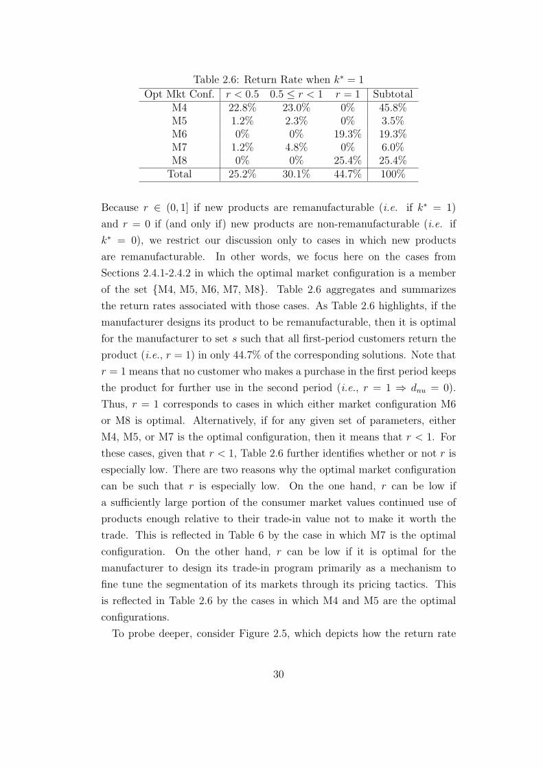
Table 2.6: Return Rate when k∗ = 1

Opt Mkt Conf. r < 0.5 0.5 ≤ r < 1 r = 1 SubtotalM4 22.8% 23.0% 0% 45.8%M5 1.2% 2.3% 0% 3.5%M6 0% 0% 19.3% 19.3%M7 1.2% 4.8% 0% 6.0%M8 0% 0% 25.4% 25.4%Total 25.2% 30.1% 44.7% 100%

Because r ∈ (0, 1] if new products are remanufacturable (i.e. if k∗ = 1)

and r = 0 if (and only if) new products are non-remanufacturable (i.e. if

k∗ = 0), we restrict our discussion only to cases in which new products

are remanufacturable. In other words, we focus here on the cases from

Sections 2.4.1-2.4.2 in which the optimal market configuration is a member

of the set M4, M5, M6, M7, M8. Table 2.6 aggregates and summarizes

the return rates associated with those cases. As Table 2.6 highlights, if the

manufacturer designs its product to be remanufacturable, then it is optimal

for the manufacturer to set s such that all first-period customers return the

product (i.e., r = 1) in only 44.7% of the corresponding solutions. Note that

r = 1 means that no customer who makes a purchase in the first period keeps

the product for further use in the second period (i.e., r = 1 ⇒ dnu = 0).

Thus, r = 1 corresponds to cases in which either market configuration M6

or M8 is optimal. Alternatively, if for any given set of parameters, either

M4, M5, or M7 is the optimal configuration, then it means that r < 1. For

these cases, given that r < 1, Table 2.6 further identifies whether or not r is

especially low. There are two reasons why the optimal market configuration

can be such that r is especially low. On the one hand, r can be low if

a sufficiently large portion of the consumer market values continued use of

products enough relative to their trade-in value not to make it worth the

trade. This is reflected in Table 6 by the case in which M7 is the optimal

configuration. On the other hand, r can be low if it is optimal for the

manufacturer to design its trade-in program primarily as a mechanism to

fine tune the segmentation of its markets through its pricing tactics. This

is reflected in Table 2.6 by the cases in which M4 and M5 are the optimal

configurations.

To probe deeper, consider Figure 2.5, which depicts how the return rate

30

r, as well as and the associated trade-in price s required to induce that

return rate, change as selected parameters change. As Figure 2.5(a) shows,

both r and s generally increase as δr increases. This basically reflects the

fact that, the higher is δr, the more profit the manufacturer can gain from

remanufactured products and, thus, the more incentive the manufacturer has

to increase its trade-in price so that it can recollect enough used products

to sufficiently endow its remanufacturing operation. However, as δ increases,

r actually decreases despite increases in s. The intuition is as follows. The

higher is δ, the more a consumer values ownership of a previous purchase

relative to a replacement purchase, regardless of whether that replacement

would be new or remanufactured. Hence, the higher is δ, the higher the

trade-in price needs to be to stimulate any returns, but, at the same time,

the less willing are consumers to respond to that incentive. Conversely,

Figure 2.5(b) indicates that r generally increases, while s generally decreases,

with increases in α. Intuitively, if α is relatively large, then it means that

consumers are more willing to buy new products in the second period, thus

they are willing to trade-in previous purchases without deterrence from a

relatively lower s. Nevertheless, as Figure 2.5(c) illustrates, r and s both grow

comparatively larger when a high c0 is coupled with a small cr. Intuitively, in

such a scenario, the potential benefit of cost savings (i.e., c0 − cr) dominates

the potential negative effect of product cannibalization; hence, it is profitable

to recollect more used products for remanufacturing and that requires a

relatively larger s to fuel the process.

2.4.3.2 Remanufacturing Rate

Although the return rate r effectively reveals how much incentive a manufac-

turer provides consumers through its trade-in price s to return used products

for replacement purchases, not all recollected products will necessarily be

remanufactured, particularly if the manufacturer uses its trade-in program

simply as a way to more finely segment its market through pricing tactics.

Therefore, it is important also to examine the remanufacturing rate (rm),

which we define as the proportion of returned products that are actually

remanufactured. That is,

rm =dnr + dordnn + dnr

31

Figure 2.5: Return Rate and Minimum s

Notes: Pattern areas represent when it is optimal for the manufacturer to design

and produce remanufactured products.

By definition, rm ∈ (0, 1] and is only valid if k∗ = 1. If rm = 1, then it

means that the manufacturer recollects used products solely for the purpose

of remanufacturing rather than for the purpose of fine-tuning its market

segmentation. According to Table 2.7, we find that rm = 1 in more than half

of the optimal solutions corresponding to k∗ = 1 (58.4%). On the contrary,

we also find that rm < 0.5 in more than one third of optimal solutions

corresponding to k∗ = 1 (37.5%). It is these cases, in particular, that suggest

that it very well could be in the manufacturer’s interest to use its trade-in

program not for the purpose of endowing its remanufacturing process, per se,

but rather for the purpose of stimulating repurchases of new products while

reducing the cannibalization of those repurchases. As Table 2.7 illustrates,

this occurs when M4 or M5 is the optimal market configuration. Indeed,

according to Table 2.7, M5 is especially likely to be associated with a low

rm. Intuitively, this is true because M5 is optimal when α is relatively small,

which signifies that remanufactured products intensively cannibalize the sale

of new products, when c1 is close to c0, which signifies that the cost of offering

a trade-in program is low, and when cr is large, which signifies that the cost

of producing remanufactured products is high.

Given Table 2.7, Figure 2.6 further illustrates how rm changes as se-

lected parameters change. Like the return rate r, and for analogous reasons,

32

Table 2.7: Remanufacturing Rate when k∗ = 1

Opt Mkt Conf. rm < 0.5 0.5 ≤ rm < 1 rm = 1 SubtotalM4 32.9% 2.1% 10.8% 45.8%M5 3.5% 0.0% 0% 3.5%M6 1.1% 2.0% 16.2% 19.3%M7 0% 0% 6.0% 6.0%M8 0% 0% 25.4% 25.4%Total 37.5% 4.1% 58.4% 100%

the remanufacturing rate rm increases in δr and decreases in δ (see Figure

2.6(a)). However, unlike the return rate r, the remanufacturing rate rm

generally decreases in α (see Figure 2.6(b)). This is true because, when

α is relatively large, it means that customers prefer upgraded products to

remanufactured products, thus a remanufacturable product design primarily

serves the purpose of more finely segmenting the market, and this drives rm

down. Nevertheless, Figure 2.6(b) also suggests that rm generally increases

as c1 increases. This is true because, as c1 increases, it becomes more

costly for the manufacturer to produce remanufacturable products. As a

result, the manufacturer will choose a remanufacturable product design only

if it is profitable to sell remanufactured products, which drives rm up. By

comparing Figure 2.6(c) to 2.5(c), we find that although the manufacturer

recollects more than half of the products it sells in the first period when

c0 and cr are both high (Figure 2.5 (c)), the manufacturer actually reman-

ufactures less than 10% of those recollected units (Figure 2.6 (c)). This

is because when the cost of producing non-remanufacturable products c0 is

high, switching to a remanufacturable design does not significantly increase

the associated production cost (i.e., c1 − c0 is relatively small) but it does

enable the manufacturer to extract additional value by further segmenting its

market through its trade-in program. However, because of the relatively high

remanufacturing cost cr, it is not profitable to remanufacture the recollected

products. As a result, although r is sufficiently large, rm is nevertheless close

to zero.

33

Figure 2.6: Remanufacturing RateNotes: Pattern areas represent when it is optimal for the manufacturer to design

and produce remanufactured products.

2.5 Environmental Impact

Among other reasons, return rates in general, and remanufacturing rates

in particular, are important because they serve as useful metrics that help

gauge how a manufacturer’s product design affects its environmental impact.

However, metrics for assessing environmental impact have yet to be stan-

dardized. For example, whereas the EPA focuses on establishing standards

that essentially limit the emissions released through per-unit consumption

(United States Environmental Protection Agency 2012), the EU Emissions

Trading System (EU ETS) focuses on establishing standards that essentially

limit the emissions released during production (EU ETS 2012). Moreover,

regardless of laws and regulations, manufacturers sometimes adopt their

own environmental performance metrics for internal control. For example,

one such metric, adopted by Apple Inc., is emissions per revenue (Apple

2013). Accordingly, in this section, we assess the environmental impact of

the manufacturer’s optimal product design and market segmentation strategy

from Section 2.4 by considering its performance across several commonly

applied metrics introduced by government or industry. Toward that end, we

compare the manufacturer’s optimal product design k∗ ∈ 0, 1 from Section

2.4 to the environmentally friendly design kef ∈ 0, 1 associated with a

given environmental impact metric, where the definition of kef depends on

the specific metric ef under consideration. For example, if ef(k) denotes

the specific metric under consideration such that the lower is ef(k) the more

environmentally friendly is the product design, then we say that kef = 1 if

and only if ef (k = 1) ≤ ef (k = 0). For each environmental impact measure

ef that we consider in this section, we compare k∗ to kef for each of the 18,720

34

problem instances defined by Table 2.3 when using the increment I = 0.1;

and for any given problem instance and specified value of k, we assume that

the manufacturer chooses the optimal market segmentation conditioned on

that value of k.

Within this context, we compare k∗ and kef across the comprehensive

set of problem instances to assess the extent to which a manufacturer’s

remanufacturable product design (whether optimal or not) will be environ-

mentally friendly (i.e., kef = 1), on the one hand, and the extent to which a

manufacturer’s optimal product design is consistent with the environmentally

friendly design (i.e., k∗ = kef ), on the other hand, for different definitions

of environmental impact metric ef . Moreover, we compare and contrast

these assessments across the various definitions of ef to ascertain the virtues

associated with adopting or imposing any particular metric over another. We

begin by establishing the notion of total emissions within the context of our

model.

2.5.1 Emissions

Given that one of the most acknowledged environmental impact metrics is

total emissions, we model emissions in a similar spirit as Agrawal et al. (2012),

Atasu and Souza (2013) and Gu et al. (2012). In particular, we assume

that the emissions of producing one unit of new product is ep, the emissions

associated with remanufacturing (if applicable) and with consuming a unit of

product is er and ec, respectively, and the emissions associated with disposing

the remains of a unit of product is ed. Given this construct and the sizes of all

customer segments (dnn, dnr, dnu, don and dor), the total emissions of produc-

ing new products is ep (2 · dnn + dnr + dnu + don) and the total emissions of

producing remanufactured products is er (dnr + dor). Correspondingly, the

total emissions associated with the consumption of those new and reman-

ufactured products is ec (2 · dnn + 2 · dnr + dnu + don + dor). Note that all

products originally produced are eventually disposed, however the sources

of disposal are twofold: on the one hand, consumers dispose the products in

their possession at the end of the second period (dnn+dnr+dnu+don+dor), but

they do not dispose any products at the end of the first period because, at that

time, they either keep the product for another period of use or they return

35

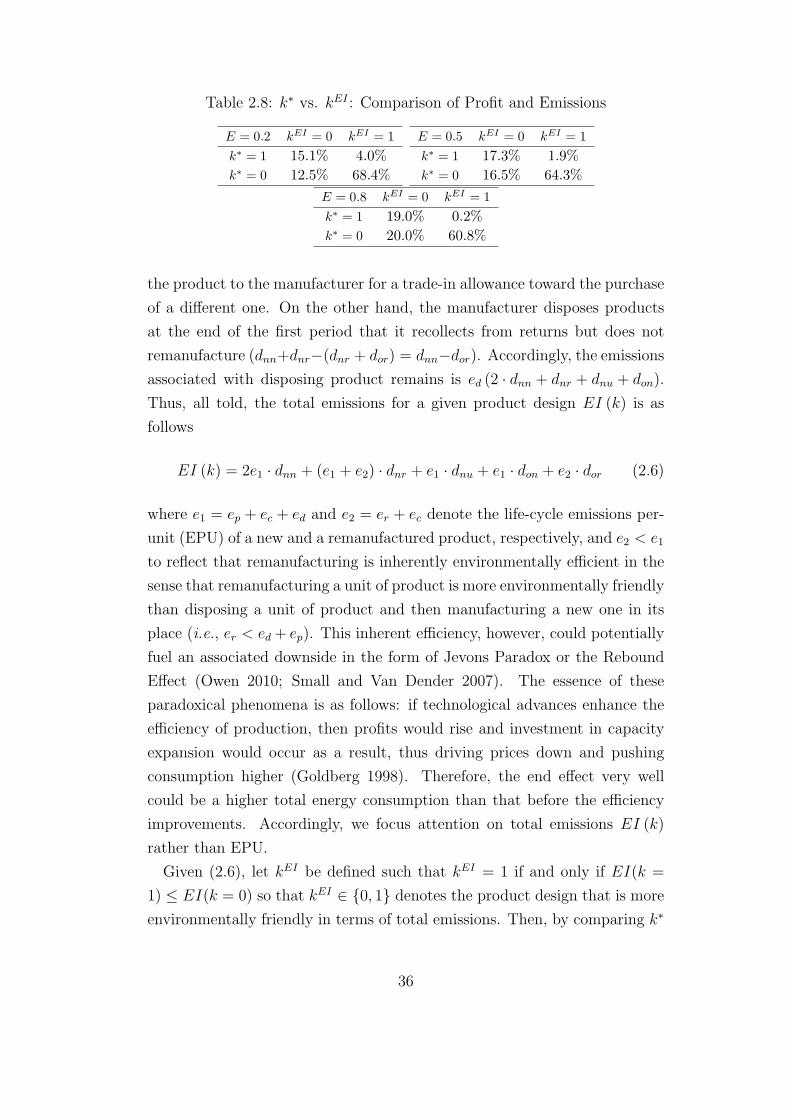
Table 2.8: k∗ vs. kEI : Comparison of Profit and Emissions

E = 0.2 kEI = 0 kEI = 1

k∗ = 1 15.1% 4.0%

k∗ = 0 12.5% 68.4%

E = 0.5 kEI = 0 kEI = 1

k∗ = 1 17.3% 1.9%

k∗ = 0 16.5% 64.3%

E = 0.8 kEI = 0 kEI = 1

k∗ = 1 19.0% 0.2%

k∗ = 0 20.0% 60.8%

the product to the manufacturer for a trade-in allowance toward the purchase

of a different one. On the other hand, the manufacturer disposes products

at the end of the first period that it recollects from returns but does not

remanufacture (dnn+dnr−(dnr + dor) = dnn−dor). Accordingly, the emissions

associated with disposing product remains is ed (2 · dnn + dnr + dnu + don).

Thus, all told, the total emissions for a given product design EI (k) is as

follows

EI (k) = 2e1 · dnn + (e1 + e2) · dnr + e1 · dnu + e1 · don + e2 · dor (2.6)

where e1 = ep + ec + ed and e2 = er + ec denote the life-cycle emissions per-

unit (EPU) of a new and a remanufactured product, respectively, and e2 < e1

to reflect that remanufacturing is inherently environmentally efficient in the

sense that remanufacturing a unit of product is more environmentally friendly

than disposing a unit of product and then manufacturing a new one in its

place (i.e., er < ed + ep). This inherent efficiency, however, could potentially

fuel an associated downside in the form of Jevons Paradox or the Rebound

Effect (Owen 2010; Small and Van Dender 2007). The essence of these

paradoxical phenomena is as follows: if technological advances enhance the

efficiency of production, then profits would rise and investment in capacity

expansion would occur as a result, thus driving prices down and pushing

consumption higher (Goldberg 1998). Therefore, the end effect very well

could be a higher total energy consumption than that before the efficiency

improvements. Accordingly, we focus attention on total emissions EI (k)

rather than EPU.

Given (2.6), let kEI be defined such that kEI = 1 if and only if EI(k =

1) ≤ EI(k = 0) so that kEI ∈ 0, 1 denotes the product design that is more

environmentally friendly in terms of total emissions. Then, by comparing k∗

36

and kEI for each of the 18,720 problem instances from Table 2.3, we obtain

Table 2.8, where each subtable corresponds to a different value of E := e2e1.

According to Table 2.8, for example, if E = 0.5, then it means that although

a remanufacturable product design is environmentally friendly (kEI = 1)

in 66.20% of the 18,720 problem instances considered, that design is also

optimal (k∗ = kEI = 1) in only 1.86% of the 18,720 instances.

We make several observations from Table 2.8. First, although a remanu-

facturable product design generally results in lower emissions as compared

to a non-remanufacturable product design (in the sense that kEI = 1 in

approximately 60%-70% of the problem instances), a remanufacturable prod-

uct design in and of itself is not necessarily synonymous with environmental

friendliness (in the sense that kEI = 0 in approximately 30%-40% of the

problem instances). Second, by and large, the optimal product design k∗

is not particularly environmentally friendly in terms of total emissions (in

the sense that k∗ = kEI in approximately 79%-83% of the the problem

instances). Third, as E increases, although the proportion of cases for which

k∗ = 0 = kEI decreases, the proportion for which k∗ = 1 = kEI increases.

Thus, all told, Table 2.8 suggests that maximizing profit typically comes at

the expense of increased total emissions. And by extrapolation, this means

that one potential drawback of a purely regulatory approach to limiting total

emissions is that it could force manufacturers to reduce its production level to

the point that it fails to meet customer needs (James 1994). For this reason,

government and industry alike often consider metrics of emissions efficiency

in lieu of total emissions, where emissions efficiency accounts for the economic

benefits generated in exchange for a unit of emissions. In other words, as

an alternative to total emissions, environmental impact can be measured byEmissions

Economic Benefits, where Economic Benefits can refer either to manufacturer

benefits (such as revenue or profit) or to societal benefits (such as consumer

surplus or social welfare). Accordingly, we next introduce four such measures

before proceeding to assess their relative significance in Section 2.5.2.

Emissions Per Revenue (ER). ER is an important environmental effi-

ciency metric that manufacturers not only strive to reduce, but also publish

voluntarily to communicate their environmental stewarding. See, for exam-

ple, Apple (2013), Cummins (2012) and Dell (2013). Introduced by Klassen

and McLaughlin (1996), ER gauges environmental impact by comparing a

manufacturer’s total emissions associated with the sales of its products to the

37

total revenue derived from those sales. Thus, in our context, ER (k) = EI(k)R(k)

,

where

R (k) =

p1 (dnn + dnr + dnu) + p2 (dnn + don) + pr (dnr + dor)− s (dnn + dnr)

k = 1

p1 (dnn + dnu) + p2 (dnn + don)

k = 0

(2.7)

Accordingly, let kER be defined such that kER = 1 if and only if ER (k = 1) ≤ER (k = 0) so that kER ∈ 0, 1 denotes the product design that is more

environmentally friendly in terms of the emissions per revenue efficiency ratio.

Emissions Per Profit (EP). EP is a related environmental efficiency

metric that focuses on value added in lieu of total revenue (see, for example,

Bosch 2012). Specifically, in our context, EP (k) = EI(k)Πk , where Πk is given

by (2.1) and (2.2), depending on whether k = 0 or k = 1, respectively.

Accordingly, let kEP be defined such that kEP = 1 if and only if EP (k = 1) ≤EP (k = 0) so that kEP ∈ 0, 1 denotes the product design that is more

environmentally friendly in terms of the emissions per profit efficiency ratio.

Emissions Per Consumer Surplus (EC). EC is an environmental

efficiency metric that relates emissions to the net economic benefits derived

directly from the consumption rather than the sales of the manufacturer’s

products. Given that overregulation of reuse and recycling rates has been

shown to have potentially deleterious effects on consumer surplus under

certain circumstances (Karakayali et al. 2012), EC has particular relevance

to social planners. In our context, EC (k) = EI(k)CS(k)

, where CS (k) is derived

in detail in Appendix A. Accordingly, let kEC be defined such that kEC = 1

if and only if EC (k = 1) ≤ EC (k = 0) so that kEC ∈ 0, 1 denotes the

product design that is more environmentally friendly in terms of the emissions

per consumer surplus efficiency ratio.

Emissions Per Social Welfare (EW). EW is an environmental effi-

ciency metric similar to EC except that it relates emissions to the combined

net economic benefits derived from both the consumption and the sales of the

manufacturer’s products (Orsdemir et al. 2014). In our context, EW (k) =EI(k)SW (k)

, where SW (k) is derived in detail in Appendix A. Accordingly, let kEW

be defined such that kEW = 1 if and only if EW (k = 1) ≤ EW (k = 0) so

that kEW ∈ 0, 1 denotes the product design that is more environmentally

38

Table 2.9: Environmental Efficiency Metrics

E = 0.5kEI kER kEP

0 1 0 1 0 1

k∗ = 1 17.27% 1.86% 11.56% 7.57% 9.61% 9.52%

k∗ = 0 16.53% 64.34% 17.86% 63.01% 77.06% 3.81%

Total 33.80% 66.20% 29.42% 70.58% 86.67% 13.33%

E = 0.5kEC kEW

0 1 0 1

k∗ = 1 15.68% 3.45% 16.05% 3.08%

k∗ = 0 80.27% 0.60% 24.72% 56.15%

Total 95.95% 4.05% 40.77% 59.23%

friendly in terms of the emissions per consumer surplus efficiency ratio.

2.5.2 Assessment of Environmental Impact and OptimalProduct Design

In this section, to assess the relative merits of the various environmental

efficiency metrics and their potential significance to industry and government,

we systematically compare k∗ to kef for the four ef ratios defined in Section

2.5.1 in the same spirit that we compared k∗ to kEI in Table 2.8. Toward

that end, we focus on the same 18,720 problem instances previously compiled,

and we present our results in Table 2.9 for the representative case in which

E = 0.5. Recall that, for any given metric ef (k), kef = 1 if and only if

ef (k = 1) ≤ ef (k = 0). Thus, in this section, if kef = x for metric ef , then

we say that x is the product design that is more environmentally friendly in

terms of ef .

According to Table 2.9, EP is the environmental efficiency metric that is

most consistent with a manufacturer’s optimal product design in the sense

that k∗ = kef is true for the highest percentage of problem instance (86.58%)

when ef = EP as compared to when ef ∈ ER,EC,EW. This can be

explained intuitively because EP (k) includes profit in its denominator, which

means that, everything else being equal, EP decreases as profit increases. In

this sense, environmental efficiency metric EP is particularly well aligned with

profit maximization, thus it stands to reason that k∗ = kEP would be true as

a general rule. By contrast, it is the closely related environmental efficiency

39

metric ER that is most aligned with the reduction of total emissions in the

sense that the percentage of problem instances in which kEI = 1 (66.20%) is

closer in magnitude to the percentage of problem instances in which kER = 1

(70.58%) than it is to the percentage of problem instances in which kef = 1

for ef ∈ EP,EC,EW. Indeed, the percentage of cases for which kef = 1 is

greatest for ef = ER among all environmental impact measures ef consid-

ered here. Intuitively, this makes sense because a production cost premium

is required to produce a unit of a remanufacturable product as compared to

producing a unit of a non-remanufacturable product (i.e., c1 > c0), which in

turn means that k = 1 typically corresponds to a higher associated per-unit

revenue as compared to k = 0, everything else being equal. Correspondingly,

ER(k = 1) typically will be lower than ER (k = 0) because ER (k) is a

metric that explicitly includes revenue in its denominator.

On the opposite end the spectrum relative to ER, environmental efficiency

metric EC results in the lowest percentage of cases in which kef = 1 among all

environmental impact measures ef considered here. In particular, kEC = 1

in only 4.05% of the problem instances (as compared to kER = 1 in 70.58%

of problem instances). Nevertheless, given that metric EC includes consumer

surplus, as opposed to manufacturer surplus in its denominator, and given

that it is natural for consumer surplus to decrease when the breadth of a

product line increases, it makes sense that, everything else being equal, the

consumer surplus associated with k = 1 typically would be lower than the

consumer surplus associated with k = 0 because, in our context, k = 0

reflects a lower product line breadth as compared to k = 1. By comparison,

environmental efficiency metric EW appears to be similar to metric ER in

the sense that, like metric ER, metric EW is predominately aligned with

the reduction of total emissions as measured by EI. In particular, according

to Table 9, kEW = 1 for a percentage of problem instances (59.23%) that is

relatively close in magnitude to the percentage of problem instances for which

kEI = 1 (66.20%). Nevertheless, unlike metric ER, metric EW is unlikely to

gain wide-spread adoption in practice because of the computational difficulty

associated with measuring social welfare accurately.

Thus, all told, we conclude that among the four available environmental

efficiency ratios defined in Section 2.5.1, ER can serve as the best proxy for

EI as a metric for measuring overall environmental stewardship. In addition,

interestingly, k∗ = kER in a higher percentage of cases (25.43%) than k∗ =

40

kEI (18.39%). Thus, this helps explain in part why some manufacturers

might be more inclined to publish their overall environmental stewarding

performance with respect to ER in lieu of publishing their performance with

respect to EI.

2.6 Conclusion

Introducing a remanufacturable product to its market not only increases a

manufacturer’s profits by attracting a new customer segment to its product

offerings, but also provides spillover benefits to the environment by con-

suming less resources. Yet, despite these noted benefits of remanufactur-

ing, many manufacturers have yet to expand their operations to enter the

remanufactured-goods industry. Therefore, in this chapter, we analyze this

apparent dichotomy by formulating and studying a remanufacturable design

problem when consumers are vertically heterogeneous with respect to their

willingness to pay. Toward that end, we develop a stylized economic model

in which a price-setting manufacturer can choose whether or not to enter

into remanufacturing by designing its product to be either remanufacturable

or non-remanufacturable, respectively, and then designing a corresponding

pricing policy and trade-in program accordingly. Given this construct, we

specifically explore and draw implications from the market segmentation

strategy that results. Upon doing so, we find that as a general rule of

thumb it is optimal for a manufacturer to design a remanufacturable product

when the value-added from remanufacturing is relatively high, when product

durability is relatively low, and when innovation is nominal. In a similar

vein, remanufacturability typically is justified when the production cost of

a remanufacturable product is comparatively low relative to the production

cost of a non-remanufacturable product or when the cost to remanufacture a

returned product is relatively low. Otherwise, however, it is not optimal for

the manufacturer to design a remanufacturable product, which helps explain

in part the documented evidence that reflects some manufacturer reluctance

to expand into the remanufactured-goods industry.

In addition, we find that a remanufacturable product design is not syn-

onymous with high return and remanufacturing rates. Indeed, we find that

even if it is optimal for the manufacturer to design a remanufacturable

41

product and to establish a trade-in program to induce a high return rate,

a high level of remanufacturing activity is not a foregone conclusion. A high

return rate but low remanufacturing rate would be the case, for example,

if the production cost of a remanufacturable product is low while product

innovation is high. This phenomenon suggests that regulating return rates in

the name of environmental stewardship could potentially result in ineffective

or even counterproductive policy. In a similar vein, we find that despite

remanufacturing’s inherent environmental benefits per unit of production,

its associated countereffect is an increase in overall production volume to

meet demand from an expanded market. Moreover, we find that, as a result,

the manufacturer’s increased profit potential very well could come at the

net expense of environmental deterioration because of increased total GHG

emissions. Thus, regulatory restrictions focused solely on overall emission

totals run the risk of a social cost if they essentially force manufacturers to

reduce production levels to the point at which they cannot affordably meet

customer needs. Nevertheless, if environmental cost efficiency is taken into

account, which in this context means emissions produced per unit of economic

benefit extracted in return for the manufacturer, society, or both, then we find

a happy middle ground. In particular, we find that the efficiency ratio ER

(emissions per revenue) is a metric that can serve as an especially good proxy

for monitoring and controlling environmentally responsible manufacturing

operations.

We note that our results and insights are based in part on the modeling

stipulation that the manufacturer allows its trade-in allowance for a returned

product to be applied toward the purchase of either a new or a remanufac-

tured product. Nevertheless, we also considered as a modeling extension

if, instead, the manufacturer restricted trade-ins to be applied only toward

the purchase of a new product (but not a remanufactured one). For this

extension, we found that, by and large, our qualitative results and insights

continue to apply. However, one notable difference is that the resulting

optimal market segmentation strategy would be such that sales of reman-

ufactured products would decrease and thus, cannibalization actually would

decrease, thereby leading to an increase in the overall sales of new products

(relative to the baseline situation in which trade-ins may be applied toward

the purchase of either new or remanufactured products). Yet, interestingly,

the manufacturer’s profit would decrease as a result. One explanation of this

42

somewhat counterintuitive implication is as follows: When trade-ins are not

restricted such that they may be applied either toward the purchase of a

new product or toward the purchase of a remanufactured product, some con-

sumers who otherwise would opt for continued use of a previously purchased

product over trading in that used product for a new product become willing

to trade in the used product for a less expensive (but, often, more profitable)

remanufactured product. In fact, given that remanufactured product sales

often contribute as much as two-to-three times more earnings before interest

and taxes than new product sales contribute (Giuntini 2008), the profits

generated from the increase in the sales of remanufactured products more

than offset the opportunity cost of losing profits from the cannibalization of

new product sales.

In closing, we acknowledge the following limitations of our two-period

model. First, it implicitly assumes that the manufacturer commits in the

first period to a set of prices for the second period, which by definition means

that our model does not account for the possibility of time inconsistency. In a

similar vein, our model does not explicitly account for discounting of second

period profits or utilities. In principle, both of these limitations could be

addressed by reformulating the two-period model studied here as an infinite-

horizon steady state model. Although we would expect that with such a

reformulation many of our qualitative results will continue to hold, we also

would expect quantitative differences to emerge. Thus, we view this direction

as a potentially viable path for continued and extended research.

43

CHAPTER 3

THE INTER-DIVISIONALCOORDINATION OF MANUFACTURINGAND REMANUFACTURING OPERATIONS

IN A CLOSED-LOOP SUPPLY CHAIN

“If there’s reason for hope, it lies in man’s occasional binges of cooperation.

To save our planet, we’ll need that kind of heroic effort, in which all types of

people join forces for the common good.”

– George A. Meyer.

3.1 Introduction

Remanufacturing has become a significant, albeit largely hidden industry

worldwide. The economic value of U.S. remanufactured production was over

US$43 billion in 2011 (U.S. International Trade Commission 2012). The Ellen

MacArthur Foundation and McKinsey & Company (2014) estimate that the

net material cost savings of recycling, reuse and remanufacturing in relevant

fast-moving consumer goods sectors could reach US$700 billion annually at

the global level.

A manufacturing firm can undertake remanufacturing in-house (e.g., Robert

Bosch Tool, Black & Decker, and General Electric Transportation), by con-

tracting with suppliers (e.g., Hewlett-Packard), or using a mix of both in-

house and contracting (e.g., Pitney-Bowes) (Martin et al. 2010). Some

manufacturing firms choose in-house remanufacturing to maintain sufficient

control over the entire product life cycle and mitigate the effects of external

remanufacturing competition (Majumder and Groenevelt 2001, Ferguson and

Toktay 2006, Li et al. 2011), because consumers are willing to pay more

for the remanufactured products made by the original manufacturing firms

or authorized contractors than by the third parties (Subramanian 2012).

Manufacturing firms that undertake in-house remanufacturing typically have

separate divisions to produce new and remanufactured products (Toktay and

44

Wei 2011). For instance, Caterpillar established a remanufacturing division

which had over $2 billion in sales in 2007 and has grown into a global leader in

remanufacturing with 17 remanufacturing facilities in 7 countries (Ferguson

and Souza 2010, Caterpillar 2012).

Despite the popularity and profitability of remanufacturing, the actual

practice of such form of recovery is still very limited. From 2009 to 2011,

remanufactured goods only accounts for 2% total sales of all manufactured

products by US firms (USITC 2012) and remanufacturing just accounted

for 1% of UK manufacturing sector turnover in 2011 (Lavery et al. 2013).

Lavery et al. (2013) estimated that the full potential value of remanufacturing

in UK could amount to US$9-13 billion for the three key remanufacturing

sectors (electrical, electronic and optical products; machinery and equipment;

transport equipment).

This research is motivated by the inter-divisional coordination issues faced

by a Fortune 500 manufacturing company that has both manufacturing and

remanufacturing operations. The two operations are conducted in dedicated

in-house facilities and managed by new and remanufacturing divisions, re-

spectively. Both new and remanufactured products reach customers through

authorized dealers. Dealers are price-takers, which means that they sell new

and remanufactured products at the prices dictated by the firm. Customers

can return worn or broken products to the dealers who either 1) rebuild

parts if products can be functional with easy parts replacement and cleaning,

2) send products to the remanufacturing facility if sophisticated repair and

replacement work is required, or 3) dispose of products if they are seriously

worn or damaged. Products returned to the remanufacturing facility will be

processed to reattain an “as-new” or even better condition; some returns will

be disposed of if remanufacturing is not cost-effective. Figure 3.1 depicts the

forward and reverse flow of the products and parts in the firm we studied.

Although the company has been engaged in remanufacturing for decades,

the remanufacturing operation still receives little support, according to the

manager we interviewed. To be specific, on the one hand, the existing pricing

policy of the firm is to price both new and remanufactured products at

the same level, making remanufactured products barely attractive to the

customers (one exception is when a model is discontinued, and hence the

remanufactured counterpart becomes the only choice). On the other hand,

the remanufacturing division has very little control over the product design

45

Factory Reman

Facility

Disposal

Rebuilt

Part

Reman

Part

Dealer 1

Dealer 2

Dealer n

...

Return New Reman/Rebuilt

Customers

New Engine

Figure 3.1: The Forward and Reverse Product Flow of the Studied Firm

that is normally incorporated into the manufacturing process. However, a

remanufacturable product design may not be in the best interest of the man-

ufacturing division for two primary reasons: 1) the manufacturing division

is concerned with the remanufacturing operations because of the potential

product cannibalization, meaning that the sales of lower-priced remanufac-

tured products can steal from the sales of new products (Atasu et al. 2010); 2)

the additional cost required to make new products remanufacturable prevents

the manufacturing division from choosing a remanufacturable product design.

Although it is not surprising to observe firm inefficiency based on the above

discussion, it is still not clear as to what extent the divisional conflict between

the manufacturing and remanufacturing divisions result in efficiency losses

in terms of firm profits, product sales and product design change.

As an important observation from this case, a major obstacle to remanufac-

turing, albeit seldom discussed, is that the manufacturing division, who is re-

sponsible for the design decisions, is prone to choosing a non-remanufacturable

product design to avoid product competition from the remanufacturing di-

vision as well as the additional cost associated with a remanufacturable

product design. However, a remanufacturable product design is not always as

harmful as it appears to the manufacturing division. In fact, remanufacturing

operations can benefit the manufacturing division if the profit from the

remanufactured products can be reallocated between the two divisions so

that both divisions can reap an increase in profit. To achieve such a win-win

46

situation, it is crucial for any firm that has potential intra-organizational

conflicts to develop incentive alignment to coordinate the two divisions (Le-

breton, 2007). Although many studies on cooperative optimization in a serial

supply chain with independent firms currently exist, few have investigated

independent agents within the firm that is involved in remanufacturing. A

notable exception is Toktay and Wei (2011) who proposed a transfer pricing

scheme that coordinates the manufacturing and remanufacturing divisions

and induces the first-best result. Yet, does transfer pricing still guarantee the

first-best design and profit when the manufacturing division has full control

over the product design (remanufacturable or not)? If not, what mechanisms

can be designed to achieve that goal?

To examine these questions, we consider a decentralized firm with one

manufacturing division and one remanufacturing division. The firm sells

both their new and remanufactured products through a retailer. In the

decentralized firm, the manufacturing division can design new products to be

non-remanufacturable and produce them at a base cost. Alternatively, it can

design new products to be remanufacturable and produce them at a higher

production cost while the remanufacturing division can produce remanufac-

tured products at a lower cost than the base cost. Each division determines

the optimal wholesale price of its products to maximize its divisional profit,

as applicable. The retailer decides upon the retail prices of both products (if

applicable) after knowing the wholesale prices.

Our results reveal that, compared with the centralized firm, the manu-

facturing division of the decentralized firm is more inclined to “shut down”

the market for remanufacturable products by designing new products to be

non-remanufacturable. Furthermore, although the centralized firm may find

it optimal to design new products to be remanufacturable and remanufacture

only part of returned products, it is never optimal for the decentralized firm

to do so. The decentralized firm will either choose a non-remanufacturable

product design or design products to be remanufacturable and remanufacture

all returned products. Our findings also reveal that firm decentralization and

divisional conflict could result in up to 50% loss in profits and sales.

Thus, we investigate transfer pricing, a single-parameter scheme to coor-

dinate manufacturing and remanufacturing operations that commonly exist

in practice (Toktay and Wei, 2011). We conclude that transfer pricing gen-

erally fails to induce the first-best result because the participation constraint

47

of both divisions (i.e., both divisions are better off under the scheme in

question) cannot be satisfied simultaneously. We further illustrate that under

certain circumstances, a two-part coordination scheme with a “transfer price”

and a “single fixed payment” is required to motivate the manufacturing

division to optimally design new products and to maximize the economic

performance of the entire firm (i.e., achieve the first-best outcome as of the

benchmark model). We then demonstrate that by implementing the two-part

coordination scheme, the decentralized firm can achieve the same total profit

and sales as the centralized firm. In addition, both this incentive can increase

the profit of both divisions. Interestingly, the per-unit transfer can flow from

the manufacturing division to the remanufacturing division in certain cases.

This result highlights the need for a more sophisticated (two-part) incentive

mechanism to ensure coordination between the two divisions as well as the

first-best firm-wide profit. In addition, compared to the transfer pricing, the

two-part coordination scheme exhibits better robustness. Although the idea

of coordinating the supply chain using a two-part incentive scheme is not

new, in and of itself, our primary focus is to explore the impact of incentives

on optimal product design, product cannibalization, and the direction in

which fixed and variable payments flow.

The remainder of this chapter is organized as follows. The literature review

is presented in Section 3.2. In Section 3.3, we specify our centralized and

decentralized models and examine the impact of decentralization on optimal

product architecture and pricing decisions. Then in Section 3.4, we discuss

the limitations of a single transfer pricing scheme to coordinate the two

divisions in a decentralized firm and then propose an inter-divisional incentive

scheme with an examination of its effectiveness in our setting. We conclude

with a summary of our findings in Section 3.5. Proofs of propositions and

corollaries are provided in the online supplement.

3.2 Related Literature

This study is closely related to the literature on closed-loop supply chain

management, as comprehensively reviewed by Guide Jr and Van Wassenhove

(2009) and Souza (2013). There is a strand of papers that analyze profit

maximization models to study the optimal design, pricing and production

48

decisions associated with remanufacturing. In particular, Atasu et al. (2008)

identified the major factors that affect the profitability of remanufacturing for

a monopolist, which include cost savings from remanufacturing, the percent-

age of green consumers, the market growth rate, and consumer valuation

discounts for remanufactured products. Debo et al. (2005) found that in-

vestment in remanufacturability is driven by the high production costs of

a single-use product, low remanufacturing costs, and low additional costs

to make a single-use product remanufacturable. Thus, firms need to analyze

these factors prudently before deciding upon whether to design new products

to be remanufacturable or not. Pricing new and remanufactured products

is another critical issue in managing manufacturing and remanufacturing

operations because it has been proven to be an effective strategy to control

demand (Ferrer and Swaminathan 2006, 2010), segment the consumer market

(Debo et al. 2005, Atasu et al. 2008) and limit competition (Majumder and

Groenevelt 2001, Ferguson and Toktay 2006). A number of studies have also

focused on the production quantity decision that basically answers how much

can be remanufactured, which considers the availability of returned products

or the acquisition of used products (Ostlin et al. 2009, Galbreth and Black-

burn 2010, Clottey et al. 2012) and how much should be remanufactured,

which considers the optimal number of products to be remanufactured (Ferrer

and Swaminathan 2006, Ferguson et al. 2011, Ozdemir et al. 2014). We

contribute to this literature by endogenizing a product design (i.e., whether

or not to design a product to be remanufactured), exploring the impacts

of divisional conflict between a manufacturing division who designs and

produces new products and a remanufacturing division who remanufactures

used products and suggesting an inter-divisional coordination mechanism in

a dual-division firm context. In addition, in a similar spirit as Desai et al.

(2004), we consider the addition of a retailer in the distribution channel but

in the framework of a closed-loop supply chain.

Examining the coordination issue between manufacturing and remanufac-

turing operations is relatively new in the remanufacturing literature. As

mentioned in Section 3.1, there is a complicated interplay between the man-

ufacturing division and the remanufacturing division in a decentralized firm,

due to a lack of a common objective. Studies illustrate that contracts with a

transfer payment scheme can help to optimize profit performance so that

each entity’s objective is consistent with that of the entire supply chain

49

(Cachon, 2003). Research on coordination contracts is rich in economic

and accounting literature (see, Sengul et al. 2012, Ittner and Larcker 2001

for relevant reviews). Several recent avenues of work in the operations

management literature investigate coordination problems in a supply chain

setting. Jacobs and Subramanian (2012) studied the impact of collection and

recycling targets under an extended producer responsibility (EPR) program

and the impact of sharing responsibility for product recovery on profits in

a supply chain with a supplier and a manufacturer. They suggest contract

menus that can Pareto-improve the supply chain profits while social welfare

may or may not improve. Cachon and Lariviere (2005) proposed a revenue-

sharing contract with two parameters: the wholesale price the retailer pays

per unit and the retailer’s share of the revenue generated by each unit. This

contract can coordinate a wider array of supply chains than buybacks do;

it can divide the resulting total profit arbitrarily. However, most previous

supply chain coordination studies focus on coordinating price/quantity de-

cisions. In contrast, our analysis extends theirs in that we also incorporate

the product design decision.

Although there is an extensive amount of literature on cooperative op-

timization in a serial supply chain with independent firms, few researchers

have investigated independent agents within the same company in a reman-

ufacturing setting. A notable exception is the paper by Toktay and Wei

(2011); they addressed the question of how to set a coordinating transfer

price to allocate the cost of input between a manufacturing division and a

remanufacturing division. They suggest that a portion of the initial pro-

duction cost should be assigned to the manufacturing division and that

the compensation from the remanufacturing division to the manufacturing

division should be a fixed cost allocation. This chapter not only studies the

optimal pricing and inter-divisional coordination scheme for manufacturing

and remanufacturing operations but also considers both the produce design

and cannibalization effect. Firstly, the product design for remanufacturing is

endogenous to our model; that is, the centralized firm or the manufacturing

division in a decentralized firm decides whether or not to design its new

products to be remanufacturable. This setting enables us to dive deeper

into the impacts of divisional conflict on remanufacturing operations, as

seen in the example of Caterpillar. If new products are designed to be

remanufacturable, then they incur a higher production cost, due to the

50

additional resource consumption and design change. Secondly, unlike Toktay

and Wei (2011), we consider the case when product cannibalization exists

because new and remanufactured products are sold in the same market. In

other words, the demand of new and remanufactured products depends on the

availability and price of both new and remanufactured products. Therefore,

our model captures the demand reality in the majority of markets that have

access to both new and remanufactured products. Lastly, we consider a

supply chain with an independent retailer through which the firm sells new

and remanufactured products. The retail distribution is a common practice

in the remanufacturing industry.

Studies on remanufacturing with a profit-maximization approach have used

single-period, two-period or infinite-horizon settings. In a two-period setting,

it is assumed that only new products are manufactured in the first period.

In the second period, used products are collected for remanufacturing and

only remanufactured products (Toktay and Wei, 2011) or both new and

remanufactured products (Majumder and Groenevelt 2001, Ferguson and

Toktay 2006) are available in the consumer market. Other research considers

the multi-period and infinite horizon time period (Debo et al. 2005, Ferrer

and Swaminathan 2006). The single-period model can be applied to the

cases in which similar products are introduced to the market repeatedly

(Savaskan et al., 2004) or when a product’s life cycle has reached its maturity

stage, such that prices and recovery rates are stable (e.g., Savaskan et al.

2004, Zikopoulos and Tagaras 2007, Atasu and Souza 2013). Along with

the common assumption that remanufactured products have a one-period

lifetime and that the returned product cannot be inventoried, we model the

problem in such a way that products sold in the previous period can be

returned for remanufacturing and pricing/production decisions are constant

across periods.

3.3 The Models

3.3.1 Modeling Assumptions

The Firm. Consider a profit-maximizing firm with a manufacturing division

and a remanufacturing division. The manufacturing division (denoted as

51

D1) designs and produces new products that are sold through the retailer;

the remanufacturing division (denoted as D2) remanufactures the returned

products and sells remanufactured products to the same retailer. D1 makes

design decision k at the beginning of the time horizon. If k = 0, then new

products are non-remanufacturable and can be produced at cost c1 > 0 per

unit by D1. In such a case, only new products are available in the market.

Therefore, the production quantity of the remanufactured products and the

divisional profit of D2 are both 0.

If k = 1, then new products are remanufacturable and are produced at

cost c1 + η per unit, where the additional cost η is non-negative, to reflect

the increased complexity required to make new products remanufacturable

(Subramanian 2012). We assume c1 + η < 1, where 1 represents the upper

bound of consumer willingness-to-pay (WTP) for a new product, which

will be discussed later. D2 can remanufacture the used remanufacturable

products at cost c2 ≥ 0 per unit. Note that if producing one unit of

remanufacturable product and one unit of remanufactured product costs no

less than producing two units of non-remanufacturable products (c1+η+c2 ≥2c1 or equivalently c2 + η ≥ c1), then the firm has no incentive to undertake

remanufacturing. To avoid such a trivial case, we assume c2 + η < c1. We

also assume that D1 has the production capacity to fulfill any demand for

new products. However, D2 cannot remanufacture more than the past sales

of new products. For simplicity, used products can all be returned and

remanufactured. This assumption applies to products that require frequent

replacement or updates and are not subject to significant wear and tear.

D1 and D2 decide the wholesale price w1 and w2 of new and remanufactured

products, respectively, where w1, w2 ∈ [0, 1] denote a consumer’s WTP for a

new or remanufactured product, which is assumed to be no more than 1. In

a decentralized firm, each division maximizes its divisional profit because the

divisional manager’s performance is usually measured based on the divisional

profit rather than on the total firm profit (Toktay and Wei 2011). A division

only makes productions if its divisional profit, the net of revenue and the

internal transfer (if it exists) minus the cost, is positive.

The Retailer. The retailer, denoted as R, sells both new and remanufac-

tured products and decides upon the retail prices p1 and p2 of the new and

remanufactured products, respectively, in order to maximize its own profit.

Retailers play an important role in the remanufactured-goods market and

52

are more efficient in undertaking product collection activity in terms of the

return rate than the firm itself (Savaskan et al., 2004). Thus, we assume that

the retailer is in charge of collecting used products and that all used products

can be collected. A high collection rate can also be achieved through, but not

limited to, leasing (Desai and Purohit 1998, Agrawal et al. 2012) and trade-in

rebates (Ray et al. 2005, Oraiopoulos et al. 2012). Without loss of generality,

the cost of collecting and handling returned products are normalized to zero

for the retailer and all collected products will be returned to D2. These

assumptions help us focus our analysis on issues that are important to this

study.

Consumers. Customer WTP for a new product is heterogeneous and

uniformly distributed in the interval [0, 1]. We assume a consumer’s WTP

to be independent of whether the product is remanufacturable or not, due to

the distinction between consumers’ consideration of product sustainability

and conventional product characteristics (Galbreth and Ghosh, 2013). On

the other hand, as demonstrated in Guide Jr and Li (2010), a consumer’s

WTP for a remanufactured product is generally less than her WTP for a new

product. Thus, we assume that if a consumer is willing to pay θ for a new

product in the first period, then her WTP for a remanufactured product

in the second period is δ · θ, where δ ∈ (c2, 1) is the discount factor for

a remanufactured product. Note that remanufactured products cannot be

profitable if δ ≤ c2. Each customer purchases at most one new unit. A

consumer can choose between a new product and a remanufactured product,

if applicable, depending on which one provides more customer surplus (the

difference between WTP and the price). Note that consumers who would

otherwise have a negative surplus do not purchase. In addition, the market

size is normalized to 1. Under the above assumptions, the inverse demand

functions for new and remanufactured products are (Desai and Purohit 1998;

Ferguson and Toktay 2006) as follows:

p1 (d1, d2) = 1− d1 − δd2, and (3.1)

p2 (d1, d2) = δ(1− d1 − d2), (3.2)

where d1 and d2 are the demand for new and remanufactured products,

respectively, and d2 ≤ d1. If the new products are designed to be non-

53

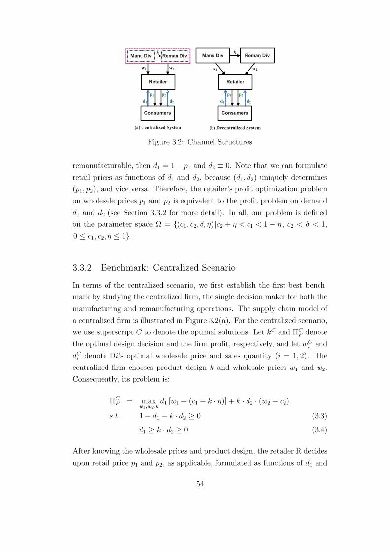
w1 w2

p1 p2

w1 w2

d1 d2

Reman DivManu Divk

Reman DivManu Div

Retailer

p1 p2

d1 d2

(a) Centralized System (b) Decentralized System

Consumers Consumers

Retailer

k

Figure 3.2: Channel Structures

remanufacturable, then d1 = 1− p1 and d2 ≡ 0. Note that we can formulate

retail prices as functions of d1 and d2, because (d1, d2) uniquely determines

(p1, p2), and vice versa. Therefore, the retailer’s profit optimization problem

on wholesale prices p1 and p2 is equivalent to the profit problem on demand

d1 and d2 (see Section 3.3.2 for more detail). In all, our problem is defined

on the parameter space Ω = (c1, c2, δ, η) |c2 + η < c1 < 1− η , c2 < δ < 1,

0 ≤ c1, c2, η ≤ 1.

3.3.2 Benchmark: Centralized Scenario

In terms of the centralized scenario, we first establish the first-best bench-

mark by studying the centralized firm, the single decision maker for both the

manufacturing and remanufacturing operations. The supply chain model of

a centralized firm is illustrated in Figure 3.2(a). For the centralized scenario,

we use superscript C to denote the optimal solutions. Let kC and ΠCF denote

the optimal design decision and the firm profit, respectively, and let wCi and

dCi denote Di’s optimal wholesale price and sales quantity (i = 1, 2). The

centralized firm chooses product design k and wholesale prices w1 and w2.

Consequently, its problem is:

ΠCF = max

w1,w2,kd1 [w1 − (c1 + k · η)] + k · d2 · (w2 − c2)

s.t. 1− d1 − k · d2 ≥ 0 (3.3)

d1 ≥ k · d2 ≥ 0 (3.4)

After knowing the wholesale prices and product design, the retailer R decides

upon retail price p1 and p2, as applicable, formulated as functions of d1 and

54

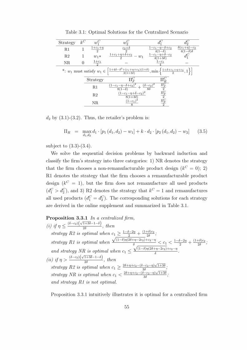
Table 3.1: Optimal Solutions for the Centralized Scenario

Strategy kC wC1 wC

2 dC1 dC2R1 1 1+c1+η

2c2+δ2

1−c1−η−δ+c24(1−δ)

δ(c1+η)−c24(1−δ)δ

R2 1 w1∗ 1+c1+η+δ+c22 − w1

1−c1−η+δ−c24(1+3δ) dC1

NR 0 1+c12 − 1−c1

4 −

*: w1 must satisfy w1 ∈[1+4δ−δ2+(c1+η+c2)(1+δ)

2(1+3δ) ,min

1+δ+c1+η+c22 , 1

]Strategy ΠC

F ΠCR

R1(1−c1−η−δ+c2)

2

8(1−δ) + (δ−c2)2

8δΠC

F2

R2(1−c1−η+δ−c2)2

8(1+3δ)

ΠCF2

NR(1−c1)

2

8ΠC

F2

d2 by (3.1)-(3.2). Thus, the retailer’s problem is:

ΠR = maxd1,d2

d1 · [p1 (d1, d2)− w1] + k · d2 · [p2 (d1, d2)− w2] (3.5)

subject to (3.3)-(3.4).

We solve the sequential decision problems by backward induction and

classify the firm’s strategy into three categories: 1) NR denotes the strategy

that the firm chooses a non-remanufacturable product design (kC = 0); 2)

R1 denotes the strategy that the firm chooses a remanufacturable product

design (kC = 1), but the firm does not remanufacture all used products

(dC1 > dC2 ), and 3) R2 denotes the strategy that kC = 1 and remanufactures

all used products (dC1 = dC2 ). The corresponding solutions for each strategy

are derived in the online supplement and summarized in Table 3.1.

Proposition 3.3.1 In a centralized firm,

(i) if η ≤ (δ−c2)(√1+3δ−1−δ)2δ

, then

strategy R2 is optimal when c1 ≥ 1−δ−2η2

+ (1+δ)c22δ

;

strategy R1 is optimal when

√(1−δ)η(2δ+η−2c2)+c2−η

δ< c1 <

1−δ−2η2

+ (1+δ)c22δ

;

and strategy NR is optimal when c1 ≤√

(1−δ)η(2δ+η−2c2)+c2−η

δ.

(ii) if η >(δ−c2)(

√1+3δ−1−δ)2δ

, then

strategy R2 is optimal when c1 ≥ 2δ+η+c2−(δ−c2−η)√1+3δ

3δ;

strategy NR is optimal when c1 <2δ+η+c2−(δ−c2−η)

√1+3δ

3δ;

and strategy R1 is not optimal.

Proposition 3.3.1 intuitively illustrates it is optimal for a centralized firm

55

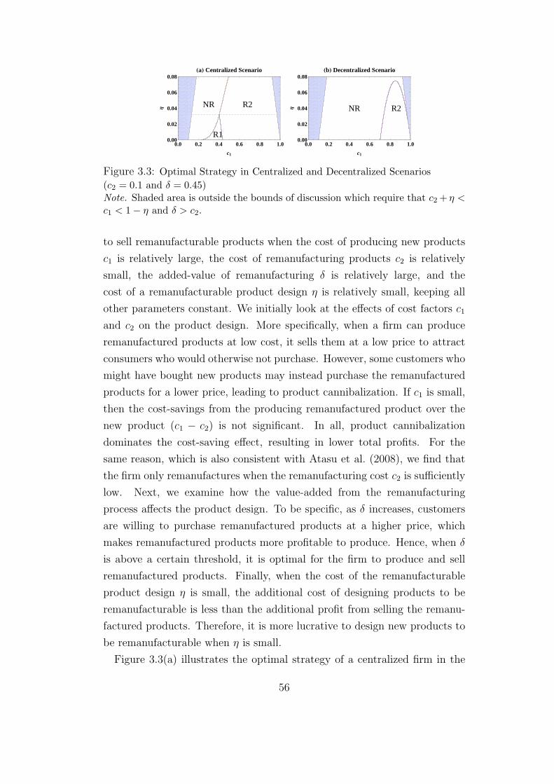
0.0 0.2 0.4 0.6 0.8 1.00.00

0.02

0.04

0.06

0.08

c1

Η

HaL Centralized Scenario

R1

R2NR

0.0 0.2 0.4 0.6 0.8 1.00.00

0.02

0.04

0.06

0.08

c1

Η

HbL Decentralized Scenario

NR R2

Figure 3.3: Optimal Strategy in Centralized and Decentralized Scenarios

(c2 = 0.1 and δ = 0.45)Note. Shaded area is outside the bounds of discussion which require that c2+ η <c1 < 1− η and δ > c2.

to sell remanufacturable products when the cost of producing new products

c1 is relatively large, the cost of remanufacturing products c2 is relatively

small, the added-value of remanufacturing δ is relatively large, and the

cost of a remanufacturable product design η is relatively small, keeping all

other parameters constant. We initially look at the effects of cost factors c1

and c2 on the product design. More specifically, when a firm can produce

remanufactured products at low cost, it sells them at a low price to attract

consumers who would otherwise not purchase. However, some customers who

might have bought new products may instead purchase the remanufactured

products for a lower price, leading to product cannibalization. If c1 is small,

then the cost-savings from the producing remanufactured product over the

new product (c1 − c2) is not significant. In all, product cannibalization

dominates the cost-saving effect, resulting in lower total profits. For the

same reason, which is also consistent with Atasu et al. (2008), we find that

the firm only remanufactures when the remanufacturing cost c2 is sufficiently

low. Next, we examine how the value-added from the remanufacturing

process affects the product design. To be specific, as δ increases, customers

are willing to purchase remanufactured products at a higher price, which

makes remanufactured products more profitable to produce. Hence, when δ

is above a certain threshold, it is optimal for the firm to produce and sell

remanufactured products. Finally, when the cost of the remanufacturable

product design η is small, the additional cost of designing products to be

remanufacturable is less than the additional profit from selling the remanu-

factured products. Therefore, it is more lucrative to design new products to

be remanufacturable when η is small.

Figure 3.3(a) illustrates the optimal strategy of a centralized firm in the

56

(c1, η) space for c2 = 0.1 and δ = 0.45. Note that (c1, η) in the upper left

and right corner does not satisfy our assumption; hence, it is beyond the

scope of our discussion. In general, when the firm designs new products to

be remanufacturable, it chooses strategy R2 over R1 when c1 is relatively

large, c2 is relatively small and δ is relatively large, keeping all other param-

eters constant. This is because the unit profit of selling one new product

decreases as c1 increases and the unit profit of selling one remanufactured

products increases as c2 decreases or as δ increases, making it profitable to

remanufacture as much as possible. As illustrated in Proposition 3.3.1(ii)

and Figure 3.3(a), it is not optimal for a firm to only remanufacture part of

the used products (strategy R1) when the cost of a remanufacturable product

design is not nominal (η >(δ−c2)(

√1+3δ−1−δ)2δ

). In particular, it can be shown

that(δ−c2)(

√1+3δ−1−δ)2δ

≤ 124. Thus, if η > 1

24, the firm should either design

the new products to be non-remanufacturable (strategy NR) or design them

to be remanufacturable and remanufacture all return products (strategy R2)

for any c1 and δ. Furthermore, the following corollary specifies the condition

when strategy NR is a dominating strategy:

Corollary 3.3.2 If η > 0 or c2 > 0, then there exists a threshold for c1 (δ)

above (below) which strategy NR is optimal.

According to Corollary 3.3.2, only when there is no extra cost to make new

products remanufacturable (η = 0) and there is no cost to remanufacture

(c2 = 0) will the firm always design new products to be remanufacturable, ir-

respective of the value of c1 and δ. This is because at “zero cost” (η = c2 = 0),

selling remanufactured products becomes so profitable that the loss in sales of

new products is easily compensated by the increase in sales of remanufactured

products. In fact, the firm is very likely to remanufacture as much as possible

(strategy R2) in such a case. To see this, based on Proposition 3.3.1, strategy

R2 is optimal when c1 ≥ 1−δ2

and R1 is optimal when c1 <1−δ2, where 1−δ

2< 1

2

since δ > 0. Nevertheless, as long as there is a cost to remanufacture or an

additional cost to make new products remanufacturable, it is not always

optimal for the firm to choose a remanufacturable product design.

In summary, a centralized firm chooses among three strategies: NR, R1 or

R2. A remanufacturable product design (R1 or R2) is optimal when the unit

production cost of new products (c1) is high, unit cost of remanufacturing

57

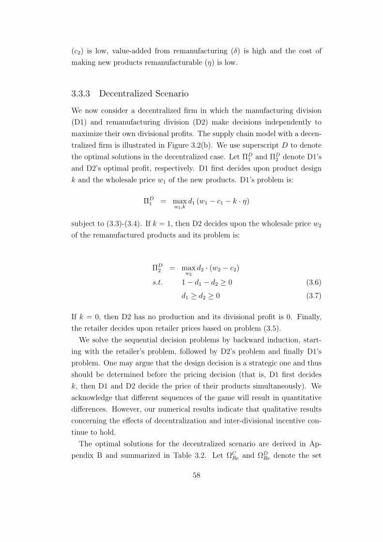
(c2) is low, value-added from remanufacturing (δ) is high and the cost of

making new products remanufacturable (η) is low.

3.3.3 Decentralized Scenario

We now consider a decentralized firm in which the manufacturing division

(D1) and remanufacturing division (D2) make decisions independently to

maximize their own divisional profits. The supply chain model with a decen-

tralized firm is illustrated in Figure 3.2(b). We use superscript D to denote

the optimal solutions in the decentralized case. Let ΠD1 and ΠD

2 denote D1’s

and D2’s optimal profit, respectively. D1 first decides upon product design

k and the wholesale price w1 of the new products. D1’s problem is:

ΠD1 = max

w1,kd1 (w1 − c1 − k · η)

subject to (3.3)-(3.4). If k = 1, then D2 decides upon the wholesale price w2

of the remanufactured products and its problem is:

ΠD2 = max

w2

d2 · (w2 − c2)

s.t. 1− d1 − d2 ≥ 0 (3.6)

d1 ≥ d2 ≥ 0 (3.7)

If k = 0, then D2 has no production and its divisional profit is 0. Finally,

the retailer decides upon retailer prices based on problem (3.5).

We solve the sequential decision problems by backward induction, start-

ing with the retailer’s problem, followed by D2’s problem and finally D1’s

problem. One may argue that the design decision is a strategic one and thus

should be determined before the pricing decision (that is, D1 first decides

k, then D1 and D2 decide the price of their products simultaneously). We

acknowledge that different sequences of the game will result in quantitative

differences. However, our numerical results indicate that qualitative results

concerning the effects of decentralization and inter-divisional incentive con-

tinue to hold.

The optimal solutions for the decentralized scenario are derived in Ap-

pendix B and summarized in Table 3.2. Let ΩCRe and ΩD

Re denote the set

58

Table 3.2: Optimal Strategy and Solutions for the Decentralized Scenario

Strategy kD Condition wD1 wD

2 dD1 dD2R2-1 1 ΩD

2−11+c1+η+δ−c2

21−c1−η+δ+c2

41−c1−η+δ−c2

8(1+3δ) dD1

R2-2 1 ΩD2−2 1 δ

2δ−c2

4(1+3δ) dD1

NR 0 ΩDNR

1+c12 − 1−c1

4 −

Strategy ΠD1 ΠD

2 ΠDR

R2-1 (1−c1−η+δ−c2)2

16(1+3δ)ΠD

1

2(1−c1−η+δ+c2)

2

64(1+3δ)

R2-2 (δ−c2)(1−c1−η)4(1+3δ)

(δ−c2)2

8(1+3δ)δ2

16(1+3δ)

NR (1−c1)2

8 − ΠD1

2

ΩD2−1 =

(c1, c2, δ, η)

∣∣∣∣ 1+5δ+η+c2−(δ−η−c2)√

2(1+3δ)

1+6δ≤ c1 ≤ 1− δ − η + c2

ΩD

2−2 = (c1, c2, δ, η)∣∣∣∣max

1− δ − η + c2,

1+2δ+c2−√

(δ−c2)(δ−2η−6δη−c2)

1+3δ

≤ c1

≤ 1+2δ+c2+√

(δ−c2)(δ−2η−6δη−c2)

1+3δ& η ≤ δ−c2

2(1+3δ)

ΩD

NR =(c1, c2, δ, η)

∣∣(c1, c2, δ, η) ∈ Ω− ΩD2−1 − ΩD

2−1

of (c1, c2, δ, η) such that a remanufacturable product design is optimal in

the centralized scenario (kC = 1) and the decentralized scenario (kD = 1),

respectively.

Proposition 3.3.3 For the decentralized firm,

(i) ΩDRe ⊂ ΩC

Re;

(ii) ΠD1 +ΠD

2 ≤ ΠCF , where the equality sign only holds when kC = 0; and

(iii) if (c1, c2, δ, η) ∈ ΩDRe, then dD1 = dD2 < dC1 , d

D1 + dD2 < dC1 + dC2 .

Proposition 3.3.3(i) indicates that a remanufacturable product design is

less likely to be chosen in the decentralized scenario than in the central-

ized scenario. This is consistent with our intuition because although a

remanufacturable product design benefits the remanufacturing division, it

not only cannibalizes the sales of new products (as is illustrated in part (iii)

of Proposition 3.3.3), but it also incurs an additional unit cost η to D1,

both adversely affecting D1’s profit. Another reason is that in a centralized

firm, the design decision is optimized by comparing the firm’s total profit

with and without a remanufacturable product design. On the contrary, in

a decentralized firm, the design decision is optimized by comparing D1’s

profit with and without a remanufacturable product design. Note that the

firm’s total profit without a remanufacturable product design in a centralized

scenario equals D1’s profit without a remanufacturable product design in the

decentralized scenario while the firm’s total profit with a remanufacturable

59

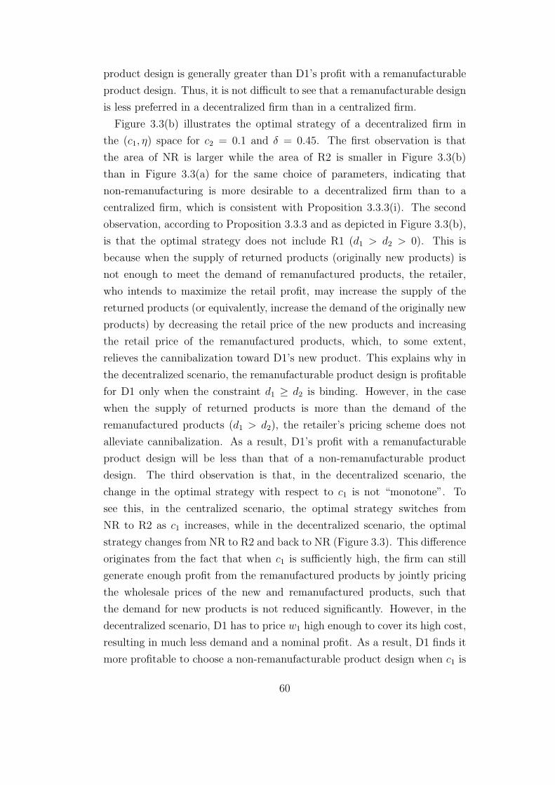
product design is generally greater than D1’s profit with a remanufacturable

product design. Thus, it is not difficult to see that a remanufacturable design

is less preferred in a decentralized firm than in a centralized firm.

Figure 3.3(b) illustrates the optimal strategy of a decentralized firm in

the (c1, η) space for c2 = 0.1 and δ = 0.45. The first observation is that

the area of NR is larger while the area of R2 is smaller in Figure 3.3(b)

than in Figure 3.3(a) for the same choice of parameters, indicating that

non-remanufacturing is more desirable to a decentralized firm than to a

centralized firm, which is consistent with Proposition 3.3.3(i). The second

observation, according to Proposition 3.3.3 and as depicted in Figure 3.3(b),

is that the optimal strategy does not include R1 (d1 > d2 > 0). This is

because when the supply of returned products (originally new products) is

not enough to meet the demand of remanufactured products, the retailer,

who intends to maximize the retail profit, may increase the supply of the

returned products (or equivalently, increase the demand of the originally new

products) by decreasing the retail price of the new products and increasing

the retail price of the remanufactured products, which, to some extent,

relieves the cannibalization toward D1’s new product. This explains why in

the decentralized scenario, the remanufacturable product design is profitable

for D1 only when the constraint d1 ≥ d2 is binding. However, in the case

when the supply of returned products is more than the demand of the

remanufactured products (d1 > d2), the retailer’s pricing scheme does not

alleviate cannibalization. As a result, D1’s profit with a remanufacturable

product design will be less than that of a non-remanufacturable product

design. The third observation is that, in the decentralized scenario, the

change in the optimal strategy with respect to c1 is not “monotone”. To

see this, in the centralized scenario, the optimal strategy switches from

NR to R2 as c1 increases, while in the decentralized scenario, the optimal

strategy changes from NR to R2 and back to NR (Figure 3.3). This difference

originates from the fact that when c1 is sufficiently high, the firm can still

generate enough profit from the remanufactured products by jointly pricing

the wholesale prices of the new and remanufactured products, such that

the demand for new products is not reduced significantly. However, in the

decentralized scenario, D1 has to price w1 high enough to cover its high cost,

resulting in much less demand and a nominal profit. As a result, D1 finds it

more profitable to choose a non-remanufacturable product design when c1 is

60

0.2 0.3 0.4 0.5 0.6 0.7 0.8 0.90

20

40

60

80

100

Pro

fit L

oss

(%)

0.2 0.3 0.4 0.5 0.6 0.7 0.8 0.90

20

40

60

80

100

Dem

and

Loss

(%

)

0.2 0.3 0.4 0.5 0.6 0.7 0.8 0.9

Cen

tral

.

0.2 0.3 0.4 0.5 0.6 0.7 0.8 0.9c

1

Dec

entr

al.

NR R1 R2

NR R2−2

Figure 3.4: Centralized Firm vs. Decentralized Firm (c2=0.1, δ = 0.45 and

η = 0.01)

relatively high.

Propositions 3.3.3(ii) and 3.3.3(iii) suggest that, even in the case when it is

optimal for the manufacturing division to choose a remanufacturable product

design, the total profit ΠDF = ΠD

1 + ΠD2 and total demand dD1 + dD2 of the

decentralized firm are both strictly less than that of the centralized firm. As

an outcome of decentralization, D1 increases w1 and D2 decreases w2 to max-

imize their own divisional profit, respectively, leading to a suboptimal profit

and sales for the firm. Figure 3.4 depicts the effects of decentralization on

total profit, total demand and the optimal strategy when c2 = 0.1, δ = 0.45

and η = 0.01. The first two subfigures in Figure 3.4 provide the ratio of profit

loss (1− ΠDF

ΠCF) and sales loss (1− dD1 +dD2

dC1 +dC2) due to decentralization as c1 varies,

which can be as high as 51% and 46%, respectively. Such a drastic negative

decentralization effect usually occurs when the optimal strategy changes from

R2 to NR (see the last two subfigures, which illustrates the optimal strategies

in the centralized and decentralized scenarios, respectively).

As illustrated in Proposition 3.3.3, cost ownership and product cannibal-

ization foil D1’s remanufacturable product design, and thus, result in a lower

total profit than the firm-wide benchmark profit ΠCF . Therefore, it is in

a decentralized firm’s best interest to introduce a coordination mechanism

and to incentivize D1 to design new products to be remanufacturable. A

natural conjecture would be that the firm achieves coordination by making

D2 responsible for all or a portion of the cost associated with a remanu-

61

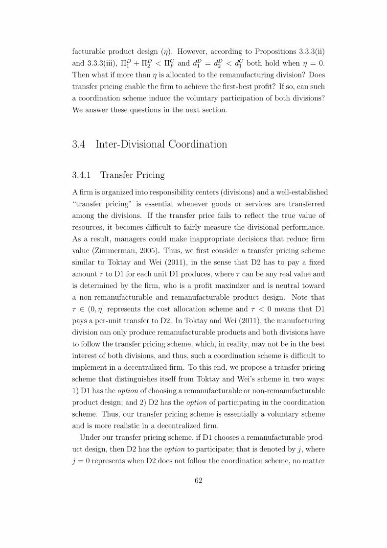
facturable product design (η). However, according to Propositions 3.3.3(ii)

and 3.3.3(iii), ΠD1 + ΠD

2 < ΠCF and dD1 = dD2 < dC1 both hold when η = 0.

Then what if more than η is allocated to the remanufacturing division? Does

transfer pricing enable the firm to achieve the first-best profit? If so, can such

a coordination scheme induce the voluntary participation of both divisions?

We answer these questions in the next section.

3.4 Inter-Divisional Coordination

3.4.1 Transfer Pricing

A firm is organized into responsibility centers (divisions) and a well-established

“transfer pricing” is essential whenever goods or services are transferred

among the divisions. If the transfer price fails to reflect the true value of

resources, it becomes difficult to fairly measure the divisional performance.

As a result, managers could make inappropriate decisions that reduce firm

value (Zimmerman, 2005). Thus, we first consider a transfer pricing scheme

similar to Toktay and Wei (2011), in the sense that D2 has to pay a fixed

amount τ to D1 for each unit D1 produces, where τ can be any real value and

is determined by the firm, who is a profit maximizer and is neutral toward

a non-remanufacturable and remanufacturable product design. Note that

τ ∈ (0, η] represents the cost allocation scheme and τ < 0 means that D1

pays a per-unit transfer to D2. In Toktay and Wei (2011), the manufacturing

division can only produce remanufacturable products and both divisions have

to follow the transfer pricing scheme, which, in reality, may not be in the best

interest of both divisions, and thus, such a coordination scheme is difficult to

implement in a decentralized firm. To this end, we propose a transfer pricing

scheme that distinguishes itself from Toktay and Wei’s scheme in two ways:

1) D1 has the option of choosing a remanufacturable or non-remanufacturable

product design; and 2) D2 has the option of participating in the coordination

scheme. Thus, our transfer pricing scheme is essentially a voluntary scheme

and is more realistic in a decentralized firm.

Under our transfer pricing scheme, if D1 chooses a remanufacturable prod-

uct design, then D2 has the option to participate; that is denoted by j, where

j = 0 represents when D2 does not follow the coordination scheme, no matter

62

whether it remanufactures or not (note if D2 remanufactures but does not

participate, then the problem is essentially equivalent to the decentralized

problem without the incentive discussed in Section 3.3.3). In addition, j = 1

represents when D2 follows the coordination scheme and remanufactures the

returned products. In the latter case, D2 pays a variable amount τ to D1

for each unit D1 produces. Note that if D1 designs new products to be non-

remanufacturable (k = 0), then D2’s profit is always 0 and hence no transfer

occurs. We use the superscript V to denote the optimal solutions in the

presence of the transfer pricing scheme. Given the transfer pricing scheme

and the region ΩCRe, D1’s problem becomes ΠV

1 = maxw1,k

d1(w1−c1−k·η+j ·k·τ)subject to constraints (3.3)-(3.4). If k = 1, then D2’s problem becomes

ΠV2 = max

w2,jd2 · (w2 − c2) − j · d1 · τ subject to constraints (3.6)-(3.7). The

retailer’s problem remains the same as formulated by (3.5).

Now, given the transfer pricing scheme, will both divisions voluntarily join

the coordination program? The success of such an inter-divisional coordi-

nation requires the profit of both divisions to be greater than when in the

absence of an incentive (the decentralized scenario in Section 3.3.3). That is,

ΠV1 ≥ ΠD

1 and ΠV2 ≥ ΠD

2 (referred to as “participation constraints”) whenever

the coordination scheme exists, where ΠV1 and ΠV

2 denote D1 and D2’s profits

with the option of design/coordination, respectively. Based on the numerical

results, we make the following observations.

Observation 1 Given (c1, c2, δ, η) ∈ ΩCR2, there exists a τV such that the

first-best optimal firm profit can be achieved (i.e., ΠV1 + ΠV

2 = ΠCF ) when

τ = τV . Moreover, ΠV2 = ΠD

2 , ΠV1 > ΠD

2 , dVi = dCi (i = 1, 2) and τV > 0.

Observation 1 reveals that under the transfer pricing scheme, the decen-

tralized firm can always achieve the optimal total profit and optimal sales

level of both new and remanufactured products (if applicable) as in the

centralized scenario when (c1, c2, δ, η) ∈ ΩCR2, where ΩC

R2 is a subset of ΩCRe.

Recall that decentralization can result in a lower profit and fewer sales, as

stated in Propositions 3.3.3(ii) and (iii). Thus, the transfer pricing scheme

benefits the firm in both aspects. Correspondingly, D2’s profit is the same

as in the decentralized scenario without incentive and D1’s profit increases

ΠCF − ΠV

2 − ΠV1 > 0. In other words, in the equilibrium, D2’s participation

constraint ΠV2 ≥ ΠD

2 is always binding while D1’s participation constraint

63

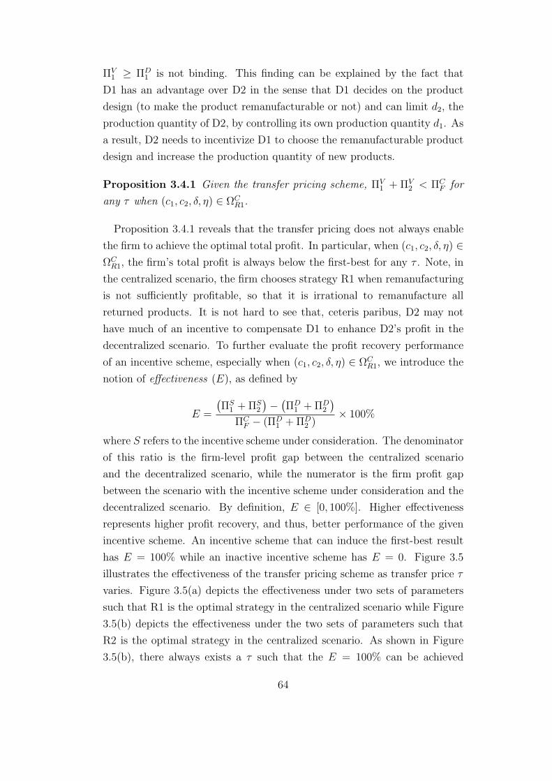
ΠV1 ≥ ΠD

1 is not binding. This finding can be explained by the fact that

D1 has an advantage over D2 in the sense that D1 decides on the product

design (to make the product remanufacturable or not) and can limit d2, the

production quantity of D2, by controlling its own production quantity d1. As

a result, D2 needs to incentivize D1 to choose the remanufacturable product

design and increase the production quantity of new products.

Proposition 3.4.1 Given the transfer pricing scheme, ΠV1 + ΠV

2 < ΠCF for

any τ when (c1, c2, δ, η) ∈ ΩCR1.

Proposition 3.4.1 reveals that the transfer pricing does not always enable

the firm to achieve the optimal total profit. In particular, when (c1, c2, δ, η) ∈ΩC

R1, the firm’s total profit is always below the first-best for any τ . Note, in

the centralized scenario, the firm chooses strategy R1 when remanufacturing

is not sufficiently profitable, so that it is irrational to remanufacture all

returned products. It is not hard to see that, ceteris paribus, D2 may not

have much of an incentive to compensate D1 to enhance D2’s profit in the

decentralized scenario. To further evaluate the profit recovery performance

of an incentive scheme, especially when (c1, c2, δ, η) ∈ ΩCR1, we introduce the

notion of effectiveness (E), as defined by

E =

(ΠS

1 +ΠS2

)−

(ΠD

1 +ΠD2

)ΠC

F − (ΠD1 +ΠD

2 )× 100%

where S refers to the incentive scheme under consideration. The denominator

of this ratio is the firm-level profit gap between the centralized scenario

and the decentralized scenario, while the numerator is the firm profit gap

between the scenario with the incentive scheme under consideration and the

decentralized scenario. By definition, E ∈ [0, 100%]. Higher effectiveness

represents higher profit recovery, and thus, better performance of the given

incentive scheme. An incentive scheme that can induce the first-best result

has E = 100% while an inactive incentive scheme has E = 0. Figure 3.5

illustrates the effectiveness of the transfer pricing scheme as transfer price τ

varies. Figure 3.5(a) depicts the effectiveness under two sets of parameters

such that R1 is the optimal strategy in the centralized scenario while Figure

3.5(b) depicts the effectiveness under the two sets of parameters such that

R2 is the optimal strategy in the centralized scenario. As shown in Figure

3.5(b), there always exists a τ such that the E = 100% can be achieved

64

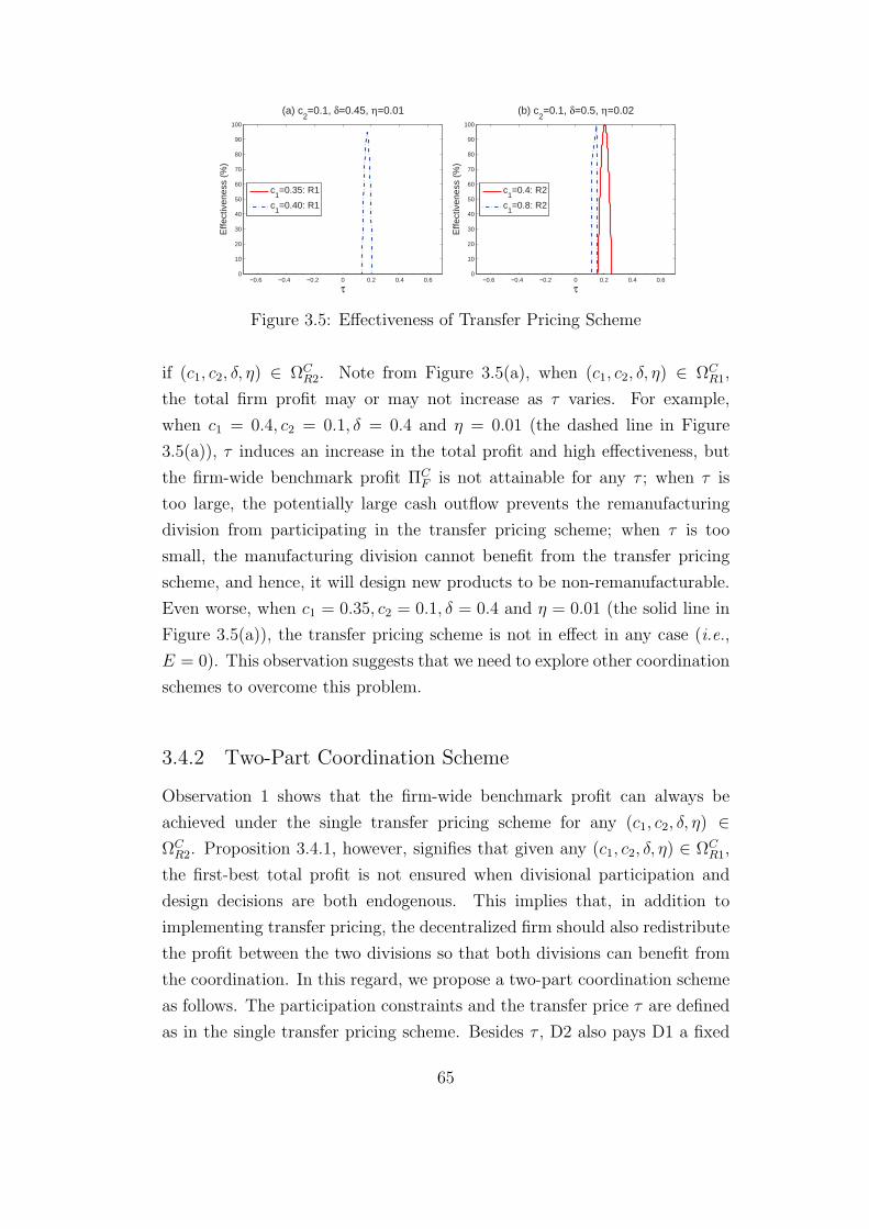
−0.6 −0.4 −0.2 0 0.2 0.4 0.60

10

20

30

40

50

60

70

80

90

100

τ

Effe

ctiv

enes

s (%

)

(a) c2=0.1, δ=0.45, η=0.01

c1=0.35: R1

c1=0.40: R1

−0.6 −0.4 −0.2 0 0.2 0.4 0.60

10

20

30

40

50

60

70

80

90

100

τ

Effe

ctiv

enes

s (%

)

(b) c2=0.1, δ=0.5, η=0.02

c1=0.4: R2

c1=0.8: R2

Figure 3.5: Effectiveness of Transfer Pricing Scheme

if (c1, c2, δ, η) ∈ ΩCR2. Note from Figure 3.5(a), when (c1, c2, δ, η) ∈ ΩC

R1,

the total firm profit may or may not increase as τ varies. For example,

when c1 = 0.4, c2 = 0.1, δ = 0.4 and η = 0.01 (the dashed line in Figure

3.5(a)), τ induces an increase in the total profit and high effectiveness, but

the firm-wide benchmark profit ΠCF is not attainable for any τ ; when τ is

too large, the potentially large cash outflow prevents the remanufacturing

division from participating in the transfer pricing scheme; when τ is too

small, the manufacturing division cannot benefit from the transfer pricing

scheme, and hence, it will design new products to be non-remanufacturable.

Even worse, when c1 = 0.35, c2 = 0.1, δ = 0.4 and η = 0.01 (the solid line in

Figure 3.5(a)), the transfer pricing scheme is not in effect in any case (i.e.,

E = 0). This observation suggests that we need to explore other coordination

schemes to overcome this problem.

3.4.2 Two-Part Coordination Scheme

Observation 1 shows that the firm-wide benchmark profit can always be

achieved under the single transfer pricing scheme for any (c1, c2, δ, η) ∈ΩC

R2. Proposition 3.4.1, however, signifies that given any (c1, c2, δ, η) ∈ ΩCR1,

the first-best total profit is not ensured when divisional participation and

design decisions are both endogenous. This implies that, in addition to

implementing transfer pricing, the decentralized firm should also redistribute

the profit between the two divisions so that both divisions can benefit from

the coordination. In this regard, we propose a two-part coordination scheme

as follows. The participation constraints and the transfer price τ are defined

as in the single transfer pricing scheme. Besides τ , D2 also pays D1 a fixed

65

Table 3.3: Comparison of Coordination Schemes

Scheme Transfer Pricing Fixed Lump-sum Two-part Scheme

Condition ΩCR1 ΩC

R2 ΩCR1 ΩC

R2 ΩCR1 ΩC

R2

Achieve Opt.? No Yes No Yes Yes Yes

Payer of τopt n/a D2 n/a n/a D1 D1/D2

Payer of fopt n/a n/a n/a D2 D2 D1/D2

Robustness n/a Sensitive n/a Robust SensitiveSensitive w.r.t τRobust w.r.t f

τ opt(fopt): optimal τ(f) that induces the first-best result.

amount f . f is determined by the firm and is independent of the sales

of new or remanufactured products. Note that f can be any real value,

where a negative f means that D1 pays a lump sum to D2. In addition, no

transfer, variable or fixed, occurs should D1 design new products to be non-

remanufacturable. We use superscript T to denote the optimal solutions in

the presence of the two-part coordination scheme. As such, D1’s problem is

ΠT1 = max

w1,kd1(w1−c1−k ·η+j ·k ·τ)+k ·j ·f subject to constraints (3.3)-(3.4).

If k = 1, then D2’s problem becomes ΠT2 = max

w2,jd2 · (w2− c2)− j ·d1 · τ − j · f

subject to constraints (3.6)-(3.7).

Recall that the participation constraints are ΠT1 ≥ ΠD

1 and ΠT2 ≥ ΠD

2 .

However, the two-part coordination scheme allows for weaker “participation

constraints” ΠT1 +ΠT

2 > ΠD1 +ΠD

2 because the lump sum f reallocates the total

profit and is allowed to be any value, positive or negative. The comparison of

transfer pricing (τ), fixed lump-sum scheme (f) and two-part scheme (τ, f)

is summarized in Table 3.3. We will discuss Table 3.3 in more detail below.

Proposition 3.4.2 In the presence of the two-part coordination scheme,

(i) τT = c1+η−12

< 0, ΠT1 = fT > 0 and total transfer dT1 · τT + fT ≥ 0

when (c1, c2, δ, η) ∈ ΩCR1;

(ii) there exists some fT > 0 such that τT = 0 when (c1, c2, δ, η) ∈ ΩCR2;

and

(iii) ΠTF = ΠC

F , ΩTRi = ΩC

Ri and dTi = dCi (i = 1, 2) for any (c1, c2, δ, η).

Proposition 3.4.2 indicates that the benefits of our proposed internal in-

centive to a decentralized firm are twofold. On the one hand, the incentive

can always enable the firm to achieve the optimal firm-wide profit and sales

level as in the centralized scenario for any parameter set (c1, c2, δ, η). By

66

contrast, as is illustrated in the first row of Table 3.3, the single-parameter

scheme cannot guarantee the first-best result. On the other hand, the internal

incentive motivates D1 to choose a remanufacturable product design as if

it were the planner in a centralized firm. Recall that new products are

designed to be remanufacturable in fewer cases due to decentralization, as

stated in Proposition 3.3.3(i). Therefore, the two-part coordination scheme

encourages the manufacturing division in a decentralized firm to choose a

remanufacturable product design.

Moreover, Proposition 3.4.2 has two interesting implications. First, one

would expect τ to be positive, because D1, who determines design decision

k, has more “power” over D2, and thus, D2 would have to compensate D1 for

choosing a remanufacturable product design. However, when (c1, c2, δ, η) ∈ΩC

R1, it is actually optimal for D1 to “compensate” D2 in the amount of τT

for each new unit D1 produces (τT < 0). Note that product cannibalization

is prominent when (c1, c2, δ, η) ∈ ΩCR1. Under such a circumstance, the per-

unit transfer τT from D1 to D2 motivates D2 to raise the wholesale prices

of the remanufactured products (w2 = δ(w1−τ)+c22

, as shown in the proof of

Proposition 3.4.2), and thus, alleviates the side effects of cannibalization on

the sales of new products, which is beneficial to D1. Proposition 3.4.2(i)

highlights that if τ is restricted to be non-negative, then the first-best firm

profit cannot always be achieved. In particular, a fixed lump-sum scheme

without a transfer price (i.e., τ = 0) generally fails to induce the first-best

result, because f cannot affect the optimal wholesale prices. In addition, D2

has to pay D1 a lump sum fT > 0, because ΠT1 = fT when (c1, c2, δ, η) ∈

ΩCR1. To determine fT , recall that the participation constraint ΠT

1 ≥ ΠD1 , or

equivalently fT ≥ ΠD1 , needs to be satisfied while ΠD

1 ≥ (1−c1)2

8> 0, according

to Table 3.2. Thus, D2 will have to make a fixed transfer fT > 0 to motivate

D1 to voluntarily design new products to be remanufacturable. Also note

that wT1 + τT = c1 + η and fT ≥ 0 are consistent with the literature on

franchising that suggests selling at the marginal cost and charging franchise

fees to achieve channel coordination (Cachon and Lariviere 2005). In our

context, although D1 does not literally sell new products to D2, a portion of

D1’s products will be collected by D2 and becomes D2’s production input. In

some sense, D1 “sells” new products to D2, who later sells them in the form of

remanufactured products. Therefore, franchising theory can still be applied.

In particular, the total transfer should be positive so that the manufacturing

67

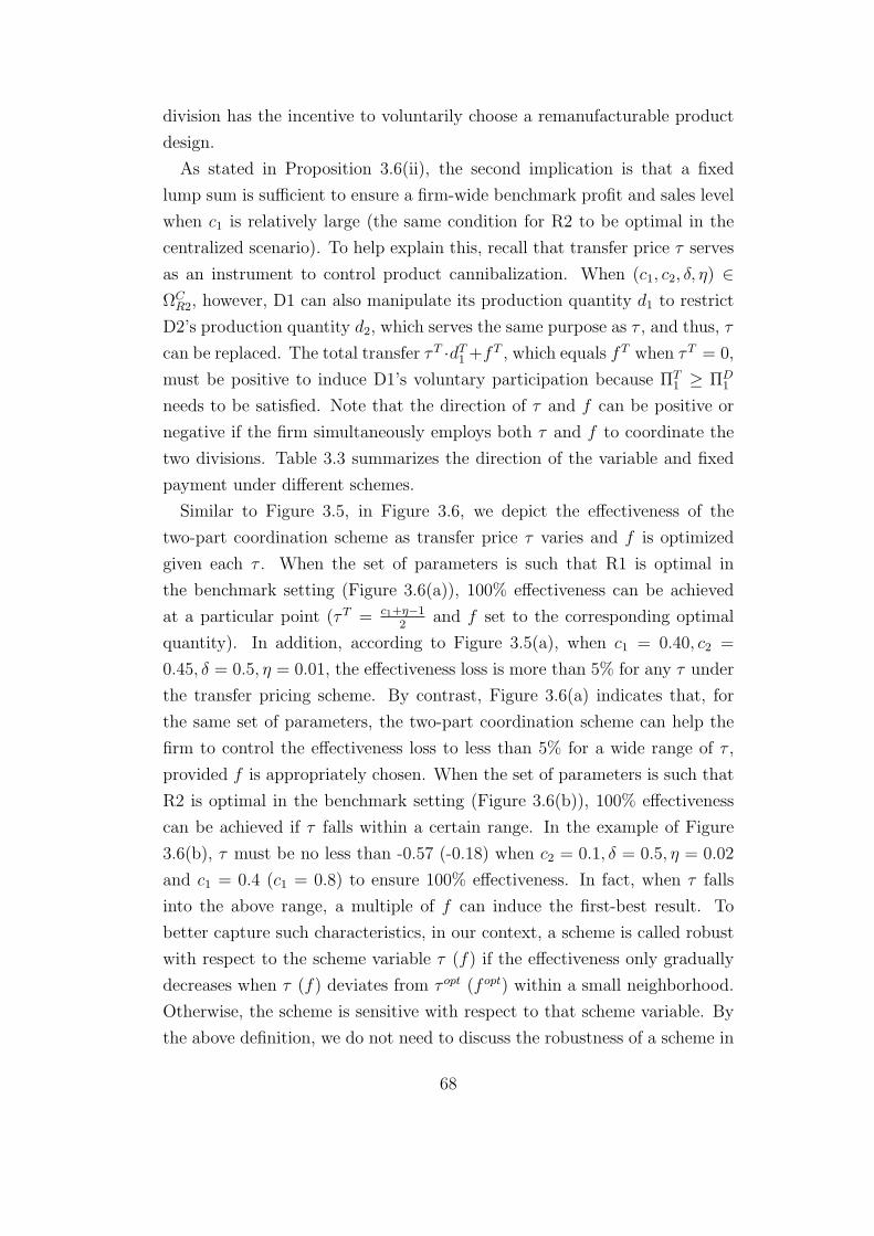
division has the incentive to voluntarily choose a remanufacturable product

design.

As stated in Proposition 3.6(ii), the second implication is that a fixed

lump sum is sufficient to ensure a firm-wide benchmark profit and sales level

when c1 is relatively large (the same condition for R2 to be optimal in the

centralized scenario). To help explain this, recall that transfer price τ serves

as an instrument to control product cannibalization. When (c1, c2, δ, η) ∈ΩC

R2, however, D1 can also manipulate its production quantity d1 to restrict

D2’s production quantity d2, which serves the same purpose as τ , and thus, τ

can be replaced. The total transfer τT ·dT1 +fT , which equals fT when τT = 0,

must be positive to induce D1’s voluntary participation because ΠT1 ≥ ΠD

1

needs to be satisfied. Note that the direction of τ and f can be positive or

negative if the firm simultaneously employs both τ and f to coordinate the

two divisions. Table 3.3 summarizes the direction of the variable and fixed

payment under different schemes.

Similar to Figure 3.5, in Figure 3.6, we depict the effectiveness of the

two-part coordination scheme as transfer price τ varies and f is optimized

given each τ . When the set of parameters is such that R1 is optimal in

the benchmark setting (Figure 3.6(a)), 100% effectiveness can be achieved

at a particular point (τT = c1+η−12

and f set to the corresponding optimal

quantity). In addition, according to Figure 3.5(a), when c1 = 0.40, c2 =

0.45, δ = 0.5, η = 0.01, the effectiveness loss is more than 5% for any τ under

the transfer pricing scheme. By contrast, Figure 3.6(a) indicates that, for

the same set of parameters, the two-part coordination scheme can help the

firm to control the effectiveness loss to less than 5% for a wide range of τ ,

provided f is appropriately chosen. When the set of parameters is such that

R2 is optimal in the benchmark setting (Figure 3.6(b)), 100% effectiveness

can be achieved if τ falls within a certain range. In the example of Figure

3.6(b), τ must be no less than -0.57 (-0.18) when c2 = 0.1, δ = 0.5, η = 0.02

and c1 = 0.4 (c1 = 0.8) to ensure 100% effectiveness. In fact, when τ falls

into the above range, a multiple of f can induce the first-best result. To

better capture such characteristics, in our context, a scheme is called robust

with respect to the scheme variable τ (f) if the effectiveness only gradually

decreases when τ (f) deviates from τ opt (f opt) within a small neighborhood.

Otherwise, the scheme is sensitive with respect to that scheme variable. By

the above definition, we do not need to discuss the robustness of a scheme in

68

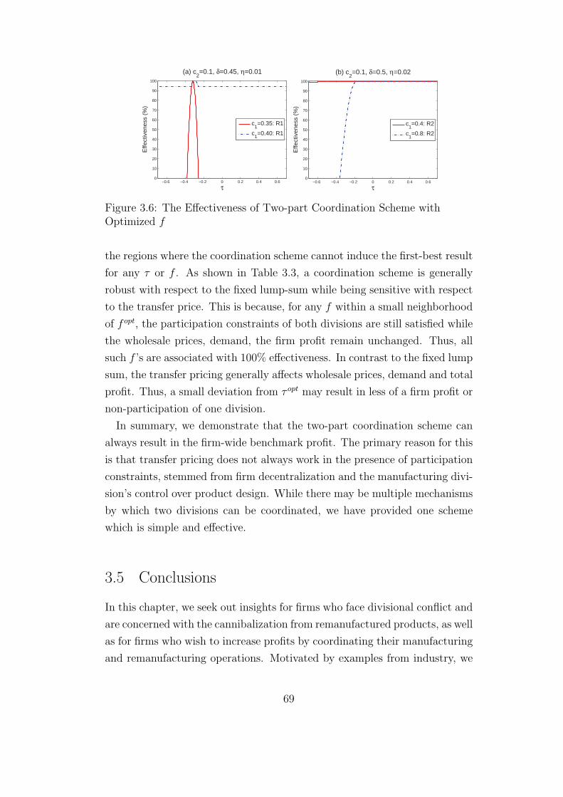
−0.6 −0.4 −0.2 0 0.2 0.4 0.60

10

20

30

40

50

60

70

80

90

100

τ

Effe

ctiv

enes

s (%

)

(a) c2=0.1, δ=0.45, η=0.01

c1=0.35: R1

c1=0.40: R1

−0.6 −0.4 −0.2 0 0.2 0.4 0.60

10

20

30

40

50

60

70

80

90

100

τ

Effe

ctiv

enes

s (%

)

(b) c2=0.1, δ=0.5, η=0.02

c1=0.4: R2

c1=0.8: R2

Figure 3.6: The Effectiveness of Two-part Coordination Scheme withOptimized f

the regions where the coordination scheme cannot induce the first-best result

for any τ or f . As shown in Table 3.3, a coordination scheme is generally

robust with respect to the fixed lump-sum while being sensitive with respect

to the transfer price. This is because, for any f within a small neighborhood

of f opt, the participation constraints of both divisions are still satisfied while

the wholesale prices, demand, the firm profit remain unchanged. Thus, all

such f ’s are associated with 100% effectiveness. In contrast to the fixed lump

sum, the transfer pricing generally affects wholesale prices, demand and total

profit. Thus, a small deviation from τ opt may result in less of a firm profit or

non-participation of one division.

In summary, we demonstrate that the two-part coordination scheme can

always result in the firm-wide benchmark profit. The primary reason for this

is that transfer pricing does not always work in the presence of participation

constraints, stemmed from firm decentralization and the manufacturing divi-

sion’s control over product design. While there may be multiple mechanisms

by which two divisions can be coordinated, we have provided one scheme

which is simple and effective.

3.5 Conclusions

In this chapter, we seek out insights for firms who face divisional conflict and

are concerned with the cannibalization from remanufactured products, as well

as for firms who wish to increase profits by coordinating their manufacturing

and remanufacturing operations. Motivated by examples from industry, we

69

consider a firm consisting of a manufacturing division and a remanufacturing

division, and a retailer through whom the firm sells all of its products.

Given this construct, we explore the optimal strategy with respect to design

architecture and pricing in centralized and decentralized scenarios. We find

that it is optimal for the centralized firm to undertake remanufacturing with

a high production cost of new products, a low remanufacturing cost, a high

value-added from remanufacturing, and a low cost of the remanufacturable

product design. However, the manufacturing division of the decentralized

firm would be more likely to choose a non-remanufacturing design to avoid

a potential increase in production cost and competition from the remanufac-

tured products. By comparing the two scenarios, we demonstrate that firm

decentralization and divisional conflict reduce both profits and total sales;

in addition, they prevent the firm from offering a remanufacturable product

design. Therefore, it is to the firm’s advantage to implement inter-divisional

coordination mechanism to improve overall performance.

Thus, we investigate several incentive mechanisms that coordinate a firm’s

manufacturing and remanufacturing divisions. Motivated by Toktay and Wei

(2011), we first examine the effectiveness of transfer pricing. We show that

transfer pricing cannot always induce the remanufacturable product design

or the first-best profits because the participation constraints of the manufac-

turing and remanufacturing divisions cannot be satisfied simultaneously. In

fact, this occurs when it is optimal for a firm to remanufacture only a fraction

of the returned products in the centralized scenario. Thus, the decentralized

firm should not only use the transfer price to achieve the highest profit. To

probe deeper, we propose an inter-divisional coordination scheme, with a

transfer price for each unit the manufacturing division produces and a fixed

lump sum payment that is independent of the sales of new or remanufactured

products. We prove that this two-part coordination scheme always enables

the firm to invariably achieve the first-best total profit and sales level and

can effectively promote a remanufacturable product design. An interesting

finding is that the inter-divisional transfer is not always from the remanufac-

turing division to the manufacturing division. We illustrate that, in the case

when it is optimal to remanufacture only a fraction of the used products

in the centralized scenario, a two-parameter inter-divisional coordination

scheme with a per-unit transfer from the manufacturing division to the

remanufacturing division and a lump sum payment from the remanufacturing

70

division to the manufacturing division is required to achieve the first-best

outcome. However, in the case when remanufacturing is sufficiently profitable

so that it is optimal to remanufacture all used products in the centralized

scenario, a one-parameter incentive with either a lump sum or a transfer

price paid by the remanufacturing division to the manufacturing division

is sufficient. The reason is that product cannibalization can be managed

through production quantity control. Finally, we find that the fixed lump-

sum scheme performs more robustly than the transfer price.

Our results and discussions are based, in part, on the modeling stipulation

that the wholesale prices of new and remanufactured products must be no

more than the maximum customer WTP (i.e., w1, w2 ≤ 1). Although this

assumption seems plausible, we find that it is not always optimal for the firm

to price new products below the maximum customer WTP. We considered,

as a modeling extension, the case when wholesale prices are allowed to exceed

the maximum customer WTP. The most noticeable observation is that the

decentralized firm is more likely to choose a remanufacturable product design

without a price constraint than with a price constraint, which implies that

under certain circumstance, the manufacturing division can increase its profit

by designing new products to be remanufacturable and selling them to the

retailer at a price that is higher than the maximum customer WTPs. The

explanation is that, in some cases, selling remanufactured products is so

profitable that the retailer is willing to adjust the retail price of new products

to be less than the maximum customer WTP (and bear the loss from the

new products) in order to guarantee enough returns for remanufacturing.

Essentially, the manufacturing division extracts profit from the retailer and

the remanufacturing division by optimally pricing new products, even if the

price is above the maximum customer WTP.

So far, our discussion is limited to the case of a firm selling all products

to its end-users through a retailer. In practice, some companies integrate

retailing (vertical integration) and sell both new and remanufactured prod-

ucts directly to their end-users. Therefore, we also study the role of a

retailer in a closed-loop supply chain by comparing the firm’s optimal pricing,

product design for remanufacturing and profitability with and without an

independent retailer. We find that in the centralized scenario, the firm’s profit

and the demand for new and remanufactured products (if applicable) doubles

when the firm integrates retailing because vertical integration completely

71

eliminates double marginalization. By contrast, in the decentralized scenario,

vertical disintegration benefits the firm in terms of both sales quantity and

profit and encourages the manufacturing division to undertake a remanufac-

turable product design, which is because the retailer’s optimal pricing scheme

alleviates product cannibalization and the manufacturing division can extract

additional surplus from the retailer. Therefore, in the absence of an inde-

pendent retailer, the manufacturing division will always design new products

to be non-remanufacturable in order to avoid product cannibalization, the

production cost increase, and potential profit loss. In all, to maximize profit

and boost sales, the centralized firm should consider retail integration while

the decentralized firm should strategically disintegrate retailing.

In closing, we acknowledge that our discussion is restricted to the situation

of when all used products can be returned and remanufactured and when the

collection cost is negligible. Considering that lower return and remanufactur-

ing rates and a higher collection cost should lead to less of a cannibalization

risk for the decentralized firm, our model focuses on the most unfavorable

conditions for remanufacturing operations.

72

CHAPTER 4

THE EFFECTS OF PATENT TERMEXTENSION AND PHARMACEUTICALSTEWARDSHIP PROGRAM ON GREEN

PHARMACY

“The future will be green, or not at all.”

– Jonathon Espie Porritt.

4.1 Introduction

The issue of potential environmental impact by pharmaceuticals has gained

increasing attention in the last two decades. Since the 1980s, a number of

studies have examined the origin, occurrence and consequence of pharma-

ceuticals and personal care products (PPCPs) in surface, subsurface, and

drinking waters (see reviews by Halling-Sørensen et al. 1998, Daughton 2001

and Tong et al. 2011). For example, the studies by Kidd et al. (2007) and

Vajda et al. (2008) showed the feminization of male fish and female-biased sex

ratio as the result of freshwater exposure to synthetic estrogenic substances

(source of female sex hormones) in Ontario, Canada and Colorado, U.S.,

respectively. Another example is the veterinary use of the nonsteroidal anti-

inflammatory drug diclofenac, which resulted in catastrophic decline of three

vulture species of Gyps in Southeast Asia (Oaks et al. 2004). Kolpin et al.

(2002) found that pharmaceuticals, hormones, and other organic wastewater

contaminants were present in over 80% of the streams sampled across the

United States. The occurrence of PPCPs as trace environmental pollutants

is primarily originated from consumer use and actions rather than leaks in the

manufacturing process (Daughton 2003a). The U.S. Centers for Medicare &

Medicaid Services (CMS) and the Department of Health and Human Services

(DHHS) estimate that $406.1 billion will be spent on prescription drugs in

2020 (CMS/DHHS 2014), among which 10 to 33 percent will be unused

(Grasso et al. 2009). Another survey by Trueman et al. (2010) suggested

73

that the annual primary and community care prescription medicines wastage

in England costs about GB£300 million, accounting for 4% of the medication

cost.

The main causes for waste include, among other things, early recovery

before all dispensed medicines are taken, ineffectiveness or unwanted side ef-

fects, prescription change by the physicians, non-adherence and non-compliance

with drug treatment. (Morgan 2001, Ruhoy and Daughton 2008, Trueman

et al. 2010). Unwanted pharmaceuticals can reach the environment when

disposed in the garbage, toilet or sink. In fact, in a study conducted by

Kotchen et al. (2009), 73.2% of 1005 households in the central coast of

California threw unused medications in the rubbish or flushed them down

the toilet or sink. Only 11% of the sampled households returned unused

medications to a pharmacy or dropped them off at a hazardous waste center.

With the deteriorating situation of eco-toxicity of pharmaceuticals and

mixtures of medicines, the U.S. Environmental Protection Agency (U.S.

EPA), the European Environment Agency (EEA), and many other orga-

nizations are advancing the practice of “green pharmacy” (Daughton 2003a,

2003c, EEA 2010). According to EEA, green pharmacy is the design of

pharmaceutical products and processes that eliminates or reduces the use

and generation of hazardous substances (EEA 2010). In other words, green

pharmacy focuses on the innovation of “benign by design” drugs while keep-

ing the safety and efficacy of the drug unaffected by the innovation.

Pharmaceutical companies are now taking steps to pursue green phar-

macy. For instance, Schering-Plough Pharmaceuticals, LLC modified its

birth control products by using natural estrogens paired with a biodegradable

progesterone (Lubick, 2008). Major pharmaceutical companies, as well as

policymakers and scientists, are gathering to discuss how to make drugs more

environmentally friendly at conventions such as the International Conference

on Sustainable Pharmacy and the American Chemical Society’s Green Insti-

tute Pharmaceutical Roundtable (Knoblauch 2009).

A major obstacle in achieving green pharmacy is the high R&D expense

of inventing green pharmaceuticals or redesigning existing products to be

greener by identifying or using biodegradable ingredients or agents. To

alleviate this, one possible incentive is to offer patent term extension to

pharmaceutical companies that formulate greener drugs. The award of a

patent allows an inventor to temporarily and exclusively use its invention,

74

and the importance of patents is significant to the pharmaceutical sector

(Mansfield et al. 1981, Competition DG, 2009). Currently, pharmaceutical

companies may obtain patent extension with new formulation, new routes of

administration for known drugs, stereoselectivity or chiral switches, new uses,

fixed-dose combinations, polymorphism (Kvesic 2008, Gupta et al. 2010).

But none of these reasons is related to green pharmacy. EEA, however, has

proposed the idea of implementing patent extension to encourage pharmaceu-

tical companies to develop substances with less environmental impact (EEA

2010). Given the ever-growing costs of drug development, such incentive

can encourage the consideration of degradable green drugs (Shah 2010),

foster stewardship programs that tie both environmental and human health

together (Daughton 2003b), and help make green pharmacy a part of the

company’s strategic plan (Clark et al. 2010), especially for the innovative

company. In addition, the patent system not only helps to stimulate inno-

vation, but also encourages technical information disclosure (Merges 1988).

If patent extension can be awarded to advance green pharmacy, then green

technology can be easily and widely implemented after the patent expiration.

As highlighted above, patent incentives could stimulate pharmaceutical

companies to invest in green pharmacy. Thus, in this chapter, we answer

the following questions: Under what conditions can the implementation of

a pharmaceutical patent term extension induce green pharmacy? What are

the impacts of the patent term extension on environmental performance,

the availability of pharmaceutics, and the profitability of the firms? What

is the optimal length of patent extension? To this end, we consider an

innovative company who collects monopoly profits for its patented medicine

and faces competition from a generic rival after the patent expires. Both

the innovative company and the generic company maximize their own prof-

its. Their products, if not appropriately disposed of, could exert negative

impact on the environment. Both firms can achieve green pharmacy and

thus reduce adverse environmental impact by investing a fixed amount. In

the case when the innovative company obtains patent extension by investing

in green pharmacy, the generic rival can take a free-ride after the extended

patent expired. To determine the optimal extended patent term, we assume

that the regulator considers two stakeholders: the number of patients who

cannot afford the pharmaceutical products, and the potential contamination

of unwanted pharmaceuticals to the surface, subsurface, and drinking waters.

75

We demonstrate that a patent term extension can encourage the innovative

company to invest in green pharmacy. In particular, the patent incentive is

effective when fixed investment cost is low, the extended term of the patent

is long or competition intensity is high. In fact, the more competitive is

the market, the more is the innovative company willing to invest in green

pharmacy, even under shorter extended terms of the patent. As a result,

the regulator can induce green pharmacy with a short extended term when

market competition is intensive. Specifically, the optimal extended term is

finite when the regulator is seeking the balance of the affordability of medicine

and the environmental protection; in general, a longer extended term is

needed to induce green pharmacy when the fixed investment cost increases.

Nevertheless, we also show that implementing the patent term extension

can be suboptimal, especially when the regulator values the affordability of

medicines over environmental stewardship.

Another possible approach for the regulator to promote green pharmacy

is to impose a pharmaceutical take-back program. Similar to the product

stewardship programs for items such as electronics and beverage containers,

residents would be able to deliver their unused medicines to appropriate

entities for safe and effective disposal; and drug manufacturers would be

required to run and pay for the program. Pharmaceutical take-back pro-

grams exist in many countries, such as Canada (Health Products Stewardship

Association), Australia (Return Unwanted Medicines Project), and most

countries in Europe (EEA 2010). In the U.S., the Alameda County Safe

Drug Disposal Ordinance, first adopted in June, 2012, is a first-in-the-nation

pharmaceutical extended producer responsibility program, and was upheld

by the U.S. Court of Appeals for the Ninth Circuit in September, 2014.

Heidi Sanborn of the California Product Stewardship Council pointed out

that shifting responsibility for drug waste to manufacturers could lead to

greener design in terms of “what it’s made out of, how it works, (and) how

long it lasts” (Bartolone 2014).

Thus, in this chapter, we also address the following questions: which

environmental policy is more effective in inducing green pharmacy, the patent

term extension, the take-back regulation, or the combination of both? In-

tuitively, when both companies are subject to the take-back regulation and

the compliance cost associated with the take-back regulation is independent

of the choice of green pharmacy, pharmaceutical companies will neither go

76

green nor bear all the compliance cost; some of the environmental cost will

eventually be transferred to the consumers. Furthermore, we demonstrate

that adding the take-back regulation on top of the patent term extension

can potentially reduce firm profit and generally require a longer extended

patent term. Yet, we also conclude that the combined policy outperforms the

patent term extension when the compliance cost is relatively small, the fixed

investment cost and the collection rate are relatively large, the competition is

either nominal or sufficiently intensive, and the environmental issue is rather

urgent.

To address the issue that the take-back regulation alone cannot promote

green pharmacy, we propose a modified take-back policy such that com-

panies with green pharmacy pay a lower compliance cost per unit than if

without green pharmacy. Compared with the patent term extension that

can only motivate the innovative company to invest in green pharmacy, the

modified take-back regulation can sometimes encourage both companies to

invest. Also, the modified take-back regulation is better than the patent

extension when the competition intensity is relatively high. Last, when

implementing a combined policy of both patent term extension and take-

back regulation, using the modified cost structure is typically superior to the

traditional cost structure. Interestingly, under this modified combined policy,

the innovative company may find it profitable to go green without requesting

patent extension. The intuition here is that company is not obliged to reveal

the ingredients or process of green pharmacy, which alleviates competition

from the generics by exclusively enjoying the benefits of green pharmacy it

invents. However, implementing only the patent term extension can generate

less social and environmental impact than a combined policy when the needs

of pharmaceuticals are compelling or when the compliance cost is relatively

large.

The rest of this chapter is organized as follows. We first review related

literature in Section 4.2. In Section 4.3, we formally define the green phar-

macy, patent term extension and pharmaceuticals take-back regulations, and

introduce some main assumptions. In Section 4.4, we study the patent

term extension by developing the decision model and establishing properties

of its optimal solution. Then, in Section 4.5, we explore implications of

the take-back regulation. In Section 4.6, we study how compliance cost

structure affects the optimal strategy of the pharmaceutical companies and

77

the regulator. Section 4.7 concludes this chapter and discusses the scope

and limitation of this study. The proofs of propositions, lemmas, and the

corollary are provided in Appendix C.

4.2 Relation to Literature

Our study is related to three streams of literature. First, a fast-growing

stream of works in operations management addresses the issues related to

product take-back regulations (e.g., Toyasaki et al. 2011, Atasu and Subra-

manian 2012, Atasu et al. 2013, Gui et al. 2013). In particular, a number

of researchers studied how the take-back regulation affects product design

decisions of manufacturers (e.g., Zuidwijk and Krikke 2008, Plambeck and

Wang 2009, Esenduran and Kemahlıoglu-Ziya 2015). However, a pharmaceu-

tical stewardship program is different from traditional product stewardship

programs in several ways. First, the goal of a pharmaceutical stewardship

program is not only to reduce pharmaceuticals in the environment but to

reduce drug abuse and accidental poisoning as well. The second difference is

that the reverse channel of pharmaceutical products is still strictly regulated,

especially for controlled substances. For example, the Disposal of Controlled

Substances Final Rule by the U. S. Drug Enforcement Administration (DEA)

stated that a person may not dispose pharmaceutical controlled substances

for a non-member of her household and that controlled substance can only be

returned to a DEA authorized collector (DEA 2014). The third difference is

that a pharmaceutical stewardship program can hardly bring any economic

benefit to the participating pharmaceutical companies because pharmaceuti-

cal products have almost no end-of-life value. In fact, such a program usually

requires that pharmaceutical products be safely disposed of through certified

incineration. As a result, regulations or incentives are needed to ensure

the implementation of a pharmaceuticals take-back program. We contribute

to this literature by extending the analysis of the take-back regulation to

pharmaceuticals.

The second stream of literature explores the interactions between patent,

price and innovation (e.g., Kitch 1977, Gilbert and Shapiro 1990, Jaffe 2000).

In the pharmaceutical industry, relevant studies surged after the Drug Price

Competition and Patent Term Restoration Act of 1984 (known as the “Hatch-

78

Waxman Act”) was implemented (e.g., Grabowski and Vernon 1992, Bottazzi

et al. 2001, Lee 2003). In this study, we focus on the role of patent term

extension in the investment and development of environmentally friendly

pharmaceutical substances, as suggested by EEA (2010). We believe that no

study has been conducted to validate this proposal. Hence, there is a clear

need for research to analyze and compare the patent term extension with

other existing regulatory policy. In this study, we make the first attempt and

obtain guidelines for choosing the optimal length of the patent extension.

Finally, our study is related to the literature that examines the choice of

the policy instruments and the efficiency implication of regulatory policies

on the environment (e.g., Palmer and Walls 1997, Calcott and Walls 2000,

Walls 2006, Krass et al. 2013). Our study differs from theirs in several ways.

First, we consider patent term extension as a policy instrument to induce

environmentally friendly design, which has rarely been studied before. Patent

protection is critical to the pharmaceutical industry, and thus has a high

potential for realizing the goal of environmental protection. Second, in this

chapter, the availability of pharmaceuticals is an important consideration

for the regulators. Pharmaceuticals differ from other commodities in that

consumer surplus or producer surplus is not as crucial as the number of people

who cannot afford the drug. Therefore, we incorporate the affordability

rather than consumer surplus into the model of the regulator. Third, we also

propose a new compliance cost structure that relates the unit compliance cost

to the choice of green pharmacy. The traditional compliance cost structure

fails to promote sustainable product design because it is independent of the

greenness of products. We conclude that our proposed cost scheme typically

achieves better performance than the traditional one.

To the best of our knowledge, the only other study that employs oper-

ations approaches to analyze extended producer responsibility (EPR) for

pharmaceuticals is the working paper by Alev et al. (2013), who investigate

the effectiveness of EPR policies by considering the interactions between

doctors, patients, manufacturers and insurance companies; however, they do

not explore patent term extension as a regulatory tool nor do they examine

the role of green pharmacy in product design.

79

4.3 Green Pharmacy, Patent Term Extension, and

Take-back Regulation Defined

In this section, we define the terms, notation, and assumptions that lay

the groundwork for our models. Specifically, we first formalize our no-

tions of green pharmacy, patent term extension, and take-back regulations.

Then, we specify several assumptions regarding the market segments, cost

structure, and the goals of pharmaceutical companies and regulator. Table

4.1 summarizes the technical notation and assumptions discussed in this

chapter. And Figure 4.1 illustrates the decisions of the innovative and generic

pharmaceutical companies under different policies.

4.3.1 Defining Green Pharmacy

Consistent with the concept proposed by the U.S. EPA and EEA (Daughton

2003a, 2003c, EEA 2010), we mean for green pharmacy to represent the

redesign of a pharmaceutical product such that the generation of hazardous

substances is reduced while the two fundamental traits of the pharmaceutical

product, i.e., safety and efficacy, remain unchanged. Thus, the environmental

impact of one unit of the green product per period is only α fraction of the

environmental impact of one unit of the non-green counterpart per period,

where α ∈ [0, 1) reflects the degree of non-greenness. A small α denotes green

pharmacy that results in little environmental impact.

The definition of green pharmacy implicitly assumes that the customer de-

mand is independent of the greenness of pharmacy because the two essential

traits of the pharmaceutical product remain constant. Moreover, in reality,

customers have little access to the environmental hazard assessments of each

pharmaceutical product. One exception is the database of regional envi-

ronmental classification system for pharmaceuticals set up by the Stockholm

County Council, Sweden in 2003 (http://www.janusinfo.se/Beslutsstod/Miljo-

och-lakemedel/About-the-environment-and-pharmaceuticals/Environmentially-

classified-pharmaceuticals/). Unfortunately, such database is not available

in the global sense.

80

4.3.2 Defining Patent and Patent Term Extension

In our model, the innovative company is granted a patent for a limited period

of time for its invention of the brand name drug, and the invention is subject

to public disclosure after the expiration of the patent. For simplicity, we do

not differentiate “patent” with “exclusivity”. For detailed difference, readers

can refer to http://www.fda.gov/Drugs/DevelopmentApprovalProcess/

ucm079031.htm. Therefore, in our setting, the innovative company is the

monopoly, and the brand name drug is the only available drug in the market

as long as the patent protection is active. However, after the patent expires, a

generic company will immediately enter the market and produce the generic

version of the brand name drug based on the public disclosure.

The patent term extension is used restrictively in this chapter to refer to the

extended term of a granted patent for the development of green pharmacy by

the innovative company. According to our assumption, only the innovative

company may be granted patent term extension. The regulator has the

option of implementing patent term extension, which is known to both the

innovative and generic companies before they make decisions. If patent term

extension exists and the innovative company develops green pharmacy, then

the innovative company is granted an n-period patent extension. Thus,

within the extended n periods, the innovative company can still charge the

monopoly price. Note the generic company can obtain the ingredients of

green drug, free of charge, after the patent expires if the innovative company

develops a green drug and receives patent extension. However, we assume

that the generic company cannot obtain green pharmacy, free of charge, if

the innovative company develops a green drug without applying for patent

extension. We will relax this assumption and discuss its implication in the

conclusion section.

4.3.3 Defining Take-back Regulations

To encourage pharmaceutical companies to take responsibility for pharma-

ceutical waste, the regulator may consider adopting pharmaceuticals take-

back regulations. The pharmaceuticals take-back regulations require that

pharmaceutical producers create and finance a collection and disposal pro-

gram for unused/wasted medicines. Existing pharmaceutical companies pay

81

for all administrative and operational expenses of running the program based

on their market share. In fact, collection and disposal operations are funded

in part by manufacturers based on prior year’s sales volumes in France

(Wisconsin DNR 2012) and on market share in Canada (Product Stewardship

Institute 2011). In the presence of the take-back regulation, the compliance

cost for a pharmaceutical company is ct · d, where d is the sales of that

company.

4.3.4 Key Assumptions

Assumption 1: The regulator chooses environmental policy by weighting

two considerations: the non-affordability of pharmaceuticals (social impact)

and the generation of hazardous substances (environmental impact).

The regulator decides whether to implement an environmental policy by

taking two stakeholders into consideration. First, the number of patients

who cannot afford the pharmaceutical products. Expensive medicines could

jeopardize lives and result in adverse social impact. We assume that the social

impact associated with unaffordable pharmaceutical products is e1(1−d1−d2)

per period, where the market size is normalized to 1; d1 and d2 are the sales

of the brand name and generic name drugs, respectively. Second, unused and

expired pharmaceuticals products that are not collected could contaminate

surface, subsurface, and drinking waters (Daughton 2003a). We assume that

τ × 100% of sales will be unused, of which (1− η) × 100% can be collected

and safely disposed of if the take-back regulation exists, where τ, η ∈ [0, 1].

Assume that environmental impact per period is E per unit of non-green

product (in monetary terms) and αE per unit of green products (in monetary

terms). Thus, the total environmental impact of unsafe disposal per period is

αl · e2d if the take-back regulation does not exist and ηαle2d if the regulation

exists, where d is the sales of a pharmaceutical company, e2 = Eτ , l = 1 if the

pharmaceutical product is green, and l = 0 if the pharmaceutical product

is not green. We acknowledge that collection and disposal of unused and

wasted medicine result in at least some greenhouse gas (GHG) emissions

(Wisconsin DNR 2012) and that active pharmaceutical ingredients (APIs)

can be introduced to sewage as a result of excretion and bathing (Ruhoy and

Daughton 2008). However, we ignore these two impacts to help us focus on

82

the two major stakeholders.

Assumption 2: The green pharmacy is achievable no earlier than T0, the

time when the original patent expires.

Both companies can obtain green pharmacy (and thus produce green drugs)

for a one-time R&D fixed cost of A at T0 is assumed to be A. In practice, the

effective period of patent protection can hardly be more than 8 years because,

in general, manufacturers start applying for patent protection before they

perform clinical trials on a compound (Gassmann et al. 2008). Considering

that few manufacturers would want to develop greener version of the drug

before they can market and sell the original version, we assume that green

drugs become available at T0. As a result, we only need to consider the

cumulative payoff for all periods after the original patent expires (referred to

hereafter as T0).

Assumption 3: The demand curve slopes down. Generic drugs can can-

nibalize the sales of brand name drugs but brand name awareness/brand

loyalty exists.

A number of empirical studies indicate that a 1 percent increase in the price

of prescription drugs will lead to a 0.15-0.33 percent decrease in the number

of prescriptions in the United Kingdom (O’Brien 1989, Lavers 1989). In

the presence of a cost-sharing prescription drug plan, the price elasticity of

demand is still negative though the absolute value decreases (Harris et al.

1990, Smith 1993). In addition, innovator brand loyalty in pharmaceuticals

has been observed and analyzed in many previous studies (Scherer and Ross

1990, Grabowski and Vernon 1992, Frank and Salkever 1992). This can be

explained by the fact that brand name companies spend more on advertise-

ments (Hurwitz and Caves 1988) and that patients have the experience or

perception of low risk and high efficacy of brand name medicines (Denoth

et al. 2011, Meredith 2003). The empirical study by Kjoenniksen et al. (2006)

found that 41% of the patients would not switch to generic drugs should they

have no personal economic incentives.

As a result, we assume that the pharmaceutical product market is cross-

price-sensitive. If a customer’s willing-to-pay (wtp) for the brand name drug

is θ, then her wtp for the generic product is δ · θ, where δ ∈ [0, 1) and

θ is distributed uniformly between 0 and 1. δ < 1 not only reflects the

fact that patients are willing to pay more for brand name drugs, but also

captures the intensity of the market competition. δ close to 0 represents no

83

competition (brand name medicine dominates the market) while δ close to

1 represents an extremely intensive competition. Assume that a customer

maximizes her customer surplus (wtp less the price) and makes a purchase

only if her customer surplus is positive. In the same spirit as Moorthy (1984),

the demand for the brand name and generic drug per period is d1 = 1− p1−p21−δ

and d2 = δp1−p2(1−δ)δ

, respectively when both drugs are available in the market.

It is not hard to derive that before patent expiration, the monopoly demand

(demand for the brand name drug) per period is dm = 1− pm.

Assumption 4: The per unit cost to produce brand name drug or generic

drug is c0 = 0.

We normalize the manufacturing cost to zero because the unit production

cost usually has marginal impact on the pricing of drugs and, therefore, is

sometimes negligible. For example, a hepatitis C drug called Sovaldi is priced

at $84,000 but the manufacturing cost is only $150 (Jogalekar, 2014).

Assumption 5: The per unit compliance cost of the take-back regulations

ct is less than δ2and is independent of whether a company adopts green

pharmacy.

We restrict our discussion to the case when ct ≤ δ2for two reasons. First,

the administrative and operational expenses of running the program must be

within a reasonable and affordable range for both the innovative company

and the generic company. In particular, it is not profitable for the generic

companies to enter the market when ct ≥ δ. Second, this assumption allows

us to focus on the interior optimal solutions and to avoid discussing the

boundary condition.

4.4 Patent Term Extension and Model Solutions

Based on the terms, notations and assumptions introduced in Section 4.3, we

use this section to formulate the models of the pharmaceutical companies in

response to the given environmental policy (policy N or E), and the model

of the regulator given the optimal response of the companies.

84

Innov: p1; G1 or O

Generic: p2; G1 or O

Policy incl.

Patent Extension?

Innov: G0?

Innov: pm; G0

Innov: p1; G0

Generic: p2; F

No

No

Yes

Yes

Figure 4.1: Decisions of Pharmaceutical Companies under Different policies

4.4.1 The Model of the Pharmaceutical Companies

4.4.1.1 Benchmark Model: No Regulatory Policy (Policy N)

Given policy N , the innovative company decides whether to pursue green

pharmacy and the price of its brand name drug p1 at time T0. The profit of

the innovative company is Π1 = maxp1

11−r

· 1−δ−p1+p21−δ

· p1 − A if it goes green

(denoted as strategy G1) and Π1 = maxp1

11−r

· 1−δ−p1+p21−δ

· p1 if it does not

go green (denoted as strategy O). Meanwhile, the generic company decides

whether to invest in green pharmacy and the price of the generic drug p2.

The profit of the generic company is Π2 = maxp2

11−r

· δp1−p2(1−δ)δ

· p2 − A if it goes

green (strategy G1) and Π2 = maxp2

11−r

· δp1−p2(1−δ)δ

· p2 if it does not go green

(strategy O). It is not hard to see that neither company has an incentive

to invest in green pharmacy under this policy. By solving the simultaneous

game, we have the following results:

Lemma 4.4.1 In the absence of the patent term extension (policy N), (O,O)

is the equilibrium. Moreover, ΠN1 = 4(1−δ)

(1−r)(4−δ)2, ΠN

2 = (1−δ)δ

(1−r)(4−δ)2, pN1 = 2(1−δ)

4−δ,

pN2 = (1−δ)δ4−δ

, dN1 = 24−δ

, and dN2 = 14−δ

.

Lemma 4.4.1 is consistent with intuition because by choosing green phar-

macy, pharmaceutical companies incur a fixed cost without any benefits un-

der policy N . Thus, in the absence of any regulatory policy, pharmaceutical

companies will not invest to go green. Also, due to the brand loyalty, the

85

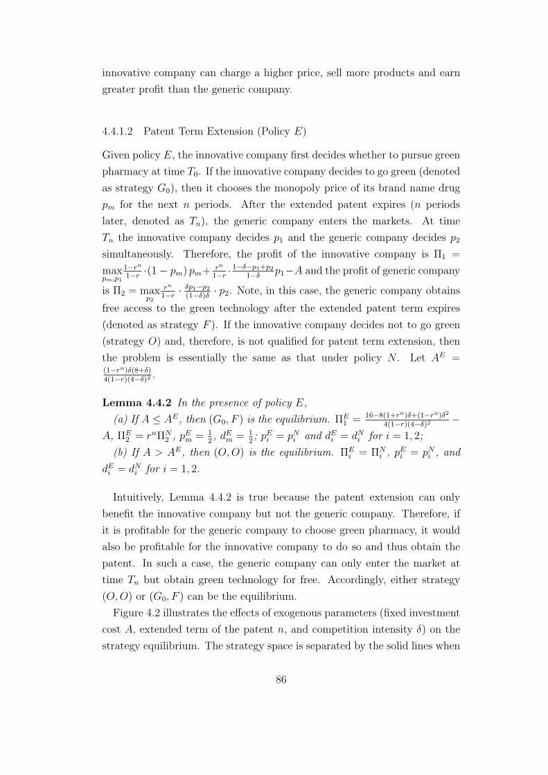
innovative company can charge a higher price, sell more products and earn

greater profit than the generic company.

4.4.1.2 Patent Term Extension (Policy E)

Given policy E, the innovative company first decides whether to pursue green

pharmacy at time T0. If the innovative company decides to go green (denoted

as strategy G0), then it chooses the monopoly price of its brand name drug

pm for the next n periods. After the extended patent expires (n periods

later, denoted as Tn), the generic company enters the markets. At time

Tn the innovative company decides p1 and the generic company decides p2

simultaneously. Therefore, the profit of the innovative company is Π1 =

maxpm,p1

1−rn

1−r·(1− pm) pm+ rn

1−r· 1−δ−p1+p2

1−δp1−A and the profit of generic company

is Π2 = maxp2

rn

1−r· δp1−p2

(1−δ)δ· p2. Note, in this case, the generic company obtains

free access to the green technology after the extended patent term expires

(denoted as strategy F ). If the innovative company decides not to go green

(strategy O) and, therefore, is not qualified for patent term extension, then

the problem is essentially the same as that under policy N . Let AE =(1−rn)δ(8+δ)4(1−r)(4−δ)2

.

Lemma 4.4.2 In the presence of policy E,

(a) If A ≤ AE, then (G0, F ) is the equilibrium. ΠE1 = 16−8(1+rn)δ+(1−rn)δ2

4(1−r)(4−δ)2−

A, ΠE2 = rnΠN

2 , pEm = 1

2, dEm = 1

2; pEi = pNi and dEi = dNi for i = 1, 2;

(b) If A > AE, then (O,O) is the equilibrium. ΠEi = ΠN

i , pEi = pNi , and

dEi = dNi for i = 1, 2.

Intuitively, Lemma 4.4.2 is true because the patent extension can only

benefit the innovative company but not the generic company. Therefore, if

it is profitable for the generic company to choose green pharmacy, it would

also be profitable for the innovative company to do so and thus obtain the

patent. In such a case, the generic company can only enter the market at

time Tn but obtain green technology for free. Accordingly, either strategy

(O,O) or (G0, F ) can be the equilibrium.

Figure 4.2 illustrates the effects of exogenous parameters (fixed investment

cost A, extended term of the patent n, and competition intensity δ) on the

strategy equilibrium. The strategy space is separated by the solid lines when

86

0.1 0.2 0.3 0.40.0

0.2

0.4

0.6

0.8

1.0

A

∆

n=6

n=2

HO,OL

HG0,FL

Figure 4.2: Equilibrium under Policy E (r = 0.8)

n = 2 and by the dashed lines when n = 6. First, when fixed investment

cost A is sufficiently small, the innovative company chooses to invest in green

pharmacy to prolong the patent and monopoly; when A is sufficiently large,

the innovative company will not go green because the benefit of extended

patent cannot justify the cost of investment. Second, a longer extended

term of the patent (larger n) makes investment in green pharmacy more

attractive for the innovative company because innovative company can charge

monopoly price and earns monopoly profit for a longer time. Last, a high

degree of competition intensity encourages investment in green pharmacy,

which is intuitive because green pharmacy allows the innovative company

to exclusively possess the market for an additional n periods. In a similar

vein, as the competition becomes more intensive, the innovative company is

willing to go green in order to take advantage of the patent extension even

with higher investment cost A or shorter extended term of the patent n.

4.4.2 The Model of the Regulator – Implement the PatentTerm Extension (E) or Not (N)?

To decide whether it is optimal for the regulator to implement the patent

term extension, we need to compare the resulting social and environmental

impacts under policy N with those under policy E. Recall that (O,O) is the

equilibrium for any A under policy N (see Lemma 4.4.1) and for A > AE

under policy E (see Lemma 4.4.2), which indicates that patent term extension

cannot induce green pharmacy and, therefore, does not change the social and

environmental impact when A > AE. Consequently, we only need to focus

on the case when A ≤ AE.

87

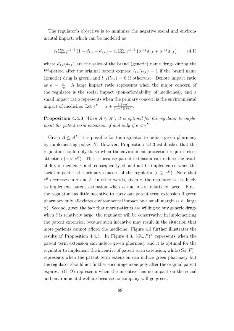
The regulator’s objective is to minimize the negative social and environ-

mental impact, which can be modeled as

e1Σ∞k=1r

k−1 (1− d1,k − d2,k) + e2Σ∞k=1r

k−1(αl1,kd1,k + αl2,kd1,k

)(4.1)

where d1,k(d2,k) are the sales of the brand (generic) name drugs during the

kth-period after the original patent expires; l1,k(l2,k) = 1 if the brand name

(generic) drug is green, and l1,k(l2,k) = 0 if otherwise. Denote impact ratio

as e = e1e2. A large impact ratio represents when the major concern of

the regulator is the social impact (non-affordability of medicines), and a

small impact ratio represents when the primary concern is the environmental

impact of medicine. Let eE = α + 6(1−α)(1−rn)(2+δ)

.

Proposition 4.4.3 When A ≤ AE, it is optimal for the regulator to imple-

ment the patent term extension if and only if e < eE.

Given A ≤ AE, it is possible for the regulator to induce green pharmacy

by implementing policy E. However, Proposition 4.4.3 establishes that the

regulator should only do so when the environment protection requires close

attention (e < eE). This is because patent extension can reduce the avail-

ability of medicines and, consequently, should not be implemented when the

social impact is the primary concern of the regulator (e ≥ eE). Note that

eE decreases in α and δ. In other words, given e, the regulator is less likely

to implement patent extension when α and δ are relatively large. First,

the regulator has little incentive to carry out patent term extension if green

pharmacy only alleviates environmental impact by a small margin (i.e., large

α). Second, given the fact that more patients are willing to buy generic drugs

when δ is relatively large, the regulator will be conservative in implementing

the patent extension because such incentive may result in the situation that

more patients cannot afford the medicine. Figure 4.3 further illustrates the

results of Proposition 4.4.3. In Figure 4.3, (G0, F )+ represents when the

patent term extension can induce green pharmacy and it is optimal for the

regulator to implement the incentive of patent term extension, while (G0, F )−

represents when the patent term extension can induce green pharmacy but

the regulator should not further encourage monopoly after the original patent

expires. (O,O) represents when the incentive has no impact on the social

and environmental welfare because no company will go green.

88

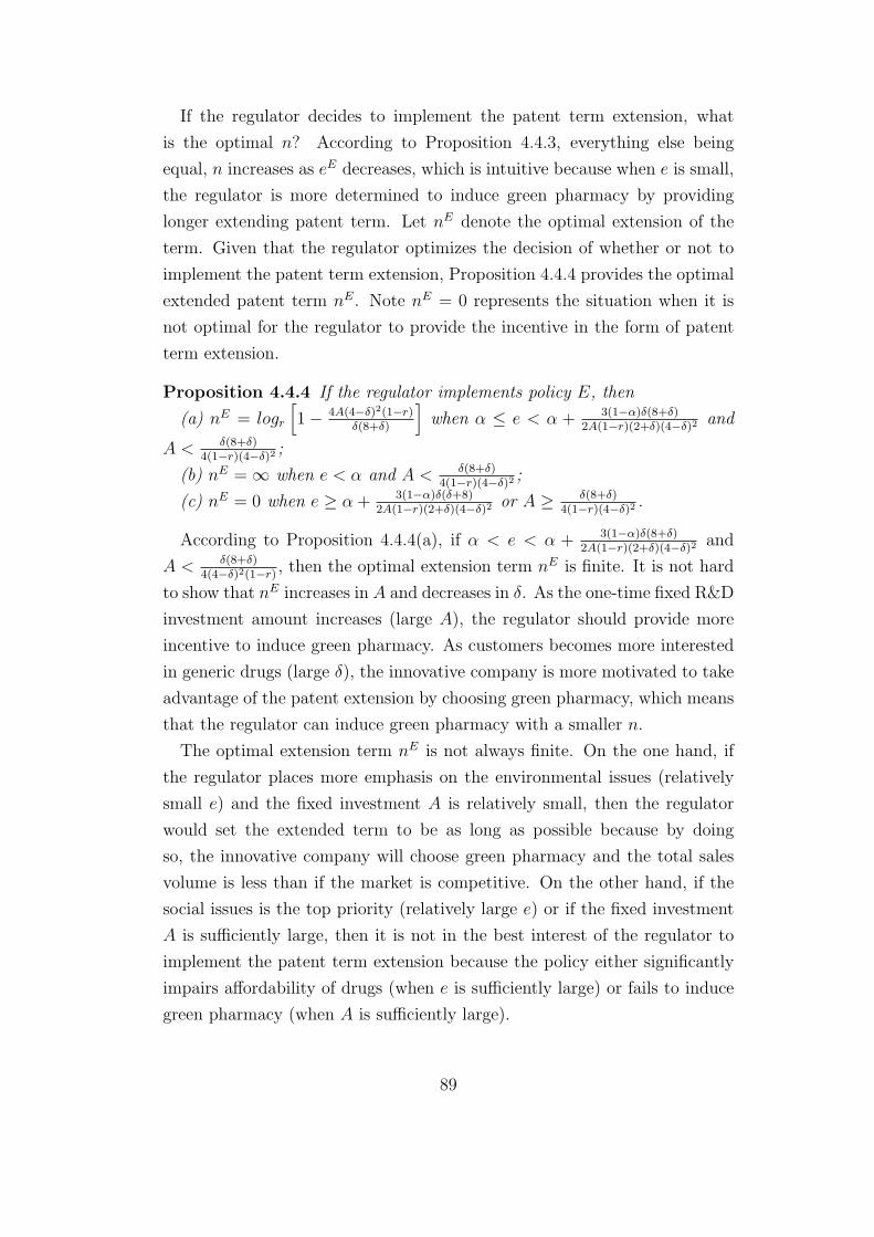
If the regulator decides to implement the patent term extension, what

is the optimal n? According to Proposition 4.4.3, everything else being

equal, n increases as eE decreases, which is intuitive because when e is small,

the regulator is more determined to induce green pharmacy by providing

longer extending patent term. Let nE denote the optimal extension of the

term. Given that the regulator optimizes the decision of whether or not to

implement the patent term extension, Proposition 4.4.4 provides the optimal

extended patent term nE. Note nE = 0 represents the situation when it is

not optimal for the regulator to provide the incentive in the form of patent

term extension.

Proposition 4.4.4 If the regulator implements policy E, then

(a) nE = logr

[1− 4A(4−δ)2(1−r)

δ(8+δ)

]when α ≤ e < α + 3(1−α)δ(8+δ)

2A(1−r)(2+δ)(4−δ)2and

A < δ(8+δ)4(1−r)(4−δ)2

;

(b) nE = ∞ when e < α and A < δ(8+δ)4(1−r)(4−δ)2

;

(c) nE = 0 when e ≥ α + 3(1−α)δ(δ+8)2A(1−r)(2+δ)(4−δ)2

or A ≥ δ(8+δ)4(1−r)(4−δ)2

.

According to Proposition 4.4.4(a), if α < e < α + 3(1−α)δ(8+δ)2A(1−r)(2+δ)(4−δ)2

and

A < δ(8+δ)4(4−δ)2(1−r)

, then the optimal extension term nE is finite. It is not hard

to show that nE increases in A and decreases in δ. As the one-time fixed R&D

investment amount increases (large A), the regulator should provide more

incentive to induce green pharmacy. As customers becomes more interested

in generic drugs (large δ), the innovative company is more motivated to take

advantage of the patent extension by choosing green pharmacy, which means

that the regulator can induce green pharmacy with a smaller n.

The optimal extension term nE is not always finite. On the one hand, if

the regulator places more emphasis on the environmental issues (relatively

small e) and the fixed investment A is relatively small, then the regulator

would set the extended term to be as long as possible because by doing

so, the innovative company will choose green pharmacy and the total sales

volume is less than if the market is competitive. On the other hand, if the

social issues is the top priority (relatively large e) or if the fixed investment

A is sufficiently large, then it is not in the best interest of the regulator to

implement the patent term extension because the policy either significantly

impairs affordability of drugs (when e is sufficiently large) or fails to induce

green pharmacy (when A is sufficiently large).

89

e1/151/131/11 1/9 1/7 1/5 1/3 1 3 5 7 9 11 13 15

A

0

0.05

0.1

0.15

0.2

0.25

0.3

0.35

0.4

(O,O)

(G0,F)+ (G

0,F)-

e1/151/131/11 1/9 1/7 1/5 1/3 1 3 5 7 9 11 13 15

δ

0

0.1

0.2

0.3

0.4

0.5

0.6

0.7

0.8

0.9

1

(O,O)

(G0,F)+ (G

0,F)-

e1/151/131/11 1/9 1/7 1/5 1/3 1 3 5 7 9 11 13 15

n

0

0.5

1

1.5

2

2.5

3

3.5

4

4.5

5

(O,O)

(G0,F)+ (G

0,F)-

Figure 4.3: Optimal Regulatory Policy: Policy N or Er = 0.8, and (L) n = 2, α = 0.5 and δ = 0.6; (M) A = 0.1, α = 0.5 and n = 2; (R)

A = 0.1, α = 0.5 and δ = 0.6.

4.5 The Role of Take-back Regulations

In the previous section, we demonstrated that the patent term extension

fails to encourage companies to invest in green pharmacy when A ≥ AE, no

matter how long the extended patent term n is. Therefore, in this section,

we consider another regulatory policy, take-back regulation, and evaluate its

impact on company strategy in Section 4.5.1. Intuitively, pharmaceutical

companies will not choose green pharmacy because the compliance cost

associated with the take-back regulation is usually independent of the choice

of green pharmacy. Thus, in Section 4.5.2, we compare the patent term

extension with and without the presence of the take-back regulation, and

discuss the optimal policy, optimal extended term and the resulting overall

social and environmental performance.

4.5.1 Pharmaceutical Take-back Regulations (Policy T )

As mentioned earlier, pharmaceutical take-back programs can help to reduce

environmental pollution by collecting and incinerating unwanted medicines.

However, it is unclear whether pharmaceutical take-back programs can in-

duce green pharmacy. One central issue in implementing this policy is

deciding how to pay for the cost of running the take-back program. In

the countries where the cost is financed by all participating pharmaceutical

companies, a common cost allocation scheme is based on the market size.

Thus, we model the problem as follows: In the presence of the take-back

regulation, each company has to pay the compliance cost ct per unit of sales.

90

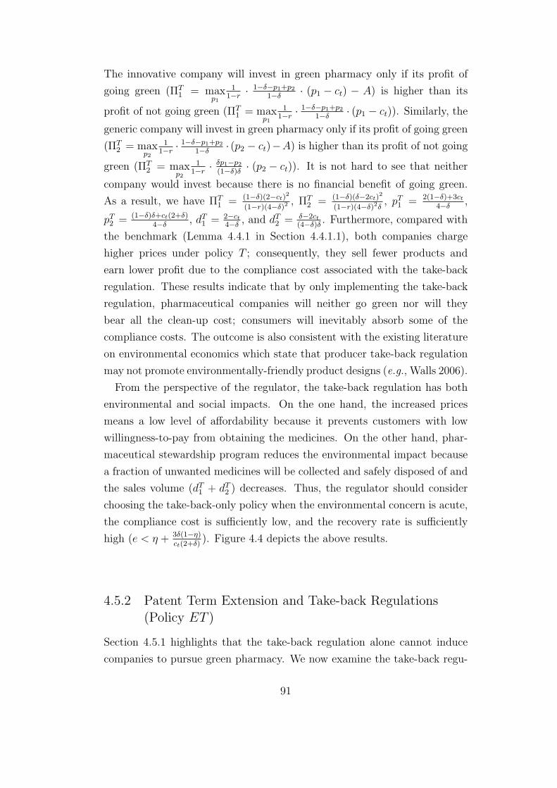
The innovative company will invest in green pharmacy only if its profit of

going green (ΠT1 = max

p1

11−r

· 1−δ−p1+p21−δ

· (p1 − ct) − A) is higher than its

profit of not going green (ΠT1 = max

p1

11−r

· 1−δ−p1+p21−δ

· (p1 − ct)). Similarly, the

generic company will invest in green pharmacy only if its profit of going green

(ΠT2 = max

p2

11−r

· 1−δ−p1+p21−δ

· (p2 − ct)−A) is higher than its profit of not going

green (ΠT2 = max

p2

11−r

· δp1−p2(1−δ)δ

· (p2 − ct)). It is not hard to see that neither

company would invest because there is no financial benefit of going green.

As a result, we have ΠT1 = (1−δ)(2−ct)

2

(1−r)(4−δ)2, ΠT

2 = (1−δ)(δ−2ct)2

(1−r)(4−δ)2δ, pT1 = 2(1−δ)+3ct

4−δ,

pT2 = (1−δ)δ+ct(2+δ)4−δ

, dT1 = 2−ct4−δ

, and dT2 = δ−2ct(4−δ)δ

. Furthermore, compared with

the benchmark (Lemma 4.4.1 in Section 4.4.1.1), both companies charge

higher prices under policy T ; consequently, they sell fewer products and

earn lower profit due to the compliance cost associated with the take-back

regulation. These results indicate that by only implementing the take-back

regulation, pharmaceutical companies will neither go green nor will they

bear all the clean-up cost; consumers will inevitably absorb some of the

compliance costs. The outcome is also consistent with the existing literature

on environmental economics which state that producer take-back regulation

may not promote environmentally-friendly product designs (e.g., Walls 2006).

From the perspective of the regulator, the take-back regulation has both

environmental and social impacts. On the one hand, the increased prices

means a low level of affordability because it prevents customers with low

willingness-to-pay from obtaining the medicines. On the other hand, phar-

maceutical stewardship program reduces the environmental impact because

a fraction of unwanted medicines will be collected and safely disposed of and

the sales volume (dT1 + dT2 ) decreases. Thus, the regulator should consider

choosing the take-back-only policy when the environmental concern is acute,

the compliance cost is sufficiently low, and the recovery rate is sufficiently

high (e < η + 3δ(1−η)ct(2+δ)

). Figure 4.4 depicts the above results.

4.5.2 Patent Term Extension and Take-back Regulations(Policy ET )

Section 4.5.1 highlights that the take-back regulation alone cannot induce

companies to pursue green pharmacy. We now examine the take-back regu-

91

e1/151/131/11 1/9 1/7 1/5 1/3 1 3 5 7 9 11 13 15

c t

0

0.02

0.04

0.06

0.08

0.1

0.12

0.14

0.16

0.18

0.2

T

N

e1/151/131/11 1/9 1/7 1/5 1/3 1 3 5 7 9 11 13 15

δ

0.1

0.2

0.3

0.4

0.5

0.6

0.7

0.8

0.9

1

T N

e1/151/131/11 1/9 1/7 1/5 1/3 1 3 5 7 9 11 13 15

η

0

0.1

0.2

0.3

0.4

0.5

0.6

0.7

0.8

0.9

1

T

N

Figure 4.4: Optimal Regulatory Policy: Policy N or T(L) δ = 0.6 and η = 0.5 ; (M) ct = 0.05 and η = 0.5; (R) ct = 0.05 and δ = 0.6.

lation in conjunction with the patent term extension? The research question

we ask is how would the optimal extended patent term be affected when both

policies are implemented?

To answer the above question, we first specify our models: the innovative

company decides whether to invest at time T0. If the innovative company

plans to invest, then it decides the monopoly price pm for the next n periods.

At time Tn, the generic company enters the market; the innovative company

decides p1 and the generic company decides p2 simultaneously. Therefore, the

profit of the innovative company is ΠET1 = max

pm,p1

1−rn

1−r· (1− pm) · (pm − ct) +

rn

1−r· 1−δ−p1+p2

1−δ· (p1 − ct) − A and the profit of generic company is ΠET

2 =

maxp2

rn

1−r· δp1−p2(1−δ)δ

· (p2 − ct). Note, in this case, the generic company can obtain

free access to the green pharmacy after Tn. If the innovative company decides

not to invest and, therefore, does not obtain patent term extension, then

the problem is essentially the same as that under policy T . Let AET =1−rn

1−r

[(1−ct)2

4− (2−ct)2(1−δ)

(4−δ)2

]. Similar to Lemma 4.4.2, we have

Lemma 4.5.1 In the presence of policy ET ,

(a) If A ≤ AET , then (G0, F ) is the equilibrium. ΠET1 = (2−ct)2(1−δ)rn

(4−δ)2(1−r)+

(1−ct)2(1−rn)4(1−r)

− A, ΠET2 = (1−δ)(δ−2ct)2rn

(4−δ)2(1−r). Moreover, pET

m = 1+ct2

dETm = 1−ct

2;

pETi = pTi and dET

i = dTi for i = 1, 2;

(b) If A > AET , then (O,O) is the equilibrium. ΠETi = ΠT

i , pETi = pTi , and

dETi = dTi for i = 1, 2.

(c) ΠETi ≤ ΠE

i for i = 1, 2.

It is not hard to show that, everything else being equal, the threshold of A

below which the innovative company will go green is lower under policy ET

92

than under policy E (AET ≤ AE) when ct ≤ δ2. This is because the decrease

in demand due to the compliance cost has a greater impact (in terms of profit

reduction) on the innovative company’s monopoly profit than on its profit

under the competition, which makes patent term extension less attractive.

In addition, as Lemma 4.5.1 states, in the presence of patent term extension,

both companies have less profit with the take-back regulation than without

it.

Nevertheless, policy ET can induce green pharmacy in cases where policy

T can never achieve it; also, policy ET can result in less negative impact

than policy E in some cases. Recall that the regulator aims to minimize the

following social and environmental impacts

e1Σ∞k=1r

k−1 (1− d1,k − d2,k) + ηte2Σ∞k=1r

k−1(αl1,kd1,k + αl2,kd1,k

)where t = 1 if the take-back regulation exists and t = 0 if otherwise;

d1,k, d2,k, l1,k, l2,k are defined in Section 4.4.2. Given the choice of implement-

ing both the patent term extension and the take-back regulation (policy ET )

or nothing (policy N), which one is the better strategy for the regulator? If

implementing both regulations, what is the optimal extended patent term?

Letting euET =(2+δ)(1−αη)[c2t(12−4δ+δ2)−2ct(8+δ2)+δ(8+δ)]

2A(4−δ)2(1−r)[3δ−ct(δ+2)]+3ct[c2t (12−4δ+δ2)−2ct(8+δ2)+δ(8+δ)], Proposi-

tion 4.5.2 specifies the optimal extended patent term nET .

Proposition 4.5.2 If the regulator implements policy ET , then

(a) nET = logr

[1− 4A(4−δ)2(1−r)

δ(8+δ)−2ct(8+δ2)+c2t (12−4δ+δ2)

]when αη ≤ e < max αη+

2(1−α)(2+δ)3δ

, αη + euET and A <δ(8+δ)−2ct(8+δ2)+c2t(12−4δ+δ2)

4(4−δ)2(1−r);

(b) nET = ∞ when e < αη and A <δ(8+δ)−2ct(8+δ2)+c2t(12−4δ+δ2)

4(1−r)(4−δ)2;

(c) nET = 0 when e ≥ maxαη + 2(1−α)(2+δ)

3δ, αη + euET

or A >

δ(8+δ)−2ct(8+δ2)+c2t(12−4δ+δ2)4(1−r)(4−δ)2

.

Similar to Proposition 4.4.4, Proposition 4.5.2 reveals that the optimal

extension term nET is finite when the environmental and social impacts are

to be balanced. By comparing Propositions 4.4.4 with 4.5.2, we have the

following corollary:

Corollary 4.5.3 nET ≥ nE when A <δ(8+δ)−2ct(8+δ2)+c2t(12−4δ+δ2)

4(1−r)(4−δ)2and α <

e < minα + 3(1−α)δ(8+δ)

2A(1−r)(2+δ)(4−δ)2,max

αη + 2(1−α)(2+δ)

3δ, αη + euET

.

93

e1/15 1/13 1/11 1/9 1/7 1/5 1/3 1 3 5 7 9 11 13 15

n*

0

2

4

6

8

10

12

14

16

E: n*

E: total impacts

ET: n*

ET: total impacts

δ

0.1 0.2 0.3 0.4 0.5 0.6 0.7 0.8 0.9 1

n*

0

1

2

3

4

5

6

7

E: n*

E: total impacts

ET: n*

ET: total impacts

ct

0 0.05 0.1 0.15 0.2 0.25

n*

0

1

2

3

4

5

6

E: n*

E: total impacts

ET: n*

ET: total impacts

Figure 4.5: Optimal Length of Patent Extension and Total Impacts underDifferent Policies

A = 0.1, α = 0.5, r = 0.8, η = 0.5. (L) ct = 0.05, δ = 0.6; (M) ct = 0.05, e = 2; (R)

δ = 0.6, e = 2.

According to Corollary 4.5.3 and Figure 4.5, the optimal patent term

extension is longer under policy ET than under policy E when nE and nET

are both finite, which means that more incentive must be provided to induce

green pharmacy with the take-back regulation than without such regulation.

This is because the innovative company’s monopoly profit is reduced from 14

to (1−c1)2

4per period due to the take-back regulation. Therefore, everything

else being equal, in order to encourage green pharmacy, the regulation has

to offer a longer patent term extension under policy ET .

In terms of the total impact, numerical results indicate that adding the

take-back regulation to the existing patent term extension could increase

or decrease the total impact, depending on the system parameters. First

of all, if the regulator aims to reduce the environmental impact (small e),

then in most cases, it is optimal for the regulator to adopt policy ET rather

than policy E because the take-back regulation helps to further reduce the

environmental impact. If the social impact is the main concern (large e),

then the regulator should only implement E rather than policy ET because

the take-back regulation increases the price of pharmaceutical products and

reduces the affordability of medicines. Second, when e is relatively small,

policy ET is more likely to outperform policy E as A increases. When A is

relatively large, companies have little motivation to invest in green pharmacy,

which means that policy ET (E) is essentially policy T (N). Thus, the

analysis in Section 4.5.1 follows. Third, adding the take-back regulation to

the existing patent term extension could decrease the total impact when the

94

compliance cost ct is relatively small. This is because policy ET with small

ct encourages safe disposal but merely changes the social impact. Fourth, it

is generally optimal for the regulator to adopt policy ET rather than policy

E when δ is sufficiently small or sufficiently large. When δ is sufficiently

small, the patent extension regulation can hardly induce green pharmacy

because the innovative company dominates the market. In fact, nE and nET

generally equal zero in such a case. However, the take-back regulation can

help achieve a lower environmental impact by collecting some of the unused

pharmaceutical products. When δ is sufficiently large, the regulator can

induce green pharmacy with small n because innovative company wants to

take advantage of the patent term extension in face of fierce competition. As

a result, the environmental impact is reduced while the social impact does not

significantly increase. Last, the total impact is typically lower under policy

ET than under policy E when η is relatively small, which is intuitive because

smaller η means a higher fraction of unused products can be safely disposed

of. Overall, similar to Section 4.5.1, we conclude that the environmental

impact is generally reduced because of the decreased sales and safe disposal;

however, the negative social impact is usually exaggerated due to the higher

price and the low level of affordability. In addition, policy ET excels policy

E when A is relatively large, when e, ct, and η are relatively small, and when

δ is either sufficiently small or sufficiently large.

4.6 Effects of Green Pharmacy on the Compliance

Cost

According to Section 4.5.1, the take-back regulation alone will not induce

green pharmacy because the program does not provide financial incentive to

the pharmaceutical company for engaging in green technology. This result

relies on the assumption that the compliance cost is independent of whether

a company adopts green pharmacy. In this section, we consider the case that

the compliance cost of the take-back regulation is related to the greenness of

the pharmaceutical products: companies without green pharmacy have the

base compliance cost ct per unit; however, companies with green pharmacy

have lower compliance cost α · ct per unit, where α is the degree of non-

greenness as we discussed before. This is a reasonable assumption because

95

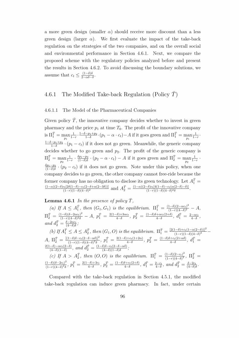
a more green design (smaller α) should receive more discount than a less

green design (larger α). We first evaluate the impact of the take-back

regulation on the strategies of the two companies, and on the overall social

and environmental performance in Section 4.6.1. Next, we compare the

proposed scheme with the regulatory policies analyzed before and present

the results in Section 4.6.2. To avoid discussing the boundary solutions, we

assume that ct ≤ (1−δ)δ2−αδ−δ

.

4.6.1 The Modified Take-back Regulation (Policy T )

4.6.1.1 The Model of the Pharmaceutical Companies

Given policy T , the innovative company decides whether to invest in green

pharmacy and the price p1 at time T0. The profit of the innovative company

is ΠT1 = max

p1

11−r

· 1−δ−p1+p21−δ

·(p1 − α · ct)−A if it goes green and ΠT1 = max

p1

11−r

·1−δ−p1+p2

1−δ· (p1 − ct) if it does not go green. Meanwhile, the generic company

decides whether to go green and p2. The profit of the generic company is

ΠT2 = max

p2

11−r

· δp1−p2(1−δ)δ

· (p2 − α · ct) − A if it goes green and ΠT2 = max

p2

11−r

·δp1−p2(1−δ)δ

· (p2 − ct) if it does not go green. Note under this policy, when one

company decides to go green, the other company cannot free-ride because the

former company has no obligation to disclose its green technology. Let AT1 =

(1−α)(2−δ)ct[2δ(1−δ)−ct(2−δ+α(2−3δ))](1−r)(1−δ)(4−δ)2

and AT2 = (1−α)(2−δ)ct[4(1−δ)−ct(α(2−δ)−δ)]

(1−r)(1−δ)(4−δ)2δ.

Lemma 4.6.1 In the presence of policy T ,

(a) If A ≤ AT1 , then (G1, G1) is the equilibrium. ΠT

1 = (1−δ)(2−αct)2

(1−r)(4−δ)2− A,

ΠT2 = (1−δ)(δ−2αct)

2

(1−r)(4−δ)2δ− A, pT1 = 2(1−δ)+3αct

4−δ, pT2 = (1−δ)δ+αct(2+δ)

4−δ, dT1 = 2−αct

4−δ,

and dT2 = δ−2αct(4−δ)δ

;

(b) If AT1 ≤ A ≤ AT

2 , then (G1, O) is the equilibrium. ΠT1 = [2(1−δ)+ct(1−α(2−δ))]2

(1−r)(1−δ)(4−δ)2−

A, ΠT2 = [(1−δ)δ−ct(2−δ−αδ)]2

(1−r)(1−δ)(4−δ)2δ, pT1 = 2(1−δ)+ct(1+2α)

4−δ, pT2 = (1−δ)δ+ct(2+αδ)

4−δ, dT1 =

2(1−δ)−αct(2−δ)(4−δ)(1−δ)

, and dT2 = (1−δ)δ−ct(2−δ−αδ)(4−δ)(1−δ)δ

;

(c) If A > AT2 , then (O,O) is the equilibrium. ΠT

1 = (1−δ)(2−ct)2

(1−r)(4−δ)2, ΠT

2 =

(1−δ)(δ−2ct)2

(1−r)(4−δ)2δ, pT1 = 2(1−δ)+3ct

4−δ, pT2 = (1−δ)δ+ct(2+δ)

4−δ, dT1 = 2−ct

4−δ, and dT2 = δ−2ct

(4−δ)δ.

Compared with the take-back regulation in Section 4.5.1, the modified

take-back regulation can induce green pharmacy. In fact, under certain

96

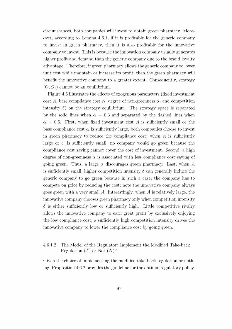
circumstances, both companies will invest to obtain green pharmacy. More-

over, according to Lemma 4.6.1, if it is profitable for the generic company

to invest in green pharmacy, then it is also profitable for the innovative

company to invest. This is because the innovation company usually generates

higher profit and demand than the generic company due to the brand loyalty

advantage. Therefore, if green pharmacy allows the generic company to lower

unit cost while maintain or increase its profit, then the green pharmacy will

benefit the innovative company to a greater extent. Consequently, strategy

(O,G1) cannot be an equilibrium.

Figure 4.6 illustrates the effects of exogenous parameters (fixed investment

cost A, base compliance cost ct, degree of non-greenness α, and competition

intensity δ) on the strategy equilibrium. The strategy space is separated

by the solid lines when α = 0.3 and separated by the dashed lines when

α = 0.5. First, when fixed investment cost A is sufficiently small or the

base compliance cost ct is sufficiently large, both companies choose to invest

in green pharmacy to reduce the compliance cost; when A is sufficiently

large or ct is sufficiently small, no company would go green because the

compliance cost saving cannot cover the cost of investment. Second, a high

degree of non-greenness α is associated with less compliance cost saving of

going green. Thus, a large α discourages green pharmacy. Last, when A

is sufficiently small, higher competition intensity δ can generally induce the

generic company to go green because in such a case, the company has to

compete on price by reducing the cost; note the innovative company always

goes green with a very small A. Interestingly, when A is relatively large, the

innovative company chooses green pharmacy only when competition intensity

δ is either sufficiently low or sufficiently high. Little competitive rivalry

allows the innovative company to earn great profit by exclusively enjoying

the low compliance cost; a sufficiently high competition intensity drives the

innovative company to lower the compliance cost by going green.

4.6.1.2 The Model of the Regulator: Implement the Modified Take-backRegulation (T ) or Not (N)?

Given the choice of implementing the modified take-back regulation or noth-

ing, Proposition 4.6.2 provides the guideline for the optimal regulatory policy.

97

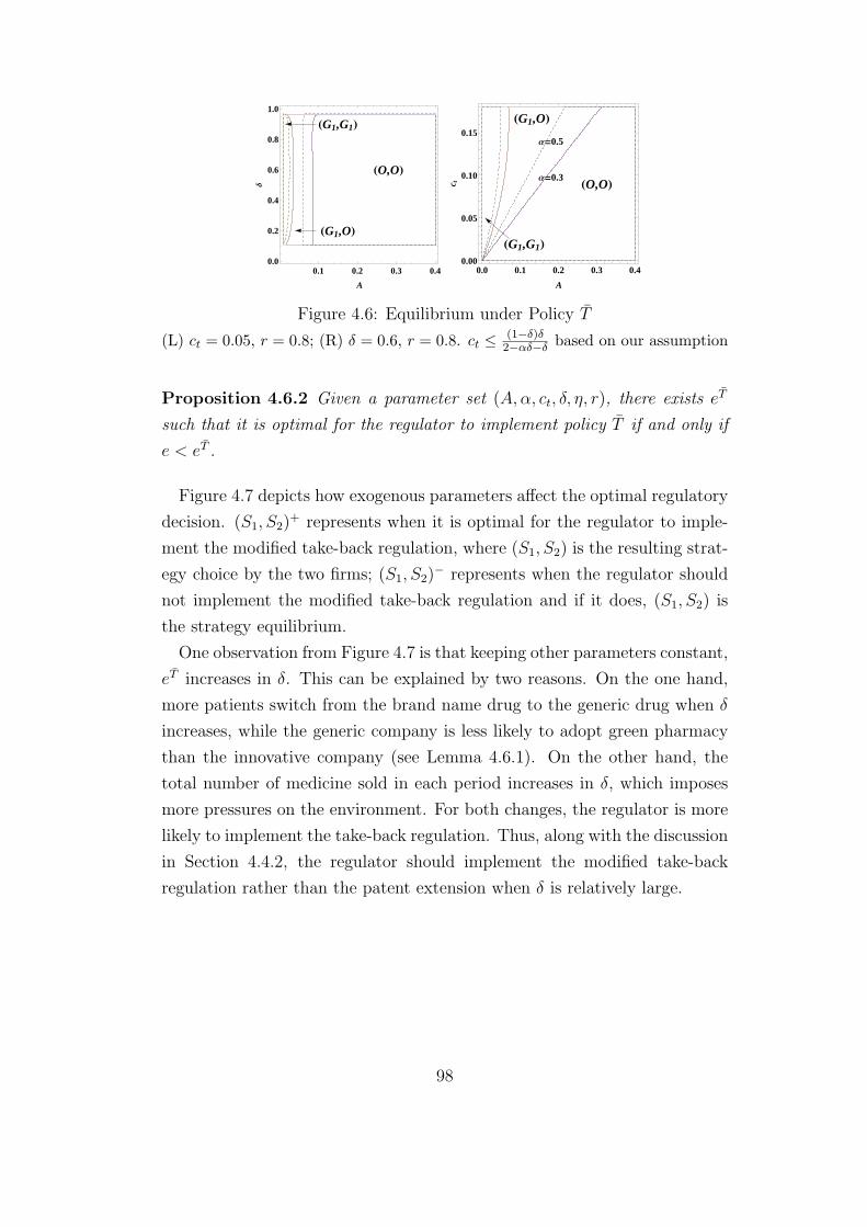
0.1 0.2 0.3 0.40.0

0.2

0.4

0.6

0.8

1.0

A

∆

HO,OL

HG1,OL

HG1,G1L

0.0 0.1 0.2 0.3 0.40.00

0.05

0.10

0.15

A

c t

Α=0.3

Α=0.5

HO,OL

HG1,OL

HG1,G1L

Figure 4.6: Equilibrium under Policy T

(L) ct = 0.05, r = 0.8; (R) δ = 0.6, r = 0.8. ct ≤ (1−δ)δ2−αδ−δ based on our assumption

Proposition 4.6.2 Given a parameter set (A,α, ct, δ, η, r), there exists eT

such that it is optimal for the regulator to implement policy T if and only if

e < eT .

Figure 4.7 depicts how exogenous parameters affect the optimal regulatory

decision. (S1, S2)+ represents when it is optimal for the regulator to imple-

ment the modified take-back regulation, where (S1, S2) is the resulting strat-

egy choice by the two firms; (S1, S2)− represents when the regulator should

not implement the modified take-back regulation and if it does, (S1, S2) is

the strategy equilibrium.

One observation from Figure 4.7 is that keeping other parameters constant,

eT increases in δ. This can be explained by two reasons. On the one hand,

more patients switch from the brand name drug to the generic drug when δ

increases, while the generic company is less likely to adopt green pharmacy

than the innovative company (see Lemma 4.6.1). On the other hand, the

total number of medicine sold in each period increases in δ, which imposes

more pressures on the environment. For both changes, the regulator is more

likely to implement the take-back regulation. Thus, along with the discussion

in Section 4.4.2, the regulator should implement the modified take-back

regulation rather than the patent extension when δ is relatively large.

98

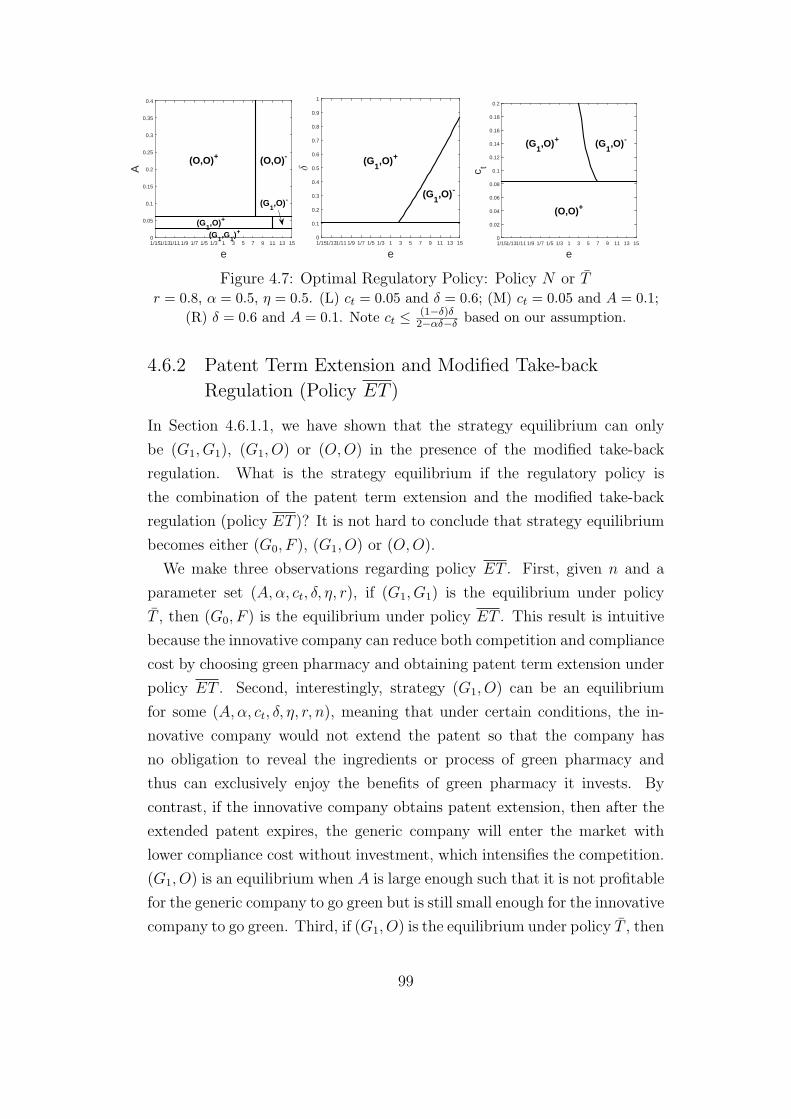
e1/151/131/11 1/9 1/7 1/5 1/3 1 3 5 7 9 11 13 15

A

0

0.05

0.1

0.15

0.2

0.25

0.3

0.35

0.4

(O,O)+ (O,O)-

(G1,O)+

(G1,O)-

(G1,G

1)+

e1/151/131/11 1/9 1/7 1/5 1/3 1 3 5 7 9 11 13 15

δ

0

0.1

0.2

0.3

0.4

0.5

0.6

0.7

0.8

0.9

1

(G1,O)+

(G1,O)-

e1/151/131/11 1/9 1/7 1/5 1/3 1 3 5 7 9 11 13 15

c t

0

0.02

0.04

0.06

0.08

0.1

0.12

0.14

0.16

0.18

0.2

(O,O)+

(G1,O)+ (G

1,O)-

Figure 4.7: Optimal Regulatory Policy: Policy N or Tr = 0.8, α = 0.5, η = 0.5. (L) ct = 0.05 and δ = 0.6; (M) ct = 0.05 and A = 0.1;

(R) δ = 0.6 and A = 0.1. Note ct ≤ (1−δ)δ2−αδ−δ based on our assumption.

4.6.2 Patent Term Extension and Modified Take-back

Regulation (Policy ET )

In Section 4.6.1.1, we have shown that the strategy equilibrium can only

be (G1, G1), (G1, O) or (O,O) in the presence of the modified take-back

regulation. What is the strategy equilibrium if the regulatory policy is

the combination of the patent term extension and the modified take-back

regulation (policy ET )? It is not hard to conclude that strategy equilibrium

becomes either (G0, F ), (G1, O) or (O,O).

We make three observations regarding policy ET . First, given n and a

parameter set (A,α, ct, δ, η, r), if (G1, G1) is the equilibrium under policy

T , then (G0, F ) is the equilibrium under policy ET . This result is intuitive

because the innovative company can reduce both competition and compliance

cost by choosing green pharmacy and obtaining patent term extension under

policy ET . Second, interestingly, strategy (G1, O) can be an equilibrium

for some (A,α, ct, δ, η, r, n), meaning that under certain conditions, the in-

novative company would not extend the patent so that the company has

no obligation to reveal the ingredients or process of green pharmacy and

thus can exclusively enjoy the benefits of green pharmacy it invests. By

contrast, if the innovative company obtains patent extension, then after the

extended patent expires, the generic company will enter the market with

lower compliance cost without investment, which intensifies the competition.

(G1, O) is an equilibrium when A is large enough such that it is not profitable

for the generic company to go green but is still small enough for the innovative

company to go green. Third, if (G1, O) is the equilibrium under policy T , then

99

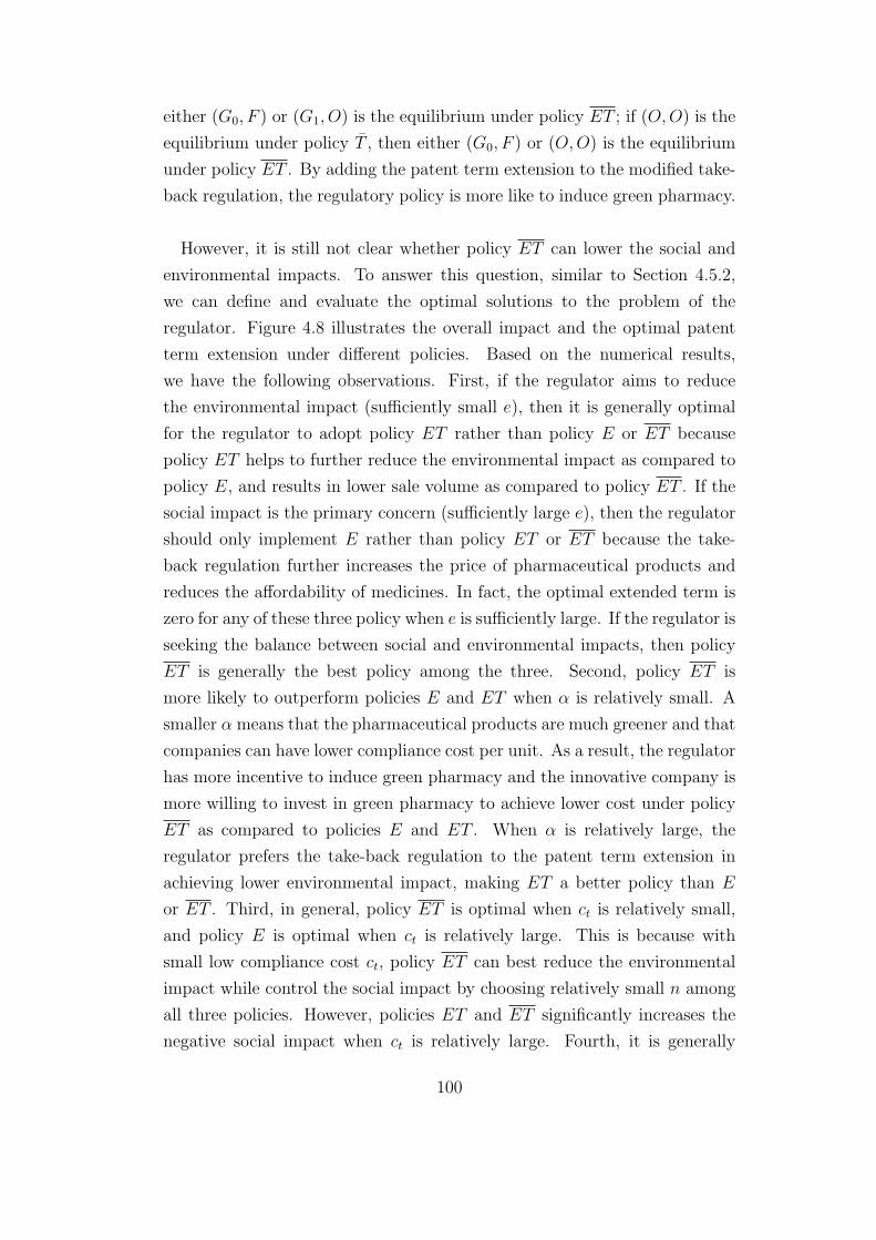
either (G0, F ) or (G1, O) is the equilibrium under policy ET ; if (O,O) is the

equilibrium under policy T , then either (G0, F ) or (O,O) is the equilibrium

under policy ET . By adding the patent term extension to the modified take-

back regulation, the regulatory policy is more like to induce green pharmacy.

However, it is still not clear whether policy ET can lower the social and

environmental impacts. To answer this question, similar to Section 4.5.2,

we can define and evaluate the optimal solutions to the problem of the

regulator. Figure 4.8 illustrates the overall impact and the optimal patent

term extension under different policies. Based on the numerical results,

we have the following observations. First, if the regulator aims to reduce

the environmental impact (sufficiently small e), then it is generally optimal

for the regulator to adopt policy ET rather than policy E or ET because

policy ET helps to further reduce the environmental impact as compared to

policy E, and results in lower sale volume as compared to policy ET . If the

social impact is the primary concern (sufficiently large e), then the regulator

should only implement E rather than policy ET or ET because the take-

back regulation further increases the price of pharmaceutical products and

reduces the affordability of medicines. In fact, the optimal extended term is

zero for any of these three policy when e is sufficiently large. If the regulator is

seeking the balance between social and environmental impacts, then policy

ET is generally the best policy among the three. Second, policy ET is

more likely to outperform policies E and ET when α is relatively small. A

smaller α means that the pharmaceutical products are much greener and that

companies can have lower compliance cost per unit. As a result, the regulator

has more incentive to induce green pharmacy and the innovative company is

more willing to invest in green pharmacy to achieve lower cost under policy

ET as compared to policies E and ET . When α is relatively large, the

regulator prefers the take-back regulation to the patent term extension in

achieving lower environmental impact, making ET a better policy than E

or ET . Third, in general, policy ET is optimal when ct is relatively small,

and policy E is optimal when ct is relatively large. This is because with

small low compliance cost ct, policy ET can best reduce the environmental

impact while control the social impact by choosing relatively small n among

all three policies. However, policies ET and ET significantly increases the

negative social impact when ct is relatively large. Fourth, it is generally

100

optimal for the regulator to adopt policy ET , especially when δ is small.

Similar to the analysis in Section 4.5.2, when δ is sufficiently small, on the one

hand, unless n is sufficiently large, the patent extension regulation can hardly

induce green pharmacy because the brand name product already dominates

the market; on the other hand, the take-back regulation can help achieve a

lower environmental impact by having some of the unused pharmaceutical

products safely disposed. Thus, the regulator can collect unused products

and induce green pharmacy with smaller n under policy ET than under

other policies. Last, the total impact is generally lower under policy ET

than under policy E or ET when η is relatively small because a relatively

high proportion of unused products can be safely disposed of under policy

ET with small η. Overall, policy ET is more favorable than policies E and

ET , especially when α, ct, δ, and η are relatively small. However, policy ET

can excel policies E and ET when e is relatively small and α is relatively

large; policy E can excel polices ET and ET when e and ct are relatively

large.

4.7 Conclusion

Unused pharmaceuticals are disposed of unsafely in increasingly large vol-

umes every year. The eco-toxicity arising from unused pharmaceuticals

has drawn considerable attention of policy makers, such as the EPA in the

U.S and EEA in Europe, who are now advocating the concept of “green

pharmacy”. The key element of green pharmacy is “benign by design”, which

aims to eliminate or reduce the use and generation of hazardous substances.

However, the major obstacles to the achievement of green pharmacy are

high R&D expenses and the lack of incentives and regulations. One pos-

sible incentive, as proposed by EEA, is to offer a patent term extension

to pharmaceutical companies that formulate greener drugs. Such incen-

tive can encourage both the development of degradable green drugs and

technical information disclosure. Yet, it is still unclear how effective the

pharmaceutical patent term extension is in inducing green pharmacy and

the implication of patent term extension for the social and environmental

impacts. Toward that end, we consider an innovative company who collects

monopoly profits for its patented medicine and faces competition from a

101

generic rival after the patent expires. Each company can achieve green

pharmacy by investing a fixed amount. However, the generic rival can acquire

green pharmacy, free of charge, after the expiry of the extended patent that

is granted to the innovative company for its development of green pharmacy.

Both the social impact (the affordability of pharmaceutical products) and

environmental impact (contamination of unwanted pharmaceuticals in the

environment) are considered by the regulator when determining the optimal

extended patent term. We demonstrate that in the presence of the patent

term extension, the innovative company will invest in green pharmacy when

the fixed investment cost is low, the extended term of the patent is long

and the competition intensity is high. However, patent term extension can

result in a lack of affordability. As a result, the regulator should implement

the patent extension only with a sufficiently high level of environmental

concern. Specifically, the optimal extended term is finite when the regulator

is seeking the balance of controlling both social and environmental impacts;

the extended term should increase as the fixed investment cost increases or

the market competition becomes less competitive.

Pharmaceutical stewardship program is another possible approach to pro-

moting green pharmacy. However, pharmaceutical companies will not choose

green pharmacy in the presence of the take-back regulation because the unit

compliance cost is typically independent of the choice of green pharmacy;

worse still, companies will raise the price so that the consumers partly pay the

cost incurred due to the pharmaceutical stewardship program. Nevertheless,

we conclude that implementing both the take-back regulation and the patent

term extension dominates the single policy of the patent term extension

when the compliance cost is relatively small, the fixed investment cost and

the collection rate are relatively large, the competition is either nominal

or sufficiently intensive, and the environmental issue is relatively urgent.

In addition, we propose a modified take-back regulation such that the unit

compliance cost is lower for companies with green pharmacy than without

green pharmacy. Such regulation can encourage both companies to invest in

green pharmacy and is better than the patent extension when the competition

intensity is relatively high. Numerical results indicate that the modified take-

back regulation is generally superior to the traditional take-back regulation

when the regulator considers adding the take-back regulation to the patent

term extension. An interesting observation is that the innovative company

102

would sometimes go green without requesting patent extension under the

modified joint policy. The reason is that the generic company cannot take

a free-ride after the patent expires, which helps the innovative company to

lessen the competition from the generics. However, a single policy of patent

term extension can still outperform a combined policy when the needs of

pharmaceuticals are compelling or when the compliance cost is relatively

large.

We note that our results are based in part on the assumption that a

company can obtain green pharmacy either by its R&D investment or by

waiting for the technical disclosure of its competitor after patent expires.

Nevertheless, we also consider, as a modeling extension, the possibility that

it takes sufficiently short time for the generic company to duplicate an

unpatented green technology without enabling disclosure. For this extension,

we find that the previous analysis for policies N and E remains unchanged.

However, this extension can change the equilibria under policy T or T .

Assuming that when the innovative or generic company invests in green

technology, the probability that the green technology is hard to duplicate

is p, and the probability that it is easy to duplicate is 1 − p. We consider

p < 1 because p = 1 represents the case we have already discussed before.

We find that, in general, our qualitative results and insights continue to

apply. However, compared with Lemma 4.6.1, (G1, G1) is less likely to be

the equilibrium while (O,O) is more likely to be the equilibrium. This is

because companies are hesitant to invest in green pharmacy when facing

a potential imitation risk by its competitor and a potential opportunity of

free-ride. Interestingly, when p is sufficiently small, the equilibria are not

unique under certain circumstance: the fact that (G1, O) and (O,G1) are

both equilibria indicates that it is profitable for a company to take a free

ride if its competitor invests in green pharmacy while it is still profitable

to invest if its competitor does not. From the perspective of the regulator,

implementing policy T or T can be more effective with p < 1 than p = 1

because the possibility of easy duplication of green pharmacy could lead to

the reduction in environmental impact.

In closing, we acknowledge the following limitations of our model. First,

it implicitly assumes that the GHG emissions associated with the collection

and disposal of unused and wasted medicine are nominal, and the APIs

introduced to sewage as a result of excretion are negligible. In fact, these

103

impacts can sometimes be remarkable. For example, Bound and Voulvoulis

(2005) estimated that a total of 34% of metabolic products was excreted

in active forms though “active” may not necessarily be interpreted as “eco-

toxic”. In principle, the relaxation of these two assumptions will lead to

a greater emphasis by the regulator on the promotion of green pharmacy

because green pharmacy reduces the requirement for collection and lowers

the risk of eco-toxicity caused by excretion or bathing. Second, the demand

of pharmaceuticals is assumed to be price-sensitive, which generally holds for

over-the-counter products. For prescribed medicines, recommendations by

the doctors and the third-party payment make the price elasticity of demand

relatively small, which can favor the small innovations (Ganuza et al. 2009).

104

Table 4.1: Model Notation

Decision Variables of the Pharmaceutical Companies

pm, dm the monopoly price and demand of brand name drugs,respectively, before the patent expires

p1(p2), d1(d2) the price and demand of brand name drugs (generic drugs),respectively, after the patent expires

S1(S2) the strategies of the innovative (generic) company, whereS1 ∈ G0, G1, O and S2 ∈ F,G1, OG0: the strategy of investing green pharmacy and obtainingpatent extension

G1: the strategy of investing green pharmacy but notgaining patent extension

O: the strategy of not going green

F : the strategy of going green for free after patent expires

Decision Variables of the Regulator

Sr the environmental policy implemented by the regulator,where Sr ∈ N,E, T,ETPolicy N : no environmental policy

Policy E: patent term extension

Policy T : take-back regulation

Policy ET : patent term extension and take-back regulation

n the length of extended term

Parameters

α degree of non-greenness

A one-time fixed R&D investment in green pharmacy

ct base compliance cost of the take-back regulation per unit

δ valuation factor of generic drugs

e1 social impact of unaffordable medicine per person per period(in monetary terms)

e2 environmental impact per unit per period (in monetary terms)

e impact ratio. e = e1e2

η proportion of unwanted drugs that are unsafely disposed(without being taken back)

r discount factor

T0 the time when the original patent expires

105

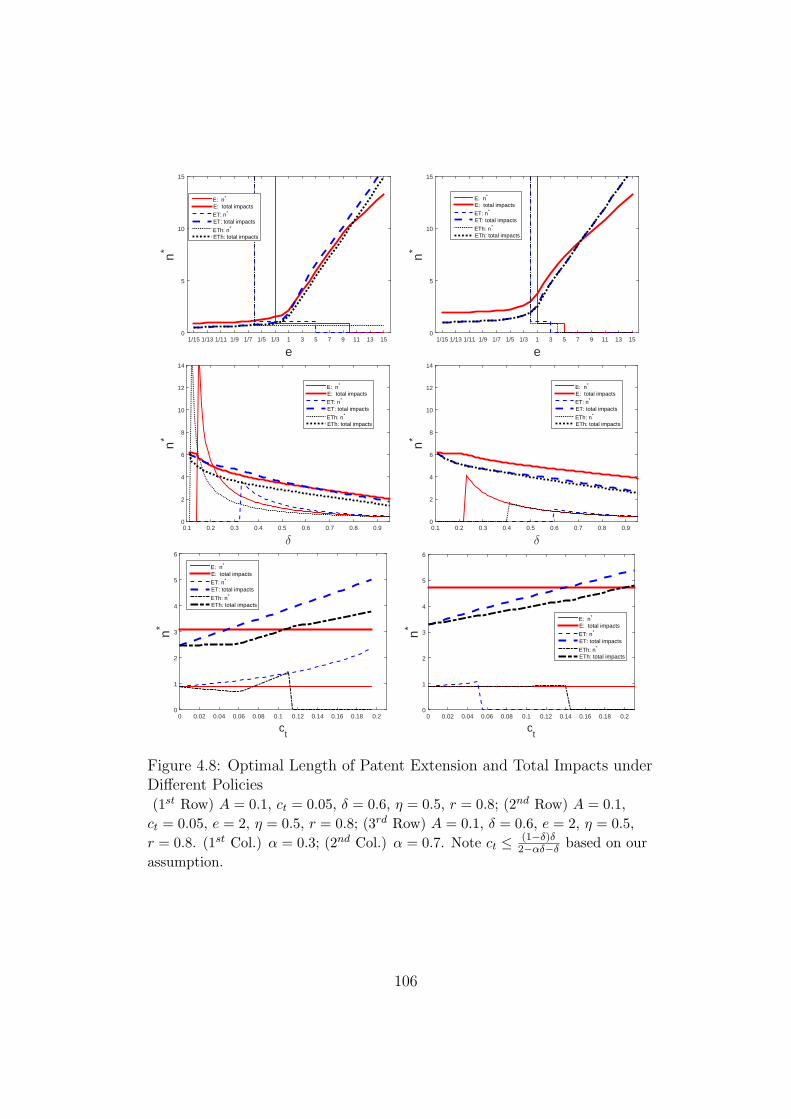
e1/15 1/13 1/11 1/9 1/7 1/5 1/3 1 3 5 7 9 11 13 15

n*

0

5

10

15

E: n*

E: total impacts

ET: n*

ET: total impacts

ETh: n*

ETh: total impacts

e1/15 1/13 1/11 1/9 1/7 1/5 1/3 1 3 5 7 9 11 13 15

n*

0

5

10

15

E: n*

E: total impacts

ET: n*

ET: total impacts

ETh: n*

ETh: total impacts

δ

0.1 0.2 0.3 0.4 0.5 0.6 0.7 0.8 0.9

n*

0

2

4

6

8

10

12

14

E: n*

E: total impacts

ET: n*

ET: total impacts

ETh: n*

ETh: total impacts

δ

0.1 0.2 0.3 0.4 0.5 0.6 0.7 0.8 0.9

n*

0

2

4

6

8

10

12

14

E: n*

E: total impacts

ET: n*

ET: total impacts

ETh: n*

ETh: total impacts

ct

0 0.02 0.04 0.06 0.08 0.1 0.12 0.14 0.16 0.18 0.2

n*

0

1

2

3

4

5

6

E: n*

E: total impacts

ET: n*

ET: total impacts

ETh: n*

ETh: total impacts

ct

0 0.02 0.04 0.06 0.08 0.1 0.12 0.14 0.16 0.18 0.2

n*

0

1

2

3

4

5

6

E: n*

E: total impacts

ET: n*

ET: total impacts

ETh: n*

ETh: total impacts

Figure 4.8: Optimal Length of Patent Extension and Total Impacts underDifferent Policies(1st Row) A = 0.1, ct = 0.05, δ = 0.6, η = 0.5, r = 0.8; (2nd Row) A = 0.1,

ct = 0.05, e = 2, η = 0.5, r = 0.8; (3rd Row) A = 0.1, δ = 0.6, e = 2, η = 0.5,

r = 0.8. (1st Col.) α = 0.3; (2nd Col.) α = 0.7. Note ct ≤ (1−δ)δ2−αδ−δ based on our

assumption.

106

CHAPTER 5

CONCLUSION

“There is no Plan B because we do not have a Planet B.”

– Ban Ki-moon.

In 2014, U.S. EPA published the third edition of Climate Change Indicators

in the United States. According to the report, average U.S. and global

temperatures are rising, snow and rainfall patterns are changing, extreme

weather and climate events are increasing, ragweed pollen season and growing

season for crops are lengthening, and the oceans are becoming more acidic.

Scientific evidence shows that many of these climate changes are linked to the

increase in greenhouse gases emissions as a result of human activities (U.S.

EPA 2014). To reduce the greenhouse gasses emissions, a large number of

research endeavors have been made in the past several decades; however,

more efforts are needed to help us live sustainable lives and save our planet.

Eco-friendly design has been one of the key topics studied in sustainable

operations management. Growing research attention has been shifting from

an end-of-pipe-control approach to a benign-by-design approach (Angell and

Klassen 1999). Eco-friendly design is motivated by the potential economic

benefits, stringent environmental legislation, and growing public awareness,

among others. In the remanufacturing industry, Design for the Environment

(DfE) has proven to be a key to the success of product recovery operations.

DfE helps bring full potential of product recovery into play in the context

of different firm or market structures. DfE is also equally applied to the

products that have little end-of-life value. It enables companies to use

fewer harmful components during manufacturing and to minimize pollutant

releases to the environment after disposal.

This dissertation discusses the mechanisms to promote DfE and the conse-

quences of implementing DfE, as illustrated in Figure 5.1. DfE is not always

107

DfE

Coordination

Scheme

Regulatory

Policy

Pricing

Planet

PeopleProfit

Figure 5.1: Research Focus of This Dissertation

a natural choice by the producers and sometimes external incentives or regu-

lations are needed to induce DfE. Two regulatory policies are analyzed in the

setting of the pharmaceutical industry: patent extension and take-back reg-

ulation. Another approach to achieving DfE is through inter-organizational

coordination. This dissertation examines the effectiveness of imposing single-

parameter schemes (transfer price or fixed lump sum transfer) and two-part

tariff to pursue DfE.

DfE facilitates product end-of-life recovery and can reduce adverse envi-

ronmental impacts. However, DfE can also increase the production cost and

result in higher product prices. Understanding the impact of design decisions

on profit, people, and planet is critical in analyzing DfE. Therefore, in this

dissertation, a firm or a division maximizes its profit by deciding product

design and prices; demand can be characterized by consumer’s vertical dif-

ferentiation and price; and decisions made by firms and consumers influence

the environmental impact.

This dissertation makes the following contributions: It extends the analysis

of take-back regulation to pharmaceuticals and makes the first attempt to val-

idate the proposal of implementing patent extension in achieving DfE. It also

extends supply chain coordination studies by incorporating DfE decisions. In

addition, the study develops guidelines for optimal pricing to companies that

embrace the idea of DfE. To probe deeper into the consequences of DfE, this

108

dissertation defines and evaluates different stakeholders and environmental

measures, and it relates environmental stewardship to other outcomes such

as profit, revenue and social welfare.

There are still many open questions regarding the promotion, implemen-

tation, and consequences of DfE. The work presented in this dissertation can

be extended in several ways.

One line of future research might be to study DfE in the context of

service operations. The current DfE tools are mainly applied to physical

merchandises, such as heavy-duty and off-road equipment, motor vehicle

parts, IT products and medical devices. However, a recent transition is from

selling physical products to offering a service-based package (Corbett and

Klassen 2006). Researchers have demonstrated that the adoption of green

practices is related to better firm performance in some service industries (e.g.,

Goodman 2000, Kassinis and Soteriou 2003). Unfortunately, little attention

has been paid to the DfE approach for service systems and the examination of

potential economic and environmental benefits of DfE in the service industry.

Another direction for future research is to develop and evaluate a more

comprehensive DfE that deals with the recovery of heterogeneous end-of-life

products of the same generation and the upgradeability of a product over

multiple generations. Optimizing the design of a product portfolio can offer

more practical applications than an all-in-one approach; however, considering

a product portfolio design can potentially increase the complexity of the

target system. Thus, a comprehensive DfE analysis along with large-scale

optimization methods, such as a hierarchical approach or a decomposition

approach, need to be developed in the future.

Additionally, data-driven analysis that encodes system parameters is an-

other potential to advance the study of DfE. Encouraged by emerging big

data applications, researchers can build more sophisticated models in which

dynamics and uncertainty embedded in DfE can be addressed in a joint

manner. For example, the demand or the willingness-to-pay for an eco-

friendly product can be estimated using a data-driven tool before the product

is launched or reintroduced. Another application of data-driven analysis

techniques is DEA-based energy and environmental efficiency measurement

and monitoring (Zhou et al. 2008). The DEA models and its extensions can

be employed to analyze the environmental performance of DfE.

109

The topic of DfE in the pharmaceutical industry is relatively new in the

field of operations management. Many other operational questions related

to pharmaceutical stewardship remain unanswered. For example, what is

the best approach to collect unwanted medical products: the mail-back

program, the permanent disposal program, or the periodically scheduled

collection program? The method of collection may significantly influence the

participation rate, the ease of operations, cost, and greenhouse gas emissions.

Another question is how to allocate cost and resources (e.g., reverse logistics

networks) when collecting unused and expired medical products? The collec-

tion and disposal costs are sometimes funded in part by manufacturers based

on prior year’s sales volumes (e.g., in France and Canada). However, such

an allocation mechanism does not consider the synergies inherent in resource

sharing among participating companies. Thus, it is critical to develop a cost

allocation mechanism that not only induces resource sharing in the collective

system, but also maximizes cost efficiency or increases return rate.

110

APPENDIX A

APPENDIX FOR CHAPTER 2

APPENDIX A.1 PROOF OF PROPOSITIONS

Proof of Proposition 2.3.1. Part (i) follows directly from the constraint

that the manufacturer cannot remanufacture more products than returned

products as follows: dor+dnr ≤ dnn+dnr ⇒ dor ≤ dnn. Thus, dor > 0 implies

that dnn > 0.

Part (ii) is by contradiction. From Table 2.1, dnr > 0 ⇒ ∃ θ1 such that

Snr (θ1) ≥ Snn (θ1) ⇔ θ1 ≤ p2−prα−δr

and Snr (θ1) ≥ Sor (θ1) ⇔ θ1 ≥ p1−s. Thus,

the existence of θ1 requires that p1−s ≤ p2−prα−δr

. Note p1−s = p2−prα−δr

⇒ dnr = 0.

Thus, dnr > 0 requires that p1 − s < p2−prα−δr

. Similarly, don > 0 ⇒ ∃ θ2 such

that Son (θ2) ≥ Snn (θ2) ⇔ θ2 ≤ p1 − s and Son (θ2) ≥ Sor (θ2) ⇔ θ2 ≥ p2−prα−δr

.

Thus, the existence of θ2 requires thatp2−prα−δr

≤ p1−s, which is a contradiction.

To prove part (iii), we use Table 2.2(a) because dnr = dor = 0, by

assumption. Assume dnn > 0. If don = 0, then dnu = 0 only whenp2α−δ

− p11+δ

≤ 0; if dnu = 0, then don = 0 only when p1 − p2α

≤ 0. Therefore,

after some algebra, we must have αp1 ≤ p2 ≤ α−δ1+δ

p1, which is impossible if

p1 = 0 or p2 = 0 because α > α−δ1+δ

> 0. Proof of Proposition 2.3.2. Part (i). In both cases, customers either

buy the only offered product or do not purchase. We first consider when the

offered product is available only in the second period. The object function can

be written as Π00010 = maxp2 (p2 − c0) · don subject to don > 0, p2 ≥ 0. Since

dnr = dor = 0, s = 0 and don = 1− p2α. It is easy to show that p∗2 =

α+c02

and

Π∗00010 = (α−c0)

2

4αwhen c0 < α and Π∗

00010 = 0 (no production) when c0 ≥ α.

Similarly, when the offered new product is available only in the first period.

It is straightforward to show that p∗1 = 1+δ+c02

and Π∗00100 = (1+δ−c0)

2

4(1+δ)when

c0 < 1 + δ and Π∗00100 = 0 (no production) when c0 ≥ 1 + δ.

When c0 < α, we must have c0 < 1+δ because α < 1+δ. Thus, Π∗00100 > 0

whenever Π∗00010 > 0. Moreover, Π∗

00010 = (α−c0)2

4α> Π∗

00100 = (1+δ−c0)2

4(1+δ)only

111

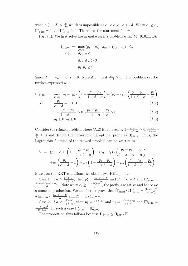
when α (1 + δ) > c20, which is impossible as c0 < α, c0 < 1+ δ. When c0 ≥ α,

Π∗00010 = 0 and Π∗

00100 ≥ 0. Therefore, the statement follows.

Part (ii). We first solve the manufacturer’s problem when M=(0,0,1,1,0):

Π01010 = maxp1,p2

(p1 − c0) · dnu + (p2 − c0) · dons.t dnn = 0

dnu, don > 0

p1, p2 ≥ 0

Since dnr = dor = 0, s = 0. Note dnn = 0 if p2α−δ

≥ 1. The problem can be

further expressed as

Π00110 = maxp1,p2

(p1 − c0) ·(1− p1 − p2

1 + δ − α

)+ (p2 − c0) ·

(p1 − p2

1 + δ − α− p2

α

)s.t.

p2α− δ

− 1 ≥ 0 (A.1)

1− p1 − p21 + δ − α

> 0,p1 − p2

1 + δ − α− p2

α> 0 (A.2)

p1 ≥ 0, p2 ≥ 0 (A.3)

Consider the relaxed problem where (A.2) is replaced by 1− p1−p21+δ−α

≥ 0, p1−p21+δ−α

−p2α

≥ 0 and denote the corresponding optimal profit as Π∗00110. Thus, the

Lagrangian function of the relaxed problem can be written as

L = (p1 − c0) ·(1− p1 − p2

1 + δ − α

)+ (p2 − c0) ·

(p1 − p2

1 + δ − α− p2

α

)+µ1

(p2

α− δ− 1

)+ µ2

(1− p1 − p2

1 + δ − α

)+ µ3

(p1 − p2

1 + δ − α− p2

α

)Based on the KKT conditions, we obtain two KKT points:

Case 1: if a ≥ 2δ(1+δ)1+δ−c0

, then p∗1 = (α−δ)(1+δ)α

and p∗2 = α − δ and Π∗00110 =

δ[(α−δ)(1+δ)−αc0]α2 . Note when c0 ≥ (α−δ)(1+δ)

α, the profit is negative and hence we

assume no production. We can further prove that Π∗00110 ≤ Π∗

00100 =(1+δ−c0)

2

4(1+δ)

when c0 <(α−δ)(1+δ)

αand 2δ < α < 1 + δ.

Case 2: if a < 2δ(1+δ)1+δ−c0

, then p∗1 = 1+δ+c02

and p∗2 = α(1+δ+c0)2(1+δ)

and Π∗00110 =

(1+δ−c0)2

4(1+δ). In such a case Π∗

00110 = Π∗00100.

The proposition thus follows because Π∗00110 ≤ Π∗

00110.

112

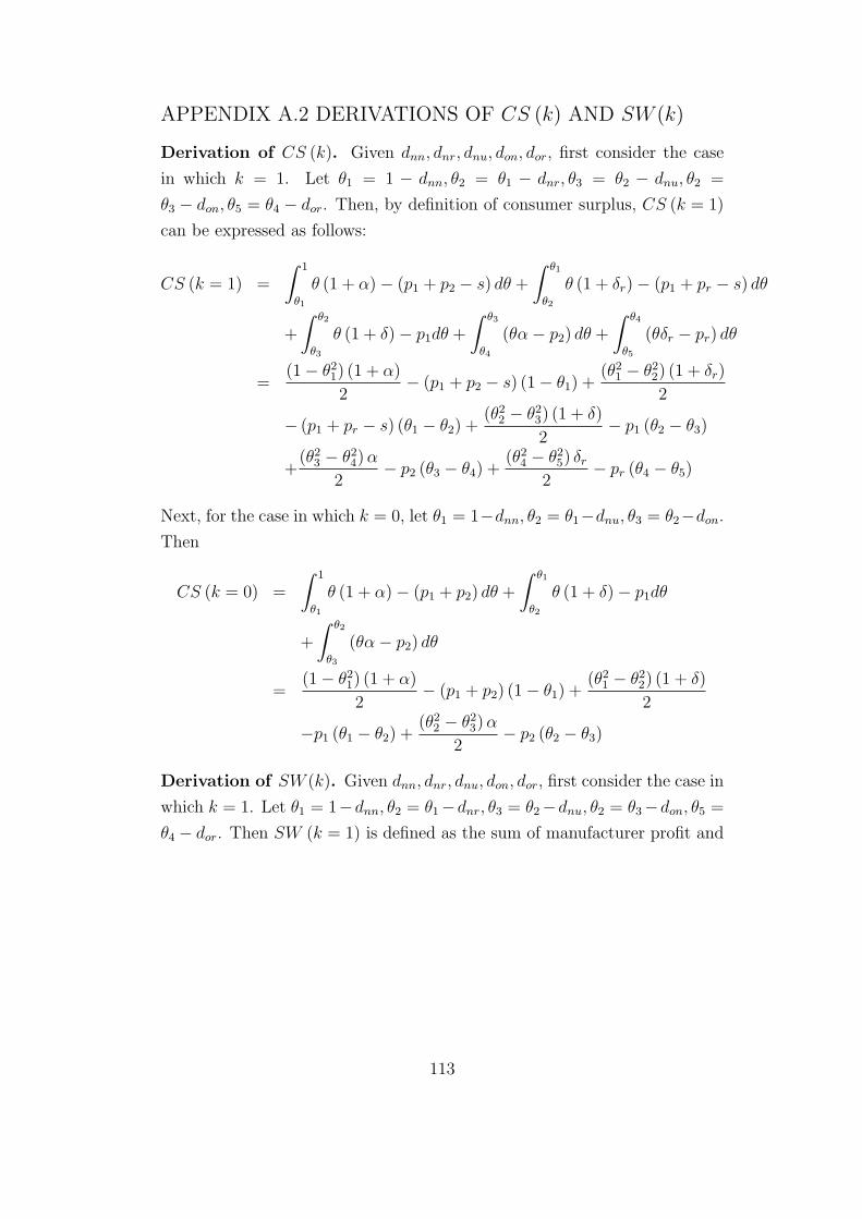
APPENDIX A.2 DERIVATIONS OF CS (k) AND SW (k)

Derivation of CS (k). Given dnn, dnr, dnu, don, dor, first consider the case

in which k = 1. Let θ1 = 1 − dnn, θ2 = θ1 − dnr, θ3 = θ2 − dnu, θ2 =

θ3 − don, θ5 = θ4 − dor. Then, by definition of consumer surplus, CS (k = 1)

can be expressed as follows:

CS (k = 1) =

∫ 1

θ1

θ (1 + α)− (p1 + p2 − s) dθ +

∫ θ1

θ2

θ (1 + δr)− (p1 + pr − s) dθ

+

∫ θ2

θ3

θ (1 + δ)− p1dθ +

∫ θ3

θ4

(θα− p2) dθ +

∫ θ4

θ5

(θδr − pr) dθ

=(1− θ21) (1 + α)

2− (p1 + p2 − s) (1− θ1) +

(θ21 − θ22) (1 + δr)

2

− (p1 + pr − s) (θ1 − θ2) +(θ22 − θ23) (1 + δ)

2− p1 (θ2 − θ3)

+(θ23 − θ24)α

2− p2 (θ3 − θ4) +

(θ24 − θ25) δr2

− pr (θ4 − θ5)

Next, for the case in which k = 0, let θ1 = 1−dnn, θ2 = θ1−dnu, θ3 = θ2−don.

Then

CS (k = 0) =

∫ 1

θ1

θ (1 + α)− (p1 + p2) dθ +

∫ θ1

θ2

θ (1 + δ)− p1dθ

+

∫ θ2

θ3

(θα− p2) dθ

=(1− θ21) (1 + α)

2− (p1 + p2) (1− θ1) +

(θ21 − θ22) (1 + δ)

2

−p1 (θ1 − θ2) +(θ22 − θ23)α

2− p2 (θ2 − θ3)

Derivation of SW (k). Given dnn, dnr, dnu, don, dor, first consider the case in

which k = 1. Let θ1 = 1−dnn, θ2 = θ1−dnr, θ3 = θ2−dnu, θ2 = θ3−don, θ5 =

θ4 − dor. Then SW (k = 1) is defined as the sum of manufacturer profit and

113

consumer surplus as follows:

SW (k = 1) =

∫ 1

θ1

θ (1 + α) dθ +

∫ θ1

θ2

θ (1 + δr) dθ +

∫ θ2

θ3

θ (1 + δ) dθ

+

∫ θ3

θ4

θαdθ +

∫ θ4

θ5

θδrdθ

=(1− θ21) (1 + α)

2+

(θ21 − θ22) (1 + δr)

2+

(θ22 − θ23) (1 + δ)

2

+(θ23 − θ24)α

2+

(θ24 − θ25) δr2

Similarly, for the case in which k = 0, let θ1 = 1 − dnn, θ2 = θ1 − dnu, θ3 =

θ2 − don. Then

SW (k = 0) =

∫ 1

θ1

θ (1 + α) dθ +

∫ θ1

θ2

θ (1 + δ) dθ +

∫ θ2

θ3

θαdθ

=(1− θ21) (1 + α)

2+

(θ21 − θ22) (1 + δ)

2+

(θ22 − θ23)α

2

114

APPENDIX B

APPENDIX FOR CHAPTER 3

Proofs are restricted to the parameter space Ω and w1, w2 ∈ [0, 1] (referred

to as “the assumption”), as described in detail in Section 3.3.1. Profit

maximizing problems are solved using the method of Lagrange multipliers

unless stated otherwise.

Proof of Proposition 3.3.1 and the Optimal Solution. Firstly, given

w1, w2 (if applicable) and k, we solve the retailer’s optimization problem

(3.5) subject to constraints (3.3)-(3.4). Table B.1 summarizes the retailer’s

optimal strategy.

Secondly, we solve the firm’s optimization problem. Let superscript NR

(R) denote the optimal solution when k = 0 (k = 1). If k = 0, then

ΠNRF = max

w1

1−w1

2· (w1 − c1) s.t. 0 ≤ d1 = 1−w1

2≤ 1. One can show that

wNR1 = 1+c1

2, ΠNR

F = (1−c1)2

8and ΠNR

R = (1−c1)2

16. Note that a centralized firm

can always make new products non-remanufacturable so that its profit is at

least ΠNRF . If k = 1, then ΠR

F = maxw1,w2

d1 [w1 − (c1 + η)] + d2 (w2 − c2), where

d1 and d2 are given in Table B.1 and w1, w2 ∈ [0, 1]. Note that it is not

optimal for the firm to undertake remanufacturing when w2 > δw1 because

given such (w1, w2), a remanufacturable product design will not increase sale

but only increase the cost. Therefore, we restrict our discussion to case 1

and case 3 in Table B.1 when k = 1.

Case 1: Solve Π1F = max

w1,w2

1−δ−w1+w2

2(1−δ)[w1 − (c1 + η)] + δw1−w2

2(1−δ)δ(w2 − c2) s.t.

Table B.1: The Retailer’s Opt. Strategy in the Centralized or DecentralizedScenario

Case Condition d∗1 d∗21 k = 1 & max

(2w1−1+δ)δ

1+δ , 0≤ w2 ≤ δw1

1−δ−w1+w2

2(1−δ)δw1−w2

2(1−δ)δ

2 k = 0 or k = 1 & w2 > δw11−w1

2 0

3 k = 1 & 0 ≤ w2 ≤ (2w1−1+δ)δ1+δ

1+δ−w1−w2

2(1+3δ)1+δ−w1−w2

2(1+3δ)

115

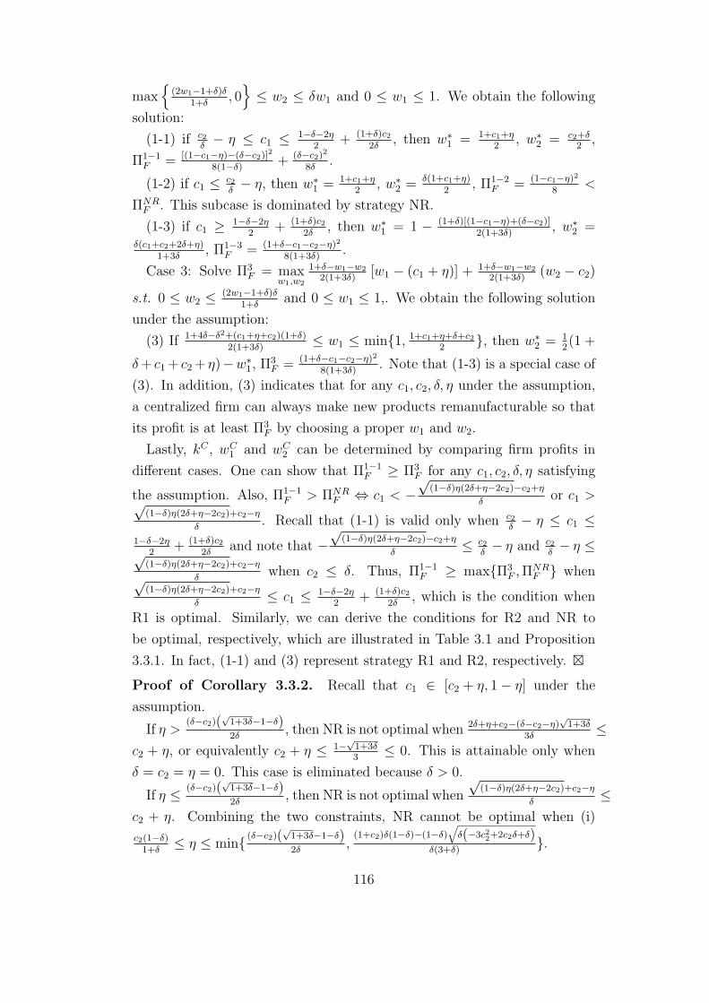
max

(2w1−1+δ)δ1+δ

, 0

≤ w2 ≤ δw1 and 0 ≤ w1 ≤ 1. We obtain the following

solution:

(1-1) if c2δ− η ≤ c1 ≤ 1−δ−2η

2+ (1+δ)c2

2δ, then w∗

1 = 1+c1+η2

, w∗2 = c2+δ

2,

Π1−1F = [(1−c1−η)−(δ−c2)]

2

8(1−δ)+ (δ−c2)

2

8δ.

(1-2) if c1 ≤ c2δ− η, then w∗

1 = 1+c1+η2

, w∗2 = δ(1+c1+η)

2, Π1−2

F = (1−c1−η)2

8<

ΠNRF . This subcase is dominated by strategy NR.

(1-3) if c1 ≥ 1−δ−2η2

+ (1+δ)c22δ

, then w∗1 = 1 − (1+δ)[(1−c1−η)+(δ−c2)]

2(1+3δ), w∗

2 =δ(c1+c2+2δ+η)

1+3δ, Π1−3

F = (1+δ−c1−c2−η)2

8(1+3δ).

Case 3: Solve Π3F = max

w1,w2

1+δ−w1−w2

2(1+3δ)[w1 − (c1 + η)] + 1+δ−w1−w2

2(1+3δ)(w2 − c2)

s.t. 0 ≤ w2 ≤ (2w1−1+δ)δ1+δ

and 0 ≤ w1 ≤ 1,. We obtain the following solution

under the assumption:

(3) If 1+4δ−δ2+(c1+η+c2)(1+δ)2(1+3δ)

≤ w1 ≤ min1, 1+c1+η+δ+c22

, then w∗2 = 1

2(1 +

δ+ c1+ c2+ η)−w∗1, Π

3F = (1+δ−c1−c2−η)2

8(1+3δ). Note that (1-3) is a special case of

(3). In addition, (3) indicates that for any c1, c2, δ, η under the assumption,

a centralized firm can always make new products remanufacturable so that

its profit is at least Π3F by choosing a proper w1 and w2.

Lastly, kC , wC1 and wC

2 can be determined by comparing firm profits in

different cases. One can show that Π1−1F ≥ Π3

F for any c1, c2, δ, η satisfying

the assumption. Also, Π1−1F > ΠNR

F ⇔ c1 < −√

(1−δ)η(2δ+η−2c2)−c2+η

δor c1 >√

(1−δ)η(2δ+η−2c2)+c2−η

δ. Recall that (1-1) is valid only when c2

δ− η ≤ c1 ≤

1−δ−2η2

+ (1+δ)c22δ

and note that −√

(1−δ)η(2δ+η−2c2)−c2+η

δ≤ c2

δ− η and c2

δ− η ≤√

(1−δ)η(2δ+η−2c2)+c2−η

δwhen c2 ≤ δ. Thus, Π1−1

F ≥ maxΠ3F ,Π

NRF when√

(1−δ)η(2δ+η−2c2)+c2−η

δ≤ c1 ≤ 1−δ−2η

2+ (1+δ)c2

2δ, which is the condition when

R1 is optimal. Similarly, we can derive the conditions for R2 and NR to

be optimal, respectively, which are illustrated in Table 3.1 and Proposition

3.3.1. In fact, (1-1) and (3) represent strategy R1 and R2, respectively. Proof of Corollary 3.3.2. Recall that c1 ∈ [c2 + η, 1− η] under the

assumption.

If η >(δ−c2)(

√1+3δ−1−δ)2δ

, then NR is not optimal when 2δ+η+c2−(δ−c2−η)√1+3δ

3δ≤

c2 + η, or equivalently c2 + η ≤ 1−√1+3δ3

≤ 0. This is attainable only when

δ = c2 = η = 0. This case is eliminated because δ > 0.

If η ≤ (δ−c2)(√1+3δ−1−δ)2δ

, then NR is not optimal when

√(1−δ)η(2δ+η−2c2)+c2−η

δ≤

c2 + η. Combining the two constraints, NR cannot be optimal when (i)

c2(1−δ)1+δ

≤ η ≤ min (δ−c2)(√1+3δ−1−δ)2δ

,(1+c2)δ(1−δ)−(1−δ)

√δ(−3c22+2c2δ+δ)

δ(3+δ).

116

Table B.2: D2’s Optimal Strategy in the Decentralized Scenario when k = 1

Case Condition d∗1 d∗2 w∗2

A c2δ ≤ w1 ≤ 2(1−δ)

3−δ + (1+δ)c2(3−δ)δ

12 − (2−δ)w1−c2

4(1−δ)w1δ−c24(1−δ)δ

w1δ+c22

B 1+4δ−δ2+(1+δ)c21+5δ ≤ w1 ≤ 1 1+δ−w1−c2

4(1+3δ) d∗11+δ−w1

2

C 2(1−δ)δ+(1+δ)c2(3−δ)δ ≤ w1 ≤ 1

2 − (1+δ)(δ−c2)1+5δ

1−w12(1+δ) d∗1

(2w1−1+δ)δ1+δ

(1+c2)δ(1−δ)−(1−δ)√

δ(δ+2c2δ−3c22)

δ(3+δ)≥ c2(1−δ)

1+δrequires that δ = c2 = 1 or c2 = 0;

or (ii) max c2(1−δ)1+δ

,(1+c2)δ(1−δ)+(1−δ)

√δ(δ+2c2δ−3c22)

δ(3+δ) ≤ η ≤ (δ−c2)(

√1+3δ−1−δ)2δ

.

(1+c2)δ(1−δ)+(1−δ)√

δ(δ+2c2δ−3c22)

δ(3+δ)≤ (δ−c2)(

√1+3δ−1−δ)2δ

requires that δ = c2 = 0 or

δ = c2 = 1 since δ ≥ c2.

In both case (i) and (ii), η = 0. Also, δ > 0 and c2 < 1⇒c2 = η = 0. Proof of Proposition 3.3.3 and the Optimal Solution. To prove part

(i)-(ii), we first solve the sequential game with backward induction.

Firstly, we solve the retailer’s problem. The retailer’s problem is the

same in the centralized and decentralized scenarios. Thus, the solution is

illustrated in Table B.1.

Secondly, we solve D2’s problem. If k = 0, then D2 makes no production

and ΠNR2 = 0. Given w1, if k = 1, we need to solve D2’s problem Π∗

2 =

maxw2

d2 (w2 − c2) and then D1’s problem. Note that D2 will remanufacture

only if Π∗2 ≥ 0, which implies that w2 ≥ c2 must hold. Similar to the

centralized scenario, it is not optimal for D1 to choose k = 1 if w2 ≥ δw1.

Thus, we only need to consider two cases given in Table B.1: Case 1 (Π2 =

maxw2≥c2

δw1−w2

2(1−δ)δ(w2 − c2) s.t. max

(2w1−1+δ)δ

1+δ, 0

≤ w2 ≤ δw1) and Case 3

(Π2 = maxw2≥c2

1+δ−w1−w2

2(1+3δ)(w2 − c2) s.t. 0 ≤ w2 ≤ (2w1−1+δ)δ

1+δ). In a similar

fashion to the proof of Proposition 3.3.1, we obtain D2’s strategy, which is

summarized in Table B.2:

Thirdly, we solve D1’s problem. If k = 0, then D1 sets wNR1 = 1+c1

2.

Consequently, dNR1 = 1−c1

4, ΠNR

1 = (1−c1)2

8. Note that D1 can always choose

k = 0 and earn at least ΠNR1 . If k = 1, then ΠR

1 = maxw1≥C1

d1 (w1 − C1), where

d1 is given in Table B.2 and C1 = c1 + η. Note that D1 will not choose a

remanufacturable product design if Π1 < 0, which implies that w1 ≥ C1 must

hold. Thus, we consider the following three cases:

Case A ( c2δ≤ w1 ≤ 2(1−δ)

3−δ+ (1+δ)c2

(3−δ)δ): Π1 = max

w1≥C1

2(1−δ)−(2−δ)w1+c24(1−δ)

(w1 − C1)

117

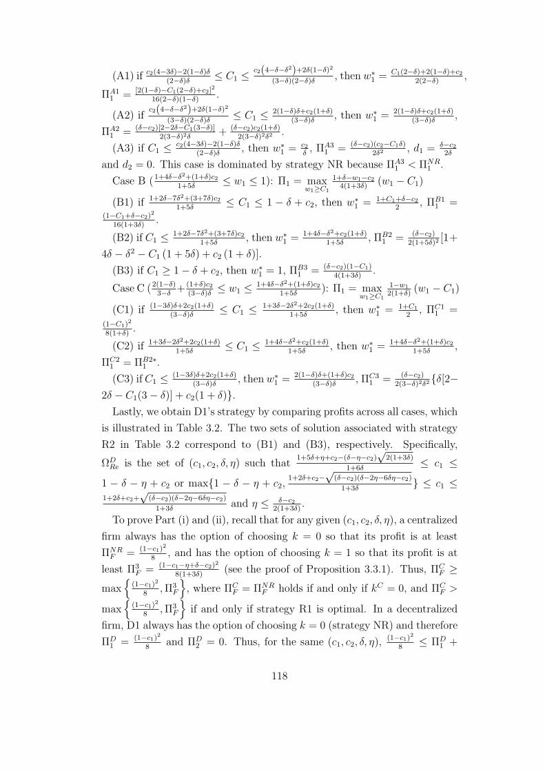
(A1) if c2(4−3δ)−2(1−δ)δ(2−δ)δ

≤ C1 ≤c2(4−δ−δ2)+2δ(1−δ)2

(3−δ)(2−δ)δ, then w∗

1 =C1(2−δ)+2(1−δ)+c2

2(2−δ),

ΠA11 = [2(1−δ)−C1(2−δ)+c2]

2

16(2−δ)(1−δ).

(A2) ifc2(4−δ−δ2)+2δ(1−δ)2

(3−δ)(2−δ)δ≤ C1 ≤ 2(1−δ)δ+c2(1+δ)

(3−δ)δ, then w∗

1 = 2(1−δ)δ+c2(1+δ)(3−δ)δ

,

ΠA21 = (δ−c2)[2−2δ−C1(3−δ)]

2(3−δ)2δ+ (δ−c2)c2(1+δ)

2(3−δ)2δ2.

(A3) if C1 ≤ c2(4−3δ)−2(1−δ)δ(2−δ)δ

, then w∗1 = c2

δ, ΠA3

1 = (δ−c2)(c2−C1δ)2δ2

, d1 =δ−c22δ

and d2 = 0. This case is dominated by strategy NR because ΠA31 < ΠNR

1 .

Case B (1+4δ−δ2+(1+δ)c21+5δ

≤ w1 ≤ 1): Π1 = maxw1≥C1

1+δ−w1−c24(1+3δ)

(w1 − C1)

(B1) if 1+2δ−7δ2+(3+7δ)c21+5δ

≤ C1 ≤ 1 − δ + c2, then w∗1 = 1+C1+δ−c2

2, ΠB1

1 =(1−C1+δ−c2)

2

16(1+3δ).

(B2) if C1 ≤ 1+2δ−7δ2+(3+7δ)c21+5δ

, then w∗1 =

1+4δ−δ2+c2(1+δ)1+5δ

, ΠB21 = (δ−c2)

2(1+5δ)2[1+

4δ − δ2 − C1 (1 + 5δ) + c2 (1 + δ)].

(B3) if C1 ≥ 1− δ + c2, then w∗1 = 1, ΠB3

1 = (δ−c2)(1−C1)4(1+3δ)

.

Case C (2(1−δ)3−δ

+ (1+δ)c2(3−δ)δ

≤ w1 ≤ 1+4δ−δ2+(1+δ)c21+5δ

): Π1 = maxw1≥C1

1−w1

2(1+δ)(w1 − C1)

(C1) if (1−3δ)δ+2c2(1+δ)(3−δ)δ

≤ C1 ≤ 1+3δ−2δ2+2c2(1+δ)1+5δ

, then w∗1 = 1+C1

2, ΠC1

1 =(1−C1)

2

8(1+δ).

(C2) if 1+3δ−2δ2+2c2(1+δ)1+5δ

≤ C1 ≤ 1+4δ−δ2+c2(1+δ)1+5δ

, then w∗1 = 1+4δ−δ2+(1+δ)c2

1+5δ,

ΠC21 = ΠB2∗

1 .

(C3) if C1 ≤ (1−3δ)δ+2c2(1+δ)(3−δ)δ

, then w∗1 =

2(1−δ)δ+(1+δ)c2(3−δ)δ

, ΠC31 = (δ−c2)

2(3−δ)2δ2δ[2−

2δ − C1(3− δ)] + c2(1 + δ).Lastly, we obtain D1’s strategy by comparing profits across all cases, which

is illustrated in Table 3.2. The two sets of solution associated with strategy

R2 in Table 3.2 correspond to (B1) and (B3), respectively. Specifically,

ΩDRe is the set of (c1, c2, δ, η) such that

1+5δ+η+c2−(δ−η−c2)√

2(1+3δ)

1+6δ≤ c1 ≤

1 − δ − η + c2 or max1 − δ − η + c2,1+2δ+c2−

√(δ−c2)(δ−2η−6δη−c2)

1+3δ ≤ c1 ≤

1+2δ+c2+√

(δ−c2)(δ−2η−6δη−c2)

1+3δand η ≤ δ−c2

2(1+3δ).

To prove Part (i) and (ii), recall that for any given (c1, c2, δ, η), a centralized

firm always has the option of choosing k = 0 so that its profit is at least

ΠNRF = (1−c1)

2

8, and has the option of choosing k = 1 so that its profit is at

least Π3F = (1−c1−η+δ−c2)2

8(1+3δ)(see the proof of Proposition 3.3.1). Thus, ΠC

F ≥

max

(1−c1)2

8,Π3

F

, where ΠC

F = ΠNRF holds if and only if kC = 0, and ΠC

F >

max

(1−c1)2

8,Π3

F

if and only if strategy R1 is optimal. In a decentralized

firm, D1 always has the option of choosing k = 0 (strategy NR) and therefore

ΠD1 = (1−c1)

2

8and ΠD

2 = 0. Thus, for the same (c1, c2, δ, η),(1−c1)

2

8≤ ΠD

1 +

118

ΠD2 ≤ max

(1−c1)

2

8, 3(1−c1−η+δ−c2)

2

32(1+3δ), (δ−c2)[2(1−c1−η)+δ−c2]

8(1+3δ)

(see the above proof

of Proposition 3.3.3), where ΠD1 + ΠD

2 = (1−c1)2

8⇔ kD = 0. One can show

that max

3(1−c1−η+δ−c2)2

32(1+3δ), (δ−c2)[2(1−c1−η)+δ−c2]

8(1+3δ)

< (1−c1−η+δ−c2)2

8(1+3δ)because 1−

c1 − η > 0 and δ − c2 ≥ 0. Thus, ΠD1 + ΠD

2 ≤ ΠCF for ∀ (c1, c2, δ, η) ∈ Ω.

Specifically, ΠD1 +ΠD

2 = ΠCF ⇔ ΠD

1 +ΠD2 = (1−c1)

2

8= ΠC

F ⇔ kC = kD = 0.

Next, we prove ΩDRe ⊂ ΩC

Re by showing that (c1, c2, δ, η) ∈ ΩDRe ⇒ (c1, c2, δ, η) ∈

ΩCRe. For ∀ (c1, c2, δ, η) ∈ ΩD

Re, either ΠD1 + ΠD

2 = 3(1−c1−η+δ−c2)2

32(1+3δ)> (1−c1)

2

8or

ΠD1 + ΠD

2 = (δ−c2)[2(1−c1−η)+δ−c2]8(1+3δ)

> (1−c1)2

8must hold. For the same choice of

(c1, c2, δ, η), the centralized firm’s profit satisfies ΠCF ≥ (1−c1−η+δ−c2)2

8(1+3δ)if k = 1

and ΠCF = (1−c1)

2

8if k = 0. One can show that given the above (c1, c2, δ, η) ∈

ΩCRe,

(1−c1−η+δ−c2)2

8(1+3δ)> max

3(1−c1−η+δ−c2)

2

32(1+3δ), (δ−c2)[2(1−c1−η)+δ−c2]

8(1+3δ)

> (1−c1)

2

8.

Therefore, kC = 1, or equivalently, (c1, c2, δ, η) ∈ ΩCRe.

Part (iii). ΩDRe ⊂ ΩC

Re ⇒ if (c1, c2, δ, η) is such that kD = 1, then kC = 1 for

the same (c1, c2, δ, η). Also, according to Table 3.2, dD1 = dD2 when kD = 1.

Therefore, to show dD1 = dD2 < dC1 , we only need to compare(dD1−1, d

D1−2

)=(

1−c1−η+δ−c28(1+3δ)

, δ−c24(1+3δ)

)with

(dC1−1, d

C1−2

)=

(1−c1−η−δ+c2

4(1−δ), 1−c1−η+δ−c2

4(1+3δ)

). One

can show that maxdD1−1, d

D1−2

< dC1−2 because 1− c1 − η > 0 and δ − c2 ≥

0. Also, maxdD1−1, d

D1−2

< dC1−1 when c1 < 1−δ−2η

2+ (1+δ)c2

2δ(a necessary

condition for dC1 = dC1−1). Hence, dD1 < dC1 .

Similarly, to show dD1 +dD2 < dC1 +dC2 , we only need to compare dD1−1+dD2−1 =1−c1−η+δ−c2

8(1+3δ)+ 1−c1−η+δ−c2

8(1+3δ)= 1−c1−η+δ−c2

4(1+3δ)and dD1−2+ dD2−2 =

δ−c24(1+3δ)

+ δ−c24(1+3δ)

=δ−c2

2(1+3δ)with dC1−1 + dC2−1 =

1−c1−η−δ+c24(1−δ)

+ δ(c1+η)−c24(1−δ)δ

= δ−c24δ

and dC1−2 + dC2−2 =1−c1−η+δ−c2

4(1+3δ)+ 1−c1−η+δ−c2

4(1+3δ)= 1−c1−η+δ−c2

2(1+3δ). One can show that maxdD1−1 +

dD2−1, dD1−2 + dD2−2 < dC1−2 + dC2−2 because 1− c1 − η > 0 and δ− c2 ≥ 0. Also,

maxdD1−1+dD2−1, dD1−2+dD2−2 < dC1−1+dC2−1 when

1+2δ−7δ2+(3+7δ)c21+5δ

−η ≤ c1 (a

necessary condition for dD1 = dD1−1 and dD2 = dD2−1). Hence, dD1 +dD2 < dC1 +dC2 .

The remaining results are directly obtained from Table 3.2. Proof of Proposition 3.4.2: Firstly, we solve the retailer’s problem. Table

B.1 illustrated the optimal solution.

Secondly, we solve D2’s problem. If k = 0, then D2 makes no production

and ΠNR2 = 0. If k = 1 and D2 chooses j = 0, then the problem is essentially

the same as in the decentralized scenario. Thus, in the following analysis,

we only need to solve D2’s problem Π∗2 = max

w2

d2 (w2 − c2) − d1τ − f when

k = 1 and j = 1, where d1 and d2 are given in Table B.1. Note that f is

119

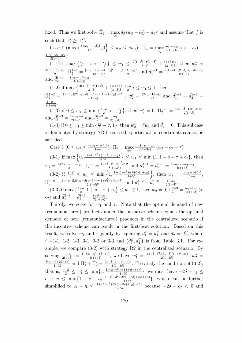
fixed. Thus we first solve Π2 = maxw2

d2 (w2 − c2)− d1τ and assume that f is

such that Π∗2 ≥ ΠD

2 .

Case 1 (max

(2w1−1+δ)δ1+δ

, 0

≤ w2 ≤ δw1): Π2 = maxw2

δw1−w2

2(1−δ)δ(w2 − c2) −

1−δ−w1+w2

2(1−δ)τ

(1-1) if max

c2δ− τ, τ − c2

δ

≤ w1 ≤ 2(1−δ)−τ(1+δ)

3−δ+ (1+δ)c2

(3−δ)δ, then w∗

2 =δ(w1−τ)+c2

2, Π1−1

2 = [δw1+τ(2−δ)−c2]2

8(1−δ)δ− (τ+δ−c2)τ

2δand d1−1

1 = 2(1−δ)−(2−δ)w1−δτ+c24(1−δ)

and d1−12 = (w1+τ)δ−c2

4(1−δ)δ.

(1-2) if max

2(1−δ)−τ(1+δ)3−δ

+ c2(1+δ)(3−δ)δ

, 1−δ2

≤ w1 ≤ 1, then

Π1−22 = (1−w1)[2δw1−δ(1−δ)−τ(1+δ)−c2(1+δ)]

2(1+δ)2, w∗

2 = (2w1−1+δ)δ1+δ

and d1−21 = d1−2

2 =1−w1

2(1+δ).

(1-3) if 0 ≤ w1 ≤ min

1−δ2, τ − c2

δ

, then w∗

2 = 0, Π1−32 = (w1+δ−1)τ−c2w1

2(1−δ)

and d1−31 = 1−w1−δ

2(1−δ)and d1−3

2 = w1

2(1−δ).

(1-4) if 0 ≤ w1 ≤ min

c2δ− τ, 1

, then w∗

2 = δw1 and d2 = 0. This subcase

is dominated by strategy NR because the participation constraints cannot be

satisfied.

Case 3 (0 ≤ w2 ≤ (2w1−1+δ)δ1+δ

): Π2 = maxw2

1+δ−w1−w2

2(1+3δ)(w2 − c2 − τ)

(3-1) if max0, 1+4δ−δ2+(1+δ)(τ+c2)

1+5δ

≤ w1 ≤ min 1, 1 + δ + τ + c2, then

w2 =1+δ+τ−w1+c2

2, Π3−1

2 = (1+δ−τ−w1−c2)2

8(1+3δ)and d3−1

1 = d3−12 = 1+δ−τ−w1−c2

4(1+3δ).

(3-2) if 1−δ2

≤ w1 ≤ min1, 1+4δ−δ2+(1+δ)(τ+c2)

1+5δ

, then w2 = (2w1−1+δ)δ

1+δ,

Π3−22 = (1−w1)[2δw1−δ(1−δ)−τ(1+δ)−c2(1+δ)]

2(1+δ)2and d3−2

1 = d3−22 = 1−w1

2(1+δ).

(3-3) if max

1−δ2, 1 + δ + τ + c2

≤ w1 ≤ 1, then w2 = 0, Π3−3

2 = w1−δ−12(1+3δ)

(τ+

c2) and d3−31 = d3−3

2 = 1+δ−w1

2(1+3δ).

Thirdly, we solve for w1 and τ . Note that the optimal demand of new

(remanufactured) products under the incentive scheme equals the optimal

demand of new (remanufactured) products in the centralized scenario if

the incentive scheme can result in the first-best solution. Based on this

result, we solve w1 and τ jointly by equating di1 = dC1 and di2 = dC2 , where

i =1-1, 1-2, 1-3, 3-1, 3-2 or 3-3 and(dC1 , d

C2

)is from Table 3.1. For ex-

ample, we compare (3-2) with strategy R2 in the centralized scenario: By

solving 1−w1

2(1+δ)= 1−(c1+η)+(δ−c2)

4(1+3δ), we have w∗

1 = 1+4δ−δ2+(1+δ)(c1+η+c2)2(1+3δ)

, w∗2 =

δ(c1+η+2δ+c2)1+3δ

and Π∗1 +Π∗

2 =(1+δ−c1−c2−η)2

8(1+3δ). To satisfy the condition of (3-2),

that is, 1−δ2

≤ w∗1 ≤ min1, 1+4δ−δ2+(1+δ)(τ+c2)

1+5δ, we must have −2δ − c2 ≤

c1 + η ≤ min1 + δ − c2,1+4δ−δ2+2τ(1+3δ)+c2(1+δ)

1+5δ, which can be further

simplified to c1 + η ≤ 1+4δ−δ2+2τ(1+3δ)+c2(1+δ)1+5δ

because −2δ − c2 < 0 and

120

1 + δ − c2 > 1. In a similar fashion, we obtain the following cases:

(A1) If k = 1 and c2δ

≤ c1 + η ≤ 1−δ2

+ (1+δ)c22δ

, then wA11 = 1+(c1+η)

2,

wA12 = δ+c2

2, τA1 = c1+η−1

2, ΠA1

1 = f , ΠA12 = (1−c1−η−δ+c2)2

8(1−δ)+ (δ−c2)

2

8δ−f , ΠA1

1 +

ΠA12 = (1−c1−η−δ+c2)2

8(1−δ)+ (δ−c2)

2

8δ, dA1

1 = 1−(c1+η)−(δ−c2)4(1−δ)

, and dA12 = δ(c1+η)−c2

4(1−δ)δ.

(A2) If k = 1 and 1−4δ−δ2−2τ(1+3δ)3−δ

+ c2(2+δ)(1+δ)(3−δ)δ

≤ c1 + η, then wA21 =

1+4δ−δ2+(1+δ)(c1+η+c2)2(1+3δ)

, wA22 = 1+4δ−δ2+(1+δ)(c1+η+c2)

2(1+3δ),

ΠA21 =

(1−c1−η+δ−c2)[1+4δ−δ2−(1+5δ)(c1+η)+2τ(1+3δ)+c2(1+δ)]8(1+3δ)2

+ f ,

ΠA22 = (1−c1−η+δ−c2)[δ(c1+η+2δ)−c2(1+2δ)−τ(1+3δ)]

4(1+3δ)2−f , ΠA2

1 +ΠA22 = (1+δ−c1−c2−η)2

8(1+3δ),

and dA21 = dA2

2 = 1−(c1+η)+(δ−c2)4(1+3δ)

.

(A3) If k = 1 and c1 + η ≤ 1+4δ−δ2+2τ(1+3δ)+c2(1+δ)1+5δ

, then wA31 = wA2

1 ,

wA32 = wA2

2 , ΠA31 = ΠA2

1 , ΠA32 = ΠA2

2 , ΠA31 + ΠA3

2 = (1+δ−c1−c2−η)2

8(1+3δ), and

dA31 = dA3

2 = 1−(c1+η)+(δ−c2)4(1+3δ)

.

(A4) If k = 1 and maxτ, 1+4δ−δ2+2τ(1+3δ)+c2(1+δ)1+5δ

≤ c1 + η ≤ min1 +

τ, 1 + δ + 2τ + c2, then wA41 = c1 + η − τ , wA4

2 = 1−c1−η+δ+c22

+ τ , ΠA41 = f ,

ΠA42 = (1+δ−c1−c2−η)2

8(1+3δ)− f , ΠA4

1 + ΠA42 = (1+δ−c1−c2−η)2

8(1+3δ), and dA4

1 = dA42 =

1−(c1+η)+(δ−c2)4(1+3δ)

.

(A5) If k = 1 and 1 + δ + 2τ + c2 ≤ c1 + η ≤ 1 − δ − c2, then wA51 =

1+(c1+η)+δ+c22

, wA42 = 0, ΠA5

1 = (1−c1−η+δ−c2)(1−c1−η+δ+2τ+c2)8(1+3δ)

+ f , ΠA52 =

−(1−c1−η+δ−c2)(τ+c2)4(1+3δ)

− f , ΠA51 + ΠA5

2 = (1+δ−c1−c2−η)2

8(1+3δ), and dA5

1 = dA52 =

1−(c1+η)+(δ−c2)4(1+3δ)

.

(A6) If k = 0, then wA61 = 1+c1

2, ΠA6

1 = (1−c1)2

8, and dA6

1 = 1−c14

.

Note that the above cases are not exclusive. However, similar to the profit

comparison procedure mentioned in the proof of Proposition 3.3.1, we can

derive the optimal strategy and the corresponding conditions (illustrated in

Table 3.1) except the value of w∗1 and w∗

2 when strategy R2 is optimal. Thus,

we have proven part (iii) of Proposition 3.4.2.

Proposition 3.4.2(i): if (c1, c2, δ, η) ∈ ΩCR1, then the optimal τ is directly

derived from (A1) in the proof of Proposition 3.4.2. Recall that the participa-

tion constraint for D1 is ΠT1 > ΠD

1 , where ΠD1 ≥ (1−c1)2

8. Thus, fT > (1−c1)2

8>

0. Given that c1 ≥√

(1−δ)η(2δ+η−2c2)+c2−η

δand

√(1−δ)η(2δ+η−2c2)+c2−η

δ≥ c2

δ− η

when δ ≥ c2, we have c1 ≥ c2δ− η, or equivalently, c2 ≤ δ(η + c1). One can

show that dT1 · τT + fT ≥ η[2(1−c1−η)+η]8

≥ 0. Thus, fT > 0 because τT < 0

and dT1 > 0.

Proposition 3.4.2(ii): if (c1, c2, δ, η) ∈ ΩCR2 and τ = 0, then (A2)-(A4)

121

Table B.3: The Retailer’s Optimal Strategy (w1, w2 ≥ 0)

Case Cond. d∗1 d∗2

1 k = 1 & max

(2w1−1+δ)δ1+δ , 0

≤ w2 ≤ δw1

1−δ−w1+w22(1−δ)

δw1−w22(1−δ)δ

2 k = 1 & w2 ≥ δw1 & w1 ≤ 1 or k = 0 & w1 ≤ 1 1−w12 0

3 k = 1 & 0 ≤ w2 ≤ min

(2w1−1+δ)δ1+δ , 1 + δ − w1

1+δ−w1−w2

2(1+3δ)1+δ−w1−w2

2(1+3δ)

Case Π∗R

1w2

2−2w1w2δ+(1+w21−2w1(1−δ)−δ)δ

4(1−δ)δ

2 (1−w1)2

4

3 (1−w1−w2+δ)2

4(1+3δ)

constitute the optimal solutions when R2 is optimal. That is, one of the

three cases is associated with the optimal solution and the corresponding

(τ, f) enables the firm to achieve the first-best profit. Letting τ = 0 and

given that 1 + δ + c2 ≥ 1 and c1 + η ∈ [0, 1], the condition for (A2)-(A4)

can be simplified to 1−4δ−δ2

3−δ+ c2(2+δ)(1+δ)

(3−δ)δ≤ c1 + η, c1 + η ≤ 1+4δ−δ2+c2(1+δ)

1+5δ

and 1+4δ−δ2+c2(1+δ)1+5δ

≤ c1 + η, respectively. Next, we show that fT > 0 for

all three cases. Note that the participation constraint for D1 is ΠT1 > ΠD

1 ,

where ΠD1 ≥ (1−c1)2

8. If (A4) is associated with the optimal solution, then

ΠT1 = fT > (1−c1)2

8> 0 holds when τ = 0. Similarly, if (A2) or (A3)

is associated with the optimal solution, then ΠT1 > (1−c1)2

8should also hold.

One can show that fT > ΠT1 −

(1−c1)2

8= 1

8(1+3δ)2(1+5δ)(1−c1)

2−(1+5δ)(1−c1−η)2+(1−c1)

2δ(1+5δ)+[2(1−c1)δ−δ+c2]2+4δη(δ−c2)+δ(δ−c2)

2 > 0

when τ = 0. Proof of Proposition 3.4.1: This can be directly derived from Proposition

3.4.2(i): In order to achieve the first-best firm profit ΠCF , τ

V = c1+η−12

must

hold. Otherwise, one of the following three cases would happen: 1) kV = 0

and hence ΠV1 = (1−c1)

2

8,ΠV

2 = 0; 2) kV = 1 but D2 opts out (j = 0) and

hence ΠVi = ΠD

i (i = 1, 2); 3) kV = 1 and j = 1 but ΠV1 + ΠV

2 < ΠCF

according to Proposition 3.4.2(i). In each case, ΠV1 + ΠV

2 < ΠCF will always

hold. However, if τV = c1+η−12

, then ΠV1 = 0, which violates the participation

constraint according to Proposition 3.4.2(i). Model Extension 1: No upper limit on wholesale prices

1.1. The Centralized Scenario: Similar to the proof of Proposition 3.3.1,

we obtain the retailer’s optimal strategy (see Table B.3) and the firm’s opti-

122

Table B.4: D2’s Optimal Strategy in the Decentralized Scenario(w1, w2 ≥ 0)

Case Cond. d∗1 d∗2 w∗2

1 c2δ ≤ w1 ≤ 2(1−δ)

3−δ + (1+δ)c2(3−δ)δ

12 − (2−δ)w1−c2

4(1−δ)w1δ−c24(1−δ)δ

w1δ+c22

2 2(1−δ)δ+(1+δ)c2(3−δ)δ ≤ w1 ≤ 1− (1+δ)(δ−c2)

1+5δ1−w12(1+δ) d∗1

(2w1−1+δ)δ1+δ

3 1+4δ−δ2+(1+δ)c21+5δ ≤ w1 ≤ 1 + δ − c2

1+δ−w1−c24(1+3δ) d∗1

1+δ−w12

Table B.5: Optimal Strategy and Solutions in the Decentralized Scenario(w1, w2 ≥ 0)

Strategy Cond. wD1 wD

2 dD1 dD2

R2 (*) 1+c1+η+δ−c22

1−c1−η+δ+c24

1−c1−η+δ−c28(1+3δ) dD1

NR otherwise 1+c12 − 1−c1

4 −

Strategy ΠD1 ΠD

2 ΠDR

R2 (1−c1−η+δ−c2)2

16(1+3δ)ΠD

1

2ΠD

1

4

NR (1−c1)2

8 − ΠD1

2

(*) c1 ≥ 1+5δ+η+c2−(δ−η−c2)√

2(1+3δ)

1+6δ

mal strategy. One can show that Proposition 3.3.1 and the optimal solution

(see Table 3.1) still hold, except that when R2 is optimal, w1 must satisfy1+4δ−δ2+(c1+η+c2)(1+δ)

2(1+3δ)≤ w1 ≤ 1+δ+c1+η+c2

2, which is a relaxed condition, as

compared to the constraint on w1 in the benchmark model.

1.2. The Decentralized Scenario: Again, we obtain the equilibrium so-

lutions by solving the problem backward. Similar to the proof of Proposition

3.3.3, one can derive the optimal strategy of the retailer (see Table B.3), of

D2 (see Table B.4) and of D1 (see Table B.5).

Based on Table B.5, one can show the part (i)-(iii) of Proposition 3.3.3

still hold when there are no upper limits on w1 and w2.

1.3. The Two-part Coordination Scheme: Similar to the proof of

Proposition 3.4.2, one can show that the optimal strategies and the corre-

sponding conditions are the same with and without the upper limits on w1

and w2 except the value of w∗1 and w∗

2 when strategy R2 is optimal.

Model Extension 2: No Retailer

2.1. The Centralized Scenario without the Retailer: If k = 0, then

p1 = 1 − d1. The firm’s problem is ΠNRF = max

d1d1 · (1− d1 − c1) s.t. 0 ≤

123

Table B.6: Optimal Solutions in the Centralized Scenario (No Retailer,w1, w2 ∈ [0, 1])

Strategy Cond. kC pC1 pC2R1 (*) 1 1+c1+η

2c2+δ2

R2 (**) 1 1+4δ−δ2+(c1+η+c2)(1+δ)2(1+3δ)

δ(c1+c2+2δ+η)1+3δ

NR o.w. 0 1+c12 −

Strategy dC1 dC2 ΠCF

R11−c1−η−δ+c2

2(1−δ)δ(c1+η)−c22(1−δ)δ

(1−c1−η−δ+c2)2

4(1−δ) + (δ−c2)2

4δ

R21+δ−c1−η−c2

2(1+3δ) dC1(1−c1−η+δ−c2)

2

4(1+3δ)

NR1−c12 − (1−c1)

2

4

(*) and (**) correspond to the condition when R1 and R2 are optimal based on

Proposition 3.3.1, respectively.

d1 ≤ 1. Thus, we have dNR1 = 1−c1

2, pNR

1 = 1+c12

and ΠNRF = (1−c1)

2

4. If

k = 1, then p1 = 1− d1 − δd2 and p2 = δ(1− d1 − d2). The firm’s problem is

ΠF = maxd1,d2 d1(1−d1−δd2−c1−η)+d2[δ(1−d1−d2)−c2] s.t. d1−d2 ≥ 0,

1 − d1 − d2 ≥ 0 and d1, d2 ≥ 0. Similar to the proof of Proposition 3.3.1,

we derive the condition when each strategy is optimal and summarize the

results in Table B.6.

2.2. The Decentralized Scenario without the Retailer: In this sce-

nario, D1 decides kD and p1 ∈ [0, 1], and D2 decides p2 ∈ [0, 1]. Note

that here we cannot formulate retail prices using (3.1)-(3.2) of the paper

because neither division can exclusively determines the sales of new or re-

manufactured products when kD = 1. By simultaneously solving p1 =

1 − d1 − δd2 and p2 = δ(1 − d1 − d2), we obtain d1 = 1−δ−p1+p21−δ

and

d2 = δp1−p2(1−δ)δ

. d1 ≥ d2 ⇒ p2 ≥ (2p1−1+δ)δ1+δ

. Also note that if p2 < (2p1−1+δ)δ1+δ

,

then D2 can always increase p2 to (2p1−1+δ)δ1+δ

so that D2’s profit and sales

of remanufactured products both increase. Hence, it is not optimal for D2

to price remanufactured products at p2 < (2p1−1+δ)δ1+δ

. Meanwhile, d2 ≥ 0 ⇒p2 ≤ δp1. Thus, in the decentralized scenario without vertical integration,

D1’s profit is ΠNR1 = max

p1(1 − p1) · (p1 − c1) s.t. c1 ≤ p1 ≤ 1 when

k = 0 and ΠRE1 = max

p1

1−δ−p1+p21−δ

(p1 − c1 − η) s.t. c1 + η ≤ p1 ≤ 1 when

k = 1. Thus, D1 optimal profit is ΠD1 = maxΠNR

1 ,ΠRE1 ; the optimal

design decision kD = 0 ⇔ ΠNR1 ≥ ΠRE

1 . Given k = 1 and p1, D2’s problem is

ΠD2 = max

p2

δp1−p2(1−δ)δ

(p2 − c2) s.t. maxc2, (2p1−1+δ)δ1+δ

≤ p2 ≤ δp1. D2’s optimal

strategy is illustrated in Table B.7:

124

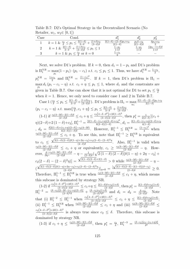
Table B.7: D2’s Optimal Strategy in the Decentralized Scenario (NoRetailer, w1, w2∈ [0, 1])

Case Cond. d∗1 d∗2 p∗21 k = 1 & c2

δ ≤ p1 ≤ 2(1−δ)3−δ + (1+δ)c2

(3−δ)δ2(1−δ)−(2−δ)p1+c2

2(1−δ)p1δ−c22(1−δ)δ

δp1+c22

2 k = 1 & 2(1−δ)3−δ + (1+δ)c2

(3−δ)δ ≤ p1 ≤ 1 1−p11+δ

1−p11+δ

(2p1−1+δ)δ1+δ

3 k = 1 & p1 ≤ c2δ or k = 0 1−c1

2 − −

Next, we solve D1’s problem. If k = 0, then d1 = 1− p1 and D1’s problem

is ΠNR1 = max

p1(1−p1) · (p1 − c1) s.t. c1 ≤ p1 ≤ 1. Thus, we have dNR

1 = 1−c12

,

pNR1 = 1+c1

2and ΠNR

1 = (1−c1)2

4. If k = 1, then D1’s problem is Π1 =

maxp1

d1 (p1 − c1 − η) s.t. c1 + η ≤ p1 ≤ 1, where d1 and the constraints are

given in Table B.7. One can show that it is not optimal for D1 to set p1 ≤ c2δ

when k = 1. Hence, we only need to consider case 1 and 2 in Table B.7.

Case 1 ( c2δ≤ p1 ≤ 2(1−δ)

3−δ+ (1+δ)c2

(3−δ)δ). D1’s problem is Π1 = max

w1

2(1−δ)−(2−δ)p1+c22(1−δ)

(p1 − c1 − η) s.t. max c2δ, c1 + η ≤ p1 ≤ 2(1−δ)

3−δ+ (1+δ)c2

(3−δ)δ.

(1-1) if c2(4−3δ)−2(1−δ)δ(2−δ)δ

≤ c1+ η ≤ c2(4−δ−δ2)+2δ(1−δ)2

(3−δ)(2−δ)δ, then p∗1 =

12(2−δ)

[(c1+

η)(2−δ)+2 (1− δ)+c2], Π1−11 = [2(1−δ)−(c1+η)(2−δ)+c2]

2

8(2−δ)(1−δ), d1 =

2(1−δ)−(c1+η)(2−δ)+c24(1−δ)

, d2 = δ[2(1−δ)+(c1+η)(2−δ)]−c2(4−3δ)4(2−δ)(1−δ)δ

. However, Π1−11 ≤ ΠNR

1 = (1−c1)2

4when

c2(4−3δ)−2(1−δ)δ(2−δ)δ

≤ c1 + η. To see this, note that Π1−11 ≥ ΠNR

1 is equivalent

to c1 ≤√

2(1−δ)(2−δ)[δ(1−η)+2η−c2]+c2(2−δ)−(2−δ)2η

(2−δ)δ. Also, Π1−1

1 is valid whenc2(4−3δ)−2(1−δ)δ

(2−δ)δ≤ c1 + η or equivalently, c1 ≥ c2(4−3δ)−2(1−δ)δ

(2−δ)δ− η. How-

ever, ∂∂η[ c2(4−3δ)−2(1−δ)δ

(2−δ)δ− η − 1

(2−δ)δ(√

2 (1− δ) (2− δ)[δ(1 − η) + 2η − c2] +

c2(2 − δ) − (2 − δ)2η)] =

√2(1−δ)(2−δ)+2(1−δ)

δ> 0 while c2(4−3δ)−2(1−δ)δ

(2−δ)δ− η −

(

√2(1−δ)(2−δ)[δ(1−η)+2η−c2]+c2(2−δ)−(2−δ)2η

(2−δ)δ)|η=0 =

[√

2(1−δ)(2−δ)−2(1−δ)](δ−c2)

(2−δ)δ≥ 0.

Therefore, Π1−11 ≤ ΠNR

1 is true when c2(4−3δ)−2(1−δ)δ(2−δ)δ

≤ c1 + η, which means

this subcase is dominated by strategy NR.

(1-2) ifc2(4−δ−δ2)+2δ(1−δ)2

(3−δ)(2−δ)δ≤ c1+η ≤ 2(1−δ)δ+c2(1+δ)

(3−δ)δ, then p∗1 =

2(1−δ)δ+c2(1+δ)(3−δ)δ

,

Π1−21 = (δ−c2)[2−2δ−(c1+η)(3−δ)]

(3−δ)2δ+ (δ−c2)c2(1+δ)

(3−δ)2δ2and d1 = d2 = δ−c2

(3−δ)δ. Note

that (i) Π1−21 ≤ Π1−1

1 whenc2(4−δ−δ2)+2δ(1−δ)2

(3−δ)(2−δ)δ≤ c1 + η ≤ 2(1−δ)δ+c2(1+δ)

(3−δ)δ;

(ii) Π1−11 ≤ ΠNR

1 when c2(4−3δ)−2(1−δ)δ(2−δ)δ

≤ c1 + η and (iii) c2(4−3δ)−2(1−δ)δ(2−δ)δ

≤c2(4−δ−δ2)+2δ(1−δ)2

(3−δ)(2−δ)δis always true since c2 ≤ δ. Therefore, this subcase is

dominated by strategy NR.

(1-3) if c1 + η ≤ c2(4−3δ)−2(1−δ)δ(2−δ)δ

, then p∗1 = c2δ, Π1−3

1 = (δ−c2)[c2−(c1+η)δ]δ2

,

125

d1 =δ−c2δ

and d2 = 0. This case is dominated by strategy NR since d2 = 0.

Case 2 (2(1−δ)3−δ

+ (1+δ)c2(3−δ)δ

≤ p1 ≤ 1). D1’s problem is Π1 = maxp1

1−p11+δ

(p1 − C1)

s.t. maxC1,2(1−δ)3−δ

+ (1+δ)c2(3−δ)δ

≤ p1 ≤ 1, where C1 = c1 + η.

(2-1) p∗1 =1+C1

2; Π2−1

1 = (1−C1)2

4(1+δ); d1 = d2 =

1−C1

2(1+δ)when C1 ≥ (1−3δ)δ+2c2(1+δ)

(3−δ)δ.

However, this subcase is dominated by NR because Π2−11 = (1−C1)

2

4(1+δ)≤ (1−c1)

2

4=

ΠNR1 .

(2-2) p∗1 =2(1−δ)δ+(1+δ)c2

(3−δ)δ; µ∗

1 =2c2(1+δ)−3δ2+δ−C1δ(3−δ)

(3−δ)δ(δ+1); Π2−2

1 = (δ−c2)(3−δ)2δ2

δ[2−2δ − C1(3 − δ)] + c2(1 + δ); d1 = d2 = δ−c2

(3−δ)δwhen C1 ≤ (1−3δ)δ+2c2(1+δ)

(3−δ)δ.

However, this subcase is dominated by NR because (1−c1)2

4(1+δ)≥ (1−C1)

2

4(1+δ)≥

(δ−c2)δ[2(1−δ)−C1(3−δ)]+c2(1+δ)(3−δ)2δ2

.

In all, it is not optimal for D1 to choose a remanufacturable design.

2.3. Two-Part Coordination Scheme without the Retailer: Again,

we use backward induction, starting with D2’s profit maximization problem.

If k = 0, then D2’s profit is ΠNR2 = 0. If k = 1, then D2’s problem is

Π∗2 = max

p2

δp1−p2(1−δ)δ

(p2 − c2) − 1−δ−p1+p21−δ

· τ − f s.t. max0, (2p1−1+δ)δ1+δ

≤ p2 ≤

δp1. Given that f is fixed, we can first solve the following problem: Π2 =

maxp2

δp1−p2(1−δ)δ

(p2 − c2)− 1−δ−p1+p21−δ

· τ s.t. max0, (2p1−1+δ)δ1+δ

≤ p2 ≤ δp1.

Case 1: p∗2 =δ(p1−τ)+c2

2, Π1

2 =[δp1+τ(2−δ)−c2]

2

4(1−δ)δ− (τ+δ−c2)τ

δ, d1 = 1− (2−δ)p1+δτ−c2

2(1−δ),

d2 =(p1+τ)δ−c22(1−δ)δ

when max

c2δ− τ, τ − c2

δ

≤ p1 ≤ 2(1−δ)−τ(1+δ)

3−δ+ (1+δ)c2

(3−δ)δ.

Case 2: p∗2 =(2p1−1+δ)δ

1+δ, µ∗

2 =δ[(2+τ)δ+(3−δ)p1+τ−2]−c2(1+δ)

δ(1−δ2), Π3

2 =(1−p1)(1+δ)2

[2δp1−

δ(1 − δ) − τ(1 + δ) − c2(1 + δ)], d1 = d2 = 1−p11+δ

when max

2(1−δ)−τ(1+δ)3−δ

+c2(1+δ)(3−δ)δ

, 1−δ2

≤ p1 ≤ 1.

Case 3: If p∗2 = 0 and p1 ≤ 1 − δ, then Π52 = (p1+δ−1)τ−c2p1

1−δ, d1 = 1−p1−δ

1−δ

and d2 =p11−δ

. This case dominates when 0 ≤ p1 ≤ min

1−δ2, τ − c2

δ

.

To achieve the first-best solutions, we need to solve for p1 and τ by

comparing (d1, d2) in each of the above cases with those in Table B.6. Thus,

we have

(A1) If k = 1 and c2δ

≤ c1 + η ≤ 1−δ2

+ (1+δ)c22δ

, then pA11 = 1+(c1+η)

2,

pA12 = δ+c2

2, τA1 = c1+η−1

2, ΠA1

1 = f , ΠA12 = (1−c1−η−δ+c2)2

4(1−δ)+ (δ−c2)

2

4δ− f , ΠA1

1 +

ΠA12 = (1−c1−η−δ+c2)2

4(1−δ)+ (δ−c2)

2

4δ, dA1

1 = 1−(c1+η)−(δ−c2)2(1−δ)

, and dA12 = δ(c1+η)−c2

2(1−δ)δ.

(A2) If k = 1 and 1−4δ−δ2−2τ(1+3δ)3−δ

+ c2(2+δ)(1+δ)(3−δ)δ

≤ c1 + η, then pA21 =

1+4δ−δ2+(1+δ)(c1+η+c2)2(1+3δ)

, pA22 = δ(c1+η+2δ+c2)

1+3δ, ΠA2

1 = (1−c1−η+δ−c2)4(1+3δ)2

[1 + 4δ − δ2 −(1 + 5δ)(c1 + η) + 2τ(1 + 3δ) + c2(1 + δ)] + f , ΠA2

2 = (1−c1−η+δ−c2)4(1+3δ)2

[δ(c1 +

η + 2δ) − c2(1 + 2δ) − τ(1 + 3δ)] − f , ΠA21 + ΠA2

2 = (1+δ−c1−c2−η)2

4(1+3δ), and

126

dA21 = dA2

2 = 1−(c1+η)+(δ−c2)2(1+3δ)

.

(A3) If k = 0, then wA31 = 1+c1

2, ΠA3

1 = (1−c1)2

4, and dA3

1 = 1−c12

.

Similar to the proof of Proposition 3.4.2, we can derive the optimal strate-

gies and the corresponding conditions, which is represented by Table B.6

except different p∗1 and p∗2 for strategy R2 because the solution in that case

is not unique.

127

APPENDIX C

APPENDIX FOR CHAPTER 4

Proof of Lemma 4.4.1. In the absence of the patent term extension and

take-back regulation, neither company can benefit from the green pharmacy

investment. Thus, the profit of the innovative company is ΠN1 = ΠN

1 (O,O) =

maxp1

11−r

· 1−δ−p1+p21−δ

·p1, where (·, ·) represents the strategy pair. By taking the

first derivative of RHS with respect to p1 and setting it to 0, we obtain p1 =1−δ+p2

2. Similarly, the profit of the generic company is ΠN

2 = ΠN2 (O,O) =

maxp2

11−r

· δp1−p2(1−δ)δ

· p2 and p2 = δp12. By solving p1 = 1−δ+p2

2and p2 = δp1

2, one

can show that pN1 = 2(1−δ)4−δ

, pN2 = (1−δ)δ4−δ

, ΠN1 = 4(1−δ)

(1−r)(4−δ)2, ΠN

2 = (1−δ)δ2

(1−r)(4−δ)2,

dN1 = 1−δ−p1+p21−δ

= 24−δ

, and dN2 = δp1−p2(1−δ)δ

= δ4−δ

. Note our assumptions ensure

that there is no boundary solution. Proof of Lemma 4.4.2. In the absence of the patent term extension,

the generic company cannot benefit from the green pharmacy investment

because the patent extension does not apply to the firm. If the innovative

company decides not to go green, then the solution is essentially the same

as under policy N . Therefore, ΠE1 (O,O) = ΠN

1 (O,O). If the innovative

company obtains green pharmacy and hence the patent term extension, then

the profit of the innovative company is ΠE1 (G0, F ) = max

pm,p1

1−rn

1−r· (1− pm) pm+

rn

1−r· 1−δ−p1+p2

1−δp1 −A while the profit of the generic company is ΠE

2 (G0, F ) =

maxp2

rn

1−r· δp1−p2(1−δ)δ

· p2. Similar to the proof of Lemma 4.4.1, we obtain pEm = 12,

dEm = 1− pEm = 12, pEi , d

Ei and ΠE

i (i = 1, 2) as stated in Lemma 4.4.2(i). In

addition, one can show that ΠE1 (G0, F ) ≥ ΠE

1 (O,O) if and only if A ≤ AE.

The remaining statement follows. Proof of Proposition 4.4.3. Based on Lemma 4.4.1 and Equation 4.1, the

total impact under policy N is TIN = e 11−r

(1− 24−δ

− 14−δ

) + 11−r

( 24−δ

+ 14−δ

)

when A ≤ AE. Similarly, the total impact under policy E is TIE = e1−rn

1−r(1−

12) + e rn

1−r(1 − 2

4−δ− 1

4−δ) + 1−rn

1−rα 1

2+ rn

1−rα( 2

4−δ+ 1

4−δ). It is optimal for the

regulator to implement the patent term extension if and only if TIE < TIN ,

128

or equivalently, e < eE. Proof of Proposition 4.4.4. 1) According to Lemma 4.4.2, (G0, F ) is the

equilibrium when A ≤ AE or equivalently, rn ≤ 1− 4A(1−r)(4−δ)2

δ(8+δ). It is not hard

to see that (i) if 1 − 4A(1−r)(4−δ)2

δ(8+δ)≤ 0, or equivalently A ≥ δ(8+δ)

4(1−r)(4−δ)2, then

(O,O) is the equilibrium and therefore nE = 0; and (ii) if 1− 4A(1−r)(4−δ)2

δ(8+δ)> 0,

or equivalently A < δ(8+δ)4(1−r)(4−δ)2

, then rn ≤ 1 − 4A(1−r)(4−δ)2

δ(8+δ)if and only if

n ≥ logr

[1− 4A(1−r)(4−δ)2

δ(8+δ)

].

2) Based on Proposition 4.4.3, given A ≤ AE, it is optimal to implement

the patent term extension when e < eE, or equivalently, rn ≤ 1 − 6(1−α)(2+δ)(e−α)

when e < α and rn ≥ 1 − 6(1−α)(2+δ)(e−α)

when e > α. Note if e < α, then rn ≤1− 6(1−α)

(2+δ)(e−α)holds for any n because 1− 6(1−α)

(2+δ)(e−α)≥ 1 and r ∈ (0, 1); if e > α,

then rn ≥ 1 − 6(1−α)(2+δ)(e−α)

holds if and only if 6(1−α)(2+δ)(e−α)

> 1 or 6(1−α)(2+δ)(e−α)

< 1

and n < logr

[1− 6(1−α)

(2+δ)(e−α)

], which holds if and only if α < e < α + 6(1−α)

2+δ

or e > α + 6(1−α)2+δ

and n < logr

[1− 6(1−α)

(2+δ)(e−α)

].

Combining 1) with 2), we have (G0, F ) is the equilibrium when (i) n ≥logr

[1− 4A(1−r)(4−δ)2

δ(8+δ)

], A < δ(8+δ)

4(1−r)(4−δ)2, and e < α + 6(1−α)

2+δ, or (ii)

logr

[1− 4A(1−r)(4−δ)2

δ(8+δ)

]≤ n < logr

[1− 6(1−α)

(2+δ)(e−α)

], A < δ(8+δ)

4(1−r)(4−δ)2and e >

α+ 6(1−α)2+δ

. One can show that if A < δ(8+δ)4(1−r)(4−δ)2

and e > α+ 6(1−α)2+δ

, then 0 <

logr

[1− 4A(1−r)(4−δ)2

δ(8+δ)

]< logr

[1− 6(1−α)

(2+δ)(e−α)

]when e < α+ 3(1−α)δ(δ+8)

2A(1−r)(2+δ)(4−δ)2.

Also, α+ 6(1−α)2+δ

≤ α+ 3(1−α)δ(δ+8)2A(1−r)(δ+2)(4−δ)2

when A < δ(8+δ)4(1−r)(4−δ)2

.

Moreover, the total impact TIE decreases in n when e < α and increases

in n when e > α. Thus, nE = ∞ when e < α and A < δ(8+δ)4(1−r)(4−δ)2

; nE =

logr

[1− 4A(1−r)(4−δ)2

δ(8+δ)

]when α < e < α + 3(1−α)δ(δ+8)

2A(1−r)(2+δ)(4−δ)2; and nE = 0

otherwise. Proof of Lemma 4.5.1. If the innovative company does not go green

and hence does not obtain patent term extension under policy ET , then the

problem is essentially the same as under policy T . In particular, ΠET1 (O,O) =

(1−δ)(2−ct)2

(1−r)(4−δ)2. If the innovative company chooses green pharmacy, then we

simultaneously solve ΠET1 (G0, F ) = max

pm,p1

1−rn

1−r· (1− pm) · (pm − ct) +

rn

1−r·

1−δ−p1+p21−δ

· (p1 − ct)−A and ΠET2 (G0, F ) = max

p2

rn

1−r· δp1−p2(1−δ)δ

· (p2 − ct). Similar

to the proof of Lemma 4.4.1, one can show that ΠET1 (G0, F ) = (2−ct)2(1−δ)rn

(4−δ)2(1−r)+

(1−ct)2(1−rn)4(1−r)

− A. Due to the fact that ΠET1 (G0, F ) ≥ ΠET

1 (O,O) if and only

if A ≤ 1−rn

1−r

[(1−ct)2

4− (2−ct)2(1−δ)

(4−δ)2

], the remaining part of the statements then

129

follows. Proof of Proposition 4.5.2. Similar to the proof of Proposition 4.4.4, one

can show Proposition 4.5.2. Proof of Corollary 4.5.3. According to according to Proposition 4.4.4(a),

nE = logr

[1− 4A(4−δ)2(1−r)

δ(8+δ)

]when α ≤ e < α + 3(1−α)δ(8+δ)

2A(1−r)(2+δ)(4−δ)2and A <

δ(8+δ)4(1−r)(4−δ)2

. In addition, nET = logr[1 − 4A(4−δ)2(1−r)

δ(8+δ)−2ct(8+δ2)+c2t (δ2−4δ+12)

] when

αη ≤ e < maxαη + 2(1−α)(2+δ)

3δ, αη + euET

andA <

δ(8+δ)−2ct(8+δ2)+c2t(12−4δ+δ2)4(4−δ)2(1−r)

,

according to Proposition 4.5.2(a). Noteδ(8+δ)−2ct(8+δ2)+c2t(12−4δ+δ2)

4(4−δ)2(1−r)≤ δ(8+δ)

4(1−r)(4−δ)2

when δ > 2ct. One can show that 4A(4−δ)2(1−r)δ(8+δ)

≤ 4A(4−δ)2(1−r)

δ(8+δ)−2ct(8+δ2)+c2t (δ2−4δ+12)

when δ > 2ct. Thus, the statement follows. Proof of Lemma 4.6.1. In the presence of the modified take-back reg-

ulation (policy T ), the four possible strategy pairs are (G1, G1), (G1, O),

(O,O) and (O,G1). Similar to the proof of the benchmark model and

4.4.2, we first obtain the solutions for each strategy pair. (1) Given strategy

(G1, G1), ΠT1 (G1, G1) = max

p1

11−r

· 1−δ−p1+p21−δ

·(p1 − α · ct)−A and ΠT2 (G1, G1) =

maxp2

11−r

· 1−δ−p1+p21−δ

· (p2 − α · ct)−A, which give us the solution as stated in

Proposition 4.6.1(a); (2) Given strategy (G1, O), ΠT1 (G1, O) = 1

1−r· 1−δ−p1+p2

1−δ·

(p1 − α · ct)−A; ΠT2 (G1, O) = max

p2

11−r

· δp1−p2(1−δ)δ

·(p2 − ct), which give us the solu-

tion as stated in Proposition 4.6.1(b); (3) Given strategy (O,O), ΠT1 (O,O) =

maxp1

11−r

· 1−δ−p1+p21−δ

·(p1 − ct) and ΠT2 (O,O) = max

p2

11−r

· δp1−p2(1−δ)δ

·(p2 − ct), which

give us the solution as stated in Proposition 4.6.1(c); (4) Given strategy

(O,G1), ΠT1 (O,G1) = max

p1

11−r

· 1−δ−p1+p21−δ

· (p1 − ct) and ΠT2 (O,G1) = 1

1−r·

1−δ−p1+p21−δ

· (p2 − α · ct) − A. By solving the simultaneous game, we have

ΠT1 (O,G1) =

[2(1−δ)−ct(2−α−δ)]2

(1−r)(1−δ)(4−δ)2, T T

2 (O,G1) =[δ(1−δ)−ct(α(2−δ)−δ)]2

(1−r)(1−δ)(4−δ)2, pT1 (O,G1) =

2(1−δ)+(2−α−δ)4−δ

, pT2 (O,G1) =(1−δ)δ+ct(2α+δ)

4−δ, dT1 (O,G1) =

2(1−δ)−ct(2−α−δ)

(1−δ)(4−δ)2, and

dT2 (O,G1) =δ(1−δ)−ct(α(2−δ)+δ)

(1−δ)(4−δ)2.

To obtain the equilibrium, we next derive the optimal strategy of one

company given the strategy of the other. Given that the generic company

chooses strategy O, the innovative company chooses strategyG1 over strategy

O iff ΠT1 (G1, O) ≥ ΠT

1 (O,O) iff A ≤ B1·= (1−α)ct(2−δ)[4(1−δ)−ct(α(2−δ)−δ)]

(1−r)(1−δ)(4−δ)2.

Given that the generic company chooses strategy G1, the innovative company

chooses strategy G1 over strategy O iff ΠT1 (G1, G1) ≥ ΠT

1 (O,G1) iff A ≤B2

·= (1−α)ct(2−δ)[4(1−δ)−ct(2−δ−αδ)]

(1−r)(1−δ)(4−δ)2. Note one can show that B1 ≥ B2 when

130

ct ≤ (1−δ)δ2−αδ−δ

. Thus, the innovative company always chooses strategy O if

A ≥ B1 and always chooses strategy G1 if A ≤ B2. Otherwise, its strategy

depends on the strategy of the generic company.

Given that the innovative company chooses strategy O, the generic com-

pany chooses strategy G1 over strategy O iff ΠT2 (O,G1) ≥ ΠT

2 (O,O) iff

A ≤ B3·= (1−α)ct(2−δ)[2(1−δ)δ−ct(α(2−δ)−3δ+2)]

(1−r)(1−δ)(4−δ)2. Given that the innovative com-

pany chooses strategy G1, the generic company chooses strategy G1 over

strategy O if and only if ΠT2 (G1, G1) ≥ ΠT

2 (G1, O), if and only if A ≤ B4·=

(1−α)ct(2−δ)[2(1−δ)δ−ct(α(2−3δ)−δ+2)]

(1−r)(1−δ)(4−δ)2. Note one can show that B3 ≥ B4 when

ct ≤ (1−δ)δ2−αδ−δ

. Thus, the generic company always chooses strategy O if A ≥ B3

and always chooses strategy U1 if A ≤ B4. Otherwise, its strategy depends

on the strategy of the innovative company.

Also note that B2 ≥ B3, and therefore B1 ≥ B2 ≥ B3 ≥ B4. By jointly

considering the best response of both companies, it is not hard to show that

the equilibrium is (G1, G1) if A ≤ B4, (G1, O) if B4 ≤ A ≤ B2, and (O,O) if

A ≥ B1. Letting AT1 = B4 and AT

2 = B1, we proved the lemma. Proof of Proposition 4.6.2. To prove the proposition, we only need to

compare the total impacts under policy T with those under policy N . For ex-

ample, according to Lemma 4.6.1, we have dT1 = 2−αct4−δ

, and dT2 = δ−2αct(4−δ)δ

when

A ≤ AT1 . Thus, the total impact under policy T is TI T = e 1

1−r[1 − 2−αct

4−δ−

δ−2αct(4−δ)δ

] + ηα 11−r

[2−αct4−δ

− δ−2αct(4−δ)δ

] when A ≤ AT1 . Meanwhile, the total impact

under policy N is TIN = e 11−r

(1− 24−δ

− 14−δ

)+ 11−r

( 24−δ

+ 14−δ

) for any system

parameter set. Therefore, when A ≤ AT1 , policy T is better than policy N if

and only if TI T < TIN , or equivalently, e < αη + 3δ(1−αη)αct(2+δ)

. Similarly, we can

show that when AT1 ≤ A ≤ AT

2 and e < αη + δ(1−δ)(3−η−2αη)+(1−α)ctη(2−δ−αδ)ct(1−δ)(2+αδ)

or when A > AT2 and e < η + 3δ(1−η)

ct(δ+2), policy T is better than policy N . The

remaining part of the statements follows.

131

REFERENCES

Agrawal, Vishal V., Mark E. Ferguson, Gilvan C. Souza. 2008. Trade-in rebates for price discrimination or product recovery. Working paper,Georgia Institute of Technology.

Agrawal, Vishal V, Mark E. Ferguson, L Beril Toktay, Valerie M Thomas.2012. Is leasing greener than selling? Management Science 58(3) 523–533.

Alev, Isıl, Atalay Atasu, Ozlem Ergun, Beril Toktay. 2013. Extended pro-ducer responsibility for pharmaceuticals. Working paper, Georgia Instituteof Technology.

Anastas, Paul T, John C. Warner. 1998. Green chemistry theory and practice.New York: Oxford University Press.

Angell, Linda C, Robert D Klassen. 1999. Integrating environmental issuesinto the mainstream: An agenda for research in operations management.Journal of Operations Management 17(5) 575–598.

Apple. 2013. The story behind Apple’s environmental footprint. Available athttp://www.apple.com/environment/our-footprint/.

Atasu, Atalay, V Daniel R Guide Jr, Luk N Van Wassenhove. 2010. Sowhat if remanufacturing cannibalizes my new product sales? CaliforniaManagement Review 52(2) 56–76.

Atasu, Atalay, Oznur Ozdemir, Luk N Van Wassenhove. 2013. Stakeholderperspectives on e-waste take-back legislation. Production and OperationsManagement 22(2) 382–396.

Atasu, Atalay, Miklos Sarvary, Luk N. Van Wassenhove. 2008. Remanufac-turing as a marketing strategy. Management Science 54(10) 1731–1746.

Atasu, Atalay, Gilvan C. Souza. 2013. How does product recovery affectquality choice? Production and Operations Management 22(4) 991–1010.

Atasu, Atalay, Ravi Subramanian. 2012. Extended producer responsibilityfor e-waste: Individual or collective producer responsibility? Productionand Operations Management 21(6) 1042–1059.

132

Bartolone, Pauline. 2014. California county pushes drugmakers to pay forpill waste. Available at http://www.npr.org/blogs/health/2014/01/03/259417691/california-county-pushes-drugmakers-to-take-back-unused-pills.

Bhattacharya, Chitrabhan B, Sankar Sen. 2003. Consumer-company iden-tification: a framework for understanding consumers’ relationships withcompanies. Journal of Marketing 67(2) 76–88.

Bhattacharya, Chitrabhan B, Sankar Sen. 2004. Doing better at doing good:When, why and how consumers respond to corporate social initiatives.California Management Review 47(1) 9–16.

Billatos, Samir B., Nadia A. Basaly. 1997. Green technology and design forthe environment . Taylor&Francis, Washington, DC.

Bosch. 2010. Conserving resources through remanufacturing. Available athttp://www.bosch.com/en/com/sustainability/products/products.php.

Bosch. 2012. Bosch group sustainability report 2012. Available at:http://www.bosch.com/en/com/sustainability/key figures/key figures.php.

Bottazzi, Giulio, Giovanni Dosi, Marco Lippi, Fabio Pammolli, MassimoRiccaboni. 2001. Innovation and corporate growth in the evolution ofthe drug industry. International Journal of Industrial Organization 19(7)1161–1187.

Bound, Jonathan P, Nikolaos Voulvoulis. 2005. Household disposal ofpharmaceuticals as a pathway for aquatic contamination in the UnitedKingdom. Environmental Health Perspectives 113(12) 1705–1711.

Cachon, Gerard P. 2003. Supply chain coordination with contracts inHandbooks in Operations Research and Management Science: SupplyChain Management , chap. 11. North-Holland, Amsterdam.

Cachon, Gerard P., Martin A. Lariviere. 2005. Supply chain coordinationwith revenue-sharing contracts: Strengths and limitations. ManagementScience 51(1) 30–44.

Calcott, Paul, Margaret Walls. 2000. Can downstream waste disposal policiesencourage upstream “design for environment”? American EconomicReview 90(2) 233–237.

Calcott, Paul, Margaret Walls. 2005. Waste, recycling, and “design forenvironment”: Roles for markets and policy instruments. Resource andEnergy Economics 27(4) 287–305.

Caterpillar. 2012. Caterpillar Corinth reman facility celebrates 30 years.http://www.caterpillar.co.nz/cda/layout?m=395195&x=7&id=3864820.

133

Chen, Chialin. 2001. Design for the environment: A quality-based model forgreen product development. Management Science 47(2) 250–263.

Clark, James H, Simon W Breeden, Louise Summerton. 2010. Green(er)pharmacy. K. Kummerer, M. Hempel, eds., Green and SustainablePharmacy . Springer, 37–59.

Clottey, Toyin, W. C. Benton, Rajesh Srivastava. 2012. Forecasting productreturns for remanufacturing operations. Decision Sciences 43(4) 589–614.

CMS/DHHS. 2014. National health expenditure projec-tions 2013–2023. Available at http://www.cms.gov/research-statistics-data-and-systems/statistics-trends-and-reports/nationalhealthexpenddata/nationalhealthaccountsprojected.html.

Competition DG. 2009. Pharmaceutical sector inquiry final report. Availableat: http://ec.europa.eu/competition/sectors/pharmaceuticals/inquiry/.

Cone, Inc. 2002. 2002 Cone Corporate citizenship study: The role of causebranding: Executive summary. Tech. rep., Boston: Cone.

Corbett, Charles J, Robert D Klassen. 2006. Extending the horizons:Environmental excellence as key to improving operations. Manufacturing& Service Operations Management 8(1) 5–22.

Cremer, Helmuth, Jacques-Francois Thisse. 1999. On the taxation ofpolluting products in a differentiated industry. European Economic Review43(3) 575–594.

Cummins. 2012. Remanufacturing. Available at http://www.cummins.com/global-impact/sustainability/environment/products/remanufacturing.

Daughton, Christian G. 2001. Pharmaceuticals and personal care products inthe environment: overarching issues and overview. Christian G. Daughton,Tammy Jones-Lepp, eds., Pharmaceuticals and personal care products inthe environment: scientific and regulatory issues . Symposium Series 791,American Chemical Society: Washington, D.C., 2–38.

Daughton, Christian G. 2003a. Cradle-to-cradle stewardship of drugs forminimizing their environmental disposition while promoting human health.I. Rationale for and avenues toward a green pharmacy. EnvironmentalHealth Perspectives 111(5) 757–774.

Daughton, Christian G. 2003b. Cradle-to-cradle stewardship of drugs forminimizing their environmental disposition while promoting human health.II. Drug disposal, waste reduction, and future directions. EnvironmentalHealth Perspectives 111(5) 775–785.

134

Daughton, Christian G. 2003c. Environmental stewardship of pharmaceu-ticals: The green pharmacy. The Proceedings of the 3rd InternationalConference on Pharmaceuticals and Endocrine Disrupting Chemicals inWater. National Ground Water Association. 19–21.

DEA. 2014. Disposal of controlled substances. Final rule. Federal Register79(174) 53519–53570.

Debo, Laurens G., L. Beril Toktay, Luk N. Van Wassenhove. 2005. Mar-ket segmentation and product technology selection for remanufacturableproducts. Management Science 51(8) 1193–1205.

Dell. 2013. Reducing and reporting greenhouse gas emissions. Avail-able at http://www.dell.com/learn/us/en/uscorp1/corp-comm/cr-earth-emissions.

Denoth, Arina, Christophe Pinget, Jean-Blaise Wasserfallen. 2011. Citizens’preferences for brand name drugs for treating acute and chronic conditions:A pilot study. Applied Health Economics and Health Policy 9(2) 81–87.

Desai, Preyas, Oded Koenigsberg, Devavrat Purohit. 2004. Strategicdecentralization and channel coordination. Quantitative Marketing andEconomics 2(1) 5–22.

Desai, Preyas, Devavrat Purohit. 1998. Leasing and selling: Optimalmarketing strategies for a durable goods firm. Management Science 44(11)S19–S34.

EEA. 2010. Pharmaceuticals in the environment - Result of an EEAworkshop. Tech. Rep. No 1.

Ellen MacArthur Foundation, McKinsey & Company. 2014. Accelerating thescale-up across global supply chains. Towards the Circular Economy 3.

ESCWA. 2014. Mapping green economy in the ESCWA region. Available at:http://www.escwa.un.org/sites/gps/docs.asp.

Esenduran, Gokce, Eda Kemahlıoglu-Ziya. 2015. A comparison of producttake-back compliance schemes. Production and Operations Management24(1) 71–88.

EU Emissions Trading System. 2012. Allowances and caps. Available at:http://ec.europa.eu/clima/policies/ets/cap/index en.htm.

European Commission. 2005. End of Life Vehicles (ELV) Directive. Availableat: http://ec.europa.eu/environment/waste/elv index.htm.

135

European Commission. 2012. Waste Electrical & Electronic Equip-ment (WEEE) Directive. Available at: http://ec.europa.eu/environment/waste/weee/legis en.htm.

European Commission. 2014. Restriction of Hazardous Substances inElectrical and Electronic Equipment. Available at: http://ec.europa.eu/environment/waste/rohs eee/legis en.htm.

Fatimah, Yun Arifatul, Wahidul Biswas, Ilyas Mazhar, Mohammad NazrulIslam. 2013. Sustainable manufacturing for Indonesian small-and medium-sized enterprises (SMEs): The case of remanufactured alternators. Journalof Remanufacturing 3(1) 1–11.

Ferguson, Mark E. 2010. Strategic issues in closed-loop supply chainswith remanufacturing. Mark E. Ferguson, Gilvan C. Souza, eds., Closed-Loop Supply Chains: New Developments to Improve the Sustainability ofBusiness Practices . Boca Raton, FL: CRC Press, 9–22.

Ferguson, Mark E, Moritz Fleischmann, Gilvan C Souza. 2011. A profit-maximizing approach to disposition decisions for product returns. DecisionSciences 42(3) 773–798.

Ferguson, Mark E., G.C. Souza. 2010. Closed-Loop Supply Chains: NewDevelopments to Improve the Sustainability of Business Practices . CPCPress, New York.

Ferguson, Mark E., L. Beril Toktay. 2006. The effect of competition onrecovery strategies. Production and Operations Management 15(3) 351–368.

Ferrer, Geraldo, Jayashankar M. Swaminathan. 2006. Managing new andremanufactured products. Management Science 52(1) 15–26.

Ferrer, Geraldo, Jayashankar M. Swaminathan. 2010. Managing new anddifferentiated remanufactured products. European Journal of OperationalResearch 203(2) 370–379.

Fitzgerald, Daniel P, Jeffrey W Herrmann, Peter A Sandborn, Linda CSchmidt, Thornton H Gogoll. 2007. Design for environment (DfE):Strategies, practices, guidelines, methods, and tools . Hoboken, NJ: JohnWiley & Sons.

Flannery, Brenda L, Douglas R May. 2000. Environmental ethical decisionmaking in the US metal-finishing industry. Academy of ManagementJournal 43(4) 642–662.

Frank, Richard G, David S Salkever. 1992. Pricing, patent loss and themarket for pharmaceuticals. Southern Economic Journal 59(2) 165–179.

136

Franke, C, S Kernbaum, G Seliger. 2006. Remanufacturing of flat screenmonitors. Innovation in life cycle engineering and sustainable development .Springer, 139–152.

Galbreth, Michael R., Joseph D. Blackburn. 2010. Optimal acquisitionquantities in remanufacturing with condition uncertainty. Production andOperations Management 19(1) 61–69.

Galbreth, Michael R., Bikram Ghosh. 2013. Competition and sustainability:The impact of consumer awareness. Decision Sciences 44(1) 127–159.

Ganuza, Juan-Jose, Gerard Llobet, Beatriz Domınguez. 2009. R&D in thepharmaceutical industry: A world of small innovations. ManagementScience 55(4) 539–551.

Gassmann, Oliver, Gerrit Reepmeyer, Maximilian von Zedtwitz. 2008. Man-agement answers to pharmaceutical R&D challenges. Leading Pharmaceu-tical Innovation. Springer Berlin Heidelberg, 123–157.

Gell, Michael. 2008. Carbon footprints and ecodesign of toner printercartridges: A study commissioned by UKCRA. Xanfeon, Suffolk, UK.

Gilbert, Richard, Carl Shapiro. 1990. Optimal patent length and breadth.The RAND Journal of Economics 21(1) 106–112.

Ginsburg, Janet. 2001. Manufacturing: Once is not enough. BusinessWeekApril 16, 128-129.

Giudice, Fabio, Guido La Rosa, Antonino Risitano. 2006. Product design forthe environment: A life cycle approach. CRC, Boca Raton, FL.

Giuntini, Ron. 2008. Crafting an OEM warranty programfor a remanufactured/overhauled capital good. Available at:http://www.reman.org/articles/reman overhaul warranty.pdf.

Goldberg, Pinelopi Koujianou. 1998. The effects of the corporate averagefuel efficiency standards in the US. The Journal of Industrial Economics46(1) 1–33.

Goodman, Ann. 2000. Implementing sustainability in service operations atScandic hotels. Interfaces 30(3) 202–214.

Grabowski, Henry G, John M Vernon. 1992. Brand loyalty, entry, and pricecompetition in pharmaceuticals after the 1984 drug act. Journal of Lawand Economics 35(2) 331–350.

Grasso, Cheri, Cathy Buller, Alice Chapman, Eva Dale. 2009. Securemedicine return in Washington State, the PH:ARM pilot. Available atwww.medicinereturn.com/resources.

137

Gray, C., M. Charter. 2007. Remanufacturing and Product Design, Designingfor the 7th Generation. The Centre for Sustainable Design, UniversityCollege for the Creative Arts, Farnham, UK.

Gu, Wenjun, Dilip Chhajed, Nicholas C. Petruzzi. 2012. Optimal qualitydesign for remanufacturing with environmental implications. Workingpaper, University of Illinois at Urbana-Champaign.

Gui, Luyi, Atalay Atasu, Ozlem Ergun, L Beril Toktay. 2013. Implementingextended producer responsibility legislation. Journal of Industrial Ecology17(2) 262–276.

Guide Jr, V Daniel R. 2000. Production planning and control for reman-ufacturing: Industry practice and research needs. Journal of OperationsManagement 18(4) 467–483.

Guide Jr, V Daniel R, Jiayi Li. 2010. The potential for cannibalization ofnew products sales by remanufactured products. Decision Sciences 41(3)547–572.

Guide Jr, V Daniel R, Luk N. Van Wassenhove. 2001. Managing productreturns for remanufacturing. Production and Operations Management10(2) 142–155.

Guide Jr, V Daniel R, Luk N. Van Wassenhove. 2009. The evolution ofclosed-loop supply chain research. Operations Research 57(1) 10–18.

Gupta, Himanshu, Suresh Kumar, Saroj Kumar Roy, RS Gaud. 2010. Patentprotection strategies. Journal of Pharmacy and Bioallied Sciences 2(1) 2–7.

Halling-Sørensen, Bent, S Nors Nielsen, PF Lanzky, F Ingerslev,HC Holten Lutzhøft, SE Jørgensen. 1998. Occurrence, fate and effectsof pharmaceutical substances in the environment-A review. Chemosphere36(2) 357–393.

Harris, Brian L, Andy Stergachis, L Douglas Ried. 1990. The effect ofdrug co-payments on utilization and cost of pharmaceuticals in a healthmaintenance organization. Medical Care 28(10) 907–917.

Hurwitz, Mark A, Richard E Caves. 1988. Persuasion or information?Promotion and the shares of brand name and generic pharmaceuticals.Journal of Law and Economics 31(2) 299–320.

Ittner, Christopher D, David F Larcker. 2001. Assessing empirical researchin managerial accounting: a value-based management perspective. Journalof Accounting and Economics 32(1) 349–410.

138

Jacobs, Brian W, Ravi Subramanian. 2012. Sharing responsibility for productrecovery across the supply chain. Production and Operations Management21(1) 85–100.

Jaffe, Adam B. 2000. The US patent system in transition: policy innovationand the innovation process. Research Policy 29(4) 531–557.

James, Peter. 1994. Business environmental performance measurement.Business Strategy and the Environment 3(2) 59–67.

Jogalekar, Ashutosh. 2014. Drug costs and prices: Here wego again. Available at http://blogs.scientificamerican.com/the-curious-wavefunction/2014/04/24/drug-costs-and-prices-here-we-go-again/.

Karakayali, Ibrahim, T Boyaci, Vedat Verter, Luk N Van Wassenhove. 2012.On the incorporation of remanufacturing in recovery targets. Workingpaper, McGill University.

Kassinis, George I, Andreas C Soteriou. 2003. Greening the service profitchain: The impact of environmental management practices. Productionand Operations Management 12(3) 386–403.

Kerr, Wendy, Chris Ryan. 2001. Eco-efficiency gains from remanufacturing:a case study of photocopier remanufacturing at Fuji Xerox Australia.Journal of Cleaner Production 9(1) 75–81.

Kidd, Karen A, Paul J Blanchfield, Kenneth H Mills, Vince P Palace,Robert E Evans, James M Lazorchak, Robert W Flick. 2007. Collapseof a fish population after exposure to a synthetic estrogen. Proceedings ofthe National Academy of Sciences 104(21) 8897–8901.

Kitch, Edmund W. 1977. The nature and function of the patent system.Journal of Law and Economics 20(2) 265–290.

Kjoenniksen, Inge, Morten Lindbaek, Anne Gerd Granas. 2006. Patients’attitudes towards and experiences of generic drug substitution in Norway.Pharmacy World and Science 28(5) 284–289.

Klassen, Robert D., Curtis P. McLaughlin. 1996. The impact of environ-mental management on firm performance. Management Science 42(8)1199–1214.

Kleindorfer, Paul R., Kalyan Singhal, Luk N. Van Wassenhove. 2005. Sus-tainable operations management. Production and Operations Management14(4) 482–492.

139

Knoblauch, Jessica A. 2009. Europe leads effort to push fordesign of ”green” drugs. Environmental Health News. Availableat http://www.environmentalhealthnews.org/ehs/news/benign-drugs-by-design.

Kolpin, Dana W, Edward T Furlong, Michael T Meyer, E Michael Thurman,Steven D Zaugg, Larry B Barber, Herbert T Buxton. 2002. Pharma-ceuticals, hormones, and other organic wastewater contaminants in USstreams, 1999-2000: a national reconnaissance. Environmental Science &Technology 36(6) 1202–1211.

Kotchen, Matthew, James Kallaos, Kaleena Wheeler, Crispin Wong, Mar-garet Zahller. 2009. Pharmaceuticals in wastewater: Behavior, preferences,and willingness to pay for a disposal program. Journal of EnvironmentalManagement 90(3) 1476–1482.

Krass, Dmitry, Timur Nedorezov, Anton Ovchinnikov. 2013. Environmentaltaxes and the choice of green technology. Production and OperationsManagement 22(5) 1035–1055.

Kvesic, Dennis Z. 2008. Product lifecycle management: Marketing strategiesfor the pharmaceutical industry. Journal of Medical Marketing: Device,Diagnostic and Pharmaceutical Marketing 8(4) 293–301.

Kwak, Minjung. 2012. Green profit design for lifecycle. Ph.D. thesis,University of Illinois at Urbana-Champaign.

Lavers, Robert J. 1989. Prescription charges, the demand for prescriptionsand morbidity. Applied Economics 21(8) 1043–52.

Lavery, Greg, Nick Pennell, Simon Brown, Steve Evans. 2013. The next man-ufacturing revolution: Non-labour resource productivity and its potentialfor UK remanufacturing. Next Manufacturing Revolution Report 73–87.

Lebreton, Baptiste. 2007. Strategic closed-loop supply chain management .Springer, New York.

Lee, Deishin, Lionel J Bony. 2008. Cradle-to-cradle design at Herman Miller:moving toward environmental sustainability. HBS Case (607-003).

Lee, Jeho. 2003. Innovation and strategic divergence: An empirical study ofthe US pharmaceutical industry from 1920 to 1960. Management Science49(2) 143–159.

Li, Kate J, Duncan KH Fong, Susan H Xu. 2011. Managing trade-in programsbased on product characteristics and customer heterogeneity in business-to-business markets. Manufacturing & Service Operations Management13(1) 108–123.

140

Lubick, Naomi. 2008. Opening the ”green pharmacy”. Environmental Science& Technology 42(23) 8620–8621.

Madge, Pauline. 1993. Design, ecology, technology: A historiographicalreview. Journal of Design History 6(3) 149–166.

Majumder, Pranab, Harry Groenevelt. 2001. Competition in remanufactur-ing. Production and Operations Management 10(2) 125–141.

Mansfield, Edwin, Mark Schwartz, Samuel Wagner. 1981. Imitation costs andpatents: An empirical study. The Economic Journal 91(364) 907–918.

Martin, Pinar, V Daniel R Guide Jr, Christopher W. Craighead. 2010. Supplychain sourcing in remanufacturing operations: An empirical investigationof remake versus buy. Decision Sciences 41(2) 301–324.

Meredith, Peter. 2003. Bioequivalence and other unresolved issues in genericdrug substitution. Clinical Therapeutics 25(11) 2875–2890.

Merges, Robert P. 1988. Commercial success and patent standards: Eco-nomic perspectives on innovation. California Law Review 76(4) 803–876.

Moorthy, K. Sridhar. 1984. Market segmentation, self-selection, and productline design. Marketing Science 3(4) 288–307.

Morgan, Thomas M. 2001. The economic impact of wasted prescriptionmedication in an outpatient population of older adults. Journal of FamilyPractice 50(9) 779–781.

Oaks, J Lindsay, Martin Gilbert, Munir Z Virani, Richard TWatson, Carol UMeteyer, Bruce A Rideout, HL Shivaprasad, Shakeel Ahmed, MuhammadJamshed Iqbal Chaudhry, Muhammad Arshad, et al. 2004. Diclofenacresidues as the cause of vulture population decline in Pakistan. Nature427(6975) 630–633.

O’Brien, Bernie. 1989. The effect of patient charges on the utilisation ofprescription medicines. Journal of Health Economics 8(1) 109–132.

Oracle. 2013. Oracle corporation factory remanufactured productslisting. Available at http://www.oracle.com/us/products/servers-storage/remanufactured-systems/reman-listing-external-partner-1547651.pdf.

Oraiopoulos, Nektarios, Mark E Ferguson, L Beril Toktay. 2012. Relicensingas a secondary market strategy. Management Science 58(5) 1022–1037.

Orsdemir, Adem, Eda Kemahlıoglu-Ziya, Ali K Parlakturk. 2014. Com-petitive quality choice and remanufacturing. Production and OperationsManagement 23(1) 48–64.

141

Ostlin, Johan, Erik Sundin, Mats Bjorkman. 2009. Product life-cycleimplications for remanufacturing strategies. Journal of Cleaner Production17(11) 999–1009.

Owen, David. 2010. The efficiency dilemma. New Yorker 86(41) 78–85.

Ozdemir, Oznur, Meltem Denizel, Mark E. Ferguson. 2014. Allocation of re-turned products among different recovery options through an opportunitycost based dynamic approach. Decision Sciences 45(6) 1083–1116.

Palmer, Karen, Margaret Walls. 1997. Optimal policies for solid wastedisposal taxes, subsidies, and standards. Journal of Public Economics65(2) 193–205.

Plambeck, Erica, Qiong Wang. 2009. Effects of e-waste regulation on newproduct introduction. Management Science 55(3) 333–347.

Porter, Michael E, Claas van der Linde. 1995. Green and competitive: Endingthe stalemate. Harvard Business Review 73(5) 120–134.

PSI. 2011. Product stewardship financing models: A look at thepost-consumer pharmaceutical stewardship association. Available atwww.productstewardship.us/resource/resmgr/imported/pcpsa financing3 17 11.pdf.

Ray, Saibal, Tamer Boyaci, Necati Aras. 2005. Optimal prices and trade-inrebates for durable, remanufacturable products. Manufacturing & ServiceOperations Management 7(3) 208–228.

Ruhoy, Ilene Sue, Christian G Daughton. 2008. Beyond the medicine cabinet:An analysis of where and why medications accumulate. EnvironmentInternational 34(8) 1157–1169.

Savaskan, R. Canan, Shantanu Bhattacharya, Luk N. Van Wassenhove.2004. Closed-loop supply chain models with product remanufacturing.Management Science 50(2) 239–252.

Scherer, Frederic M, David Ross. 1990. Industrial market structure andeconomic performance. 3rd ed. Boston, MA: Houghton Mifflin Company.

Seitz, Margarete A. 2007. A critical assessment of motives for productrecovery: The case of engine remanufacturing. Journal of CleanerProduction 15(11-12) 1147–1157.

Sengul, Metin, Javier Gimeno, Jay Dial. 2012. Strategic delegation a review,theoretical integration, and research agenda. Journal of Management38(1) 375–414.

142

Sengupta, Aditi. 2012. Investment in cleaner technology and signalingdistortions in a market with green consumers. Journal of EnvironmentalEconomics and Management 64(3) 468–480.

Shah, Sonia. 2010. As pharmaceutical use soars, drugstaint water & wildlife. Yale Environment 360. Available athttp://e360.yale.edu/content/feature.msp?id=2263.

Small, Kenneth A., Kurt Van Dender. 2007. Fuel efficiency and motor vehicletravel: The declining rebound effect. The Energy Journal 28(1) 25–52.

Smith, Dean G. 1993. The effects of copayments and generic substitution onthe use and costs of prescription drugs. Inquiry 30(2) 189–198.

Souza, Gilvan C. 2013. Closed-loop supply chains: A critical review, andfuture research. Decision Sciences 44(1) 7–38.

Stahel, Walter R. 1995. Caterpillar remanufactured products group. Avail-able at: http://www.product-life.org/en/archive/case-studies/caterpillar-remanufactured-products-group.

Subramanian, Ravi. 2012. Incorporating life-cycle economic and environmen-tal factors in managerial decision-making. Tonya Boone, VaidyanathanJayaraman, Ram Ganeshan, eds., Sustainable Supply Chains: Models,Methods, and Public Policy Implications . New York, NY: Springer, 201–222.

Sundin, Erik. 2001. Product properties essential for remanufacturing.Proceedings of 8th International Seminar on Life Cycle Engineering (LCE-01). 171–179.

Sundin, Erik, Bert Bras. 2005. Making functional sales environmentallyand economically beneficial through product remanufacturing. Journalof Cleaner Production 13(9) 913–925.

Thierry, Martijn Christiaan, Marc Salomon, JAEE van Nunen Jo,LN van Wassenhove Luk. 1995. Strategic issues in product recoverymanagement. California management review 37(2) 114–135.

Thomas, Valerie M. 2003. Demand and dematerialization impacts of second-hand markets. Journal of Industrial Ecology 7(2) 65–78.

Toffel, Michael W. 2003. The growing strategic importance of end-of-lifeproduct management. California Management Review 45(3) 102–129.

Toffel, Michael W. 2004. Strategic management of product recovery.California Management Review 46(2) 120–141.

143

Toktay, L. Beril, Erwin A. van deer Laan, Marisa P. de Brito. 2004. Managingproduct returns: The role of forecasting. Rommert Dekker, MoritzFleischmann, Karl Inderfurth, Luk N. Van Wassenhove, eds., ReverseLogistics: Quantitative Models for Closed-Loop Supply Chains . New York,NY: Springer, 45–64.

Toktay, L. Beril, Donna Wei. 2011. Cost allocation in manufacturing-remanufacturing operations. Production and Operations Management20(6) 841–847.

Tong, Alfred YC, Barrie M Peake, Rhiannon Braund. 2011. Disposal prac-tices for unused medications around the world. Environment international37(1) 292–298.

Toyasaki, Fuminori, Tamer Boyacι, Vedat Verter. 2011. An analysis ofmonopolistic and competitive take-back schemes for WEEE recycling.Production and Operations Management 20(6) 805–823.

Trueman, P, DG Taylor, K Lowson, A Bligh, A Meszaros, D Wright,J Glanville, J Newbould, M Bury, N Barber, et al. 2010. Evaluation ofthe scale, causes and costs of waste medicines. Final report of DH fundednational project. York, UK: University of York.

United States Environmental Protection Agency. 2012. 2017 and later modelyear light-duty vehicle greenhouse gas emissions and corporate average fueleconomy standards. Federal Register 77(199) 62623–63200.

United States Environmental Protection Agency. 2014. Cli-mate change indicators in the united states. Available athttp://www.epa.gov/climatechange/science/indicators/download.html.

United States International Trade Commission. 2012. Remanufacturedgoods: An overview of the US and global industries, markets, and trade.USITC Publication 4356 Investigation No. 332–525.

Vajda, Alan M, Larry B Barber, James L Gray, Elena M Lopez, John DWoodling, David O Norris. 2008. Reproductive disruption in fish down-stream from an estrogenic wastewater effluent. Environmental Science &Technology 42(9) 3407–3414.

Walls, Margaret. 2006. Extended producer responsibility and product design:Economic theory and selected case studies. Resources for the FutureDiscussion Paper (06-08).

WEEE Directive. 2012. Directive 2012/19/EU of the European Parliamentand of the Council of 4 July 2012 on waste electrical and electronicequipment. Official Journal of the European Union - Legislative Acts 5545–46.

144

Wisconsin DNR, Department of Natural Resources. 2012. Wiscon-sin household pharmaceutical waste collection: Challenges and oppor-tunities. Available at http://dnr.wi.gov/topic/HealthWaste/documents/2012HouseholdPharmStudy.pdf.

Wu, Cheng-Han. 2012. Product-design and pricing strategies with remanu-facturing. European Journal of Operational Research 222(2) 204–215.

Zhou, Peng, Beng Wah Ang, Kim-Leng Poh. 2008. A survey of dataenvelopment analysis in energy and environmental studies. EuropeanJournal of Operational Research 189(1) 1–18.

Zikopoulos, Christos, George Tagaras. 2007. Impact of uncertainty inthe quality of returns on the profitability of a single-period refurbishingoperation. European Journal of Operational Research 182(1) 205–225.

Zimmerman, Jerold L. 2005. Accounting for decision making and control (5thedition). Irwin/McGraw-Hill Boston, 212–226.

Zuidwijk, Rob, Harold Krikke. 2008. Strategic response to EEE returns:Product eco-design or new recovery processes? European Journal ofOperational Research 191(3) 1206–1222.

145