c© 2015 Lixiang Li.

STUDIES ON COUNTERFLOW DIFFUSION FLAMES

BY

LIXIANG LI

THESIS

Submitted in partial fulfillment of the requirementsfor the degree of Master of Science in Mechanical Engineering

in the Graduate College of theUniversity of Illinois at Urbana-Champaign, 2015

Urbana, Illinois

Adviser:

Professor Moshe Matalon

Abstract

Certain aspects of counterflow diffusion flames are addressed in the context of one-step Arrhenius-type global

chemical reaction. The general Large-activation-energy asymptotic theory for diffusion flames is first revised

and then applied to one dimensional counterflow diffusion flames with finite separation distance between

reactant supplies under constant density assumption. Comparisons are made between solutions for plug

flow and for potential flow boundary conditions. Furthermore, the displacement effects of one dimensional

counterflow diffusion flames in an infinite domain are studied by solving the governing boundary value

problem numerically using Newton’s method with a well defined analytical Jacobian. Based on the numerical

results, a considerable increase in strain rate at the flame due to thermal expansion is observed, especially

for fuel lean conditions. Finally, a potential flow that support a slowly varying two dimensional counterflow

diffusion flame is proposed. The location of the curved flame front is determined by asymptotic techniques.

ii

To my family,

Fujian Li, Cuihua Deng and Fenghui Ye

iii

Acknowledgments

I would like to express my sincere gratitude to my advisor Prof. Moshe Matalon, who guided me through

confusions in my research and showed me the beauty of mathematics and modeling. I would also like to

thank Prof. Carlos Pantano-Rubino for his intellectual input into the project. Additionally, I am grateful

to Prof. Jonathan Freund, whose lectures are not only fun but also helpful for understanding the physics of

my research problem.

I would also like to thank my fellow graduate students, Dr. Navin Fogla, Advitya Patyal, Shikhar Mohan

and Omkar Lokhande, for their patience in answering my innumerable questions, their encouragement and

friendship. The project would not have been possible without the help of Dr. Kai-Pin Liao in terms of

numerical methods. I am also deeply indebted to the Department of Mechanical Sciences and Engineering

for providing me with funding in the form of Teaching Assistantship.

Last but not the least, I would like to thank my family for their inspiration, love and trust.

iv

Table of Contents

List of Figures . . . . . . . . . . . . . . . . . . . . . . . . . . . . . . . . . . . . . . . . . . . . . . vi

Chapter 1 Introduction . . . . . . . . . . . . . . . . . . . . . . . . . . . . . . . . . . . . . . . 1

Chapter 2 Governing Equations . . . . . . . . . . . . . . . . . . . . . . . . . . . . . . . . . . 42.1 General Equations . . . . . . . . . . . . . . . . . . . . . . . . . . . . . . . . . . . . . . . . . . 42.2 Dimensionless Equations . . . . . . . . . . . . . . . . . . . . . . . . . . . . . . . . . . . . . . . 5

Chapter 3 Revisit of General Asymptotic Theory of Diffusion Flames . . . . . . . . . . . 63.1 The Reaction Zone Structure . . . . . . . . . . . . . . . . . . . . . . . . . . . . . . . . . . . . 63.2 Derivation of Canonical Form . . . . . . . . . . . . . . . . . . . . . . . . . . . . . . . . . . . . 10

Chapter 4 Effects of Finite Distance Between Fuel and Oxidant Supply . . . . . . . . . . 144.1 Similarity Solutions for Inviscid Counterflows in Cartesian Coordinate . . . . . . . . . . . . . 154.2 Constant Density Approximation and the Diffusion Flames . . . . . . . . . . . . . . . . . . . 174.3 The Burke-Schumann Limit Solution . . . . . . . . . . . . . . . . . . . . . . . . . . . . . . . . 194.4 Flame Behaviors near Extinction . . . . . . . . . . . . . . . . . . . . . . . . . . . . . . . . . . 24

Chapter 5 Displacement Effects of Thermal Expansion . . . . . . . . . . . . . . . . . . . . 265.1 Formulation of the Numerical Problem . . . . . . . . . . . . . . . . . . . . . . . . . . . . . . . 275.2 Numerical Methods . . . . . . . . . . . . . . . . . . . . . . . . . . . . . . . . . . . . . . . . . . 285.3 Displacement Effects of the Flame . . . . . . . . . . . . . . . . . . . . . . . . . . . . . . . . . 29

Chapter 6 Slightly Curved Counterflow Diffusion Flames . . . . . . . . . . . . . . . . . . . 386.1 Governing Equations in 2D . . . . . . . . . . . . . . . . . . . . . . . . . . . . . . . . . . . . . 386.2 Review of the Quasi-One-Dimensional Theory . . . . . . . . . . . . . . . . . . . . . . . . . . . 396.3 Slightly Curved Flame under Constant Density Assumption . . . . . . . . . . . . . . . . . . . 40

Chapter 7 Conclusions and Future Works . . . . . . . . . . . . . . . . . . . . . . . . . . . . 47

References . . . . . . . . . . . . . . . . . . . . . . . . . . . . . . . . . . . . . . . . . . . . . . . . 49

v

List of Figures

3.1 Numerical solution of equation (3.1.3) when γ = 0. . . . . . . . . . . . . . . . . . . . . . . . . 93.2 SF versus (δ − δc) for different values of γ. . . . . . . . . . . . . . . . . . . . . . . . . . . . . . 93.3 SX versus (δ − δc) for different values of γ. . . . . . . . . . . . . . . . . . . . . . . . . . . . . 10

4.1 Schematic plot of a counterflow diffusion flame. . . . . . . . . . . . . . . . . . . . . . . . . . . 144.2 Vorticity profiles when u0 = u1, ρ0 = ρ1 and Ks|x=x0 = 2. . . . . . . . . . . . . . . . . . . . . 164.3 Temperature profile and mass fractions of fuel and oxidant when T0 = 338 K, T1 = 298 K,

U0 = 34.2 cm/s, U1 = 37.5 cm/s, Y0 = 0.3866, X0 = 0.233. Separation distance of thereactant supplies is 1cm. . . . . . . . . . . . . . . . . . . . . . . . . . . . . . . . . . . . . . . . 20

4.4 Flame location xa for different values of φ when u0 = u1 and LF = LX = 1. Comparisonsfor different boundary conditions are given when strain rates at the stagnation plane for bothcases are the same and Ks|x=x0 = 2. . . . . . . . . . . . . . . . . . . . . . . . . . . . . . . . . 21

4.5 Flame Stretch K for different values of φ when u0 = u1. . . . . . . . . . . . . . . . . . . . . . 224.6 Flame location xa for different values of LF and LX when u0 = u1, φ = 1 and Ks|x=x0

= 2.The flame move towards more diffusive species. . . . . . . . . . . . . . . . . . . . . . . . . . . 23

4.7 Flame location xa for different values of u1/u0 when LF = LX = 1 and Ks|x=x0= 2. Note

that when φ = 1, the flame collocates at the stagnation plane. . . . . . . . . . . . . . . . . . . 234.8 Upper part of the ‘S curve’ in terms of δ when LX = 1.0. . . . . . . . . . . . . . . . . . . . . 254.9 Upper part of the ‘S curve’ in terms of the Damkohler number when LX = 1.0. . . . . . . . . 25

5.1 Schematic plot of a counterflow diffusion flame in an infinite domain. . . . . . . . . . . . . . . 265.2 Illustration of the displacement effect of a counterflow diffusion flame. . . . . . . . . . . . . . 305.3 Displacement effects: velocity profiles and vorticity generation. . . . . . . . . . . . . . . . . . 315.4 Comparison: Displacements near Burke-Schumann limit and close to extinction. . . . . . . . 325.5 Displacements under fuel rich condition when LF = LX = 1. . . . . . . . . . . . . . . . . . . 335.6 Displacements under fuel lean condition when LF = LX = 1. . . . . . . . . . . . . . . . . . . 345.7 Displacements for different values of LF when LX = 1 and φ = 1. . . . . . . . . . . . . . . . . 355.8 Vorticity thickness for different values of σ for φ = 1 and LF = LX = 1. . . . . . . . . . . . . 365.9 Flame Stretch for different values of mixture strength φ when LF = LX = 1. . . . . . . . . . 36

6.1 Streamlines of the potential counterflows . . . . . . . . . . . . . . . . . . . . . . . . . . . . . . 406.2 Contour plots of pressure . . . . . . . . . . . . . . . . . . . . . . . . . . . . . . . . . . . . . . 426.3 Plots of Eigenvalue Λ = (1/y)(∂p/∂y) . . . . . . . . . . . . . . . . . . . . . . . . . . . . . . . 436.4 Plot of (1/η)(∂p/∂η) for different values of ε . . . . . . . . . . . . . . . . . . . . . . . . . . . . 446.5 Plot of streamlines and the flame front when φ = 1.0 . . . . . . . . . . . . . . . . . . . . . . . 456.6 Plot of streamlines and the flame front when φ = 3.0 . . . . . . . . . . . . . . . . . . . . . . . 456.7 Plot of streamlines and the flame front when φ = 0.4 . . . . . . . . . . . . . . . . . . . . . . . 46

vi

Chapter 1

Introduction

Diffusion flames in counterflow configuration, also termed as opposed-jet flows or stagnation-point flows,

have been studied extensively after their introduction in different setups by early experimentalists, such

as Potter & Butler [1, 2], Pandya & Weinberg [3], Tsuji & Yamaoka [4, 5] and Kent & Williams [6]. No

matter what kind of counterflow burners are used, such flames are established by two originally separated

streams, the fuels and the oxidants, impinging and diffusing towards each other. Due to their simple flow

configurations and diffusion enhanced stability, they have long been used to study flame structures and

extinction phenomena, and to verify chemical reaction mechanism by comparisons of computations with

detail chemistry and molecular transport against experimental results. The interest in counterflow diffusion

flames also arises from the laminar flamelet model of turbulent non-premixed combustion [7], in which the

turbulent flames are viewed as a collection of laminar diffusion flamelets.

Theoretical analysis of counterflow diffusion flames usually takes advantage of the large activation energy

of the chemical reaction, which parallels Linan’s derivation in his seminar work [8] describing the flame

structures in a potential counterflow with unity Lewis numbers. Chung & Law [9] extended the classical

asymptotic analysis to study effects of non-unity Lewis numbers on structure and extinction of quasi-one-

dimensional diffusion flames. Seshadri & Trevino [10] performed similar analysis but with a conserved

scalar formulation and obtained an explicit algebraic expression for extinction criteria. Kim & Williams [11]

analyzed the extinction of diffusion flames with non-unity Lewis numbers and emphasized the important role

of excess or deficiency of the total energy, which is related to reactants leakage through the reaction zone.

A more general asymptotic theory of diffusion flame was proposed by Cheatham & Matalon [12]. Their

formulation was applicable to time-dependent, multi-dimensional diffusion flames without being restricted

to any specific flow configuration. Variation in density and Lewis numbers of the fuel and oxidant are

also allowed. Furthermore, quantities describing the leakage of fuel and oxidant are obtained numerically

and are interpolated as explicit expressions. For the generality of derivation and convenience brought by the

interpolated leakage functions, we follow the approach of [12] and modify their formulation for our theoretical

analysis of counterflow diffusion flames.

1

One of the key parameters involved in a counterflow diffusion flame is the strain rate at the flame, which

is determined by the interactions between the flow-field and the flame. Assuming the Reynolds numbers of

the incoming fuel and oxidant streams are large, Seshadri & Williams [13] derived the quasi-one-dimensional

formulation for reacting flows between parallel plates. They treated the viscous layer as a stagnation plane

and obtained the strain rates at each side of the plane as a function of velocities and densities at the

reactant exits and the separation distance of the exits. This formula for effective strain rate was often used

in setting up a counterflow flame experiment or in comparison between experimental and computational

results. However, this strain rate is not one that experienced by the flame and the physical interpretation

of it is somewhat ambiguous [14]. A more detailed investigation on the flow field effects, more specifically

the effects of boundaries conditions imposed at the reactant exits, on the extinction strain rate are carried

out by Chelliah et al. [15]. It was found that the calculated extinction strain rate depends significantly on

the boundary conditions and the chemical reaction mechanism used in the computation. The uncertainty

of the experiments and the complexities of computation with detail chemistry made it non-trial to look at

the flow-field effects in a more fundamental way. Hence, the analysis here first consider counterflow diffusion

flames with plug-flow boundary conditions under constant density assumption. The objective is to see in

what limit does the solutions match the ones with potential-flow boundary conditions. Then the increase

in strain rates due to thermal expansion is studied by computing one-dimension counterflow flames with

potential-flow boundary conditions that avoid the complexities brought by finite separation distance.

When taking flame-flow interactions into account, a diffusion flame has displacement effects on the

counterflow: the flame acts as if it ‘pushes’ the incoming fuel and oxidant streams away from the stagnation

plane. There are only few literature on displacement effects of laminar flames. Eteng et al. [16] considered

a stagnation-point premixed flame of moderate strain rates, in which case the displacement induced by the

flame was more significant than that by the boundary layer. The displacement of the flow was then found

to be a function of density ratio across the flame sheet, the laminar flame speed and the strain rate of the

incoming potential flow. Kim & Matalon extended this analysis to include the viscous effects and studied

the extinction of the flame. Both of these two papers focused only on premixed flame with potential flow

injection. In the contrast, Kim et al. [17] combined asymptotic method for large Reynolds number [13]

and for large activation energy to investigate displacement effects of counterflow flames, both premixed and

diffusion, with plug-flow boundary conditions. A 31% increase of strain rate at the flame was found compared

to the effective strain rate in their sample problem. Although their analysis is insightful about the alteration

of strain rate due to displacement effects of the flames, the example provided is limited to cases when the

flame locates relatively far away from the stagnation plane and the displacement is much more profound on

2

one side of the flow. Here, we considered the case of counterflow with potential-flow boundary conditions

with displacement effects on both sides on the stagnation plane, therefore we will see more complicated

interaction between the flow-field and the flame.

Despite the convenience and fruitful results brought by quasi-one-dimensional similar solution, multi-

dimensional effects and non-uniformity of the flow at the reactants supplies might be significant in real

experiments, especially when small diameter nozzles are used [18]. Even when we have an ideal plug-flow at

the boundaries, the requirement of quasi-one-dimensional similarity solution, which states that the pressure

eigenvalue Λ = (1/y)(∂p/∂y) is a constant, can not be exactly satisfied [19]. More recent efforts have been

devoted to quantifying the deviations by comparing one-dimensional simulations with DNS and experiments

such as in [20, 21, 22, 23, 24]. Most of these comparisons of quasi-one-dimensional and DNS/experiments

focused on the flame structure along the axis of symmetry without investigation of the whole computational

or experimental domain. Although these comparisons were quantitative and hence gave a measurement of

uncertainties due to quasi-one-dimensional assumptions, they did not provide detailed analysis of multi-

dimensional flame-flow interactions. Therefore, it is necessary to develop a simpler model to capture such

interactions in non-planar counterflow diffusion flames. A flow pattern that support a slowly varying coun-

terflow flames is proposed here to obtain a curved flame under constant density and equal Lewis numbers

assumptions. The asymptotic analysis provides solutions of the flame front in fuel lean, fuel rich and stoi-

chiometric conditions. This can be regarded as the first attempt to obtained a two dimensional counterflow

diffusion flame in an infinite domain.

3

Chapter 2

Governing Equations

2.1 General Equations

Governing equations describing general reacting flows are

∂ρ

∂t+ ∇ · (ρv) = 0 (2.1.1a)

ρDv

Dt= −∇p+ ρg + µ

[∇

2v +

1

3∇(∇ · v)

](2.1.1b)

ρcpDT

Dt− ∇ · (λ∇T ) = Qω (2.1.1c)

ρDY

Dt− ∇ · (ρDF ∇Y ) = −νFWF ω (2.1.1d)

ρDX

Dt− ∇ · (ρDX∇X) = −νXWX ω (2.1.1e)

where v is the velocity field, ρ, T , p the density, temperature and pressure, Y , X the fuel and oxidant mass

fractions. The viscosity µ, the thermal conductivity λ and the specific heat cp are assumed to be constant.

The chemical activity is modeled by one-step global reaction of Arrhenius type with an overall activation

energy E and a pre-exponential factor B, so the reaction rate is in the form of

ω = B

(ρY

WF

)(ρX

WX

)e−E/R

0T (2.1.2)

The above equations must be supplemented by an equation of state to be self-consistent. Applying low

Mach number approximation, the equation of state becomes

Pc = ρR0T /W (2.1.3)

with Pc the constant ambient pressure, R0 the universal gas constant and W the mixture molecular weight.

4

2.2 Dimensionless Equations

We introduce a characteristic strain rate ε and scale length, velocity and time with respect to lc = (Dth/ε)1/2,

uc = (Dthε)1/2 and tc = 1/ε, where Dth = λ/ρccp is the thermal diffusivity. Pressure is non-dimensionalized

by the ambient pressure Pc and temperature by its values T0 at the fuel supply. The equation of state implies

that the characteristic density is ρc = PcW/R0T0. The governing equations in dimensionless form are

∂ρ

∂t+ ∇ · (ρv) = 0 (2.2.1a)

ρDv

Dt= −∇p+ Fr−1ρeg + Pr

[∇2v +

1

3∇(∇ · v)

](2.2.1b)

ρDT

Dt−∇2T = qω (2.2.1c)

ρDY

Dt− L−1F ∇

2Y = −ω (2.2.1d)

ρDX

Dt− L−1X ∇

2X = −νω (2.2.1e)

ρT = 1 (2.2.1f)

where ω is the dimensionless chemical reaction rate

ω = DT 2aβ

3ρ2XY exp

[β(T − Ta)

T/Ta

](2.2.2)

with the activation-energy parameter β = ET0/R0T 2a and the Damkohler number defined as

D =1

ε

(R0TaE

)3Ta

T0

νF PcW

T0R0WX

Be−E/R0Ta (2.2.3)

The remaining parameters in the dimensionless governing equations are the Froude number Fr = u2c/|g|lc,

the Prandtl number Pr = µcp/λ, the heat release parameter q = Q/νFWF cpT0 and the Lewis numbers

LF = Dth/DF for the fuel and LX = Dth/DX for the oxidizer.

5

Chapter 3

Revisit of General AsymptoticTheory of Diffusion Flames

The general asymptotic theory of diffusion flames, proposed by Cheatham and Matalon [12], is revisited

here. Instead of having a ‘V’ shape solution for the inner structure of the flame (Figure 2 and 3 in [12]), we

modified the derivation such that the solution now has a ‘Λ’ shape, which resembles the temperature profile

in the reaction zone.

3.1 The Reaction Zone Structure

When the activation energy parameter β is large, the chemical reaction zone is thin and it collapses to

a surface, known as the reaction sheet, as β → ∞. On both sides of it, the chemical reaction rate is

exponentially small (since T < Ta), and hence negligible. The solution in these ‘outer’ regions can be

expanded in power series of β−1,

ρ ∼ ρ0(x, t) + β−1ρ1(x,t) + β−2ρ2(x, t) + · · ·

T ∼ T0(x, t) + β−1T1(x, t) + β−2T2(x, t) + · · ·

Y ∼ Y0(x, t) + β−1Y1(x, t) + β−2Y2(x, t) + · · ·

X ∼ X0(x, t) + β−1X1(x, t) + β−2X2(x, t) + · · ·

(3.1.1)

We introduce curvilinear coordinates (ξ1, ξ2, n) at each point of the reaction sheet: (ξ1, ξ2) are aligned

with the principle directions of curvature and n represents the unit normal direction. To study the inter-

nal structure of the reactive-diffusive zone, where the chemical reactions are significant, we ‘stretch’ the

coordinate by η = βn and obtain the ‘inner’ expansions

ρ ∼ ρa + β−1 %1(ξ1, ξ2, η, t) + β−2 %2(ξ1, ξ2, η, t) + · · ·

T ∼ Ta + β−1 τ1(ξ1, ξ2, η, t) + β−2 τ2(ξ1, ξ2, η, t) + · · ·

Y ∼ β−1y1(ξ1, ξ2, η, t) + β−2y2(ξ1, ξ2, η, t) · · ·

X ∼ β−1x1(ξ1, ξ2, η, t) + β−2 x2(ξ1, ξ2, η, t) · · ·

(3.1.2)

6

Matching conditions for the outer and inner expansions can be found as

τ1 ∼∂T0∂n

∣∣∣∣± η + T±1 ,

y1 ∼∂Y0∂n

∣∣∣∣± η + Y ±1 ,

x1 ∼∂X0

∂n

∣∣∣∣± η +X±1 ,

(3.1.3)

as η → ±∞.

When the energy and species equations are added, one obtains to O(β−1) the linear equations

∂2

∂η2

(τ1 +

q

LFy1

)= 0,

∂2

∂η2

(τ1 +

q

νLXx1

)= 0. (3.1.4)

Integrating equation (3.1.4) twice yields the expressions

τ1 +q

LFy1 =

∂T0∂n

∣∣∣∣+ η + T+1 +

q

LFY +1 , (3.1.5)

τ1 +q

νLXx1 =

∂T0∂n

∣∣∣∣− η + T−1 +q

νLXX−1 . (3.1.6)

After substituting equations (3.1.5) and (3.1.6) in to the energy equation of O(β−1)

∂2τ1∂η2

= −qDx1y1eτ1 , (3.1.7)

we can reduce it to a nonlinear ordinary differential equation for temperature perturbation τ1

∂2τ1∂η2

= −Dq−1νLFLX

(∂T0∂n

∣∣∣∣− + h∗X − τ1

)(∂T0∂n

∣∣∣∣+ + h∗F − τ1

)eτ1 , (3.1.8)

where the excess/deficiency in the fuel and oxidant enthalpies, h∗F and h∗X , are given by

h∗F = T+1 +

q

LFY +1 , h∗X = T−1 +

q

νLXX−1 .

By introducing the following the transformation

τ1 = δ−1/3(ϕ+ γζ) +1 + γ

2h∗X +

1− γ2

h∗F , (3.1.9)

η =(

2δ−1/3ζ + h∗X − h∗F)[∂T0

∂n

]−1, (3.1.10)

7

equation (3.1.8), together with the corresponding matching conditions, can be reduced to a simpler form

which involves only two parameters:

γ =

(∂T0∂n

∣∣∣∣+ +∂T0∂n

∣∣∣∣−)[

∂T0∂n

]−1(3.1.11)

and

δ = 4q−1νLFLXD

[∂T0∂n

]−2exp

{1 + γ

2h∗X +

1− γ2

h∗F

}. (3.1.12)

Equation (3.1.8) and the corresponding matching conditions for τ1 from (3.1.3), are now transformed

into

∂2ϕ

∂ζ2= −(ϕ2 − ζ2) exp{δ−1/3(ϕ− γζ)} (3.1.13)

∂ϕ

∂ζ∼ 1 as ζ → −∞, ∂ϕ

∂ζ∼ −1 as ζ → +∞, (3.1.14)

and

X−1 = q−1νLXSX , SX = −δ−1/3 limζ→+∞

(ϕ+ ζ), (3.1.15)

Y +1 = q−1LFSF , SF = −δ−1/3 lim

ζ→−∞(ϕ− ζ). (3.1.16)

SF and SX are equations that describe the leakage of fuel and oxidant. They can be calculated if the

boundary value problem of ϕ(ζ; γ, δ) is solved. Figure 3.1 shows the representative numerical solutions

to equation (3.1.13) when γ = 1, integrated by COLNEW [25], a boundary value problem solver using a

collocation method. The black solid line represents the solution as δ → ∞, corresponding to the case of

infinitely large Damkohler number. The red solid line shows a unique solution for a critical value δ = δc.

Beyond this critical value, the solution is multi-valued while there is no solution when δ < δc,

Cheathem and Matalon [12] obtained approximated formulae for SF and SX by interpolating their

numerical solutions. Using their interpolated expressions, SF and SX are plotted versus (δ−δc) for different

γ. δc is the critical value of reduced Damkohler number below which no solution exists. Linan [8] provided

an approximation for δc as

δc =[(1− |γ|)− (1− |γ|)2 + 0.26 (1− |γ|)3 + 0.055 (1− |γ|)4

]e. (3.1.17)

8

Figure 3.1: Numerical solution of equation (3.1.3) when γ = 0.

Figure 3.2: SF versus (δ − δc) for different values of γ.

9

Figure 3.3: SX versus (δ − δc) for different values of γ.

3.2 Derivation of Canonical Form

In this section, we show how to obtain the transformation (3.1.9) and (3.1.10) and the two parameter

in the canonical equation 3.1.7, which is not explained in full detail in [12]. Let’s assume the following

transformations are of the form

η = aζ + b,

τ1 = cϕ(ζ) + gζ + f,

where a, b, c, g and f are constants. Note that the resultant problem given by the above transformation

will not change the nature of equation (3.1.8). The goal here is to find out these constants a, b, c, g and f ,

such that:

1. Solution to the resultant problem has a ‘Λ’ shape, which looks like the temperature profile in the

reaction zone.

2. Leakage function SX to is defined when ζ → +∞ and SF when ζ → −∞. Hence X−1 is obtained as

ζ → +∞ and Y +1 as ζ → −∞, which is similar to the boundary conditions for the ‘outer’ layers.

Matching conditions (3.1.5) and (3.1.6) imply that we need a negative constant a so that ζ → ∓∞ when

10

η → ±∞. Hence,

τ1 ∼ A−(aζ + b) + T− as ζ → +∞,

τ1 ∼ A+(aζ + b) + T+ as ζ → −∞,

or

ϕ(ζ) ∼ 1

c[(A−a− g)ζ +A−b+ T−1 − f ] as ζ → +∞, (3.2.1)

ϕ(ζ) ∼ 1

c[(A+a− g)ζ +A+b+ T+

1 − f ] as ζ → −∞, (3.2.2)

in which we denote A± =dT0dx

∣∣∣∣±. By forcingdϕ

dζ∼ 1 when ζ → −∞ and

dϕ

dζ∼ −1 when ζ → +∞, we get

two equations involving constants a, c and g

A+a− g = c,

A−a− g = −c.

Therefore, equations (3.1.5) and (3.1.6) now become

q

LFy1 = −c[ϕ(ζ)− ζ] + (A+b+ h∗F − f), (3.2.3)

q

LFx1 = −c[ϕ(ζ) + ζ] + (A−b+ h∗X − f), (3.2.4)

where h∗F = T+1 +

q

LFY +1 and h∗X = T−1 +

q

νLXX−1 . By applying the transformation and substituting

equations (3.2.3) and (3.2.4) into (3.1.7), one finds the equation

d2ϕ

dζ2=− a2

cDνLFLX

qef{−c[ϕ(ζ)− ζ] + (A+b+ h∗F − f)

}{−c[ϕ(ζ) + ζ] + (A−b+ h∗X − f)

}exp (cϕ+ gζ). (3.2.5)

Now let’s take

A+b+ h∗F − f = A−b+ h∗X − f = 0,

a2cDνLFLX

qef =1,

then equation (3.2.5) reduces to its canonical form (3.1.7). To obtain the constants a, b, c, g and f that we

11

introduced in the transformation, we need to solve the following set of equations

A+a− g = c, (3.2.6)

A−a− g = −c, (3.2.7)

A+b+ h∗F − f = 0, (3.2.8)

A−b+ h∗X − f = 0, (3.2.9)

a2cDνLFLX

qef = 1. (3.2.10)

Step 1:

Equation (3.2.6) and equation (3.2.7) give

g =A+ +A−

2a, c =

A+ −A−

2a.

Therefore g = γc, with γ =A+ +A−

A+ −A−, same as equation (3.1.11).

Step 2:

Subtract Equation (3.2.9) from Equation (3.2.8), then

(A+ −A−)b+ (h∗F − h∗X) = 0,

or

b =

[dT0dx

]−1(h∗X − h∗F ). (3.2.11)

Add equation (3.2.8) to equation (3.2.9), then

f =1

2[(A+ +A−)b+ h∗F + h∗X ]

=1

2

(−A

+ +A−

A+ −A−(h∗F − h∗X) + h∗F + h∗X

)=

1

2[−γ(h∗F − h∗X) + h∗F + h∗X ] ,

or

f =1 + γ

2h∗X +

1− γ2

h∗F . (3.2.12)

12

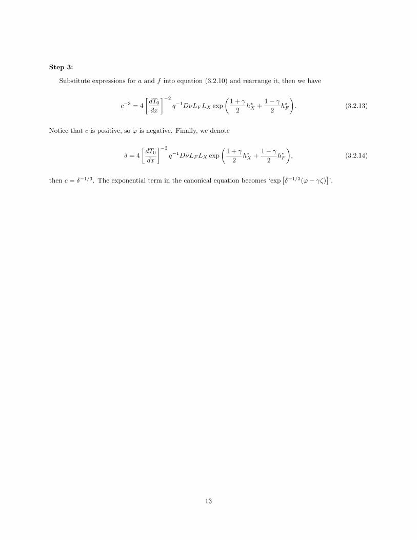
Step 3:

Substitute expressions for a and f into equation (3.2.10) and rearrange it, then we have

c−3 = 4

[dT0dx

]−2q−1DνLFLX exp

(1 + γ

2h∗X +

1− γ2

h∗F

). (3.2.13)

Notice that c is positive, so ϕ is negative. Finally, we denote

δ = 4

[dT0dx

]−2q−1DνLFLX exp

(1 + γ

2h∗X +

1− γ2

h∗F

), (3.2.14)

then c = δ−1/3. The exponential term in the canonical equation becomes ‘exp[δ−1/3(ϕ− γζ)

]’.

13

Chapter 4

Effects of Finite Distance BetweenFuel and Oxidant Supply

In this chapter, we consider a counterflow diffusion flame with plug-flow boundary conditions, in which the

exit velocity has no transverse component. The flow is therefore rotational at the reactants supply. The

schematic graph of the counterflow diffusion flames is shown in Figure 4.1.

Figure 4.1: Schematic plot of a counterflow diffusion flame.

14

4.1 Similarity Solutions for Inviscid Counterflows in Cartesian

Coordinate

If the high injection velocity at the reactant supply is high, a viscous layer will develop, separating two

inviscid regions on each side of the stagnation plane. Similarity solutions for such counterflows with plug

flow boundary conditions have been found using large Reynolds number asymptotics [26, 13]. We will adopt

the assumptions and methodology in [13, 14] and derive the velocity components in a Cartesian coordinate.

Let us assume that density and temperature are constants at both the inviscid regions. The boundary

conditions and the continuous condition at stagnation plane are

ρ = ρ0, u = u0, v = 0, x = −h, (4.1.1)

ρ = ρ1, u = u1, v = 0, x = h, (4.1.2)

u = 0, x = x0. (4.1.3)

Introduce f(x) = ρu(x) and v = −y(1/ρ)f ′(x) so that the continuity equation is satisfied. The momen-

tum equations can be reduced to

f (f/ρ)′ = −∂p∂x, (4.1.4)

f (f ′/ρ)′ − f ′ 2/ρ = k, (4.1.5)

where k is a constant, which ensure the existence of similarity solutions. It is an eigenvalue related to the

pressure, namely k = (1/y)(∂p/∂y), and it is determined by the boundary conditions as

k =π2

16h2(u0√ρ0 + u1

√ρ1)

2. (4.1.6)

By satisfying conditions (4.1.1), (4.1.2), (4.1.3), one can obtain the solution for velocity components,

pressure and the location of stagnation plane x0:

u =

u0 sin

(π

2

x0 − xx0 + h

)−h < x < x0

−u1 sin

(π

2

x0 − xx0 − h

)x0 < x < h

(4.1.7)

v =

πu0

2(x0 + h)cos

(π

2

x0 − xx0 + h

)y −h < x < x0

− πu12(x0 − h)

cos

(π

2

x0 − xx0 − h

)y x0 < x < h

(4.1.8)

15

p =

π2y2

32h2(u0√ρ0 + u1

√ρ1)2 +

ρ0u20

4cos

(πx0 − xx0 + h

)+ Const. −h < x < x0

π2y2

32h2(u0√ρ0 + u1

√ρ1)2 +

ρ1u21

4cos

(πx0 − xx0 − h

)+ Const. x0 < x < h

(4.1.9)

x0 =u0√ρ0 − u1

√ρ1

u0√ρ0 + u1

√ρ1h. (4.1.10)

The stagnation plane will locate at x = x0 when ρ0u20 = ρ1u

21.

Since the flow is rotational, it is worth looking at the vorticity as well. From equation (4.1.7) and (4.1.8),

we can get the expression for vorticity,

ωz =∂v

∂x−

����0

∂u

∂y=

π2u0

4(x0 + h)2sin

(π

2

x0 − xx0 + h

)y −h < x < x0

− π2u14(x0 − h)2

sin

(π

2

x0 − xx0 − h

)y x0 < x < h

(4.1.11)

Figure 4.2 below shows the vorticity profiles for different values of y. Vorticity have maximum values at

the reactant supply and vanish at the stagnation plane, which is fundamentally different from the case of a

potential flow. Note that this is only true when we assume constant density and at the same time ignore

the vorticity generation by viscous effects and by the flame.

20 15 10 5 0 5 10 15 20x

0.4

0.3

0.2

0.1

0.0

0.1

0.2

0.3

0.4

Vor

tici

ty ω

z

y=2

y=1

y=0

y=−1

y=−2

Figure 4.2: Vorticity profiles when u0 = u1, ρ0 = ρ1 and Ks|x=x0 = 2.

16

One of the key parameters for analysis of the flame structure is the strain rate. At the stagnation plane,

it can be calculated from equation (4.1.7) and (4.1.10) as

Ks|x=x0 = −∂u∂x

∣∣∣∣x=x0

=

πu04h

(1 +

u1√ρ1

u0√ρ0

)x = x−0

− πu14h

(1 +

u0√ρ0

u1√ρ1

)x = x+0

(4.1.12)

Compared to the case of cylindrical coordinate in [13, 14], there is a factor of (π/4) for Cartesian coordinate.

It is obvious that the strain rate at the oxidant side will equal to that at the fuel side only if ρ0 = ρ1.

4.2 Constant Density Approximation and the Diffusion Flames

Assuming that density is constant, Equation (2.2.1f) is replaced by ρ = 1, hence the velocity field and

combustion are decoupled. Taking the flame to be flat, Equation (2.2.1c), (2.2.1d) and (2.2.1e) can be

reduced to

udT

dx− d2T

dx2= 0, (4.2.1a)

udY

dx− L−1F

d2Y

dx2= 0, (4.2.1b)

udX

dx− L−1X

d2X

dx2= 0. (4.2.1c)

Boundary conditions are given as

T = 1, Y = Y0, X = 0 at x = −h

T = 1 + ∆T, Y = 0, X = X0 at x = h

Conditions at the flame x = xf are

[T ] = [Y ] = [X] = 0, (4.2.2)[dT

dx

]= − q

LF

[dY

dx

]= − q

νLX

[dX

dx

], (4.2.3)

Y |x=x+f

= β−1LFqSF (γ, δ), X|x=x−

f= β−1

νLXq

SX(γ, δ). (4.2.4)

17

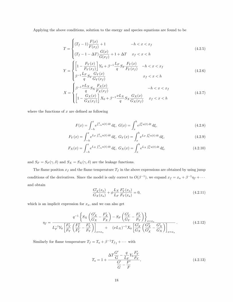
Applying the above conditions, solution to the energy and species equations are found to be

T =

(Tf − 1)

F (x)

F (xf )+ 1 −h < x < xf

(Tf − 1−∆T )G(x)

G(xf )+ 1 + ∆T xf < x < h

(4.2.5)

Y =

[1− FY (x)

FY (xf )

]Y0 + β−1

LFqSF

FY (x)

FY (xf )−h < x < xf

β−1LFqSF

GY (x)

GY (xf )xf < x < h

(4.2.6)

X =

β−1

νLXq

SXFX(x)

FX(xf )−h < x < xf[

1− GX(x)

GX(xf )

]X0 + β−1

νLXq

SXGX(x)

GX(xf )xf < x < h

(4.2.7)

where the functions of x are defined as following

F (x) =

∫ x

−he∫ ξ−hu(t) dt dξ, G(x) =

∫ h

x

e∫ ξhu(t) dt dξ, (4.2.8)

FY (x) =

∫ x

−heLF

∫ ξ−hu(t) dt dξ, GY (x) =

∫ h

x

eLF∫ ξhu(t) dt dξ, (4.2.9)

FX(x) =

∫ x

−heLX

∫ ξ−hu(t) dt dξ, GX(x) =

∫ h

x

eLX∫ ξhu(t) dt dξ, (4.2.10)

and SF = SF (γ, δ) and SX = SX(γ, δ) are the leakage functions.

The flame position xf and the flame temperature Tf in the above expressions are obtained by using jump

conditions of the derivatives. Since the model is only correct to O(β−1), we expand xf = xa + β−1ηf + · · ·

and obtain

G′X(xa)

GX(xa)+ φ

LXLF

F ′Y (xa)

FY (xa)= 0, (4.2.11)

which is an implicit expression for xa, and we can also get

ηf =

q−1{SX

(G′XGX− F ′XFX

)− SF

(G′YGY− F ′YFY

)}x=xa

L−1F Y0

[F ′YFY

(F ′′YF ′Y− F ′YFY

)]x=xa

+ (νLX)−1X0

[G′XGX

(G′′XG′X− G′XGX

)]x=xa

. (4.2.12)

Similarly for flame temperature Tf = Ta + β−1Tf 1 + · · · with

Ta = 1 +∆T

G′

G− q

LFY0F ′YFY

G′

G− F ′

F

, (4.2.13)

18

and

Tf 1 =

(G′

G− F ′

F

)−1{− q

LFY0F ′YFY

(F ′′YF ′Y− F ′YFY

)ηf − SF

(G′YGY− F ′YFY

)−(Ta − 1−∆T )

G′

G

(G′′

G′− G′

G

)ηf + (Ta − 1)

F ′

F

(F ′′

F ′− F ′

F

)ηf

}. (4.2.14)

All the functions F , G, FX , GX , FY , GY and their derivatives in Equation (4.2.12), (4.2.13) and (4.2.14)

are evaluated at x = xa.

4.3 The Burke-Schumann Limit Solution

If the reaction is infinitely fast and all the reactants are consumed right at the flame, often termed as the

Burke-Schumann limit, the reaction zone reduces to a surface x = xa. All the O(β−1) terms in (4.2.5),

(4.2.6) and (4.2.7) are neglected in this limit. An example of temperature profile and mass fractions of fuel

and oxidant is given in Figure 4.3. The boundary conditions are set to be the same with the experiment

in [27] for a n-Heptane counterflow diffusion flame: T0 = 338 K, T1 = 298 K, U0 = 34.2 cm/s, U1 = 37.5

cm/s, Y0 = 0.3866 and X0 = 0.233. Separation distance of the burner is 10 mm. The Burke-Schmann limit

solution returned a flame temperature above 2400 K, which is much higher than the results in [27], 1767 K in

computation and a corrected measured value of 1730 K. This implies that the effects of finite reaction rates

are significant especially when the the strain rate is high and the flame is close to extinction. By including

the O(β−1) terms in (4.2.5), (4.2.6) and (4.2.7), we would expect to have a better agreement with [27].

We can obtain the flame location to the leading order by solving equation (4.2.11). Figure 4.4 shows how

it varies with the mixture strength φ. When we match the stain rate at the stagnation plane of a plug flow

with that of a potential flow, we will have the same flame location for both cases. This is because the flame

stays close to the stagnation plane and it is subjected to nearly the same strain rate, as shown in Figure

4.5. At the stagnation plane, Ks = 2, while at the flame, Ks only deviates less than 0.2% for 0.3 < φ < 4.5.

Therefore the characteristic strain rate ε introduced in the non-dimensionalization can be chosen as the

strain rate at the stagnation plane. However, this is good only under constant density assumption. Thermal

expansion, which will be discussed in the next chapter, will alert the stain rate at the flame.

The flame locations are plotted for different Lewis numbers LF , LX in Figure 4.6, and for different

velocity ratio u1/u0 in Figure 4.7. By comparing Figure 4.6 with Figure 4.4, one can observe that the

mixture strength has a stronger influence on the flame location than the Lewis numbers. The velocity ratio

is even more important in determining where the flame is, as shown in Figure 4.7.

19

0.00

0.05

0.10

0.15

0.20

0.25

0.30

0.35

0.40

Mas

s Fr

acti

ons

Y an

d X Y (Fuel)

X (Oxidizer)

0.2 0.3 0.4 0.5 0.6 0.7 0.8Distance from Fuel Supply [cm]

0

500

1000

1500

2000

2500

Tem

pera

ture

[K

]

Figure 4.3: Temperature profile and mass fractions of fuel and oxidant when T0 = 338 K, T1 = 298 K,U0 = 34.2 cm/s, U1 = 37.5 cm/s, Y0 = 0.3866, X0 = 0.233. Separation distance of the reactant supplies is1cm.

20

0 1 2 3 4 5φ

0.6

0.4

0.2

0.0

0.2

0.4

0.6

0.8

xa

Plug FlowPotential Flow

Figure 4.4: Flame location xa for different values of φ when u0 = u1 and LF = LX = 1. Comparisons fordifferent boundary conditions are given when strain rates at the stagnation plane for both cases are the sameand Ks|x=x0

= 2.

21

0 1 2 3 4φ

1.94

1.96

1.98

2.00

2.02

2.04

2.06Fl

ame

Stre

tch

LF =LX =1

LF =0.8, LX =1

LF =1.6, LX =1

Figure 4.5: Flame Stretch K for different values of φ when u0 = u1.

22

0.4 0.6 0.8 1.0 1.2 1.4 1.6 1.8 2.0Lewis Number LF or LX

0.20

0.15

0.10

0.05

0.00

0.05

0.10

0.15

0.20xa

xa v.s. LX , LF =1

xa v.s. LF , LX =1

Figure 4.6: Flame location xa for different values of LF and LX when u0 = u1, φ = 1 and Ks|x=x0= 2. The

flame move towards more diffusive species.

0.4 0.6 0.8 1.0 1.2 1.4 1.6 1.8 2.0u1 /u0

8

6

4

2

0

2

4

6

8

xa

φ=0.5

φ=1.0

φ=2.0

Figure 4.7: Flame location xa for different values of u1/u0 when LF = LX = 1 and Ks|x=x0= 2. Note that

when φ = 1, the flame collocates at the stagnation plane.

23

4.4 Flame Behaviors near Extinction

For finite chemical reaction rate, in which case the Damkohler number is no longer infinite, there exists

reactant leakage through the flame sheet. The leakage increases with injection velocities of the reactant,

which results in a smaller heat release and hence a lower flame temperature. At a certain critical point,

extinction will happen due to insufficient heat release from the chemical reactions to sustain the combustion

process.

According to the constant density solution (4.2.5), the parameter γ and δ takes the form of

γ =

(Ta − 1)

[G′

G+F ′

F

]−∆T

G′

G

(Ta − 1)

[G′

G− F ′

F

]−∆T

G′

G

, (4.4.1)

δ =

4νLFLXD exp

{(Tf − Ta)β +

1 + γ

2SX +

1− γ2

SF

}q

[(Ta − 1)

[G′

G− F ′

F

]−∆T

G′

G

]2 . (4.4.2)

where functions F , G and their derivatives are evaluated at x = xa.

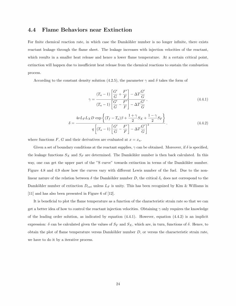
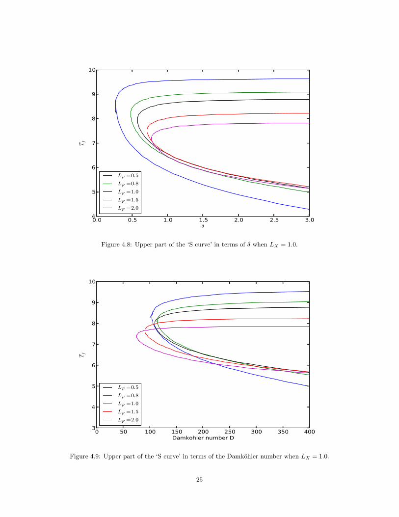
Given a set of boundary conditions at the reactant supplies, γ can be obtained. Moreover, if δ is specified,

the leakage functions SX and SF are determined. The Damkohler number is then back calculated. In this

way, one can get the upper part of the ”S curve” towards extinction in terms of the Damkohler number.

Figure 4.8 and 4.9 show how the curves vary with different Lewis number of the fuel. Due to the non-

linear nature of the relation between δ the Damkohler number D, the critical δc does not correspond to the

Damkohler number of extinction Dext unless LF is unity. This has been recognized by Kim & Williams in

[11] and has also been presented in Figure 6 of [12].

It is beneficial to plot the flame temperature as a function of the characteristic strain rate so that we can

get a better idea of how to control the reactant injection velocities. Obtaining γ only requires the knowledge

of the leading order solution, as indicated by equation (4.4.1). However, equation (4.4.2) is an implicit

expression: δ can be calculated given the values of SF and SX , which are, in turn, functions of δ. Hence, to

obtain the plot of flame temperature versus Damkohler number D, or versus the characteristic strain rate,

we have to do it by a iterative process.

24

0.0 0.5 1.0 1.5 2.0 2.5 3.0δ

4

5

6

7

8

9

10

Tf

LF =0.5

LF =0.8

LF =1.0

LF =1.5

LF =2.0

Figure 4.8: Upper part of the ‘S curve’ in terms of δ when LX = 1.0.

0 50 100 150 200 250 300 350 400Damkohler number D

3

4

5

6

7

8

9

10

Tf

LF =0.5

LF =0.8

LF =1.0

LF =1.5

LF =2.0

Figure 4.9: Upper part of the ‘S curve’ in terms of the Damkohler number when LX = 1.0.

25

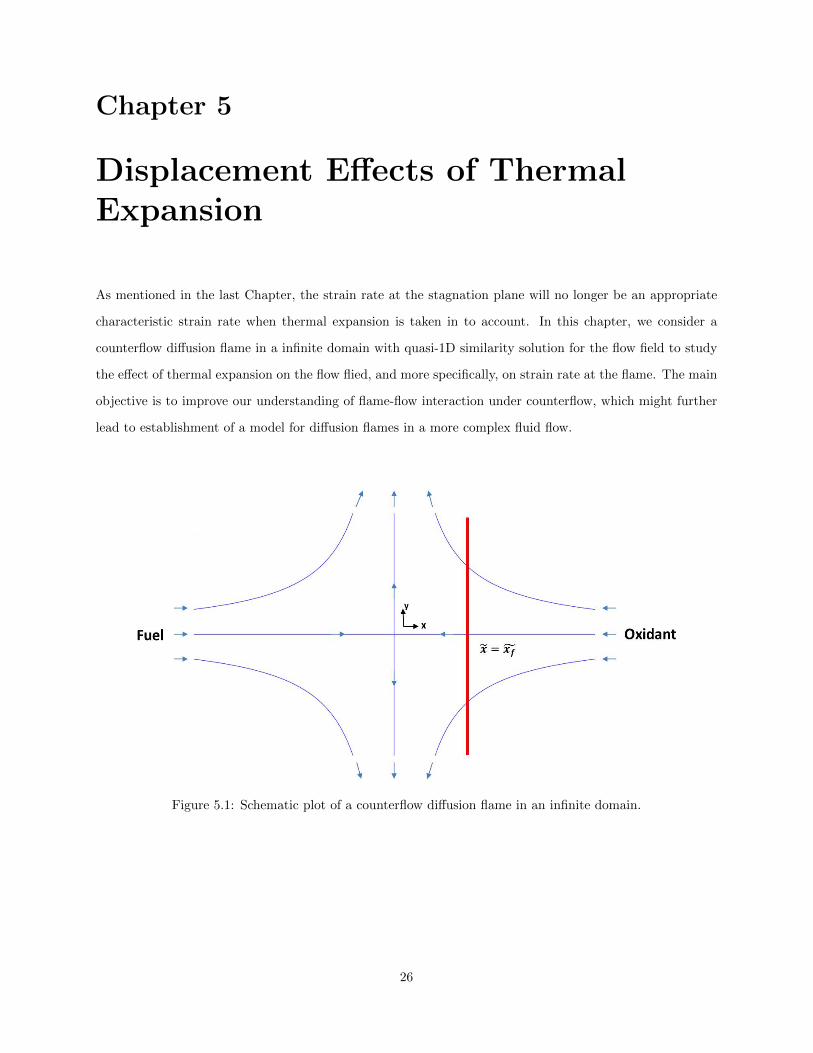
Chapter 5

Displacement Effects of ThermalExpansion

As mentioned in the last Chapter, the strain rate at the stagnation plane will no longer be an appropriate

characteristic strain rate when thermal expansion is taken in to account. In this chapter, we consider a

counterflow diffusion flame in a infinite domain with quasi-1D similarity solution for the flow field to study

the effect of thermal expansion on the flow flied, and more specifically, on strain rate at the flame. The main

objective is to improve our understanding of flame-flow interaction under counterflow, which might further

lead to establishment of a model for diffusion flames in a more complex fluid flow.

Figure 5.1: Schematic plot of a counterflow diffusion flame in an infinite domain.

26

5.1 Formulation of the Numerical Problem

The schematic plot of a flat counterflow diffusion flame in an infinite domain is shown in Figure 5.1. By

assuming

u = u(x), v = y V (x), (5.1.1)

the governing equations in Chapter 2 can be reduced to a system of non-linear ODEs,

(ρu)x + ρV = 0, (5.1.2)

ρuux = −px + Pr

[4

3uxx −

1

3Vx

], (5.1.3)

ρuVx + ρV 2 = ρ0ε20 + PrVxx, (5.1.4)

ρuTx − Txx = qω, (5.1.5)

ρuYx − L−1F Yxx = −ω, (5.1.6)

ρuXx − L−1X Xxx = −νω, (5.1.7)

ρT = 1. (5.1.8)

Boundary conditions are given as

V = −ε0, T = T0 = 1, Y = Y0, X = 0 at x = −∞

V = −ε1, T = T1, Y = 0, X = X1 at x =∞

and u = 0 at x = 0

The above conditions must satisfy the requirement for quasi-1D similarity solution

−1

y

∂p

∂y= Const. (5.1.9)

To satisfy the boundary conditions, we enforce

−1

y

∂p

∂y= ρ1ε

21 = ρ0ε

20, (5.1.10)

or equivalently T0/T1 = ε20/ε21.

27

5.2 Numerical Methods

The above systems of non-linear ODEs is solved by pseudo-transient formulation, which starts from a

desirable and physical analytical solution and gradually approaches the steady-state solution. The pseudo-

transient terms are discretized by forward Euler difference while derivatives with respect to x are discretized

by second order central difference. Newton’s method with a well-defined analytical Jacobian is used in the

MATLAB code. Trust-redion dogleg algorithm is applied in the iterations.

Initial condition can be obtained in two ways, either a analytical solution or a previous numerical solution

that is close to the desired steady state solution. If the Lewis numbers are unity, LF = LX = 1, one can

obtain the analytical solutions in the Burke-Schumann limit, as listed in Page 75 of [28]. If we have already

obtained some steady-state numerical solutions from the code and we want to get other solutions with

different parameters, we can also start with the previous numerical results.

The transient momentum equation in x direction is in the form of a wave equation,

∂ρu

∂t+∂f(v, ρ, p)

∂x= 0, (5.2.1)

so the information of it will propagate to either positive or negative direction in x. As a result, forcing the

transverse velocity u to be zero at the origin will give rise to fluctuation in u in one side of the computational

domain. Since the system of equations is invariant in x axis, we can assign the velocity at the left boundary

of the computational domain to satisfy the boundary conditions while avoiding fluctuation in u. After the

computation is finished the stagnation plane will be shifted back to the origin.

In our computation, the strain rates of the incoming potential flow are ε0 = ε1 = 2, so temperatures at

the boundaries must be the same. The controlling parameter for thermal expansion is the density ratio σ,

defined as σ = ρ0/ρa, or

σ =Ta

T0=Q/WF νF

cpT0

Y01 + φ

(5.2.2)

A larger sigma represents more heat release. After σ is chosen, heat release Q is then calculated and fed

into the computation as an input parameter. The limit σ = 1 stands for the constant density assumption,

which is consistent with the analytical initial solution.

To interpolate the stain rate at the flame sheet, we need the location of the flame sheet first. Taylor

expansion of the temperature, instead of reaction rate, at the flame is used for the stability when taking

28

derivatives numerically. If the temperature is assumed to peak at the flame sheet, then

∂T

∂x

∣∣∣∣x=xf

=∂T

∂x

∣∣∣∣x=xN+dxf

= 0 (5.2.3)

where xN is the grid point right in front of xf , so xN < xf < xN+1. xN and xN+1 can be found by

searching for neighboring grid points on which we have the largest two temperature values. Expanding the

temperature derivative at the flame, we have

∂T

∂x

∣∣∣∣x=xN

+ dxf∂2T

∂x2

∣∣∣∣x=xN

+O(dx2f ) = 0. (5.2.4)

We can approximate the above derivatives numerically by second order central difference,

∂T

∂x

∣∣∣∣x=xN

=T (xN+1)− T (xN−1)

2∆x+O(∆x2), (5.2.5)

∂2T

∂x2

∣∣∣∣x=xN

=T (xN+1)− 2T (xN ) + T (xN−1)

∆x2+O(∆x2). (5.2.6)

Therefore, the flame location can be obtained by

xf = xN −T (xN+1)− T (xN−1)

T (xN+1)− 2T (xN ) + T (xN−1)

∆x

2. (5.2.7)

5.3 Displacement Effects of the Flame

The standoff distances of the flow are defined such that the far field transverse velocity component can be

express as

u ∼ −ε0(x+ ∆xF ), x→ −∞ and u ∼ −ε1(x−∆xO), x→ +∞. (5.3.1)

Figure 5.2 illustrates the definition above. Due to thermal expansion, the flame acts as if it pushes the

incoming potential flow back by ∆xF for the fuel side and ∆xO for the oxidant side.

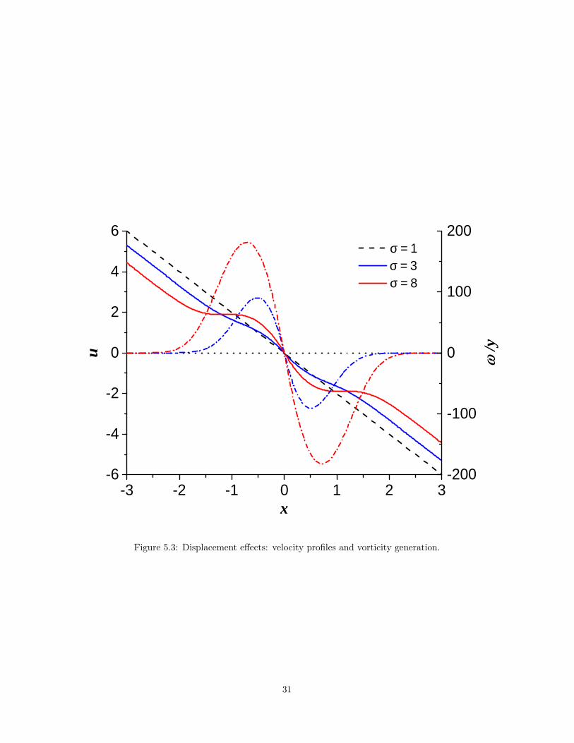
Numerical solutions of the transverse velocity u when φ = 1 and LF = LX = 1 is plotted in Figure 5.3.

The flame locates right at the stagnation plane x = x0. The flow near the flame is accelerated due to thermal

expansion, hence the strain rate at the flame is increased. The flame can be regarded as a source of vorticity,

which increases linearly in y in our formulation. Hence, we can plot the quantity ω/y (y 6= 0) to study the

vorticity generation. From Figure 5.3, one can conclude that the vorticity generated by the flame increases

with the density ratio σ, and it vanishes upstream so that the far field incoming flow remains irrotational.

29

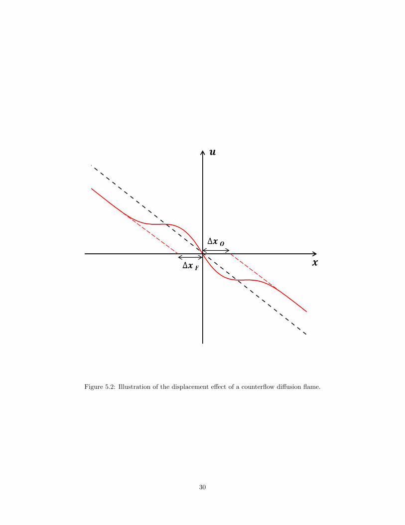
Figure 5.2: Illustration of the displacement effect of a counterflow diffusion flame.

30

- 3 - 2 - 1 0 1 2 3- 6

- 4

- 2

0

2

4

6

u

σ = 1 σ = 3 σ = 8

x- 2 0 0

- 1 0 0

0

1 0 0

2 0 0

��/y

Figure 5.3: Displacement effects: velocity profiles and vorticity generation.

31

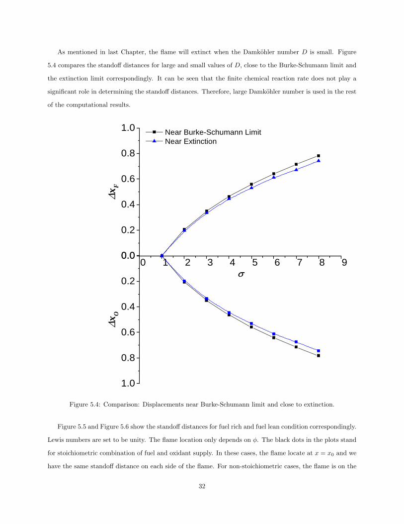
As mentioned in last Chapter, the flame will extinct when the Damkohler number D is small. Figure

5.4 compares the standoff distances for large and small values of D, close to the Burke-Schumann limit and

the extinction limit correspondingly. It can be seen that the finite chemical reaction rate does not play a

significant role in determining the standoff distances. Therefore, large Damkohler number is used in the rest

of the computational results.

0 1 2 3 4 5 6 7 8 90 . 0

0 . 2

0 . 4

0 . 6

0 . 8

1 . 0 N e a r B u r k e - S c h u m a n n L i m i t N e a r E x t i n c t i o n

�xF

�

1 . 0

0 . 8

0 . 6

0 . 4

0 . 2

0 . 0

�xO

Figure 5.4: Comparison: Displacements near Burke-Schumann limit and close to extinction.

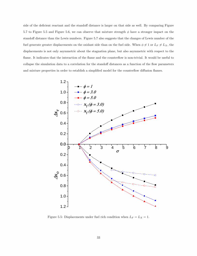
Figure 5.5 and Figure 5.6 show the standoff distances for fuel rich and fuel lean condition correspondingly.

Lewis numbers are set to be unity. The flame location only depends on φ. The black dots in the plots stand

for stoichiometric combination of fuel and oxidant supply. In these cases, the flame locate at x = x0 and we

have the same standoff distance on each side of the flame. For non-stoichiometric cases, the flame is on the

32

side of the deficient reactant and the standoff distance is larger on that side as well. By comparing Figure

5.7 to Figure 5.5 and Figure 5.6, we can observe that mixture strength φ have a stronger impact on the

standoff distance than the Lewis numbers. Figure 5.7 also suggests that the changes of Lewis number of the

fuel generate greater displacements on the oxidant side than on the fuel side. When φ 6= 1 or LF 6= LX , the

displacements is not only asymmetric about the stagnation plane, but also asymmetric with respect to the

flame. It indicates that the interaction of the flame and the counterflow is non-trivial. It would be useful to

collapse the simulation data to a correlation for the standoff distances as a function of the flow parameters

and mixture properties in order to establish a simplified model for the counterflow diffusion flames.

0 1 2 3 4 5 6 7 8 90 . 0

0 . 2

0 . 4

0 . 6

0 . 8

1 . 0

1 . 2 � � � � � � � � � � � � � � � � � � �

�xF

�

1 . 2

1 . 0

0 . 8

0 . 6

0 . 4

0 . 2

0 . 0

x f � � � � � � � � �

x f � � � � � � � � �

�xO

Figure 5.5: Displacements under fuel rich condition when LF = LX = 1.

33

0 1 2 3 4 5 6 7 8 90 . 0

0 . 2

0 . 4

0 . 6

0 . 8

1 . 0

1 . 2 � � � � � � � � � � � � � � � � � � � x f � � � � � � � � �

x f � � � � � � � � � �

�xF

�

1 . 2

1 . 0

0 . 8

0 . 6

0 . 4

0 . 2

0 . 0

�xO

Figure 5.6: Displacements under fuel lean condition when LF = LX = 1.

34

0 1 2 3 4 5 6 7 8 90 . 0

0 . 3

0 . 6

0 . 9 L e F = 1 . 0 L e F = 0 . 8 L e F = 1 . 5

x f � L e f � � � � � � �

�xF

�

0 . 9

0 . 6

0 . 3

0 . 0

x f � L e f � � � � � � ��x

O

Figure 5.7: Displacements for different values of LF when LX = 1 and φ = 1.

Instead of introducing the standoff distances, we can define a length scale based on vorticity generation

to quantify the displacement effects of the diffusion flame. Let’s define a ’1% voricity layer’ as the region

where we have more than 1% of the maximum magnitude of ω/y (y 6= 0) generated by the flame. Therefore

the incoming potential flow out side of this layer remains irrotatoinal and does not ’feel’ the existence of the

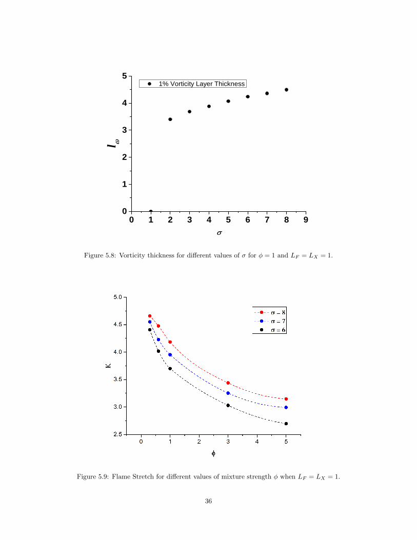
flame. Figure 5.8 shows how the thickness of ’1% voricity layer’ changes with density ratio σ. An increase

in σ, or an increase in heat release, will result in a thicker vorticity layer.

35

0 1 2 3 4 5 6 7 8 90

1

2

3

4

5 1 % V o r t i c i t y L a y e r T h i c k n e s s

l �

�

Figure 5.8: Vorticity thickness for different values of σ for φ = 1 and LF = LX = 1.

Figure 5.9: Flame Stretch for different values of mixture strength φ when LF = LX = 1.

36

As shown in Figure 4.5, the flow near the flame is accelerated, which gives rise to an increased strain

rate compared to the strain rate of the incoming potential flow. Since the above analysis indicates that φ

is the most influential parameter for the displacement effects, we choose to plot the the strain rate at the

flame, which is also the flame stretch in this case, versus the mixture strength φ. The strain rate at the

computational boundary is K = 2, while thermal expansion can increase this value by more than 100% for

certain values of φ and σ. Therefore, when we choose the characteristic stain rate to analyze extinction

phenomena, we have to consider the acceleration effects of thermal expansion. For large φ, Kim & Williams

[29] has proposed a correction factor to account for the variable density effects. However, Figure 4.5 suggests

that the increase in strain rate is more significant in under fuel lean combustion. Considering also that lean

combustion is of more and more interest for environmental concerns, a correction factor for small φ or for

more general cases is of practical values.

37

Chapter 6

Slightly Curved Counterflow DiffusionFlames

In the previous Chapters, the discussions on counterflow diffusion flames was based on the quasi-1D formu-

lation, which requires the eigenvalue Λ = (1/y)(∂p/∂y) to be a constant. However, this requirement is not

always satisfied, especially for burners with a converging small diameter nozzle [20, 21]. The attempt here

is to extend our knowledge of the quasi-1D theory and introduce a potential flow that will allow variations

of Λ and that will support a slowly varying counterflow flame. This might shed light on the mathematical

description of a 2D curved counterflow flame and the results could serve as an initial condition for a full

numerical simulation in the future work.

6.1 Governing Equations in 2D

The dimensionless governing equations in 2D are

(ρu)x + (ρv)y = 0 (6.1.1)

ρ (uux + vuy) = −px + Pr∇2u (6.1.2)

ρ (uvx + vvy) = −py + Pr∇2v (6.1.3)

ρ (uTx + vTy) = qω +∇2T (6.1.4)

ρ (uYx + vYy) = −ω + L−1F ∇2Y (6.1.5)

ρ (uXx + vXy) = −νω + L−1X ∇2X (6.1.6)

ρT = 1 (6.1.7)

The subscripts denote derivatives with respect to x and y. In the momentum equation, p is the modified

pressure. The dimensionless chemical reaction rate ω of one-step reaction is given in Chapter 1.

38

6.2 Review of the Quasi-One-Dimensional Theory

The schematic plot of a flat counterflow flame has previously been shown in Figure 5.1. By assuming

ρu = f(x) and ρv = −yf ′(x), (6.2.1)

the continuity equation is satisfied. Then momentum equations can be reduced to

f(fT )x − Pr(fT )xx = −px, (6.2.2)

−f(fxT )x + f2xT + Pr(fxT )xx = −1

ypy. (6.2.3)

Boundary conditions are given as

vy = ε0, T = 1, Y = Yu, X = 0 as x→ −∞

vy = ε1, T = T1, Y = 0, X = Xu as x→∞

and u = 0 at x = 0

For one-dimensional similarity solution to exist, we must have

−1

y

∂p

∂y= Const. , (6.2.4)

which is a consequence of the similarity assumptions (6.2.1). By satisfying the boundary conditions, one can

obtain the eigenvalue

Λ = (1/y)(∂p/∂y) = ρ0ε20 = ρ1ε

21. (6.2.5)

If the boundary conditions are changed such that the eigenvalue Λ is no longer a constant, it is possible to

create a flow pattern which support a two-dimensional curved flame. In the next section, we will introduce

such a flow and try to address the two-dimensional problem analytically.

39

6.3 Slightly Curved Flame under Constant Density Assumption

In this section, a potential flow is considered in order to obtain a curved counterflow diffusion flame with

constant density assumption. The velocity components are

u = −2x+ β (x2 − y2), (6.3.1)

v = 2y − β (2xy), (6.3.2)

where β � 1. Note that the β here is a small parameter for the flow field and is different from the large

activation energy parameter introduced in Chapter 1. When β → 1, we will get the potential flow often used

in quasi-1D theory. By Bernoulli’s equation, pressure can be calculated as

p = −2(x2 + y2) + β[2x(x2 + y2)

]− β2

[1

2(x2 + y2)2

]. (6.3.3)

And the eigenvalue Λ = (1/y)(∂p/∂y) is therefore

Λ = −4 + 4β x− β2[2(x2 + y2)

], (6.3.4)

which is no longer a constant. Plots of streamlines, pressure contours and the eigenvalue Λ are shown in

Figure 6.1, Figure 6.2 and Figure 6.3. As β increases, the flow become more asymmetric about y axis.

(a) β = 0.3 (b) β = 0.5

Figure 6.1: Streamlines of the potential counterflows

40

Assuming LF = LX = L , we can construct a conserved scalar H = ν−1X − Y , the governing equation

of which is

uHx + v Hy −L −1 (Hxx +Hyy) = 0 (6.3.5)

with boundary conditions

H ∼ −Yu, x→ −∞ (6.3.6)

H ∼ ν−1Xu, x→ +∞ (6.3.7)

Suppose that the flame is varying slowly in y and ε is the small parameter for curvature of the flame. The

flame front is determined by equation H(x, εy) = 0. Let η = εy, we can expand H(x, η) into an asymptotic

series

H(x, η) ∼ H0(x) + εH1(x, η) +O(ε2) (6.3.8)

The velocity components can be written as

u(x, η) = −2x− β

ε2η2 + βx2 (6.3.9)

v(x, η) =1

ε(2η − 2βxη) (6.3.10)

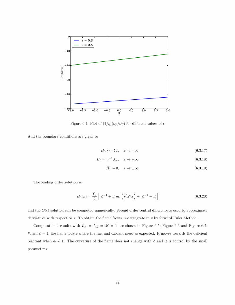
To have the flat flame solution to the leading order we must have β/ε2 � 1. Take β = ε3 and we have

u(x, η) = −2x− εη2 + ε3x2 (6.3.11)

v(x, η) =1

ε

(2η − 2ε3xη

)(6.3.12)

p(x, η) = − 2

ε2η2 − 2x2 + 2εxη2 (6.3.13)

(1/η)(∂p/∂η) = − 4

ε2+ 4εx (6.3.14)

Note that (1/η)(∂p/∂η) varies linearly in x, as shown in Figure 6.4, and it does not depend on y.

Governing equations for the conserved scalar to the leading order and O(ε) are

2xH0x + L −1H0xx = 0 (6.3.15)

2xH1x − 2ηH1η + L −1H1xx = −η2 2√π

e−x2

(6.3.16)

41

(a) β = 0.3

(b) β = 0.5

Figure 6.2: Contour plots of pressure

42

2.0 1.5 1.0 0.5 0.0 0.5 1.0 1.5 2.0x

8

7

6

5

4

3

2Λ

y = 2.0y = 1.0y = 0y = -1.0y = -2.0

(a) β = 0.3

2.0 1.5 1.0 0.5 0.0 0.5 1.0 1.5 2.0x

12

10

8

6

4

2

Λ

y = 2.0y = 1.0y = 0y = -1.0y = -2.0

(b) β = 0.5

Figure 6.3: Plots of Eigenvalue Λ = (1/y)(∂p/∂y)

43

2.0 1.5 1.0 0.5 0.0 0.5 1.0 1.5 2.0x

50

40

30

20

10

0

(1/η

)(p/

η)

ε = 0.3

ε = 0.5

Figure 6.4: Plot of (1/η)(∂p/∂η) for different values of ε

And the boundary conditions are given by

H0 ∼ −Yu, x→ −∞ (6.3.17)

H0 ∼ ν−1Xu, x→ +∞ (6.3.18)

H1 ∼ 0, x→ ±∞ (6.3.19)

The leading order solution is

H0(x) =Yu2

[(φ−1 + 1) erf

(√L x

)+ (φ−1 − 1)

](6.3.20)

and the O(ε) solution can be computed numerically. Second order central difference is used to approximate

derivatives with respect to x. To obtain the flame fronts, we integrate in y by forward Euler Method.

Computational results with LF = LX = L = 1 are shown in Figure 6.5, Figure 6.6 and Figure 6.7.

When φ = 1, the flame locate where the fuel and oxidant meet as expected. It moves towards the deficient

reactant when φ 6= 1. The curvature of the flame does not change with φ and it is control by the small

parameter ε.

44

2.0 1.5 1.0 0.5 0.0 0.5 1.0 1.5 2.0x

2.0

1.5

1.0

0.5

0.0

0.5

1.0

1.5

2.0

η

Figure 6.5: Plot of streamlines and the flame front when φ = 1.0

2.0 1.5 1.0 0.5 0.0 0.5 1.0 1.5 2.0x

2.0

1.5

1.0

0.5

0.0

0.5

1.0

1.5

2.0

η

Figure 6.6: Plot of streamlines and the flame front when φ = 3.0

45

2.0 1.5 1.0 0.5 0.0 0.5 1.0 1.5 2.0x

2.0

1.5

1.0

0.5

0.0

0.5

1.0

1.5

2.0

η

Figure 6.7: Plot of streamlines and the flame front when φ = 0.4

Going from constant density examples to variable density simulations is non-trivial. We need to consider

thermal expansion effects on the flow. One of the most difficult part is to assign proper boundary conditions

so that the far field incoming counterflow behaves like the potential flow we proposed here. Although

the problem can be parabolized by taking the ”slowly varying flame” assumption, we still need to derive

boundary condtions for pressure in the limit |y| → ∞ because either the pressure Poisson equation or the

vorticity-streamfunction relation is elliptic. A more interesting study would be numerical simulations of a

two dimensional curved flame without assuming that the flame varies slowly in y.

46

Chapter 7

Conclusions and Future Works

Counterflow diffusion flames with one-step global reaction are studied using asymptotic theories and numer-

ical techniques. The general asymptotic theory for multi-dimensional diffusion flames with non unity Lewis

numbers and large activation energy reactions [12] is revised and the derivation of the canonical equation

is given in detail. The theory is then applied to a counterlfow configuration with plug flow boundary con-

ditions. By assuming that density is constant, asymptotic solutions for the flames with non-unity Lewis

numbers and finite rate chemistry are found. From the leading order results, we can conclude that the strain

rate at the flame is close to the strain rate at the stagnation plane in the constant density limit. Hence,

plug flow boundary conditions are observed to have the same flame location as the potential flow boundary

conditions, when the strain rates at the stagnation plane. for both cases are matched and the Lewis numbers

of fuel and oxidant are equal. The velocity ratio of the incoming flows at the boundary will be a dominant

parameter that control the flame location while the mixture strength φ and Lewis numbers will play minor

roles. Extinction phenomena is then studied in a quasi-steady sense. Using the leakage functions given in

[12], we can generate the upper part of the ‘S-curve’ which gives the Damkohler number at extinction Dext.

It can be used to calculate the characteristic strain rate εc, which might be chosen as the strain rate at the

stagnation plane, as an approximation of the strain rate at the flame under the constant density assumption.

Note that the expression of δ in equation (3.1.12) is implicit, so it requires iterative process to obtain δ

for a specific plug flow boundary condition. It would be useful to go through the iterations under different

plug flow boundary conditions and interpolate the results so that we can relate δ with the incoming flow

parameters explicitly.

When we include variable-density effects, the above statements under constant density assumption need

to be adjusted. Diffusion flames will have displacement effects on the incoming flows, which accelerate the

flow near the flame and hence increase the strain rate experienced by the flame [17]. By simulating one-

dimensional counterflow diffusion flames with potential flow boundary conditions, the displacement effects

of the flames are found to be stronger as the heat release increases. Under non-stoichiometric conditions,

the standoff distances are different for the fuel side and the oxidant side. It is not symmetric neither about

47

the stagnation plane nor about the flame. It is also found that the change in the Lewis number of the fuel,

no matter the increase or decrease of it, will result in a more significant displacement on the oxidant side

that on the fuel side. This is particularly interesting when LF > 1: although the flame locates on the fuel

side, the displacement effect is more obvious on the oxidant side. The strain rate at the flame is considerably

larger than that of the incoming flows, especially for flames in fuel lean conditions.

Beyond the simulations with equal strain rates at the boundaries, we can extend our knowledge to

unequal strain rates cases. The one-dimensional formulation requires that an eigenvalue Λ = (1/y)(∂p/∂y)

is a constant, or equivalently T0/T1 = ε20/ε21, so unequal strain rates at the boundary implies different

temperatures at reactant supplies. Results of these simulations will be more general and more comparable

to experiments since we could have different strain rates on the fuel side and oxidant side in practice.

By introducing a potential flow that has the eigenvalue Λ no longer a constant, we are able to create

a two-dimension counterflow diffusion flame. To address the problem analytically, several assumptions are

made, namely constant density, equal Lewis numbers for the fuel and oxidant and slowly varying flame.

Asymptotic solutions of the flame front are obtained for different values of mixture strength φ. This will be

the first step towards a multi-dimensional counterflow diffusion flame. Full numerical simulations might be

carried out in the future without the restrictive assumptions, such as slowly varying flames. This will help

us improve our understandings of the interactions between the flow and the diffusion flames.

48

References

[1] A. E. Potter Jr. and J. N. Butler, “A Novel Combustion Measurement Based on the Extinguishment ofDiffusion Flames,” ARS Journal, vol. 29, no. 1, pp. 54–56, 1959.

[2] A. E. Potter Jr., S. Heimel, and J. N. Butler, “Apparent flame strength. A measure of maximumreaction rate in diffusion flames,” in Eighth Symposium (International) on Combustion, (Pittsburgh),pp. 1027–1034, The Combustion Institute, 1962.

[3] T. P. Pandya and F. J. Weinberg, “The Structure of Flat, Counter-Flow Diffusion Flames,” Proceedingsof the Royal Society A: Mathematical, Physical and Engineering Sciences, vol. 279, no. 1379, pp. 544–561, 1964.

[4] H. Tsuji and I. Yamaoka, “The Counterflow Diffusion Flames in the Forward Stagnation Region of aPorous Cylinder,” in Twelfth Symposium (International) on Combustion, (Pittsburgh), pp. 997–1005,The Combustion Institute, 1969.

[5] H. Tsuji and I. Yamaoka, “Structure analysis of counterflow diffusion flames in the forward stagna-tion region of a porous cylinder,” in Symposium (International) on Combustion, vol. 13, (Pittsburgh),pp. 723–731, The Combustion Institute, 1971.

[6] J. Kent and F. A. Williams, “Extinction of laminar diffusion flames for liquid fuels,” in FifteenthSymposium (International) on Combustion, (Pittsburgh), pp. 315–325, The Combustion Institute, 1975.

[7] N. Peters, “Laminar diffusion flamelet models in non-premixed turbulent combustion,” Progress inEnergy and Combustion Science, vol. 10, no. 3, pp. 319–339, 1984.

[8] A. Linan, “The assymtotic structure of counterflow diffusion flames for large activation energies,” ActaAstronautica, vol. 1, pp. 1007–1039, 1974.

[9] S. Chung and C. Law, “Structure and extinction of convective diffusion flames with general Lewisnumbers,” Combustion and Flame, vol. 52, pp. 59–79, 1983.

[10] K. Seshadri and C. Trevino, “The Influence of the Lewis Numbers of the Reactants on the AsymptoticStructure of Counterflow and Stagnant Diffusion Flames,” Combustion Science and Technology, vol. 64,no. 4-6, pp. 243–261, 1989.

[11] J. S. Kim and F. A. Williams, “Extinction of diffusion flames with nonunity Lewis numbers,” Journalof engineering mathematics, vol. 31, pp. 101–118, 1997.

[12] S. Cheatham and M. Matalon, “A general asymptotic theory of diffusion flames with application tocellular instability,” Journal of Fluid Mechanics, vol. 414, pp. 105–144, 2000.

[13] K. Seshadri and F. A. Williams, “Laminar flow between parallel plates with injection of a reactant athigh reynolds number,” International Journal of Heat and Mass Transfer, vol. 21, no. 2, pp. 251–253,1978.

[14] U. Niemann, K. Seshadri, and F. A. Williams, “Accuracies of laminar counterflow flame experiments,”Combustion and Flame, vol. 162, no. 4, pp. 1540–1549, 2014.

49

[15] H. K. Chelliah, C. K. Law, T. Ueda, M. D. Smooke, and F. A. Williams, “An experimental andtheoretical investigation of the dilution, pressure and flow field effects on the extinction condition ofmethane air nitrogen diffusion flames,” in Twenty Third Symposium (International) on Combustion,The Combustion Institute, Pittsburgh, pp. 503–511, 1990.

[16] E. Eteng, G. S. S. Ludford, and M. Matalon, “Displacement effect of a flame in a stagnation-pointflow,” Physics of Fluids, vol. 29, no. 7, pp. 2172–2180, 1986.

[17] J. S. Kim, P. A. Libby, and F. A. Williams, “On the Displacement Effects of Laminar Flames,” Com-bustion Science and Technology, vol. 87, no. 1-6, pp. 1–25, 1993.

[18] J. C. Rolon, D. Veynante, J. P. Martin, and F. Durst, “Counter jet stagnation flows,” Experiments inFluids, vol. 11, no. 5, pp. 313–324, 1991.

[19] C. E. Frouzakis, J. Lee, A. G. Tomboulides, and K. Boulouchos, “Two-dimensional direct numericalsimulation of opposed-jet hydrogen-air diffusion flame,” Symposium (International) on Combustion,vol. 27, no. 1, pp. 571–577, 1998.

[20] J. M. Bergthorson, K. Sone, T. W. Mattner, P. E. Dimotakis, D. G. Goodwin, and D. I. Meiron,“Impinging laminar jets at moderate Reynolds numbers and separation distances,” Physical Review E- Statistical, Nonlinear, and Soft Matter Physics, vol. 72, no. 6, pp. 1–12, 2005.

[21] K. Sone, Modeling and simulation of axisymmetric stagnation flames. PhD thesis, 2007.

[22] V. Mittal, H. Pitsch, and F. Egolfopoulos, “Assessment of counterflow to measure laminar burningvelocities using direct numerical simulations,” Combustion Theory and Modelling, vol. 16, no. 3, pp. 419–433, 2012.

[23] N. Bouvet, D. Davidenko, C. Chauveau, L. Pillier, and Y. Yoon, “On the simulation of laminar strainedflames in stagnation flows: 1D and 2D approaches versus experiments,” Combustion and Flame, vol. 161,no. 2, pp. 438–452, 2014.

[24] R. F. Johnson, a. C. VanDine, G. L. Esposito, and H. K. Chelliah, “On the Axisymmetric CounterflowFlame Simulations: Is There an Optimal Nozzle Diameter and Separation Distance to Apply QuasiOne-Dimensional Theory?,” Combustion Science and Technology, vol. 187, no. 1-2, pp. 37–59, 2015.

[25] U. Ascher, R. Mattheij, and R. Russell, Numerical Solution of Boundary Value Problems for OrdinaryDifferential Equations. Prentice Hall, 1988.

[26] I. Proudman, “An example of steady laminar flow at large Reynolds number,” Journal of Fluid Me-chanics, vol. 9, no. 04, pp. 593–602, 1960.

[27] R. Seiser, L. Truett, D. Trees, and K. Seshadri, “Structure and extinction of non-premixed n-heptaneflames,” in Twenty-Seventh Symposium (International) on Combustion, pp. 649–657, The CombustionInstitute, 1998.

[28] F. A. Williams, Combustion Theory. Menlo Park, CA: The Benjamin/Cummings Publishing Company,Inc., 2nd editio ed., 1985.

[29] J. S. Kim and F. A. Williams, “Structures of Flow and Mixture-Fraction Fields for Counterflow DiffusionFlames with Small Stoichiometric Mixture Fractions,” SIAM Journal on Applied Mathematics, vol. 53,no. 6, pp. 1551–1566, 1993.

50