c© 2013 I-Jui Sung

DATA LAYOUT TRANSFORMATION THROUGH IN-PLACETRANSPOSITION

BY

I-JUI SUNG

DISSERTATION

Submitted in partial fulfillment of the requirementsfor the degree of Doctor of Philosophy in Electrical and Computer Engineering

in the Graduate College of theUniversity of Illinois at Urbana-Champaign, 2013

Urbana, Illinois

Doctoral Committee:

Professor Wen-Mei W. Hwu, ChairProfessor William D. GroppAssociate Professor Steven S. LumettaProfessor Sanjay J. Patel

ABSTRACT

Matrix transposition is an important algorithmic building block for many

numeric algorithms like multidimensional FFT. It has also been used to con-

vert the storage layout of arrays. Intuitively, in-place transposition should be

a good fit for GPU architectures due to limited available on-board memory

capacity and high throughput. However, direct application of in-place trans-

position algorithms from CPU lacks the amount of parallelism and locality

required by GPU to achieve good performance.

In this thesis we present the first known in-place matrix transposition

approach for the GPUs. Our implementation is based on a staged transposi-

tion algorithm where each stage is performed using an elementary tiled-wise

transposition. With both low-level optimizations to the elementary tiled-wise

transpositions as well as high-level improvements to existing staged transpo-

sition algorithm, our design is able to reach more than 20GB/s sustained

throughput on modern GPUs, and a 3X speedup.

Furthermore, for many-core architectures like the GPUs, efficient off-chip

memory access is crucial to high performance; the applications are often lim-

ited by off-chip memory bandwidth. Transforming data layout is an effective

way to reshape the access patterns to improve off-chip memory access be-

havior, but several challenges had limited the use of automated data layout

transformation systems on GPUs, namely how to efficiently handle arrays of

aggregates, and transparently marshal data between layouts required by dif-

ferent performance sensitive kernels and legacy host code. While GPUs have

higher memory bandwidth and are natural candidates for marshaling data

between layouts, the relatively constrained GPU memory capacity, compared

to that of the CPU, implies that not only the temporal cost of marshaling

but also the spatial overhead must be considered for any practical layout

transformation systems.

As an application of the in-place transposition methodology, a novel ap-

ii

proach to laying out arrays of aggregate types across GPU and CPU ar-

chitectures is proposed to further improve memory parallelism and kernel

performance beyond what is achieved by human programmers using discrete

arrays today.

Second, the system, DL, has a run-time library implemented in OpenCL

that transparently and efficiently converts, or marshals, data to accommo-

date application components that have different data layout requirements.

We present insights that lead to the design of this highly efficient run-time

marshaling library. Third, we show experimental results that the new layout

approach leads to substantial performance improvement at the applications

level even when all marshaling cost is taken into account.

iii

To Te-Chia, for her love and support

iv

ACKNOWLEDGMENTS

This project would not have been possible without the support of many

people. Many thanks to my adviser, Wen-Mei W. Hwu, who read my numer-

ous revisions and helped make some sense of the confusion. Also thanks to

my committee members, Steve Lumetta, William Gropp, and Sanjay Patel,

who offered guidance and support. And finally, thanks to my wife, parents,

parents-in-law, and numerous friends who endured this long process with me,

always offering support and love.

v

TABLE OF CONTENTS

CHAPTER 1 INTRODUCTION . . . . . . . . . . . . . . . . . . . . 11.1 The Tale of Two Gearboxes . . . . . . . . . . . . . . . . . . . 11.2 Organization of This Thesis . . . . . . . . . . . . . . . . . . . 3

CHAPTER 2 BACKGROUND . . . . . . . . . . . . . . . . . . . . . 42.1 A Simplified Overview to Synchronous DRAM . . . . . . . . . 42.2 GPU Memory System Hierarchy . . . . . . . . . . . . . . . . . 52.3 Transposition and Data Layout Transformation . . . . . . . . 7

CHAPTER 3 SURVEY OF PROBLEMS . . . . . . . . . . . . . . . . 83.1 Matrix Transposition . . . . . . . . . . . . . . . . . . . . . . . 83.2 Array-of-Structure (AoS) . . . . . . . . . . . . . . . . . . . . . 133.3 Structured Grids . . . . . . . . . . . . . . . . . . . . . . . . . 18

CHAPTER 4 IN-PLACE TRANSPOSITION ON GPUS . . . . . . . 204.1 In-Place Transposition of Square Matrices and Near-Square

Matrices . . . . . . . . . . . . . . . . . . . . . . . . . . . . . . 214.2 In-Place Transposition of Rectangular Matrices . . . . . . . . 244.3 Parallelization of In-Place Transposition . . . . . . . . . . . . 254.4 Full Transposition as a Sequence of Elementary Tiled Trans-

positions . . . . . . . . . . . . . . . . . . . . . . . . . . . . . . 294.5 In-Place Transposition 010! . . . . . . . . . . . . . . . . . . . . 314.6 Transposition 100! . . . . . . . . . . . . . . . . . . . . . . . . 414.7 Three-Stage Full In-Place Transposition . . . . . . . . . . . . 444.8 Experiment Results . . . . . . . . . . . . . . . . . . . . . . . . 464.9 Related Work . . . . . . . . . . . . . . . . . . . . . . . . . . . 524.10 Summary and Future Work . . . . . . . . . . . . . . . . . . . 53

CHAPTER 5 DATA LAYOUT TRANSFORMATION FOR MEM-ORY COALESCING . . . . . . . . . . . . . . . . . . . . . . . . . . 555.1 Motivation . . . . . . . . . . . . . . . . . . . . . . . . . . . . . 555.2 The Proposed Approach . . . . . . . . . . . . . . . . . . . . . 575.3 Alternative Approaches . . . . . . . . . . . . . . . . . . . . . . 585.4 Approach . . . . . . . . . . . . . . . . . . . . . . . . . . . . . 595.5 Kernel Transformation and Runtime Marshaling . . . . . . . . 61

vi

5.6 Results . . . . . . . . . . . . . . . . . . . . . . . . . . . . . . . 665.7 Related Works . . . . . . . . . . . . . . . . . . . . . . . . . . . 735.8 Summary . . . . . . . . . . . . . . . . . . . . . . . . . . . . . 74

CHAPTER 6 DATA LAYOUT TRANSFORMATION FOR MEMORY-LEVEL PARALLELISM . . . . . . . . . . . . . . . . . . . . . . . . 756.1 Benchmarking and Modeling Memory System Characteristics . 796.2 Data Layout Transformations for Structured Grid C Code . . 836.3 Directing Data Layout Transformation . . . . . . . . . . . . . 856.4 Experimental Results . . . . . . . . . . . . . . . . . . . . . . . 956.5 Summary . . . . . . . . . . . . . . . . . . . . . . . . . . . . . 101

CHAPTER 7 CONCLUDING REMARKS . . . . . . . . . . . . . . . 102

REFERENCES . . . . . . . . . . . . . . . . . . . . . . . . . . . . . . . 104

vii

CHAPTER 1

INTRODUCTION

Transposition is an effective way to reshape the memory access and communi-

cation patterns of parallel programs on modern throughput-oriented architec-

tures. This thesis shows that transposition can be efficiently and practically

performed in throughput-oriented architectures with new in-place algorithms

which dramatically reduce or even eliminate the spatial overhead.

In-place transposition and data layout conversion permute elements in a

rectangular array. The reordering can happen statically or dynamically. This

thesis will focus on a dynamic approach (i.e. the elements are marshaled

at runtime), as it is more general and preferred by some applications (e.g.

parallel FFT).

However, there is currently no standard way to interface the transposition

and data layout transformations to the users. To elaborate on this, we shall

look at a classic example first.

1.1 The Tale of Two Gearboxes

Let us start from automobile transmission systems. Admittedly, they are

seemingly unrelated things that would be more familiar to an automobile en-

gineer than to a computer engineer specialized in massively parallel program-

ming models. However, this does not mean that we cannot learn something

from these gearboxes, especially when you see them as levels of abstraction.

So you may have driven a manual transmission car. A manual transmission

car comes with a much more efficient gearbox compared to the one in an

automatic transmission car. On the other hand, to learn driving using a

manual transmission car usually takes much more time than to learn driving

an automatic transmission car. Part of the learning curve is to carefully

control the clutch, which on the other hand is automated in an automatic

1

transmission car. These are tradeoffs and that is why today you can still buy

a car that is either automatic or manual.

For obvious reasons, in this thesis we shall not put too much emphasis on

the details of gearboxes. So why would we start with this? It is because of

the underlying philosophy. Let us see the analogy of gearboxes as an example

of the tradeoffs found in designing programming interfaces for the GPUs: the

granularity of control versus performance. To be concrete, to program a GPU

for large fraction of the peak performance it can require tuning the control

flow structure and data layout for an accelerated program, at the cost of time

and demanding a significant level of expertise. On the other hand, it would

be much simpler if there were a programming model that could (magically)

do the heavy lifting in terms of program transformation, even at a cost of

some efficiency.

While it is possible for an experienced programmer to design an efficient

data layout for the program and spend a lot of time modifying numerous lines

of code to make use of this data layout, it is simply too time consuming for

most projects. Therefore, we advocate data layout transformation tools to

provide an abstraction that alleviates such a burden from most programmers

who prefer to dedicate their energy in other aspects of software development.

The techniques described in this thesis relieve the programmers from the

burden of making the decision about the type of layouts for each part of

the program and how the conversions need to be done when the program

execution transitions from one part to another.

Similar to flavors of gearboxes and transmission systems, the systems we

have built can be used in different scenarios and by different kinds of pro-

grammers: first, an in-place transposition methodology is developed as a

library for people who prefer a library interface to the in-place transposition.

We will present designs of tiled transposition routines that are crucial for

throughput. Second, these routines are employed in a transparent layout

transformation system for OpenCL to address the throughput problem when

accessing array-of-structures. Finally we will present extensions of the tiled

transposition notation to perform layout tiling of rectangular multidimen-

sional arrays for memory parallelism in high-end GPUs.

2

1.2 Organization of This Thesis

The organization of this thesis is as follows: Chapter 2 presents background

information on the DRAM system and transposition; Chapter 3 surveys the

problems of in-place transposition per se and applications of in-place trans-

position as data layout transformation to address memory throughput issues

caused by strides in various applications. Chapter 4 describes efficient in-

place transposition on the GPUs. In Chapter 5 we apply the methodology

to address non-unit-stride in a class of application patterns called array-of-

structures. Finally Chapter 6 further extends the data layout transformation

to improve memory level parallelism on a class of applications called struc-

tured grids.

3

CHAPTER 2

BACKGROUND

This thesis is mainly focused on the problem of efficiently performing in-place

matrix transposition on the GPUs, and extensions of the in-place matrix

transposition for improving memory throughput on GPGPU applications.

The nature of these performance problems is connected by the way mod-

ern synchronous DRAM chips are designed. So we shall first look at the

root cause: synchronous DRAM from a software and computer architecture

perspective.

2.1 A Simplified Overview to Synchronous DRAM

In a somewhat overly simplified sense, DRAMs are more like a large array

of capacitors connected to two-dimensional arrays. The capacitance in each

bit has to be sufficiently large to hold enough charge to drive the signal

wires to reach the sense amplifier. Due to the large RC delay, the latency

of synchronous DRAM (SDRAM) accesses in the core array has not been

improved much over the past decades [1]. The predominant idea so far to

keep the SDRAM throughput increasing is to fetch a continuous range of

data from DRAM cells nearby at once, and pipe the data out at a much

higher rate.

This technique is called core prefetching. We can then define a ratio speci-

fying the degree of prefetching, i.e. how many times more data is prefetched

out per each request. This is called the prefetch ratio. As we can see from Fig-

ure 2.1, the core prefetch ratio has been increasing to 8 for DDR3 SDRAM.

As like any form of prefetching, there is an assumed access pattern. In

current SDRAM systems the core prefetching is designed for accesses that

consist of multiple data in a continuous range of addresses. In DRAM terms,

that usually means accessing consecutive columns in a row, which can be

4

0  

1  

2  

3  

4  

5  

6  

7  

8  

9  

0  

200  

400  

600  

800  

1000  

1200  

1400  

1600  

1800  

1997   1998   1999   2000   2001   2002   2003   2004  2005F  2006F  2007F  2008F  2009F  2010F  

Prefetch  Ratio  

Freq

uency  (M

Hz)  

Interface  

Core  

Prefetch  Ra:o  

Figure 2.1: DRAM rate to core prefetch ratio. From “Challenges and solu-tions for future main memory,” Rambus Inc., white paper, May 2009.

achieved by using bursted access or bursts. This is a special type of SDRAM

command that specifies not only the address to access but also essentially a

small vector of data to be accessed.

On CPUs, it is usually the last level cache controller that interfaces the

DRAM controller, and naturally a cache line miss at the last level cache

would result in issuing a DRAM burst access.

2.2 GPU Memory System Hierarchy

As a consumer product, the memory hierarchy of GPUs contains commodity

SDRAMs. Modern SDRAMs, however, require large bursts to reach good

performance. Due to the nature of graphics workload, GPUs have very high

memory bandwidth (to its global memory, or on-board DRAM) requirements,

and also supports a much higher degree of parallelism compared to CPUs.

This leads to a drastic departure of design philosophy in modern GPU mem-

ory systems, in terms of how SDRAM bursts are formed: GPUs perform

5

vectorization of memory requests from threads and form a DRAM burst out

of these vectorized accesses.

For example, imaging that we have a system that can run four threads in

a SPMD way, or single program multiple data, i.e. the four threads run more

or less the same instruction stream in lock-step, but to make useful work,

they access different subsets of data. A simple approach is to assign data to

threads in this simple way:

1. Thread 0 accesses data i if i mod 4 = 0.

2. Thread 1 accesses data i if i mod 4 = 1.

3. Thread 2 accesses data i if i mod 4 = 2.

4. Thread 3 accesses data i if i mod 4 = 3.

And we can program the system such that all the data is looped through

sequentially with an increment of 4, and each thread accesses one of the four

elements in each iteration. In this approach, threads 0, 1, 2, 3 would touch

data 0, 1, 2, 3, respectively in the first iteration. So at runtime, one way

to produce larger DRAM bursts is that we can add a hardware component

in the memory access path that inspects the memory addresses coming out

from each of the threads and group them into one larger memory access if

the addresses are within a certain range, and if so these requests are placed

in a larger request of consecutive elements together.

Such a highly interleaved memory system and vectorization is inevitably

sensitive to strides. Strides that come from the same SIMD lane causes ineffi-

cient memory coalescing that leads to many (instead of one) DRAM requests.

Figure 2.2 shows the performance versus strides of a simple GPU kernel: y[i

* stride ] = a * x[ i * stride ] + y[i * stride ];, where i is the

thread index. The performance degraded fast for small strides (where you see

fewer and fewer memory accesses grouped in a DRAM request) and stopped

decreasing when strides reach 15 elements or larger, where you see virtually

only one memory requests is served in one DRAM request.

6

Figure 2.2: Stride vs. throughput of a SAXPY kernel. From “Efficient SparseMatrix-Vector Multiplication on CUDA,” Nathan Bell and Michael Garland,NVIDIA Technical Report NVR-2008-004, December 2008.

2.3 Transposition and Data Layout Transformation

Transposition has long been used as an approach to turn non-unit-strides

into unit-strides, when the access pattern involves accessing along columns

in a row-majored matrix.

Transposition itself is non-trivial as the nature of transposition involving

permutation of elements. For example copying A[i][j] to AT[j][i] naıvely

would involve strided loads or stores, depending on whether i or j is placed

in the inner loop.

1 for (i = 0; i < M; i++)

2 for (j = 0; j < N; j++)

3 A_T[i][j] = A[j][i];

Listing 2.1: A simple out-of-place transposition in C.

In this code snippet, there will be a large stride when reading from A[i][j],

and there are even more complications if we want to perform this in-place.

Also, since we would use transposition as a means to improve memory locality

of applications, the cost of transposition shall be minimized.

7

CHAPTER 3

SURVEY OF PROBLEMS

3.1 Matrix Transposition

Matrix transposition is an important algorithmic building block for many

numeric algorithms like multidimensional FFT. It has also been used to con-

vert the storage layout of arrays, for example, between column-major and

row-major ordering. This can be useful for improving memory locality espe-

cially when the given access pattern would lead to large strides.1 It is also a

crucial step in radar imaging [2].

Also, in image processing, the operation of extracting color planes from an

RGB image can be viewed as a form of transposition. Moreover, a special

form of transposition, called conjugate transpose, is widely applicable in

quantum mechanics and linear algebra.

3.1.1 FFT

It is worthwhile to note that FFTs are a class of algorithms that extensively

uses transposition [3]. To illustrate it, Figure 3.1 plots the well-known

butterfly diagram for the data dependencies found in a 16-point FFT. If we

parallelize it on four processors, a block layout that laid out data sequentially

and distribute the data in a blocked manner, leads to communication at first

few steps, as shown in Figure 3.2. Alternatively if the data is distributed in

an interleaved manner, as shown in Figure 3.3, there will be communication

in last few steps. One way to reduce the communication is to introduce a

transpose in the middle, as shown by Figure 3.4.

1This chapter includes parts of reprinted materials, with permission, from I.-J. Sung,G. Liu, and W.-M. Hwu, “DL: A data layout transformation system for heterogeneouscomputing,” in Innovative Parallel Computing (InPar), 2012, May 2012, pp. 1–11.

8

Figure 3.1: Data dependencies in a 16-point FFT. (From J. Demmel, CS267parallel spectral methods: Fast Fourier transform (FFTs) with application,Spring 2012.)

9

Block Data Layout of an m=16-point FFT on p=4 Processors

No communication log(m/p) steps

Communication Required

log(p) steps

Figure 3.2: Block data layout of an m = 16-point FFT on p = 4 processors.There is communication in the first log(m/p) steps. (From J. Demmel, CS267parallel spectral methods: Fast Fourier transform (FFTs) with application,Spring 2012.)

10

Figure 3.3: Cyclic data layout of an m = 16-point FFT on p = 4 processors.There is communication in the last log(p) steps. (From J. Demmel, CS267parallel spectral methods: Fast Fourier transform (FFTs) with application,Spring 2012.)

11

No communication log(m/p) steps

No communication log(p) steps

Transpose

Transpose Algorithm for an m=16-point FFT on p=4 Processors

Figure 3.4: Transpose algorithm of an m = 16-point FFT on p = 4 processors.Transposition in the middle converts layout from block to cyclic, and all thecommunications are in the transposition stage. (From J. Demmel, CS267parallel spectral methods: Fast Fourier transform (FFTs) with application,Spring 2012.)

12

struct foo{ float a; float b; float c; int d; };

struct foo{ float a; float b; float c; int d; } A[8];

}  Structure:

}  Array of Structures:

Figure 3.5: The layout of an array-of-structure.

In the context of GPUs, such transposition also enables loading blocks to

scratchpad memory for faster access from processors in the GPUs [4, 5].

3.2 Array-of-Structure (AoS)

Having coalesced memory access has long been advocated as one of the most

important off-chip memory access optimizations for modern GPUs. However,

numerical solvers for many physical problems such as CFD (computational

fluid dynamics) involves solving multiple related physical properties in dis-

cretized space. Naturally, these properties can be mapped into structures

and then grouped into an array, in which each GPU thread accesses its cor-

responding structure instance. The OpenCL kernel AoS in Listing 3.1(line

6–9) is a simplified case showing this usage. Note in OpenCL each work-item

(thread) is assigned uniquely an index, which can be obtained through the

get global id intrinsic call.

It is commonly assumed that the AoS layout of such data structure de-

grades the performance by creating non-unit-stride access across GPU work-

items (or threads in CUDA terms) in the same wavefront (or warp in CUDA

terms). Figure 3.5 shows how individual elements are laid out in memory.

A commonly applied transformation is to manually convert it to discrete ar-

13

1 struct foo{

2 float bar;

3 int baz;

4 };

5

6 __kernel void AoS( __global foo* f) {

7 f[get_global_id(0)].bar*=2.0;

8 }

9

10 __kernel void DA(__global float *bar,

11 __global int *baz) {

12 bar[get_global_id(0)]*=2.0;

13 }

14

15 struct foo_2 {

16 float bar[4];

17 int baz[4];

18 };

19

20 __kernel void ASTA(__global foo_2* f) {

21 int gid0 = get_global_id(0);

22 f[gid0/4].bar[gid0%4] *=2.0;

23 }

Listing 3.1: AoS, discrete arrays, and ASTA.

14

Array of Structures

(AoS)

struct foo{ float a; float b; float c; int d; } A[8];

Structure of Arrays (SoA)

struct foo{ float a[8]; float b[8]; float c[8]; int d[8]; } A;

Figure 3.6: The layout of an array-of-structure and corresponding structure-of-array. a[8], b[8], and c[8] may be declared as separate arrays, so theterm SoA is used interchangeably with discrete arrays.

rays (DA), which is shown in Figure 3.6. In this example, one declares a

float array to hold all float bars across structure instances in the array;

another int array for all int bazs. This is to work around a limitation of

mainstream GPGPU programming models that are derived from C: structure

types do not support variable-sized member arrays in general. So program-

mers usually have to implement aggregates of dynamically allocated arrays

into discrete arrays, one for each former structure member. This is shown in

the kernel DA in Listing 3.1 (line 10–13).

Another practical option, also mentioned by Che et al. [6], is applicable

when all members are of the same (scalar) type: replacing the structure by an

additional dimension and use hard-coded indices (possibly using preprocessor

macros or enumerations) for each “member.” This effectively degenerates

the SoA to a multidimensional array of the same scalar type. Through a

transposition, one can move the named indices to the highest dimension.

Note that while DA and this approach are different ways of getting around

the limitations of a statically typed language, Che’s approach and DA are

similar in their final layout. For the rest of this thesis, we will use DA to

broadly refer to both Che’s approach and DA.

Figure 3.7 show the average time for accessing a float data element of

a microbenchmark. In the microbenchmark, each work-item works on one

of a million of structure instances in an AoS array. The work-item with

global ID i accesses the i-th structure instance. Each work-item computes

sum reduction over all members in that structure instance. The sum is

15

0  

2  

4  

6  

8  

10  

12  

14  

16  

18  

2   4   6   8   10   12   14   16   18   20  

Average  access  *me  pe

r  floa

t  (ns)  

Structure  size  (number  of  floats)  

Array  of  structure  

Discrete  arrays  

0  

2  

4  

6  

8  

10  

12  

2   4   6   8   10   12   14   16   18   20  

Average  access  *me  pe

r  floa

t  (ns)  

Structure  size  (number  of  floats)  

Array  of  structure  

Discrete  arrays  

Figure 3.7: Speedup of discrete array over the AoS layout on a simple re-duction kernel. The top one is measured on an NVIDIA (Fermi) GPU; thebottom one is measured on an ATI GPU.

16

then duplicated into all members of the corresponding instances of another

array-of-structure. The duplication gives the benchmark balanced number of

loads and stores. This gives the loads and stores the same level of influence

on the measured cost. This benchmark does very little computation so it

is obviously memory bound. For each architecture, a transformed version

(from AoS to DA) is presented to show the relative memory bandwidth gain.

The results from the NVIDIA architecture match the conventional wisdom

of GPU data layouts: the cost of accessing the AoS grows almost linearly as

the structure size increases. A reasonable explanation is that as the size of

the structure increases, the stride of the accesses within each wavefront also

increases. This increases the portion of each DRAM burst that is discarded

by the memory access unit. The discrete array curve shows that the DA

layout preserves the efficiency of DRAM accesses as the size of the structure

grows. Surprisingly, on the ATI architecture the AoS layout performs better

than the DA layout for structures smaller than 14 floats. There seems to

be a buffer and/or a VLIW instruction schedule that allow more parts of

each DRAM burst to be utilized. This means that for ATI architectures,

moderately sized AoS is the better choice over DA. We believe that after 16

elements, the working set sizes of AoS buffer of this particular benchmark

exceed the cache sizes on that particular architecture.

Figure 3.7 shows that choosing a single layout for portable performance is

not trivial. Naıve conversion of all GPU kernels to discrete arrays might work

well for NVIDIA GPUs, but it is not the best choice for ATI GPUs. Without

a good programmer-level strategy for all architectures, the programmers will

always be compelled to write multiple versions of kernels in order to get good

performance on each architecture. We show such a strategy in this thesis.

3.2.1 In-Place Layout Conversion

Consider the layout of array F which is passed to kernel AoS in Listing 3.1,

Line 6. Assume that the programmer has changed to kernel DA in Listing 3.1,

line 11. Since array F is still in AoS form on the host side, it needs to be

marshaled into the new DA form for use by the new kernel. To convert array

F to a DA layout in GPU, one approach is to launch a kernel with 2n work-

items. Each work-item uses its index to load a distinct F element, one of

17

the two scalar members bar and baz, into its register. This is illustrated in

Figure 3.8. All work-items then perform a barrier synchronization to ensure

that everyone has finished loading its assigned element. After the barrier,

all work-items store the loaded value to new locations in the new discrete

arrays, as shown in Figure 3.8.

f[0].bar   f[0].baz   f[1].bar   f[1].baz   f[2].bar   f[2].baz   …  

bar[0]   bar[1]   bar[2]   …   …   baz[0]   baz[1]   …   …  

n structure instances

n elements of “bar”

Work-­‐item  0  

Work-­‐item  1  

Work-­‐item  2  

Work-­‐item  3  

Work-­‐item  4  

Work-­‐item  5  

…

Figure 3.8: Converting the layout of array F.

There are however two problems. First, the array size (n) is usually large

for GPU workloads, but the scope of barrier synchronization in current GPU

architecture is fairly small; in general GPU architectures do not support

global barriers across work-groups, each of which usually consists of at most

1024 work-items (fine-grained threads) out of tens of thousands of total work-

items. This means a straightforward GPU-based in-place marshaling kernel

would not scale much beyond 1024 work-items. If we see the problem of

converting array F to SoA as transposing a two-by-n column-major matrix

in-place, then in this approach the scope of barrier synchronization must be

large enough to cover any cycles in the transposition process.

3.3 Structured Grids

Structured grid applications [7] are a class of applications that calculate grid

cell values on a regular (structured in general) 2D, 3D or higher-dimensional

grid. Each output point is computed as a function of itself and its near-

est neighbors, potentially with patterns more general than a fixed stencil.

18

Examples of structured grid applications include fluid dynamics and heat

distribution that iteratively solve partial differential equations (PDEs) on

dense multidimensional arrays. When parallelizing such applications, the

most common approach is spatial partitioning of grid cell computations into

fixed-size portions, usually in the shape of planes or cuboids, and assign-

ing the resulting portions to parallel workers e.g. Pthreads, MPI ranks, or

OpenMP parallel for loops.

However, the underlying memory hierarchy may not interact in the most

efficient way with a given decomposition of the problem; due to the constantly

increasing disparity between DRAM and processor speeds [8], modern mas-

sively parallel systems employ wider DRAM bursts and a high degree of

memory interleaving to create sufficient off-chip memory bandwidth to sup-

ply operands to the numerous processing elements.

19

CHAPTER 4

IN-PLACE TRANSPOSITION ON GPUS

1 Since matrix transposition is obviously memory bound (essentially no com-

putations but permuting elements), the performance of matrix transposition

is dictated by the sustained memory bandwidth of the underlying architec-

ture. This makes GPU an attractive platform to execute the transposition

because of its sheer memory bandwidth (to its global memory) comparing to

CPUs. Implementing out-of-place matrix transposition on GPU that achieves

a large fraction of peak memory bandwidth is well studied as reported by

Ruetsch and Micikevicius [9]. However, the memory capacity on GPU is usu-

ally a much more constrained resource than the CPU counterparts, and if an

out-of-place transposition is employed, only up to 50% of the total available

GPU memory could be used to hold the matrix as the out-of-place transpo-

sition has at least 100% spatial overhead. This leads to the need of a general

in-place transposition library for the accelerator programming models.

To avoid the high spatial overhead of out-of-place transposition, one can

trade most of the spatial overhead with computation by using in-place trans-

position, which means the result AT occupies the same physical storage loca-

tions as A. In this chapter, we shall explore multiple approaches of in-place

matrix transposition for the GPUs. First, we will look at the simplest case

of transposing square matrices in-place. Generalizations to the cases where

M ≈ N for M × N matrices can be made through padding. Consequently,

we will also explore parallel padding methods for the GPUs. Finally we shall

look at the most general case for arbitrary rectangular matrices with M 6≈ N .

1This chapter includes parts of reprinted materials, with permission, from I.-J. Sung,G. Liu, and W.-M. Hwu, “DL: A data layout transformation system for heterogeneouscomputing,” in Innovative Parallel Computing (InPar), 2012, May 2012, pp. 1–11.

20

4.1 In-Place Transposition of Square Matrices and

Near-Square Matrices

When transposing an M ×N matrix A where M = N in-place, the content

of an off-diagonal element (i, j) will be swapped with the content of (j, i).

To obtain coalesced memory access on the GPU, we can use tiling in the

on-chip memory to perform transpositions of submatrices entirely in on-chip

memory. The basic idea is the following:

1. Divide the matrix into square tiles of T ×T where the tile is about half

of the size of on-chip memory. An element (i, j) belongs to tile (k, l)

where k = i/T, l = j/T .

2. Perform parallel transposition using on-chip memory as temporary stor-

age for each on-diagonal tile (k, l) where k = l.

3. Launch a thread-block, copy tile (k, l) and tile (l, k) to on-chip memory

as transposed, and store these transposed copies back to the opposite

location for each upper-triangular tile, i.e. (k < l).

0  

10  

20  

30  

40  

50  

60  

70  

80  

100  

300  

500  

700  

900  

1100  

1300  

1500  

1700  

1900  

2100  

2300  

2500  

2700  

2900  

3100  

3300  

3500  

3700  

3900  

4100  

4300  

4500  

4700  

4900  

5100  

5300  

5500  

5700  

5900  

6100  

6300  

6500  

6700  

6900  

GB/s  

N  

Figure 4.1: Throughput of transposing an N × N matrix in-place on anNVIDIA Tesla C2050 (Fermi) GPU.

Figure 4.1 plots the performance of this simple approach. In general, this

can achieve very good performance with sufficiently large matrix sizes. Given

the fact that the peak memory bandwidth of a Tesla C2050 is 144GB/s, we

have achieved roughly 50% of the peak.

21

As observed by Dow [10], this method can be slightly extended to handle

the case where the matrix is almost square, i.e. M ≈ N , through padding.

In the following section, we discuss parallelization of padding.

4.1.1 Parallel Padding on the GPUs

For row-majored matrices, padding the matrix for extra rows is trivial –

allocating extra space at the end of the array effectively add rows to the

matrix. It is tricker if we are padding columns. Figure 4.2 illustrates this

kind of padding.

Row  1   Row  2   Row  3   Row  4   Row  5  

Row  1   Row  2   Row  3   Row  4   Row  5  

Space  

1 2 3 4 5

a) Before padding

b) After padding

Figure 4.2: Padding in-place.

This involves slightly shifting each row: row i will be shifted by C × i− 1

where C is the number of columns to be padded to each row. As suggested

by Dow [10], the simplest way to implement this padding scheme is to move

each row starting from the last one, i.e. move row 5 in Figure 4.2, then row

4, and so on.

If somehow we are only allowed to move rows asynchronously, the number

of rows that can be moved asynchronously is dictated by the space available

can be computed by Equation (4.1):

AsyncMovableRows = ((TotalRows−RowsMoved)× C)/(RowSize+ C)

(4.1)

Where TotalRows is the number of rows, RowsMoved is the number of

rows that have been moved to the destination, and C is the number of

columns to be padded; RowSize is the number of elements in a row be-

fore padding. If we start from the last row, in each iteration we can move

AsyncMovableRows rows to the empty space. Figure 4.3 shows such parallel

22

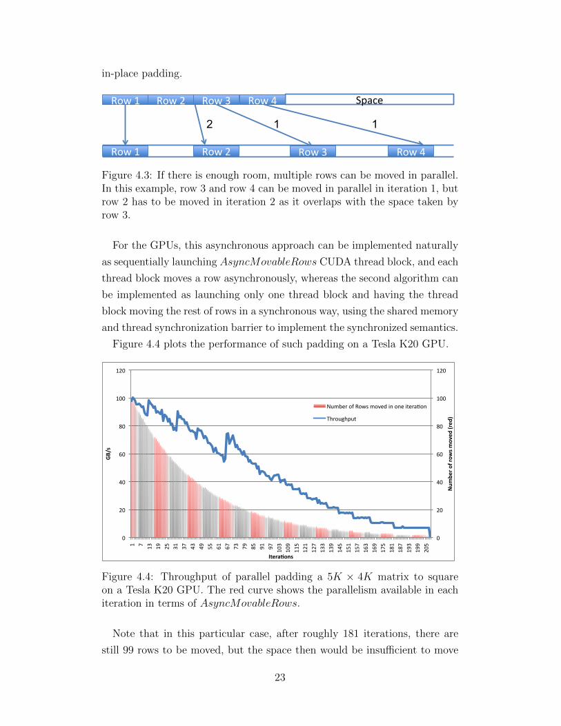
in-place padding.

Row  1   Space  

1 2

Row  2   Row  3   Row  4  

Row  1   Row  2   Row  3   Row  4  

1

Figure 4.3: If there is enough room, multiple rows can be moved in parallel.In this example, row 3 and row 4 can be moved in parallel in iteration 1, butrow 2 has to be moved in iteration 2 as it overlaps with the space taken byrow 3.

For the GPUs, this asynchronous approach can be implemented naturally

as sequentially launching AsyncMovableRows CUDA thread block, and each

thread block moves a row asynchronously, whereas the second algorithm can

be implemented as launching only one thread block and having the thread

block moving the rest of rows in a synchronous way, using the shared memory

and thread synchronization barrier to implement the synchronized semantics.

Figure 4.4 plots the performance of such padding on a Tesla K20 GPU.

0  

20  

40  

60  

80  

100  

120  

0  

20  

40  

60  

80  

100  

120  

1   7   13  

19  

25  

31  

37  

43  

49  

55  

61  

67  

73  

79  

85  

91  

97  

103  

109  

115  

121  

127  

133  

139  

145  

151  

157  

163  

169  

175  

181  

187  

193  

199  

205  

Num

ber  of  ro

ws  moved

 (red

)  

GB/s  

Itera6ons  

Number  of  Rows  moved  in  one  itera=on  

Throughput  

Figure 4.4: Throughput of parallel padding a 5K × 4K matrix to squareon a Tesla K20 GPU. The red curve shows the parallelism available in eachiteration in terms of AsyncMovableRows.

Note that in this particular case, after roughly 181 iterations, there are

still 99 rows to be moved, but the space then would be insufficient to move

23

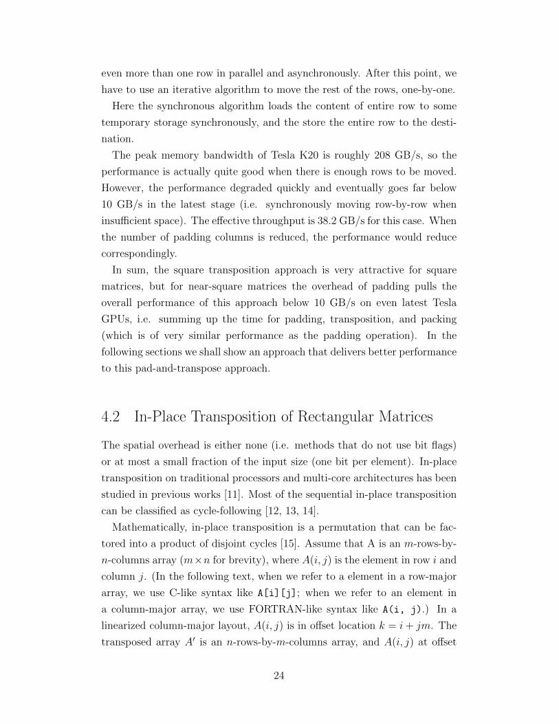
even more than one row in parallel and asynchronously. After this point, we

have to use an iterative algorithm to move the rest of the rows, one-by-one.

Here the synchronous algorithm loads the content of entire row to some

temporary storage synchronously, and the store the entire row to the desti-

nation.

The peak memory bandwidth of Tesla K20 is roughly 208 GB/s, so the

performance is actually quite good when there is enough rows to be moved.

However, the performance degraded quickly and eventually goes far below

10 GB/s in the latest stage (i.e. synchronously moving row-by-row when

insufficient space). The effective throughput is 38.2 GB/s for this case. When

the number of padding columns is reduced, the performance would reduce

correspondingly.

In sum, the square transposition approach is very attractive for square

matrices, but for near-square matrices the overhead of padding pulls the

overall performance of this approach below 10 GB/s on even latest Tesla

GPUs, i.e. summing up the time for padding, transposition, and packing

(which is of very similar performance as the padding operation). In the

following sections we shall show an approach that delivers better performance

to this pad-and-transpose approach.

4.2 In-Place Transposition of Rectangular Matrices

The spatial overhead is either none (i.e. methods that do not use bit flags)

or at most a small fraction of the input size (one bit per element). In-place

transposition on traditional processors and multi-core architectures has been

studied in previous works [11]. Most of the sequential in-place transposition

can be classified as cycle-following [12, 13, 14].

Mathematically, in-place transposition is a permutation that can be fac-

tored into a product of disjoint cycles [15]. Assume that A is an m-rows-by-

n-columns array (m×n for brevity), where A(i, j) is the element in row i and

column j. (In the following text, when we refer to a element in a row-major

array, we use C-like syntax like A[i][j]; when we refer to an element in

a column-major array, we use FORTRAN-like syntax like A(i, j).) In a

linearized column-major layout, A(i, j) is in offset location k = i+ jm. The

transposed array A′ is an n-rows-by-m-columns array, and A(i, j) at offset

24

k is moved to A′(j, i) at k′ = j + in after transposition. The equation for

mapping from k to k′ is:

k′ =

kn mod M, if 0 ≤ k < M

M, if k = M(4.2)

where M = mn−1. For transposing an m×n row-major array, the equation

is:

k′ =

km mod M, if 0 ≤ k < M

M, if k = M(4.3)

Since we are moving elements in-place, the destination an element is moved

to has to be saved and further shifted to the next location. Following this we

can generate a “chain” of shifting. For example, we can use a row-majored

5 × 3 matrix transposition example, i.e. m = 5, n = 3,M = mn − 1 = 14

as shown in Figure 4.5. We start with element 1, or the location of A[0][1]).

The content of element 1, or the location of A′[1][0]), should be moved to

the location of element 5, or the location of A[2][1]). The original content at

the location of element 5 is saved before being overwritten and moved to the

location of element 11, or the location of A′[2][1]); the original content at the

location of element 11 to the location of element 13, and so on. Eventually,

we will return to the original offset 1. This gives a cycle of (1 5 11 13 9 3

1). For brevity, we will omit the second occurrence of 1 and show the cycle

as (1 5 11 13 9 3). The reader should verify that there are five such cycles

in transposing a 5×3 row-majored matrix: (0) (1 5 11 13 9 3)(7)(2 10

8 12 4 6)(14).

An important observation is that an in-place transpose algorithm can per-

form the data movement for these five sets of offset locations independently.

This means that we only need to synchronize the data movement within each

cycle.

4.3 Parallelization of In-Place Transposition

As cycles by definition never overlap, it is an obvious source of parallelism

that could be exploited by parallel architectures. In fact, most of prior

25

0   1   2   3   4   5   6   7   8   9   10   11   12   14  13  

A

A’ (0,0) (1,0) (2,0) (3,0) (2,1) (0,1) (1,1) (4,0) (3,1) (0,2) (4,1) (2,2) (1,2) (3,2) (4,2)

(0,0) (1,0) (2,0) (0,1) (1,2) (2,1) (0,2) (1,1) (2,2) (1,3) (0,3) (0,4) (2,3) (1,4) (2,4)

Figure 4.5: Transposing a 5× 3 array A in the row-majored layout.

works [16] parallelize by assigning each cycle to a thread. However, for

massively parallel systems that requires thousands of concurrently active

threads to attain maximum parallelism, this form of parallelism alone is nei-

ther sufficient nor regular. Figure 4.6 shows the number of nontrivial cycles

in transposing the M × N matrix, 0 < M , N < 30 (i.e. |c| > 1 for a cycle

c). The diagonal case, where M = N , contains significantly more cycles than

the rest of the cases, but for the vast majority of other cases the amount of

parallelism from the sheer number of cycles is both much lower and varying.

Even for larger M and N , the parallelism coming from cycles can be low.

Also, as proven by Cate and Twigg [14], the length of the longest cycle is

always a multiple of lengths of other cycles. This creates significant load

imbalance problem for non-square matrices.

4.3.1 Locality Concerns of In-Place Transposition and TiledTransposition

It has been proven that the in-place transposition has poor locality as the

function of computing the next element is somewhat random [17]. This

problem can be alleviated at the expense of multiple memory accesses per

element as pointed out by multiple authors [18, 19, 10]. Essentially a full

transposition is decomposed to a series of tiled transpositions, as suggested by

Gustavson and others. This class of techniques tiles alleviate the poor locality

found in cycle following. Here we present a simplified version illustrating one

26

0 5 10 15 20 25M

0

5

10

15

20

25N

0

50

100

150

200

250

300

350

400

Num

ber o

f non

triv

ial c

ycle

s

Figure 4.6: Number of cycles available in transpositions up to 30× 30.

multi-stage transposition algorithm. For example, consider a 4× 2 matrix:0 1

2 3

4 5

6 7

To make it easier to see the memory locations, the matrix elements are

assigned values that are the same as their offset from the beginning of the

array. This can be treated as a 2× 2× 2 array (think of a two-by-one matrix

in which an element is actually a two-by-two matrix, like:[

0 1

2 3

][

4 5

6 7

]

So far we have not yet move any data, but merely view the data in a

different way. Now, a full transposition can be achieved by first conducting

27

two independent 2× 2 transpositions in-place, which leads to:[

0 2

1 3

][

4 6

5 7

]

If we again view the matrix from another perspective, this is equivalent to

a 2× 2 matrix in which each element is a 1× 2 vector:[(0, 2) (1, 3)

(4, 6) (5, 7)

]

We then transpose this matrix of 1× 2 vectors to:[(0, 2) (4, 6)

(1, 3) (5, 7)

]

And this matrix is indeed the transposed result:[0 2 4 6

1 3 5 7

]

Another way to see this sequence of transposition is to consider them

as dimension permutations. Suppose we label the three dimensions of this

logical (2 × 2) × 2 array as (M,N,O), respectively, the first transposition

effectively converts it to (M,O,N) (i.e. permutation 010! in the factorial

number system [20]), and the second transposition in turn converts the array

to (O,M,N) (permutation 100!). This notation is useful when there are more

dimensions in a permutation, which comes from tiling at not just rows but

also columns. Table 4.1 lists some of the permutations and their factorial

number. Intuitively, the factorial number for a particular permutation can

be thought as taking out an item from a imaginary queue of items, with

offset starting from zero for the leftmost element. If we insert items from

the right end of the queue and take the items from the left end of the queue,

we maintain the original order. However, when an item reaches the left end,

if we take its right neighbor instead for the next turn, we reverse the order

between the two items. If we have four items, (A,B,C,D) in the queue,

we can generate a sequence of four numbers by generating 0 whenever we

28

Table 4.1: Permutations in factorial numbering system.

#Dimensions From To Factorial Num.3D (A, B, C) (A, C, B) 010!

(A, B, C) (B, A, C) 100!

4D (A, B, C, D) (B, A, C, D) 1000!

(A, B, C, D) (A, C, B, D) 0100!

(A, B, C, D) (A, B, D, C) 0010!

remove the leftmost item (offset 0) and 1 for the item right to the leftmost

item (offset 1). So if we reverse the order between B and C, we would generate

0100!, which is the factorial number for a permutation from (A,B,C,D) to

(A,C,B,D).

So in the following text we shall use the factorial numbering system to

name the often-complicated dimension permutations. Note that by choosing

tile sizes carefully, the first transposition stage effectively permute individual

words in a much confined range in practical matrix sizes, thus improves

locality, and the second step effectively permutes large tiles over a much

wider address ranges, which is friendly to the memory hierarchy too as long

as the tile size is designed to convert at least a cache line (in the CPU context)

or coalesced memory access (in the GPU context).

4.4 Full Transposition as a Sequence of Elementary

Tiled Transpositions

We can generalize the simplified two-stage transposition we presented in the

previous section to support full transposition that tiles both row and columns.

According to Gustavson [16] and Karlsson [17] a full transposition of a matrix

can be achieved by a series of blocked transpositions in four stages.

The observation here is that the extra stages trade locality with extra

movements. On a modern NVIDIA K20 GPU, a four-stage Gustavson/Karlsson-

style in-place transposition reaches around 7 GB/s with optimized blocked

transposition whereas a single-stage in-place transposition only runs at 1.5

GB/s, due to poor locality.

To support general transposition of an M ×N matrix, we first consider it

as an M ′m by N ′n matrix where M = M ′m and N = N ′n. Assuming the

29

matrix is stored in row-major order, then one possible transposition sequence

of tiled transposition that Gustavson and Karlsson both mentioned is:

1. Treat matrix M ×N as a four-dimensional array of M ′ ×m×N ′ × n.

2. Perform M ′-instances of transposition that consists of super-elements

made of n elements, i.e. M ′ ×m×N ′ × n to M ′ ×N ′ ×m× n. This

is transposition 0100!.

3. Perform M ′ × N ′ instances of transposition, i.e. M ′ × N ′ ×m × n to

M ′ ×N ′ × n×m. This is transposition 0010!.

4. Perform a transposition of the M ′×N ′ matrix made of super-elements

of size n × m, i.e. M ′ × N ′ × n × m to N ′ ×M ′ × n × m. This is

transposition 1000!.

5. Perform M ′-instances of transposition that consists of super-elements

made of n elements, i.e. N ′ ×M ′ × n×m to N ′ × n×M ′ ×m. This

is also transposition 0100!.

An illustration of this approach can be found in Figure 4.7.

0 1 2 3

6 7 8 9

12 13 14 15

18 19 20 21

24 25 26 27

30 31 32 33

36 37 38 39

42 43 44 45

4 5

10 11

16 17

22 23

28 29

34 35

40 41

46 47

1. M x N = M' x m x N' x n

n=3N' = 2

m=2

M' =

4

M' x N' x m x n

m

N'

N'

m

0 1 2

3

6 7 8

9

12 13 14

15

18 19 20

21

24 25 26

27

30 31 32

33

36 37 38

39

42 43 44

45

4 5 10 11

16 17 22 23

28 29 34 35

40 41 46 47

0 1 2

3

6 7 8

9 4 510 110 1 2

6 7 8

0

1

2

6

7

8

12 13 14

15

18 19 20

21 16 1722 23

24 25 26

27

30 31 32

33 28 2934 35

36 37 38

39

42 43 44

45 40 4146 47

m

n

m

n

N'

M'

N'

M'

M' x N' x n x m

N' x M' x n x m0 1 2

3

6 7 8

9 4 510 11

12 13 14

15

18 19 20

21 16 1722 23

24 25 26

27

30 31 32

33 28 2934 35

36 37 38

39

42 43 44

45 40 4146 47

M'

n'

n'

M'

3 9

4

5

10

11

15 21

16

17

22

23

27 33

28

29

34

35

39 45

40

41

46

47

0

1

2

6

7

8

12

13

14

18

19

20

24

25

26

30

31

32

36

37

38

42

43

44

N' x n x M' x m

same as

same as

Transpose 100

Transpose 010

Transpose 1000

Transpose 100

2. Transpose 0100 is equal to M' transpose 100

3. Transpose 0010 is equal to M' transpose 010

4. Transpose 10005. Transpose 0100 is equal

to N' transpose 100

Figure 4.7: Four-stage full in-place transposition.

The reason for only using these three elementary transpositions is for local-

ity and parallelism: transpositions 1000! and 0100! move submatrices around,

whereas 0010! is effectively instances of individual permutations of elements

30

within submatrices. By carefully choosing the tile sizes and the stages taken,

fast on-chip memory can be utilized to hold tiles.

Although there seem to be three distinct tiled transposition involved (i.e.

0100!, 0010!, 1000!), they can all be derived from two basic ones. Transposi-

tion 0100! can be trivially implemented as M ′ parallel instances of transposi-

tion 100!, and transposition 1000! is just 100! with larger tiles. Transposition

0010 can be seen as 010! as well (treat the top two dimensions as one).

That is, transposition 0100! (e.g. ABCD to ACBD) can be treated as A

instances of transposition 100! on different tiles of BCD; transposition 0010!

(e.g. ABCD to ABDC) can be viewed as transposition 010! ((AB)CD to

(AB)DC). Transposition 1000! (ABCD to BACD) can be viewed as trans-

position 100! (e.g. AB(CD) to BA(CD)). So in the following sections we

shall describe parallelization strategies of these two elementary transpositions

for the GPU.

4.5 In-Place Transposition 010!

Effectively the transposition 010! performs many instances of transposition of

smaller tiles. Figure 4.8 illustrates one of such transposition of an M ′×m×Narray in row-majored layout.

One nice property of such tiled transposition is that it offers both locality

and parallelism: elements inside a tile are only permuted within the tile to

which they belong; transposition of different tiles are independent. Intuitively

transposing a tile can be assigned to a work-group (in OpenCL terms) or a

thread block (in CUDA terms) as for current GPU architectures, efficient

synchronization primitives like fast barrier as well as access to scratchpad

memory (local memory in OpenCL, or shared memory in CUDA).

If m×N is small enough to fit the register file, a very simple algorithm can

be used, assuming the variable temp is allocated to a thread-local register:

A straightforward extension to this approach can be done to use the

scaratchpad memory instead of the register file. In fact this approach works

fairly well (when it works): 95 GB/s can be achieved on an NVIDIA GTX480

GPU (with peak global memory throughput being 140GB/s).

For the cases where m×N is too large to fit the on-chip memory, we need

to look at the nature of this problem: this is the case where the capacity

31

M’ tiles

N

Fastest-Changing Direction

X X X X

X

X

Transpose a tile m

Figure 4.8: Transposition 010! as transposing many small tiles. At left itis equivalent to a 3D array [M′][m][N]; at right it is equivalent to [M′][N][m]after transposition 010!.

of temporary storage (be it the register file, or the scratchpad) is not large

enough to cover all the cycles in the transposition. This hence inevitably

suggests some algorithms that work by tracking only a subset of the cycles in

the transposition, holding the subset at some temporary storage, and shifting

these subsets.

Since transposition of each tile is independent, it is sufficient to consider

the problem as using an OpenCL work-group to transpose a smaller two-

dimensional array (i.e. an m×N tile in our previous example). Consider an

example, say (m,N) = (2, 5). Then the cycles in this 2 × 5 transposition is

(0)(1 2 4 8 7 5)(3 6)(9), assuming a row-majored layout. It should be

obvious that we can perform the data movement for the four cycles indepen-

dently.

32

1 for work-group k < M/m

2 parallel for (j < m)

3 parallel for (i < N)

4 // temp is private to each thread

5 float temp = data[k*m*N + j*N + i];

6 barrier(); // synchronize threads in a work-group

7 data[k*m*N + i*m + j] = temp;

A simple parallelization strategy is to have each cycle assigned to an

OpenCL work-item (or equivalently CUDA thread) somehow, and having

the work-items in the same work-group shift the entire m×N tile, and there

would be M ′ work-groups executing independently. It is however not trivial

to find the head of each cycle in advance, so one solution that leverages the

massive parallelism on GPUs is to have each work-item assigned an element

and attempting to follow the cycle the element belongs to, without actually

moving elements; if there is an element of lower address, the work-item ter-

minates itself; otherwise, the element is considered the head of the cycle and

the work-item would then actually perform the shifting.

This is a straightforward GPU parallelization of the cycle-following algo-

rithm IPT [16]; we call this P-IPT. The pseudo-code of this parallel version

of IPT is listed as follows:

1 parallel for i = 1 to m*N-2

2 k = P(i)

3 while k > i

4 k = P(k)

5 if (k == i)

6 shift the cycle starting from A[k]

7 end if

Note that the function P (i) is P (i) = i ∗m/(mN − 1).

However, as we pointed out earlier, both the number of cycles and their

lengths vary widely across different problem sizes, and also there may or may

not be enough cycles for massively parallel architectures like GPUs to fully

utilize its parallelism.

The overall idea is simple: we shall also parallelize the data movement

in a single cycle by having multiple threads to (somewhat) collaboratively

move the tiles within a long cycle. Meanwhile, we also need to make sure the

33

activities across multiple threads are orchestrated so that no data would be

overwritten prematurely.

To coordinate the shifting between threads working on the same tile, we

employ atomic operations and an mN -bit auxiliary storage to mark the fin-

ished tiles. The auxiliary storage is usually small enough to fit the on-chip

memory to allow fast atomic operations available to current GPUs. The

outline of this approach (Parallel-Tile-Transpose-Within-and-Across-Cycles

(PTTWAC)) for each work-group is shown in the Algorithm 1.

Algorithm 1: Parallel-Tile-Transpose-Within-and-Across-Cycles(PTTWAC).

Input: A: an M ′ ×m×N arrayOutput: A: an M ′ ×N ×m arrayData: done : m×N -bit array initialized 0 private to each work-group.

A bit i is set if the values of element i have been computed(not necessarily stored).

Data: R1,R2: private registers to each work-item; local id: uniqueID of each work-item within the work-group; group id: uniqueID of the work-group

Launch: M ′ work-groups that execute asynchronously. Each groupconsists of T threadsi← local id

for i < m×N − 1 doif done[i] 6= 0 then

Continue; /* Shifted; */

next in cycle←− (i ∗m)%(m ∗N − 1)if next in cycle == i then

Continue; /* Fix-point */

R1 ←− A[group id][i/N ][i%N ]while true do

R2 ←− A[group id][next in cycle/N ][next in cycle%N ]if atomic set(done[next in cycles]) 6= 0 then

Break;

A[group id][next in cycle/N ][next in cycle%N ]←− R1

R1 ←− R2

next in cycle←− (next in cycle ∗M) mod (M ∗N ′ − 1)

i← i+ T

Note the atomic set()2 operation attempts to set the bit specified by

2On current GPUs there are no bit-level atomic operations; one needs to simulate suchoperations with word-level atomics and bit masking operations.

34

the first argument in global memory and return the original value of that

bit. Also, in the implementation, the addressing of array A can be opti-

mized through pointer arithmetic: A[group id][i/N ][i%N ] is equivalent to

dereferencing A+m×N + i per the pointer-array duality in C.

Let us take the earlier example on transposing a 2×5 array in row-majored

layout, and simulate this algorithm within a single work-group. Assuming

9 work-items are launched, and only 4 work-items can be scheduled due to

hardware resource limitations in the following scenario; also recall the cycles

are (0)(1 2 4 8 7 5)(3 6)(9):

1. Work-items 0, 1, 2, 3 are scheduled. Then work-item 0 terminates

without copying. Work-items 1, 2, 3 load element 1, 2, 3 into their

private R1, load elements 2, 4, 6 into their R2, atomically set done[2],

done[4], done[6], and then store their R1 to elements 2, 4, 6.

2. Work-item 4 is scheduled as work-item 0 quits, and found element 4 is

shifted already (done[4] is set). Work-item 4 also quits. Work-items 1,

2, 3 load elements 4, 8, 3, and work-item 1 finds its next element (4) is

already shifted, so it quits. Work-items 2 and 3 atomically set done[8]

and done[3] and store to their next-element-in-cycles 8 and 3.

3. Work-items 5 and 6 are scheduled for execution since two work-items

quit in the previous step, and work-item 6 terminates immediately as

element 6 was shifted at step 2. Work-item 7 is then scheduled. Work-

items 7 and 5 shift elements 7 and 5 to elements 5 and 1.

4. All elements are now shifted; the remaining work-items 2, 3, 5, 7 quit.

In this scheme, the parallelism in shifting elements of the same cycle is

exploited: at step 3, work-items 2, 5, 7 are working on the largest cycle in

parallel, greatly improving the throughput of shifting. The spatial overhead

is small as we only need one bit for each element: the done array only takes

mN -bits overhead of compared to the original array of mN words; and the

bit-array can usually be stored in the on-chip memory as we pointed out

earlier.

Qualitatively speaking, because of the randomness of positions of elements

in the same cycle, sequentially scheduled work-groups may work on far-apart

portions in the same cycle (like how work-groups 2, 5 and 7 in step 3 worked

35

on tiles 8, 5 and 7. Intuitively, the longer the cycles, the larger the number

of work-groups will likely be working on them; thus balancing the loads of

work-groups dynamically.

4.5.1 Performance Improvements for Transposition 010!

In the cycle-following algorithm (i.e. PTTWAC), each work-item works on

shifting scalar values inside a tile. In order to ensure load balancing and

coalesced global memory reads, adjacent work-items start to read adjacent

elements and then follow the corresponding cycle. Also, one 1-bit flag per

element per tile is stored in OpenCL local memory, so that work-items can

mark the elements they shift. When one work-item finds a previously set

flag, it aborts the cycle. Here the baseline would be packing the flag bits

in local memory 32-bit words using an intuitive layout. The local memory

word Flag word, where the flag bit for element Element position is stored,

is given by Equation (4.4). Element position stands for the one-dimensional

index of an element within a tile.

Flag word = Element position/32 (4.4)

Due to the lack of bit-wise atomic operations, the flag bits are read and set

by using an atomic logic OR function that operates on 32-bit words. This

need for atomic operations will cause many collisions among work-items, spe-

cially in the initial iterations as Figure 4.9 explains. Particularly burdening

are intra-warp atomic conflicts,3 as explained by Gomez-Luna et al. [21]. In

that work, the authors showed the latency is roughly increased by a factor

equal to the number of colliding threads, that is called position conflict de-

gree. In order to illustrate this, let us consider the implementation of the

atomic logic OR operator to local memory in the NVIDIA Fermi instruction

set [22]:

1 /*0210*/ LDSLK P0, R7, [R9]; //Load from local memory

2 /*0218*/ @P0 LOP.OR R10, R7, R14; //Logic operation OR

3 /*0220*/ @P0 STSUL [R9], R10; //Store into local memory

4 /*0228*/ @!P0 BRA 0x210; //Conditional branch

3Warps are SIMD units in NVIDIA devices. AMD counterparts are called wavefronts.

36

The first instruction reads local memory addresses (words containing the

flag bits) and locks the access to them, in order to guarantee atomicity.

The next instructions are predicated, so that only those threads that have

acquired the locks execute the operation OR and store the result. Finally,

the remaining threads take the branch and try again.

0 1 2 3

4 5 6 7

8 9 10 11

12 13 14 15

16 17 18 19

20 21 22 23

Width

Tile

24 25 26 27

28 29 30 31

Tile in AoS

0 1 2 3 4 5 6 7 8 9 10 11 12 13 14 15 16 17 18 19 20 21 22 23 24 25 26 27 28 29 30 31

30 1 2 4 5 6 7 8 9 10111213141516171819202122232425262728293031 32 flags bits in one local memory word

Layout of the tile in global memory

(1) Consecutive threads read consecutive elements

(2) Threads access atomically flag bits in the same word

Figure 4.9: Consecutive work-items read consecutive elements in the tile (1).Their corresponding flag bits are stored in the same local memory word (2).This will provoke a position conflict degree equal to the warp (or wavefront)size. For the sake of simplicity, only eight threads of the warp (or wavefront)are represented.

The position conflict degree can be diminished by simply spreading the

flag bits over more local memory words. In Equation (4.5), the spreading

factor stands for the reduction in the number of flag bits per local memory

word. Thus, the maximum spreading factor is 32, unless the local memory

available becomes a constraint.

Flag word = Element position/(32/Spreading factor) (4.5)

Figure 4.10 illustrates the spreading in local memory. As it can be ob-

served, there is no need to change the exact location of each flag bit in the

corresponding local memory word. This does not influence the performance

of atomic operations.

The effect of spreading can be seen in Figure 4.11. This shows how the

bandwidth increases with the spreading factor (blue squares), for four test

problems included in Sung et al. [23]. Moreover, it presents the percentage

of divergent branches (red circles), that has been obtained with the com-

pute profiler. As explained previously, position conflicts match to divergent

branches. The inverse effect of reducing the branch divergence on the band-

width is noteworthy.

37

30 1 2 4 5 6 7 8 9 101112131415 16171819202122232425262728293031

30 1 2 4 5 6 7 8 9 10111213141516171819202122232425262728293031

30 1 2 4 5 6 7 8 9 131415 30 1 2 4 5 6 7 8 9 101112131415 30 1 2 4 5 6 7 8 9 101112 1415161718192021222324 30 1 2 4 5 6 7 8 9 10 2425262728293031

Spreading_factor = 1

Spreading_factor = 2

Spreading_factor = 4

Figure 4.10: The number of flag bits per local memory word is divided bythe spreading factor. Thus, the maximum possible spreading factor is 32.

00%

10%

20%

30%

40%

50%

60%

70%

80%

0

2

4

6

8

10

12

1 8 4 32 2 16 1 8 4 32 2 16 1 8 4 32 2 16 1 8 4 32 2 16

16 32 64 16 32 64 16 32 64 16 32 64

40 62 59 39

Bandwidth (GB/s) Divergent branches

Spreading factor Tile size

Test problem (Width)

Ban

dwid

th (G

B/s

)

Tesla C2050

Per

cent

age

of d

iver

gent

br

anch

es

Figure 4.11: Effect of spreading on bandwidth and percentage of divergentbranches. Tests were carried out on a NVIDIA Tesla C2050 GPU. Abscis-sas represent the spreading factor for different tile sizes and test problems(different width).

For a tiled transposition of m × N , if m is a power-of-two, say 32 or 64,

there will be new conflicts that are even more frequent when spreading the

flags, as it is explained in Figure 4.12 (a) and (b). This new conflicts can

be categorized as bank conflicts and lock conflicts. As explained by Gomez-

Luna et al., bank conflicts are due to concurrent reads or writes to different

addresses in the same local memory bank. Lock conflicts are caused by the

limited number of locks that are available in the hardware mechanism. This

produces a similar effect than position conflicts.

Padding can be used to remove both types of conflicts. This optimization

technique consists of keeping some memory locations unused, in order to

shift the bank or lock accessed by concurrent threads. For instance, as the

38

NVIDIA Fermi architecture contains 32 local memory banks and 1024 locks,

padding one word for each 32 words will remove most bank and lock conflicts.

This is shown in Figure 4.12 (c).

0 1 2 3 4 5 6 7

0 0 0 0 0 0 0 0 Flag_word

0 16 32 48 64 80 96 112

0 0 1 1 2 2 3 3

0 256 512 768 1024128015361792

0 8 16 24 32 40 48 56

0 1 2 3 4 5 6 7

0 1 2 3 4 5 6 7

0 16 32 48 64 80 96 112

0 16 32 48 64 80 96 112

0 256 512 768 1024128015361792

0 256 512 768 1024 1280 1536 1792

0 1 2 3 4 5 6 7

0 1 2 3 4 5 6 7

0 16 32 48 64 80 96 112

0 16 33 49 66 82 99 115

0 256 512 768 1024128015361792

0 264 528 792 1056 1320 1584 1848

Element_positionIteration 1

Iteration 2

Iteration 3

Position conflict

Position conflict

Bank conflict:16 mod 32 = 48 mod 32

Bank conflict

Bank conflictLock conflict:

512 mod 1024 = 1536 mod 1024Bank conflict

(a) Spreading_factor = 1 (b) Spreading_factor = 32 (c) Spreading_factor = 32& Padding

Figure 4.12: Consecutive work-items access consecutive elements in iteration1. In the following iterations, the next elements in the cycle are computedwith Equation (4.2). In this example, Tile = 16 and Width = 215, as oneof the test problems in Sung et al. Representative conflicts are highlighted:position conflicts (white), bank conflicts (yellow), lock conflicts (green). Incase (a), the flag word is obtained through Equation (4.4). Many positionconflicts appear. In case (b), the flag words are obtained with Equation (4.5).Position conflicts are removed, but bank and lock conflicts appear. The 32banks and 1024 locks are considered, as shown by Gomez-Luna et al. forNVIDIA Fermi architecture. In case (c), the use of padding avoids the lockconflicts and most bank conflicts.

Figure 4.13 shows the effect of padding on the bandwidth (top) and the

number of bank conflicts (bottom), that are measured with the compute

profiler. Although the effective impact on the bandwidth is not as impressive

as on the number of bank conflicts, it is noticeable a perceptible improvement

across the different tests. In these tests, the use of padding increases the

bandwidth up to 10%.

An alternative to spreading can be remapping the flag bits, that is, chang-

ing the way they are stored in local memory words. This could be useful

in those cases where the local memory size is not enough to employ spread-

ing. If the number of local memory words needed for storing flag bits is

39

0

50000

100000

150000

200000

250000

1 8 4 32 2 16 1 8 4 32 2 16 1 8 4 32 2 16 1 8 4 32 2 16

16 32 64 16 32 64 16 32 64 16 32 64

40 62 59 39

Bank conflicts No Pad

Bank conflicts Pad

Ban

k co

nflic

ts

Spreading factor Tile size

Test problem (Width)

3 4 5 6 7 8 9

10 11 12

1 8 4 32 2 16 1 8 4 32 2 16 1 8 4 32 2 16 1 8 4 32 2 16

16 32 64 16 32 64 16 32 64 16 32 64

40 62 59 39

GB/s No Pad GB/s Pad

Spreading factor Tile size

Test problem (Width)

Ban

dwid

th (G

B/s

)

Transpose 010 on Tesla C2050

Figure 4.13: Effect of spreading and padding on bandwidth and number ofbank conflicts. Tests were carried out on a NVIDIA Tesla C2050 GPU. Ab-scissas represent the spreading factor for different tile sizes and test problems(different width).

40

Num words, the remapping can be given by Equation (4.6):

Flag word = Element position mod Num words (4.6)

This ensures fewer position conflicts in the first iteration, but randomizes

more in the next ones. Thus, there is no synergy while applying the technique

together with spreading.

4.6 Transposition 100!

Algorithm that works for transposition 010! can be modified for transposition

100!. Since we are shifting T-sized tiles, not isolated elements in this case, we

have reasonably good locality for T larger than the wavefront size by having a

number of work-items shifting data values in each tile in a coalesced manner.

This implies that work-items in a work-group would be collaborating to move

tiles.

Again, here a simple solution is to have each cycle assigned to a work-group

and having the work-group shift the tiles in its assigned cycle sequentially,

i.e. P-IPT. The load imbalance is significant in this case: Our baseline GPU

implementation of this simple approach sees drastic performance variance

from 0.44GB/s to 13.65GB/s on NVIDIA Fermi, on the same array with

different tile sizes (16 and 64 respectively), which changes the aspect ratio of

array in terms of tiles and thus the cycles for moving tiles.

We can also adapt the PTTWAC algorithm for this type of transposition:

to coordinate the shifting between tiles working on the same tile, we employ

atomic operations and an MN ′-bit auxiliary storage to mark the finished

tiles. The outline of this approach for each work-group is shown in the

Algorithm 2.

Note this algorithm is essentially the PTTWAC mentioned by Sung et

al. [23]. While it does work reasonable well comparing to the P-IPT, this

predefined execution configuration poses some limitations:

1. The maximum possible Tile is limited to the maximum number of

work-items per work-group. This might be a considerable constraint in

some AMD devices, where the largest work-group size is 256.

41

Algorithm 2: Parallel-Tile-Transpose-Within-and-Across-Cycles(PTTWAC) for Transposition 100!

Input: A: an M ×N ′ array of T-sized tilesOutput: A: an N ′ ×M array of T-sized tilesData: done : M ×N ′-bit array initialized 0 private to each

work-group. A bit i is set if the values of tile i have beencomputed (not necessarily stored).

Data: R1,R2: private registers to each work-item; local id: ID ofeach work-item within the work-group

Launch: MN ′ − 1 work-groups that execute asynchronouslyforeach work-group i of size T in MN ′ − 1 work-groups do

if done[i] 6= 0 thenreturn

next in cycle←− (i ∗M)%(M ∗N ′ − 1)if next in cycle == i then

return; //no need to shift

/* Cooperatively load a tile i of A */

R1 ←− A[i][local id]while true do

/* Cooperatively load a tile at next in cycle */

R2 ←− A[next in cycle][local id]if local id = 0 then

if atomic set(done[next in cycles]) 6= 0 thenTerminates all work-item of the work-group

A[next in cycle][local id]←− R1

R1 ←− R2

next in cycle←− (next in cycle ∗M) mod (M ∗N ′ − 1)

42

2. As explained in the previous section, for power-of-two tile sizes, like

16, 32 and 64, they might entail even smaller work-groups than a warp

(32 work-items) or a wavefront (64 work-items) in current architec-

tures. Consequently, the SIMD lanes as well as L2 cache lines would

be underutilized.

3. Similarly, if Tile is not a multiple of warp/wavefront size, there will be

warps/wavefronts with idle work-items.

4. The use of barriers is needed to synchronize the warps/wavefronts be-

longing the same work-group. The synchronization also reduces mem-

ory parallelism from requests issued across warps/wavefront as they

now need to wait for each other.

4.6.1 Improving Flexibility and Performance

The aforementioned limitations encourage us to propose a new implemen-

tation that overcomes them. The gist is to use one SIMD warp/wavefront

to move m elements, instead of one work-group in Sung’s implementation.

This proposal is inspired on the warp-centric approach presented by Hong

et al. [24]. This optimization saves costly barriers that reduce the memory

level parallelism.

In the baseline implementation, each element of a tile was temporally

stored in one register per work-item. Since m will be usually longer than

the warp/wavefront size in our approach, local memory tiling is required in

the pursuit of flexibility. Figure 4.14 illustrates this technique.

First, each warp/wavefront will need several iterations to store its m ele-

ments in local memory. Then, the warp/wavefront will move its m elements

to the new location in global memory.

Further performance improvement can be achieved for particular cases

where m is a divisor or a multiple of the warp/wavefront size. The use of

register tiling will be more profitable than local memory tiling, because of

the highest bandwidth to registers [25].

43

Tile 1

Temporal storage in local memory

SoA in global memory

W1

W2

Tile

Width

Tile 1

ASTA in global memory

Tile 0

W0

Tile 0(1)

(2)

Figure 4.14: Warps/wavefronts store temporally the tile elements in localmemory (1). Each warp/wavefront needs several iterations to store its melements in local memory. Some work-items in warp/wavefront may remainidle during the last iteration (W2). Afterward, the warp/wavefront movesits m elements to a new space in global memory (2).

4.7 Three-Stage Full In-Place Transposition

When applying the 4-stage algorithm directly on the GPUs using the

PTTWAC algorithms, the performance of PTTWAC version of transposition

100! (A × B × C to B × A × C) depends entirely on the tile size C, and so

having large A and B does not affect performance as long as C is large

enough without overflowing on-chip memory. However, the transposition

1000! in the four-stage approach moves super-elements of m×n elements, so

a good (m,n) pair that works for transposition 1000! implies smaller m and

n for transposition 0100!, leading to sub-optimal performance.

Alternatively, we can eliminate the intermediate transposition 1000! with-

out sacrificing locality. One such improved 3-stage approach is:

1. Treat matrix M ×N as a three-dimensional array of M ×N ′ × n.

2. Perform transposition of n-sized super-elements, i.e. M × N ′ × n to

N ′ ×M × n. This is transposition 100!.

3. Treat matrix N ′×M×n as a four-dimensional array of N ′×M ′×m×n.

4. Perform N ′ × M ′ instances of transposition of m × n matrices, i.e.

N ′ ×M ′ ×m.× n to N ′ ×M ′ × n×m. This is transposition 0010!.

5. Perform N ′ instances of transposition of m-sized super-elements, i.e.

N ′ ×M ′ × n×m to N ′ × n×M ′ ×m. This is transposition 0100!.

44

In this improved algorithm, there are only three steps, and much larger m

and n can be used in the second and the last step respectively for transposi-

tion 0100! without overflowing the on-chip memory. An example is shown in

Figure 4.15.

0 1 2 3

6 7 8 9

12 13 14 15

18 19 20 21

24 25 26 27

30 31 32 33

36 37 38 39

42 43 44 45

4 5

10 11

16 17

22 23

28 29

34 35

40 41

46 47

1. M x N = M x N' x n

n=3N' = 2

M =

8

N' x M' x n x m0 1 2

3

6 7 8

9 4 510 11

12 13 14

15

18 19 20

21 16 1722 23

24 25 26

27

30 31 32

33 28 2934 35

36 37 38

39

42 43 44

45 40 4146 47

M'

n'

n'

M'

3 9

4

5

10

11

15 21

16

17

22

23

27 33

28

29

34

35

39 45

40

41

46

47

0

1

2

6

7

8

12

13

14

18

19

20

24

25

26

30

31

32

36

37

38

42

43

44

N' x n x M' x m

Transpose 100

5. Transpose 0100 is equal to N' transpose 100

4. Transpose 0010 is equal to N' transpose 010

0 1 2

6 7 8

0

1

2

6

7

8

m

n

m

n

Transpose 010

N'

M

M

N'

2. Transpose 100

Transpose 100

same as

0 1 2

3

6 7 8

9

12 13 14

15

18 19 20

21

24 25 26

27

30 31 32

33

36 37 38

39

42 43 44

45

4 5 10 11

16 17 22 23

28 29 34 35

40 41 46 47

3. N' x M x n = N' x M' x m x n

M' =

4

m = 2

Figure 4.15: Example of our improved approach to full transposition. Inevery figure, memory addresses increase from left to right and from top tobottom. Black halos represent super-elements, that are shifted as a whole.

Thanks to the PTTWAC algorithm we employed to implement transpo-

sition 100! on GPUs, the alternative approach is actually faster: the per-

formance of the PTTWAC version of transposition 100! ( M × N ′ × n to

N ′×M × n) depends entirely on the tile size, and so having a large M does

not affect performance as long as n is sufficient large. This saves one inter-

mediate transposition step without sacrificing locality. As we shall show, the

performance improvement of this approach is significant.

45

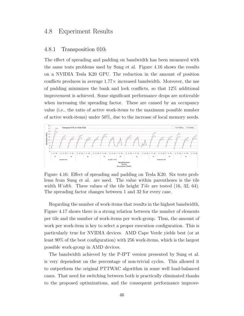
4.8 Experiment Results

4.8.1 Transposition 010!

The effect of spreading and padding on bandwidth has been measured with

the same tests problems used by Sung et al. Figure 4.16 shows the results

on a NVIDIA Tesla K20 GPU. The reduction in the amount of position

conflicts produces in average 1.77× increased bandwidth. Moreover, the use

of padding minimizes the bank and lock conflicts, so that 12% additional

improvement is achieved. Some significant performance drops are noticeable

when increasing the spreading factor. These are caused by an occupancy

value (i.e., the ratio of active work-items to the maximum possible number

of active work-items) under 50%, due to the increase of local memory needs.

5

7

9

11

13

15

17

19

21

23

1 4 16 2 8 32 1 4 16 2 8 32 1 4 16 2 8 32 1 4 16 2 8 32 1 4 16 2 8 32 1 4 16 2 8 32 1 4 16 2 8 32 1 4 16 2 8 32 1 4 16 2 8 32

16 64 32 16 64 32 16 64 32

bcsstk18 (40) bccstk31 (197) s3dkq4m2 (59)

w/o Padding w/ Padding

Spreading factor Tile size

Test problem (Width)

Ban

dwid

th (G

B/s

)

Transpose 010 on Tesla K20c

Figure 4.16: Effect of spreading and padding on Tesla K20. Six tests prob-lems from Sung et al. are used. The value within parentheses is the tilewidth Width. Three values of the tile height Tile are tested (16, 32, 64).The spreading factor changes between 1 and 32 for every case.

Regarding the number of work-items that results in the highest bandwidth,

Figure 4.17 shows there is a strong relation between the number of elements

per tile and the number of work-items per work-group. Thus, the amount of

work per work-item is key to select a proper execution configuration. This is

particularly true for NVIDIA devices. AMD Cape Verde yields best (or at

least 90% of the best configuration) with 256 work-items, which is the largest

possible work-group in AMD devices.

The bandwidth achieved by the P-IPT version presented by Sung et al.

is very dependent on the percentage of non-trivial cycles. This allowed it

to outperform the original PTTWAC algorithm in some well load-balanced

cases. That need for switching between both is practically eliminated thanks

to the proposed optimizations, and the consequent performance improve-

46

4 8

16 24

32

40% 50% 60% 70% 80% 90%

100%

16

52

88

124

160

196

232 40

76

112

148

184

220

256 28

64

100

136

172

208

244

16 32 64

4 8 16 24 32

Width Tile size

Nor

mal

ized

ba

ndw

idth

Transpose 010 on GeForce GTX 580

Warps /

Work

-grou

p

Figure 4.17: Choosing the execution configuration on NVIDIA GeForce GTX580. Tile is 16, 32 or 64, and Width changes between 16 and 256. Each seriescorresponds to a number of warps per work-group.

ment. Figure 4.18 shows the bandwidth for Width between 16 and 256 (Tile

equals 32) on GeForce GTX 580.

0%

20%

40%

60%

80%

100%

120%

140%

0

5

10

15

20

25

30

35

40

16

20

24

28

32

36

40

44

48

52

56

60

64

68

72

76

80

84

88

92

96

100

104

108

112

116

120

124

128

132

136

140

144

148

152

156

160

164

168

172

176

180

184

188

192

196

200

204

208

212

216

220

224

228

232

236

240

244

248

252

256

P-IPT PTTWAC-010-Base PTTWAC-010-Optimum Percentage

Width

Ban

dwid

th (G

B/s

)

Transpose 010 on GeForce GTX 580 Tile size = 32

Per

cent

age

of n

on-tr

ivia

l cyc

les

Figure 4.18: P-IPT version of transpose 010 compared to original PTTWACand optimized PTTWAC algorithm on GeForce GTX 580. Width changesbetween 16 and 256 and Tile is 32.

Finally, we have compared the optimized PTTWAC (with spreading and

padding) to the original algorithm for Width between 16 and 256 (in steps of

1) and Tile equal to 16, 32 and 64. The average speedup is 1.78 on NVIDIA

GeForce GTX 580, 1.84 on NVIDIA Tesla K20, and 1.79 on AMD Cape

Verde.

We have also tested the remapping of the flag bits. Although it improves

the original implementation, it is outperformed by the optimized version with

spreading and padding.

47

4.8.2 Transposition 100!

Figure 4.19 compares three PTTWAC implementations: the baseline that has

barriers, but without local memory tiling, one that uses local memory tiling

but eliminated the barriers, and one that assumes tile size being a multiple

of wavefront width with register tiling. Given test input N ×M ′ ×m of m

16, 32 and 64, and N between 16 and 256, the speedups are equal to 3.35

on GTX 580 and 3.05 on K20, when using local memory tiling. If register

tiling is applied, these speedups increase to 3.87 and 3.74, respectively. In

order to obtain the highest bandwidth, the work-group size has been chosen

to maximize the occupancy.

0

10

20

30

40

50

60

70

80

90

16

19

22

25

28

31

34

37

40

43

46

49

52

55

58

61

64

67

70

73

76

79

82

85

88

91

94

97

100

103

106

109

112

115

118

121

124

127

130

133

136

139

142

145

148

151

154

157

160

163

166

169

172

175

178

181

184

187

190

193

196

199

202

205

208

211

214

217

220

223

226

229

232

235

238

241

244

247

250

253

256

Original Local memory tiling Register tiling

Width

Ban

dwid

th (G

B/s

)

Transpose 100 on Tesla K20c Tile size = 64

Figure 4.19: Comparison of Sung’s original transpose to the new versions withlocal memory and register tiling. Tile is 64 and Width changes between 16and 256.

Unluckily, these speedups are not obtained on AMD Cape Verde, because

of the following facts:

• We have tested m equal to 16, 32 and 64. As the wavefront size is equal

to 64, there is no impact due to removing synchronization barriers.

• In NVIDIA devices the maximum number of work-groups per Streaming

Multiprocessor is limited (8 in Fermi) [26]. However, AMD devices

only limit the number of work-groups per Compute Unit (CU) to 16,

if the work-group is longer than a wavefront. Otherwise, the maximum

number of wavefronts per CU is 40 [27].

Anyway, the new versions add flexibility to the SoA-ASTA building block in

AMD devices as well.

Finally, the P-IPT version is always outperformed by the new versions on

NVIDIA devices. On AMD CapeVerde the local memory tiling version is

faster than the P-IPT version in most cases. It is slower for only 2% of the

tested cases, but at least 75% of the best P-IPT bandwidth is achieved.

48

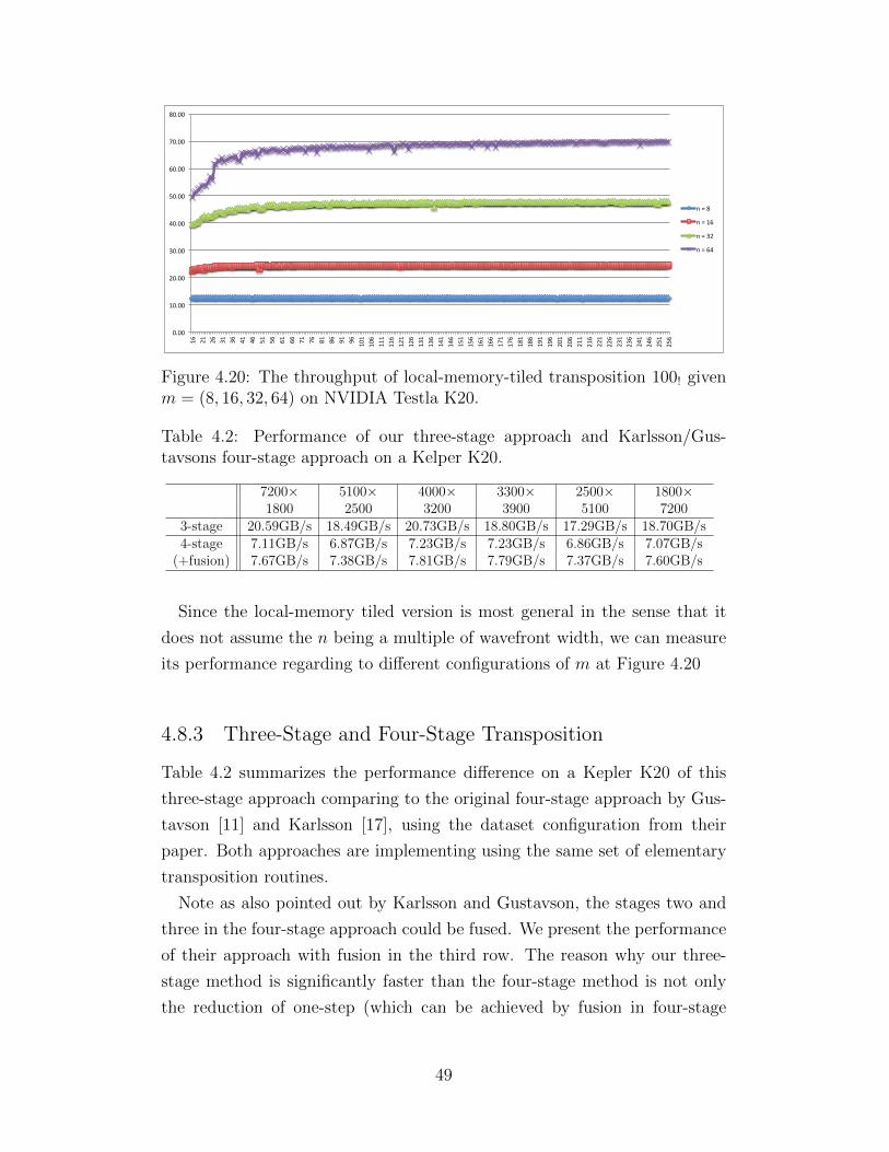
0.00  

10.00  

20.00  

30.00  

40.00  

50.00  

60.00  

70.00  

80.00  

16  

21  

26  

31  

36  

41  

46  

51  

56  

61  

66  

71  

76  

81  

86  

91  

96  

101  

106  

111  

116  

121  

126  

131  

136  

141  

146  

151  

156  

161  

166  

171  

176  

181  

186  

191  

196  

201  

206  

211  

216  

221  

226  

231  

236  

241  

246  

251  

256  

n  =  8  

n  =  16  

n  =  32  

n  =  64  

Figure 4.20: The throughput of local-memory-tiled transposition 100! givenm = (8, 16, 32, 64) on NVIDIA Testla K20.

Table 4.2: Performance of our three-stage approach and Karlsson/Gus-tavsons four-stage approach on a Kelper K20.

7200× 5100× 4000× 3300× 2500× 1800×1800 2500 3200 3900 5100 7200

3-stage 20.59GB/s 18.49GB/s 20.73GB/s 18.80GB/s 17.29GB/s 18.70GB/s4-stage 7.11GB/s 6.87GB/s 7.23GB/s 7.23GB/s 6.86GB/s 7.07GB/s

(+fusion) 7.67GB/s 7.38GB/s 7.81GB/s 7.79GB/s 7.37GB/s 7.60GB/s

Since the local-memory tiled version is most general in the sense that it

does not assume the n being a multiple of wavefront width, we can measure

its performance regarding to different configurations of m at Figure 4.20

4.8.3 Three-Stage and Four-Stage Transposition

Table 4.2 summarizes the performance difference on a Kepler K20 of this

three-stage approach comparing to the original four-stage approach by Gus-

tavson [11] and Karlsson [17], using the dataset configuration from their

paper. Both approaches are implementing using the same set of elementary

transposition routines.

Note as also pointed out by Karlsson and Gustavson, the stages two and

three in the four-stage approach could be fused. We present the performance

of their approach with fusion in the third row. The reason why our three-

stage method is significantly faster than the four-stage method is not only

the reduction of one-step (which can be achieved by fusion in four-stage

49

Table 4.3: Comparing our GPU implementation to Gustavson’s paralleltransposition for CPUs.

Processor Transposition Percentage ofthroughput sustained memory throughput

2x Intel Xeon L5420 (8 cores) 0.89GB/s [11] 18.2%2x AMD Operton 248 (8 cores) 0.36GB/s [11] 20.5%

NVIDIA K20 19.06GB/s 11.6%

approach anyway), but the three-stage algorithm allows much bigger tile

sizes which is crucial for transposition 100! and derived transpositions as we

have shown earlier. For Tesla K20, the performance of transposition 100!,

including derived 0100!, 1000!, is dominated by tile size used: 12.5 GB/s for

tile size 8, 24.5 GB/s for tile size 16, 47.6 GB/s for tile size 32, 69 GB/s

for tile size 64 on average. In fact, the best performing tile sizes (m,n) for

transposing a 7200× 1800 matrix is (20, 16) for four-stage transposition, but

(32, 72) for the three-stage algorithm on a Tesla K20.

If we compare that to the results reported by Gustavson [11] on multicores,

there is a drastic performance difference as shown in Table 4.3; the first

two rows shows results reported by Gustavson and the last row shows our

results. Although we have achieved a lower percentage of sustainable memory

throughput (measured by in-place load and store), comparing to Gustavson’s

design on multicores, we are able to achieve more than 20X speedup over their

implementation, thanks to the vast memory bandwidth available to GPUs.

Whereas we are achieving roughly 12% of the memory copy bandwidth on

a Tesla K20.

4.8.4 Choosing Tile Sizes for Full Transposition

Choosing the correct tile sizes is crucial to the performance of full transpo-

sition. Naıvely we could use some form of exhaustive search on all possible

m and n combination and use the best one, but that is too time-consuming

especially for M and N that have many possible dividends. We can prune

the search space by taking consideration of these three factors: Transposition

100! and 0100! work best if the tile size is larger. This limits the step two

(tile size = n) and step 5 (tile size = m) Transposition 0010! works best if

the tile (in this case m× n) fits into shared memory.

Figure 4.21 plots some of the best combinations of tile sizes (m and n) in

50

0  

50  

100  

150  

200  

250  

0   20   40   60   80   100   120   140   160   180   200  

n  

m  

90%+  of  20.59GB/s  

80%-­‐90%  

70%-­‐80%  

60%-­‐70%  

Figure 4.21: Tile sizes versus performance of transposing a 7200×1800 matrixin-place on a Tesla K20. Note the best-performing ones all fall in a very smallrange of tile sizes.

a 7200×1800 in-place transposition on one Tesla K20 Kepler. The best ones

achieved are 20.59 GB/s in an exhaustive search. It is clear that the tile sizes

that lead to best performance (80%+ of the best performing combinations)

are actually within a much small subset roughly along the curve of m× n <3600 (which is roughly the shared memory capacity) and with mostlym and n

around 60. Figure 4.22 plots the same but on an AMD Radeon HD7750 (Cape

Verde). We can see that, for AMD GPUs, the best performing combinations

are also confined in a small region, but the shape is different from an NVIDIA

GPU. For all three GPUs, a good guess for m and n will be from 50 to 100

with m × n less than the maximal shared memory capacity: this simple

heuristic can give you at least 80% of the best performance.

51

0  

50  

100  

150  

200  

250  

0   20   40   60   80   100   120   140   160   180   200  

n  

m  

90%+  of  8.75GB/s   90%-­‐80%  

80%-­‐70%   70%-­‐60%  

Figure 4.22: Similar trends can be seen on ATI GPUs. Note that the rangeof best-performing tile sizes are of different shape comparing to NVIDIA.

4.9 Related Work

4.9.1 In-Place Transposition

The research of transposition in-place has a long history. Berman [12] pro-

posed a bit-table for tagging cycles that has been shifted and it requires

O(mn) bits of workspace. Windley [13] presented the notation of cycle-

leaders as the lowest numbered element. Many works since then have con-

tributed the mathematical structure in in-place transposition. It is also worth

mentioning that Cate and Twigg [14] have proven a theorem to compute

the number of cycles in a transposition. Many works have been done in

the mathematical properties of in-place transposition. For improving cache

locality, many recent works took a four-stage approach [19, 17, 11]. For par-

allelization, Gustavson et al. [11] proposes parallelization for multicores up

to 8-cores. They also have noticed load imbalance issue even for the rela-

tively small number of threads available on multicores, comparing to modern

52

GPUs. For that problem, they proposed greedily assign each cycle to each

thread, and for long cycles they split the shifting a priori as described by

Gustavson [11].

4.9.2 In-Place and Out-of-Place Transposition for GPUs

For many-cores, previous work [9] has studied optimizations necessary for

high-performance out-of-place transposition. Sung et al. [23] proposed using

atomically-updated bit flags to solve the load-imbalance problem for the GPU

and proposes transposition routines that can be used to compose a multi-

stage transposition. However, their routines, especially transposition 100,

gives only less than 10% of the peak memory bandwidth available. They

also do not specify how one would apply these elementary transpositions to

obtain a full transposition.

4.9.3 Optimizing Atomic Operations on GPU

One widely used operation that is paradigmatic due to the intensive use of

atomic additions is histogram calculation. It has attracted research efforts

since the dawn of the GPU computing era [28, 29]. Recent works minimize

the impact of atomic conflicts by replicating the histogram in local memory

in combination with the use of padding [30] or a careful layout [31].

4.10 Summary and Future Work

We have presented the design and implementation of the first known full

in-place transposition of rectangular matrices for modern GPUs. We have

improved both the performance of building blocks proposed by earlier works

as well as the overall staged approach: combining with insights that lead

to greatly improved performance of elementary tiled transformations, a new

three-stage approach that is efficient for the GPUs is presented and we have

shown that this is much faster than traditional four-stage approaches. We

have also observed that the tile size greatly affects performance of in-place

transposition, especially for the GPUs since it can affect the algorithm choice

due to hardware limitations of on-chip resources. Though the search space

53

for tile sizes can be big, we have also identified pruning criteria that helps

the user to choose good tile sizes for current GPUs.

At a lower level, the elementary transpositions are improved by either re-

moving expensive barrier synchronization (for transposition 100!) or reducing

atomic contention (for transposition 010! algorithm that employs cycle follow-

ing). In the future we envision that a micro-architectural improvement to the

atomic operation hardware can be an viable approach to reduce contention

without padding, similar to earlier works that use exclusive-OR [32], skewed

addressing [33], and prime-number interleaving [34] to reduce contention in

either DRAM banks or set-associative caches.

54

CHAPTER 5

DATA LAYOUT TRANSFORMATION FORMEMORY COALESCING

1 Code reuse and data abstraction are commonly used in modern software

development practices. In an ideal world, these principles should be directly

applicable to the development of high-performance code for heterogeneous

computing as well. Unfortunately, there is an increasingly widening gap be-

tween what is considered good software development practice and what is

needed to generate high-performance kernels for heterogeneous platforms,

due to the underlying architecture differences between traditional CPU and

emerging massively parallel architectures. One of the major causes for this

gap is diverse data layout preferences of different parallel architectures. In

this chapter, we describe an attempt to mitigate the gap between what is

considered good code and what is considered fast code on current heteroge-

neous computing platforms, by designing and implementing a practical data

layout transformation system.

5.1 Motivation

5.1.1 Need for Reusable Kernels

The OpenCL standard promises portability of high performance heteroge-

neous parallel computing applications across a wide variety of CPU and

GPU hardware. While vendors such as AMD, Intel, IBM, and NVIDIA

have largely achieved functional portability of OpenCL applications to date,

there has been little reuse of OpenCL application kernels across hardware

platforms in practice. One problem that hinders the reuse of kernels is their

1This chapter includes parts of reprinted materials, with permission, from I.-J. Sung,G. Liu, and W.-M. Hwu, “DL: A data layout transformation system for heterogeneouscomputing,” in Innovative Parallel Computing (InPar), 2012, May 2012, pp. 1-11.

55

performance sensitivity to the diverse memory layout preferences of the un-

derlying hardware. Latency-optimized CPUs with a large amount of on-chip

cache memories use long cache lines and deep memory channel queues to

reshape transactions to the memory system and achieve high utilization of

the memory bandwidth. As long as the working set fits into the cache, the

achievable memory throughput is largely insensitive to the access patterns.

As a result, CPU data sets tend to assume layouts that follow the natural

organization used in external data files. For example, if each element of

an aggregate data set consists of several values, such as the RGB values of

a color pixel, the values for each data element are laid out in consecutive

memory locations, which is consistent with most natural file formats of video

cameras. Such a layout is commonly referred to as the array-of-structure

(AoS) layout.

Throughput-oriented many-core GPU systems tend to have much less on-

chip cache memory, if any, per parallel execution thread when compared to

their CPU counterparts. For example, the NVIDIA GTX480 GPU has a

relatively small cache capacity per thread (only 34 bytes of L2 cache mem-

ory per thread, given 1536 threads per SM, 15 SMs, and 768KB shared L2

cache). The main purpose of the last-level cache is to consolidate accesses

from parallel threads into fewer DRAM requests rather than to support tem-

poral reuse by capturing the working sets. Therefore, the achievable data

access bandwidth is much more sensitive to the access patterns of the mas-

sive number of simultaneously executing threads. As a result, NVIDIA GPUs

show strong benefit from data layout adjustments that minimize the number

of cache lines used by simultaneously executing threads. In the pixel exam-

ple, NVIDIA GPUs tend to prefer a data layout where all the R values of

the pixels processed by simultaneously executing threads are in consecutive

locations, followed by G values and then followed by B values. All these three

logical arrays (Rs, Gs and Bs) are parallel, meaning that arrays are accessed

simultaneously in an identical way according to the seminal C programming

language book [35]. Such layout is commonly referred to as the Structure-

of-Arrays (SoA) layout. In statically typed languages like OpenCL and its

base language C, the size of each (aggregate) field of a structure must be

known at compile time. This makes it extremely difficult, if not impossible,

to declare SoA types and pointers for dynamically allocated buffers where

the size of each field (array in this case) in the structure is unknown until

56

runtime. Unfortunately, the dynamically allocated buffers are the main use

mode of bulk data in OpenCL kernels. As a result, programmers tend to

break up the structure and simply use discrete, parallel arrays after they

transform the layout by hand. We will refer to this approach as the discrete

arrays (DA) layout.

5.1.2 Compound Data Objects and Heterogeneous Computing

“A set of parallel arrays suggest different organization of data,” as mentioned

in the classic C Programming book. Indeed, by creating a new type from a

collection of related data types one improves the readability of code. How-

ever, as described previously in Section 3.2, the layout of aggregate types

impose challenges to todays many-core GPU system. This is a more subtle

disparity of trends in the development of high-performance fine-grained par-

allel architectures and modern software engineering principles that is likely

to make the problem worse.

5.1.3 Memory Capacity

Due to the diverse layout preferences of CPUs and different types of GPUs,

neither AoS nor DA can satisfy the needs of all OpenCL hosts and devices.

Any data layout chosen by the programmer will likely perform poorly for

some parts of the application on some types of devices. This suggests some

form of conversion within the application. However, GPU DRAM capacity

is usually only a fraction of their CPU counterparts. Naive, out-of-place

data conversion can easily double the memory footprint. In some cases such

as large numeric applications, this can be a prohibitive factor. It is highly

desirable to perform marshaling in situ without requiring additional memory.

5.2 The Proposed Approach

We propose a holistic approach that intelligently maps and re-maps the data

structure used in application kernels into the most suitable layouts for un-

derlying GPU architectures in order to achieve good off-chip memory access

efficiency. We propose a new layout that (1) is friendly to vector access as

57

well as SIMT parallelism employed in current GPUs and (2) allows fast con-

version from and to array of structure types, and even the discrete arrays.

Second, we also propose fast, parallel marshaling algorithms that enables in-

place conversion of large AoS data structures within the constrained GPU

memory. Finally, a runtime system is employed to enable runtime marshal-

ing of OpenCL buffers at transformation boundary. To allow low-overhead

access to part of the converted data buffer in a multi-threaded environment,

the proposed runtime will also include on-demand, page-based dynamic mar-

shaling and coherence engine to ensure coherence of different logical layout

views of the same data structure.

The scope of this work is not limited to array-of-structures; converting from

dense array-of-structure to structure-of-array is not different from transpos-

ing a tall, dense matrix (assuming the number of elements per structure is

much smaller compared to the number of total structure instances). The

high-performance marshaling kernels developed by this work can hence be

applied to numerical problems that require fast in-place matrix transposi-

tion on the GPU. Also, this layout conversion system has been extended to

support sparse matrices that are laid out as rectangular arrays of (padded)

nonzero elements in each row.

5.3 Alternative Approaches

5.3.1 Compiler-Based Approaches

People have been trying to improve the memory locality within a structure by

splitting hot and cold structure members (and hot-and-cold objects) [36, 37].

These works aim to reduce the cache footprint when accessing large structures

in sequential programs by organizing frequently accessed elements within the

same structure instance. Assuming only a subset of members are accessed,

by reordering members the spatial locality can be improved. Our approach,

on the other hand, attempts to combine members across structure instances

from the same tile to improve both the vector access performance and locality.

58

5.3.2 Microarchitectural Approaches

Generally speaking, the proposed work helps reducing off-chip memory traffic

under strided access patterns. In this broad category, there are many related

works that take microarchitectural approaches. Some of them reduce the

impact on large strides that cause cache conflict misses and DRAM bank

conflicts [38], increases associativity [39], hides eviction cost [40]; some [41,

42] aim at improving SIMD performance through reducing on-chip memory

bank conflicts for small fixed strides.

5.4 Approach

The proposed approach consists of three parts: the ASTA layout which en-

ables a good tradeoff between performance and marshaling cost, and the

design of a dynamic runtime marshaling library for OpenCL.

5.4.1 The ASTA Layout

For array-of-structures that consists of structure elements of the same size,

one can actually consider the problem of converting AoS to SoA as trans-

posing the array. If we consider array-of-structures (AoS) as an M ′ × N

2-D array, then we can apply the full transposition algorithms we developed

earlier to obtain a structure-of-arrays (SoA) of N × M elements. As we

have shown earlier in Chapter 4, this conversion in general will need to take

up to three stages of intermediate transposition. However, there are two

observations that we can use to simplify the problem:

1. Unlike a general matrix, for array-of-structures it is common thatM >>

N , i.e. the number of elements inside a structure instance is usually

much smaller compared to the number of structure instances. For ex-

ample, a D3Q19 (i.e. three-dimensional, 19 quantities per element)

lattice-Boltzmann method code may have a structure size of 19, but

there will be millions of such structures. This means a very tall array

that allows us to just tile the M dimensions without worrying about

losing locality.

59

2. A CUDA warp/OpenCL wavefront consist of usually tens of SIMD

lanes, and so as long as the memory requests are of unit-stride from

threads/work-items within the same warp or wavefront has unit-stride,

they can be issued with a minimal number of memory requests.

These two observations lead to a simpler solution:

1. Treat an array-of-structures as an M ′ ×m×N array.

2. To obtain better SIMD memory access performance, use a layout that

is essentially M ′ ×N ×m.

We call the layout M ′ × N × m the Array-of-Structure-of-Tiled-Array

(ASTA) layout. By choosing m carefully we can apply the fast barrier-

synchronization version of transposition 010! to marshal the layout between

AoS and ASTA, and as long as m is large enough to cover the unit of memory

coalescing (half of warp size for current CUDA architectures), we should be

able to get reasonably good performance. In the following text, we shall call

m the tiling factor of an ASTA layout configuration.

Another way to see the ASTA layout is that we convert m adjacent struc-

ture instances into a mini SoA. In Listing 3.1, the structure type in Lines

15–18 and kernel ASTA shown in line 20 is an example of ASTA. Note the

struct foo 2 is derived from struct foo by merging four instances of struct

foo and generate a “mini SoA” out of each merged section. Effectively, each

scalar member in struct foo is expanded to a short vector in struct foo 2.

We call the length of this short vector (T ) the coarsening factor of the ASTA

type. The short vector is called a tile. Usually the coarsening factor is at

least the number of work-items participating in memory coalescing. ASTA

improves memory coalescing while keeping the field members of the same

original instance more closely stored, and is thus potentially useful to reduce

memory channel partition camping due to large strides [43, 9].

At a high level, marshaling from AoS to ASTA is similar to transposing M ′

instances of small T × S matrices. Whereas marshaling from DA to ASTA

is similar to transposing a matrix of S ×M ′ of T -sized tiles.

A similar technique can also be applied to sparse matrices that are stored

in a variant of the ELL [44, 45] format. This allows coalesced accesses along

the column direction in the example being vectorized in T-sized tiles. The

60

size of T is usually between 16 and 64 across GPU architectures for memory

coalescing. Note T is equivalent to the coarsening factor in ASTA.

5.4.2 Integrate the Layout Transformation and Marshaling

In the DL system, the need of specializing the marshaling kernels based

on structure type and coarsening factor is accommodated on-the-fly as an

integrated part of the kernel transformation process, and then invoked by

the marshaling runtime. This is described in the following sections.

While the data marshaling kernels described in this thesis could be and will

be exposed the OpenCL developers as a library of efficient layout-adjustment

routines, they can provide even more value as part of a transparent data lay-

out transformation system. In the DL system, the need of specializing the

marshaling kernels based on structure type and coarsening factor is accom-

modated on-the-fly as an integrated part of the kernel transformation process,

and then invoked by the DL runtime. As a result, the data marshaling ac-

tivities can be totally transparent to the host code. This is described in the

following sections.

5.5 Kernel Transformation and Runtime Marshaling

To automatically reconcile layout differences between the transformed kernels

at runtime, the system must be able to:

• Recognize the access pattern of the kernel.

• Transform accesses to buffers used by the kernel if necessary.

• Inform the runtime that the buffers need to be marshaled into desirable

layout before invoking the kernel.

At runtime, the runtime marshaling library must be able to:

• Marshal the kernel right before the kernel launch.

• Invoke the inverse marshaling kernel right before the transformed buffer

is copied back to host.

61

The system assumes that the dimensionality of the buffer is rectangular.

With this, it is possible to decouple the transformation and marshaling. Here

is a step-by-step description of the process using the AoS kernel in Listing 1.

Let us for now assume the kernel is transformed statically.

5.5.1 Step 1. Kernel Transformation

In this step the kernel is analyzed and transformed. We assume the user

exposes the dimensionality of buffers to the tool in the annotation in the

kernel source as shown in the following listing. The static transformation

tool parses the code and decides to transform it to ASTA, inserts a new

coarsened type and change the kernel code accordingly. The layout heuristic

is simple:

• Convert AoS to ASTA if detected on both architectures.

• Convert DA to ASTA for ATI architecture if the structure is larger

than a threshold of 10 floats (found by microbenchmarking).

To ease reading, the threshold is set to 1 float in the following example.

The transformed code is shown in the second half of the Listing 5.1. The

annotations are on lines 5 and 18; the code modified is on lines 7, 18 20 and

21.

After transformation, the tool inserts necessary information for the run-

time. In this case, the runtime needs the exact values that are available at

the moment the kernel is launched; i.e. the values of the dimensionality of

the transformed buffer, and the marshaling kernel to invoke. For the ex-

ample, the tool generated a marshaling kernel called AOS2ASTA foo into a

separate file that is accessible to the DL runtime and append its name to the

annotation so that at runtime, the marshaling kernel can be located.

62

1 struct foo{

2 float bar;

3 int baz;

4 };

5 //DL: AoS: f[global_size(0)]

6 __kernel void AoS( __global foo* f) {

7 f[get_global_id(0)].bar*=2.0;

8 }

9 struct foo{

10 float bar;

11 int baz;

12 };

13 struct foo_2{

14 float bar[4];

15 int baz[4];

16 };

17

18 //DL: AoS: f[global_size(0)] AOS2ASTA_foo

19 __kernel void AoS( __global foo* f) {

20 offset_t t1 = get_global_id(0);

21 f[t1/4].bar[t1%4]*=2.0;

22 }

Listing 5.1: Example of kernel transformation.

5.5.2 Step 2. Runtime Marshaling for OpenCL

An important feature of DL is to allow the host code to remain unchanged

when using a kernel with a transformed data layout. It also supports an

interface for incrementally transforming the host code components to use

transformed data layouts. This allows a development team to modify only

the performance-critical parts of an application to use the new data layout

and avoid the pitfall of requiring massive, wholesale changes to the entire

application. In fact, we envision that most of the host code will continue

to use the original data layout for many applications. DL achieves this by

63

supporting a dynamic marshaling mechanism that takes advantage of the

OpenCL memory model.

OpenCL requires explicit data transferring/remapping routines to transfer

data between host and device sides when invoking a kernel. Plus, OpenCL

memory buffers at the device side are explicitly created and managed through

a runtime library interface. The DL memory marshaling system has to keep

the semantics of the OpenCL memory model and transparently insert mar-

shaling calls only when necessary. Figure 5.1 shows a simple example of such

transparent marshaling.

The observation here is that we can infer the dimensionality and layout

of the OpenCL memory buffer if it is passed to a kernel that has special

marshaling requirement annotated in the source by static transformation.

Pass a cl_mem buf to a transformed kernel foo as arg0

Host DL Runtime

Record: 1.  foo(arg0buf) 2.  Need marshaling as foo

requires transformed arg0 Invoke kernel foo

1.  If out-of-place: •  Create a shadow

buffer buf’ •  Marshal from buf to

buf’ •  Call real OpenCL

kernel invocation with foo(arg0buf’)

2.  If in-place: •  buf and buf’ are the

same OpenCL buffer

Set arg0buf

Invoke foo(arg0buf’)

Marshal(bufbuf’)

free(buf)

Create new cl_mem buf’

Copy buf back to host memory

Set arg0buf’

1.  If out-of-place: •  Buf is already

transformed. Shadow buffer is buf’

•  Need marshaling as host requires original layout

•  Record buf’’ being the current shadow buffer of buf

•  If in-place: •  buf’ and buf’’ are the

same OpenCL buffer

Copy buf’’ back to host memory

Marshal(buf’buf’’)

free(buf’)

Create new cl_mem buf’’

Both in-place and out-of-place

Out-of-place only

Figure 5.1: An example of intercepting OpenCL runtime.

We use library interposition to hijack OpenCL library calls from the user.

For each transformed kernel K, each argument i is augmented with Ki ∈T × EN ×M derived from user annotation, where:

• T is the augmented types; T = Element Type ∪ {NIL}.

64

• E is a symbolic expression that defines the size of each dimension.

• M is the set of transformed and untransformed layouts; M = Γ∪{ξ}. ξmeans the layout is not transformed; Γ is the set of all layout transfor-

mations in this application. We represent a layout transformation as a

pair of handles to kernels generated by the runtime, one for converting

from the original to the transformed layout and one for converting back.

An example of such a pair is: (AOS2ASTA foo, AOS2ASTA foo inverse).

This specifies the requirement of that argument as well as the marshal-

ing kernels to invoke.

At runtime, each OpenCL memory buffer is augmented with a tuple S ×RN ×K, where:

• S specifies the current data layout of the buffer. S = {Uninitialized}∪ M.

• RN is the actual dimensionality of this buffer, where n is the number

of dimensions of this buffer from K.

• K is the last kernel argument this buffer has bound to.

At kernel launch time, the DL runtime evaluates each Ki to deduce actual

dimensionality and set the corresponding R. For the example this would be

[global size(0)]; the corresponding Ri is passed to the marshaling kernel so

that the buffer is correctly marshaled.

So, let us take the aforementioned example, and assume the kernel is

launched on 1024 work items. When the kernel K’s annotation is parsed by

DL runtime, the argument descriptor K0 of its only argument is: 〈T : foo,

n : 1, E : global size(0), M : AOS2ASTA foo〉. When a freshly initialized

OpenCL buffer is passed as f to the kernel, it is augmented dynamically by

DL runtime as: 〈S: ξ, R: the allocated buffer size, K: K0〉. When the ker-

nel actually launches, R is evaluated to be 1024 based on E=global size(0).

Then the DL runtime identifies a mismatch between S=ξ and T=AOS2ASTA foo

according to K0. So then the marshaling kernel corresponding to the trans-

formed layout (AOS2ASTA foo) is dynamically compiled and launched with

1024 work-items. After marshaling kernel completes, the buffer is augmented

as: 〈S : AOS2ASTA foo, R : 1024, K : K0〉. The kernel K is then launched

with the buffer in expected layout.

65

Should the buffer be later copied back to host code, then the inverse mar-

shaling kernel for layout AOS2ASTA foo is launched based on the descriptor

status right before the actual copying occurs, and the S would be reset to ξ.

If the buffer is used again by either the same kernel or another kernel with

the same T and evaluates to the same R, the marshaling is avoided. If there

is a mismatch between S and T and S 6= ξ, then we conservatively marshal

the buffer back to S = ξ then to T .

5.6 Results

The following OpenCL benchmarks are used:

• LBM, a computational fluid dynamics solver using the lattice-Boltzmann

method.

• SpMV, a sparse matrix-vector-multiplication kernel in ELL layout; each

row is stored consecutively.

• Black-Scholes, an option-pricing algorithm.

LBM and Black-Scholes are dense AoS layout codes whereas SpMV repre-

sents tall arrays constructed from sparse datasets. The first two benchmarks

are from the Parboil Benchmark Suite; the last benchmark is adapted from

NVIDIA OpenCL SDK.

For the SpMV benchmark, since the performance of layout conversion for

DA to ASTA could depend on the exact dimensionality of the dataset, we

use the following datasets listed Table 5.1.

Note that in ELL, the storage requirement for a matrix is the number of

rows times the maximum number of nonzero columns.

5.6.1 Application Results

Figure 5.2 and Figure 5.3 show the performance of the ASTA layout as well

as the generalization of tiled transposition on sparse matrix-vector multi-

plication (SpMV) on NVIDIA and ATI GPUs. For the LBM benchmark,

both the discrete array transformation and ASTA are able to boost the per-

formance by more than 4X (on NVIDIA) and roughly 3X (on ATI) if the

66

Table 5.1: Test problem for SpMV benchmark and DA-ASTA in-place mar-shaling.

Problem Description Size Max. #nonzerocolumns

bcsstk18 R.E. Ginna 11948× 40Nuclear Power Station 11948

e40r000 Driven cavity,40× 40 17281× 62elements, Re = 0 17281

bcsstk31 Stiffness matrix for 35588× 197automobile component 35588

bcsstk32 Stiffness matrix for 44609× 215automobile chassis 44609

s3dkq4m2 Finite element analysias 90449× 59of cylindrical shells 90449

conf6.0- Quantum 49152× 3900l8x8-8000 Chromodynamics 49152

marshaling cost is fully amortized. However, the ASTA layouts on both ATI

and NVIDIA architectures also outperform the DA layout. We believe that

the ASTA layout provides better locality and reduces potential bank con-

flicts that are more severe on ATI architectures, as current ATI GPUs have

simpler DRAM interleaving schemes [27]. Also, when dynamic marshaling

is employed, there is an additional marshaing cost for conversion of AoS to

DA. This will be addressed in the following sections.

For the SpMV benchmark, again both the tiled layout and fully transposed

layout can effectively improve the performance. On ATI architectures, the

tiled layouts in general are even faster than the full transpose kernel. We

also attribute this effect to shorter strides in the tiled transposition layout.

For blackscholes, moderate speedup is obtained on NVIDIA. On ATI, DA

is slightly faster than AoS and ASTA. That is because the structure size is

smaller compared to other applications: only five floats. And according to

our microbenchmark results earlier, for small structure sizes, AOS is even

faster. The reason why DA has speedup on ATI is that out of five elements,

two are used to store outputs. So DA may create a smaller cache footprint

as for outputs, other input elements need not to be brought into cache on

ATI architecture.

67

0  

2  

4  

6  

8  

10  

12  

LBM   BlackScholes   SpMV  (bcsstk18)  

AOS  

Discrete  Arrays  

ASTA(64)  

ASTA(32)  

ASTA(16)  

Figure 5.2: Application speedup on NVIDIA GTX480.

0  

0.5  

1  

1.5  

2  

2.5  

3  

3.5  

4  

4.5  

LBM   BlackScholes   SpMV  (bcsstk18)  

AOS  

Discrete  Arrays  

ASTA(64)  

ASTA(32)  

ASTA(16)  

Figure 5.3: Application speedup on ATI Radeon HD5870.

68

0  

1  

2  

3  

4  

5  

6  

1   2   3   4   5   6   7   8   9  10  11  12  13  14  15  16  17  18  19  20  21  22  23  24  25  26  27  28  29  30  

Speedu

p  over  AoS  

Itera.ons  

Discrete  Arrays  

ASTA(32)  

Figure 5.4: Net speedup including marshaling cost, LBM.

0  

0.2  

0.4  

0.6  

0.8  

1  

1.2  

1.4  

1.6  

1.8  

1   2   3   4   5   6   7   8   9  10  11  12  13  14  15  16  17  18  19  20  21  22  23  24  25  26  27  28  29  30  

Speedu

p  over  AoS  

Itera.ons  

Discrete  Arrays  

ASTA(32)  

Figure 5.5: Net speedup including marshaling cost, Black-Scholes.

69

0  

2  

4  

6  

8  

10  

12  

1   2   3   4   5   6   7   8   9  10  11  12  13  14  15  16  17  18  19  20  21  22  23  24  25  26  27  28  29  30  

Speedu

p  over  AoS  

Itera.ons  

Discrete  Arrays  

ASTA(32)  

Figure 5.6: Net speedup including marshaling cost, SpMV (bcsstk18).

Performance of Layouts with Marshaling Costs

To further understand the cost of layout conversion, or marshaling, Fig-

ures 5.4, 5.5 and 5.6 show the overall speedup including marshaling. Note

that the cost of marshaling is amortized as the number of iterations in-

creases. The blue curves of all subfigures (DA) are constantly below the red

ones (ASTA), showing that much more iterations are required to amortize

the cost of AoS to DA conversion, and in some cases the net speedup of

AoS to DA layout conversion is even below 1.0 given 30 iterations. Whereas

AoS to ASTA gives much better overall speedup and break-even point: at

most four iterations are required to break even with the marshaling cost.

Although DA and ASTA have generally comparable performance, clearly the

AoS to ASTA layout conversion is much faster than AoS to ASTA then to

DA conversion, especially if frequent dynamic layout conversion is required.

70

5.6.2 In-Place and Out-of-Place Marshaling

The ASTA layout, as well as the generalized tiled transposition for tall arrays

enable in-place marshaling on GPUs.

To evaluate its performance, we compare an implementation of a highly op-

timized out-of-place GPU matrix transposition method proposed by Ruetsch

and Micikevicius [9] with our in-place tiled transposition kernel.

Since the operation of marshaling does not involve any computation but

only memory loads followed by stores, it is sufficient to compare the memory

throughput of these two kernels. Table 5.2 shows the measurements using the

CUDA Compute Profiler on an NVIDIA GTX480 GPU on the e40r0000a

data set: a 17281 by 17281 sparse matrix stored in ELL format with at most

64 nonzero columns per row.

Table 5.2: Performance of full and tiled transposition kernels.

Marshaling Kernel Sustained Global Memory(ASTA tile size = 16) Bandwidth (in GB/s)AoS to SoA [9] 80.06(out-of-place)AoS to ASTA 82.23Barrier-sync (in-place)AoS to ASTA 19.64PTTWAC (in-place)

Both the out-of-place kernel and in-place barrier-sync-based kernel utilize

local memory to gain coalesced global memory accesses, which still seem to

be important for these memory-intensive kernels. On the other hand, cycle-

following transposition algorithms naturally suffer from load-imbalance and

poor locality. Our PTTWAC algorithm partly addresses the load-imbalance

by using atomic operations on parallelized shifts inside cycles, and the use

of ASTA layout confines the randomness of memory reference pattern in-

side a tile, which usually means a handful of cache lines. However, the

implementation still suffers from uncoalesced accesses as well as unneces-

sary contentions caused by simulating bitwise atomic operations on current

GPU architectures. Our PTTWAC-based AoS to ASTA implementation uses

atomic operations on local memory to reduce the cost, and uses atomic bit-

wise operations (AND and OR) to reduce the amount of memory requirement

for storing flags in local memory. These contributes to its lower performance.

In general, the AoS-to-ASTA PTTWAC algorithm should be consider as an

71

enabler on transposing larger ASTA tiles that are beyond the capability of

barrier-synchronization-based implementation, rather than a general solution

that can replace all other marshaling implementations.

The performance of SoA to ASTA marshaling naturally depends on the

number of cycles and cycle length, which are decided by the array size and

tile size. We thus compared the performance of two SoA to ASTA mar-

shaling approaches: parallelized IPT (P-IPT) and our algorithm PTTWAC

on converting various sparse matrices stored in transposed ELL format into

tiled transposed ELL format. These two can be considered as generalized

SoA and ASTA layouts.

4.75  

9.17  

15.10  

4.81  

10.02  

17.13  

4.63  

9.25  

17.11  

4.63  

9.30  

17.07  

4.62  

9.32  

17.12  

4.68  

9.56  

17.40  

0.44  

13.65  

0.85  

3.33  2.40  

27.35  

21.95  

25.06  

0.85  

0.00  

5.00  

10.00  

15.00  

20.00  

25.00  

30.00  

bcsstk18,  16  

bcsstk18,  32  

bcsstk18,  64  

e40r000a,  16  

e40r000a,  32  

e40r000a,  64  

bcsstk31,  16  

bcsstk31,  32  

bcsstk31,  64  

bcsstk32,  16  

bcsstk32,  32  

bcsstk32,  64  

s3dkq4m2,  16  

s3dkq4m2,  32  

s3dkq4m2,  64  

conf6.0,  16  

conf6.0,  32  

conf6.0,  64  

Sustaine

d  Mem

ory  Ba

ndwidth  (G

B/s)  

Sparse  Matrices,  Tile  Size  

PTTWAC  

P-­‐IPT  

Figure 5.7: Converting layouts from SoA to ASTA using PTTWAC andP-IPT.

The performance of P-IPT varies drastically over different input dimen-

sionality as well as ASTA tile sizes, as shown in Figure 5.7. Across all inputs,

PTTWAC performs smoothly and the only significant factor that affects its

performance is the tile size. For tile size 64, the performance varies from 15.0

GB/s to 17.40 GB/s, and then performance drops as tile size reduces. This

means the imbalance between cycle lengths does not manifest on PTTWAC.

However, the P-IPT algorithm, which only parallelizes across cycles, shows

unstable performance across inputs of the same tile sizes by almost 5x from

13.65 GB/s (bcsstk18, tile size 64) to 3.33 GB/s (e40r000a, tile size 64). This

matches our prediction that PTTWAC should able to dynamically balance

the load by allowing multiple work-groups works concurrently on long cycles.

Table 5.3 shows the performance of in-place AoS to ASTA transposition,

comparing both the approach that uses barrier synchronization (BS) and the

PTTWAC version. Note for larger tile sizes the BS approach does not work,

72

but when it works, the performance is very good.

Table 5.3: Performance of in-place AoS to ASTA transposition (GB/s).

PTTWAC BSProblem T=64 T=32 T=16 T=64 T=32 T=16bcsstk18 8.6 17.0 20.3 55.6 59.4 73.4e40r000a 6.9 14.0 19.6 51.2 61.0 82.2bcsstk31 5.3 5.8 8.2 NA 23.2 79.7bcsstk32 5.0 5.6 7.4 NA 23.8 80.6s3dkq4m2 7.1 16.6 21.3 61.3 67.0 93.1conf6.0- 11.7 19.2 20.6 67.9 67.9 86.8

5.7 Related Works

Jang et al. [46] proposed a methodology for changing the data layout to im-

prove memory coalescing. Zhang et al. [47] proposed a dynamic approach

to eliminate irregularities in GPU kernels. Che et al. [6] proposed a library-

based approach that performs marshaling on the CPU side and overlaps

PCI-e transfer with the CPU-side marshaling. All these approaches (includ-

ing ours) change the layout through redefining the mapping function that

flatten multidimensional indices into an offset for the layout. However, nat-

urally their marshaling performance is limited by the small CPU memory

bandwidth and they only allow marshaling between CPU and GPUs, not

among different GPU kernels. Also, their approach is equivalent of trans-

forming AoS to SoA, which only improves the memory coalescing but may

introduce partition camping as we observed.

In terms of tiling the data structure for memory parallelism, the method-

ology proposed by Sung et al. [43] is closely related to our approach. They,

however, only transform the kernel and expect manual changes on the host

side to reflect the changes in data layout.

On optimizing sparse matrix-vector multiplication, Choi et al. [48] pre-

sented manually optimized sparse matrix layouts to accelerate SpMV for

GPUs. However, only the construction, not the conversion between these

formats, is addressed.

73

5.8 Summary

We proposed the Array-of-Structure-of-Tiled-Array (ASTA) layout as a promis-

ing alternative to common discrete array transformation for improving the

global memory throughput for GPU applications that access data in Array-

of-Structure layout. ASTA not only provides better performance to discrete

arrays but also enables in-place marshaling on GPUs, which is crucial for

accelerators relying on high-throughput access to capacity-constrained pri-

vate DRAMs. We also show that ASTA allows much faster dynamic in-place

marshaling from AoS compared to discrete arrays, which implies a much

lower breakeven point in amortizing the marshaling cost compare to discrete

arrays.

We then generalize the ASTA to tiled transposed layouts for arrays that

have imbalanced aspect ratios, which is common for sparse matrices. We

show that for sparse-matrix transposition such a layout also provides com-

parable or even better performance for a fully transposed layout on sparse

matrix-vector kernels.

To allow developers to leverage the benefits of ASTA with minimal effort,

the proposed approach addresses the problem of decoupling host and device

layout needs through a user-friendly automatic transformation framework

that is designed and implemented in a transparent way to host code, even

allowing the user to keep host code unchanged while enjoying the benefit

provided by the system.

74

CHAPTER 6

DATA LAYOUT TRANSFORMATION FORMEMORY-LEVEL PARALLELISM

In this chapter, we discuss our second application of data layout transfor-

mation on modern many-core architectures such as the GPU: improving

memory-level parallelism through reducing channel and bank conflicts. An

important class of numeric application, or structured-grid code, is used in

this chapter as the driving examples.

As shown in Section 3.2, the sustained DRAM bandwidth to certain GPUs

can be greatly affected by strides in concurrent, in-flight memory accesses.

The root cause of this problem is that the design of modern GPUs is driven

by graphics workload, whose typical working-set size is too big to fit in any

reasonable cache system like CPUs, so the architecture of most GPUs does

not contain a large cache that is comparable to their CPU counterparts.

However, modern DRAM systems heavily rely on burst access, or a type

of request that accesses a continuous range of DRAM addresses. On typi-

cal CPU systems, usually the last level of cache line size maps directly to a

DRAM burst: when there is a cache miss, the cache controller would directly

ask a consecutive range of DRAM contents that corresponds to that cache

line. On GPUs, Bakhoda et al. reported that the property of locality of

many GPU workloads makes CPU-style caching unnecessary or even nega-

tively affecting performance [49]. Consequently, on modern GPUs the mem-

ory system is designed toward exploiting the spatial locality across memory

requests from SIMD lanes via memory vectorization (or memory coalescing),

and the parallelism across coalesced memory requests:

• Creating DRAM bursts by memory coalescing, or dynamically vec-

torizing scalar memory requests from a wavefront (OpenCL) or warp

(CUDA) into one or more wider DRAM bursts

• Using highly parallel interconnect that is capable of routing concurrent

memory requests to multiple DRAM channels.

75

Re#red  thread  blocks  

The  dynamic  set  of  simultaneously  ac#ve  thread  blocks   Unissued  thread  blocks  

Data  structures  in  GPU  global  memory  

Figure 6.1: Concurrently dispatched thread blocks (in CUDA) issuing mem-ory requests.

In current GPU programming models, users are allowed to launch a very

large number of work-groups (in OpenCL) or thread blocks (in CUDA), and

at runtime the blocks are issued somewhat sequentially to available processors

on the GPU, as shown in Figure 6.1. A processor can only execute a fixed

number of thread blocks as limited by resources like the number of registers

available. Once a thread terminates, a new thread block can then be issued

to the processor.

For data-parallel GPU kernels, the data is usually stored in the global

memory and then each thread works on a subset of data in a single-program-

multiple-data (SPMD) way. Typical programming practices generally involve

mapping thread IDs into data indices [50], so at a very high level, controlling

how thread indices are mapped into data offsets would change the locality.

Once memory requests are coalesced into bursts, as shown in Figure 6.2,

they are then routed to individual memory channels, as illustrated in Fig-

ure 6.3. As we stated earlier, the key to good performance is to make sure

these requests are somehow distributed well across the memory channels.

So far we have been addressing non-unit strides across nearby threads that

leads to poorly coalesced memory accesses. However, as we can intuitively

see from the second bullet point above, if the memory requests are not well

distributed across DRAM channels and banks, the memory throughput may

still degraded to just a fraction of the peak memory throughput. This is

also known as partition camping [26, 9], and is usually caused by having

very large strides (at the scale of multiple megabytes) across concurrently

76

Re#red  thread  blocks  

The  dynamic  set  of  simultaneously  ac#ve  thread  blocks   Unissued  thread  blocks  

Data  structures  in  GPU  global  memory  

Time

Memory coalescing

Figure 6.2: Coalesced memory accesses from threads in the same SIMD warp.

Re#red  thread  blocks  

The  dynamic  set  of  simultaneously  ac#ve  thread  blocks   Unissued  thread  blocks  

Time

Coalesced memory transactions

Memory  Interleaving  Hardware  

DRAM  Channels  

DRAM  Channels  

DRAM  Channels  

Figure 6.3: Coalesced memory accesses routed to different DRAM channels.

77

running threads.

One source of large strides is from accessing large multidimensional arrays

in a stencil-like manner. Many iterative solvers on structure grids have this

kind of access pattern and is hence interesting to apply data layout transfor-

mation to shorten the strides. For example, if we have a three-dimensional

array A of 500× 500× 500 32-bit floating-point numbers, and let us assume

that the array is laid out in row-major order, an expression like accessing

A[k][j][i]+A[k+1][j][i] would involve generating two memory references

that are 1000,000 bytes away from each other.

Structured grid applications [7] are a class of applications that calcu-

late grid cell values on a regular (structured in general) 2D, 3D or higher-

dimensional grid. Each output point is computed as a function of itself and

its nearest neighbors, potentially with patterns more general than a fixed

stencil. Examples of structured grid applications include fluid dynamics and

heat distribution that iteratively solve partial differential equations (PDEs)

on dense multidimensional arrays. When parallelizing such applications, the

most common approach is spatial partitioning of grid cell computations into

fixed-size portions, usually in the shape of planes or cuboids, and assign-

ing the resulting portions to parallel workers e.g. Pthreads, MPI ranks, or

OpenMP parallel for loops.

However, the underlying memory hierarchy may not interact in the most

efficient way with a given decomposition of the problem; due to the constantly

increasing disparity between DRAM and processor speeds [8], modern mas-

sively parallel systems employ wider DRAM bursts and a high degree of

memory interleaving to create sufficient off-chip memory bandwidth to sup-

ply operands to the numerous processing elements.

As we have pointed out in Chapter 2, unlike CPU-based systems in which

a DRAM burst usually corresponds to a cache line fill, massively parallel sys-

tems such as GPUs form a DRAM burst from vectorized memory accesses.

This can either be done by hardware from concurrent threads in the same

wavefront (also known as memory coalescing in CUDA terms) or by the pro-

grammer (such as the short-vector loads in CUDA and OpenCL). In both

cases, it is important to have concurrent accesses bearing desired memory

address bit patterns in terms of memory access vectorization. Intuitively

this can be addressed by loop transformations to achieve unit-strided access

in the inner loop. However, for arrays of structures, it is necessary to em-

78

ploy data layout transformations, such as dimension permutation, to achieve

vectorization [51] or reduce coherence overhead [52].

A less explored direction is the parallelism among memory controllers, and

interleaved DRAM banks, which plays an increasingly important role in sys-

tem performance. In massively parallel systems, the interconnection between

DRAM channels and processors decodes address bit fields to decide the cor-

responding channel and memory bank numbers from a memory request [49].

Given that a fixed subset of the address bits is used to spread accesses across

parallel memory channels and banks, achieving high bandwidth requires con-

currently serviced accesses to have varying values in those address bit fields.

To exploit this form of memory-level parallelism (MLP) in structured grid

applications, precise control must be exercised over how multidimensional in-

dex expressions map each index field to address bit fields. It is not generally

possible without data layout transformation or hardware approaches [53] to

shuffle address bit fields such that concurrent memory requests can be both

well-vectorized and routed to different memory channels and banks.

Unfortunately, the full details of the memory hierarchy are often too ob-

scure or complex for typical application programmers to adapt their programs

to these layouts. Even for the exceptional cases where the programmer does

know how to transform the data layout to fit the memory system, perform-

ing the transformation manually is tedious, results in less readable code, and

must be repeated every time a new platform is targeted.

6.1 Benchmarking and Modeling Memory System

Characteristics

For massively parallel architectures such as the GPU, the number of con-

current memory requests from all the processors can be large, especially for

codes with large datasets.

In such systems, the DRAM controllers spread these concurrent requests

through the interconnect into different memory channels and banks mostly

by hashing address bits. Moreover, on some systems such as the NVIDIA

G80 and GT200 GPUs, memory requests are vectorized (or coalesced, in

CUDA terms) based on the least significant bits of their addresses if these

requests are from a subset of threads that are executed in SIMD fashion (i.e.

79

CUDA warps) by the underlying hardware.

To better understand how memory interleaving works, it is necessary to

benchmark the underlying memory hierarchy to model the achieved memory

bandwidth as a function of the distribution of memory addresses of con-

current requests. As an example, we derive the analytical model for an

NVIDIA Tesla GPU, and use the execution model of that GPU to analyze

the expected program execution flow and the concurrent requests likely to

be generated. Other devices and programming models could be evaluated

independently with a similar approach. Previous work [25] benchmarked the

GPU to explore memory latency as a function of access strides in a single-

thread setting. However, since the class of applications we are targeting is

mostly bandwidth-limited, we must determine how the effective bandwidth

varies given access patterns across all concurrent requests. First, each mem-

ory controller will have some pattern of generating DRAM burst transactions

based on requests. The memory controller could be only capable of combining

requests from one core, or could potentially combine requests from different

cores into one transaction. In our example, the GPU memory controller im-

plements the former, with the CUDA programming manual [26] defining the

global memory coalescing rule, which specifies how transactions are gener-

ated as a function of the simultaneous requests from the vector lanes of one

streaming multiprocessor (SM).

Next, we must define our model on which bits in a memory address steer

interleaving among memory channels, DRAM banks, or other parallel distri-

bution structures built into the architecture to increase the number of concur-

rently satisfiable requests. We can determine these steering bits by observing

the behavior of a microbenchmark generating concurrent requests of a fixed

stride pattern and the resulting achieved bandwidth. The microbenchmark

is similar to pointer-chasing in lmbench [54]: each thread repeats the state-

ment x = A[x] for a large number of iterations, with the array A initialized

with A[i] = i and each thread initialized with x = blockIdx.x * Stride .

There is only one thread per thread block to ensure that each request results

in one memory transaction.

By examining the spikes of poor-performing bandwidth in Figure 6.4, we

can see a couple of features of the underlying system. First, each successive

power-of-two stride essentially generates a concurrent set of requests with a

fixed bit pattern in an increasingly large number of the lower address bits.

80

0

1

2

3

4

5

6

7

8

512

102

4

153

6

204

8

256

0

307

2

358

4

409

6

460

8

512

0

563

2

614

4

665

6

716

8

768

0

819

2

870

4

921

6

972

8

102

40

107

52

112

64

117

76

122

88

128

00

Milli

on D

RAM

Tra

nsac

tions

per

sec

ond

Stride (words)

Figure 6.4: Effective memory bandwidth vs. strides in words between re-quests from many single-threaded blocks on a NVIDIA Tesla GPU. Band-width is in millions of transactions per second, and strides are in incrementsof 64 words.

81

Continued performance degradation as the stride doubles indicates that the

bit that was variant in the previous power of two but not in the current

one is relevant to the parallel distribution of requests. Figure 6.4 shows

strides of 512, 1024, 2048, 4096 and 8192 words achieve successively lower

effective bandwidths. Although more detailed microbenchmarks suggest that

the interleaving is sophisticated enough that many of the higher bits may

contribute to steering to some degree, the most critical bits are those at

or below bit position 13. Second, the worst observed bandwidth occurs on

strides with a multiple of 512 words (2K bytes), indicating that the 11 lowest

bits have the most direct impact on achieved MLP. For instance, note that

strides of 8192+x*512 words are equally poor in performance as 8192 strides.

Through further detailed microbenchmarking, we have confirmed that all bit

positions in the range [13:6] are essential to spreading accesses to different

memory channels and banks. Therefore, for the purposes of data layout

of arrays of word-sized elements, we would consider the lower twelve bits

of a flattened index expression to be relevant (equivalent to address bits

[13:2]), and the bits in positions [10:6] the most important to vary across

burst requests and indeed sufficient to distribute accesses across all memory

system elements. From the coalescing rules [26], bits [5:2] are inferred to be

offsets into a DRAM burst. Within a burst, a good layout transformation

must maximize the number of useful words in that burst.

6.1.1 Common Access Patterns of PDE Solvers on StructuredGrids

Although there are many numerical methods that deal with PDEs, there are

only a few data access patterns among the most prevalent methods solving

these problems on structured grids. The structured grid often comes from

discretizing physical space with Finite Difference Methods [55] or Finite Vol-

ume Methods [56], while solutions based on Finite Element Methods [55]

often result in irregular meshes.

Many numerical methods solve PDEs through discretization and lineariza-

tion. The linearized PDE is then solved as a large, sparse linear system [57].

For large problems, direct-solution methods are often not viable: practical

approaches are almost exclusively iterative-convergence methods.

82

Iterative techniques like the Jacobi and Gauss-Seidel methods (including

those with successive overrelaxation) are often used as important building

blocks for more advanced solvers like multigrid [58]. Both techniques are

instances of stencil codes, whose stencils can be expressed as a weighted sum

of the cell and nearest neighbors in the grid. The major difference in terms

of access patterns is that Gauss-Seidel methods typically apply cell updates

in an alternating checkerboard style. Adjacent elements are never updated

at the same sweep; two separate, serialized sweeps over the red and black

cells perform one whole iteration update.

The lattice-Boltzmann method (LBM) [59], a particle-based method mainly

used in computational fluid dynamics problems, was recently extended as a

general PDE solver [60]. The LBM is also an iterative method applied to

structured grids. The cell update rules for the LBM are divided into two

stages that update multiple grid cell properties (i.e. distribution functions of

particles close to different edges or surfaces of the grid cell). The intra-cell

stage (called collide) and inter-cell stage (called stream) combined perform

one iteration’s update [61]. The stream stage accesses the nearest neighbors

of the current cell, while the collide stage’s inputs are entirely local to the

current cell. Since there is no data reuse within an update iteration across

cells, techniques that aim at reducing memory accesses such as shared mem-

ory tiling for the GPU are less useful. Hence, the LBM is considered memory

bandwidth-bound [62].

6.2 Data Layout Transformations for Structured Grid

C Code

For structured grid codes, transforming the bit patterns of effective addresses

of concurrent grid access expressions for the underlying memory hierarchy

can be achieved by transforming linearization functions calculating the grid

elements’ offsets from index expressions for each dimension and the size of

each dimension. This effectively transforms the data layout.

We first present a formalization of arrays, layouts, and layout transforma-

tions that define the required information as well as semantics. To conduct

data layout transformation, we collect the necessary information through

variable-length array syntax, a recently standardized feature of the C lan-

83

guage, that enables FORTRAN-style index expressions for arrays of all kinds,

including those whose size is not statically known. The extra information con-

tained in these declarations and accesses are essential to performing robust

data layout transformation.

6.2.1 Grids and Flattening Functions

Definition 1. An n-dimensional array G is characterized by an index space

that is a convex, rectangular subspace of Nn and type T.

An array element is identified by a vector of integers called an index vector.

Without loss of generality, for the index vector ~I of an array element, Ii ∈[0, Dimi) where Dimi ∈ N, Dimi > 0 is the i-th element of the dimension

vector of G. T is the type of all elements in G.

Definition 2. An injective function FF: Nn → N is a flattening function

for an n-dimensional array G if this function is defined for all valid array

element index vectors.

A flattening function defines a linearization of coordinates of elements in

G. When the resulting integer is interpreted as the offset for addressing an

element from the beginning of the memory space reserved for the array, then

this flattening function defines the memory layout of the array. We require

FF to be injective: it should map every valid index vector to a unique value.

An FF f explicitly forbids a many-to-one mapping, and thus f−1 is defined

and f−1(f(~I)) = ~I for a valid index vector ~I. With these restrictions, a

flattening function uniquely defines a memory layout and vice versa; we use

these terms interchangeably in the remaining text.

To permute the address bit pattern derived by an FF, we can transform the

Row-Major Layout (RML) flattening function by adapting the two following

primitive transformations proposed by Anderson et al. [63] that are analogous

to some well-known loop transformations:

Strip-mining: Split dimension i into T -sized tiles, 0 ≤ T < Di. This

transformation creates a new index vector ~I ′ and a new dimension

vector ~D′, which are inputs to the transformed FF. ~I ′ and ~D′ are created

by dividing Ii into Ih, Il and Di into Dh, Dl, where Ih = bIi/T c,Il = Ii mod T and Dh = dDi/T e, Dl = T . Intuitively, strip-mining

84

splits the dimension into two adjacent dimensions. When the original

dimension size is not a multiple of the strip size, padding is introduced

at the last strip.

Permutation: Permute the index vector and corresponding dimension vec-

tor.

Figure 6.5 shows a layout tiling example that transforms an access to array

A[Dj][Di] from A[j][i], i.e. RMLA, to A[jlog 2(Di):4][i][j3:0]. First the dimension

j is split into jH and jL without actually changing the order of elements in

memory, only padding the grid to some multiple of 24×Di elements. Then the

dimensions i and jL are swapped, which also changes the order of elements

in memory.

6.3 Directing Data Layout Transformation

Intuitively, the space of all possible layouts that can be derived by applying

the data layout transformation primitives arbitrarily on a multidimensional

data structure can be very large. However, by leveraging properties from both

the SPMD programming model, common on massively parallel systems, and

the class of applications we are targeting, we demonstrate a generalizable data

layout methodology for this application/target pair, based on an analytical

model of the memory hierarchy and static analysis of the program. Finally,

a data flow analysis is designed to help deduce data layouts for subscripted

pointer accesses in the program.

6.3.1 Data Transformation for Structured Grid Codes on aTwo-Level SPMD Programming Model

In current GPU architectures, each thread can only execute one memory

operation at a time. Concurrent requests are therefore generated from dif-

ferent threads executing concurrently on the parallel hardware. Intuitively,

index expressions dependent on thread and thread block identifiers should

have significant variations in their values, and therefore variations in the bits

representing the resulting address. To maximize bandwidth utilization, the

intuitive goal of data layout transformation is to ensure that the address bits

85

Figure 6.5: An example of layout transformation.

86

dependent on thread and thread block identifiers are the same as those bits

used in the memory system to distribute concurrent requests among paral-

lel memory system elements, and that the transformed access expressions

adhere to the coalescing rules for full utilization of DRAM bursts.

Let us first consider the CUDA-like pseudo code in Listing 6.1 that is a

simplified version of the 2D lattice-Boltzmann method (LBM).

1

2 enum {N=0, E, W, S};

3

4 // Declare A0 and Anext as 2D variable-

5 // length arrays of 4-element structures

6

7 __global__ void

8 example(int ny, int nx, float A0[ny][nx][4],

9 float Anext[ny][nx][4])

10 {

11

12 int i = threadIdx.x+1, j = blockIdx.x+1;

13

14 // Access in FORTRAN-like form

15

16 float x_velo = A0[j][i][E] - A0[j][i][W];

17 float y_velo = A0[j][i][N] - A0[j][i][S];

18

19 Anext[j][i-1][E] = x_velo;

20 Anext[j][i+1][W] = -x_velo;

21 Anext[j-1][i][N] = y_velo;

22 Anext[j+1][i][S] = -y_velo;

23 }

Listing 6.1: A running example.

In this code we have a 2D AoS layout. The code performs operations on

the input cell owned by the thread, using the results to update specific fields

of its neighbors in the output. Note that the leftmost dimension of every

index expression is some constant value plus blockIdx.x, the second dimen-

87

sion is always some constant plus threadIdx.x, and the last dimension is a

fixed offset denoting a structure field. The AoS layout is good for CPUs or

cache-based architectures in general because of better spatial locality among

structure members, but for GPUs this stops the memory vectorization hard-

ware (or memory coalescing hardware in CUDA terms) from fully utilizing

DRAM bursts when concurrent threads each requests a certain field of its

own cell. The coalescing rules effectively state that the index of the low-

est dimension must be dependent on threadIdx for good coalescing. This

issue can be easily resolved by permuting the data layout, perhaps by ex-

changing the second and last dimensions, leading to addresses that satisfy

the coalescing rule.

However, a good layout in terms of maximal MLP should also make con-

current memory accesses from different warps having distinct bits at those

steering bits. Intuitively, we should not only make a vectorizable access pat-

tern, but also assign bits of thread and thread block identifiers most likely to

be distinct among active threads to those steering bits. Identifying which

bits will be distinct among concurrent accesses requires analysis dependent

on the execution model of the architecture. A good data layout would take

these busy bits from the index of each dimension and map those bits into the

steering bits of the memory system. A more formal definition and automated

solution is presented in the remainder of this section.

6.3.2 Characterizing Thread Indices in Two-LevelSPMD Programming Models

In the two-level threading (thread/block) models employed by OpenCL and

CUDA, some properties regarding thread indices can be observed:

• Computational grids consist of fixed-sized thread blocks issued as a

whole to the processors (i.e. SM in CUDA terms). Distinct blocks are

executed asynchronously across processors. As for thread IDs, asyn-

chronous execution means that any thread with a legitimate thread ID

within a block can be the issuer of a memory request.

• The total number of blocks in the computational grid can be very large,

outnumbering the number of processors in the system, so the runtime

issues a subset of these blocks to the processors. In other words, at any

88

instant there is only a subset of X blocks being executed so the number

of distinct block ID usually is only a fraction of total number of blocks

in a computational grid. With some simplifying assumptions about the

regularity of block scheduling, the index range of currently executing

blocks can be roughly modeled as some oldest, still-executing block to

some youngest executing block with an index of X plus the index of

the oldest block minus one.

We can then characterize thread and block IDs in terms of distinct least

significant bits across their concurrent instances:

• The number of distinct least significant bits across concurrent block

IDs is about log2(maximum capacity of active blocks in the system).

• The number of distinct least significant bits across concurrent thread

IDs is about log2(block size).

For CUDA, the maximum capacity for active blocks in the system can be

determined statically from the compiled code’s resource usage and the device

parameters [26].

For our running example, assume there are 32 active thread blocks, each

with 128 constituent threads, which means 5 LSBs of a thread block index

and 7 LSBs of a thread index will be busy. In this case, one good layout

for array A0 could be created by strip-mining the Y and X dimensions by 32

and 128 respectively and shifting the resulting subdimensions into the steer-

ing and coalescing bit positions. In terms of dimension vector and flatten-

ing function, the dimension vector of A0 is ~D : (dny/25e, dnx/27e, 4, 25, 27) ,

where nx and ny are from C99 VLA declaration of A0; the FF of A0 is

FF (~I, ~D) : I2[:5]D3D2D1D0 + I1[:7]D2D1D0 + I0D1D0 + I2[4:0]D0 + I1[6:0],

where ~I is the index vector of the array subscripts, e.g. for A0[j][i][0],~I : (I2 = j, I1 = i, I0 = 0).

6.3.3 Automated Discovery of Ideal Data Layout

To automate the process of selecting and shifting bits to best fit the memory

system, we begin with a high-level algorithmic description of the procedure:

89

1. Convert all grid-accessing expressions into affine forms of thread and

thread block indices and surrounding sequential loop indices. For struc-

tured grid codes that use FORTRAN-like array subscripts, array ac-

cessing expressions can be usually converted to this form. In principle,

if there are non-affine terms in the expression, we could still approx-

imate it by introducing auxiliary affine terms, as suggested by Girbal

et al. [64].

2. For a given grid, if all the expressions accessing the grid share the same

coefficient for all columns except the constant column, then this grid is

eligible for layout transformation. We call the grid eligible, and define

a matrix consisting of coefficients of affine form of accessing expressions

except the constant column as the grid’s common access pattern. For

structured grid codes which access nearest neighbors, the access pattern

to the same grid usually has the same coefficient except for the last

column. For example, [x+1][y] and [x-1][y-1] are considered of the

same common access pattern

[1 0

0 1

](x

y

).

3. For each eligible grid, derive the desired data layout from its common

access pattern:

(a) Calculate the number of busy bits of each referred thread and

block index from the occupancy and thread block configuration.

(b) For each dimension, compute the collective busy bits represented

by the corresponding row in the common access pattern. Since a

row in the common access pattern represents some linear combi-

nation of thread and block indices, the collective busy bits are the

union of these busy bits, while some of them are possibly shifted

by log2 of their coefficients.

(c) Assign the least significant N bits of the fastest changing dimen-

sion index to the bit position that is used for memory coalescing,

where N is the number of address bits that determine memory

vectorization according to the hardware specification.

(d) Greedily assign other collective busy bits of all dimensions to the

steering bits by strip-mining power-of-two-sized tiles and permut-

90

ing these tiles to the desired bit position until steering bits are all

occupied or there are no busy bits left for any dimension.

(e) Assign all remaining bits to the higher dimensions.

(f) Generate flattening functions and dimension vectors according to

the above assignment and the C99 VLA declaration for the grid.

4. Perform dataflow analysis to derive the flattening function associated

with each array accessing expression.

5. Output the transformed code with inline-expanded flattening function

at grid accessing expressions.

For our running example, some of the access functions of A0 and Anext

are: (blockIdx.x + 1, threadIdx.x + 1, E), (blockIdx.x + 1, threadIdx.x +

1,W ), (blockIdx.x, threadIdx.x+ 1, N), and (blockIdx.x+ 2, threadIdx.x+

1, S). In the affine form of access functions similar to the notation used

by Girbal et al. [64], they would look like:

1 0 1

0 1 1

0 0 E

blockIdx.x

threadIdx.x

1

,

1 0 1

0 1 1

0 0 W

blockIdx.x

threadIdx.x

1

,

1 0 0

0 1 1

0 0 N

blockIdx.x

threadIdx.x

1

, and

1 0 2

0 1 1

0 0 S

blockIdx.x

threadIdx.x

1

, respectively. The affine form of the access func-

tions of Anext and A0 only differ in the last column, and thus both arrays

are eligible for data layout transformation, with their common access pattern

being

1 0

0 1

0 0

. The common access pattern clearly links the dimension with

individual thread and thread block indices, which are used for deciding the

actual layout based on their busy bits.

Continuing with our previous example, we will assume the number of active

thread blocks is 32, and the number of threads in the thread block is 128.

This means that the five least significant bits of blockIdx.x are busy, and

all seven meaningful bits of threadIdx.x are busy. The second dimension

index, corresponding to threadIdx.x, takes the lowest dimension place in

91

the transformed layout for coalescing (four least significant bits) and the

first three steering bits. The highest dimension is split into two dimensions,

with the five least significant bits accessing the new lower dimension and

the remaining bits accessing the higher dimension. The newly created lower

dimension is transposed to take the second lowest dimension of the new

layout. The remaining dimensions are left as they are, resulting in the layout

shown in Section 6.3.2.

6.3.4 Propagating Layout Information as Extended Typeswith Pointers

After each solver iteration, iterative PDE solver implementations in C or

C-like languages usually swap pointers to the input and output grid before

starting the next iteration, i.e. the output of the current iteration becomes

the input of the next iteration. Hence, correct propagation of layout and di-

mension information through pointer assignments is essential for these solver

implementations.

In other words, after deciding the layout of a specific grid, we need to

analyze the source code to figure out the set of grid access expressions, in the

form of subscripted pointer dereferences, that need to be updated to use the

transformed flattening function instead. We address this issue by treating

layouts as extended types and solve the dataflow equation to analyze the

layout for array accessing expressions.

Types in programming languages specify the information necessary for the

code to interpret and operate on instances of that type. The layout of an

array is an implicit part of an array’s type, typically defined by the language.

To transform the layout of a particular array, excluding other arrays, we

must essentially change that array’s type, and propagate that change in type

information through the program to ensure that all parts of the program

accessing that array do so correctly. This propagation could be performed at

runtime by extending the array type in the compiler to augment the grid with

a function pointer to the flattening function, set when the array is allocated.

However, current GPU programming models do not allow indirect calls, so

we elect to perform the propagation of the type change instigated by the

compiler in the compiler itself.

92

Table 6.1: Transfer functions.

Operation Type Transfer function f(µ) in the form of f(µ) = νwith ν(w) = µ(w)∀(w 6= p1) and ν(p1) = ...,where w ∈ P ;µ, ν ∈ Ψ

No definition involving any pointer vari-ables

ν(p1) = µ(p1) (identity function)

p1 = p2; p1 and p2 are pointers ν(p1) = µ(p2).

p1 = p2 + t; p1 and p2 are pointersand t is of integer type

ν(p1) = ⊥ if µ(p1) 6= UT else UT

Declaring a pointer p ν(p1) = UT

Declaring a pointer p to an n-dimensional grid G with a dimensionvector DV

ν(p1) = (n, DV,RML)

Apply layout transformation lt to thedata structured pointed by p1

ν(p1) = lt(µ(p1)) where lt is a layout transfor-mation.

Table 6.2: Meet function ∧.

l1 UT ⊥

l2 if l1 == l2

then l1 else ⊥⊥ ⊥

UT ⊥ UT ⊥⊥ ⊥ ⊥ ⊥

Therefore, we present algorithms for propagating the implicit layout type

information statically through a program, identifying the pointer references

that access the objects with extended types. The proposed usage scenario

is that the user specifies through annotation the grid on which the compiler

should perform automatic layout transformation, without specifying the ac-

tual layout, and the compiler decides the layout that works best on the given

grid for a given architecture, and propagates this layout information through

this analysis.

Our approach involves a source-to-source compiler that transforms the flat-

tening function of expressions accessing grids annotated with dimension vec-

tors, effectively deriving layout-transformed arrays, and finally emits CUDA

C code that can be further compiled by the NVCC compiler with inline-

93

expanded flattening functions on dynamically allocated one-dimensional ar-

rays.

We formulate this analysis as a monotonic dataflow analysis. In this frame-

work, a dataflow analysis is represented as a meet-semilattice and a set of

transfer functions. For this problem, the semilattice is (Ψ, ∧), where each

element in the semilattice is a function: Ψ : P → L ∪ {UT ,⊥}. P is the

set of pointer variables in the program, UT stands for untransformed and ⊥means incompatible respectively. L is a set containing the definitions of new

data layouts each fully defined by a dimension n ∈ N, a dimension vector Nn

and a flattening function Nn → N. When this function maps a pointer to a

new layout, it is asserting that every data structure the pointer may refer to

shares the specified layout. An untransformed pointer indicates that the data

structure it points to uses RML as its flattening function; an incompatible

pointer, however, indicates that this pointer may point to at least two data

structures with incompatible flattening functions. Two flattening functions

FF 1 and FF 2 are compatible (expressed as FF 1 == FF 2) if and only if for all

legitimate dimension vectors ~D and index vectors ~I, FF 1( ~D, ~I) = FF 2( ~D, ~I).

That is, the FF for a float array can be compatible with the RML for a long

array as long as their element sizes are the same. This allows transforming

the layout of some structured-grid code, in which non-float typed elements

are accessed through type-casted grid base pointer.

The set of transfer functions f : Ψ → Ψ are created from the type of

operations in the flow graph as shown in Table 6.1. The meet operation

of two functions m,n ∈ Ψ is defined in Table 6.2. In the table, the bi-

nary relationship == for two tuples {l1 = (n1, D1 ∈ Nexprn1 , FF1), l2 =

(n2, D2 ∈ Nexprn2 , FF2)} ∈ L exists if and only if n1 = n2 and D1 = D2 and

FF 1 == FF 2 . In a word, each statement, according to its operation type,

may change the layout bound to a pointer through assignment. Transformed

and untransformed layouts, as well as dimension vectors of grids, are thus

propagated.

The meet function ∧ deals with the join of control flow. Since most pro-

gramming models for the GPU do not allow indirect function calls in general,

for each grid access expression only one flattening function is allowed to bind

with that expression. The meet function basically aborts data layout trans-

formation for a particular grid if there are multiple incompatible flattening

functions that need to be bound with any expression that accesses the grid

94

(i.e. the binary relation == does not hold for these functions). This restric-

tion can surely be slightly relaxed using versioning, but this is left for future

work.

6.4 Experimental Results

Three CUDA benchmarks, namely CFD, Heat [65], and LBM [61], were used

to explore the significance of memory-level parallelism for memory-bound

structured grid applications and the validity of the data layout transforma-

tion heuristic presented in the thesis. CFD is an implementation of the

red-black Gauss-Seidel method for a 3D Navier-Stokes solver, Heat is a 3D

heat equation solver using the Jacobi method, and LBM is an implemen-

tation of the SPEC2006CPU [66] lattice-Boltzmann method. The first two

benchmarks represent the two major point methods for solving PDEs using

the finite difference method. LBM is an alternative CFD approach using a

particle-based method instead of discretizing the PDE. For each benchmark,

the performance of different layouts is presented in terms of the normalized

execution time over several ranges of grid sizes, changing the size of one di-

mension at a time. The experiments were run on a NVIDIA Tesla T10 GPU

with 4GB of memory.

We first manually convert each of the benchmarks into a layout-neutral

form and apply our automated layout transformation methodology on the

main grids on which it operates. Because our compiler infrastructure does not

yet support variable-length array syntax, we use annotations to communicate

that information to the compiler. After automatic transformation, the nearby

regions of the space of potential layout transformations where the solution

was found are manually searched for the best candidate.

The results show the criticality of a data layout for maximizing bandwidth

utilization by both vectorizing memory accesses into bursts, and parallelizing

them across interleaved memory channels and banks. The relative perfor-

mance of a layout depends on its divergence from the optimal layout in both

of these two criteria.

For the LBM benchmark, Figures 6.6-6.8 contrast the performance of the

layout derived from the transformation heuristic to the array-of-structures

(AoS) and structure-of-arrays (SoA) layouts. On average, switching from the

95

Figure 6.6: LBM, varying X.

Figure 6.7: LBM, varying Y.

96

Figure 6.8: LBM, varying Z.

AoS layout to the SoA layout improves the performance by 7.2X, mainly due

to improved burst-level parallelism from better memory coalescing. However,

the layout which maps busy bits to steering bits more prudently, thereby

achieving higher memory-level parallelism, further improves the performance

by 1.52X. Moreover, such a layout is more persistent to grid size variations.

Figures 6.9-6.11 show the merits of using an MLP-aware layout for the

Heat benchmark over a layout oblivious to it. While both layouts result in

fairly coalesced memory access patterns, the layout derived from the trans-

formation heuristic is 2.74X faster on average.

Figures 6.12-6.14 compare the performance of the layout of the CFD bench-

mark derived from the transformation heuristic to the default row-major

layout (RML) defined by the programming language. Effective tiling for the

memory interleaving hardware, which also results in marginally better mem-

ory coalescing, improves the performance of the derived layout by 1.16X on

average over RML.

Our experiments show that even with extra overhead computing memory

addresses, the transformed benchmarks still gain performance by improving

the efficiency of accessing memory. This highlights both the bandwidth-

boundedness of the benchmarks themselves, and the validity of trading extra

address calculation instructions for better bandwidth utilization in bandwidth-

97

Figure 6.9: Heat, varying X.

Figure 6.10: Heat, varying Y.

98

Figure 6.11: Heat, varying Z.

Figure 6.12: CFD, varying X.

99

Figure 6.13: CFD, varying Y.

Figure 6.14: CFD, varying Z.

100

bound applications.

6.5 Summary

We presented a formulation and language extension that enable automatic

data layout transformation for structured grid codes in CUDA. We also

benchmarked a NVIDIA Tesla GPU to reveal its DRAM banking and in-

terleaving scheme. Based on the microbenchmark results, we developed a

layout transformation methodology that can significantly speed up various

structured-grid codes by distributing concurrent memory requests evenly to

DRAM channels and banks.

Our methodology does not preclude opportunities of applying other trans-

formations that aims at improving reuse. Future work investigating holistic

data layout transformations addressing temporal locality, spatial locality, and

MLP will be paramount to achieving the highest levels of performance for

important, bandwidth-bound structured grid applications.

101

CHAPTER 7

CONCLUDING REMARKS

We have argued that:

• Efficient in-place transposition of rectangular matrices for the GPUs

can be done through composing elementary transpositions, in a novel

three-stage approach.

• Padding to square matrix and perform trivial in-place transposition

for square matrices is not a very attractive option on the GPU due to

limited parallelism.

• Array-of-structures can be considered as a tall matrix and we can use

fast tiled transposition to achieve good performance at a fraction of

cost comparing to a full transposition, which is effectively an array-of-

structure to structure-of-array conversion.

• Moreover, tiling multidimensional arrays found in structured-grid ap-

plications can improve memory level parallelism by creating hardware-

friendly strides for the underlying GPU memory interleaving system.

In the past decades, the trend of DRAM development requires increasingly

larger and larger burst lengths. This implies a widening gap on the memory

performance between truly random access and sequential access. For modern

massively parallel architectures like GPUs, it implies drastic performance

improvements if memory accesses are well vectorizable.

Many applications rely on transposition to gain such vectorizable access

as well as locality. We have presented the elementary transpositions that

exhibit good locality and balanced load thanks to efficient atomic operations

on the GPUs. We have also argued that a full transposition can be done in

three steps by composing these elementary transpositions.

The problem of matrix transposition can be generalized to handle the

array-of-structures that creates a working set that is too large for current

102

GPUs. We have demonstrated that full transposition which leads to a

structure-of-array layout is not necessary for good memory throughput. A

tiled layout that requires only one step of transposition can be used instead

and with very high conversion performance.

Finally, we have extended the methodology to increase not only the mem-

ory vectorization but also memory-level parallelism between vectorized mem-

ory requests by tiling the data structure in structured grid applications. This

lead to significant memory throughput improvements especially for GPUs

that does not have sophisticated memory interleaving schemes.

103

REFERENCES

[1] B. Keeth and R. J. Baker, DRAM Circuit Design: A Tutorial, 1st ed.Wiley-IEEE Press, 2000.

[2] M. Bian, F. Bi, and F. Liu, “Matrix transpose methods for SAR imagingsystem,” in Signal Processing (ICSP), 2010 IEEE 10th InternationalConference on, October 2010, pp. 2176 –2179.

[3] D. Bailey, “FFTs in external or hierarchical memory,” The Journalof Supercomputing, vol. 4, pp. 23–35, 1990. [Online]. Available:http://dx.doi.org/10.1007/BF00162341

[4] N. K. Govindaraju, B. Lloyd, Y. Dotsenko, B. Smith, and J. Manferdelli,“High performance discrete Fourier transforms on graphics processors,”in Proceedings of the 2008 ACM/IEEE Conference on Supercomputing,ser. SC ’08. Piscataway, NJ, USA: IEEE Press, 2008. [Online].Available: http://dl.acm.org/citation.cfm?id=1413370.1413373 pp.2:1–2:12.

[5] Y. Dotsenko, S. S. Baghsorkhi, B. Lloyd, and N. K. Govindaraju,“Auto-tuning of fast Fourier transform on graphics processors,” inProceedings of the 16th ACM Symposium on Principles and Practice ofParallel Programming, ser. PPoPP ’11. New York, NY, USA: ACM,2011. [Online]. Available: http://doi.acm.org/10.1145/1941553.1941589pp. 257–266.

[6] S. Che, J. W. Sheaffer, and K. Skadron, “Dymaxion: Optimizing mem-ory access patterns for heterogeneous systems,” in Proceedings of theACM/IEEE International Conference for High Performance Comput-ing, Networking, Storage and Analysis (SC), November 2011.

[7] K. Asanovic, R. Bodik, B. C. Catanzaro, J. J. Gebis, P. Husbands,K. Keutzer, D. A. Patterson, W. L. Plishker, J. Shalf, S. W. Williams,and K. A. Yelick, “The landscape of parallel computing research:A view from Berkeley,” EECS Department, University of California,Berkeley, Tech. Rep. UCB/EECS-2006-183, December 2006. [Online].Available: http://www.eecs.berkeley.edu/Pubs/TechRpts/2006/EECS-2006-183.html

104

[8] N. R. Mahapatra and B. Venkatrao, “The processor-memory bottleneck:Problems and solutions,” Crossroads, vol. 5, April 1999. [Online].Available: http://doi.acm.org/10.1145/357783.331677

[9] G. Ruetsch and P. Micikevicius, “Optimizing matrix transpose inCUDA,” NVIDIA Corporation, Tech. Rep., January 2009.

[10] M. Dow, “Transposing a matrix on a vector computer,” ParallelComputing, vol. 21, no. 12, pp. 1997 – 2005, 1995. [Online]. Available:http://www.sciencedirect.com/science/article/pii/016781919500050X

[11] F. Gustavson, L. Karlsson, and B. Kagstrom, “Parallel and cache-efficient in-place matrix storage format conversion,” ACM Transactionson Mathematical Software, vol. 38, no. 3, pp. 17:1–17:32, 2012. [Online].Available: http://doi.acm.org/10.1145/2168773.2168775

[12] M. F. Berman, “A method for transposing a matrix,” J. ACM,vol. 5, no. 4, pp. 383–384, Oct. 1958. [Online]. Available:http://doi.acm.org/10.1145/320941.320952

[13] P. F. Windley, “Transposing matrices in a digital computer,” TheComputer Journal, vol. 2, no. 1, pp. 47–48, 1959. [Online]. Available:http://comjnl.oxfordjournals.org/content/2/1/47.abstract

[14] E. G. Cate and D. W. Twigg, “Algorithm 513: Analysis of in-situtransposition [f1],” ACM Trans. Math. Softw., vol. 3, no. 1, pp. 104–110,1977. [Online]. Available: http://doi.acm.org/10.1145/355719.355729

[15] T. Hungerford, Abstract Algebra: An Introduction.Saunders College Publishing, 1997. [Online]. Available:http://books.google.com/books?id=H7XuAAAAMAAJ

[16] F. G. Gustavson and T. Swirszcz, “In-place transposition of rectangularmatrices,” in Proceedings of the 8th International Conference onApplied Parallel Computing: State of the Art in Scientific Computing,ser. PARA’06. Berlin, Heidelberg: Springer-Verlag, 2007. [Online].Available: http://dl.acm.org/citation.cfm?id=1775059.1775139 pp.560–569.

[17] L. Karlsson, “Blocked in-place transposition with application to storageformat conversion,” Umea University, Tech. Rep., 2009.

[18] W. Alltop, “A computer algorithm for transposing nonsquare matrices,”Computers, IEEE Transactions on, vol. C-24, no. 10, pp. 1038 – 1040,October 1975.

105

[19] S. D. Kaushik, C.-H. Huang, R. W. Johnson, P. Sadayappan, andJ. R. Johnson, “Efficient transposition algorithms for large matrices,”in Proceedings of the 1993 ACM/IEEE Conference on Supercomputing,ser. Supercomputing ’93. New York, NY, USA: ACM, 1993. [Online].Available: http://doi.acm.org/10.1145/169627.169814 pp. 656–665.

[20] D. E. Knuth, The Art of Computer Programming, Volume 3: Sortingand Searching. Redwood City, CA, USA: Addison Wesley LongmanPublishing Co., Inc., 1998.

[21] J. Gomez-Luna, J. M. Gonzalez-Linares, J. I. Benavides, and N. Guil,“Performance modeling of atomic additions on GPU scratchpad mem-ory,” IEEE Transactions on Parallel and Distributed Systems, vol. 99,no. PrePrints, p. 1, 2012.

[22] NVIDIA Corporation, cuobjdump. Application Note, January 2011.

[23] I.-J. Sung, G. Liu, and W.-M. Hwu, “DL: A data layout transformationsystem for heterogeneous computing,” in Innovative Parallel Computing(InPar), 2012, May 2012, pp. 1–11.

[24] S. Hong, S. K. Kim, T. Oguntebi, and K. Olukotun, “AcceleratingCUDA graph algorithms at maximum warp,” in Proceedings of the 16thACM Symposium on Principles and Practice of Parallel Programming,ser. PPoPP ’11. New York, NY, USA: ACM, 2011. [Online]. Available:http://doi.acm.org/10.1145/1941553.1941590 pp. 267–276.

[25] V. Volkov and J. W. Demmel, “Benchmarking GPUs to tune dense linearalgebra,” in Proceedings of the 2008 ACM/IEEE Conference on Super-computing, ser. SC ’08. Piscataway, NJ, USA: IEEE Press, 2008. [On-line]. Available: http://dl.acm.org/citation.cfm?id=1413370.1413402pp. 31:1–31:11.

[26] NVIDIA Corporation, CUDA C Programming Guide 5.0, July 2012.

[27] AMD, ATI Stream SDK OpenCL Programming Guide, Advanced MicroDevices (AMD), 2010.

[28] V. Podlozhnyuk, “Histogram calculation in CUDA,” NVIDIA Corpora-tion, Tech. Rep., 2007.

[29] R. Shams and R. A. Kennedy, “Efficient histogram algorithms forNVIDIA CUDA compatible devices,” in Proceedings of the Interna-tional Conference on Signal Processing and Communications Systems(ICSPCS), Gold Coast, Australia, December 2007, pp. 418–422.

106

[30] J. Gomez-Luna, J. M. Gonzalez-Linares, J. I. Benavides, andN. Guil, “An optimized approach to histogram computation on GPU,”Machine Vision and Applications, pp. 1–10, 2012. [Online]. Available:http://dx.doi.org/10.1007/s00138-012-0443-3

[31] G.-J. Braak, C. Nugteren, B. Mesman, and H. Corporaal, “GPU-vote:A framework for accelerating voting algorithms on GPU,” in Euro-Par 2012 Parallel Processing, ser. Lecture Notes in Computer Science.Springer Berlin Heidelberg, 2012, vol. 7484, pp. 945–956.

[32] Z. Zhang, Z. Zhu, and X. Zhang, “A permutation-based page interleav-ing scheme to reduce row-buffer conflicts and exploit data locality,” inProceedings of the 33rd Annual ACM/IEEE International Symposiumon Microarchitecture, ser. MICRO 33. New York, NY, USA: ACM,2000. [Online]. Available: http://doi.acm.org/10.1145/360128.360134pp. 32–41.

[33] B. Rau, “Pseudo-randomly interleaved memory,” in Computer Architec-ture, 1991. The 18th Annual International Symposium on, pp. 74–83.

[34] P. Budnik and D. J. Kuck, “The organization and use of parallel mem-ories,” Computers, IEEE Transactions on, vol. C-20, no. 12, pp. 1566–1569, Dec.

[35] B. W. Kernighan and D. M. Ritchie, The C Programming Language.Prentice-Hall, Inc., 1988.

[36] G. Chakrabarti, F. Chow, and L. PathScale, “Structure layoutoptimizations in the Open64 compiler: Design, implementation andmeasurements,” in Open64 Workshop at the International Symposiumon Code Generation and Optimization, 2008. [Online]. Available:http://www.capsl.udel.edu/conferences/open64/2008/Papers/111.pdf

[37] B. Calder, C. Krintz, S. John, and T. Austin, “Cache-conscious dataplacement,” in Proceedings of the Eighth International Conferenceon Architectural Support for Programming Languages and OperatingSystems, ser. ASPLOS-VIII. New York, NY, USA: ACM, 1998.[Online]. Available: http://doi.acm.org/10.1145/291069.291036 pp.139–149.

[38] Q. S. Gao, “The Chinese remainder theorem and the prime memory sys-tem,” SIGARCH Comput. Archit. News, vol. 21, no. 2, pp. 337–340, May1993. [Online]. Available: http://doi.acm.org/10.1145/173682.165172

107

[39] D. Sanchez and C. Kozyrakis, “The zcache: Decoupling ways andassociativity,” in Proceedings of the 2010 43rd Annual IEEE/ACMInternational Symposium on Microarchitecture, ser. MICRO ’43.Washington, DC, USA: IEEE Computer Society, 2010. [Online].Available: http://dx.doi.org/10.1109/MICRO.2010.20 pp. 187–198.

[40] J. Stuecheli, D. Kaseridis, D. Daly, H. Hunter, and L. John, “Coordinat-ing DRAM and last-level-cache policies with the virtual write queue,”Micro, IEEE, vol. 31, no. 1, pp. 90–98, Jan.-Feb. 2011.

[41] C. Gou, G. Kuzmanov, and G. N. Gaydadjiev, “Sams multi-layout memory: Providing multiple views of data to boost SIMDperformance,” in Proceedings of the 24th ACM International Conferenceon Supercomputing, ser. ICS ’10. New York, NY, USA: ACM, 2010.[Online]. Available: http://doi.acm.org/10.1145/1810085.1810111 pp.179–188.

[42] C. Gou and G. N. Gaydadjiev, “Elastic pipeline: AddressingGPU on-chip shared memory bank conflicts,” in Proceedings of the8th ACM International Conference on Computing Frontiers, ser.CF ’11. New York, NY, USA: ACM, 2011. [Online]. Available:http://doi.acm.org/10.1145/2016604.2016608 pp. 3:1–3:11.

[43] I.-J. Sung, J. A. Stratton, and W.-M. W. Hwu, “Data layouttransformation exploiting memory-level parallelism in structured gridmany-core applications,” in Proceedings of the 19th InternationalConference on Parallel Architectures and Compilation Techniques, ser.PACT ’10. New York, NY, USA: ACM, 2010. [Online]. Available:http://doi.acm.org/10.1145/1854273.1854336 pp. 513–522.

[44] “ITPACK 2.0 User’s Guide,” Center for Numerical Analysis, Universityof Texas, Tech. Rep. CNA-150, August 1979.

[45] N. Bell and M. Garland, “Efficient sparse matrix-vector multiplicationon CUDA,” NVIDIA Corporation, NVIDIA Technical Report NVR-2008-004, Dec. 2008.

[46] B. Jang, D. Schaa, P. Mistry, and D. Kaeli, “Exploiting memory ac-cess patterns to improve memory performance in data-parallel architec-tures,” Parallel and Distributed Systems, IEEE Transactions on, vol. 22,no. 1, pp. 105 –118, January 2011.

[47] E. Z. Zhang, Y. Jiang, Z. Guo, K. Tian, and X. Shen, “On-the-flyelimination of dynamic irregularities for GPU computing,” SIGARCHComput. Archit. News, vol. 39, pp. 369–380, March 2011. [Online].Available: http://doi.acm.org/10.1145/1961295.1950408

108

[48] J. W. Choi, A. Singh, and R. W. Vuduc, “Model-driven autotuningof sparse matrix-vector multiply on gpus,” in Proceedings of the 15thACM SIGPLAN Symposium on Principles and Practice of ParallelProgramming, ser. PPoPP ’10. New York, NY, USA: ACM, 2010.[Online]. Available: http://doi.acm.org/10.1145/1693453.1693471 pp.115–126.

[49] A. Bakhoda, G. L. Yuan, W. W. L. Fung, H. Wong, and T. M. Aamodt,“Analyzing CUDA workloads using a detailed GPU simulator,” in IEEEInternational Symposium on Performance Analysis of Systems and Soft-ware (ISPASS), 2009, pp. 163–174.

[50] D. B. Kirk and W.-M. W. Hwu, Programming Massively Parallel Proces-sors: A Hands-on Approach, 1st ed. San Francisco, CA, USA: MorganKaufmann Publishers Inc., 2010.

[51] B. Jang, P. Mistry, D. Schaa, R. Dominguez, and D. Kaeli, “Data trans-formations enabling loop vectorization on multithreaded data parallelarchitectures,” in PPoPP ’10: Proceedings of the 15th ACM SIGPLANSymposium on Principles and Practice of Parallel Programming. NewYork, NY, USA: ACM, 2010, pp. 353–354.

[52] Y.-L. Ju and H. G. Dietz, “Reduction of cache coherence overhead bycompiler data layout and loop transformation,” in Proceedings of theFourth International Workshop on Languages and Compilers for ParallelComputing. London, UK: Springer-Verlag, 1992, pp. 344–358.

[53] Y.-S. Kwon, B.-T. Koo, and N.-W. Eum, “Partial conflict-relieving pro-grammable address shuffler for parallel memories in multi-core proces-sor,” in ASP-DAC ’09: Proceedings of the 2009 Asia and South PacificDesign Automation Conference. Piscataway, NJ, USA: IEEE Press,2009, pp. 329–334.

[54] L. McVoy and C. Staelin, “lmbench: Portable tools for performanceanalysis,” in Proceedings of the 1996 USENIX Annual Technical Con-ference, 1996, pp. 23–23.

[55] K. W. Morton and D. F. Mayers, Numerical Solution of Partial Differ-ential Equations: An Introduction. New York, NY, USA: CambridgeUniversity Press, 2005.

[56] J. H. Ferziger and M. Peric, Computational Methods for Fluid Dynamics.Berlin: Springer, 1999.

[57] C. D. Gundolf, C. C. Douglas, G. Haase, J. Hu, M. Kowarschik, andC. Weiss, “Portable memory hierarchy techniques for PDE solvers, partII,” SIAM News, vol. 33, pp. 8–9, 2000.

109

[58] J. W. Demmel, Applied Numerical Linear Algebra. Philadelphia, PA,USA: Society for Industrial and Applied Mathematics, 1997.

[59] Y. H. Qian, D. D’Humieres, and P. Lallemand, “Lattice BGK modelsfor Navier-Stokes equation,” Europhysics Letters, vol. 17, no. 6, pp. 479–484, 1992.

[60] Y. Zhao, “Lattice Boltzmann based PDE solver on the GPU,” VisualComputing, vol. 24, no. 5, pp. 323–333, 2008.

[61] T. Pohl, M. Kowarschik, J. Wilke, K. Iglberger, and U. Rude, “Opti-mization and profiling of the cache performance of parallel lattice Boltz-mann codes,” Parallel Processing Letter, vol. 13, no. 4, pp. 549–560,2003.

[62] S. Ryoo, C. I. Rodrigues, S. S. Baghsorkhi, S. S. Stone, D. B. Kirk, andW.-M. W. Hwu, “Optimization principles and application performanceevaluation of a multithreaded GPU using CUDA,” in Proceedings ofthe 13th ACM SIGPLAN Symposium on Principles and Practice ofParallel Programming, ser. PPoPP ’08. New York, NY, USA: ACM,2008. [Online]. Available: http://doi.acm.org/10.1145/1345206.1345220pp. 73–82.

[63] J. M. Anderson, S. P. Amarasinghe, and M. S. Lam, “Data and com-putation transformations for multiprocessors,” SIGPLAN Not., vol. 30,no. 8, pp. 166–178, 1995.

[64] S. Girbal, N. Vasilache, C. Bastoul, A. Cohen, D. Parello, M. Sigler,and O. Temam, “Semi-automatic composition of loop transformationsfor deep parallelism and memory hierarchies,” Int. J. Parallel Program.,vol. 34, no. 3, pp. 261–317, 2006.

[65] K. Datta, M. Murphy, V. Volkov, S. Williams, J. Carter, L. Oliker,D. Patterson, J. Shalf, and K. Yelick, “Stencil computation optimizationand auto-tuning on state-of-the-art multicore architectures,” in SC08:Proceedings of the 2008 Conference on Supercomputing, Piscataway, NJ,USA, 2008, pp. 1–12.

[66] C. D. Spradling, “SPEC CPU2006 benchmark tools,” Computer Archi-tecture News, vol. 35, no. 1, pp. 130–134, 2007.

110