Cloud Futures 2011 Christopher Alme, Christopher Nunu Dennis Qian, Stanley Roberts Stephen Wong.

POLYNOMIAL CHAOS ANALYSIS OF MICRO AIR VEHICLES IN TURBULENCE
By
BRIAN CHRISTOPHER ROBERTS
A DISSERTATION PRESENTED TO THE GRADUATE SCHOOLOF THE UNIVERSITY OF FLORIDA IN PARTIAL FULFILLMENT
OF THE REQUIREMENTS FOR THE DEGREE OFDOCTOR OF PHILOSOPHY
UNIVERSITY OF FLORIDA
2012

c© 2012 Brian Christopher Roberts
2

I dedicate this to my parents.The best of me is a reflection of the love and support you have given.
3

ACKNOWLEDGMENTS
I would like to acknowledge the support I’ve received from the three mentors I have
had in Gainesville: Rick Lind, Mrinal Kumar, and Sheldon Cipriani. I have also received
support to make the wind tunnel work from my project possible from Simon Watkins
and Lawrence Ukeiley. Finally, I would like to acknowledge all of the students that I
have worked with over my five years in graduate school. Bouncing ideas off of each
other and engaging in sometimes heated discussions has given me the creativity and
understanding to complete a project of this magnitude.
4

TABLE OF CONTENTS
page
ACKNOWLEDGMENTS . . . . . . . . . . . . . . . . . . . . . . . . . . . . . . . . . . 4
LIST OF TABLES . . . . . . . . . . . . . . . . . . . . . . . . . . . . . . . . . . . . . . 8
LIST OF FIGURES . . . . . . . . . . . . . . . . . . . . . . . . . . . . . . . . . . . . . 9
ABSTRACT . . . . . . . . . . . . . . . . . . . . . . . . . . . . . . . . . . . . . . . . . 12
CHAPTER
1 INTRODUCTION . . . . . . . . . . . . . . . . . . . . . . . . . . . . . . . . . . . 13
1.1 Motivation . . . . . . . . . . . . . . . . . . . . . . . . . . . . . . . . . . . . 131.2 Problem Statement . . . . . . . . . . . . . . . . . . . . . . . . . . . . . . . 151.3 Research Plan . . . . . . . . . . . . . . . . . . . . . . . . . . . . . . . . . 16
1.3.1 Dissertation Outline . . . . . . . . . . . . . . . . . . . . . . . . . . 161.3.2 Contributions . . . . . . . . . . . . . . . . . . . . . . . . . . . . . . 171.3.3 Publication Plan . . . . . . . . . . . . . . . . . . . . . . . . . . . . . 18
2 TURBULENCE . . . . . . . . . . . . . . . . . . . . . . . . . . . . . . . . . . . . 19
2.1 The Nature of Turbulence . . . . . . . . . . . . . . . . . . . . . . . . . . . 192.2 Atmospheric Turbulence . . . . . . . . . . . . . . . . . . . . . . . . . . . . 232.3 Turbulence and its Impact on Aircraft . . . . . . . . . . . . . . . . . . . . . 242.4 Control in the Presence of Turbulence . . . . . . . . . . . . . . . . . . . . 26
3 FLIGHT DYNAMICS . . . . . . . . . . . . . . . . . . . . . . . . . . . . . . . . . 28
3.1 Aircraft Axis Systems . . . . . . . . . . . . . . . . . . . . . . . . . . . . . 283.1.1 Body-axis System . . . . . . . . . . . . . . . . . . . . . . . . . . . 283.1.2 Stability-axis System . . . . . . . . . . . . . . . . . . . . . . . . . . 283.1.3 Wind-axis System . . . . . . . . . . . . . . . . . . . . . . . . . . . 303.1.4 Earth-axis System . . . . . . . . . . . . . . . . . . . . . . . . . . . 30
3.2 Coordinate Transformations . . . . . . . . . . . . . . . . . . . . . . . . . . 303.2.1 Wind to Stability Frame . . . . . . . . . . . . . . . . . . . . . . . . . 313.2.2 Stability to Body Frame . . . . . . . . . . . . . . . . . . . . . . . . . 323.2.3 Earth to Body Frame . . . . . . . . . . . . . . . . . . . . . . . . . . 32
3.3 Nonlinear Equations of Motion . . . . . . . . . . . . . . . . . . . . . . . . 353.3.1 Dynamic Equations . . . . . . . . . . . . . . . . . . . . . . . . . . . 35
3.3.1.1 Force Equations . . . . . . . . . . . . . . . . . . . . . . . 363.3.1.2 Moment Equations . . . . . . . . . . . . . . . . . . . . . . 38
3.3.2 Kinematic Equations . . . . . . . . . . . . . . . . . . . . . . . . . . 403.3.2.1 Orientation Equations . . . . . . . . . . . . . . . . . . . . 403.3.2.2 Position Equations . . . . . . . . . . . . . . . . . . . . . . 42
3.3.3 The Equations Collected . . . . . . . . . . . . . . . . . . . . . . . . 43
5

3.4 Linearized Equations of Motion . . . . . . . . . . . . . . . . . . . . . . . . 44
4 WIND TUNNEL TESTING . . . . . . . . . . . . . . . . . . . . . . . . . . . . . . 49
4.1 Static Wind Tunnel Testing . . . . . . . . . . . . . . . . . . . . . . . . . . . 504.1.1 Wind Tunnel Setup . . . . . . . . . . . . . . . . . . . . . . . . . . . 504.1.2 Experimental Design . . . . . . . . . . . . . . . . . . . . . . . . . . 514.1.3 Results . . . . . . . . . . . . . . . . . . . . . . . . . . . . . . . . . 524.1.4 Analysis . . . . . . . . . . . . . . . . . . . . . . . . . . . . . . . . . 614.1.5 Conclusions . . . . . . . . . . . . . . . . . . . . . . . . . . . . . . . 65
4.2 Dynamic Wind Tunnel Testing . . . . . . . . . . . . . . . . . . . . . . . . . 654.2.1 Wind Tunnel Setup . . . . . . . . . . . . . . . . . . . . . . . . . . . 654.2.2 Experimental Design . . . . . . . . . . . . . . . . . . . . . . . . . . 684.2.3 Results . . . . . . . . . . . . . . . . . . . . . . . . . . . . . . . . . 69
4.2.3.1 Sweep Model . . . . . . . . . . . . . . . . . . . . . . . . . 704.2.3.2 Dihedral Model . . . . . . . . . . . . . . . . . . . . . . . . 72
5 POLYNOMIAL CHAOS THEORY . . . . . . . . . . . . . . . . . . . . . . . . . . 76
5.1 Background . . . . . . . . . . . . . . . . . . . . . . . . . . . . . . . . . . . 765.2 Theory . . . . . . . . . . . . . . . . . . . . . . . . . . . . . . . . . . . . . . 785.3 Linear System . . . . . . . . . . . . . . . . . . . . . . . . . . . . . . . . . 845.4 Difficulties . . . . . . . . . . . . . . . . . . . . . . . . . . . . . . . . . . . . 86
5.4.1 Numerical Issues . . . . . . . . . . . . . . . . . . . . . . . . . . . . 875.4.2 Modal Interpretation . . . . . . . . . . . . . . . . . . . . . . . . . . 88
5.4.2.1 Interpreting Eigenvalues . . . . . . . . . . . . . . . . . . 895.4.2.2 Clustered Eigenvalues . . . . . . . . . . . . . . . . . . . . 905.4.2.3 Interpreting Eigenvectors . . . . . . . . . . . . . . . . . . 90
5.5 Relevant Applications of Polynomial Chaos . . . . . . . . . . . . . . . . . 96
6 AIRCRAFT MODEL PARAMETRIC IN TURBULENCE . . . . . . . . . . . . . . 98
6.1 Parameterized Model Derivation . . . . . . . . . . . . . . . . . . . . . . . 986.2 Parameterized GenMAV Model . . . . . . . . . . . . . . . . . . . . . . . . 1066.3 Modal Analysis of Parameterized System . . . . . . . . . . . . . . . . . . 109
6.3.1 Eigenvalue Analysis . . . . . . . . . . . . . . . . . . . . . . . . . . 1096.3.2 Mode Shape Analysis . . . . . . . . . . . . . . . . . . . . . . . . . 110
6.4 Linearized Model . . . . . . . . . . . . . . . . . . . . . . . . . . . . . . . . 1136.4.1 Linearization of Model with Respect to Turbulence . . . . . . . . . 1136.4.2 Eigenvalue Analysis . . . . . . . . . . . . . . . . . . . . . . . . . . 1156.4.3 Mode Shape Analysis . . . . . . . . . . . . . . . . . . . . . . . . . 115
6.5 Polynomial Chaos Model . . . . . . . . . . . . . . . . . . . . . . . . . . . 1176.5.1 Order of PC Approximation . . . . . . . . . . . . . . . . . . . . . . 1186.5.2 Eigenvalue Analysis . . . . . . . . . . . . . . . . . . . . . . . . . . 1206.5.3 Mode Shape Analysis . . . . . . . . . . . . . . . . . . . . . . . . . 1216.5.4 Analysis of Short Period Modes . . . . . . . . . . . . . . . . . . . . 1236.5.5 Analysis of Phugoid Modes . . . . . . . . . . . . . . . . . . . . . . 125
6

6.5.6 Example Simulation . . . . . . . . . . . . . . . . . . . . . . . . . . 1276.5.7 Effects of Uncertain Parameter Distribution . . . . . . . . . . . . . 130
7 STOCHASTIC PATH EVALUATION METHODS . . . . . . . . . . . . . . . . . . 134
7.1 Probability Background . . . . . . . . . . . . . . . . . . . . . . . . . . . . 1347.2 Stochastic State Generation Algorithm . . . . . . . . . . . . . . . . . . . . 1377.3 Algorithm Applied to Waypoint Navigation and Collision Avoidance . . . . 1457.4 Algorithm Applied to Sensing . . . . . . . . . . . . . . . . . . . . . . . . . 150
8 EXAMPLES OF MAV STOCHASTIC PATH EVALUATION . . . . . . . . . . . . 153
8.1 Aircraft Model . . . . . . . . . . . . . . . . . . . . . . . . . . . . . . . . . . 1538.2 Control Derivation . . . . . . . . . . . . . . . . . . . . . . . . . . . . . . . 1558.3 Collision Avoidance Example . . . . . . . . . . . . . . . . . . . . . . . . . 1608.4 Target Sensing Example . . . . . . . . . . . . . . . . . . . . . . . . . . . . 166
9 CONCLUSION . . . . . . . . . . . . . . . . . . . . . . . . . . . . . . . . . . . . 172
9.1 Research Summary . . . . . . . . . . . . . . . . . . . . . . . . . . . . . . 1729.2 Future Work . . . . . . . . . . . . . . . . . . . . . . . . . . . . . . . . . . . 173
REFERENCES . . . . . . . . . . . . . . . . . . . . . . . . . . . . . . . . . . . . . . . 175
BIOGRAPHICAL SKETCH . . . . . . . . . . . . . . . . . . . . . . . . . . . . . . . . 188
7

LIST OF TABLES
Table page
1-1 Completed and anticipated research publication . . . . . . . . . . . . . . . . . 18
4-1 Normalized root mean square deviation for Lα . . . . . . . . . . . . . . . . . . . 55
4-2 Normalized root mean square deviation for MYα. . . . . . . . . . . . . . . . . . 55
4-3 Normalized root mean square deviation for Yβ . . . . . . . . . . . . . . . . . . 55
4-4 Normalized root mean square deviation for MXβ. . . . . . . . . . . . . . . . . . 55
4-5 Normalized root mean square deviation for MZβ . . . . . . . . . . . . . . . . . . 56
4-6 Finding mean slope and standard deviation . . . . . . . . . . . . . . . . . . . . 58
4-7 Lα average derivatives and standard deviations (N/) . . . . . . . . . . . . . . 58
4-8 MYαaverage derivatives and standard deviations (Nm/) . . . . . . . . . . . . 59
4-9 Yβ average derivatives and standard deviations (N/) . . . . . . . . . . . . . . 60
4-10 MXβaverage derivatives and standard deviations (Nm/) . . . . . . . . . . . . . 60
4-11 MZβ average derivatives and standard deviations (Nm/) . . . . . . . . . . . . . 61
4-12 Experimental turbulence intensities tested . . . . . . . . . . . . . . . . . . . . . 67
4-13 Natural sweep model . . . . . . . . . . . . . . . . . . . . . . . . . . . . . . . . . 71
4-14 Coded sweep model . . . . . . . . . . . . . . . . . . . . . . . . . . . . . . . . . 72
4-15 Natural dihedral model . . . . . . . . . . . . . . . . . . . . . . . . . . . . . . . . 74
4-16 Coded dihedral model . . . . . . . . . . . . . . . . . . . . . . . . . . . . . . . . 74
5-1 Common distributions and associated basis polynomials . . . . . . . . . . . . . 79
6-1 Magnitudes of state fluctuations relative to θ for short period modes . . . . . . 121
6-2 Phase lead of states relative to θ for short period modes . . . . . . . . . . . . . 121
6-3 Magnitudes of state fluctuations relative to θ for phugoid modes . . . . . . . . . 122
6-4 Phase lead of states relative to θ for phugoid modes . . . . . . . . . . . . . . . 122
6-5 Phase lag of states of expanded system . . . . . . . . . . . . . . . . . . . . . . 127
8-1 Probabilities calculated for collision example of path evaluation algorithm . . . 166
8-2 Probabilities calculated for sensing example of path evaluation algorithm . . . . 169
8

LIST OF FIGURES
Figure page
3-1 Body-fixed coordinate frame . . . . . . . . . . . . . . . . . . . . . . . . . . . . . 28
3-2 Stability coordinate frame . . . . . . . . . . . . . . . . . . . . . . . . . . . . . . 29
3-3 Wind coordinate frame . . . . . . . . . . . . . . . . . . . . . . . . . . . . . . . . 30
3-4 Earth-fixed coordinate frame . . . . . . . . . . . . . . . . . . . . . . . . . . . . 31
3-5 Rotation through ψ . . . . . . . . . . . . . . . . . . . . . . . . . . . . . . . . . . 33
3-6 Rotation through θ . . . . . . . . . . . . . . . . . . . . . . . . . . . . . . . . . . 34
3-7 Rotation through φ . . . . . . . . . . . . . . . . . . . . . . . . . . . . . . . . . . 34
4-1 Turbulent setup in RMIT industrial wind tunnel . . . . . . . . . . . . . . . . . . . 51
4-2 Test setup in RMIT industrial wind tunnel . . . . . . . . . . . . . . . . . . . . . 52
4-3 Unswept wing model in smooth flow . . . . . . . . . . . . . . . . . . . . . . . . 53
4-4 Unswept wing model in turbulent flow . . . . . . . . . . . . . . . . . . . . . . . 53
4-5 10 Swept wing model in smooth flow . . . . . . . . . . . . . . . . . . . . . . . 54
4-6 10 Swept wing model in turbulent flow . . . . . . . . . . . . . . . . . . . . . . . 54
4-7 Lift curves at each sideslip angle . . . . . . . . . . . . . . . . . . . . . . . . . . 57
4-8 Turbulence generating grids . . . . . . . . . . . . . . . . . . . . . . . . . . . . . 66
4-9 Test setup in REEF low speed wind tunnel . . . . . . . . . . . . . . . . . . . . . 68
4-10 Lift and pitch coefficient changes with turbulence intensity in sweep model . . . 73
4-11 Lift and pitch coefficient changes with turbulence intensity in dihedral model . . 75
5-1 Example of time evolution of mean and variance bounds . . . . . . . . . . . . . 92
5-2 Comparison of mean and variance bounds to Monte Carlo runs . . . . . . . . . 92
5-3 Mean, variance, and skewness of state under one mode of expanded system . 93
5-4 Example of initial uncertainty in expanded system modal analysis . . . . . . . . 94
5-5 Variation in state uncertainty between modes of expanded system . . . . . . . 95
5-6 Variation of means and variances between modes of expanded system . . . . 95
6-1 Eigenvalues of parameterized system . . . . . . . . . . . . . . . . . . . . . . . 109
9

6-2 Frequency and damping of modes of the parameterized system . . . . . . . . . 111
6-3 Relative magnitudes and phases in short period mode . . . . . . . . . . . . . . 111
6-4 Relative magnitude and phase in phugoid-divergent mode . . . . . . . . . . . . 112
6-5 Relative magnitude and phase in phugoid-convergent mode . . . . . . . . . . . 113
6-6 Eigenvalues of linearized parametric system . . . . . . . . . . . . . . . . . . . 115
6-7 Frequency and damping in quadratic and linear parametric systems . . . . . . 116
6-8 Relative magnitudes and phases in short period mode . . . . . . . . . . . . . . 116
6-9 Relative magnitudes and phases in phugoid-divergent mode . . . . . . . . . . 117
6-10 Relative magnitudes and phases phugoid-convergent mode . . . . . . . . . . . 118
6-11 Average modal component magnitudes using 9th order PCE . . . . . . . . . . . 119
6-12 Average modal component magnitudes using 5th order PCE . . . . . . . . . . . 120
6-13 Eigenvalues of PC expanded system . . . . . . . . . . . . . . . . . . . . . . . . 120
6-14 Mean values of all 4 states for one short period mode . . . . . . . . . . . . . . 123
6-15 Mean and variance bounds of longitudinal states for all 6 short period modes . 124
6-16 Mean values of states for one phugoid mode . . . . . . . . . . . . . . . . . . . 125
6-17 Mean and variance bounds of longitudinal states for all 6 phugoid modes . . . 126
6-18 Mean and variance bounds of all states for example simulation . . . . . . . . . 129
6-19 Mean and variance bounds of all states for example simulation . . . . . . . . . 130
6-20 Eigenvalues of expanded system using two distributions of turbulence intensity 131
6-21 Effect of turbulence intensity distribution on phugoid modes . . . . . . . . . . . 132
7-1 Partition of an example sample space . . . . . . . . . . . . . . . . . . . . . . . 135
7-2 Partition of sample space of mission with one waypoint . . . . . . . . . . . . . 138
7-3 Partition of sample space of mission with two waypoints . . . . . . . . . . . . . 138
7-4 Partition of sample space of mission with one no-fly zone . . . . . . . . . . . . 139
7-5 Partition of sample space of mission with two no-fly zones . . . . . . . . . . . . 140
7-6 Visualization of stochastic nature of vehicle’s path . . . . . . . . . . . . . . . . 141
7-7 Time PDF . . . . . . . . . . . . . . . . . . . . . . . . . . . . . . . . . . . . . . . 145
10

7-8 X Conditional Y PDF . . . . . . . . . . . . . . . . . . . . . . . . . . . . . . . . . 146
7-9 Probability of entering first no-fly zone demonstration . . . . . . . . . . . . . . . 147
7-10 Probability of entering second no-fly zone demonstration . . . . . . . . . . . . 147
7-11 Probability of reaching final position demonstration . . . . . . . . . . . . . . . . 148
7-12 Normalized pdf of y position at xPOI1 conditional upon conflict with NF1 . . . . . 149
8-1 Block diagram of LQR tracking controller . . . . . . . . . . . . . . . . . . . . . . 157
8-2 Environment and vehicle mean path . . . . . . . . . . . . . . . . . . . . . . . . 161
8-3 Probability density functions at all possible collisions . . . . . . . . . . . . . . . 161
8-4 Joint pdf of φ and y position conditional on aircraft at xPOI1 . . . . . . . . . . . . 162
8-5 Renormalized joint pdf of φ and y position conditional on conflict with NF1 . . . 163
8-6 NF1 conflict conditional lateral position pdfs at NF2, NF3, and RFP . . . . . . 164
8-7 NF2 conflict conditional lateral position pdfs at NF3 and RFP . . . . . . . . . . 164
8-8 Lateral position pdf at desired final position conditional upon conflict with NF3 . 165
8-9 Environment and vehicle mean path . . . . . . . . . . . . . . . . . . . . . . . . 167
8-10 Longitudinal positions most likely to result in successful sensing . . . . . . . . 168
8-11 PDF of aircraft lateral position and roll angle at xPOI1 . . . . . . . . . . . . . . . 168
8-12 PDF of aircraft lateral position and roll angle at xPOI3 . . . . . . . . . . . . . . . 170
8-13 Conditional PDF of aircraft lateral position and roll angle at xPOI4 . . . . . . . . 170
11
Abstract of Dissertation Presented to the Graduate Schoolof the University of Florida in Partial Fulfillment of theRequirements for the Degree of Doctor of Philosophy
POLYNOMIAL CHAOS ANALYSIS OF MICRO AIR VEHICLES IN TURBULENCE
By
Brian Christopher Roberts
May 2012
Chair: Richard C. Lind, Jr.Major: Aerospace Engineering
Use of unmanned vehicles is expected to continue to grow. As the variety of
missions conducted by unmanned vehicles increases, these vehicles will require
greater precision while operating in environments with stochastic disturbances. Thus,
understanding the nature of the impact of stochastic disturbances on the vehicles,
developing methods to control vehicles in the presence of disturbances, and planning
missions using the knowledge of the disturbances will be required for unmanned
vehicles to reach their full potential.
This dissertation presents a methodology for planning missions for unmanned
vehicles operating in the presence of stochastic disturbances. The methodology
is shown for a micro air vehicle flying in significant turbulence. Wind tunnel testing
characterizes the effect of turbulence intensity on the open loop dynamics of a micro air
vehicle. This knowledge and understanding of atmospheric turbulence is combined in
the framework of polynomial chaos to make it possible to control and simulate micro air
vehicle flight using known methods. Path evaluation strategies are developed to select
mission profiles to reduce likelihoods of collision and increase likelihoods of sensory
mission success.
12

CHAPTER 1INTRODUCTION
1.1 Motivation
Unmanned systems have seen increased research attention and use in mission
applications in recent years. Advances in technology have made unmanned systems
both more effective in the missions for which they were originally intended and opened
up new possibilities in the diversity of mission profiles that they could successfully
complete. These new mission profiles are leading unmanned systems into new
environments with closer proximity to humans, in both military and civilian applications.
Unmanned systems offer great advantages for dangerous missions, such as close
proximity surveillance and sensing.
The use of unmanned systems in military applications is expected to increase
in both the near and long-term future [1–3]. As the military applications expand
the capabilities and prove the viability of unmanned systems, their uses in civilian
applications will increase as well, with sensing and surveillance chief among them [4–6].
The proliferation of unmanned system use will likely lead to even more applications that
have yet to be imagined.
New technologies will also increase the effectiveness of unmanned systems to
perform both novel and previously envisioned missions [7]. Unmanned vehicle designs
are becoming smaller and lighter. Morphing technology is making unmanned vehicles
capable of more complicated mission profiles and maneuvers [8–11]. Electronic control
systems are becoming smaller, lighter, and capable of handling complex algorithms
to navigate unmanned vehicles [12–14]. Control theory is advancing new strategies
for controlling unmanned vehicles, such as cooperative, nonlinear, model predictive,
fault-tolerant, and robust control [15–19]. New methods of control using combinations of
sensor input also show promise to help navigate both aerial and terrestrial unmanned
vehicles [20–26].
13

The proliferation of unmanned system use will result in result in unmanned systems
operating in environments closer to human society. These new environments could be
rural or urban but, will undoubtedly be closer to the earth’s surface, where targets and
missions of interest are most likely to exist. Whether navigating fields to examine crops
for disease and yield or searching cities for missing persons, the unmanned systems
of the future will be asked to perform missions in dense obstacle fields. Performing
missions in these environments for both terrestrial and aerial vehicles requires the ability
to navigate between obstacles while being subjected to large disturbances. Ground
vehicles must compensate for potholes, rocks, uneven wheel slippage, and other terrain
imperfections. Aerial vehicles must handle uncertainty in oncoming flow in the form of
turbulence.
Attempts have been made at solving the problem of large disturbance rejection
using several methods. System design for passive disturbance rejection is a sensible
option, but is generally accompanied by a loss of fast response times and maneuverability [27–
29]. Some methods of control have attempted to use energy extraction and storage to
negate the effects of disturbances, or in some cases, to derive benefits from them [30].
Still others have attempted to solve this problem by implementing a sensor-based
a priori knowledge solution. The concept is that if the oncoming disturbance can be
measured, then control actuators could respond in anticipation of the disturbance. They
could deflect in anticipation of the fluctuations in wind speed components [31, 32]. While
this method shows some promise for larger aircraft, the flight regime of MAVs is ill suited
for such a solution. Instead, improvements in the understanding of the interactions
between turbulence and MAV flight dynamics and a control design focused on reduction
of the turbulent effects on MAVs is the best path to increasing the capabilities of MAVs in
turbulent environments.
This thesis intends to demonstrate a methodology for characterizing the dynamics
of a unmanned vehicle in an environment with large random disturbances, designing a
14

control system that is most likely to minimize the error in a desired path of travel, and
assigning cost functions for stochastic path evaluation. The chaotic nature of random
disturbances coupled with the need for precise maneuvering in tight spaces make it
difficult to control unmanned vehicles in the environments in which they will be used. A
combination of experimental testing and application of stochastic control concepts are
implemented to achieve suitable control requirements. The methodology is applied to a
case example of a MAV flying in a turbulent environment.
1.2 Problem Statement
A methodology is shown in the thesis to account for turbulent effects on MAV flight.
This methodology consists of four steps.
The first step is to understand the effect that turbulence has on the open loop
dynamics of a MAV. Wind tunnel testing is undertaken that includes turbulence intensity
as a parameter that impacts the flight dynamics. The interactions of turbulence with
aircraft states and design parameters is analyzed.
The second step in solving the vehicle dynamics is to frame the problem as a
stochastic dynamics problem in a known framework. Knowledge of atmospheric
turbulence is fused with the open loop MAV dynamical model to produce a stochastic
description of vehicle dynamics in a turbulent environment. The framework chosen
is based in polynomial chaos theory, wherein the states and uncertain parameters
are expressed as a weighted sum of polynomials. The assigned weights express the
system’s deterministic time variation, and the polynomials are functions of a random
variable, and thus, express the system’s probabilistic variation.
The third step is to implement a controller on the MAV model. A polynomial
chaos based optimal regulator is applied to the dynamic model because of its ability
to minimize the variation of the states in a least squares sense, when in the presence of
uncertainty.
15
The fourth and final step is to use polynomial chaos methods to find a statistical
description of the aircraft states as it attempts to traverse a pre-defined path. These
statistics are combined to create a cost function that could be used to evaluate paths on
a basis of time, distance traveled, likelihood of mission failure, sensing effectiveness, or
any other metric important to successful completion of any of the possible unmanned
vehicle missions mentioned in Section 1.1.
1.3 Research Plan
1.3.1 Dissertation Outline
Chapter 1 is an introduction to the dissertation project. The problem is motivated by
the increasing use of MAV’s in turbulent regimes.
Chapter 2 includes background information on turbulence. A discussion of
turbulence length scales and spectra and their relevance to MAV flight is important to
the understanding of both testing and controlling MAV’s in turbulence. Past research on
modeling the effect of turbulence on MAV’s and attempts to control aircraft in turbulence
is included.
Chapter 3 derives the dynamics equations that are used to describe linearized
aircraft motion. The derived equations provide the basis for both analyzing MAV wind
tunnel data and controlling the simulated MAV.
Chapter 4 details the experimental setup, results, and analysis of wind tunnel testing
to examine the effects of turbulence of MAV flight dynamics. Two sets of experiments
are conducted. The first set of experiments fixes the flight angles at constant values, so
they are referred to as static tests. The second set of experiments includes tests with
time-varying flight angles, so they are referred to as dynamic tests.
Chapter 5 includes background information on the polynomial chaos expansion
method of describing stochastic dynamic systems. The equations of a dynamic system
are derived in the polynomial chaos framework, and previous research applying
16

polynomial chaos methods to the areas of turbulence, dynamics, control, and path
planning are covered in detail.
Chapter 6 finds a linear flight dynamics model of the form found in Chapter 3 that
represents the trends found in the wind tunnel testing in Chapter 4. The flight dynamics
model is then linearized with respect to turbulence intensity to make it amenable to the
polynomial chaos techniques of Chapter 5, and the open loop modes of the system are
analyzed.
Chapter 7 provides some probability theory background and develops the path
analysis algorithms to evaluate a vehicle-controller-path combination according to its
probability of successfully completing a desired mission.
1.3.2 Contributions
This project requires significant contributions in several of the steps of the
methodology to account for turbulence in MAV flight. Increasing the knowledge of
turbulence’s effect on MAV is addressed by wind tunnel testing of a MAV. The testing of
a MAV yields several contributions.
• Inclusion of turbulence intensity as a parameter affecting MAV dynamics
• Nonlinear characterization of MAV longitudinal dynamics in presence of turbulence
The polynomial chaos framework is chosen as the basis for developing strategies
of control and simulation of unmanned vehicles in an environment with stochastic
disturbances. This polynomial chaos framework is improved by several contributions.
• Fusion of knowledge of atmospheric turbulence characteristics and the results ofturbulent wind tunnel testing
• Use of polynomial chaos framework using external disturbances as the source ofstochasticity rather than parametric uncertainty
• Application of polynomial chaos control to the problem of control and simulation ofMAV in turbulence
Path planning is a recent application of polynomial chaos methods. The study of
path evaluation methods in this thesis yields several contributions.
17

• Path evaluation in an environment with varying uncertainty in severity of navigabledisturbances
• Polynomial chaos method of path evaluation for likelihood of collision
• Polynomial chaos method of path evaluation for sensor confidence
1.3.3 Publication Plan
The contributions outlined in Subsection 1.3.2 are expected to produce that will be
presented at conferences and published in journals. Some of the work has already been
published. A summary of published work and anticipated publications is presented in
Table 1-1.
Table 1-1. Completed and anticipated research publicationTopic Conference PublicationPterosaur Inspired MAV AIAA AFM 2009 [33] Bioinspiration & Biomimetics [34]
GSA 2008 [35] Design & Nature V [36]Wind Tunnel Testing AIAA AFM 2010 [37]Polynomial Chaos BasedFlight Dynamics
AIAA AFM 2011 [38]
Polynomial Chaos BasedPath Planning
AIAA GNC 2012 Journal of Aircraft
18

CHAPTER 2TURBULENCE
A rudimentary understanding of the nature of the turbulent motion of fluids
and previous work done in the intersections of turbulence, aircraft, and controls is
essential to the work done in this thesis. Flows characterized as turbulent generally
exhibit complex and highly erratic motion that defies attempts to be described with
deterministic statements. Turbulence has the unfortunate distinction of being one
of the most fundamentally challenging and complex areas of natural phenomena.
Horace Lamb is quoted as saying,“I am an old man now, and when I die and go to
heaven there are two matters on which I hope for enlightenment. One is quantum
electrodynamics and the other is the turbulent motion of fluids. About the former I am
rather optimistic.” [39] However difficult to understand turbulence may be, it is important
to note that turbulent flow, as opposed to laminar, describes the vast majority of fluid
flow, including atmospheric flight [40].
2.1 The Nature of Turbulence
Turbulence does not lend itself to a precise definition. It is partly for this reason that
the term ’turbulent’ can be applied just as easily in the realms of economics or politics
as it is used in engineering. However, when the term is applied to fluid flow, several
characteristics are implied [40].
• Turbulent flows are random. The randomness of turbulence partly arises fromthe inability to find a closed-form solution to the nonlinear partial differentialNavier-Stokes equations and the inability to perfectly define initial conditions in theflow because the dimensionality is too great. Thus, taking a deterministic approachin the presence of turbulence is inherently flawed.
• Turbulent flows occur at large Reynolds numbers. Reynolds discovered thatturbulent flows exhibit large inertial effects in comparison to viscous dampingeffects. For this reason the ratio of inertial forces to viscous forces is named inhis honor. For most engineering applications, the Reynolds number of the flowof interest is sufficiently large to induce turbulence. For this reason, turbulencehas been studied in relation to such diverse topics as combustion, forestry, bloodcirculation, and aquatic ecosystems [41–44].
19

• Turbulent flows are rotational in three dimensions. Turbulent flow includes thefluctuation and mixing of three dimensional vortices. It is impossible to limitturbulence to fewer than three dimensions. Even if the initial vortices producingturbulence are two dimensional, the viscosity of the flow will result in the productionvortices in all three dimensions.
• Turbulent flow are diffusive. Turbulence mixes fluids at a much faster rate thanlaminar flow. The result is transfer of momentum, heat, and mass at a much fasterrate.
• Turbulent flows are dissipative. The viscosity in the fluid converts the kinetic energyof the fluid motion into internal energy of the fluid.
• Turbulent flows exhibit their characteristics in a range of scales. The vortices inturbulent flow range in size, with the largest length scales governed by the lengthof the flow field, and the smallest length scales nearing the size of molecularinteraction within the fluid.
Bradshaw summarizes much of the characteristics of turbulence rather succinctly:
”Turbulence is a three-dimensional time-dependent motion in which vortex stretching
causes velocity fluctuations to spread to all wave lengths between a minimum
determined by viscous forces and a maximum determined by the boundary conditions of
the flow. It is the usual state of fluid motion except at low Reynolds numbers [45].”
The characteristics of turbulent flow arise from the nature of relationships that
govern fluid flow. The Navier-Stokes equation, shown in Equation 2–1, results from the
application of Newton’s laws and the relatively safe assumption of conservation of mass
within the flow. The nonlinear term on the left hand side of Equation 2–1 produces much
of the flow complexity described by the characteristics listed above.
20

∂u
∂t+ (u · ∇)u = −∇
(
p
ρ
)
+ ν∇2u
where, u = flow element velocity vector
t = time (2–1)
p = pressure
ρ = density
ν = fluid kinematic viscosity
The nonlinearity of Navier-Stokes also results in the closure problem that makes
turbulent fluid flow such a difficult problem. The first characteristic used to describe
turbulence, is its randomness. In truth, its motion is more quasi-random, but being
unable to solve for the closed form solution, engineers cannot deterministically describe
the flow quantities, and thus refer to fluctuations in the flow as random. The absence of
a deterministic solution results in numerous approaches to describe the resulting flow.
Theoretical attempts to describe turbulent flow are very well developed. After
Reynolds, Richardson proposed the energy cascade that produces the range of eddy
sizes and energy levels [46]. Kolmogorov advanced Richardson’s ideas and became the
first researcher to use statistical descriptions of turbulence to advance its fundamental
understanding [47]. Statistical research into turbulence continues to advance [48–50].
Kolmogorov proposed that turbulence is locally isotropic, such that the small scale
eddies that transfer energy into the internal energy of the fluid itself are isotropic, but
the larger scale eddies influenced by the flow boundaries are anisotropic [51]. While
other researchers proposed the statistical nature of turbulence near the same time,
Komogorov is widely credited with pioneering a statistical approach to describing
turbulence. Kolmogorov proposed a spectral energy law, known as Kolmogorov’s
Two-Thirds Law, that predicted that the expected squared difference in velocity between
21

two points in an isotropic turbulent field is proportional to the distance, r , between the
two points raised to the power 2/3. This relationship is stated in Equation 2–2.
〈[∆v(r)]2〉 ∝ r23 (2–2)
Theoretical descriptions continue to advance in their complexity and ability to
explain the nature of turbulence [52–57].
Numerical methods to describe turbulent flow constitute a more recent development
in the understanding of turbulence. Multiple numerical techniques have been employed.
Large eddy simulation filters out the small scales in turbulence and solves the Navier-Stokes
equations for the longer length scales [58]. The Finite Element Method (FEM) has been
adapted from structural analysis to be applied to fluids [59]. Other methods, such as
stress-closure and lattice-based algorithms have proven to be efficient and accurate
algorithms [60–62].
Numerical approaches continue to improve in usefulness as Moore’s law stays
true. Moore’s Law is a prediction made by Gordon Moore, a researcher at Intel, that
the number of transistors that will be put on a single computer chip would double every
two years [63]. The implication is that computing power would continue to get cheaper,
or conversely, that computers would grow ever more powerful. This second implication
allows more complicated (read: accurate) algorithms simulating turbulent flow to be
run on commercially available computers. As computational power increases, the
computational fluid dynamics (CFD) codes can use greater precision, calculating the
velocity, pressure, density, and stresses with closer agreement to experimental results
in both time-averaged and transient analysis. Provided that the assumptions inherent
in the CFD codes are correct, the result should be an increasing availability of accurate
numerical flow solutions. Direct numerical simulation (DNS) methods leverage the
improved speed of computers [64–66].
22

However, these CFD codes should not be relied upon to provide a solution by
themselves. Numerical methods will never be able to fully describe a system, because
just like their theoretical counterparts, they simply provide a solution of a system model.
Due to the complexity of turbulence and the inability of theoretical and numerical
methods to provide perfect models, experimental methods are a very popular method
for gaining insight to turbulence. Richardson complemented his theoretical work on
turbulence with experimental measurements of atmospheric turbulence [46]. It is
understood that the placement of probes into a flow to measure velocities, changes
the shape and velocities of the flow itself, making measurement of turbulent flows
difficult to obtain. Photography of turbulent flow that has been seeded with smoke or
oil has been a long used method for understanding the shapes and characteristics of
turbulent flow, but is not useful for exact measurements. Particle velocimetry techniques
revolutionized the experimental study of turbulence, allowing for studies into the nature
of turbulence [67, 68].
Experience has shown that none of the three approaches can be relied on solely
and completely. As a result, modern studies tend to use multiple approaches to either
validate the results of one study or attempt to explain the causes of the results of
another study. Numerical and experimental techniques can be used to validate the
predictions of a theoretical model [69–74]. Numerical techniques can be used to
explain in detail the interactions that are producing the results seen in an experimental
study [75, 76].
2.2 Atmospheric Turbulence
Atmospheric turbulence has been a somewhat tangential topic of research to the
overall understanding of turbulence. The flow cannot be assumed to be laminar at
low altitudes, as is common when designing aircraft and their controllers. Instead, the
turbulence that is present must be taken into account. At low altitude, this turbulence is
described as the atmospheric boundary layer (ABL). The ABL is the atmospheric region
23

that ranges from ground level to anywhere between 100m and 1000m in altitude, and is
characterized by turbulence and lower mean wind speeds due to the drag between the
high velocity flows at high altitudes and the surface of the earth. The turbulence is only
increased by the presence of large obstacles, such as buildings, moving vehicles, etc. in
urban areas.
Atmospheric turbulence was first of concern to structural engineers building
skyscrapers and bridges. As a result, the vast majority of atmospheric wind data
was taken using large anemometers with large spacing in between them at great
heights [77, 78]. The Engineering Sciences Data Unit published a series of reports
that characterized wind down to within a few meters of ground level, but still with
low spatial resolution [79–81]. Later work characterized the turbulence that impacts
ground vehicles, producing acoustic vibrations and performance degradation [82, 83].
Some work examined the correlation between turbulence at multiple points [84]. Some
numerical turbulence models have been devised to simulate atmospheric turbulence for
simulation purposes [85]. Unfortunately, much of this research has not been conducted
at the altitudes, or spatial and temporal resolution required to measure the turbulence
frequencies, intensities, and length scales that impact MAV flight. Only recently has the
nature of this turbulence and its effect on MAVs begun to be characterized [86].
2.3 Turbulence and its Impact on Aircraft
The nature of the turbulence that affects MAVs is not the only gap in the aircraft
community’s knowledge base. Additionally, the impact of turbulence on MAVs, and
how to mitigate or exploit its effects is an understudied problem to this point that
must be solved to make many MAV missions possible [87, 88]. The small mass, low
altitudes, and low airspeeds of MAVs mean that atmospheric turbulence has a much
greater impact for these vehicles than their larger, faster, higher counterparts. For this
reason previous work on the nonlinear effects of turbulence on the loads and modal
characteristics of aircraft [89, 90] can be used only as a guide, not as the answer to
24

the effects of turbulence on MAVs. In fact, previous research has noted the variety of
qualitative aerodynamic effects that turbulence can have on air passing over a MAV
wing, depending on the intensity, length scales, and frequency of the turbulence [91].
Some work is attempting to restrict the problem by characterizing the response to
“worst-case” turbulence profiles; thus, reducing the order of the problem [92]. More
applied work takes the approach that rapid development and testing, in essence a
large scale trial-and-error approach, of MAVs with different characteristics is the best
method to find the mechanisms that will control or mitigate the effect of turbulence on
the vehicles [93].
A sensor-based solution to the problem of turbulence impacting aircraft has been
implemented on large scale aircraft and shows some promise [31, 32]. This work
implements an airborne LIDAR airspeed measurement system to “see” the oncoming
flow. Hopefully in the future this information will allow the control surfaces to move in a
synchronized manner with the turbulence to regulate the load fluctuations across the
wings of large aircraft. However, this system seems unfeasible for use in MAVs because
the oncoming flow to a MAV is not always in the same direction. In a high speed aircraft,
the flow that it will pass through is located in its direction of travel. MAVs fly slow enough
that a large gust will result in the oncoming flow coming from a very large angle of
sideslip or angle of attack. Thus, effectively implementing the LIDAR system on a MAV
would require sensor coverage over a very large cone of the space around the vehicle.
Producing a system with such large sensor coverage would make the system more
complicated and increase its weight penalty, a crucial consideration in the design of
MAVs.
One of the most important topics in the study of turbulence is the concept of
turbulence scales. As mentioned previously, Richardson’s ideas of the energy cascade
and Kolmogorov’s theories about the nature of the small scales of turbulence laid the
groundwork for this way of thinking about turbulence. The larger scales of turbulence
25

tend to conserve momentum while the smaller scales of turbulence produce the
energy transfer into internal energy of fluid [39]. The scales of turbulence involved in
experiments have enormous implications in the forces produced [94].
When applied to aircraft, the range of scales in turbulence can be broken into three
broad categories. The smallest scales, where energy transfer and chemical diffusion
take place, are only a few orders of magnitude above the size of the fluid molecules
themselves, and have little effect on the forces on body in the flow [94]. The largest
scales are on the order of magnitude of many meters long. An aircraft moves through
vortices of these scales slowly enough that standard control methods can handle
the changes. When looking at the forces produced by turbulence on an aircraft, the
important scales are the ones around the order of magnitude of the aircraft [94].
Given the community’s knowledge base at the moment, the most effective approach
to controlling MAVs in turbulence is first to understand its effects on the dynamics
and examine aircraft design parameters as a method for ameliorating these effects.
Three-dimensional isotropic turbulence produces fluctuations in both the angle of
attack and the angle of sideslip, and their derivatives as well. Further complicating the
problem is that these angles that are commonly used to describe aircraft flight conditions
are no longer constant across the entire vehicle; rather, they vary both spanwise
and chordwise and can even be different between the wing and the control surfaces.
These fluctuations could enhance the importance of terms that are often small, or even
ignored, contributions in common derivations of aircraft state matrices, eg. CLα, Cnβ ,
or Cmq , or they could even produce significant nonlinearities that might prevent linear
control systems from being applied to MAVs in turbulent conditions.
2.4 Control in the Presence of Turbulence
The interactions between many turbulent flow parameters and aircraft geometry
parameters make a complete understanding of MAV flight in turbulent flow difficult to
obtain. Additionally, the unpredictable nature of turbulence makes control very difficult.
26

The most common method of control in the presence of turbulence is the design
of the open loop dynamics inherent in the aircraft design process. Passive stability,
achieved in many aircraft by placing the vertical and horizontal tails aft of the center
of mass and placing the center of mass forward of the neutral point, allows an aircraft
to recover from the disturbance input of turbulence and restore itself to its nominal
operating condition. Passive methods are still being advanced for both control in
turbulence and other flow control applications [95, 96].
Active control methods are divided into two approaches: new types of flow control
actuation and new algorithms of computational control. Flow control actuation can
involve flaps or other types of movable parts to impose boundary conditions on the
flow [97–99]. Other flow control techniques use nozzles designed to input energy
into the flow at specific rates and locations [100]. New algorithms designed for use
in turbulence range from linear to nonlinear and adaptive control methods [101–103].
Some work simply attempts to mitigate the effects of turbulence [88]; while other
work builds a controller for extracting energy out of the vertical gusts for performance
improvement [104].
This thesis intends to leverage the probabilistic nature of turbulence and apply
stochastic control methods to reduce the impact of turbulence on aircraft motion. These
control methods are discussed in Chapter 5 and show promise to be able to be applied
to control in the presence of turbulence.
27
CHAPTER 3FLIGHT DYNAMICS
3.1 Aircraft Axis Systems
There are four main aircraft axis systems used to describe vehicle dynamics.
The first system is fixed in the reference frame of the aircraft and is called the “body
axis” system. The second system is fixed in the reference frame of the oncoming flow
projected and is called the “wind axis” system. The third axis system is an intermediate
system that relates the body axis system to the wind axis system and is called the
“stability-axis” system. The final axis system is fixed with respect to the earth and is
called the “earth axis” system.
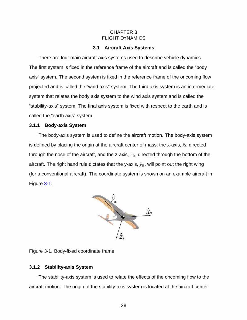
3.1.1 Body-axis System
The body-axis system is used to define the aircraft motion. The body-axis system
is defined by placing the origin at the aircraft center of mass, the x-axis, xB directed
through the nose of the aircraft, and the z-axis, zB , directed through the bottom of the
aircraft. The right hand rule dictates that the y-axis, yB , will point out the right wing
(for a conventional aircraft). The coordinate system is shown on an example aircraft in
Figure 3-1.
Figure 3-1. Body-fixed coordinate frame
3.1.2 Stability-axis System
The stability-axis system is used to relate the effects of the oncoming flow to the
aircraft motion. The origin of the stability-axis system is located at the aircraft center
28

of mass, but the x-axis, xS , points in the direction of projection of the wind onto the
xB zB-plane. Thus, the y-axis of the stability-axis system, yS , is coincidental with yB . The
angle of rotation that would align xS with xB and zS with zB is defined as the angle of
attack and is denoted by the symbol α, where α ∈ R. Figure 3-2 details the rotation
between the body-axis system and the stability-axis system.
Figure 3-2. Stability coordinate frame
The aerodynamic forces in the stability-axis system are given conventional names.
The aerodynamic force in the negative xS direction is called the drag and is represented
by the variable, D. The aerodynamic force in the positive yS direction is called the
sideforce and is represented by the variable, Y . The aerodynamic force in the negative
zS direction is called the lift and represented by the variable, L. These relations are
shown in Equation 3–1.
D
Y
L
S
,
−FAerox
FAeroy
−FAeroz
S
(3–1)
where, FAeroi = aerodynamic force in i direction
for i = x , y , z
29

3.1.3 Wind-axis System
The wind-axis system also has its origin at the aircraft center of mass, but its
x-axis, xW , is directed into the oncoming flow. The wind-axis system is related to the
stability-axis system by a coordinate system rotation. The body-axis system is rotated
by the angle of sideslip, β, about zs . Figure 3-3 shows the relationship between the
wind-axis and the stability-axis system.
Figure 3-3. Wind coordinate frame
3.1.4 Earth-axis System
The earth-axis system is used to include gravitational effects on the aircraft motion.
The origin of the earth-axis system is located at the surface of the earth and the z-axis,
zE , points toward the center of the earth. The exact direction of the x- and y-axes, xE
and yE , is arbitrary as long as they form an orthogonal set with zE . Figure 3-4 illustrates
the differences in both rotation and translation between the earth-axis system and the
body-axis system.
3.2 Coordinate Transformations
Mathematical relations are established between the axis systems of Section 3.1
to relate the dynamic effects on the aircraft due to forces in other axis systems. These
relations are stated in a coordinate rotation framework whereby one vector can be
multiplied by an orthonormal matrix to find the vector in the coordinates of a second axis
30

Figure 3-4. Earth-fixed coordinate frame
system. This mathematical relation is stated in Equation 3–2, where X is the original
vector, X ′ is the rotated vector, and the rotation matrix R relates the two.
X ′ = RX (3–2)
where, X ,X ′ ∈ Rn
R ∈ Rnxn
3.2.1 Wind to Stability Frame
The relation between the wind-axis system and the stability-axis system is a rotation
about zW by an angle β. This angle is important when examining the lateral dynamics
of the aircraft. The relation of the aerodynamic forces in the two systems is shown in
Equation 3–3.
31

FAerox
FAeroy
FAeroz
S
=
cos β sinβ 0
− sin β cos β 0
0 0 1
FAerox
FAeroy
FAeroz
W
(3–3)
3.2.2 Stability to Body Frame
The relation between the stability-axis system and the body-axis system is a
rotation about yS by the angle of attack, α. This angle is important when examining the
longitudinal dynamics of the aircraft. The relation of the aerodyamic forces in the two
systems is shown in Equation 3–4.
FAerox
FAeroy
FAeroz
B
=
cosα 0 − sinα
0 1 0
sinα 0 cosα
−D
Y
−L
S
(3–4)
3.2.3 Earth to Body Frame
The relation between the earth-fixed frame and the body-fixed frame is a rotation
followed by a translation, but the translation is unnecessary for the purposes of relating
forces between the two frames. So, rotations need to be defined that transform the
orientation of the earth-fixed frame to that of the body-fixed frame. These rotations can
be defined in multiple ways, but the conventional 3-2-1 transformation is described here.
By convention, this transformation requires the rotation about the z-axis to be done first,
followed by a rotation about the transformed y-axis, and finally, a rotation about the new
transformed x-axis. The angles used in the rotations are called the Euler angles and
are conventionally defined such that: the yaw angle, ψ, is the angle of rotation about
the z-axis, the pitch angle, θ, is the rotation about the y-axis, and the roll angle, φ, is the
rotation about the x-axis.
32

In the process of transformation between the earth-fixed frame and the body-fixed
frame, intermediate coordinate systems, 1 and 2, will be defined. These are used simply
for explanatory purposes and will not be used again.
The first rotation is done about zE by angle ψ, as shown in Figure 3-5.
Figure 3-5. Rotation through ψ
This rotation transforms the axes in the earth-fixed frame to axes in intermediate
frame 1 by applying Equation 3–5.
x
y
z
1
= R3(ψ)
x
y
z
E
=
cosψ sinψ 0
− sinψ cosψ 0
0 0 1
x
y
z
E
(3–5)
The second rotation is done about y1 by angle θ, as shown in Figure 3-6.
This rotation transforms the axes in intermediate frame 1 to axes in intermediate
frame 2 by applying Equation 3–6.
x
y
z
2
= R2(θ)
x
y
z
1
=
cos θ 0 − sin θ
0 1 0
sin θ 0 cos θ
x
y
z
1
(3–6)
The third rotation is done about x2 by angle φ, as shown in Figure 3-7.
33

Figure 3-6. Rotation through θ
Figure 3-7. Rotation through φ
The rotation transforms the axes in intermediate frame 2 to axes in the body-fixed
frame by applying Equation 3–7.
x
y
z
B
= R1(φ)
x
y
z
2
=
1 0 0
0 cosφ sin φ
0 − sin φ cosφ
x
y
z
2
(3–7)
Equation 3–8 shows how the rotations can be combined to provide a one step
process that orients the earth-fixed axes with the body-fixed axes.
34

x
y
z
B
= R1(φ)R2(θ)R3(ψ)
x
y
z
E
(3–8)
Thus, any vector in earth-fixed coordinates, vE , can be expressed in body-fixed
coordinates as vB by using the relationship in Equation 3–9.
vB =
cos θ cosψ sin φ sin θ cosψ − cosφ sinψ cos φ sin θ cosψ + sinφ sinψ
cos θ sinψ sin φ sin θ sinψ + cosφ cosψ cos φ sin θ sinψ − sinφ cosψ
− sin θ sinφ cos θ cos φ cos θ
vE (3–9)
For example, the gravitational force is expressed in both earth-fixed and body-fixed
coordinates in Equation 3–10.
FGrav =
0
0
mg
E
=
−mg sin θ
mg sinφ cos θ
mg cosφ sin θ
B
(3–10)
3.3 Nonlinear Equations of Motion
3.3.1 Dynamic Equations
The rigid body equations of motion are derived from Newton’s second law, which
holds true in inertial reference frames. The only inertial reference frame that is defined
in Section 3.2 is the earth-fixed reference frame; so, the dynamic equations are
derived in the earth-fixed reference frame. Newton’s second law is applied to forces
in Equation 3–11 and equates the sum of external forces to the time rate of change
of momentum of the body. When applied to moments in Equation 3–12, Newton’s
second law equates the sum of external moments to the time rate of change of angular
momentum.
35

∑
F =d
dt(mv)E (3–11)
∑
M =d
dtHE (3–12)
3.3.1.1 Force Equations
For the aerospace systems investigated in this research, the mass of the aircraft
can be assumed to be constant. This assumption permits a simplification of Equation 3–11,
expressed in Equation 3–13.
∑
F = md
dtvE = maE (3–13)
Note that to apply Equation 3–13, the acceleration in the earth-fixed frame, aE must
be known. The difficulty is that the accelerations are often measured in the body-fixed
frame; thus, the acceleration in the earth-fixed frame must be found using the transport
theorem, which is stated in Equation 3–14. The transport theorem relates the time rate
of change of a vector in one reference frame to the time rate of change of that vector in
another reference frame using the angular velocity between the two reference frames,
1ω2.
db
dt
∣
∣
∣
∣
1
=db
dt
∣
∣
∣
∣
2
+ 1ω2 × b (3–14)
Note that two properties hold true for angular rate vectors, ω, permitting conversion
between many different reference frames.
1ω2 = −2ω1 (3–15)
1ωn = 1ω2 + 2ω3 + ... + n−1ωn (3–16)
36

The velocity of an aircraft in the earth-fixed reference frame can be expressed in
body-fixed coordinates, and is defined in Equation 3–17.
vEB = uiB + v jB + wkB =
u
v
w
B
(3–17)
The angular velocity between the earth-fixed and body-fixed reference frames can
be expressed in body-fixed coordinates, and is defined in Equation 3–18.
EωB = piB + qjB + r kB =
p
q
r
B
(3–18)
To find the acceleration of an aircraft in the earth-fixed reference frame, the
transport theorem is applied to the earth- and body-fixed reference frames in Equation 3–19.
aEB =dvEBdt
∣
∣
∣
∣
E
=dvEBdt
∣
∣
∣
∣
B
+ EωB × vEB (3–19)
The right side of Equation 3–19 can be reduced to solve for the acceleration of the
aircraft as viewed by an observer in an earth-fixed reference frame, but expressed in
body-fixed coordinates. The resulting relationship is shown in Equation 3–20.
aEB =
u + qw − rv
v + ru − pw
w + pv − qu
B
(3–20)
Now that the right hand side of Equation 3–13 has been solved, the left hand side
must be defined. It is assumed that the only three types of forces that act on the aircraft
are gravitational, aerodyamic, and thrust forces; thus, resulting in a sum of external
forces that takes the form shown in Equation 3–21.
37

∑
F =
Fx
Fy
Fz
B
=
FGravx + FAerox + FThrustx
FGravy + FAeroy + FThrusty
FGravz + FAeroz + FThrustz
B
(3–21)
Recall the gravitational forces expressed in the body-fixed coordinates from
Equation 3–10 and the aerodynamic forces expressed in the body-fixed coordinates
from Equation 3–4. When those relationships and Equation 3–20 are applied to
Equation 3–13, three equations result, as shown in Equations 3–22 - 3–24.
m(u + qw − rv) = −mg sin θ + (−D cosα+ L sinα) + FThrustx (3–22)
m(v + ru − pw) = mg sin φ cos θ + Y + FThrusty (3–23)
m(w + pv − qu) = mg cos φ cos θ + (−D sinα− L cosα) + FThrustz (3–24)
3.3.1.2 Moment Equations
Referring back to Equation 3–12, the angular momentum in the earth-fixed
reference frame expressed in body-fixed coordinates, HEB , is the product of the inertia
tensor, IB, and the angular velocity vector, EωB . This relationship is expressed in
Equation 3–25.
HEB = IB
EωB (3–25)
The inertia tensor, IB, can be defined as in Equation 3–26.
IB =
Ixx −Ixy −Ixz
−Iyx Iyy −Iyz
−Ixz −Iyz Izz
B
(3–26)
Thus, using the definitions in Equation 3–26 and Equation 3–18, the angular
momentum can be expressed as in Equation 3–27.
38

HEB =
Ixx −Ixy −Ixz
−Iyx Iyy −Iyz
−Ixz −Iyz Izz
B
P
Q
R
B
=
pIx − qIxy − rIxz
qIy − rIz − pIxy
rIz − pIxz − qIyz
B
(3–27)
Note that the angular momentum is expressed in body-fixed coordinates; so, the
transport theorem in Equation 3–14 will need to be applied to find the rate of change of
the angular momentum in the earth-fixed reference frame. The transport theorem, as
applied to the angular momentum, is stated in Equation 3–28.
dHEB
dt
∣
∣
∣
∣
E
=dHE
B
dt
∣
∣
∣
∣
B
+ EωB ×HEB (3–28)
The first term on the right hand side of Equation 3–28 is simple to calculate and is
further simplified by assuming that the moment of inertia, IB, is constant. The result is
expressed in Equation 3–29.
dHEB
dt
∣
∣
∣
∣
B
=
pIx − qIxy − r Ixz
qIy − r Iyz − pIxy
r Iz − pIxz − qIyz
B
(3–29)
The second term on the right side of Equation 3–28 is expressed in Equation 3–30.
EωB ×HEB =
qrIz − qpIxz − q2Iyz − qrIy + r
2Iyz + rpIxy
rpIx − qrIxy − r2Ixz − rpIz + p
2Ixz + qpIyz
pqIy − rpIyz − p2Ixy − pqIx + q
2Ixy + rqIxz
(3–30)
Combining the results of Equations 3–28, 3–29, and 3–30, the time rate of change
of angular momentum in an earth-fixed reference frame can be expressed as in
Equation 3–31.
39

d
dtHE =
dHEB
dt
∣
∣
∣
∣
E
=
pIx − qIxy − r Ixz + qrIz − qpIxz − q2Iyz − qrIy + r
2Iyz + rpIxy
qIy − r Iyz − pIxy + rpIx − qrIxy − r2Ixz − rpIz + p
2Ixz + qpIyz
r Iz − pIxz − qIyz + pqIy − rpIyz − p2Ixy − pqIx + q
2Ixy + rqIxz
B
(3–31)
Now that the right hand side of Equation 3–12 has been solved, the left hand side
must be defined. The sum of external moment that act on an aircraft is defined simply as
three moments that act about each of the principal body axes; thus, resulting in a sum of
external moments that takes the form shown in Equation 3–32.
∑
M =
Mx
My
Mz
B
=
L
M
N
B
=
LAero + LThrust
MAero +MThrust
NAero + NThrust
B
(3–32)
Equations 3–32 and 3–31 can be substituted into Equation 3–12 to yield Equations 3–33
- 3–35 that express the rotational dynamics of an aircraft in flight.
L = pIx − qrIy + qrIz + (pr − q)Ixy − (pq + r)Ixz + (r2 − q2)Iyz (3–33)
M = prIx + qIy − prIz − (qr − p)Ixy + (p2 − r2)Ixz + (pq − r)Iyz (3–34)
N = −pqIx + pqIy + r Iz + (q2 − p2)Ixy + (qr − p)Ixz − (pr + q)Iyz (3–35)
3.3.2 Kinematic Equations
Equations 3–22 - 3–24 and 3–33 - 3–35 do not completely describe the aircraft
dynamics. Six more equations are required to fully describe the aircraft dynamics; these
six equations are provided by the aircraft kinematics.
3.3.2.1 Orientation Equations
Three equations can be found by recognizing that the rotation of the body-fixed
frame relative to the earth-fixed frame in body-fixed coordinates can be expressed in
40

another coordinate system. This relation is stated in Equation 3–36 and is derived from
the fact that a vector expressed in one coordinate system can be expressed in any other
coordinate system.
BωEB =BωE (3–36)
Expanding the two terms of Equation 3–36 using the coordinate systems of
Section 3.2 yields Equation 3–37.
piB + qjB + r kB = φi + θj + ψkE (3–37)
Note that the x-axis of the body frame is shared by reference frame 2, the y-axis
of reference frame 1 is shared by reference frame 2, and the z-axis of the earth-fixed
reference frame is shared by reference frame, so Equation 3–37 can be rewritten as
Equation 3–38.
piB + qjB + r kB = φiB + θj + ψk (3–38)
The coordinate transformations of Section 3.2 can be used to show relations
between the coordinates in the right hand side of Equation 3–38 and body fixed
coordinates. These relations are shown in Equations 3–39 and 3–40.
j = cosφjB + sinφkB (3–39)
k = − sin θiB + sinφ cos θjB + cos φ cos θkB (3–40)
These relations of Equations 3–39 and 3–40 are substituted into Equation 3–37 to
produce three equations, expressed in Equations 3–41 - 3–43.
41

p = φ− ψ sin θ (3–41)
q = θ cos φ+ ψ cos θ sin φ (3–42)
r = ψ cos θ cos φ− θ sin φ (3–43)
Equations 3–41 - 3–43 can be rewritten with the Euler angles on the left side of the
equations, as seen in Equations 3–44 - 3–46.
φ = p + q(sinφ+ r cos φ) tan θ (3–44)
θ = q cos φ− r sinφ (3–45)
ψ = (q sinφ+ r cos φ) sec θ (3–46)
3.3.2.2 Position Equations
The final three equations describe the position of the aircraft in an earth-fixed
reference frame but expressed in body-fixed coordinates, as defined in Equation 3–47.
x
y
z
E
B
=
dx/dt
dy/dt
dz/dt
E
B
(3–47)
In Equation 3–48 the right side of Equation 3–47 is expressed as the matrix product
of the velocities in the body-fixed reference frame and the inverse of the transformation
matrix used in Equation 3–9.
dx/dt
dy/dt
dz/dt
E
B
=
cos θ cosψ sin φ sin θ cosψ − cosφ sinψ cos φ sin θ cosψ + sinφ sinψ
cos θ sinψ sin φ sin θ sinψ − cosφ cosψ cos φ sin θ sinψ + sinφ cosψ
− sin θ sin φ cos θ cosφ cos θ
u
v
w
B
(3–48)
42

Thus, the three equations describing the velocity in an earth-fixed reference frame
result. These equations are separated and stated in Equations 3–49 - 3–51.
xEB = u cos θ cosψ + v(sinφ sin θ cosψ − cos φ sinψ) + w(cos φ sin θ cosψ + sinφ sinψ)
(3–49)
yEB = u cos θ sinψ + v(sinφ sin θ sinψ + cos φ cosψ) + w(cos φ sin θ sinψ − sinφ cosψ)
(3–50)
zEB = −u sin θ + v(sin φ cos θ) + w cos φ cos θ (3–51)
3.3.3 The Equations Collected
The nonlinear aircraft equations of motion can be collected into a formal set, as
shown in Equation 3–52.
43

m(u + qw − rv) = −mg sin θ + (−D cosα+ L sinα) + FThrustx
m(v + ru − pw) = mg sin φ cos θ + Y + FThrusty
m(w + pv − qu) = mg cos φ cos θ + (−D sinα− L cosα) + FThrustz
L = pIx − qrIy + qrIz + (pr − q)Ixy − (pq + r)Ixz + (r2 − q2)Iyz
M = prIx + qIy − prIz − (qr − p)Ixy + (p2 − r2)Ixz + (pq − r)Iyz
N = −pqIx + pqIy + r Iz + (q2 − p2)Ixy + (qr − p)Ixz − (pr + q)Iyz
φ = p + q(sinφ+ r cos φ) tan θ (3–52)
θ = q cosφ− r sin φ
ψ = (q sinφ+ r cos φ) sec θ
xEB = u cos θ cosψ + v(sinφ sin θ cosψ − cosφ sinψ) + w(cosφ sin θ cosψ + sin φ sinψ)
yEB = u cos θ sinψ + v(sinφ sin θ sinψ − cos φ cosψ) + w(cosφ sin θ sinψ + sin φ cosψ)
zEB = −u sin θ + v(sinφ cos θ) + w cosφ cos θ
3.4 Linearized Equations of Motion
The nonlinear equations in Equation 3–52 are complicated and highly coupled.
Often, the coupled and nonlinear terms are dominated by the uncoupled linear terms;
thus, a linear set of equations can be a much more powerful tool in predicting and
controlling the motion of an aircraft. The equations are linearized using small-disturbance
theory, whereby a standard operating condition for all states is given, and any deviations
about that operating condition are assumed to be small. The results of applying
equations obtained using this assumption will deteriorate as the true operating condition
deviates from the assumed standard operation condition.
The states and moments of Equation 3–52 are expressed as a sum of a reference
value, (·)o, and a perturbation, ∆(·), in Equation 3–53.
44

u = uo +∆u
p = po +∆p
x = xo +∆x
M = Mo +∆M
L = Lo +∆L
v = vo +∆v
q = qo +∆q
y = yo +∆y
N = No +∆N
D = Do +∆D
w = wo +∆w
r = ro +∆r
z = zo +∆z
L = Lo +∆L
Y = Yo +∆Y
(3–53)
The most common reference condition to linearize about is that of steady level flight.
Equation 3–54 shows the reference conditions that can assumed to be zero in steady
level flight for a left-right symmetric aircraft.
vo = wo = po = qo = ro = φo = ψo = 0 (3–54)
Additionally, a small angle assumption will be made that the longitudinal velocity, uo ,
is equal to the reference flight speed. Trigonometric identities, shown in Equation 3–55,
can be applied when substituting Equation 3–53 into Equation 3–52.
sin(θo +∆θ) = sin θo cos∆θ + cos θo sin∆θ.= sin θo +∆θ cos θo
cos(θo +∆θ) = cos θo cos∆θ − sin θo sin∆θ.= cos θo −∆θ sin θo
(3–55)
The result of combining Equations 3–52 - 3–55 and eliminating all higher order
terms is shown in Equation 3–56.
45

(−D cosα+ L sinα) + FThrustx −mg(sin θo +∆θ cos θo) = m∆u
Y + FThrusty +mgφ cos θo = m(∆v + uo∆r)
(−D sinα− L cosα) + FThrustz +mg(cos θo −∆θ sin θo) = m(∆w − uo∆q)
∆L = Ix∆p − Izx∆r
∆M = Iy∆q
∆N = −Izx∆p + Iz∆r
θo +∆θ = ∆q
φo +∆φ = ∆p +∆r tan θo
ψo +∆ψ = ∆r sec θo
xEo +∆xE = (uo +∆u) cos θo − uo∆θ sin θo +∆w sin θo
yEo +∆yE = uoψ cos θo +∆v
zEo +∆zE = −(uo +∆u) sin θo − uo∆θ cos θo +∆w cos θo
(3–56)
If all of the disturbances in Equation 3–56 are set to zero, then the resulting
Equation 3–57 shows the equalities of the reference flight condition.
Xo −mg sin θo = 0
Yo = 0
Zo +mg cos θo = 0
Lo = Mo + No = 0
xEo = uo cos θo
yEo = 0
zEo = −uo sin θo
(3–57)
Equation 3–57 is substituted into Equation 3–56, so that the linearized motion
equations can be rewritten as Equation 3–58.
46

∆u = ∆xm
− g∆θ cos θo
∆v = ∆ym+ g∆φ cos θo − uo∆r
∆w = ∆zm
− g∆θ sin θo + uo∆q
∆L = Ix∆p − Izx∆r
∆M = Iy q
∆N = −Izx∆p + Iz∆r
∆θ = ∆q
∆φ = ∆p +∆r tan θo
∆ψ = ∆r sec θo
∆xE = ∆u cos θo − uo∆θ sin θo +∆w sin θo
∆yE = uo∆ψ cosΘo − v
∆zE = −∆u sin θo − uo∆θ cos θo +∆w cos θo
(3–58)
The perturbation terms of aerodynamic forces and moments in Equation 3–58 can
be expressed as a Taylor series expansion. For example, the perturbation term of the
aircraft roll moment can be expressed as in Equation 3–59.
∆L =∂L
∂u∆u +
∂L
∂v∆v +
∂L
∂w∆w +
∂L
∂q∆q +
∂L
∂p∆p +
∂L
∂r∆r +
∂L
∂δa∆δa +
∂L
∂δr∆δr +
∂L
∂δe∆δe
(3–59)
The partial derivatives in this first order Taylor series expansion form the basis of a
linear analysis of aircraft dynamics. These terms represent the sensitivity of the aircraft
to changes in the aircraft states. Important partial derivative terms include: Lα (the
sensitivity of lift to changes in angle of attack), MYα(the sensitivity of pitch moment to
changes in angle of attack, which is indicative of the longitudinal stability of the aircraft),
MXβ(the sensitivity of roll moment to changes in the angle of sideslip, which is indicative
of the roll stability of the aircraft), MZβ (the sensitivity of yaw moment to changes in
47

the angle of sideslip, which is indicative of the yaw stability of the aircraft), and Yβ (the
sensitivity of sideforce to changes in the angle of sideslip).
48
CHAPTER 4WIND TUNNEL TESTING
It is well understood from the previous chapters that neither aircraft nor turbulence
are strictly linear dynamical systems. For some purposes linearity can be a sufficient
approximation. It is in this frame of mind that traditional linear flight control has treated
turbulent fluctuations as perturbations with respect to a trim state. Doing so assumes
that small positive changes in the velocity components will have a symmetric effect
with respect to small negative changes. However, the research conducted herein
hypothesizes that this assumption is incorrect.
Wind tunnel testing is conducted to understand the interactions of turbulence and
micro air vehicle (MAV) flight dynamics. Two sets of tests are conducted; each in a
different research location using different vehicles, test matrices, and measurement
procedures. Both tests use grids to generate the turbulence that impacts the aircraft
dynamics.
The first set of tests are referred to as static tests because they keep the vehicle
stationary in the flow and examine only the relationships between the flight angles,
turbulence intensity, and symmetric wing sweep angle. In these tests the model is
assumed to have linear dynamics, and the static stability coefficients are time averaged
during long test runs under both smooth and turbulent flow conditions. The static
stability derivatives are hypothesized to differ significantly between both smooth and
turbulent flow, proving that the presence of turbulence introduces new terms in the
equations representing the flight dynamics of MAVs. To test this hypothesis, the forces
and moments are found at varying angles of attack and sideslip in flows of different
turbulence intensities, and the force and moment derivatives with respect to those flight
angles are calculated.
The second set of tests are referred to as dynamic tests because they increase the
number of parameters in the test matrix by including pitching and plunging maneuvers.
49

The second set of tests also include the effects of symmetric wing dihedral. In these
tests, the model is assumed to have nonlinear dynamics of a quadratic form. In
other words, all states or parameters that are included in the model have all linear,
quadratic, and associated cross-coupling terms included. Of particular importance are
the cross-coupling terms between turbulence intensity and other states. These tests
intend to show new mathematical terms to represent the effect of turbulence on MAV
dynamics.
4.1 Static Wind Tunnel Testing
4.1.1 Wind Tunnel Setup
Static wind tunnel data is found using the Royal Melbourne Institute of Technology
(RMIT) Industrial Wind Tunnel (IWT). The IWT is a 2m x 3m closed jet, closed test
section wind tunnel.
Turbulence is produced by a set of grids, seen in Figure 4-1, placed upstream of the
contraction to the tunnel test section. The model is mounted near the expansion end of
the test section (9m from the grids, which is greater than 10 times the width of the grid
elements) to allow the turbulence to become well mixed and homogeneous. The wind
tunnel has an inherent turbulence intensity of 1.2% at the model when the grids are not
installed, and a turbulence level of 7.4% when the grids are installed [105]. These grids
have been shown to produce turbulence similar to that present in the ABL [105].
As shown in Figure 4-2, the MAV is mounted down the wind tunnel center line. The
model is attached to a vertical mounting rod, which attaches to the 6 degree of freedom
JR3 100M40A force balance. The bottom of the balance is attached to a sting that bolts
to the wind tunnel floor. A pitot tube is located just below the right wing leading edge.
Experiments are conducted with the “Flash” commercially available expanded
polypropylene (EPP) foam MAV. The model has an aft-placed tail, mid wing design, and
fuselage with a rectangular cross-section. The factory standard wings are replaced with
hotwire cut EPP foam wings. The wings use a NACA 2410 airfoil and are designed to
50

Figure 4-1. Turbulent setup in RMIT industrial wind tunnel (Photo courtesy of BrianRoberts)
hold as many parameters constant as possible, while varying the leading edge sweep.
Wingspan (0.8 m), wing area (0.2 m2), root chord length (0.3 m), taper ratio (0.67), and
aspect ratio (0.8) are all held constant. The propeller and motor are also removed to
eliminate propeller downwash, but the pushrods and servos used for flight control are
left on the model.
The foam model shows noticeable vibration in turbulent flow. As a result, the
wingtips and control surfaces are stiffened using wire in both smooth and turbulent flow
tests. Copper wire is used to connect: 1) the wingtips (at the quarter chord point) to
the fuselage to reduce wing bending, 2) each side of the rudder to the top and bottom
surfaces of the elevator to reduce control surface deflections, and 3) the wingtips to the
tips of the horizontal tail to reduce fuselage twisting.
4.1.2 Experimental Design
The test matrix to find the aircraft stability derivatives includes 5 angles of attack
(-5, 0, 5, 10, 15) at 4 angles of sideslip (0, -3, -6, -9). The angles of attack are
measured using an inclinometer, and the angles of sideslip are measured by dropping
a plumb line from the tail and measuring the distance from the centerline of the wind
51

Figure 4-2. Test setup in RMIT industrial wind tunnel (Photos courtesy of Brian Roberts)
tunnel. This set of 20 data points is measured on both a swept (10 at leading edge)
and unswept (0 at leading edge) wing under both smooth and turbulent wind tunnel
conditions. The wind tunnel conditions are characterized by previous research with
smooth flow at 1.2% turbulence and the turbulent flow testing at 7.4% turbulence [105].
The test procedure is designed to yield accurate average forces and moments in
the presence of an observed sensor drift. The balance is tared at the start of each test
run, followed by an immediate ramping of the wind tunnel average airspeed to 8.3 m/s.
A five second averaged measurement is taken, followed by a two minute averaged
measurement, and then another five second measurement. At this point the power
to the wind tunnel turbine is turned off and a final five second measurement is taken.
The three short measurements are then used to find the rates of drift and the average
amount of drift present during the two minute test. Once the two minute measurement
has been corrected for drift, it is ready to be plotted.
4.1.3 Results
The three forces and three moments are shown for both swept and unswept wings
in both smooth flow (1.2% turbulence intensity) and turbulent flow (7.4% turbulence
intensity) in Figures 4-3−4-6.
52

−5051015
−10
−5
0
0
0.5
1
1.5
2
2.5
Beta (deg)
Alpha (deg)
Dra
g (N
)
−5051015−10
−50
−0.5
0
0.5
1
1.5
Beta (deg)
Alpha (deg)
Sid
efor
ce (
N)
−50
510
15
−10
−5
0−5
0
5
10
Alpha (deg)Beta (deg)
Lift
(N)
−5051015−10
−50
−0.1
0
0.1
0.2
0.3
Beta (deg)
Alpha (deg)
Mx
(Nm
)
−5 0 5 10 15 −10−5
0−0.4
−0.2
0
0.2
0.4
0.6
Beta (deg)
Alpha (deg)
My
(Nm
)
−5 0 5 10 15 −10−5
0−0.35
−0.3
−0.25
−0.2
−0.15
−0.1
−0.05
0
Beta (deg)
Alpha (deg)
Mz
(Nm
)
Figure 4-3. Unswept wing model in smooth flow
−5051015
−10
−5
0
0.5
1
1.5
2
2.5
3
3.5
Beta (deg)
Alpha (deg)
Dra
g (N
)
−5051015−10
−50
−0.5
0
0.5
1
1.5
2
Beta (deg)
Alpha (deg)
Sid
efor
ce (
N)
−50
510
15
−10
−5
0−5
0
5
10
15
Alpha (deg)Beta (deg)
Lift
(N)
−5051015−10
−50
−0.1
0
0.1
0.2
0.3
0.4
Beta (deg)
Alpha (deg)
Mx
(Nm
)
−5 0 5 10 15 −10−5
0−0.2
−0.1
0
0.1
0.2
0.3
0.4
0.5
Beta (deg)
Alpha (deg)
My
(Nm
)
−5 0 5 10 15 −10−5
0−0.4
−0.3
−0.2
−0.1
0
0.1
Beta (deg)
Alpha (deg)
Mz
(Nm
)
Figure 4-4. Unswept wing model in turbulent flow
Linearization of flight systems about an operation point is an accepted method to
gain insight to the flight dynamics; however, the system needs to be proven linear about
the design point. So, linear regression is performed on each subset of data, and the
validity of using a linear model for its dynamics is evaluated using the normalized root
mean square deviation of the experimental data from the model’s predicted data values.
The normalized root mean square deviation is a standard metric used to judge the
53

−5051015
−10
−5
0
0.5
1
1.5
2
2.5
3
3.5
Beta (deg)
Alpha (deg)
Dra
g (N
)
−5051015−10
−50
−0.5
0
0.5
1
1.5
2
Beta (deg)
Alpha (deg)
Sid
efor
ce (
N)
−50
510
15
−10
−5
0−5
0
5
10
15
Alpha (deg)Beta (deg)
Lift
(N)
−5051015−10
−50
−0.1
0
0.1
0.2
0.3
0.4
Beta (deg)
Alpha (deg)
Mx
(Nm
)
−5 0 5 10 15 −10−5
0−0.5
0
0.5
Beta (deg)
Alpha (deg)
My
(Nm
)
−5 0 5 10 15 −10−5
0−0.35
−0.3
−0.25
−0.2
−0.15
−0.1
−0.05
0
Beta (deg)
Alpha (deg)
Mz
(Nm
)
Figure 4-5. 10 Swept wing model in smooth flow
−5051015
−10
−5
0
0.5
1
1.5
2
2.5
3
3.5
Beta (deg)
Alpha (deg)
Dra
g (N
)
−5051015−10
−50
−0.5
0
0.5
1
1.5
2
Beta (deg)
Alpha (deg)
Sid
efor
ce (
N)
−50
510
15
−10
−5
0−5
0
5
10
15
Alpha (deg)Beta (deg)
Lift
(N)
−5051015−10
−50
−0.1
0
0.1
0.2
0.3
0.4
Beta (deg)
Alpha (deg)
Mx
(Nm
)
−5 0 5 10 15 −10−5
0−0.2
−0.1
0
0.1
0.2
0.3
0.4
0.5
Beta (deg)
Alpha (deg)
My
(Nm
)
−5 0 5 10 15 −10−5
0−0.4
−0.3
−0.2
−0.1
0
0.1
Beta (deg)
Alpha (deg)
Mz
(Nm
)
Figure 4-6. 10 Swept wing model in turbulent flow
quality of fit for a model []. The formula for the normalized root mean square deviation is
given in Equation 4–1.
NRMSD(θexp, θmodel) =
√∑ni=1(θexp,i−θmodel ,i)2
n
θexpmax − θexpmin(4–1)
The normalized root mean square deviations for select moment and force
derivatives are shown in Tables 4-1-4-5. Analyzing normalized root mean square
54

deviations can be rather arbitrary, but the vast majority of values are below 5%, and the
values under high values of turbulence show no significant increases, which indicates
that the linear force and moment derivatives under turbulence are just as useful as those
taken in low turbulence.
Table 4-1. Normalized root mean square deviation for Lα
Test Conditions β = 0 β = 3 β = 6 β = 9
α = 15
ΛLE = 0, I = 1.2% 2.99% 3.96% 4.48% 3.47%ΛLE = 10, I = 1.2% 3.55% 12.18% 3.04% 3.78%ΛLE = 0, I = 7.4% 3.35% 2.70% 4.32% 3.89%ΛLE = 10, I = 7.4% 2.37% 3.07% 3.90% 2.71%
Table 4-2. Normalized root mean square deviation for MYα
Test Conditions β = 0 β = 3 β = 6 β = 9
α = 15
ΛLE = 0, I = 1.2% 7.63% 15.80% 15.41% 17.39%ΛLE = 10, I = 1.2% 7.99% 8.41% 5.64% 8.26%ΛLE = 0, I = 7.4% 8.63% 7.85% 13.72% 7.68%ΛLE = 10, I = 7.4% 15.45% 10.46% 13.41% 17.13%
Table 4-3. Normalized root mean square deviation for Yβ
Test Conditions α = -5 α = 0 α = 5 α = 10 α = 15
ΛLE = 0, I = 1.2% 4.97% 4.43% 4.19% 1.94% 3.23%ΛLE = 10, I = 1.2% 2.28% 1.68% 5.10% 2.44% 3.30%ΛLE = 0, I = 7.4% 2.43% 1.59% 1.88% 3.02% 3.38%ΛLE = 10, I = 7.4% 3.82% 3.59% 5.17% 3.22% 3.50%
Table 4-4. Normalized root mean square deviation for MXβ
Test Conditions α = -5 α = 0 α = 5 α = 10 α = 15
ΛLE = 0, I = 1.2% 3.60% 1.81% 3.07% 1.56% 5.99%ΛLE = 10, I = 1.2% 2.70% 3.87% 4.38% 4.01% 8.96%ΛLE = 0, I = 7.4% 2.04% 2.20% 2.85% 4.47% 4.29%ΛLE = 10, I = 7.4% 8.39% 3.67% 7.15% 4.58% 4.56%
The lift force and pitch moment show a strong linear correlation with the angle
of attack (α), and the sideforce, roll moment, and yaw moment show a strong linear
55

Table 4-5. Normalized root mean square deviation for MZβ
Test Conditions α = -5 α = 0 α = 5 α = 10 α = 15
ΛLE = 0, I = 1.2% 5.11% 7.32% 4.86% 2.34% 5.51%ΛLE = 10, I = 1.2% 3.24% 1.88% 5.76% 3.32% 5.24%ΛLE = 0, I = 7.4% 3.26% 2.64% 0.40% 4.94% 4.71%ΛLE = 10, I = 7.4% 3.98% 2.02% 7.36% 5.04% 4.85%
correlation with the angle of sideslip (β). The data demonstrates strong linear trends,
so the slopes of these linear tendencies are compared over amounts of sweep and
turbulence. The slopes are found at each flight angle, averaged, and shown with their
standard deviation. For example, the derivative of lift with respect to angle of attack is
found by running a linear correlation, in the least squares sense, on the data at each of
the four angles of sideslip, as shown in Figure 4-7 using the data from the unswept wing
in smooth flow.
56

−5 0 5 10 15−2
0
2
4
6
8
10
Alpha (deg)
Lift
(N)
−5 0 5 10 15−2
0
2
4
6
8
10
Alpha (deg)
Lift
(N)
−5 0 5 10 15−2
0
2
4
6
8
10
Alpha (deg)
Lift
(N)
−5 0 5 10 15−4
−2
0
2
4
6
8
10
Alpha (deg)
Lift
(N)
Figure 4-7. Lift curves at each sideslip angle
(solid line for experimental data, dashed line for linear regression, β=0 top left, β=-3 topright, β=-6 bottom left, β=-9 bottom right)
57

The four slopes are averaged to give a mean slope for the surface and the standard
deviation is also found, as shown in Table 4-6.
Table 4-6. Finding mean slope and standard deviation
β Lift Curve Slope (N/)0 0.5210-3 0.5439-6 0.5111-9 0.5496Mean 0.5134σ 0.0183
The mean slopes and standard deviations for both forces and moments under all
test conditions are shown in Tables 4-7–4-11.
Table 4-7 shows the lift curve slope. The lift curve slope is defined in Equation 4–2.
Lα =∂L
∂α(4–2)
Table 4-7. Lα average derivatives and standard deviations (N/)
1.2% Turbulence 7.4% Turbulence0 Sweep 0.531 ± 0.018 0.722 ± 0.02410 Sweep 0.660 ± 0.055 0.679 ± 0.031
According to Table 4-7, in the absence of turbulence, the addition of 10 wing
sweep produces a 24% increase in the production of lift due to an increase in the angle
of attack. In the presence of turbulence, a decrease of 6.0% in the lift curve slope is
observed as the wing is swept; however, this difference in means is not large enough
to be outside the bounds of the one-sigma ranges of the two values. The presence of
turbulence produced a 36% increase in the production of lift due to an increase in the
angle of attack for an unswept wing, but produced an insignificant (2.8% and not outside
the bounds of a one-sigma range) increase in lift production for a swept wing.
58

Table 4-8 shows the pitching moment curve slope. The pitching moment curve
slope, MYα, is also referred to as the longitudinal static stability derivative is defined in
Equation 4–3. A negative value indicates that it is statically stable about the lateral axis.
MYα=∂MY∂α
(4–3)
Table 4-8. MYαaverage derivatives and standard deviations (Nm/)
1.2% Turbulence 7.4% Turbulence0 Sweep -0.0247 ± 0.0025 -0.0191 ± 0.003610 Sweep -0.0402 ± 0.0022 -0.0200 ± 0.0057
According to Table 4-8, in the absence of turbulence, the addition of 10 wing
sweep produces a 63% increase in the production of a negative pitch moment due to
an increase in the angle of attack. In the presence of turbulence, this increase is only
4.7% (a difference that lies within the one-sigma bounds). This observed trend does
not agree with some conventional expectations that sweep back of the wings changes
the downwash on the tail, and thus, reduces longitudinal stability [106]. However, it is
possible that the marginal change in sweep angle in the tests is not enough to create the
significant increase in the downwash on the tail that is associated with sweep induced
reduction of longitudinal stability. So, the dominant effect seen is an aftward movement
of the center of lift and resulting longitudinal stability improvements. The added sweep
moves the center of lift further aft of the center of gravity, increasing the static margin
and improving the longitudinal stability. The presence of turbulence produces a 23%
decrease in the production of a negative pitch moment due to an increase in the angle of
attack for an unswept wing. This decrease lies just within the one-sigma ranges for the
MYαslopes.
Table 4-9 shows the sideforce curve slope. The sideforce curve slope is defined in
Equation 4–4.
59

Yβ =∂Y
∂β(4–4)
Table 4-9. Yβ average derivatives and standard deviations (N/)
1.2% Turbulence 7.4% Turbulence0 Sweep -0.149 ± 0.011 -0.200 ± 0.009310 Sweep -0.164 ± 0.023 -0.205 ± 0.014
According to Table 4-9, in the absence of turbulence, the addition of 10 wing
sweep produces a 10% increase in the production of sideforce due to an increase in the
sideslip angle. In the presence of turbulence, this increase is only 2.5%. The presence
of turbulence produces a 34% increase in the production of sideforce due to a sideslip
angle for an unswept wing. However, it should be noted that the one-sigma ranges (the
range of values within one standard deviation of the mean) for the Yβ slopes overlap
each other when the turbulence intensity is held constant; thus, indicating that wing
sweep may have a negligible impact on Yβ in both smooth and turbulent flow.
Table 4-10 shows the roll moment curve slope. The roll moment curve slope,
MXβ, is also referred to as the roll moment static stability derivative, and is defined in
Equation 4–5. A negative value indicates that the vehicle is statically stable about the
longitudinal axis.
MXβ=∂MX∂β
(4–5)
Table 4-10. MXβaverage derivatives and standard deviations (Nm/)
1.2% Turbulence 7.4% Turbulence0 Sweep -0.0326 ± 0.0036 -0.0432 ± 0.004010 Sweep -0.0358 ± 0.0049 -0.0442 ± 0.0037
According to Table 4-10, in the absence of turbulence, the addition of 10 wing
sweep produces a 9.8% increase in the production of a negative rolling moment due
to an increase in the sideslip angle. The change in the mean MXβis not outside the
60

bounds of a one-sigma range. The presence of turbulence produces a 32% increase in
the production of a negative rolling moment due to an increase in the sideslip angle on
an unswept wing, and a 23% increase on a 10 swept wing.
Table 4-11 shows the yaw moment curve slope. The yaw moment curve slope,
MZβ , is also referred to as the yaw moment static stability derivative, and is defined in
Equation 4–6. A positive value indicates that the vehicle is statically stable about the
vertical axis.
MZβ =∂MZ∂β
(4–6)
Table 4-11. MZβ average derivatives and standard deviations (Nm/)
1.2% Turbulence 7.4% Turbulence0 Sweep 0.027 ± 0.0024 0.038 ± 0.002810 Sweep 0.030 ± 0.0051 0.038 ± 0.0027
According to Table 4-11, in the absence of turbulence, the addition of 10 wing
sweep produces a 11% increase in the production of a yaw moment due to an increase
in the angle of sideslip. In the presence of turbulence, no change is seen in MZβ as
sweep changes. Neither in turbulence, nor in smooth flow is a significant (outside of
one-sigma range) change seen with wing sweep. The presence of turbulence produces
a 41% increase in the production of yaw moment due to an increase in the angle of
sideslip for an unswept wing.
4.1.4 Analysis
The cause for the increase in the lift curve slope with wing sweep is somewhat
counterintuitive. In fact, the section lift coefficient is expected to decrease with
increasing sweep due to the reduction in the magnitude of the velocity that is perpendicular
to the wing [107]. If the wing is assumed to behave like a beam (the flexural axis is
always parallel to the sweep axis), then static aeroelastic effects also predict a reduction
in the lift curve slope with increasing sweep, because wing bending for a swept back
61

wing results in a reduced angle of incidence [108]. However, the wings used for testing
might have too low of an aspect ratio to apply the results of “beam-model” wings. The
wing vibration seen in the tests could cause an increase in the lift coefficient, because
the effective angle of incidence varies through the pitching and twisting movement [108].
The placement of the copper wire at the wing quarter chord might also increase the
effective angle of incidence, because the flexural axis for a swept wing lies aft of the
midchord [108].
The improvement in longitudinal static stability derivative, MYα, in the static tests can
be attributed to the increase in the lift curve slope and movement of the center of lift as
the wing is swept backwards. As the center of lift of the wing, xwing, moves backwards,
the neutral point, xnp, becomes moves backwards as well. This relationship is apparent
from Equation 4–7, which assumes small angles, that the aircraft is in a trim state, and
that fuselage effects are negligible.
(Lwing + Ltail +Dwing + Dtail)xnp = Lwingxwing +Dwingywing + Ltailxtail + Dtailytail (4–7)
There is a relationship between the neutral point, MYα, and Lα, shown in Equation 4–8.
The relationship indicates that as the neutral point moves backwards, and longitudinal
static stability increases. Equation 4–8 also indicates that if Lα increases, then MYα
increases proportionately.
MYα= xnpLα (4–8)
The longitudinal position of the neutral point on both the swept and unswept wings
is calculated according to Equation 4–9.
xnp =MYα
Lα(4–9)
62

The calculations in Equation 4–10 apply the lift curve slope and pitch moment slope
data for smooth flow in Tables 4-7 and 4-8 to show the position of the neutral point of the
unswept wing.
xnpunswept =−0.0247
0.531(4–10)
= 0.0465 m
The calculations in Equation 4–11 apply the lift curve slope and pitch moment slope
data for smooth flow in Tables 4-7 and 4-8 to show the position of the neutral point of the
swept wing.
xnpswept =−0.0402
0.660(4–11)
= 0.0610 m
Equation 4–12 shows that if the data is assumed to be correct, then the neutral
point would have moved 1.5 cm.
∆xnp = xnpswept − xnpunswept
= 0.0610 − 0.0465 (4–12)
= 0.0145 m
Thus, the dramatic increase in MYαcould be created by the combination of increase
in the lift curve slope and a movement of the neutral point of 1.5 cm.
It is impossible to tell the exact quantity of movement of the neutral point because
no measurements are made of the forces of the wing or tail independently. However,
calculations show that the aircraft neutral point could have moved up to 3.2cm.
63

Geometric properties lead to the derivation of Equations 4–13 to find the longitudinal
shift of the mean aerodynamic chord when wing is swept.
xMAC = sin(ΛLE)b
2
croot + 2 ∗ ctip3(croot + ctip)
(4–13)
A geometric calculation in Equation 4–14 using the data of the wing used in testing
finds the solution, which shows that a 10 wing sweep moves the mean aerodynamic
chord by 3.2 cm.
xMAC = sin(10)0.8
2
0.3 + 2 ∗ 0.2
3(0.3 + 0.2)(4–14)
= 0.0324 m
Therefore, the dramatic increase in the MYαmakes physical sense.
The changes seen in Yβ with wing sweep are not significant enough to believe that
there is a physical phenomenon creating those changes. Wing sweep is not expected to
be a noteworthy contributor to the creation of sideforce because the primary creator of
sideforce is the vertical tail [109].
The improvement in the roll moment static stability derivative is anticipated by
the evidence of previous aircraft design experience [109]. The addition of wing sweep
creates a greater imbalance in the speed of the flow perpendicular to the left and right
wings. For positive sideslip, the result is the creation of more lift on the right wing and a
rolling moment that restores trimmed flight with no sideslip.
The increase in the yaw moment static stability derivative is expected with wing
sweep back [107]. Similarly to the improvement in the roll moment static stability
derivative, the wing sweep produces an imbalance in the speed of the flow perpendicular
to the left and right wings. For positive sideslip, the result is greater lift on the right,
producing greater induced drag on the right wing. The drag imbalance creates a
restoring moment.
64

4.1.5 Conclusions
In all linear analyses the change in turbulence produces a larger percentage change
in the flight derivative than the addition of sweep to a model in smooth flow. The other
trend from the data worth noting is the effect of turbulence on the difference between
derivatives of swept and unswept wings. In smooth flow, the derivatives between swept
and unswept wings show some differences. The swept wing was more stable in all
three moments than its unswept counterpart. While this trend remains under turbulent
conditions, the difference between the derivatives decreases to negligible amounts.
Thus, it appears that the presence of turbulence may reduce the effects of changes in
wing sweep on static stability derivatives.
4.2 Dynamic Wind Tunnel Testing
4.2.1 Wind Tunnel Setup
More detailed testing is conducted at the University of Florida Research and
Engineering Education Facility (REEF) Low Speed Wind Tunnel (LSWT) to add more
parameters to the experimental space. The LSWT is an open jet, open test section wind
tunnel with a 1 m x 1 m test section.
The aircraft used in testing is the USAF Generic MAV (GenMAV), a thoroughly
investigated “baseline MAV” intended for exactly the type of geometric trade studies
performed herein [110]. The aircraft has a conventional tail, a high wing, a rectangular
fuselage, and a thin cambered airfoil. The unswept wing has a wingspan of 0.610 m and
a root chord of 0.127 m. The motor and propeller are absent from the model, so all tests
are conducted unpowered. However, all servos and pushrods used in control are left on
the model. Multiple wings are manufactured and cut at the root chord to achieve various
sweep angles. Wing dihedral is set by attaching a small aluminum rectangle to the
top surface both the left and right halves of the wing. The aluminum is bent to achieve
various dihedral angles, and wing dihedral is measured using a digital inclinometer after
application to the wing.
65

The model used for turbulent analysis uses a wing constructed of 6 layers of
bi-directional carbon fiber in a 0-0-45-45-0-0 pattern (where 0 ply has fibers
running spanwise and chordwise), as opposed to the lighter 2-layer wing used for flight.
The purpose of the increased stiffness is to reduce the effects of flexibility in the wing.
To accomodate testing in turbulence, a system of wooden dowel rod grids is
designed and installed. Two grids are implemented in this testing, examples of which are
shown in Figure 4-8.
Figure 4-8. Turbulence generating grids (Photos courtesy of Brian Roberts)
Grid-generated turbulence is an effective method of turbulence production in wind
tunnel testing [111]. Designing the grids requires the balancing of competing objectives.
Turbulence length scales grow as the flow gets further beyond the grid, but the intensity
of the turbulence decreases [40]. Making the grid elements larger and increasing the
ratio of the area that is blocked to the total area of the flow cross section increase the
turbulence length scales and intensity, but produce turbulence that does not become
well-mixed and homogeneous until much further beyond the grid.
The primary design concern for this testing is producing turbulence length scales
closer to the atmospheric turbulence length scales, so the grids are place as far
66

upstream from the model as possible. The result is that the grids are placed at the
exit of the contraction section at a distance of 1.34 m from the model.
The second concern is to ensure that the turbulence is homogeneous. So the
maximum grid element size is chosen to be 5.1 cm, thus ensuring that the distance
between the grids and the model is at least 26 times longer than the grid elements,
which has been shown to produce homogeneous turbulence [112]. The result is that
Grid 1 has a mesh width of 5.1 cm and a rod diameter of 0.95 cm and Grid 2 has a
mesh width of 5.1 cm and a rod diameter of 1.9 cm.
Previous research has characterized the turbulence that can be expected to be
produced by grids of this size. The turbulence integral length scale is expected to
be of the order of 0.5 m, which is nearly the size of the GenMAV wingspan [113].
The anisotropy measure is expected to be between 0.9 and 1.1 in both the lateral and
vertical directions, with 1.0 being the ideal case with negligible isotropic characteristics [112].
Thus, the turbulence can be expected to be relatively well-mixed. The turbulence
intensity for the given mesh widths is expected to be at about 3.2% [112]. A calibrated
hot-wire anemometer is used to find experimental turbulence intensities produced by the
grids in the LSWT, shown in Table 4-12.
Table 4-12. Experimental turbulence intensities testedMesh Used Turbulence IntensityNone 0.89%Grid 1 2.71%Grid 2 3.85%
The experimental turbulence intensities are on the same order as the expected
turbulence intensities. Note that there is a baseline level of turbulence in the tunnel test
section.
As shown in Figure 4-9, the test model is attached to a horizontal mounting rod that
connects to a JR3 30E12A4 force balance. The balance is attached to a motion control
rod that connects to the two robotic arms. The open test section facilitates the use of
67

this system of robotic arms that manipulate the model in pitch-plunge maneuvers. The
arms can move up or down independently and at different speeds by a pair of linear
electric motors located below the airflow of the test section. The two motors permit the
production of a wide range of both α and θ speeds. Dynamic pressure is taken using a
pitot tube placed below the left wing.
Figure 4-9. Test setup in REEF low speed wind tunnel (Photos courtesy of BrianRoberts)
4.2.2 Experimental Design
The goal of the experiment is to find the interactions between state variables, basic
design parameters, and turbulence intensity with regard to the longitudinal dynamics of
the GenMAV. Testing is conducted at varying angles of attack, rates of change of angle
of attack, and pitch rates. Thus, there are 6 variables that are changed to capture the
full longitudinal dynamics of the MAV in turbulent flow: turbulence intensity (I = urms /U,
tested at 0.89%, 2.71%, and 3.85%), leading edge sweep angle (ΛLE , tested at 0, 15,
and 30), dihedral angle (Γ , tested at 0, 5, and 10), angle of attack (α, tested at -10,
0, and 10 ), rate of change of angle of attack (α, tested at 0/s, 10/s, and 20/s), and
pitch rate (θ, tested at 0/s, -10/s, and -20/s). All tests are run at an average speed of
13 m/s.
Tests are divided into analysis of sweep and dihedral angles to reduce the size of
the test matrix. The goal is to fit the dynamics into a model such that the error between
68

the mathematical model and the experimental results is minimized. An example of such
a model fitting is given in Equation 4–15.
yexp = f (x1, x2, ... , xn) + ǫ
where, yexp = experimental result (4–15)
xi = experimental parameter
ǫ = error
The model is assumed to be quadratic to find all first and second order effects
and coupling terms. The model is assumed to be quadratic to allow investigation into
coupling between turbulence, any of the state fluctuations, or any of the MAV design
parameters. An example of a quadratic model for a three parameter test is given in
Equation 4–16.
f (x1, x2, x3) = c0 + c1x1 + c2x2 + c3x3 + c4x21 + c5x
22 + c6x
23+c7x1x2 + c8x1x3 + c9x2x3
(4–16)
where, ci ∈ R
The full test matrix is still too large to test every combinatorial condition; therefore,
a response surface method is used to determine a sampling of the test space that will
produce a quadratic model of the dynamics [114]. The test conditions are chosen to
produce a face-centered central composite design. This type of design uses points
located at the center and at the extremes of parameter ranges to find the most accurate
model using the least number of experiments [114].
4.2.3 Results
Attempts are made to fit the data to such a model, but not all terms are found to be
significant. The quadratic regression models are formed in the least squares sense, but
69

are then adjusted using analysis of the coefficient of determination (R2), the adjusted
coefficient of determination (R2), and p-values to eliminate insignificant terms. The
coefficient of determination measures how well the model describes the variation in
data. The adjusted correlation coefficient indicates whether the addition of a new term
in the model produces an improvement in fit that is any better than could happen by
random chance. The p-value is used to indicate how likely it is that the model would
produce an outcome as extreme as a certain data point.
The resulting models can be analyzed through either a natural model or a coded
model. In a natural model, the dynamic coefficients are found in terms of the units of
the corresponding state. For example, CLα is normalized such that multiplying by α (in
degrees) creates a coefficient of lift term. In a coded model, the dynamic coefficients are
related to the range of the state that was varied. For example, α is allowed to range from
-10 to 10, but is normalized to create a range from -1 to 1, and CLα is then normalized
to that range. If α is 5 then the coded CLα should be multiplied by 0.5 to obtain the lift
contribution from α. The coded model allows the most significant terms to be identified
more easily because it is not related to the units of the states. The disadvantage to the
coded model is that the coefficients lose some of their physical significance. So, the
coded model is used to compare the relative importance of terms, while the natural
model is used for calculation of force and moment coefficients.
4.2.3.1 Sweep Model
The vehicle dynamics are modeled as a quadratic function of the states and
configuration along with turbulence intensity. The states are the angle of attack with its
rate of change and the pitch angle with its rate of change. The configuration is simply
the sweep angle. The force coefficients for both lift and drag and the pitch-moment
coefficient are each modeled as such a quadratic. The representative expression for
the pitch moment is stated explicitly in Equation 4–17 with the force expressions using a
similar dependency.
70

CM =CMo + CMαα+ CMΛLE
ΛLE + CMαα+ CMθ
θ + CMI I + CMα−ΛLEαΛLE + CMα−α
αα
+ CMα−θαθ + CMα−I
αI + CMΛLE−αΛLE α+ CMΛLE−θ
ΛLE θ + CMΛLE−IΛLE I (4–17)
+ CMα−θαθ + CMα−I
αI + CMθ−IθI + CM
α2α2 + CM2
ΛLE
Λ2LE + CM2αα2 + CM2
θθ2 + CM
I2I 2
The actual dependency of the aerodynamics on the states and configuration along
with turbulence intensity is demonstrated to be nonlinear; however, several coefficients
from the form of Equation 4–17 are shown to be negligible. In particular, the coupling
terms between the rates of change of states are evident in the aerodynamics but the
coupling terms between the turbulence and sweep are not critical to describing the
aerodynamics. The remaining terms which are numerically significant in the analysis of
the experimental data are given in Table 4-13.
Table 4-13. Natural sweep model
CL CD CM0th order term 6.60e − 1 2.07e − 2 -2.23e − 1α () 7.23e − 2 4.86e − 3 -4.35e − 2ΛLE () -4.82e − 3 2.72e − 3 -3.48e − 3α (/s) -2.04e − 2 6.93e − 5 1.24e − 2θ (/s) 8.06e − 3 2.53e − 4 -5.80e − 3I 1.45e − 1 -4.24e − 4 1.05e − 2α-ΛLE crossterm -3.06e − 4 0.00 0.00α-α crossterm -5.85e − 5 -2.24e − 4 4.42e − 4α-θ crossterm 4.44e − 5 -5.07e − 5 -2.09e − 4α-θ crossterm -6.65e − 4 1.62e − 5 4.57e − 4α2 term 0.00 1.16e − 3 0.00Λ2LE term 0.00 -8.79e − 5 0.00I 2 term -3.26e − 2 0.00 0.00
The effect of turbulence on the aerodynamics is somewhat more evident when
considering a coded model. The coefficients for such a model result by scaling the terms
in Table 4-13 to obtain the values in Table 4-14. In this case, the coded model shows
71

that the effect of turbulence is actually on the same order of magnitude as the effect of
angle of attack.
Table 4-14. Coded sweep model
CL CD CM0th order term 5.31e − 1 3.73e − 2 -1.14e − 1α 6.27e − 1 3.13e − 2 -3.70e − 1ΛLE -7.24e − 2 1.31e − 3 -5.22e − 2α -1.37e − 1 -9.25e − 4 7.86e − 2θ 1.40e − 2 4.14e − 3 -1.23e − 3I -1.37e − 2 -6.27e − 4 1.55e − 2α-ΛLE crossterm -4.58e − 2 0.00 0.00α-α crossterm -5.85e − 3 -2.24e − 2 4.42e − 2α-θ crossterm 4.44e − 2 -5.07e − 3 -2.09e − 2α-θ crossterm -6.65e − 2 1.62e − 3 4.57e − 2α2 term 0.00 1.16e − 1 0.00Λ2LE term 0.00 -1.98e − 2 0.00I 2 term -7.15e − 2 0.00 0.00
The aerodynamics are demonstrated to have a quadratic dependency on the
turbulence intensity. This model of Equation 4–17 along with the coefficients of
Table 4-13 are combined to highlight this dependency. The lift and pitch moment that
result from a vehicle with identical states and configuration (α = 5, α = 0/s, θ = 0/s,
ΛLE = 30) but varied levels of turbulence are shown in Figure 4-10. The pitch moment
is relatively linear and monotonically increases as the turbulence increases but the lift is
noticeably quadratic with the maximum lift occurring for turbulence between 2% and 3%.
4.2.3.2 Dihedral Model
The vehicle dynamics are modeled as a quadratic function of the states and
configuration along with turbulence intensity. The states are the angle of attack with its
rate of change and the pitch angle with its rate of change. The dihedral angle defines
the configuration. The force coefficients for both lift and drag and the pitch-moment
coefficient are each modeled as such a quadratic. The representative expression for the
pitch moment is stated explicitly in Equation 4–18 with the force expressions following a
similar form.
72

0% 1% 2% 3% 4% 5%0
0.2
0.4
0.6
0.8
1
1.2
1.4
Turbulence Intensity
CL
0% 1% 2% 3% 4% 5%−0.45
−0.4
−0.35
−0.3
−0.25
−0.2
−0.15
−0.1
−0.05
0
Turbulence Intensity
CM
Figure 4-10. Lift and pitch coefficient changes with turbulence intensity in sweep model
CM =CMo + CMαα+ CMΓ
Γ + CMαα+ CMθ
θ + CMI I + CMα−ΓαΓ + CMα−α
αα
+ CMα−θαθ + CMα−I
αI + CMΓ−αΓα+ CMΓ−θ
Γ θ + CMΓ−IΓ I (4–18)
+ CMα−θαθ + CMα−I
αI + CMθ−IθI + CM
α2α2 + CM2
ΓΓ 2 + CM2αα
2 + CM2θθ2 + CM
I2I 2
The data analysis process found that some of the terms included in the quadratic
model of Equation 4–18 are negligible. The coupling terms between the states play a
role in the force and moment creation, but coupling between turbulence and dihedral
angle is not vital to describing the dynamics. The terms that are numerically significant
in the experimental data are shown in Table 4-15.
The relative magnitude of the effect of turbulence on the aerodynamics is more
obvious when examining a coded model. The coded model coefficients in Table 4-16 are
scaled versions of their counterparts in Table 4-15. The effect of turbulence proves to be
just as significant to the production of lift and pitching moment as angle of attack or the
rate of change of angle of attack.
Just as in the sweep model, the turbulence intensity creates a quadratic effect on
the production of lift and a linear effect on the pitch moment. The model of Equation 4–18
is combined with the coefficients of Table 4-15 to show the dependency on lift and
73

Table 4-15. Natural dihedral model
CL CD CM0th order term 4.64e − 1 5.55e − 3 -2.45e − 1α () 7.14e − 2 5.72e − 3 -3.91e − 2Γ () 2.56e − 3 9.16e − 3 6.43e − 4α (/s) -2.04e − 2 2.71e − 4 1.06e − 2θ (/s) 7.06e − 3 1.35e − 4 -1.51e − 2I 3.91e − 1 -1.83e − 4 1.81e − 2α-α crossterm 1.05e − 4 -2.16e − 4 4.83e − 4α-θ crossterm 5.37e − 4 -5.14e − 5 -2.37e − 4α-θ crossterm -6.11e − 4 2.85e − 5 4.90e − 4θ-I crossterm 0.00 0.00 2.83e − 3α2 term 0.00 1.31e − 3 0.00Γ 2 term 0.00 -7.82e − 4 0.00I 2 term -8.25e − 2 0.00 0.00
Table 4-16. Coded dihedral model
CL CD CM0th order term 7.27e − 1 2.99e − 2 -5.80e − 2α 6.71e − 1 4.07e − 2 -3.19e − 1Γ -1.28e − 2 6.67e − 3 3.21e − 3α -1.42e − 1 -1.45e − 4 5.70e − 2θ 9.41e − 3 4.20e − 3 -3.46e − 2I -8.12e − 4 -2.70e − 4 -1.51e − 2α-α crossterm 1.05e − 2 -2.16e − 2 4.83e − 2α-θ crossterm 5.37e − 2 -5.14e − 3 -2.37e − 2α-θ crossterm -6.11e − 2 2.85e − 3 4.90e − 2θ-I crossterm 0.00 0.00 4.19e − 2α2 term 0.00 1.31e − 1 0.00Γ 2 term 0.00 -1.96e − 2 0.00I 2 term -1.81e − 1 0.00 0.00
pitch moment as the turbulence intensity varies on a model with identical states and
configuration (α = 5, α = 0/s, θ = 0/s, Γ = 5). This dependency is shown in
Figure 4-11. The lift is strongly quadratic with the maximum lift occurring for turbulence
between 2% and 3%, while the pitch moment is linear with the nose-down moment
being reduced as the turbulence increases.
74

0% 1% 2% 3% 4% 5%0
0.2
0.4
0.6
0.8
1
1.2
1.4
Turbulence Intensity
CL
0% 1% 2% 3% 4% 5%−0.45
−0.4
−0.35
−0.3
−0.25
−0.2
−0.15
−0.1
−0.05
0
Turbulence Intensity
CM
Figure 4-11. Lift and pitch coefficient changes with turbulence intensity in dihedral model
75

CHAPTER 5POLYNOMIAL CHAOS THEORY
Polynomial Chaos Expansion (PCE) is the name for both the process and the
product of a mathematical procedure that permits the transformation of a stochastic
system into a deterministic system expressed in an expanded set of variables. The
procedure is initiated by representing the system as a function of a set of random
variables, δi ’s, with assumed distributions. Then the system equations are projected
into the subspace of the basis functions of those assumed distributions. The result is
a system of expanded order, but expressed in completely deterministic variables. By
producing a deterministic system, many conventional techniques of simulation can be
applied, as well as the application of standard control techniques to achieve desired
performance.
The results from simulation of a system using PCE analysis have been shown to be
remarkably similar to those produced by Monte Carlo simulation (MCS). The advantage
of PCE is the dramatic reduction in computational cost when compared to MCS, as well
as the improved uses to controller design.
PCE has been applied in the fields of mechanical, aerospace, electrical engineering
as the need for greater precision in simulation and control has been hindered by the
constraints of uncertainty in model knowledge and representation.
5.1 Background
Polynomial chaos arose out of the nonlinear functional work that Volterra did to
create the equations that bear his name. Volterra worked on nonlinear functionals as
a generalization of the power series in the 1880’s [115]. His ideas remained relatively
unused until the 1930’s, when Wiener found the Volterra’s functionals could be used to
explain the random movement of a particle, also know as Brownian motion. Wiener
introduced the mathematical concept of a Homogeneous Chaos to represent a
homogenous medium and to help explain the statistical nature of the movement of a
76

particle in the medium [116]. In essence, these nonlinear functionals can be used as the
kernel to represent a nonlinear, in this case stochastic, operator. A stochastic operator,
being one type of nonlinear operator, could then be approximated using a finite series of
nonlinear functionals. Wiener’s contributions to the study of Brownian motion is noted by
the naming of the integrals that describe the random motion in his honor.
At this point the nonlinear functional that was used to represent the stochastic
system was not well-defined. Cameron and Martin transformed the Wiener’s integrals
to create an orthonormal set of operators that could be used to construct the Wiener
space [117]. The Fourier-Hermite functionals that Cameron and Martin proposed would
be the most efficient set of functionals to use to represent Brownian motion, which is
a Gaussian system. Wiener used his theories and the contributions of Cameron and
Martin in applications to random phenomena as varied as the measurement of brain
waves on magnetic tape and the periodicity of asteroids in our solar system [118].
After Wiener, the theory of polynomial chaos moved forward slowly as various
mathematicians sought to expand his ideas into more generalized equations and
functionals. Karhunen generalized a PCE to a Karhunen-Loeve expansion that permits
the use of non-stationary Gaussian processes [119]. Ogura found the orthogonal
functionals that would describe a Poisson process and Segall and Kailath further
generalized the functionals to admit all Lvy processes [120, 121]. Xiu and Karniadakis
created the Wiener-Askey scheme of hypergeometric polynomials that can represent
stochastic processes with a variety of distributions.
Ghanem and Spanos are responsible for much of the recent application of PCE to
uncertainty in engineering processes. Ghanem’s PhD. thesis advanced the use of PCE
on discrete elements [122]. The two of them applied their work to several problems,
ranging from structural reliability to sea wave simulation [123–125]. They summarized
their work by publishing a book to summarize the concepts and illustrate the possible
applications of PCE to finite element analysis [126]. Both proceeded to join with many
77

other researchers in the application of PCE to specific problems, such as analyzing
structural dynamics with parameter uncertainty [127].
5.2 Theory
A random variable, ∆, is a function of the outcome of an experiment, ω, whose
result will change each instance that it is conducted. In the application of PCE to
turbulence, the experiment is the measurement of a flow field, which is assumed to be a
function of time, and the random variable can be any function of those measurements.
So, ω is expressed as a function of time in Equation 5–1.
∆ = ∆(ω(t)) (5–1)
where, ∆ ∈ R
A function of a random variable is shown in Equation 5–2.
x = g(∆(ω(t))) (5–2)
where, x ∈ R
g : R 7→ R
This function can be represented as a sum of kernel functions, φi , as in Equation 5–3.
x =
∞∑
i=0
xi(t)φi(∆(ω)) (5–3)
where, xi(t) ∈ R
Often these functions are polynomials of a known series. The selection of the
polynomials is arbitrary in the demonstration of the theory, but has an impact on the
numerical performance of implementation of the method. Convergence is quickest when
78

using a system of polynomials that are orthogonal with respect to the probability density
function of the random variable. It is possible to use multiple types of polynomials if
random variables of different random processes affect the same dynamic system [126].
A table of many of the common types of distributions and their associated polynomials is
shown in Table 5.2.
Table 5-1. Common distributions and associated basis polynomials
Probability Distribution Set of Orthogonal PolynomialsGaussian HermiteUniform LegendreBeta JacobiGamma Laguerre
The application of PCE to dynamical systems begins with the expression of the
system in terms of a sum of the kernel functions, φ. A deterministic dynamical system
with n states and m control effectors can be written in state space form as Equation 5–4.
x = f (x , c, u, t) (5–4)
where, x ∈ Rn
u ∈ Rm
c ∈ Rq
x(t = to) = xo
where x is the state vector, c is a vector of parameters, u is the control vector, t
represents time, and f is a vector of functions.
In practice, no such system can be written without some level of uncertainty
associated with some part of the system representation. Unmodeled uncertainty is
due to dynamic effects that are not represented in the equations of Equation 5–4. An
example of this type of uncertainty is a nonlinear system that is represented as a linear
system of equations. The linear equations may or may not represent the dynamics
79

sufficiently well to produce the desired outcome, but it will not exactly describe the
state evolution of the system. Parametric uncertainty is the term used for uncertainty
in the coefficients, ci . This uncertainty is different from unmodeled uncertainty in that
the correct term as a function of states and time is present in the equations, but the
factor that determines the magnitude of the effect on the dynamics may not be modeled
exactly or correctly. Uncertainty in the initial conditions, xo, can also produce uncertainty
in the state evolution. The strength of PCE is its ability to account for the effects of
parametric uncertainty.
To represent the effects of uncertainty, the components of Equation 5–4 are written
as functions of the random variable ∆, which is a function of the experiment ω, in
Equations 5–5a-5–5d.
x = x(t,∆(ω)) (5–5a)
x = x(t,∆(ω)) (5–5b)
c = c(∆(ω)) (5–5c)
u = u(t,∆(ω)) (5–5d)
The random variable ∆ is assumed to have a stationary probability density function
(pdf), f∆(δ). Given a stationary pdf, the random variable ∆ can be described by basis
functions, φi , that are orthogonal to each other with respect to the given pdf. The
application of PCE to dynamical systems begins with the expression of the system
in terms of a sum of these kernel functions, shown in Equation 5–6. For simplicity in
80

understanding, Equation 5–6 and all the following equations are derived for a one state
system. A derivation of PCE for a multiple state system follows the same steps.
x(t,∆) =
∞∑
i=0
xi(t)φi(∆(ω)) (5–6a)
x(t,∆) =
∞∑
i=0
xi(t)φi(∆(ω)) (5–6b)
c(∆) =
∞∑
i=0
ciφi(∆(ω)) (5–6c)
u(t,∆) =∞∑
i=0
ui(t)φi(∆(ω)) (5–6d)
Equation 5–6 separates the dependence on time from the stochastic dependence
on the random variable ∆. The kernel functions, φi , account for the dependence on the
random variable ∆ and the deterministic variables, xi , account for the time evolution of
the system’s states.
Due to computational limitations, the sums of the kernel functions in Equation 5–6
must be truncated at a chosen order, p, resulting in Equation 5–7.
x(t,∆) =
p∑
i=0
xi(t)φi(∆(ω)) (5–7a)
x(t,∆) =
p∑
i=0
xi(t)φi(∆(ω)) (5–7b)
c(∆) =
p∑
i=0
ciφi(∆(ω)) (5–7c)
u(t,∆) =
p∑
i=0
ui(t)φi(∆(ω)) (5–7d)
The representations of Equation 5–6 are substituted into the dynamics of Equation 5–4.
81

p∑
i=0
xi(t)φi(∆(ω)) = f (
p∑
i=0
xi(t)φi(∆(ω)), t,
p∑
i=0
ciφi(∆(ω)),
p∑
i=0
ui(t)φi(∆(ω))) (5–8)
Now the dynamics of Equation 5–8 are solved in an average sense over the domain
of the kernel functions, φi . This solution is obtained by performing a Galerkin projection
on Equation 5–8. The Galerkin projection finds the deterministic variables (xi , ui , and
ci ) that minimize the distance between the approximated sums of Equation 5–7 and the
kernel functions, φi .
The Galerkin projection is essentially an inner product between two functions, and
as such, will be represented by 〈·, ·〉, as shown in Equation 5–9.
〈x , y〉 =
∫
D
xyg(∆)d(∆) (5–9)
Note that the use of the orthogonal functionals, φi , results in many zero terms due
to the orthogonality property shown in Equation 5–10.
〈φi ,φj〉 = 0 if i 6= j (5–10)
So, to execute the Galerkin projection on the system dynamics, Equation 5–8 is
multiplied by φk to obtain Equation 5–11.
p∑
i=0
xi(t)φi(∆(ω))φk(∆(ω)) = f (
p∑
i=0
xi(t)φi(∆(ω)), t,
p∑
i=0
ciφi(∆(ω)),
p∑
i=0
ui(t)φi(∆(ω)))φk(∆(ω))
(5–11)
The Galerkin projection of Equation 5–8 is taken with respect to the assumed
probability density function. Thus, Equation 5–11 is integrated with respect to the given
pdf, and results in a set of ordinary differential equations represented by Equation 5–12.
82

xk(t) = 〈f (p∑
i=0
xi(t)φi(∆(ω)), t,
p∑
i=0
ciφi(∆(ω)),
p∑
i=0
ui(t)φi(∆(ω))),φk〉 (5–12)
The right side of Equation 5–12 can be rewritten in terms of the stochastic variables
xi , ci , and ui .
xk(t) = f′(X , t,C ,U) (5–13)
where, X = [x1, x2, ... , xp]⊺
C = [c1, c2, ... , cp]⊺
U = [u1, u2, ... , up]⊺
This new function f ′ is composed of deterministic time dependent variables, xi ,
ci , ui . Thus, the time history of this stochastic dynamic system is solved, yielding the
probabilistic distribution of the physical system at every time, t.
The polynomial chaos transformation allows the statistical distribution of a system’s
behavior to be solved using one simulation of a deterministic system, rather than
requiring an arbitrarily large number of solutions of a probabilistic system to be found
in an attempt to approximate the statistical distribution, as is done in a Monte Carlo
simulation. The statistical distribution is produced by finding the desired expectations of
the state.
The expectation of a continuous random variable is found by integrating a weighting
of the random variable over its domain. The weighting used will be the probability
density function of the random variable itself, as in Equation 5–14.
83

E [χ] =
∫
Dχ
xfχ(x)dx (5–14)
where, fχ(x) = pdf of χ
Alternatively, the expectation of a function of a random variable can be found by
integrating with respect to the probability density function of the base random variable,
as shown in Equation 5–15.
E [x(∆)] =
∫
D∆
x(δ)f∆(δ)dδ (5–15)
where, f∆(δ) = pdf of ∆
The states and control, being represented as a function of the random variable ∆,
can be incorporated into Equation 5–15.
The desired moments of the states and control are found by a similar process.
Then, a probability density function can be constructed that satisfies the calculated
moments. For example, the expectation of x , x2, x3, x4 and x5 could be computed, and
then a probability density function that satisfies those expectations can be found.
5.3 Linear System
The application of PC to linear systems is a special case of the expansion process
shown in Section 5.2. The expansion process begins with the definition of a linear
system, as shown in Equation 5–16.
84

x = Ax + Bu
where, x ∈ Rn (5–16)
u ∈ Rm
A ∈ Rn×n
B ∈ Rn×m
To use the PC framework, the dynamics matrices A and B are projected onto basis
functions, φi up to the order, p. These projections are completed in three steps. First, a
new set of variables are created that are defined in Equation 5–17.
aij,k =〈Aij(∆),φk(∆)〉
〈(∆)2〉
where, i , j ∈ [1, n] and k ∈ [0, p]
bij,k =〈Bij(∆),φk(∆)〉
〈(∆)2〉(5–17)
where, i ∈ [1, n], j ∈ [1,m], and k ∈ [0, p]
eijk =〈φi ,φjφk〉
〈φ2i 〉
where, i , j , k ∈ [0, p]
Second, a set of matrices, Φk , are defined according to Equation 5–18.
Φk =
e1k1 e1k2 · · · e1kp
e1k1 e2k2 · · · e2kp...
.... . .
...
e1k1 e1k1 · · · epkp
(5–18)
Third, the matrices for the PCE system are assembled by Equation 5–19.
85

A =
A11 A12 · · · A1n
A21 A22 · · · A2n...
.... . .
...
An1 An2 · · · Ann
B =
B11 B12 · · · B1m
B21 B22 · · · B2m...
.... . .
...
Bn1 Bn2 · · · Bnm
(5–19)
where, Aij =p∑
k=0
aij,kΦk
Bij =
p∑
k=0
bij,kΦk
Now the PCE system dynamics are back into the standard linear system format of
Equation 5–16, except now the state and control vectors are larger. The new dynamics
are shown in Equation 5–20.
x = Ax+Bu
where, x ∈ R(n∗p) (5–20)
u ∈ R(m∗p)
A ∈ R(n∗p)×(n∗p)
B ∈ R(n∗p)×(m∗p)
5.4 Difficulties
It should be recognized that the application of PCE to a dynamical system is not
without some complications. In the process of creating the PCE system, some numerical
86

issues can arise. After producing the PCE system, the loss of physical significance of
the variables adds difficulty to a modal analysis.
5.4.1 Numerical Issues
The primary difficulty in applying PCE is achieving convergence in the higher order
terms. While PCE approximations show mean-square convergence, implying that the
mean and variance converge to their true values as the order of the PC approximation
increases, the approximations of higher order terms cannot be guaranteed [128]. Other
complications also appear in the convergence properties of PCE’s. The approximation
may not improve as the order of the terms used increases, or the improvements may be
minimal. Additionally, the approximations of stationary, non-Gaussian processes may not
be stationary themselves [128].
Another source of numerical error in PCE is the truncation of terms when multiplications
of random variables are performed [129]. When one random variable is multiplied by
another in the PCE framework, the product possesses terms of higher order than those
possessed by the original random variables. Two random variables are approximated in
the PCE framework, as shown in Equation 5–21.
a =
p∑
i=0
aiφi(∆(ω))b =
p∑
j=0
bjφj(∆(ω)) (5–21)
Their product, c = ab, is represented by its own PCE approximation, as shown in
Equation 5–22.
c =
p∑
k=0
ckφk(∆(ω)) (5–22)
The PCE approximation of random variable c can be rewritten as in Equation 5–23.
c =
p∑
i=0
aiφi(∆(ω))
p∑
j=0
bjφj(∆(ω)) (5–23)
87

It should be apparent that the product in Equation 5–23 will have higher order
terms in ∆ than the expansions of a and b by themselves. As a result, the product must
be truncated. The coefficients of the truncated product are found by using a Galerkin
projection method to find the best approximation for the product given the order of the
PCE’s being multiplied. The result is that the
ck =
p∑
i=0
p∑
j=0
Cijkaibj (5–24)
where, Cijk =〈φi(∆(ω))φj(∆(ω)),φk(∆(ω))〉
〈φk(∆(ω)),φk(∆(ω))〉
Further complications arise when attempting to evaluate non-polynomial functions
of PCE’s of random variables [129]. However, the research proceeding from PCE theory
will be contained to polynomial functions of random variables.
The spectral analysis process that transforms the expectation of the integer powers
of a random variable to a probability density function has numerical issues of its own.
5.4.2 Modal Interpretation
One difficulty in using PCE is the loss of direct physical meaning to the states of the
expanded system. A system with n states that has been expanded using polynomials
up to the order p now has n × (p + 1) states. The result is that modal interpretation
becomes difficult. The modes of the expanded system are modes of the states that have
been mapped onto polynomials of the uncertain parameter. In this sense, we can say
that the modes of the expanded system are not physical modes, but rather modes of the
uncertainty of the physical states.
Additionally, the number of modes increases due to the increase in number of
states. These modes of the expanded system may be unstable even though the physical
system is stable. The modes of the expanded system may be oscillatory, convergent, or
divergent, even though the physical system only had modes of one type. These modes
could be just the result of numerical truncation performed in the PCE, or they could be
88

the result of the uncertain parameter varying enough to dramatically alter the modes
of the physical system. All of this confusion comes out of the creation of the expanded,
deterministic system, and makes interpretation of the system dynamics difficult.
5.4.2.1 Interpreting Eigenvalues
Interpreting the eigenvalues of the expanded system is similar to the standard
interpretation. When a single mode is excited in a standard deterministic linear
dynamical system, the value of a physical state grows, decays, or oscillates according to
Equation 5–25.
x(t) = eλt ∗ xo (5–25)
where, λ = eigenvalue of mode
xo = initial conditions
The states of the expanded system will act in the same way. These non-physical
states will grow, decay, or oscillate according to the same mathematical law of
Equation 5–25. However, it cannot be stated that the mean or any other statistical
descriptor of the physical state will grow or decay according to the time constant that
governs the states of the expanded system. Any statistical description of the physical
state will be a function of the nonphysical states of the expanded system, and so, their
growth or decay will be a function of the growth or decay of the nonphysical states. The
exact relationship between the growth or decay of any statistical descriptors and the
eigenvalues of the expanded system will depend on the polynomial basis that is chosen
for the expansion.
For example, if a system has a state, x , evaluated at time, t, that is expanded in
the hermite polynomial basis up to order p for an uncertain parameter with a standard
Gaussian distribution, then the expectation of x2 is shown in Equation 5–26.
89

E [x(t)2] =
p∑
i=0
xi(t)2 (5–26)
It is known that for a given mode each of the xi(t) will grow or decay in magnitude
exponentially, but the expectation of the second moment will grow or decay as a function
of each xi(t).
5.4.2.2 Clustered Eigenvalues
If the variation in the uncertain parameter is small enough, or the sensitivity of
the system to variations in the parameter is small enough, then the eigenvalues of the
expanded system may be remarkably close to the eigenvalues of the original system.
Indeed, if the probability density function of the uncertain parameter is the Dirac delta
function, then the expanded system would be expected to have repeated eigenvalues at
the eigenvalues of the physical system.
Analysis of clustered eigenvalues as variations of a single physical mode of the
system could be a logical way of analyzing the modes of the expanded system. Care
must be taken to not only ensure that the eigenvalues indicate a similar behavior
between the modes with clustered eigenvalues, but also to ensure that the variation in
the eigenvectors of the modes also represent a similar behavior.
5.4.2.3 Interpreting Eigenvectors
Interpreting the eigenvectors of the expanded system is much more difficult
than interpreting the eigenvectors of the physical system. A simple phase-magnitude
interpretation of the eigenvectors of the expanded system does not necessarily provide
any physical meaning, because those states are non-physical. However, depending on
the user’s choice of polynomial basis, some information about the physical states may
arise from a phase-magnitude analysis.
For example, if a two-state system has states x and y , evaluated at time t, that are
expanded up to order p, then the expanded system will have states x0, x1, . . . , xp and
y0, y1, . . . , yp. If the uncertain parameter in the system follows a standard Gaussian
90

distribution and the system is expanded in the hermite polynomial basis, then the means
for x(t) and y(t) are as shown in Equation 5–27.
E [x(t)] = x0(t) (5–27)
E [y(t)] = y0(t)
Consequently, a phase-magnitude analysis of the expanded system modes will yield
relative phase and magnitude relationships between the means of states x(t) and y(t).
Thus, some physical meaning can be learned about the magnitude and phase difference
between the means of the physical states in this special case. However, in general this
will not be true. Thus, modes need to be examined both in the phase-magnitude sense
and from the perspective of the time-evolution of statistical information of the physical
states.
For example, an analysis of a particular mode could entail computing the time
evolution of mean, variance, skewness, kurtosis, etc. for all the physical states. Note
that only the mean and variance are guaranteed to converge when using PCE, but some
higher order analysis could be trusted if proper care is taken.
In many cases, a plot of mean plus or minus three standard deviations will give
useful information about the modal evolution of the physical states. An example of such
a plot is shown in Figure 5-1.
Note that no confidence bounds are guaranteed using such information. A
statement of confidence bounds would require that the state is known to be Gaussian.
Even if the uncertain parameter follows a Gaussian distribution, it cannot be assumed
that the states of the system are also Gaussian. The above example is overlaid on the
state time histories of 100 Monte Carlo runs of a PCE system that uses a Gaussian
distribution for the uncertain parameter. The result is shown in Figure 5-2.
91

0 10 20 30 40 50 60−6
−4
−2
0
2
4
Time (s)
U (
m/s
)
MeanVariance Bounds
Figure 5-1. Example of time evolution of mean and variance bounds
0 10 20 30 40 50 60−8
−6
−4
−2
0
2
4
6
Time (s)
U (
m/s
)
MeanVariance BoundsMC Runs
Figure 5-2. Comparison of mean and variance bounds to Monte Carlo runs
If the state u were Gaussian, then it would be expected that 99.7% of the Monte
Carlo runs would lie within the bounds defined from the state mean and variance, yet
three of the 100 Monte Carlo runs lie outside these bounds. So, it is quite clear that
92

even though the uncertain parameter was Gaussian, the states of the system are not
Gaussian.
For such an example, further insight may be gleaned from examining the skewness
metric calculated from the states of the expanded system. The mean, variance, and
skewness metrics of the state u are shown in Figure 5-3.
0 10 20 30 40−15
−10
−5
0
5
Time (s)
U (
m/s
)
MeanVarianceSkewness
Figure 5-3. Mean, variance, and skewness of state under one mode of expandedsystem
Using skewness could help the control designer construct bounds on the expected
response that more closely resemble the Monte Carlo simulations, but for now, the
analysis will restrict itself to plots of the mean and variance bounds. Some important
characteristics of such plots are explained below.
As mentioned previously, the modes of the expanded system can be understood
better as being modes of the uncertainty of a physical state. Figure 5-4 shows an
example of the time evolution of the mean and variance of a single state due to a given
mode from an example system.
This figure demonstrates that initial uncertainty in the state is non-zero. Thus, the
information from this figure cannot be interpreted as the evolution of the physical state
93

0 0.2 0.4 0.6 0.8 1 1.2 1.4−50
0
50
100
150
Time (s)
Q (
deg/
s)
MeanVariance Bounds
Figure 5-4. Example of initial uncertainty in expanded system modal analysis
over time given any initial starting position. A logical next thought would be to shift the
plot forward or backward in time to a point such that the initial variance might be zero, as
may happen in some cases, but this is not guaranteed.
Figure 5-5 shows an example of the 3-σ bounds of a single state under two different
modes, Mode 7 and Mode 11, of an example expanded system.
In Mode 7 the variance seems to approach zero during each cycle, but Mode 11
shows a large difference between the 3-σ bounds of the physical state, q. Thus, it is
not possible, using this method, to differentiate between the response due to initial
uncertainty in the state, and the response due to uncertainty in the system.
Instead, qualitative conclusions can be drawn regarding the magnitude of variation
in the mean and the variance. Some modes will contain energy almost entirely in the
uncertainty of the physical state, while others will have energy predominantly in the
mean of the physical state. Figure 5-6 shows the mean and variance of a single state
under two different modes, Mode 3 and Mode 6, of an example expanded system.
Note that the time evolution of the θ state in Mode 3 contains very little change in
the variance compared to large changes in the mean, while Mode 6 shows the opposite.
94

0 10 20 30 40−20
−15
−10
−5
0
5
10
15
20
Time (s)
Q V
aria
nce
Bou
nds
(deg
/s)
Mode 7Mode 11
Figure 5-5. Example of variation in state uncertainty between modes of expandedsystem
0 0.2 0.4 0.6 0.8 1 1.2 1.4−1
−0.5
0
0.5
1
1.5
Time (s)
The
ta (
deg)
Mode 3 − MeanMode 3 − VarianceMode 6 − MeanMode 6 − Variance
Figure 5-6. Example of variation of means and variances between modes of expandedsystem
When simulating a system with large sensor measurement uncertainty, the
feedback can express this uncertainty and excite modes such as Mode 6 that will yield
large uncertainty in the future states. If state measurements can be trusted, then the
modes related to large uncertainty variations, like Mode 6, would be largely mitigated,
95

while the modes with a lot of energy in the mean of the state, like Mode 3, would be
more important.
5.5 Relevant Applications of Polynomial Chaos
The idea of using PCE to help with the understanding of turbulence is as old as
PCE itself. In his seminal paper on Homogeneous Chaos, Wiener cites the potential
application of his theories to a turbulence field [116]. However, not much application of
Wiener’s theories was used until recently. Ghanem and Spanos used PCE to assist in
a finite element analysis of Brownian motion [130]. Xiu, Karniadakis, and others began
using PCE in the early part of the last decade to help with computational fluid dynamics
(CFD) programs [131, 132]. Karniadakis also worked with Wan to analyze the validity
of long-term polynomial chaos CFD simulations [133]. Walters leveraged PCE to create
a stochastic compressible Euler and Navier-Stokes solver to reduce the variation seen
between numerical CFD and experimental results [134, 135]. Jardak began applying
PCE to the thermodynamic relations within flows [136]. These papers all seek to exploit
PCE’s ability to calculate probabilistic descriptions of flow parameters with far less
computational cost than a Monte Carlo Simulation. Very recent research has used PCE
to model not just the parameters of flow variables, but the aerodynamic effects of that
flow on objects. Pettit used PCE to model the lift coefficient on a flat plate subjected to
gusts [137].
Polynomial chaos theory has also shown promise to be a new method of dealing
with uncertainty from an engineering dynamics and control perspective. PCE’s uses
in control exploded recently since the publication of a paper in 2006 by Hover and
Triantafyllou that proposed the use of PCE in stability and control applications [138].
PCE has since been used to analyze the dynamic effects of uncertainty in everything
from seismic processes to electric power grids and chemical processes [139–141].
Monti designed PCE based control methods and applied the control to the design of new
power converters [142, 143]. Monti also used PCE’s to design new observer systems
96
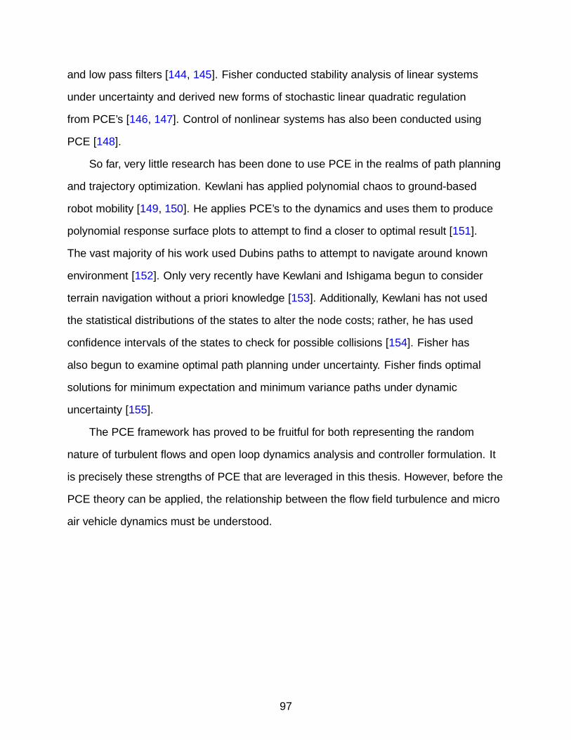
and low pass filters [144, 145]. Fisher conducted stability analysis of linear systems
under uncertainty and derived new forms of stochastic linear quadratic regulation
from PCE’s [146, 147]. Control of nonlinear systems has also been conducted using
PCE [148].
So far, very little research has been done to use PCE in the realms of path planning
and trajectory optimization. Kewlani has applied polynomial chaos to ground-based
robot mobility [149, 150]. He applies PCE’s to the dynamics and uses them to produce
polynomial response surface plots to attempt to find a closer to optimal result [151].
The vast majority of his work used Dubins paths to attempt to navigate around known
environment [152]. Only very recently have Kewlani and Ishigama begun to consider
terrain navigation without a priori knowledge [153]. Additionally, Kewlani has not used
the statistical distributions of the states to alter the node costs; rather, he has used
confidence intervals of the states to check for possible collisions [154]. Fisher has
also begun to examine optimal path planning under uncertainty. Fisher finds optimal
solutions for minimum expectation and minimum variance paths under dynamic
uncertainty [155].
The PCE framework has proved to be fruitful for both representing the random
nature of turbulent flows and open loop dynamics analysis and controller formulation. It
is precisely these strengths of PCE that are leveraged in this thesis. However, before the
PCE theory can be applied, the relationship between the flow field turbulence and micro
air vehicle dynamics must be understood.
97

CHAPTER 6AIRCRAFT MODEL PARAMETRIC IN TURBULENCE
A longitudinal flight dynamics model is derived that is parameterized in terms of
the turbulence intensity in order to analyze the effects of turbulence intensity on the
motion of an aircraft. The modes of this system are analyzed to find notable effects as
turbulence intensity increases.
6.1 Parameterized Model Derivation
The lift, drag, and pitching moment coefficients are expressed in terms of the
relevant terms found in the sweep model of the dynamic wind tunnel testing of
Section 4.2 and an additional term for the effect of the elevator is added. This term
for the effect of the elevator on the forces and moments arises out of a Taylor series
expansion. These expressions are shown in Equations 6–1 - 6–3.
CL =CLo + CLαα+ CLΛLEΛLE + CLαα+ CLθ θ + CLI I + CLα−ΛLEαΛLE + CLα−α
αα (6–1)
+ CLα−θαθ + CLα−θ
αθ + CLI2I 2 + CLδe δe
CD =CDo + CDαα+ CDΛLE
ΛLE + CDαα+ CDθ
θ + CDI I + CDα−ααα+ CDα−θ
αθ (6–2)
+ CDα−θαθ + CD
α2α2 + CD2
ΛLE
Λ2LE + CDδeδe
CM =CMo + CMαα+ CMΛLE
ΛLE + CMαα+ CMθ
θ + CMI I + CMα−ααα+ CMα−θ
αθ (6–3)
+ CMα−θαθ + CMδe
δe
A model is derived assuming an aircraft with no wing sweep, so those terms
including wing sweep are eliminated. Also, Equations 3–38 - 3–40 demonstrate that
θ = q when φ = 0. Thus, all θ terms will be replaced with q, due to the fact that
a longitudinal model is being constructed that assumes no nonzero values in the
lateral-directional states. Using this information, Equations 6–1 - 6–3 are rewritten,
replacing states with the perturbation equations shown in Equations 3–53 and 3–54.
The resulting equations are given in Equations 6–4 - 6–6.
98

CL =(CLo + CLααo + CLδe δeo + CLI I + CLI2 I2) + CLα∆α (6–4)
+ (CLq + CLα−qαo)∆q + (CLα + CLα−α
αo)∆α+ CLδe∆δe
CD =(CDo + CDααo + CD
α2α2o + CDδe
δeo + CDI I )
+ (CDα+ 2CD
α2αo)∆α+ (CDq + CDα−q
αo)∆q (6–5)
+ (CDα+ CDα−α
αo)∆α+ CDelev∆δe
CM =(CMo + CMααo + CMδe
δeo + CMI I ) + CMα∆α (6–6)
+ (CMq + CMα−qαo)∆q + (CMα
+ CMα−ααo)∆α+ CMδe
∆δe
The terms in Equations 6–4 - 6–6 that are not multiplied by state perturbations are
redefined in Equations 6–7 - 6–9.
CLtrim = CLo + CLααo + CLδe δeo + CLI I + CLI2 I2 (6–7)
CDtrim = CDo + CDααo + CD
α2α2o + CDδe
δeo + CDI I (6–8)
CMtrim = CMo + CMααo + CMδe
δeo + CMI I (6–9)
The lift, drag, and aerodynamic pitching moment are related to their respective
coefficients by Equations 6–10 - 6–12.
L = CL1
2ρV 2Sref (6–10)
D = CD1
2ρV 2Sref (6–11)
MAero = CM1
2ρV 2Sref cref (6–12)
Note that the dynamic pressure is inherent in each of Equations 6–10 - 6–12. The
dynamic pressure,Q, is defined in Equation 6–13.
99

Q =1
2ρV 2 (6–13)
The aircraft velocity component of Equations 6–10 - 6–12, V 2, can be rewritten as in
Equation 6–14 using the orthogonal velocity components of Equation 3–17.
V 2 = u2 + v 2 + w2 (6–14)
Now Equations 3–53 and 3–54 are substituted into Equation 6–14, resulting in
Equation 6–15.
V 2 =(uo +∆u)2 + (vo +∆v)
2 + (wo +∆w)2
=(u2o + w2o ) + 2uo∆u + 2wo∆w
=V 2∞ + 2uo∆u + 2wo∆w (6–15)
where V∞ =√
u2o + v2o + w
2o
Equations 6–4 - 6–9 and 6–15 are substituted into Equations 6–10 - 6–12. The
resulting equations are shown in Equations 6–16 - 6–18.
L =QSrefCLtrim + ρuoSrefCLtrim∆u + ρwoSrefCLtrim∆w +QSrefCLα∆α (6–16)
+QSref (CLq + CLα−qαo)∆q +QSref (CLα + CLα−α
αo)∆α+QSrefCLelev∆δe
D =QSrefCDtrim + ρuoSrefCDtrim∆u + ρwoSrefCDtrim∆w
+QSref (CDα+ 2CD
α2αo)∆α+QSref (CDq + CDα−q
αo)∆q (6–17)
+QSref (CDα+ CDα−α
αo)∆α+QSrefCDelev∆δe
MAero =QSref cref CMtrim + ρuoSref crefCMtrim∆u + ρwoSref cref CMtrim∆w
+QSref cref CMα∆α+QSref cref (CMq + CMα−q
αo)∆q (6–18)
+QSref cref (CMα+ CMα−α
αo)∆α+QSref cref CMelev∆δe
100

The perturbation terms in Equations 3–53 and 3–54 are substituted into the
longitudinal dynamics in Equation 3–52, resulting in Equations 6–19 - 6–21.
m∆u +mwo∆q =L(sinαo + cosαo∆α)− D(cosαo − sinαo∆α) (6–19)
−mg(sin θo + cos θo∆θ) + FThrustx
m∆w −muo∆q =− L(cosαo − sinαo∆α)− D(sinαo − cosαo∆α) (6–20)
+mg(cos θo − sin θo∆θ) + FThrustz
Iy∆q =MAero +MThrust (6–21)
Equations 6–16 - 6–18 are substituted into Equations 6–19 - 6–21. Terms are
collected, resulting in two sets of equations. The first set establish the requirements for
trimmed flight and are shown in Equations 6–22 - 6–24.
0 = QSrefCLtrim sinαo −QSrefCDtrim cosαo −mg sin θo + FThrustx (6–22)
0 = −QSref CLtrim cosαo −QSrefCDtrim sinαo +mg cos θo + FThrustz (6–23)
0 = MThrust +QSref cref CMtrim (6–24)
The second set of equations show the linearized perturbation dynamics of the
aircraft in Equations 6–25 - 6–27.
101

m∆u =ρuoSref (CLtrim sinαo − CDtrim cosαo)∆u + ρwoSref (CLtrim sinαo − CDtrim cosαo)∆w
+QSref[
sinαo(CLα + CDtrim) + cosαo(CLtrim − CDα− CD
α2αo)]
∆α (6–25)
+(
−mwo +QSref[
sinαo(CLq + CLα−qαo)− cosαo(CDq + CDα−q
αo)]
)
∆q
−mg cos θo∆θ +QSref (CLelev sinαo − CDelev cosαo)∆δe
+QSref[
sinαo(CLα + CLα−ααo)− cosαo(CDα
+ CDα−ααo)]
∆α
m∆w =− ρuoSref (CLtrim cosαo + CDtrim sinαo)∆u − ρwoSref (CLtrim cosαo + CDtrim sinαo)∆w
+QSref[
cosαo(CDtrim − CLα) + sinαo(CLtrim − CDα− 2CD
α2αo)]
∆α (6–26)
+(
muo −QSref[
cosαo(CLq + CLα−qαo) + sinαo(CDq + CDα−q
αo)]
)
∆q
−mg sin θo∆θ −QSref (CLelev cosαo + CDelev sinαo)∆δe
−QSref[
cosαo(CLα + CLα−ααo) + sinαo(CDα
+ CDα−ααo)]
∆α
Iy∆q =ρuoSref cref CMtrim∆u + ρwoSref crefCMtrim∆w +QSref cref CMα∆α
+QSref cref (CMq + CMα−q)∆q +QSref crefCMelev∆δe (6–27)
+QSref cref (CMα+ CMα−α
)∆α
Note from Chapter 3 that the angle of attack, α, is related to the vertical wind
velocity, w , through the relationship shown in Equation 6–28, and is also related to the
longitudinal wind velocity, u, through the relationship shown in Equation 6–29.
w =V∞ sinα (6–28)
u =V∞ cosα (6–29)
This relationship can be used to produce the mathematical relationships between
∆α and ∆w , and ∆α and ∆w , respectively. These relationships are shown in Equations 6–30
102

and 6–31, after substituting in the perturbation relationships of Equation 3–53 and
making small angle assumptions
∆w = −wo + V∞ sin(αo +∆α)
= −wo + V∞(sinαo cos∆α+ cosαo sin∆α)
= −wo + V∞ sinαo + V∞ cosαo∆α
= uo∆α (6–30)
d
dtw =
d
dt(V∞ sinα)
d
dt(wo +∆w) = V∞
d
dtsin(αo +∆α)
∆w = V∞ cos(αo +∆α)∆α
= V∞(cosαo cos∆α− sinαo sin∆α)∆α
= V∞ cosαo∆α − V∞ sinαo∆α∆α
= uo∆α (6–31)
Equations 6–30 and 6–31 are substituted into Equation 6–26 to produce the final
state space equation for the vertical velocity dynamics, shown in Equation 6–32.
103

∆w =1
m + QSrefuo
[
cosαo(CLα + CLα−ααo) + sinαo(CDα
+ CDα−ααo)]×
[
− ρuoSref
(
CLtrim cosαo + CDtrim sinαo
)
∆u
+
(
QSref
uo
[
cosαo(CDtrim − CLα) + sinαo(CLtrim − CDα− 2CD
α2αo)]
− ρwoSref
[
CLtrim cosαo + CDtrim sinαo
]
)
∆w (6–32)
+
(
muo −QSref[
cosαo(CLq + CLα−qαo) + sinαo(CDq + CDα−q
αo)]
)
∆q
−mg sin θo∆θ −QSref
(
CLelev cosαo + CDelev sinαo
)
∆δe
]
The remaining longitudinal dynamics equations, Equations 6–33 and 6–34 are
created by substituting Equations 6–30 - 6–32 into Equations 6–25 and 6–27.
104

∆u =ρuoSref
(
CLtrim sinαo − CDtrim cosαo
−
[
sinαo(CLα + CLα−ααo)− cosαo(CDα
+ CDα−ααo)][
CLtrim cosαo + CDtrim sinαo]
muoQSref
+ cosαo[
CLα + CLα−ααo]
+ sinαo[
CDα+ CDα−α
αo]
)
∆u
+
[
ρwoSref
(
CLtrim sinαo − CDtrim cosαo
−
[
sinαo(CLα + CLα−ααo)− cosαo(CDα
+ CDα−ααo)][
CLtrim cosαo + CDtrim sinαo]
muoQSref
+ cosαo[
CLα + CLα−ααo]
+ sinαo[
CDα+ CDα−α
αo]
)
+QSref
uo
(
sinαo[
CLα + CDtrim]
+ cosαo[
CLtrim − CDα− CD
α2αo]
+
[
sinαo(CLα + CLα−ααo)− cosαo(CDα
+ CDα−ααo)]
muoQSref
+ cosαo[
CLα + CLα−ααo]
+ sinαo[
CDα+ CDα−α
αo]×
[
cosαo(CDtrim − CLα) + sinαo(CLtrim − CDα− 2CD
α2)]
muoQSref
+ cosαo[
CLα + CLα−ααo]
+ sinαo[
CDα+ CDα−α
αo]
)
]
∆w (6–33)
+
(
−mwo +QSref
[
sinαo
(
CLq + CLα−qαo
)
− cosαo(
CDq + CDα−qαo
)
+
[
sinαo(
CLα + CLα−ααo)
− cosαo(
CDα+ CDα−α
αo)
]
muo +QSref
[
cosαo(
CLα + CLα−ααo)
+ sinαo(
CDα+ CDα−α
αo)
]×
[
muo −QSref(
cosαo [CLq + CLα−qαo ] + sinαo [CDq + CDα−q
αo ])
]
muo +QSref
[
cosαo(
CLα + CLα−ααo)
+ sinαo(
CDα+ CDα−α
αo)
]
]
)
∆q
−mg(
cos θo +sin θo
[
sinαo(CLα + CLα−ααo)− cosαo(CDα
+ CDα−α)]
muoQSref
+ cosαo[
CLα + CLα−ααo]
+ sinαo[
CDα+ CDα−α
αo]
)
∆θ
+QSref
(
CLelev sinαo − CDelev cosαo
−
[
sinαo(CLα + CLα−ααo)− cosαo(CDα
+ CDα−ααo)][
CLelev cosαo + CDelev sinαo]
muoQSref
+ cosαo[
CLα + CLα−ααo]
+ sinαo[
CDα+ CDα−α
αo]
)
∆δe
105

∆q =ρuoSref crefIy
(
CMtrim
−QSref
uo
[
CMα+ CMα−α
αo] CLtrim cosαo + CDtrim sinαo
m + QSrefuo
[
cosαo(CLα + CLα−ααo) + sinαo(CDα
+ CDα−ααo)]
)
∆u
+(
ρwoSref crefCMtrim +QSref cref
uoCMα
+QS2ref cref
uo
[
CMα+ CMα−α
αo]
×
Qu2o
[
cosαo(CDtrim − CLα) + sinαo(CLtrim − CDα− 2CD
α2αo)]
− ρwo[
CLtrim cosαo + CDtrim sinαo]
m + QSrefuo
[
cosαo(CLα + CLα−ααo) + sinαo(CDα
+ CDα−ααo)]
)
∆w
(6–34)
+QSref cref
Iy
(
CMq + CMα−qαo +
QSref
uo
[
CMα+ CMα−α
αo]
×
muoQSref
− cosαo(CLq + CLα−qαo)− sinαo(CDq + CDα−q
αo)
m + QSrefuo
[
cosαo(CLα + CLα−ααo) + sinαo(CDα
+ CDα−ααo)]
)
∆q
−QSref cref
uo Iy
[
CMα+ CMα−α
αo] mg sin θo
m + QSrefuo
[
cosαo(CLα + CLα−ααo) + sinαo(CDα
+ CDα−ααo)]∆θ
+QSref cref
Iy
(
CMelev
−QSref
uo
[
CMα+ CMα−α
αo] CLelev cosαo + CDelev sinαo
m + QSrefuo
[
cosαo(CLα + CLα−ααo) + sinαo(CDα
+ CDα−ααo)]
)
∆δe
6.2 Parameterized GenMAV Model
Equations 6–32 - 6–34 in conjunction with the continued use of ∆θ = q produce
a semi-complete four state linear model for the longitudinal dynamics of a micro air
vehicle in turbulence. Unfortunately this model is incomplete because the experimental
data was taken with the purpose of examining wing design parameters as a method to
mitigate the effects of turbulence, rather than to construct a complete dynamic model
of the aircraft. As a result, the data is missing some information needed to construct a
complete model of the longitudinal dynamics of the GenMAV.
So, the program files used to do a computer analysis of the aerodynamics of the
GenMAV are obtained and analyzed using the Athena Vortex Lattice (AVL) program
under flight conditions (angle of attack, velocity, Reynolds number, etc.) similar to those
106

used in the wind tunnel testing. AVL is a vortex-lattice based aerodynamic prediction
code that estimates the aerodynamics of both wings and slender bodies, such as the
fuselage [156]. This low-order code makes assumptions that the flow is incompressible
and inviscid; however, it is widely used in the community and is particularly accurate for
analyzing micro air vehicles with thin wings [27, 157–164].
AVL computes the open loop aircraft dynamics to fit the model shown in Equation 6–35.
For simplicity, the ∆ will be dropped from all ∆· terms from now on. It should be
assumed that all states in dynamic equations refer to perturbations about a trim
condition.
u
w
q
θ
=
A(1, 1) A(1, 2) A(1, 3) −9.81
A(2, 1) A(2, 2) A(2, 3) 0
A(3, 1) A(3, 2) A(3, 3) 0
0 0 1 0
u
w
q
θ
+
B(1, 1)
B(2, 1)
B(3, 1)
0
δe (6–35)
The resulting model from AVL is shown in Equation 6–36.
u
w
q
θ
=
−0.0232 0.9007 −2.515 −9.81
−1.0483 −2.9010 12.31 0
0.7266 −17.93 −6.222 0
0 0 1 0
u
w
q
θ
+
−0.0105
0.1302
3.798
0
δe (6–36)
At this point, there is a complete numerical model from Equation 6–36 that has no
parameterization with respect to turbulence, and an incomplete experimental model
from Section 6.1 that includes turbulence intensity as a model parameter. To combine
the information from the experimental and numerical models, the theoretical definition
of the linear aircraft dynamics is derived, including turbulence intensity as a parameter.
This theoretical definition should match the linear dynamics matrix that AVL has yielded,
when turbulence intensity is set to zero. So, the flight derivatives in the theoretical
107

definition of the linear dynamics matrix are set to values that would produce the AVL
system matrix for a turbulence intensity of zero. Then, the ratios between the computed
flight derivatives and the experimental flight derivatives are found and the coefficient
that multiplies the effect of the turbulence intensity parameter is scaled according to that
ratio.
For example, the element of the standard aircraft longitudinal dynamics matrix
in the second row and second column relates the force in the vertical direction to the
vertical velocity component experienced by the aircraft. If a cross coupling term between
w and I had been found, that element could be derived to be defined according to
Equation 6–37.
A(2, 2) = k ∗ (CZw + CZwI ∗ I + CZwI2 ∗ I2) (6–37)
where, k ∈ R is a product of physical constants
Then the value for A(2, 2) given by AVL is substituted into the left hand side of
Equation 6–37 and the turbulence intensity is set to zero. Thus, CZw is computed and
compared to the CZw found by wind tunnel testing. If the CZw from the AVL derivation is
half the size of the CZw found by wind tunnel testing, then the CZwI and CZwI2
found by
wind tunnel testing are also scaled by one-half. Thus, the relative effect of turbulence
intensity is maintained. The parameterized equation for A(2, 2) is now used.
In this way the effects of the turbulence intensity have been scaled to match the
force coefficients found by the numerical program and included in the system dynamics.
The result is a linear model of the longitudinal dynamics of the GenMAV that has been
parameterized with respect to turbulence intensity and matches the model produced by
a computational fluid dynamics code when the turbulence is set to zero.
The resulting model is shown in Equation 6–38.
108

u
w
q
θ
=
−0.0232 − 0.00608I + 0.00135I 2 0.901 + 0.193I − 0.0434I 2 −2.52 −9.81
−1.05− 0.2249I + 0.0506I 2 −2.90 − 0.444I + 0.0985I 2 12.3 0
0.727− 0.0357I + 0.000345I 2 −17.9 + 0.568I − 0.00270I 2 −6.22 0
0 0 1 0
u
w
q
θ
+
−0.0105
0.1302
3.7980
0
δe (6–38)
6.3 Modal Analysis of Parameterized System
An initial modal analysis is conducted on the parametrized aircraft dynamics
to evaluate the effects that a change in turbulence intensity has on the GenMAV’s
longitudinal modes.
6.3.1 Eigenvalue Analysis
The eigenvalues of the parametric system are plotted in Figure 6-1 as turbulence
intensity varies from 0% to 10%.
−6 −4 −2 0 2−15
−10
−5
0
5
10
15
Real Axis
Imag
inar
y A
xis
−1.5 −1 −0.5 0 0.5 1 1.5
−1
−0.5
0
0.5
1
Real Axis
Imag
inar
y A
xis
Figure 6-1. Eigenvalues of parameterized system (all eigenvalues shown on left,zoomed in on phugoid eigenvalues on right)
109

The left hand side of Figure 6-1 shows that the short period mode eigenvalues
begin to the left before moving back to the right as turbulence intensity increases. Thus,
the damping ratio increases slightly for small levels of turbulence but decreases much
more dramatically as turbulence levels get larger. Meanwhile, the short period mode
eigenvalues consistently move closer to the real axis, indicating that the frequency of
short period oscillations gets slightly smaller as turbulence levels increases.
When examining the phugoid eigenvalues alone in the right hand side of Figure 6-1,
it becomes clear that the changes in the phugoid eigenvalues are larger proportional
to the original eigenvalue; thus, the effect on the modal characteristics will be greater.
Figure 6-1 even shows that with high enough turbulence intensity (7.4% according to
this model), the oscillatory phugoid mode would break down into one convergent mode
and one divergent mode. This movement in the poles of the phugoid mode suggests
that for small levels of turbulence, the phugoid mode damping ratio and frequency would
increase, but as turbulence intensity continues to increase, both damping ratio and
frequency would decrease until it breaks into two real modes, one stable and the other
unstable. These trends are shown clearly in Figure 6-2. This finding should be tested
further to make any firm conclusions, because the wind tunnel testing upon which this
model is based only tested turbulence intensities up to 4%.
6.3.2 Mode Shape Analysis
Not only do the poles of the longitudinal system change as turbulence intensity
increases, but the shape of the modes change as well. The magnitude and phase of the
states relative to the pitch angle, θ, in each mode are shown in the following figures.
The relative magnitude and phase of the states in the short period mode are shown
in Figure 6-3.
Figure 6-3 shows that the shape of the short period mode under turbulence remains
similar to the shape of the mode in the absence of turbulence. The pitch rate dominates
while leading the pitch angle oscillations by just over 90o . The angle of attack varies by
110

0 2 4 6 8 10
−1
−0.5
0
0.5
1
Turbulence Intensity (%)
Dam
ping
Rat
io
0 2 4 6 8 100
2
4
6
8
10
12
14
16
Turbulence Intensity (%)
Fre
quen
cy (
rad/
s)
Figure 6-2. Frequency and damping of modes of the parameterized system (short period- dashed, phugoid that becomes unstable - solid, phugoid that becomesstable - dash-dot)
0 2 4 6 8 100
2
4
6
8
10
12
14
16
Turbulence Intensity (%)
Rel
ativ
e M
agni
tude
0 2 4 6 8 10
0
50
100
150
200
Turbulence Intensity (%)
Rel
ativ
e P
hase
(de
g)
Figure 6-3. Relative magnitude and phase of states in short period mode ofparameterized system (u component - solid, α component - dashed, qcomponent - dash-dot)
nearly exactly the same amount as the pitch angle and stays nearly in phase with the
pitch angle. The longitudinal velocity stays at nearly the exact same magnitude until the
turbulence begins to get very large, and shows some movement to be closer to being in
phase with the pitch angle. However, the longitudinal velocity component still remains
closer to being 180o out of phase until the turbulence intensity gets quite large.
The relative magnitude and phase of the states in the phugoid mode that becomes
an divergent mode are shown in Figure 6-4.
111

0 2 4 6 8 10−10
0
10
20
30
40
50
60
70
80
Turbulence Intensity (%)
Rel
ativ
e M
agni
tude
0 2 4 6 8 10
0
50
100
150
200
Turbulence Intensity (%)
Rel
ativ
e P
hase
(de
g)
Figure 6-4. Relative magnitude and phase of states in phugoid mode that becomes andivergent mode of the parameterized system (u component - solid, αcomponent - dashed, q component - dash-dot)
Figure 6-4 shows that until the phugoid mode disappears and becomes two
exponential modes, the shape of the mode stays largely constant. Under small
variations in turbulence intensity, the relative magnitudes of all components remain
roughly the same, with variations in longitudinal velocity dominating, while pitch angle
and pitch rate stay roughly of the same magnitude, and angle of attack variations
are minimal. Additionally, both pitch rate and longitudinal variations lead pitch angle
oscillations by about 90o while turbulence intensity variations remain small. The only
significant variation in the mode shape of the phugoid mode under small turbulence
levels is the phase by which the angle of attack leads the pitch rate. However, as
previously mentioned, the relative magnitude of the angle of attack is very small, so
this change in relative phase would not significantly alter the aircraft’s motion when this
mode is excited. When turbulence intensity becomes sufficiently large, the fluctuations in
the longitudinal velocity come to dominate to an even greater degree.
When the turbulence intensity becomes large enough as to eliminate the phugoid
mode, the resulting divergent mode demonstrates the same relative magnitudes
amongst the states as the phugoid mode. However, the longitudinal velocity and angle of
attack components vary in the opposite direction as the pitch angle and pitch rate.
112

The relative magnitude and phase of the states in the phugoid mode that becomes
a convergent mode are shown in Figure 6-5.
0 2 4 6 8 10−10
0
10
20
30
40
50
60
70
80
Turbulence Intensity (%)
Rel
ativ
e M
agni
tude
0 2 4 6 8 10
0
50
100
150
200
Turbulence Intensity (%)
Rel
ativ
e P
hase
(de
g)Figure 6-5. Relative magnitude and phase of states in phugoid mode that becomes a
convergent mode of the parameterized system (u component - solid, αcomponent - dashed, q component - dash-dot)
Figure 6-5 yields the same information on the phugoid mode as Figure 6-4.
However, the convergent mode that results from reaching sufficiently high turbulence
levels demonstrates pitch rate variations of opposite sign from those of the longitudinal
velocity, angle of attack, and pitch angle.
6.4 Linearized Model
The model derived from the wind tunnel data and shown in Equation 6–38 has
components of the force and moment derivatives that are quadratic with respect to
turbulence intensity. Such a model is difficult to analyze using the polynomial chaos
methods upon which the remainder of research is based. As a result, this model is made
linear with respect to turbulence intensity and demonstrated to be a good approximation
of the originally derived model.
6.4.1 Linearization of Model with Respect to Turbulence
To linearize the model, a turbulence intensity of 3.5% is chosen to be the nominal
condition about which the force and moment derivatives are linearized. This value is
chosen because when used in conjunction with a standard deviation of 1% turbulence to
113

be used in later analysis, the resulting range of turbulence levels is mostly contained
within the tested range of turbulence levels from Chapter 4 and avoids negative
turbulence intensity levels, which would violate mathematical laws. Additionally, this
level of turbulence intensity lies in the middle of the range over which the linearized
model can be trusted, 0-7%.
So, turbulence intensity is given the form previously seen in perturbation dynamics
and shown in Equation 6–39.
I = 3.5 + I (6–39)
Equation 6–39 is substituted into the parametric model from Equation 6–38 and
I 2 terms are ignored. The resulting system is not only linear in that its form can be
expressed in vector and matrix format, but now the force and moment derivatives
are linear with respect to turbulence intensity. This linearized system is shown in
Equation 6–40.
u
w
q
θ
=
−0.02798 + 0.003352I 1.045− 0.1107I −2.515 −9.81
−1.216 + 0.1292I −3.250 + 0.2448I 12.31 0
0.6060 − 0.03324I −15.97 + 0.5494I −6.222 0
0 0 1 0
u
w
q
θ
+
−0.0105
0.1302
13.7980
0
δe (6–40)
The linearized model of Equation 6–40 needs to be compared to the quadratic
parametric model of Equation 6–38 to ensure that they demonstrate similar effects
with respect to variations in turbulence intensity. Comparisons are made between the
114

eigenvalues and the mode shapes of the modes of each of these systems to show the
range through which the linearized model agrees with the quadratic model.
6.4.2 Eigenvalue Analysis
The eigenvalues of the linearized parametric system are plotted in Figure 6-6 as
turbulence intensity varies from 0% to 10%.
−6 −4 −2 0 2−15
−10
−5
0
5
10
15
Real Axis
Imag
inar
y A
xis
−1.5 −1 −0.5 0 0.5 1 1.5
−1
−0.5
0
0.5
1
Real Axis
Imag
inar
y A
xis
Figure 6-6. Eigenvalues of linearized parametric system (all eigenvalues shown on left,zoomed in on phugoid eigenvalues on right)
The eigenvalues of the linearized system, shown in Figure 6-6, follow similar trends
to those seen in the quadratic model, shown in Figure 6-1. However, the similarities
between the damping ratio and frequency of the longitudinal modes of the quadratic and
linear parametric systems are best shown in Figure 6-7.
It is apparent from Figure 6-7 that the linearized system is in agreement with the
quadratic system on the frequency and damping ratios of the longitudinal modes until
turbulence intensity exceeds 7% and the phugoid mode nears the point at which it splits
into two exponential modes.
6.4.3 Mode Shape Analysis
The relative magnitudes and phases of the longitudinal states in the short period
mode are shown in Figure 6-8. Just as in Subsection 6.3.2, all magnitudes and phases
are made relative to the θ state.
115
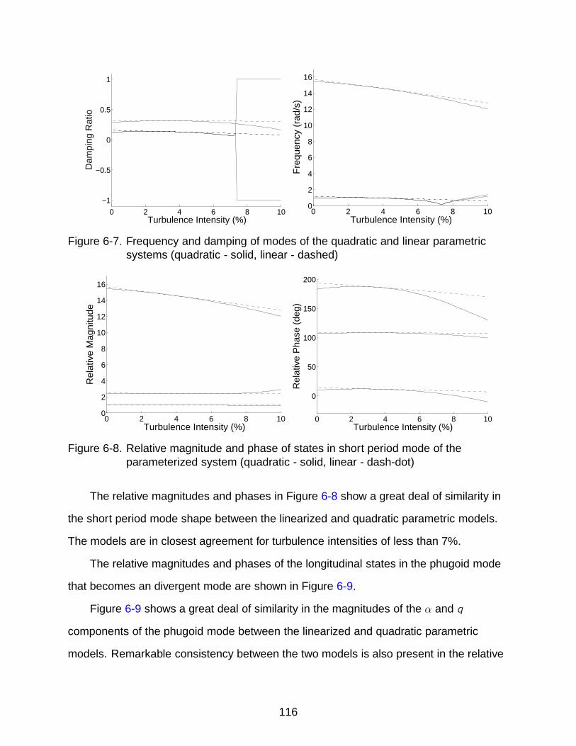
0 2 4 6 8 10
−1
−0.5
0
0.5
1
Turbulence Intensity (%)
Dam
ping
Rat
io
0 2 4 6 8 100
2
4
6
8
10
12
14
16
Turbulence Intensity (%)
Fre
quen
cy (
rad/
s)
Figure 6-7. Frequency and damping of modes of the quadratic and linear parametricsystems (quadratic - solid, linear - dashed)
0 2 4 6 8 100
2
4
6
8
10
12
14
16
Turbulence Intensity (%)
Rel
ativ
e M
agni
tude
0 2 4 6 8 10
0
50
100
150
200
Turbulence Intensity (%)
Rel
ativ
e P
hase
(de
g)
Figure 6-8. Relative magnitude and phase of states in short period mode of theparameterized system (quadratic - solid, linear - dash-dot)
The relative magnitudes and phases in Figure 6-8 show a great deal of similarity in
the short period mode shape between the linearized and quadratic parametric models.
The models are in closest agreement for turbulence intensities of less than 7%.
The relative magnitudes and phases of the longitudinal states in the phugoid mode
that becomes an divergent mode are shown in Figure 6-9.
Figure 6-9 shows a great deal of similarity in the magnitudes of the α and q
components of the phugoid mode between the linearized and quadratic parametric
models. Remarkable consistency between the two models is also present in the relative
116

0 2 4 6 8 10−10
0
10
20
30
40
50
60
70
80
Turbulence Intensity (%)
Rel
ativ
e M
agni
tude
0 2 4 6 8 10
0
50
100
150
200
Turbulence Intensity (%)
Rel
ativ
e P
hase
(de
g)
Figure 6-9. Relative magnitude and phase of states in phugoid mode that becomes andivergent mode of the parameterized system (quadratic - solid, linear -dash-dot)
phases of the q and u components. The significant differences between the two models
manifest themselves in the relative magnitude of the u component and the relative phase
of the α component. Just as in Subsection 6.3.2, differences in the relative phase of
the angle of attack can be ignored because the magnitude of variations in the angle
of attack is so small in the phugoid mode. The differences in the magnitude of the
variations of longitudinal velocity grow large when the phugoid mode of the quadratic
system nears the point at which it splits into two exponential modes. So, within the range
of 0-7% turbulence, the linearized system approximates the changes seen in the modes
of the quadratic system.
The relative magnitudes and phases of the longitudinal states in the phugoid mode
that becomes a convergent mode are shown in Figure 6-10.
Figure 6-10 yields the same insight that came from Figure 6-9.
6.5 Polynomial Chaos Model
Now that the linearized parametric model has been verified, this variation in
dynamics can be approximated using the polynomial chaos theory detailed in Chapter 5.
117

0 2 4 6 8 10−10
0
10
20
30
40
50
60
70
80
Turbulence Intensity (%)
Rel
ativ
e M
agni
tude
0 2 4 6 8 10
0
50
100
150
200
Turbulence Intensity (%)
Rel
ativ
e P
hase
(de
g)
Figure 6-10. Relative magnitude and phase of states in phugoid mode that becomes aconvergent mode of the parameterized system (quadratic - solid, linear -dash-dot)
6.5.1 Order of PC Approximation
Before the modes of the PC system can be analyzed, some verification must be
done to ensure that the PC system is implemented correctly. Recall from Subsection 5.4.1
that convergence for higher order terms is not guaranteed.
So, the parametric dynamics of Equation 6–40 is expanded by the process shown
in Section 5.3 using Hermite polynomials up to the 9th order. As a result of this process,
the PCE system has 40 states and exhibits 20 oscillatory modes. Within each mode
the first 10 states relate to the u state, the second group of 10 states relate to the w
state, the third group of 10 states relate to the q state, and the final 10 states relate to
the θ state. The first term related to the u state is the 0th order term of the u state. The
magnitude of this term is average across all 10 modes. This process is repeated for the
following terms related to the u state and for all the terms related to the other physical
states. This process yields the relative magnitude of the modal components averaged
across all 20 modes. The result is shown in Figure 6-11.
Figure 6-11 shows that the average relative magnitude of the modal components
steadily declines with increasing order once the order passes four. This trend indicates
that there is much less variation in the higher order terms of the PCE system compared
118

0 2 4 6 8 100
0.05
0.1
0.15
0.2
0.25
0.3
0.35
Polynomial Order
Ave
rage
Rel
ativ
e M
agni
tude
Figure 6-11. Average relative magnitude of modal components when using ninth orderPC approximation
to the lower order terms; signifying that the PCE system has converged and is capturing
the much of the important statistical fluctuations in the physical states.
Additionally, it is noted from Figure 6-11 that higher order terms are much smaller
than the lower order terms. This feature indicates that there is little activity in the higher
order moments of the state variables, and that a lower order approximation could
be used to capture most of the information that PC offers. As a result, a fifth order
approximation is used for all later analysis. Figure 6-12 shows the average relative
magnitude of the modal components when using a fifth order PC approximation.
It is clear from Figure 6-12 that the higher order terms have sufficiently decreased in
magnitude to conclude that this approximation has also converged and can be expected
to capture most of the fluctuation in the moments of the states of the parametric system.
This fifth order PCE expansion is used for analysis of a PCE expanded system to reduce
the computation times and simplify analysis.
119

0 1 2 3 4 50
0.05
0.1
0.15
0.2
0.25
0.3
0.35
0.4
Polynomial Order
Ave
rage
Rel
ativ
e M
agni
tude
Figure 6-12. Average relative magnitude of modal components when using fifth orderPC approximation
6.5.2 Eigenvalue Analysis
The eigenvalues of the expanded system are plotted over the eigenvalues of the
parametric system in Figure 6-13.
−6 −4 −2 0 2−15
−10
−5
0
5
10
15
Real Axis
Imag
inar
y A
xis
−1.5 −1 −0.5 0 0.5 1 1.5
−1
−0.5
0
0.5
1
Real Axis
Imag
inar
y A
xis
Figure 6-13. Eigenvalues of PC expanded system (short period modes are shown onthe left, and the phugoid modes are shown on the right)
The eigenvalues of the expanded system can be separated into two groups that
cluster around the eigenvalues of the parametric system. As a result, the modes that
have eigenvalues near the short period eigenvalues will be referred to as short period
120

modes, and the same for the phugoid modes. The modes 1-6 are short period modes
and modes 7-12 are phugoid modes.
6.5.3 Mode Shape Analysis
The magnitude and phase of the eigenvectors also support the notion of grouping
the modes in such a way that compares them to the original physical modes.
The relative magnitude of the short period eigenvectors of the parameterized
system are normalized with respect to the state θ and shown in Table 6-1. This
information is also compared to the relative magnitude of 0th order stochastic states
(u0, w0, and q0) in Modes 1-6 of the expanded system in Table 6-1.
Parameterized System Expanded SystemState Short Period Mode Mode 1 Mode 2 Mode 3 Mode 4 Mode 5 Mode 6u 2.427 2.408 2.394 2.375 2.385 2.375 2.376α 0.9891 0.9864 0.9837 0.9755 0.9814 0.9788 0.9771q 14.71 14.33 13.95 12.86 13.66 13.37 13.08
Table 6-1. Magnitudes of state fluctuations relative to θ for short period modes
The relative phase of the short period eigenvectors of the parameterized system
are normalized with respect to the state θ and shown in Table 6-2. This information is
also compared to the relative phase of 0th order stochastic states in Modes 1-6 of the
expanded system in Table 6-2.
Parameterized System Expanded SystemState Short Period Mode Mode 1 Mode 2 Mode 3 Mode 4 Mode 5 Mode 6u 186.6o 183.6o 180.4o 170.9o 178.0o 175.4o 172.9o
α 11.79o 10.90o 10.00o 7.298o 9.296o 8.580o 7.857o
q 108.3o 108.2o 108.1o 107.8o 108.0o 108.0o 107.9o
Table 6-2. Phase lead of states relative to θ for short period modes
Tables 6-1 and 6-2 show that there is a great deal of similarity between the mode
shapes of the parameterized system and the 0th order states of the expanded system
in both the relative magnitudes and phases. From this information we could anticipate
that the expected short period response of the system in the presence of uncertainty
121

in turbulence intensity will be very similar to the response seen without uncertainty in
turbulence intensity.
The relative magnitude of the phugoid eigenvectors of the parameterized system
are normalized with respect to the state θ and shown in Table 6-3. This information
is also compared to the relative magnitude of 0th order stochastic states in Modes
7-12 of the expanded system in Table 6-3. Modes 8 and 10 do exhibit some significant
deviations in the relative magnitudes of the u and q states. However, the relative
magnitudes for all states are the same order of magnitude in all of the modes.
Parameterized System Expanded SystemState Phugoid Mode Mode 7 Mode 8 Mode 9 Mode 10 Mode 11 Mode 12u 9.921 10.63 15.82 11.46 14.24 12.16 13.00α 0.0042 0.0044 0.0164 0.0055 0.0122 0.0070 0.0090q 0.9846 0.9195 0.6187 0.8532 0.6872 0.8041 0.7524
Table 6-3. Magnitudes of state fluctuations relative to θ for phugoid modes
The relative phase of the phugoid eigenvectors of the parameterized system are
normalized with respect to the state θ and shown in Table 6-4. This information is
also compared to the relative phase of 0th order stochastic states in Modes 1-6 of the
expanded system in Table 6-4. The relative phase of the α state varies significantly
between the modes, but the magnitude of fluctuations in the α state, seen in Table 6-3,
are so small compared to those of the other states as to render the phase differences
inconsequential. The relative phases of the u and q states are remarkably similar
amongst the modes.
Parameterized System Expanded SystemState Phugoid Mode Mode 7 Mode 8 Mode 9 Mode 10 Mode 11 Mode 12u 98.49o 97.74o 94.39o 96.96o 95.09o 96.41o 95.85o
α 8.655o 33.34o 85.51o 55.63o 81.43o 67.12o 75.22o
q 97.68o 97.18o 95.00o 96.71o 95.53o 96.34o 95.95o
Table 6-4. Phase lead of states relative to θ for phugoid modes
122

Tables 6-3 and 6-4 show that there is a some similarity between the mode shapes
of the parameterized system and the 0th order states of the expanded system in both
the relative magnitudes and phases. From this information, we could anticipate that
the expected phugoid response of the aircraft in the presence of uncertainty in the
turbulence intensity will look similar to the response of the aircraft in the absence of
uncertainty. However, it is difficult to see from this information exactly how the response
in the presence of uncertainty will differ from the response in the absence of uncertainty.
6.5.4 Analysis of Short Period Modes
The standard aircraft short period mode is dominated by energy in the α, q, and
θ states, so it is expected that a simulation of one of the short period modes of the
expanded system will show most of its fluctuation in these states. Figure 6-14 shows the
mean time response of all four physical states when one of the six short period modes of
the expanded system is excited.
0 0.5 1 1.5−15
−10
−5
0
5
Time (s)
u (m/s)alpha (deg)q (deg/s)theta (deg)
Figure 6-14. Mean values of all 4 states for one short period mode
Figure 6-14 shows that the short period modes of expanded system are similar
to the short period mode of the parameterized system in the magnitude of the state
123

variations. The other five short period modes show similar trends to Figure 6-14. The
mean and variance bounds of all four physical states in all six short period modes of the
expanded system are shown in Figure 6-15.
0 0.5 1 1.5−0.5
0
0.5
Time (s)
u (m
/s)
MeanVariance Bounds
0 0.5 1 1.5
−10
−5
0
5
10
Time (s)al
pha
(deg
)
MeanVariance Bounds
0 0.5 1 1.5
−200
−100
0
100
200
Time (s)
q (d
eg/s
)
MeanVariance Bounds
0 0.5 1 1.5
−10
−5
0
5
10
Time (s)
thet
a (d
eg)
MeanVariance Bounds
Figure 6-15. Mean and variance bounds of longitudinal states for all 6 short periodmodes
All six of these modes in all three dominant states show a great deal of phase
similarity between the variance and mean. The variance reaches a minimum at the
same time as the mean crosses zero. So, it appears that even under uncertainty
in turbulence intensity, the physical states related to the short period mode can be
predicted with a great deal of precision at certain time intervals, specifically, the zero
crossings of each state.
124

6.5.5 Analysis of Phugoid Modes
The standard aircraft phugoid mode is dominated by energy in the u, q, and θ
states, so it is expected that a simulation of one of the phugoid modes of the expanded
system will show most of its fluctuation in these states. Figure 6-16 shows the variation
in the mean values of all four states for one of the six phugoid modes of the expanded
system.
0 10 20 30 40 50 60
−1
−0.5
0
0.5
1
1.5
Time (s)
u (m/s)alpha (deg)q (deg/s)theta (deg)
Figure 6-16. Mean values of states for one phugoid mode
Figure 6-16 shows that the phugoid modes of expanded system are similar to the
phugoid mode of the parameterized system in the magnitude of the state variations. The
other five phugoid modes show similar trends to Figure 6-16. The mean and variance
bounds of all physical states in all six of the phugoid modes of the expanded system are
shown in Figure 6-17.
It is once again noted is that the variance seems to reach a minimum whenever the
mean of the state crosses zero; however, the variance does not get as close to zero for
some modes as for others. This can be noted in Figure 6-17. That figure shows the time
evolution of the variance bounds on the pitch angle under all of the phugoid modes. If
125

0 10 20 30 40 50 60−6
−4
−2
0
2
4
6
Time (s)
u (m
/s)
MeanVariance Bounds
0 10 20 30 40 50 60
−0.2
−0.1
0
0.1
0.2
0.3
Time (s)
alph
a (d
eg)
MeanVariance Bounds
0 10 20 30 40 50 60
−20
−15
−10
−5
0
5
10
15
20
Time (s)
q (d
eg/s
)
MeanVariance Bounds
0 10 20 30 40 50 60−20
−15
−10
−5
0
5
10
15
20
Time (s)
thet
a (d
eg)
MeanVariance Bounds
Figure 6-17. Mean and variance bounds of longitudinal states for all 6 phugoid modes
Equations 5–26 and 5–27 are applied to the aircraft system, then the mean of the pitch
angle is the 19th state of the expanded system (from hereon this state is referred to as
θ0), and the variance of the pitch rate is the sum of the squares of the 20th through 24th
states of the system (from hereon these states are referred to as θ1 through θ5). Thus,
an analysis of the phase difference between these states of the expanded system yields
insight as to why the variance reaches a minimum, and in some cases seems to go to
zero at the same time as the mean. The phase of the states θ0 through θ5 for Modes 10
and 11 are shown in Table 6-5.
Table 6-5 shows that the reason the variance is a minimum when the mean crosses
zero is because all of the states related to the physical state θ are nearly in phase or
180o out of phase. Thus, they would all cross zero at the same time, causing a minimum
126

State Mode 10 Mode 11θ0 0 0θ1 -0.5o 183.6o
θ2 -3.4o 180.2o
θ3 180.3o 145.7o
θ4 179.7o -2.1o
θ5 177.3o 181.3o
Table 6-5. Phase lag of states of expanded system
in the variance of state θ. The reason that Mode 11 does not have the variance get as
small as in Mode 10 is because θ3 in Mode 11 is 145o out of phase with θ0, so it is large
enough to yield a significant variance when the mean of the state is zero.
6.5.6 Example Simulation
The modal analysis of the preceding sections has yielded some insight into the
modes of the open loop response of the GenMAV under uncertainty in the turbulence
intensity, but it is unclear how these modes interact with one another. To understand the
modal interactions, an example simulation is run with initial conditions that will excite all
of the modes of the system.
The data presented in the rest of this subsection all relate to a simulation of the
expanded system conducted using the initial conditions shown in Equation 6–41.
These initial conditions are a special case in that they represent an initial state with no
uncertainty; the initial physical states are known exactly and are equal to the 0th order
states in the expanded system.
127

u0 = 2 m/s
u1, ... , u5 = 0 m/s
w0 = 1 m/s
w1, ... ,w5 = 0 m/s (6–41)
q0 = −0.2 rad/s
q1, ... , q5 = 0 rad/s
θ0 = 0.1 rad
θ1, ... , θ5 = 0 rad
Figure ?? shows the time evolution of the mean and variance bounds of all four
states given the initial conditions of Equation 6–41.
The most interesting feature to note in Figure 6-18 is the growth and consequential
decay in state uncertainty. The magnitude of the uncertainty in the states is most
pronounced in the physical states u and θ. It is interesting to note that despite the fact
that for many of the modes of the expanded system, the variance decreased to nearly
zero when the mean states crossed zero; yet in this simulation, the state uncertainty
does not approach zero until sufficient time has passed to allow all the states of the
expanded system to decay to zero. This example demonstrates how the modes combine
in varying magnitudes and at varying relative phase angles to produce the time evolution
of the system state uncertainty.
Figure 6-18 shows the long term effects of uncertainty in turbulence intensity on
the longitudinal states of the GenMAV, but the short term effects are not clear from this
figure. So, Figure 6-19 shows the time evolution of the mean and variance bounds of all
four states given the same initial conditions, but only shows the time history of the first
few seconds. Note that the short period modal analysis of Subsection 6.5.4 showed a
128

0 20 40 60 80 100−3
−2
−1
0
1
2
3
Time (s)
u (m
/s)
0 20 40 60 80 100−2
−1
0
1
2
3
4
5
Time (s)
alph
a (d
eg)
0 20 40 60 80 100−40
−30
−20
−10
0
10
20
30
Time (s)
q (d
eg/s
)
0 20 40 60 80 100−10
−5
0
5
10
15
Time (s)
thet
a (d
eg)
Figure 6-18. Mean and variance bounds of all states for example simulation
settling time of around one second, so Figure 6-19 shows three seconds of the example
simulation to observe the transition from short period to phugoid dynamics.
The contrast in the time evolution of the state uncertainties between the different
states is remarkable. The angle of attack, α, shows almost no uncertainty, yet the
states u and θ show large uncertainty growth within the first second. The pitch rate, q,
is perhaps the most interesting state to observe, because its uncertainty begins to grow
before decaying to nearly zero, yet then begins to grow again.
These trends are likely explained by observations made previously that the phugoid
modes are more substantially affected by the uncertainty in the turbulence intensity. The
angle of attack, α, plays almost no role in the phugoid modes, and any uncertainty in α
due to the short period modes is minimal and decays quickly. The pitch rate, q, plays
129

0 1 2 3 4−2
−1
0
1
2
3
Time (s)
u (m
/s)
0 1 2 3 4−2
−1
0
1
2
3
4
5
Time (s)
alph
a (d
eg)
0 1 2 3 4−40
−30
−20
−10
0
10
20
30
Time (s)
q (d
eg/s
)
0 1 2 3 4−5
0
5
10
15
Time (s)
thet
a (d
eg)
Figure 6-19. Mean and variance bounds of all states for example simulation
a much more significant role in the short period modes, yet still has a presence in the
phugoid modes. So the uncertainty in q due to the short period modes is observed,
decays quickly, and then uncertainty due to the phugoid modes begins to grow as the
phugoid dynamics dominate the system. The states u and θ are large components of
the phugoid mode, so the uncertainty in the turbulence intensity propagates through the
phugoid modes of the expanded system and results in large growth in the uncertainty of
these states.
6.5.7 Effects of Uncertain Parameter Distribution
The results shown so far in Section 6.5 have assumed a Gaussian distribution for
the turbulence intensity with a mean of 3.5% turbulence and a standard deviation of 1%
turbulence. However, this distribution is not obtained from any scientific method; rather,
130

it is assumed using previous work on atmospheric turbulence as a guide. Therefore, it
would be interesting to find what effects would result from a change in the probability
density function of the atmospheric turbulence.
A new probability density function is assumed for turbulence intensity, with a mean
of 3.5% turbulence and a standard deviation of 2% turbulence. The same PCE process
as before is performed on the parameterized system using the new probability density
function for turbulence intensity. Figure 6-20 shows the eigenvalues of the expanded
system under two different distributions of uncertainty with respect to turbulence
intensity.
−4.5 −4 −3.5 −3−15
−10
−5
0
5
10
15
Real Axis
Imag
inar
y A
xis
Std Dev = 1Std Dev = 2
−0.6 −0.4 −0.2 0 0.2 0.4 0.6−1
−0.5
0
0.5
1
Real Axis
Imag
inar
y A
xis
Std Dev = 1Std Dev = 2
Figure 6-20. Eigenvalues of expanded system using two distributions of turbulenceintensity
It is apparent from Figure 6-20 that the eigenvalues of the short period modes
are relatively unaffected by the increase in variance of the turbulence intensity. Some
eigenvalues moved a small amount in the direction of the negative real axis under
the wider distribution, but the change relative to the location of the eigenvalues under
the tighter distribution is small. The eigenvalues of the phugoid mode moved quite
significantly in the presence of the wider distribution of turbulence intensity. The new
uncertain parameter distribution pushed one of the eigenvalue pairs to the real axis, thus
splitting it into a convergent and a divergent mode. This occurrence fits with Figure 6-1,
which suggested that if the turbulence intensity grows large enough, the phugoid
131

mode would be split into a convergent and a divergent mode. It appears that the wider
distribution of turbulence intensity has brought that effect into the expanded system.
The phugoid modes of the expanded system under the wider distribution are
now analyzed. The convergent and divergent modes will not be examined due to the
previously mentioned doubt as to the veracity of these modes. Figure 6-21 shows the
longitudinal states for the five stable phugoid modes present in the expanded system
under the wider distribution of turbulence intensity.
0 10 20 30 40 50 60−6
−4
−2
0
2
4
6
Time (s)
u (m
/s)
MeanVariance Bounds
0 10 20 30 40 50 60
−0.6
−0.4
−0.2
0
0.2
0.4
0.6
Time (s)
alph
a (d
eg)
MeanVariance Bounds
0 10 20 30 40 50 60−20
−15
−10
−5
0
5
10
15
20
Time (s)
q (d
eg/s
)
MeanVariance Bounds
0 10 20 30 40 50 60−20
−15
−10
−5
0
5
10
15
20
Time (s)
thet
a (d
eg)
MeanVariance Bounds
Figure 6-21. Mean and variance bounds of longitudinal states for all stable phugoidmodes, given a wider distribution of turbulence intensity
Figure 6-21 shows a similar mix of ratios of mean and variance response that
appeared in Figure 6-17. However, the phase differences between the modes have
become even more pronounced, and the frequencies at which they oscillate have
132

become even more varied. One of the phugoid modes of this expanded system shows a
very low frequency of oscillation and very low damping ratio in the variance of the states.
This data indicates that uncertainty with respect to turbulence intensity strongly affects
the phugoid mode and results in stronger uncertainty propagating through the phugoid
mode as the variance of turbulence intensity increases.
133

CHAPTER 7STOCHASTIC PATH EVALUATION METHODS
This chapter introduces techniques that can be used to apply polynomial chaos
(PC) theory to path evaluation strategies. The basic concept is to use the information
that PC analysis provides with the principles of conditional probability to derive the
probability of mission success with a defined vehicle, controller, environment, and
desired path. The techniques are explained in general in Section 7.2 such that they
can be applied to many definitions of mission success. The techniques are applicable
as long as mission success is defined as some mathematical combination of mission
states and time, such as obstacle avoidance, sensor coverage, or waypoint navigation.
Sections 7.3 and 7.4 show examples of the algorithm being applied to defined mission
success metrics.
7.1 Probability Background
Constructing the path evaluation algorithm requires some background information
into probability and set theory.
A probability space is defined using three parts: a sample space, a set of events,
and the corresponding probabilities of the events occurring. For this reason, a probability
space is said to be defined a probability “triple”, (Ω,F ,P). The sample space, Ω, is the
set of all possible outcomes.
The union of two sets A1 and A2 is defined in Equation 7–1.
A1 ∪ A2 = all elements contained in either A1 or A2 (7–1)
The intersection of two sets A1 and A2 is defined in Equation 7–2.
A1 ∩ A2 = all elements contained in both A1 and A2 (7–2)
The complement of set A is defined in Equation 7–3.
134

Ac = all elements in Ω not contained in A (7–3)
The relative complement of set A with respect to set B is defined in Equation 7–4.
A− B = all elements in A not contained in B (7–4)
Given a sample space Ω, a partition of Ω is defined in Equation 7–5.
partition of Ω is Ai : i ∈ I such that ∪i Ai = Ω (7–5)
where, Ai ∩ Aj = ∅ for i 6= j
An example of a sample space is shown in Figure 7-1.
Ω
A
B
C
Figure 7-1. Partition of an example sample space
A partition of this sample space could be written as shown in Equation 7–6.
Ω = A ∪ (B − C) ∪ (C − B) ∪ (B ∩ C) ∪ (A ∪ B ∪ C)c (7–6)
The probability of an event occurring is a norm function that can range in value from
0 to 1. For example, in Figure 7-1, the probability of event C occurring, P(C), would take
on a positive value somewhere between 0 and 1.
135

Probabilities can also be conditioned upon other events occurring. The probability of
event A1 occurring conditioned on event A2 occurring is defined by Equation 7–7.
P(A1 | A2) =P(A1 ∩ A2)
P(A2)(7–7)
For example, in Figure 7-1, the probability of event C occurring, P(C), would be
smaller than the probability of event C occurring conditioned on the fact that event B
had occurred, P(C | B). Additionally, it can be seen that the probability of event C
occurring conditioned on the fact that event A had occurred, P(C | A), would be equal to
0, because P(A ∩ C) is equal to 0.
Partitions and conditional probabilities can be used in concert through the law
of total probability. The law of conditional probability states that if Ai : i ∈ I forms
a partition of Ω, then the probability of event B occurring can be expressed as in
Equation 7–8.
P(B) =∑
i∈I
P(B ∩ Ai) (7–8)
Probability distribution functions (PDFs) are another method of expressing the
probability of an event occurring. If a random variable, ∆, can take one of any countable
number of real values, then the PDF of ∆, F∆, is defined in Equation 7–9.
F∆(x) = P(∆ = x) (7–9)
Thus, a PDF is a useful description of the probability of discrete events occurring.
Cumulative distribution functions (CDFs) provide similar information to PDFs although in
a slightly different form, and can be used for both discrete and continuous distributions.
A CDF, G∆, is defined according to Equation 7–10.
G∆(x) = P(∆ ≤ x) (7–10)
136

If a random variable has a CDF that is continuous and differentiable, then it
also possesses a probability density function (pdf). A pdf, f∆, is defined according to
Equation 7–11.
f∆(x) =∂G∆(x)
∂x(7–11)
Note that a pdf only exists if the random variable exhibits a CDF that is both
continuous differentiable, and that the existence of a pdf implies that the probability of
the random variable taking any singular value is negligible. Equation 7–12 demonstrates
this fact.
P(∆ = x) = 0 (7–12)
if ∃ f∆(x)
7.2 Stochastic State Generation Algorithm
The algorithm to generate stochastic state information that is amenable to path
evaluation consists of combining the PC expanded dynamics information, which is
explained in Chapter 6, with a partition of the sample space of the given mission.
For example, if the goal of a mission is to reach a final position (RFP) while passing
through one waypoint region (WP1), the partition of the sample space of this mission
would look like Figure 7-2.
The probability of mission success for this example would be found using Equation 7–13.
P(success) = P(RFP ∩WP1) (7–13)
= P(RFP |WP1)P(WP1)
137

Ω
Reach Final Position
(RFP)
Pass through
Waypoint 1
(WP1)
Figure 7-2. Partition of sample space of mission with one waypoint(hatched area indicates set of results with mission success)
If the environment in question has two waypoint regions (WP1 andWP2) and the
vehicle has a nonzero probability of passing through both, then the partition of the
sample space would look like Figure 7-3.
Ω
Reach Final Position
(RFP)
Pass through
Waypoint 1
(WP1)
Pass through
Waypoint 2
(WP2)
Figure 7-3. Partition of sample space of mission with two waypoints(hatched area indicates set of results with mission success)
The probability of mission success for this example would be found using Equation 7–14.
138

P(success) = P(RFP ∩WP2 ∩WP1)
= P(RFP |WP2 ∩WP1)P(WP2 ∩WP1) (7–14)
= P(RFP |WP2 ∩WP1)P(WP2 |WP1)P(WP1)
If the waypoint regions from the previous two examples are no-fly zones instead,
then mission success would be described as reaching the final position while avoiding
passing through any no-fly zone. If there is only one no-fly zone, then the resulting
partition would appear as shown in Figure 7-4.
Ω
Reach Final Position
(RFP)
Pass through
No- y Zone 1
(NF1)
Figure 7-4. Partition of sample space of mission with one no-fly zone(hatched area indicates set of results with mission success)
The probability of mission success with one no-fly zone (NF1) would be described
using Equation 7–15.
P(success) = P(RFP)− P(RFP ∩ NF1) (7–15)
= P(RFP)− P(RFP | NF1)P(NF1)
If there is only one no-fly zone, then the resulting partition would appear as shown
in Figure 7-5.
139

Ω
Reach Final Position
(RFP)
Pass through
No-y Zone 1
(NF1)
Pass through
No-y Zone 2
(NF2)
Figure 7-5. Partition of sample space of mission with two no-fly zones(hatched area indicates set of results with mission success)
The probability of mission success with two no-fly zones (NF1 and NF2) would be
described using Equation 7–16.
P(success) = P(RFP)− P(RFP ∩ NF1) − P(RFP ∩ NF2) + P(RFP ∩ NF2 ∩ NF1)
= P(RFP)− P(RFP | NF1)P(NF1)− P(RFP | NF2)P(NF2) (7–16)
+ P(RFP | NF2 ∩ NF1)P(NF2 | NF1)P(NF1)
Thus, the formulation of a mission success probability metric requires the
calculation of conditional probabilities. These conditional probabilities are found using
an algorithm that exploits PCE dynamics in a novel way. This algorithm finds not only
the probability that a function of vehicle states lie within given bounds, but also the
probability density functions (pdf’s) of the states conditioned on the fact that the function
of vehicle states lies within those bounds. These pdf’s are then used as initial conditions
to find probabilities of later events occurring, yielding the conditional probabilities needed
to calculate the mission success probability metric.
The statistics of the vehicle and the trajectory of its states need to be found to
calculate the needed conditional probabilities. The path of the vehicle can be pictured as
140

shown in Figure 7-6. The vehicle follows a mean path in general but at each point on its
path its actual location is stochastic and described by a pdf.
Figure 7-6. Visualization of stochastic nature of vehicle’s path
Additional definitions must be made to find the needed pdfs for the path evaluation
algorithm. First, a “zone of interest” (ZOI) is defined as a set in multi-dimensional
space such that the vehicle’s position relative to said set influences mission success.
A ZOI can be an area in physical space, such as an obstacle, no-fly zone, or waypoint.
A ZOI can also exist in higher dimensional space. For example, an aircraft angle or
velocity may need to be within a specified range while an aircraft is in a given position to
successfully sense a target.
Second, a “position of interest” (POI) is defined as a point in space when/where
the likelihood of the mission success relevant function of system states is most likely
to lie within the set defined by its respective ZOI. For example, in a mission with one
waypoint such as shown in Figure 7-2, the time history of of the joint pdf of longitudinal
position, x , and lateral position, y , can be reconstructed, and the POI could be defined
as the longitudinal position, xPOI , at which the vehicle’s position is most likely to lie
within the bounds of waypoint 1. Of course xPOI would have to lie within the longitudinal
141

position range of waypoint 1. The POI could also be chosen as the lateral position,
yPOI , at which the vehicle’s position is most likely to lie within the bounds of waypoint
1. A choice between a lateral or a longitudinal position as a POI depends on which
direction is traveling as it crosses the respective waypoint. A POI could even be defined
as a time, tPOI , rather than a physical location. What is required of a POI is that the
aircraft is guaranteed to have that state cross that threshold value. If the mission is
time-independent, then it would make more sense to choose a physical location for the
POI, because the probability of the vehicle position lying within waypoint 1 could be
significantly large at a wide range of times, t. Thus, the probability that the vehicle would
pass through waypoint 1 at some point in its path could be significantly greater than the
probability that it would lie within waypoint 1 at time, tPOI .
If the length scales of the vehicle dynamics are less than the length of the ZOI, and
xPOI and xPOI + δ both lie within the longitudinal bounds of waypoint 1, then it is quite
likely that vehicle trajectories that lie within waypoint 1 at xPOI + δ would also lie within
waypoint 1 at xPOI . Thus, the probability of intersecting waypoint 1, P(WP1), being
written as a conditional probability, shown in Equation 7–17.
P(WP1) , P(y1 ≤ y ≤ y2 | x = xPOI ) (7–17)
Finding the probability conditioned on a function of the physical states requires
additional steps because the stochastic information provided by PC based dynamics is
all relevant for a given time, t. These additional steps will differ depending on the nature
and the time history of the function of physical states used to condition the probability.
So, an example will be used to demonstrate how such a conditional probability would be
found.
In this example, the longitudinal position, x , is used to condition the lateral position,
y . So, finding a CDF for the lateral position conditioned on the longitudinal position
consists of finding the probability shown in Equation 7–18.
142

Gy |x = P(y ≤ y1 | x = xPOI ) (7–18)
Equation 7–18 shows that a mapping must be found from x to y . PC analysis
yields mappings from time to both x and y . So, the mapping from time to x is reversed,
creating a mapping from x to time, and then combined with the mapping from time to y ;
thus, a mapping is achieved from x to y . Reversing the mapping from time to x requires
some assumptions. It is necessary to assume that P(x ≥ xPOI | t = ti) is monotonically
increasing with time, P(x ≥ xPOI | t = t1) = 0, and P(x ≥ xPOI | t = tn) = 1.
Using these assumptions, if P(x ≥ xPOI | t = ti) is found at every ti , those data points
form a cumulative distribution function of the time at which the vehicle passes xPOI .
This time instant is hereafter referred to as the crossing time, tc . While time itself is not
a random variable, tc is a random variable. Thus, a PDF of tc is defined according to
Equation 7–19.
P(tc = ti) , P(t = ti | x = xPOI ) (7–19)
, P(x ≥ xPOI | t = ti)− P(x ≥ xPOI | t = ti−1)
Thus, the process of reversing the mapping from time to x , and combining it with the
mapping from time to y can be completed using the steps shown in Algorithm 7.1.
Algorithm 7.1. (Moment of Interest Conditional PDF Generation Algorithm)
Given • joint pdfs at range of times, fxy (ti), for i=1 to n
• x marginal pdf at range of times, fx(ti), for i=1 to n
Find P(x ≥ xPOI | t = ti) at each time, ti
Find P(tc = ti) according to Equation 7–19
Use fxy(ti) to find fy |x(ti)
P(y ≤ y1 | x = xPOI ) =n∑
i=1
P(y ≤ y1 | x = xPOI ∩ t = ti)P(tc = ti)
143

Thus, a PDF of the lateral position of the vehicle given that the longitudinal position
is xPOI is obtained.
Now the background has been laid to present the Stochastic Path Evaluation
Algorithm, shown in Algorithm 7.2.
Algorithm 7.2. (Stochastic Path Evaluation Algorithm)
Given • closed loop plant P
• uncertain parameter ∆ associated with P
• polynomial chaos kernel functions, φi ’s
• physical state initial conditions, xIC
• mission state goals (waypoints, no-fly zones, sensing requirements, etc.)
• desired state trajectory
• mission success function, g(x)
Project P and xIC onto PC kernel functions to produce PPC and xICPC
Simulate PPC to find history of expanded system states
Identify all positions of interest (POI’s)
Begin loop:
Find moments of g(x) at a given POI
Reconstruct pdf of g(x) and joint pdfs of g(x) and physical states, x
Find probability of g(x) lying within given bounds
Normalize segments of joint pdfs where g(x) lies within given bounds
Project joint pdf segments onto φi ’s to produce conditional initial conditions
Simulate PPC under new initial conditions
Repeat loop using next POI
Calculate final mission success probability
No accuracy guarantees are made with regard to the mission success probabilities,
because greater accuracy may or may not be attainable by using higher order moments
144

in the calculation of state probability density functions (pdfs). Instead, the mission
designer should analyze the estimates of higher order moments and make a judgement
as to whether to trust the pdfs that use them.
7.3 Algorithm Applied to Waypoint Navigation and Collision Avoidance
When Algorithm 7.2 is applied to waypoint navigation and collision avoidance, the
important functions of states, g(x), are the coordinates of the aircraft that are deemed
relevant. Figures 7-7-7-11 show the application of Algorithm 7.2 to an environment that
has a desired final position, two no-fly zones, and a commanded path directly east. As
such, mission success probability is calculated using Equation 7–16. The desired final
position and no-fly zones are defined in two dimensions, so the altitude of the aircraft is
not shown as it is not relevant. The aircraft is given an initial position at the origin with no
uncertainty and initial states with random means and distributions.
The PDF of crossing time that is defined by Equation 7–19, is calculated with regard
to the POI of the first no-fly zone and shown in Figure 7-7.
0 5 10 15 20 25 300
0.01
0.02
0.03
0.04
0.05
0.06
0.07
0.08
0.09
0.1
Crossing Time
Pro
babi
lity
Dis
trib
utio
n
Figure 7-7. Time PDF
145

The PDF of crossing time from Figure 7-7 is used the calculate the pdf of y position
conditioned on the x position being equal to POI of the first no-fly zone. This pdf is
shown in Figure 7-8.
−10 −5 0 5 100
0.02
0.04
0.06
0.08
0.1
0.12
0.14
0.16
0.18
0.2
Y Position
Pro
babi
lity
Den
sity
Figure 7-8. X Conditional Y PDF
Figure 7-9 shows that the POI with regard to the first no-fly zone is at the very
back of the area, so it is at this point that the aircraft is most likely to have entered the
first no-fly zone. The pdf of the aircraft’s lateral position from Figure 7-8 is overlaid on
Figure!7-9. The area of overlap between the pdf and no-fly zone yields the probability
that the aircraft enters the no-fly zone at this POI, represented by P(NF1) in Equation 7–16.
The same process is repeated for the second no-fly zone and the desired final
position. Figure 7-10 shows that the POI with regard to the second no-fly zone is at the
very back of the area, so it is at this point that the aircraft is most likely to have entered
the second no-fly zone, and the pdf of its y position is as shown. The area of overlap
between the pdf and no-fly zone yields the probability that the aircraft enters the no-fly
zone at this POI, represented by P(NF2) in Equation 7–16.
Figure 7-11 shows that the POI with regard to the desired final position is at the very
front of the area, so it is at this point that the aircraft is most likely to have entered the
146

0 5 10 15 20 25
−10
−5
0
5
10
X Position
Y P
ositi
on
Figure 7-9. Probability of entering first no-fly zone demonstration
0 5 10 15 20 25
−10
−5
0
5
10
X Position
Y P
ositi
on
Figure 7-10. Probability of entering second no-fly zone demonstration
147

area, and the pdf of its y position is as shown. The area of overlap between the pdf and
desired final position yields the probability that the aircraft enters the area at this POI,
represented by P(RFP) in Equation 7–16.
0 5 10 15 20 25
−10
−5
0
5
10
X Position
Y P
ositi
on
Figure 7-11. Probability of reaching final position demonstration
To complete the calculation of Equation 7–16, the conditional probabilities P(RFP |
NF1), P(RFP | NF2), P(NF2 | NF1), and P(RFP | NF2 ∩ NF1) must be calculated.
These conditional probabilities are found using the same process that is used to
generate the non-conditional probabilities P(NF1), P(NF2), and P(RFP). The only
difference is that the calculation of the conditional probabilities requires different initial
conditions. The initial conditions used in this process are generated from joint PDF’s
of the states conditioned on the event that the constraints on relevant functions of the
states, g(x), are satisfied. Figure 7-12 shows the pdf of the lateral position conditioned
on the event that x = xPOI and ymin ≤ y ≤ ymax ; which is equivalent to fy |x=xPOI∩ymin≤y≤ymax .
148

0 0.5 1 1.5 20
0.2
0.4
0.6
0.8
1
Y Position
Pro
babi
lity
Den
sity
Figure 7-12. Normalized pdf of y position at xPOI1 conditional upon conflict with NF1
Note that Figure 7-12 is nothing more than the pdf shown in Figure 7-8 only with
the tails removed beyond the limits of the first no-fly zone and renormalized to have an
integral of 1 when integrated with respect to y position.
A pdf like the one shown in Figure 7-12 is generated for every aircraft position and
state. For the positions, a pdf that matches the conditional pdf of Figure 7-12 of up to a
desired number of moments is created and used as the initial position of the aircraft. For
the states, pdfs are converted into expanded states by setting the moments of the pdf
equal to the moments found using the expanded states. For example, if physical state v
is expanded to the 3rd order, then the first 4 moments of the physical state v are found
using Equation 7–20. Note that the φ in Equation 7–20 are not indicative of roll angle,
but are the basis polynomials discussed in Chapter 5.
149

E [v ] = E [v0φ0 + v1φ1 + v2φ2 + v3φ3]
E [v 2] = E [(v0φ0 + v1φ1 + v2φ2 + v3φ3)2] (7–20)
E [v 3] = E [(v0φ0 + v1φ1 + v2φ2 + v3φ3)3]
E [v 4] = E [(v0φ0 + v1φ1 + v2φ2 + v3φ3)4]
Equation 7–20 has four equations and four unknowns, thus allowing the exact
calculation of the states of the expanded system that yield the pdfs of the physical states
conditioned on the event that the relevant state bounds are satisfied. These expanded
states are used as initial conditions in the analysis to find the conditional probabilities.
Figure?? shows the distribution of y position at the final position position of interest
conditioned on the event that the aircraft enters the first no-fly zone. The initial x position
is given as the xPOI of the first no-fly zone. The initial y position is given as the pdf of y
position conditioned on the event that x = xPOI and ymin ≤ y ≤ ymax ; which is equivalent
to fy |x=xPOI∩ymin≤y≤ymax . All initial states are calculated using the method described in the
paragraph above and Equation 7–20.
7.4 Algorithm Applied to Sensing
When Algorithm 7.2 is applied to sensing missions, the important functions of
states, g(x), are a combination of aircraft coordinates and states that are deemed
relevant. These relevant states and coordinates will depend on the type of sensor used.
For example, the performance of a chemical “sniffer” might only be affected by proximity
to the target, in which case only the aircraft coordinates would be important. However,
the performance of other sensors, such as cameras, also depend on other aircraft
states, such as incidence angle, field of view angle, and image plane velocities [165,
166]. The aircraft states that are deemed relevant must be evaluated to determine if the
aircraft will successfully complete its sensing mission.
150

The core structure of Algorithm 7.2 does not need to be changed to allow for path
analysis of a sensing mission. However, some additional steps in the execution of the
program may be required to account for the additional restrictions on what is considered
a “successful” mission. For example, if camera is downward looking, then the successful
sensing of a target requires a longitudinal position, x , a lateral position, y , and a roll
angle, φ, that all lie within given bounds. In Section 7.3, a PDF of the aircraft’s x and
y position is found at each time, t. This PDF is equivalent to fx,y(t). This PDF is then
manipulated using Algorithm 7.1 to find the PDF of y position conditioned on the event
that the x position is at the position of interest xPOI , or fy |x=xPOI . To incorporate the
restriction on roll angle, φ, a PDF of the aircraft’s x and y position and roll angle must
be found at all times, t. This PDF is equivalent to fx,y ,φ(t). Then, in a process very
similar to Algorithm 7.1, this PDF is converted into a PDF of the y position and roll angle
conditioned on the event that the x position is at the position of interest xPOI , or fy ,φ|x=xPOI .
The area under the curve of this PDF that lies within the given ranges of y position and
roll angle is the probability that the target would be successfully sensed.
The calculation of conditional initial conditions is also slightly complicated by the
addition of new state that must satisfy bounds for the mission to be called “successful”.
The example of Section 7.3 shows the generation of the PDF of state v conditioned on
the event that x = xPOI and ymin ≤ y ≤ ymax ; which is equivalent to fv |x=xPOI∩ymin≤y≤ymax .
If the roll angle, φ is added to the pertinent states, then the initial conditions for cases
when the constraints are satisfied must also take into account φ. So, the relevant PDF of
state v becomes fv |x=xPOI∩ymin≤y≤ymax∩φmin≤φ≤φmax .
So, the addition of further state constraints to ensure successful target sensing
requires additional dimensions in the joint distribution of relevant states. These
additional dimensions can be added by calculating the moments of the added relevant
states and the cross-product moments between the added and existing states. To
continue with the above example, if fx,y (t) is to be constructed with only the first two
151

moments, then the necessary moments would be E [x ], E [y ], E [x2], E [y 2], and E [xy ].
The addition of the constraint on roll angle, φ, to generate fx,y ,φ(t) would also require
the calculation of E [φ], E [φ2], E [xφ], and E [yφ]. The calculation of these expectations is
easy to perform, however, the construction of the PDF in higher dimensions can become
computationally expensive. So care should be taken to only include constraints on
states that are relevant and that have a significant likelihood of being violated.
152

CHAPTER 8EXAMPLES OF MAV STOCHASTIC PATH EVALUATION
The path analysis method described in Chapter 7 is used to evaluate a path,
controller, aircraft combination for mission effectiveness given two different types of
missions: collision avoidance and target sensing. The selection of the aircraft and
controller is treated in Sections 8.1 and 8.2. The application of the aircraft model and
controller are applied to the two mission types in Sections 8.3 and 8.4.
8.1 Aircraft Model
The aircraft model from Chapter 6 is used as the basis for the model to demonstrate
the potential of the path analysis method. Note that the aircraft model in Equation 6–40
contains only the states necessary for a longitudinal analysis of the aircraft. To analyze
the aircraft in the lateral-directional axes, a full state aircraft model must be derived.
The GenMAV is once again used to provide an aircraft model to demonstrate an
analysis tool. The AVL model of the GenMAV is evaluated in the same way as described
in Section 6.1. This time the flight dynamics of the lateral-directional states are included.
The resulting full state aircraft dynamics given by AVL is shown in Equation 8–1.
153

u
w
q
θ
v
p
r
φ
ψ
=
−0.0232 0.9007 −2.515 −9.81 0 0 0 0 0
−1.0483 −2.9010 12.31 0 0 0 0 0 0
0.7266 −17.93 −6.222 0 0 0 0 0 0
0 0 1 0 0 0 0 0 0
0 0 0 0 −0.2187 2.549 −12.70 9.81 0
0 0 0 0 −38.93 −23.69 −15.27 0 0
0 0 0 0 −0.4904 2.402 −1.189 0 0
0 0 0 0 0 1 0 0 0
0 0 0 0 0 0 1 0 0
u
w
q
θ
v
p
r
φ
ψ
+
−0.0105 −8.346 × 10⁻¹⁰ −5.807 × 10⁻¹¹
0.1302 −6.761× 10⁻⁹ 4.106× 10⁻¹¹
3.798 5.724 × 10⁻⁹ 2.266 × 10⁻⁹
0 0 0
4.170 × 10⁻¹⁰ 4.926 × 10⁻³ −2.521 × 10⁻²
9.448× 10⁻⁸ −2.871 −0.1903
−1.722 × 10⁻⁸ −0.2607 0.7774
0 0 0
0 0 0
δelev
δail
δrudd
(8–1)
The process in Section 6.1 converts the upper left hand corner of the state
dynamics matrix of Equation 8–1 into a model parametric and linear with respect to
turbulence intensity. That derivation uses the results of wind tunnel testing at different
turbulence levels. However, no wind tunnel testing has yet been conducted to discover
the effects of turbulence intensity on the lateral-directional flight dynamics of MAVs. As
such, an educated guess is made to provide a model for the purposes of demonstrating
the path analysis techniques developed in Chapter 7.
It is noted in Equation 6–40 that the turbulence dependent terms arise in the
columns that are multiplied by the flight velocities, u, and w . Also note that, where it
154

appears, the first order term in turbulence is roughly one-tenth the size of the zeroth
order term and of the opposite sign. These two properties are used to create a model
that incorporates an effect of turbulence in the lateral-directional states that is similar to
the effect seen by the longitudinal states. This model is shown in Equation 8–2.
The parameter I is assumed to have a mean of 0% and a standard deviation of 1%.
This physical system is then expanded using the process shown in Section 5.3 using
Hermite polynomials up to the fifth order. The resulting system has 54 states and 18
control inputs, and is used to simulate the statistics of the physical aircraft states.
8.2 Control Derivation
To evaluate the linear parametric flight dynamics of Equation 8–2 in a path analysis
example a controller must be derived for the system. However, the controller is first
derived using the non-parametric system shown in Equation 8–1 and then adapted to
use on the parametric system. This decision is made with the intent to show the effects
of turbulence on a system that is designed in ignorance of the presence and effects of
turbulence on both the aircraft and the controller.
The linear quadratic tracking controller, also known as an LQR tracker, is selected
as the type of controller to use due to its ease of design and ability to follow a defined
trajectory. The LQR tracker for this system is designed to regulate all states except
heading angle, ψ, ie. to keep all states but ψ as close to zero as possible. The ψ
state is compared to the desired heading angle and the control is designed to drive
that difference to zero. A block diagram scheme of this type of controller is shown in
Figure 8-1.
155

u
w
q
θ
v
p
r
φ
ψ
=
−0.02798 + 0.003352I 1.045− 0.1107I −2.515 −9.81 0 0 0 0 0
−1.216 + 0.1292I −3.250 + 0.2448I 12.31 0 0 0 0 0 0
0.6060 − 0.03324I −15.97 + 0.5494I −6.222 0 0 0 0 0 0
0 0 1 0 0 0 0 0 0
0 0 0 0 −0.2187 + 0.0219I 2.549 −12.70 9.81 0
0 0 0 0 −38.93 + 3.893I −23.69 −15.27 0 0
0 0 0 0 −0.4904 + 0.0490I 2.402 −1.189 0 0
0 0 0 0 0 1 0 0 0
0 0 0 0 0 0 1 0 0
u
w
q
θ
v
p
r
φ
ψ
+
−0.0105 −8.346 × 10⁻¹⁰ −5.807 × 10⁻¹¹
0.1302 −6.761 × 10⁻⁹ 4.106 × 10⁻¹¹
3.798 5.724 × 10⁻⁹ 2.266× 10⁻⁹
0 0 0
4.170 × 10⁻¹⁰ 4.926 × 10⁻³ −2.521 × 10⁻²
9.448× 10⁻⁸ −2.871 −0.1903
−1.722 × 10⁻⁸ −0.2607 0.7774
0 0 0
0 0 0
δelev
δail
δrudd
(8–2)156

∫
Kff P
K
+ +
− −
ψ
r y
Figure 8-1. Block diagram of LQR tracking controller
To calculate the gains K and Kff for use in Figure 8-1, the standard flight dynamics
must be converted to a supplemented dynamics that includes the integral of the state
ψ in the state vector. The standard flight dynamics are shown in Equation 8–1 and are
represented in shorthand by Equation 8–3.
x = Ax + Bu (8–3)
The state vector for the supplemented dynamics is shown in Equation 8–4.
xsupp =
∫
ψ
x
(8–4)
Thus, the dynamics of the supplemented system are as shown in Equation 8–5.
xsupp = Asuppxsupp + Bsuppu
where, Asupp =
0 · · · 0 1
... A
0
(8–5)
Bsupp =
0 0 0
B
157

The mathematical formulation of the LQR tracker is shown in Equation 8–6. The
LQR tracker is designed to minimize the integral of the 2-norm of the supplemented
state vector and control actuation over infinite time.
min
∫ ∞
0
xTsupp(t)Qxsupp(t) + uT (t)Ru(t) (8–6)
where, Q and R are user-defined
In Equation 8–6, the Q and R matrices are weighting matrices that are defined
by the control designer to penalize certain states or actuation. The choice of Q and
R affects the control gains K and Kff of Figure 8-1. The control gains arise from the
solution to the Continuous-time Algebraic Riccati Equation (CARE), as shown in
Equation 8–7.
Ksupp = R−1BTsuppX
where, Kff = first column of Ksupp (8–7)
K = remaining columns of Ksupp
X is the solution to ATsuppX + XAsupp − XBsuppR−1BTsuppX +Q = 0
Note that implementation of the LQR formulation requires that all states be both
observable and controllable. The actuation inherent in the aircraft makes all states
controllable, and full state feedback is assumed making all states observable as well.
The Q and R matrices chosen for use in this example are shown in Equation 8–8.
158

Q =
1.5 0 0 · · · 0
0 1 0 · · · 0
.... . .
...
0 · · · 0 1 0
0 · · · 0 0 0
(8–8)
R =
1 0 0
0 1 0
0 0 1
These choices for Q and R produce control gains that are shown in Equation 8–9.
Kff =
−2.169 × 10⁻⁸
−0.3502
1.174
K =
−0.1181 −0.3737 0.4149 5.325
−5.548 × 10⁻⁹ −5.225 × 10⁻⁹ 1.303× 10⁻⁹ 4.707× 10⁻⁸
5.053 × 10⁻⁹ −7.239 × 10⁻⁹ 2.120× 10⁻⁹ 9.983× 10⁻⁸
· · · (8–9)
4.959 × 10⁻⁹ 6.299× 10⁻⁹ −5.356 × 10⁻⁸ −2.060 × 10⁻⁸ −6.847 × 10⁻⁸
2.008 × 10⁻² −8.013 × 10⁻² −0.2433 −0.8898 −1.1402
−0.1723 −0.1322 2.121 1.755 3.748
These control gains are designed for use on the physical system. To apply these
control gains to the PC system, the PC system control gains, KffPC and KPC are defined
as the kronecker product of the physical system control gains and the identity matrix.
These definitions are shown in Equation 8–10.
159

KffPC = Kff ⊗ Ip+1 (8–10)
KPC = K ⊗ Ip+1
8.3 Collision Avoidance Example
An example is shown in this Section to demonstrate how Algorithm 7.2 is applied
to a fixed obstacle field collision avoidance problem. An environment is defined with a
set of obstacles and a desired final position. As a result, the aircraft must avoid passing
through any of the obstacles and still pass through the desired final position to complete
a successful mission. A desired trajectory is defined using an initial position at the origin
and an input signal that gives a desired heading angle. The aircraft’s initial position is
set to be the origin with no uncertainty. The initial states of the aircraft are given random
distributions by assigning the states of the expanded system to be number selected by a
random number generator.
The environment and trajectory information is designed, and the closed loop
dynamics are simulated. The environment and the aircraft mean path that results from
a set of random initial conditions is shown in Figure 8-2. The box furthest to the right in
Figure 8-2 represents the desired final position of the aircraft, while the rest of the boxes
represent obstacles in the environment. To ensure that the entire pdf of the aircraft’s
longitudinal position passes the desired final position, the simulation extends the mean
vehicle path beyond the desired final position.
A simple screening is run based on the mean and variance of the aircraft position
to find which of the objects of interest in the environment actually create the potential
for conflict. This screening process helps to eliminate unnecessary calculations by
finding that only 3 obstacles and the desired final position have a user set threshold
of probability for conflict with the aircraft’s path. Thus, the two remaining obstacles are
ignored for the remainder of the calculations. Additionally, this screening process uses
160

0 200 400 600 800
−200
−100
0
100
200
300
400
X Position
Y P
ositi
on
Figure 8-2. Environment and vehicle mean path
Algorithm 7.1 to calculate the longitudinal position that is most likely to result in conflict
for each region of interest, xPOIi . Based on the random initial conditions, Algorithm 7.2 is
used to calculate the pdf of aircraft lateral position when its longitudinal position reaches
each xPOI . These pdfs are overlaid on the environment and mean path in Figure 8-3.
0 200 400 600 800
−200
−100
0
100
200
300
400
X Position
Y P
ositi
on
Figure 8-3. Probability density functions at all possible collisions
161

So, with three potential obstacles and a desired final position, the equation used to
calculate the probability of a successful mission is expressed in Equation 8–11.
P(success) = P(RFP)− P(RFP ∩ NF1)− P(RFP ∩ NF2)− P(RFP ∩ NF3)
+ P(RFP ∩ NF2 ∩ NF1) + P(RFP ∩ NF3 ∩ NF1)
+ P(RFP ∩ NF3 ∩ NF2)− P(RFP ∩ NF3 ∩ NF2 ∩ NF1)
= P(RFP)− P(RFP | NF1)P(NF1)− P(RFP | NF2)P(NF2) (8–11)
− P(RFP | NF3)P(NF3) + P(RFP | NF2 ∩ NF1)P(NF2 | NF1)P(NF1)
+ P(RFP | NF3 ∩ NF1)P(NF3 | NF1)P(NF1)
+ P(RFP | NF3 ∩ NF2)P(NF3 | NF2)P(NF2)
− P(RFP | NF3 ∩ NF2 ∩ NF1)P(NF3 | NF2 ∩ NF1)P(NF2 | NF1)P(NF1)
The pdfs from Figure 8-3 are used to calculate P(RFP), P(NF1), P(NF2), and
P(NF3). Then, joint pdfs of the states and aircraft position are generated conditional
on the aircraft having a longitudinal position of xPOI1 . An example of one of these pdfs is
shown in Figure 8-4.
Figure 8-4. Joint pdf of φ and y position conditional on aircraft at xPOI1
162

Segments of these joint pdfs are removed and normalized to have an integral of
one. Thus, a joint pdf of φ and y conditional on the aircraft being in conflict with the first
obstacle is produced. This normalized pdf is shown in Figure 8-5.
Figure 8-5. Renormalized joint pdf of φ and y position conditional on conflict with NF1
Expectations are taken about these pdfs to yield the moments of the aircraft states
conditional on conflict with a given obstacle. The moments are then used to generate
the initial expanded states for the next simulation. This simulation now represents the
aircraft movement conditional on the aircraft having passed through the first obstacle. It
is understood that in the physical world, if the aircraft position entered this range, then
the aircraft would have crashed and the mission would be over. So, it is better to think
of the obstacles as simply zones of conflict, thus allowing the conditional probabilities
to be calculated. The mean path of the vehicle and the pdfs of its lateral position at all
subsequent xPOIi conditional on the aircraft passing through the first zone of conflict are
shown in Figure 8-6.
The pdfs from Figure 8-6 are used to calculate P(RFP | NF1), P(NF2 | NF1), and
P(NF3 | NF1).
163

200 300 400 500 600 700−100
0
100
200
300
X Position
Y P
ositi
on
Figure 8-6. Lateral position pdfs at NF2, NF3, and desired final position conditionalupon conflict with NF1
The same process is repeated to find the mean path and lateral position pdfs
at xPOIi conditional on the aircraft passing through the second zone of conflict. This
information is shown in Figure 8-7.
200 300 400 500 600 700−100
0
100
200
300
X Position
Y P
ositi
on
Figure 8-7. Lateral position pdf at NF3 and desired final position conditional uponconflict with NF2
The pdfs from Figure 8-7 are used to calculate P(RFP | NF2) and P(NF3 | NF2).
164

The same process is repeated to find the mean path and lateral position pdfs
at xPOIi conditional on the aircraft passing through the third zone of conflict. This
information is shown in Figure 8-8.
200 300 400 500 600 700−100
0
100
200
300
X Position
Y P
ositi
on
Figure 8-8. Lateral position pdf at desired final position conditional upon conflict withNF3
The pdf from Figure 8-8 is used to calculate P(RFP | NF3).
Now, the only terms from Equation 8–11 that are left unknown are, P(RFP |
NF2 ∩ NF1), P(RFP | NF3 ∩ NF1), P(RFP | NF3 ∩ NF2), P(RFP | NF3 ∩ NF2 ∩ NF1),
and P(NF3 | NF2 ∩ NF1). These probabilities are found by iterating the same process
as used to find the other conditional probabilities. For example, to find P(NF3 | NF2 ∩
NF1), the state and position pdfs at xPOI2 are calculated from the simulation shown
in Figure 8-6, and these pdfs are used to initialize a new simulation that will yield all
probabilities conditional upon the aircraft flying through both of the first two zones of
conflict. This process is repeated to find the remaining unknown probabilities.
This example yields the probabilities shown in Table 8.3. The final mission success
probability is calculated and shown at the bottom of Table 8.3.
165

Table 8-1. Probabilities calculated for collision example of path evaluation algorithm
P(NF1) 0.0561P(NF2) 0.3566P(NF3) 0.0543P(RFP) 0.8603P(NF2 | NF1) 0.0000P(NF3 | NF1) 0.0000P(RFP | NF1) 0.0000P(NF3 | NF2) 0.0622P(RFP | NF2) 0.8471P(RFP | NF3) 0.0000P(NF3 | NF2 ∩ NF1) 0.0000P(RFP | NF2 ∩ NF1) 0.0000P(RFP | NF3 ∩ NF1) 0.0000P(RFP | NF3 ∩ NF2) 0.0000P(RFP | NF3 ∩ NF2 ∩ NF1) 0.0000P(success) 0.5582
8.4 Target Sensing Example
An example is shown in this Section to demonstrate how Algorithm 7.2 is applied
to a fixed sensing target problem. The environment is defined with a set of desired
targets. In this example, the aircraft is assumed to have a downward pointing camera.
As a result, the aircraft must pass over the targets while maintaining a roll angle within
a defined range in order to complete a successful mission. If the roll angle is too great
in either direction, then the target beneath the aircraft will no longer be within the
camera’s field of view. In future applications the allowable roll angle range could be
defined intelligently using the sensor’s field of view angle and the aircraft’s altitude, but
for demonstration purposes the allowable aircraft roll angle will range from -0.2 to +0.2
radians (-11.5 to +11.5 degrees).
The environment and trajectory information is designed, and the closed loop
dynamics are simulated. The environment and the aircraft mean path that results from
a set of random initial conditions is shown in Figure 8-9. The four boxes in Figure 8-9
represent sensing targets in the environment. To ensure that the entire pdf of the
166

aircraft’s longitudinal position passes the final sensing target, the simulation extends the
mean vehicle path beyond the final sensing target.
0 200 400 600 800 1000 1200
−400
−200
0
200
400
X Position
Y P
ositi
on
Figure 8-9. Environment and vehicle mean path
A simple screening is run based on the mean and variance of the aircraft position
to find the longitudinal position that is most likely to result in effective sensing for each
target. These longitudinal positions, xPOIi , are indicated on the environment shown in
Figure 8-10.
With four targets to be sensed the equation used to calculate the probability of a
successful mission is expressed in Equation 8–12.
P(success) = P(S4 ∩ S3 ∩ S2 ∩ S1) (8–12)
= P(S4 | S3 ∩ S2 ∩ S1)P(S3 | S2 ∩ S1)P(S2 | S1)P(S1)
It is unnecessary to calculate all of the related conditional probabilities that are
needed in the collision avoidance example of Section 8.3 in order to find the probability
of complete mission success of Equation 8–12. However, a full conditional probability
analysis yields some additional information that aids the mission designer.
167

0 200 400 600 800 1000 1200
−400
−200
0
200
400
Y P
ositi
on
X Position
Figure 8-10. Longitudinal positions most likely to result in successful sensing
So, a full conditional probability analysis is undertaken. A joint PDF of the lateral
position and roll angle is found at each of the longitudinal positions identified in
Figure 8-10. Figure 8-11 shows the PDF of the lateral position and roll angle conditioned
on the aircraft having a longitudinal position of xPOI1 .
−0.3 −0.2 −0.1 0 0.1 0.2 0.3
−10
−5
0
5
10
Roll Angle (deg)
Y P
ositi
on (
m)
Figure 8-11. PDF of aircraft lateral position and roll angle at xPOI1 (3-D plot on left,contour plot on right)
Note that the scales in Figure 8-11 stay within the bounds given for the roll angle
and only slightly extend beyond the lateral position bounds of sensing target 1. Hence, it
makes sense that the probability calculated for sensing target 1 is so close to 1.
168

Joint PDFs are created at each xPOI both independently and conditioned upon
successful sensing of prior targets. The full set of conditional probabilities is shown in
Table 8.4. The final mission success probability is calculated and shown at the bottom of
Table 8.4.
Table 8-2. Probabilities calculated for sensing example of path evaluation algorithm
P(S1) 0.9826P(S2) 0.9363P(S3) 0.3551P(S4) 0.9999P(S2 | S1) 0.9412P(S3 | S1) 0.2854P(S4 | S1) 1.0000P(S3 | S2) 0.2651P(S4 | S2) 1.0000P(S4 | S3) 0.0000P(S3 | S2 ∩ S1) 0.2726P(S4 | S2 ∩ S1) 1.0000P(S4 | S3 ∩ S1) 0.0000P(S4 | S3 ∩ S2) 0.0000P(S4 | S3 ∩ S2 ∩ S1) 0.0000P(success) 0.0000
This example shows that Algorithm 7.2 yields not only a final probability of mission
success, but also provides information as to which parts of the mission are more or less
likely to be fulfilled. From the probabilities shown in Table 8.4, the probability of complete
mission success is negligible. However, the difficulty preventing mission success is
clearly the sensing of target 3.
Figure 8-12 shows the PDF of aircraft lateral position and roll angle conditional upon
the aircraft longitudinal position being xPOI3 . The lateral position of the aircraft lies largely
within the bounds of sensing target 3 (-83m to -93m). The roll angle of the aircraft is
likely to be outside the bounds given for successful sensor pointing at target 3; however,
a portion of the joint PDF satisfies both the bounds on roll angle and the bounds on
lateral position.
169

−40 −20 0 20 40 60−105
−100
−95
−90
−85
−80
−75
−70
−65
Roll Angle (deg)
Y P
ositi
on (
m)
Figure 8-12. PDF of aircraft lateral position and roll angle at xPOI3 (3-D plot on left,contour plot on right)
Figure 8-13 shows the PDF of aircraft lateral position and roll angle conditional upon
successful sensing of target 3 and the aircraft longitudinal position being xPOI4 . Note
that the bounds on roll angle are satisfied, but the bounds on lateral position at sensing
target 4 (-10m to +10m) are not. This indicates that if the aircraft has the required roll
angle to successfully sense target 3, then it is unlikely that it will end up in a satisfactory
lateral position to sense target 4. So, while it is possible for the aircraft to successfully
sense target 3, Figure 8-13 demonstrates that is highly unlikely that the aircraft will
successfully sense target 4, if it has successfully sensed target 3.
−2 0 2 4−29
−28
−27
−26
−25
−24
−23
Roll Angle (deg)
Y P
ositi
on (
m)
Figure 8-13. PDF of aircraft lateral position and roll angle at xPOI4 conditional uponsuccessful sensing of target 3 (3-D plot on left, contour plot on right)
170

If the restriction on sensing target 3 is eliminated, then the aircraft would have a
high likelihood of mission success. The probability of sensing targets 1, 2, and 4 would
be calculated by Equation 8–13.
P(partialsuccess) = P(S4 ∩ S2 ∩ S1)
= P(S4 | S2 ∩ S1)P(S2 | S1)P(S1) (8–13)
= 0.9248
Given this information, the mission designer can change the path with the intention
of making it more likely to successfully sense target 3 as a part of the entire mission;
rather than completely throw out the entire path and start over.
171

CHAPTER 9CONCLUSION
9.1 Research Summary
This research attempts to connect advancements in aerodynamics, flight mechanics,
dynamics, and control to produce a useful methodology for analyzing the effects of
turbulence on micro-air vehicle missions.
The wind tunnel testing found that turbulence intensity has significant effects on
the flight dynamics that can be accounted for by adding parametric terms into the flight
dynamics equations. It is important to note that turbulence intensity is a root mean
square average measure. Thus, the parametrization of the model will only account for
the root mean square average flight dynamics; the turbulence intensity parametric model
will not account for the instantaneous disturbances created by the gusts and vortices
within the turbulent flow. Rather, these disturbances will still need to be attenuated by
some combination of a stable vehicle and/or stabilizing controller.
When the dynamics are linearized, these turbulence intensity parametric terms
provide a new method of understanding the flight modes of a micro-air vehicle in
turbulence. Viewing the flight modes of the polynomial chaos expanded version of the
parametric flight dynamics yields insight into how turbulence intensity affects the stability
of the aircraft as well as the shape of the aircraft modes.
The polynomial chaos expanded flight dynamics model can also be used to
simulate a statistical description of the aircraft’s flight path. This statistical description
can be used to evaluate the vehicle, controller, and path for its suitability for a proposed
mission that includes points of interest such as, waypoints, no-fly zones, or desired
sensing targets. This path analysis method provides an intuitive measure of the
probability of mission success, as well as information that could be used to judge
the sensitivity of the mission’s success to each mission point of interest.
172

A novel algorithm has been derived to generate the statistical description of the
aircraft’s flight path. The true value of this algorithm lies in its ability to generate both
time range dependent and time independent statistics of the aircraft’s states and position
from the time-specific states that are yielded by polynomial chaos dynamics simulations.
9.2 Future Work
The advancements made in this thesis open up possibilities to more research.
Further wind tunnel testing to analyze the effects of turbulence on aircraft dynamics and
improvements to the path analysis tool are easily within reach.
The wind tunnel testing conducted for this research provides just an introductory
glimpse into the effects of turbulence on aircraft dynamics. The testing examined the
effects of turbulence intensity, but did not investigate the impact of turbulence length
scales or time scales, which are noted in Chapter 2 to be a significant factor in the
effect of turbulence on aircraft dynamics. The length scales would determine the phase
difference in turbulence fluctuations seen by different parts of the aircraft. For example,
the left wing may see different flow from the right wing producing roll, or the horizontal
tail could see different flow from the wing producing pitch. The time scales would interact
with the aircraft modes to either act in phase and exacerbate oscillatory modes, or
act out of phase to mitigate those modes. Additionally, the levels of turbulence that
are tested are within a relatively small range of 0.89% to 3.85%. However, research
has shown that turbulence intensities can reach much higher levels in the regimes in
which micro-air vehicles are designed to operate [86]. Wind tunnel testing could also
be expanded to include multiple velocities and lateral dynamics to be able to derive a
complete aircraft dynamics model from the wind tunnel testing alone.
There are some parts to the path analysis tool that could be improved. The most
significant drawback to the tool is the computation time. At every time step the program
must reconstruct many multivariate probability density functions and perform multivariate
173
function interpolations. With some intelligent design, the program could be redesigned to
eliminate the need perform many of these calculations.
If greater accuracy is desired from the path analysis tool, then many of the
calculations used in the program could use more than the first two moments. The
foundation of the path analysis algorithm permits higher order approximations, and the
initial conditions of the states that are conditional on conflict do match to the highest
order calculated. But, to save computation time, the cumulative distribution functions
and probability density functions of positions were constructed assuming a normal
distribution and using only the first two moments.
Finally, a method could be devised to take into account for both the instantaneous
disturbances of gust and vortex impingements on the aircraft and the root-mean-square
averaged effects of turbulence intensity to provide a statistical simulation tool that would
be more indicative of the true vehicle flight path. This could be achieved by combining a
turbulence model, such as the Dryden wind turbulence model, with a moving average of
the turbulence intensity produced by the model. The moving average could be used in a
gain scheduling manner to alter the flight dynamics, while the instantaneous vortices are
accounted for as an external disturbances to the model.
174

REFERENCES
[1] “FY2009-2034 Unmanned Systems Integrated Roadmap,” Department of Defense,2009.
[2] “Unmanned Aircraft Systems Roadmap 2005–2030,” Office of the Secretary ofDefense, August 2005.
[3] “United States Air Force Unmanned Aircraft Systems Flight Plan,” United StatesAir Force, May 2009.
[4] “Airspace Integration Plan for Unmanned Aviation,” Office of the Secretary ofDefense, November 2004.
[5] National Aeronautics Research and Development Plan,” Executive Office of thePresident, National Science and Technology Council, February 2010.
[6] DeGarmo, M. and Nelson, G., Prospective Unmanned Aerial Vehicle Operations inthe Future National Airspace System,” 4th AIAA Aviation Technology, Integration,and Operations Forum, Chicago, IL, September 2004.
[7] Smith, P. and Rouff, C., “Integrated UGV and UAV Autonomy for Urban AreaPeace Enforcement,” Proceedings of the 3rd AIAA “Unmanned Unlimited” Techni-cal Conference, Workshop, and Exhibit, Chicago, IL, September 2004.
[8] Abdulrahim, M., Garcia, H., and Lind, R., “Flight Characteristics of Shaping theMembrane Wing of a Micro Air Vehicle,” AIAA Journal of Aircraft, Vol. 42, No. 1,January–February 2005, pp. 131–137.
[9] Abdulrahim, M. and Lind, R., “Control and Simulation of a Multi-Role MorphingMicro Air Vehicle,” Proceedings of the 2005 AIAA Guidance, Navigation, andControl Conference, San Francisco, CA, August 2005.
[10] Wright, K., and Lind, R., “Investigating Sensor Emplacement on Vertical Surfacesfor a Biologically-Inspired Morphing Design from Bats,” AIAA Paper 2007-6488,August 2007.
[11] Grant, D., Abdulrahim, M., and Lind, R., “Flight Dynamics of a Morphing AircraftUtilizing Multiple-Joint Wing Sweep, AIAA Paper 2006-6505, August 2006.
[12] Beard, R., Kingston, D., Quigley, M., Snyder, D., Christiansen, R., Johnson,W., McLain,T., and Goodrich,M., “Autonomous Vehicle Technologies for SmallFixed-Wing UAVs,” AIAA Journal of Aerospace Computing, Information, andCommunication, Vol. 2, January 2005.
[13] Piccolo Systems,” Cloud Cap Technology,<http://www.cloudcaptech.com/piccolo system.shtm>.
[14] Kestrel Autopilot,” Procerus Technologies, <http://www.procerusuav.com>.
175

[15] Beard, R.W., McLain, T.W., Nelson, D.B., Kingston, D., and Johanson, D.,“Decentralized Cooperative aerial-surveillance using fixed-wing miniature UAVs,”Proceedings of the IEEE, Vol. 94, No. 7, July 2006.
[16] Healey, A.J. and Lienard, D., “Multivariable Sliding-Mode Control for AutonomousDiving and Steering of Umanned Underwater Vehicles,” IEEE Journal of OceanicEngineering, Vol. 18, No. 3, July 1993.
[17] Richards, A. and How, J.P., “Model predictive control of vehicle maneuvers withguaranteed completion time and robust feasibility,” Proceedings of the AmericanControl Conference, Denver, CO, June 2003.
[18] Rago, C., Prasanth, R., Mehra, R.K., and Fortenbaugh, R., “Failure Detection andIdentification and Fault Tolerant Control using the IMM-KF with applications tothe Eagle-Eye UAV,” Proceedings of the 37th IEEEE Conference on Decision andControl, Tampa, FL, December 1998.
[19] Frazzoli, E., Dahleh, M.A., and Feron, E., “Robust Hybrid Control for AutonomousVehicle Motion Planning,” Proceedings of the 39th IEEE Conference on Decisionand Control, Sydney, Australia, December 2000.
[20] Manduchi, R., Castano, A., Talukder, A., and Matthies, L., “Obstacle Detection andTerrain Classification for Autonomous Off-Road Navigation,” Autonomous Robots,Vol. 18, pp. 81–102, 2005.
[21] Nistr, D., Naroditsky, O., and Bergen, J., “Visual Odometry,” IEEE ComputerSociety Conference on Computer Vision and Pattern Recognition, Vol. 1, pp.652–659, 2004.
[22] Kehoe, J., Causey, R., Abdulrahim, M., and Lind, R., “Waypoint Navigation fora Micro Air Vehicle using Vision-Based Attitude Estimation,” Proceedings of the2005 AIAA Guidance, Navigation, and Control Conference, San Francisco, CA,August 2005.
[23] Todorovic, S. and Nechyba, M.C., “A Vision System for Intelligent Mission Profilesof Micro air Vehicles,” IEEE Transactions on Vehicular Technology, Vol. 53, No. 6,pp. 1713–1725, 2004.
[24] Kande, T., Amidi, O., and Ke, Q., “Real-Time and 3D Vision for Autonomous Smalland Micro Air Vehicles,” 43rd IEEE Conference on Decision and Control, ParadiseIsland, Bahamas, December 2004.
[25] Kurdila, A., Nechyba, M., Prazenica, R., Dahmen, W., Binev, P., Devore, R., andSharpley, R., “Vision-Based Control of Micro-Air-Vehicles: Progress and Problemsin Estimation,” 43rd IEEE Conference on Decision and Control, Paradise Island,Bahamas, December 2004.
176

[26] Webb, T. P., Prazenica, R., Kurdila, A., and Lind, R., “Vision-Based StateEstimation for Autonomous Micro Air Vehicles,” Proceedings of the 2004 AIAAGuidance, Navigation, and Control Conference, Providence, RI, August 2004.
[27] Stanford, B., Ifju, P., Albertani, R., and Shyy, W., “Fixed membrane wings for microair vehicles: Experimental characterization, numerical modeling, and tailoring,”Progress in Aerospace Sciences, Vol. 44, No. 4, pp. 258–294, 2008.
[28] Bachmann, R.J., Boria, F.J, Vaidyanathan, R., Ifju, P.G., and Quinn, R.D, “Abiologically inspired micro-vehicle capable of aerial and terrestrial locomotion,”Mechanism and Machine Theory, Vol. 44, Iss. 3, pp. 513–526, 2009.
[29] Woolsey, C.A. and Gargett, A.E., “Passive and Active Attitude Stabilization for aTow-fish,” Proceedings of the 41st IEEE Conference on Decision and Control, LasVegas, NV, December 2002.
[30] Langelaan, J.W., “Gust Energy Extraction for Mini and Micro Uninhabited AerialVehicles,” Journal of Guidance, Control, and Dynamics, Vol. 32, No. 2, pp.463–472, 2009.
[31] Rabadan, G.J., Schmitt, N.P., Pistner, T., and Rehm, W., “Airborne Lidar forAutomatic Feedforward Control of Turbulent In-Flight Phenomena,” Journal ofAircraft, Vol. 47, No. 2, 2010, pp. 392–403.
[32] Soreide, D., Bogue, R.K., Ehernberger, L.J., and Bagley, H., “CoherentLidar Turbulence Measurement for Gust Load Alleviation,” NASA, TechnicalMemorandum 104318, Edwards, CA, August 1996.
[33] Roberts, B. and Lind, R., “Flight Dynamics of a Pterosaur-Inspired Aircraft Utilizinga Variable-Placement Vertical Tail,” Proceedings of the AIAA Atmospheric FlightMechanics Conference, AIAA-2009-5846-329, 2009.
[34] Roberts, B., Lind, R., and Chatterjee, S., “Flight dynamics of a pterosaur-inspiredaircraft utilizing a variable-placement vertical tail,” Bioinspiration & Biomimetics,Vol. 6, No. 2, 2011.
[35] Chatterjee, S., Lind, R., Gedeon, A., and Roberts, B., “Pterodactyl-inspiredunmanned aerial vehicle with multimodal locomotion,” Geological Society ofAmerica Abstracts with Programs, Vol. 40, No. 6, pp. 392.
[36] Chatterjee, S., Roberts, B., and Lind, R., “Pterodrone: a pterodactyl-inspiredunmanned air vehicle that flies, walks, climbs, and sails,” Design & nature V: com-paring design in nature with science and engineering, WIT Press, Southhampton,UK, 2010, pp. 301–316.
[37] Roberts, B., Lind, R., Babcock, J., Marino, M., and Watkins, S., “Effects of WingDesign on Aerodynamics of MAV’s in Turbulent Flow,” Proceedings of the AIAAAtmospheric Flight Mechanics Conference, AIAA-2010-7819, 2010.
177

[38] Roberts, B., Lind, R., and Kumar, M., “Polynomial Chaos Analysis of MAVs inTurbulence,” Proceedings of the AIAA Atmospheric Flight Mechanics Conference,AIAA-2011-6214, 2011.
[39] Davidson, P.A., Turbulence: an introduction for scientists and engineers, OxfordUniversity Press, New York, NY, 2004.
[40] Tennekes, H. and Lumley, J.L., A first course in turbulence, The MIT Press,Cambridge, MA, 1982.
[41] Peters, N., “The turbulent burning velocity for large-scale and small-scaleturbulence,” Journal of Fluid Mechanics, Vol. 384, 1999, pp. 107–132.
[42] Bull, G.A.D. and Reynolds, E.R.C., “Wind turbulence generated by vegetation andits implications,” Forestry, Vol. 8, 1968, pp. 28–37.
[43] Yin, W., Alemu, Y., Affeld, K., Jesty, J., and Bluestein, D., “Flow-induced plateletactivation in bileaflet and monoleaflet mechanical heart valves,” Annals of Biomed-ical Engineering, Vol. 32, Iss. 8, 2004, pp. 1058–1066.
[44] Simon, M., Grosshart, H.P., Schweitzer, B., and Ploug, H., “Microbial ecology oforganic aggregates in aquatic ecosystems,” Aquatic Microbial Ecology, Vol. 28,Iss. 2, 2002, pp. 175–211.
[45] Bradshaw, P., An introduction to turbulence and its measurements, PergamonPress, Oxford, UK, 1971.
[46] Richardson, L.F., “The Supply of Energy from and to Atmospheric Eddies,”Proceedings of the Royal Society of London, Vol. 97, No. 686, 1920, pp. 354–373.
[47] Kolmogorov, A., “Dissipation of energy in the locally isotropic turbulence,” Pro-ceedings of the Royal Society, Vol. 434, Iss. 1890, 1991, pp. 15–17.
[48] Pope, S.B., “Lagrangian PDF Methods for Turbulent Flows,” Annual Review ofFluid Mechanics, Vol. 26, 1996, pp. 23–63.
[49] Bonnet, J.P., Cole, D.R., Delville, J., Glauser, M.N., and Ukeiley, L.S., “Stochasticestimation and proper orthogonal decomposition: Complementary techniques foridentifying structure,” Experiments in Fluids, Vol. 17, No. 5, 1994, pp. 307–314.
[50] Meldi, M., Sagaut, P., and Lucor, D., “A stochasic view of isotropic turbulencedecay,” Journal of Fluid Mechanics, Vol. 668, 2011, pp. 351–362.
[51] Kolmogorov, A., “The local structure of turbulence in incompressible viscous fluidfor very large Reynolds numbers,” Proceedings of the Royal Society, Vol. 434, Iss.1890, 1991, pp. 9–13.
[52] Casuso, E., “On the origin of turbulence,” International Journal of TheoreticalPhysics, Vol. 46, Iss. 7, 2007, pp. 1809–1814.
178

[53] Smits, A.J., McKeon, B.J., and Marusic, I., “High-Reynolds Number WallTurbulence,” Annual Review of Fluid Mechanics, Vol. 43, 2011, pp. 353–375.
[54] Bakosi, J. and Ristorcelli, J.R., “Extending the Langevin model to variable-densitypressure-gradient-driven turbulence,” Journal of Turbulence, Vol. 12, 2011, pp.1–33.
[55] He, Y. and Hou, Y., “Galerkin and subspace decomposition methods in spaceand time for the Navier-Stokes equations,” Nonlinear Analysis, Vol. 74, 2011, pp.3218–3231.
[56] Germano, M., “Turbulence: the filtering approach,” Journal of Fluid Mechanics,Vol. 238, 1992, pp. 325–336.
[57] Okamoto, M., “Theoretical Turbulence Modelling of Homogeneous Decaying Flowin a Rotating Frame,” Journal of the Physical Society of Japan, Vol. 64, 1995, pp.2854–2867.
[58] Metais, O. and Lesieur, M., “Spectral large-eddy simulation of isotropic and stablystratified turbulence,” Journal of Fluid Mechanics, Vol. 239, 1992, pp. 157–194.
[59] Lozovskiy, A.V., “Numerical analysis of the semidiscrete Finite Element Method forcomputing the noise generated by turbulent flows,” Mathematical and ComputerModelling, Vol. 54, Iss. 1, 2011, pp. 388–402.
[60] Speziale, C.G., “Analytical methods for the development of Reynolds-stressclosures in turbulence,” Annual Review of Fluid Mechanics, Vol. 23, 1991, pp.105–157.
[61] Balabel, A., Hegab, A.M., Nasr, M., and El-Behery, S.M., “Assessment foturbulence modeling for gas flow in two-dimensional convergent-divergent rocketnozzle,” Applied Mathematical Modeling, Vol. 35, 2011, pp. 3408–3422.
[62] Chen, S. and Doolen, G.D., “Lattice Boltzmann Method for Fluid Flows,” AnnualReview of Fluid Mechanics, Vol. 30, 1998, pp. 329–364.
[63] Moore, G., “Excerpts from A Conversation with Gordon Moore: Moore’s Law,” IntelCorp., 306959-001US, 2005.
[64] Moin, P. and Mahesh, K., “Direct Numerical Simulation: A Tool in TurbulenceResearch,” Annual Review of Fluid Mechanics, Vol. 30, 1998, pp. 539–578.
[65] Mayer, C.S.J, Von Terzi, D.A., and Fasel, H.F., “Direct numerical simulation ofcomplete transition to turbulence via oblique breakdown at Mach 3,” Journal ofFluid Mechanics, Vol. 674, 2011, pp. 5–42.
[66] Malik, M.R., “Oblique route to turbulence,” Journal of Fluid Mechanics, Vol. 674,2011, pp. 1–4.
179

[67] Mullin, T., “Experimental Studies of Transition to Turbulence in a Pipe,” AnnualReview of Fluid Mechanics, Vol. 43, 2011, pp. 1–24.
[68] Seiner, J.M., Ukeiley, L., and Ponton, M.K., “Jet noise source measurements usingPIV,” AIAA/CEAS Aeroacoustics Conference and Exhibit, May 1999.
[69] Meneveau, C. and Katz, J., “Scale-Invariance and Turbulence Models forLarge-Eddy Simulation,” Annual Review of Fluid Mechanics, Vol. 32, 2000, pp.1–32.
[70] Mansour, N.N., Gambon, C., and Speziale, C.G., “Theoretical and computationalstudy of rotating isotropic turbulence,” Studies in turbulence, Springer-Verlag, NewYork, NY, 1992, pp. 59–75.
[71] Perry, A.E., Henbest, S., and Chong, M.S., “A theoretical and experimental studyof wall turbulence,” Journal of Fluid Mechanics, Vol. 165, 1986, pp. 163–199.
[72] Bukai, M., Eidelman, A., Elperin, T., Kleeorin, N., Rogachevskii, I., andSapir-Katiraie, I., “Transition phenomena in unstably stratified turbulent flows,”Physical Review E, Vol. 83, Iss. 3, 2011.
[73] Pino, C. del, Parras, L., Felli, M., and Fernandez-Feria, R., “Structure of trailingvortices: Comparison between particle image velocimetry measurements andtheoretical models,” Physics of Fluids, Vol. 23, 2011.
[74] Zhou, Y., Mahbub Alam, Md., Yang, H.X., Guo, H., and Wood, D.H., “Fluid forceson a very low Reynolds number airfoil and their prediction,” International Journal ofHeat and Fluid Flow, Vol. 32, Iss. 1, 2011, pp. 329–339.
[75] Doronzo, D.M, de Tullio, M.D., Dellino, P., and Pascazio, G., “Numerical simulationof pyroclastic density currents using locally refined Cartesian grids,” Computers &Fluids, Vol. 44, 2011, pp. 56–67.
[76] Taslim, M.E. and Nongsaeng, A., “Experimental and Numerical Cross-Over JetImpingement in an Airfoil Trailing-Edge Cooling Channel,” Journal of Turbomachin-ery, Vol. 13, 2011.
[77] Lawson, T.V., Wind effects on buildings, in 2 Vols., Applied Science Publishers,London, UK, 1980.
[78] Melbourne, W.H., Bluff body aerodynamics for wind engineering: a state of the artin wind engineering, Wiley Eastern, New Delhi, India, 1994.
[79] Anon, “Characteristics of Atmospheric Turbulence Near the Ground. Part 1:Definitions and General Information,” ESDU International, Item No. 74030,London, UK, 1974.
180

[80] Anon, “Characteristics of Atmospheric Turbulence Near the Ground. Part 2: SinglePoint Data for Strong Winds (Neutral Atmosphere),” ESDU International, Item No.85020, London, UK, 1985.
[81] Anon, “Characteristics of Atmospheric Turbulence Near the Ground. Part 3:Variations in Space and Time for Strong Winds (Neutral Atmosphere),” ESDUInternational, Item No. 86010, London, UK, 1986.
[82] Cooper, R.K., “Atmospheric Turbulence With Respect to Ground Vehicles,” Journalof Wind Engineering and Industrial Aerodynamics, Vol. 17, 1984.
[83] Watkins, S. and Saunders, J.W., “A Review of the Wind Conditions Experienceby a Moving Vehicle,” Society of Automotive Engineers International, Rept.SAE981182, Warrendale, PA, 1998.
[84] Bowen, A.J., Flay, R.G.J., and Panofsky, H.A., “Vertical Coherence and PhaseDelay Between Wind Components in Strong Winds Below 20 m,” Boundary-LayerMeteorology, Vol. 26, 1983.
[85] Guo, H., Chen, J.J., Qu, Q.L., and Liu, P.Q., “Generation of spatial atmosphericturbulence field in aircraft motion simulation based on refined similarityhypothesis,” Science China - Technological Sciences, Vol. 54, Iss. 1, 2011, pp.244-250.
[86] Watkins, S., Milbank, J., Loxton, B.J., and Melbourne, W.H., “Atmospheric Windsand Their Implications for Microair Vehicles,” AIAA Journal, Vol. 44, Iss. 11, 2006,pp. 2591–2600.
[87] Ol, M., Parker, G., Abate, G., and Evers, J., “Flight Controls and PerformanceChallenges for MAVs in Complex Environments,” AIAA Guidance, Navigation andControl Conference, AIAA-2008-6508, 2008.
[88] Abdelmoula, F., “Design of an Open-Loop gust alleviation control system forairborne gravimetry,” Aerospace Science and Technology, No. 6, 1999, pp.379–389.
[89] Chang, R.C., Ye, C., Lan, C.E., and Guan, M., “Flying Qualities for a Twin-JetTransport in Severe Atmospheric Turbulence,” Journal of Aircraft, Vol. 46, No. 5,2009, pp. 1673–1680.
[90] Li, J. and Lan, C.E., “Unsteady Aerodynamic Modeling of Aircraft Responseto Atmospheric Turbulence,” AIAA Atmospheric Flight Mechanics Conference,AIAA-2003-5473, 2003.
[91] Spedding, G.R. and Lissaman, P.B.S., “Techical Aspects of Microscale FlightSystems,” Journal of Avian Biology, Vol. 29, No. 4, 1998, pp. 458–468.
[92] Jones, J.G., “Nonlinear Aircraft Loads in Severe Atmospheric Turbulence,” Journalof Aircraft, Vol. 46, No. 5, 2009, pp. 1627–1633.
181

[93] Bienawski, S.R., Halaas, and D. Vian, J., “Micro-Aerial Vehicle Flight in TurbulentEnvironments: Use of an Indoor Flight Facility for Rapid Design and Evaluation,”AIAA Guidance, Navigation and Control Conference, AIAA-2008-6512, 2008.
[94] Lee, B.E., “Some effects of turbulence scale on the mean forces on a bluff body,”Journal of Wind Engineering and Industrial Aerodynamics, Vol. 1, 1975, pp.361–370.
[95] Lackner, M.A. and Rotea, M.A., “Passive structural control of offshore windturbines,” Wind Energy, Vol. 14, Iss. 3, 2011, pp. 373–388.
[96] Fransson, J.H.M., Talamelli, A., Brandt L., and Cossu C., “Delaying transition toturbulence by a passive mechanism,” Physical Review Letters, Vol. 96, Iss. 6,2006.
[97] Ricco, P. and Quadrio, M., “Wall-oscillation conditions for drag reduction inturbulent channel flow,” Heat and Fluid Flow, Vol. 29, 2008, pp. 601–612.
[98] Meunier, M., “Simulation and Optimization of Flow Control Strategies for NovelHigh Lift Configurations,” AIAA Journal, Vol. 47, No. 5, 2009, pp. 1145–1157.
[99] Beaudoin, J.-F. and Aider, J.-L., “Drag and lift reduction of a 3D bluff body usingflaps,” Experimental Fluids, Vol. 44, 2008, pp. 491–501.
[100] Nisugi, K., Hayase, T., and Shirai, A., “Fundamental Study of AerodynamicDrag Reduction for Vehicle with Feedback Flow Control,” The Japan Society ofMechanical Engineers International Journal Series B, Vol. 47, No. 3, 2004, pp.584–592.
[101] Iribas, M. and Landau, I.-D., “Identification of Wind Turbines in Closed-loopOperation in the Presence of Three-dimensional Turbulence Wind Speed: TorqueDemand to Measured Generator Speed Loop,” Wind Energy, Vol. 12, 2009, pp.660–675.
[102] Hess, R.A. and Cama, G., “Frequency domain, pseudo-sliding mode controlsystem for a flexible aircraft,” Proceedings of the Institution of Mechanical Engi-neers, Vol. 221, Iss. G5, 2007, pp. 707–717.
[103] Tomczyk, A., “Suboptimal adaptive control system for flight quality improvement,”Aircraft Engineering and Aerospace Technology, Vol. 76, No. 6, 2004, pp.566–572.
[104] Langelaan, J.W., “Biologically Inspired Flight Techniques for Small and MicroUnmanned Aerial Vehicles,” AIAA Guidance, Navigation and Control Conference,AIAA-2008-6511, 2008.
[105] Watkins, S., Loxton, B.J., Milbank, J., Melbourne, W.H., and Abdulrahim, M., ”WindTunnel Replication of Atmospheric Turbulence with an Emphasis on MAVs,” AIAAAerospace Sciences Meeting, AIAA-2008-228, 2008.
182

[106] Cook, M.V., Flight dynamics principles, Arnold, London, UK, 1997.
[107] Phillips, W.F., Mechanics of flight, John Wiley & Sons, Hoboken, NJ, 2004.
[108] Wright, J.R. and Cooper, J.E., Introduction to aircraft aeroelasticity and loads,AIAA, Reston, VA, 2007.
[109] Yechout, T.R., Morrix, S.L., Bossert, D.E., and Hallgren, W.F., Introduction toaircraft flight mechanics: performance, static stability, dynamic stability, andclassical feedback control, AIAA, Reston, VA, 2003.
[110] Stewart, K., Wagener, J., Abate, G., and Salichon, M., “Design of the Air ForceResearch Laboratory Micro Aerial Vehicle Research Configuration,” AIAAAerospace Sciences Meeting, AIAA-2007-0667, 2007.
[111] Tan-Atichat, J., Nagib, H.M., and Loehrke, R.I., “Interaction of free-streamturbulence with screens and grids: a balance between turbulence scales,” Journalof Fluid Mechanics, Vol. 114, 1982, pp. 501–528.
[112] Kurian, T. and Fransson, J.H.M., “Grid-generated turbulence revisited,” FluidDynamics Research, Vol. 41, No. 2, 2009, Article 021403.
[113] Laws, E.M. and Livesey, J.L., “Flow through screens,” Annual Review of FluidMechanics, Vol. 10, 1978, pp. 247–266.
[114] Montgomery, D.C., Design and analysis of experiments, 3rd Ed., John Wiley &Sons, New York, NY, 1991.
[115] Schetzen, M., “Retrospective of Vito Volterra and his Influence on NonlinearSystem Theory”, Volterra Equations and Applications, Gordon and BreachScience Publishers, Amsterdam, 2000. (edited by C. Corduneanu and I.W.Sandberg)
[116] Wiener, N., “The Homogeneous Chaos”, Norbert Wiener: collected works, volumeI, The MIT Press, Cambridge, MA, 1976, pp. 572–611.
[117] Cameron, R.H. and Martin, W.T., “The Orthogonal Development of Non-LinearFunctionals in Series of Fourier-Hermite Functionals”, Annals of Mathematics, Vol.48, No. 2, 1947, pp. 385–392.
[118] Wiener, N., Nonlinear problems in random theory, The Technology Press of MIT,Cambridge, MA, 1958.
[119] Karhunen, K., “Uber lineare methoden in der wahrschein-lichkeitsrechnung,”American Academy of Sciences, Fennicade, Ser. A, I, Vol. 37, 1947, pp. 3–79;(Translation: RAND Corporation, Santa Monica, California, Rep. T-131, August1960).
183

[120] Ogura, H., “Orthogonal functionals of the Poisson process,” IEEE Transactions onInformation Theory, Vol IT-18, No. 4, 1972, pp. 473–481.
[121] Segall, A. and Kailath, T., “Orthogonal functionals of independent-incrementprocesses,” IEEE Transactions on Information Theory, Vol. IT-22, No. 3, 1976, pp.287–298.
[122] Ghanem, R., Analysis of stochastic systems with discrete elements, PhD Thesis,Rice University, Houston, TX, 1988.
[123] Ghanem, R., Spanos, P.D., and Akin, E., “Orthogonal Expansion for BeamVariability,” Proceedings of the Conference on Probabilistic Engineering Mechan-ics, ASCE, Blacksburg, VA, 1988, pp. 156–159.
[124] Ghanem, R. and Spanos, P.D., “Galerkin Based Response Surface Approach forReliability Analysis,” Proceedings of the 5th International conference on StructuralSafety and Reliability, San Francisco, CA, 1989, pp. 1081–1088.
[125] Spanos, P.D. and Hansen, J., “Linear prediction theory for digital simulation of seawaves,” Journal of Energy Resources Technology, Vol. 103, 1981, pp. 243–249.
[126] Ghanem, R. and Spanos, P.D., Stochastic finite elements: a spectral approach,Springer-Verlag, New York, NY,1991.
[127] Sarkar, A. and Ghanem, R., “Mid-frequency structural dynamics with parameteruncertainty,” Computer Methods in Applied Mechanics and Engineering, Vol. 191,Iss. 47–48, 2002, pp. 5499–5513.
[128] Field Jr., R.V. and Grigoriu, M., “On the accuracy of the polynomial chaosapproximation,” Probabilistic Engineering Mechanics, Vol. 19, 2004, pp. 65–80.
[129] Debusschere, B.J., Najm, H.N., Pbay, P.P., Knio, O.M., Ghanem, R.G., andLe Matre, O. P., “Numerical Challenges in the Use of Polynomial ChaosRepresentations for Stochastic Processes,” SIAM Journal on Scientific Com-puting, Vol. 26, Iss. 2, 2004, pp. 698–719.
[130] Spanos, P.D. and Ghanem, R., “Stochastic finite element expansion for randommedia,” Journal of the Engineering Mechanics Division, ASCE, Vol. 115, No. 5,1989, pp. 1035–1053.
[131] Xiu, D., Lucor, D., Su, C.-H., and Karniadakis, G.E., “Stochastic Modeling ofFlow-Structure Interactions Using Generalized Polynomial Chaos,” Journal ofFluids Engineering, Vol. 124, Iss. 1, 2002, pp. 51–59.
[132] Xiu, D. and Karniadakis, G.E., “Modeling Uncertainty in Flow Simulations viaPolynomial Chaos,” Journal of Computational Physics, Vol. 187, Iss. 1, 2003, pp.137–167.
184

[133] Wan, X. and Karniadakis, G.E., “Long-term behavior of polynomial chaos instochastic flow simulations,” Computer Methods in Applied Mechanics andEngineering, Vol. 195, 2006, pp. 5582–5596.
[134] Walters, R.W., “Toward Stochastic Fluid Mechanics via Polynomial Chaos,” AIAAAerospace Sciences Meeting, AIAA-2003-0413, 2003.
[135] Hosder, S., Walters, R.W., and Perez, R., “A Non-Intrusive Polynomial ChaosMethod For Uncertainty Propagation in CFD Simulations,” AIAA AerospaceSciences Meeting, AIAA-2006-0891, 2006.
[136] Jardak, M., Su, C.-H., and Karniadakis, G.E., “Spectral Polynomial ChaosSolutions of the Stochastic Advection Equation.” Journal of Scientific Comput-ing, Vol. 17, Nos. 1–4, 2002, pp. 319–338.
[137] Pettit, C.L., Hajj, M.R., and Beran, P.S., “A stochastic approach for modelingincident gust effects on flow quantities,” Probabilistic Engineering Mechanics, Vol.25, 2010, pp. 153–162.
[138] Hover, F.S. and Triantafyllou, M.S., “Application of polynomial chaos in stabilityand control,” Automatica, Vol. 42, 2006, pp. 789–795.
[139] Peng, Y.-B., Ghanem, R., and Li, J., “Polynomial chaos expansions for optimalcontrol of nonlinear random oscillators,” Journal of Sound and Vibration, Vol. 329,2010, pp. 3660–3678.
[140] Prempraneerach, P., Hover, F.S., Triantafyllou, M.S., and Karniadakis, G.E.,“Uncertainty quantification in simulations of power systems: Multi-elementpolynomial chaos methods,” Reliability Engineering & System Safety, Vol. 95, Iss.6, 2010, pp. 632–646.
[141] Nagy, Z.K. and Braatz, R.D., “Distributional uncertainty analysis using powerseries and polynomial chaos expansions,” Journal of Process Control, Vol. 17, Iss.3, 2007, pp. 229–240.
[142] Smith, A., Monti, A., and Ponci, F., “Robust Controller Using Polynomial ChaosTheory,” Industry Applications Conference, 0197-2618, 2006, pp. 2511–2517.
[143] Monti, A., Ponci, F., and Lovett, T., “A polynomial chaos theory approach to thecontrol design of a power converter,” Power Electronics Specialists Conference,Vol. 6, 2004, pp. 4809–4813.
[144] Smith, A.H.C., Monti, A., and Ponci, F., “Indirect Measurements via a PolynomialChaos Observer,” IEEE Transactions on Instrumentation and Measurement, Vol.56, Iss. 3, 2007, pp. 743–752.
[145] Smith, A., Monti, A., and Ponci, F., “Uncertainty and Worst Case Analysis for aLow-Pass Filter Using Polynomial Chaos Theory,” IEEE Workshop on AdvancedMethods for Uncertainty Estimation in Measurement, 2007, pp. 59–63.
185

[146] Fisher, J. and Bhattacharya, R., “Linear quadratic regulation of systems withstochastic parameter uncertainties,” Automatica, Vol. 45, 2009, pp. 2831–2841.
[147] Fisher J. and Bhattacharya, R., “Stability analysis of stochastic systems usingpolynomial chaos,” American Control Conference, 0743-1619, 2008, pp.4250–4255.
[148] Lucor, D. and Karnadiakis, G.E., “Adaptive Generalized Polynomial Chaos forNonlinear Random Oscillators,” Journal of Scientific Computing, Vol. 26, No. 2,2004, pp. 720–735.
[149] Kewlani, G. and Iagnemma, K., “Mobility prediction for unmanned ground vehiclesin uncertain environments,”Unmanned Systems Technology X, 2008.
[150] Kewlani, G., Ishigama, G. and Iagnemma, K., “Stochastic mobility-based pathplanning in uncertain environments,” IEEE/RSJ International Conference onIntelligent Robots and Systems, 2009, pp. 1183–1189.
[151] Kewlani, G. and Iagnemma, K., “A stochastic response surface approach tostatistical prediction of mobile robot mobility,” IEEE/RSJ International Conferenceon Intelligent Robots and Systems, 2008, pp. 2234–2239.
[152] Kewlani, G. and Iagnemma, K., “A Multi-Element generalized Polynomial Chaosapproach to analysis of mobile robot dynamics under uncertainty,” IEEE/RSJ Inter-national Conference on Intelligent Robots and Systems, 2009, pp. 1177–1182.
[153] Ishigama, G., Kewlani, G., and Iagnemma, K., “Statistical mobility predictionfor planetary surface exploration rovers in uncertain terrain,” IEEE InternationalConference on Robotics and Automation, 1050-4729, 2010, pp. 588–593.
[154] Kewlani, G., Stochastic approaches to mobility prediction, path planning andmotion control for ground vehicles in uncertain environments, PhD Thesis,Massachusetts Institute of Technology, Boston, MA, 2009.
[155] Fisher, J. and Bhattacharya, R.“Optimal Trajectory Generation With ProbabilisticSystem Uncertainty Using Polynomial Chaos,” Journal of Dynamic Systems,Measurement, and Control, Vol. 133, Iss. 1, 2011.
[156] Drela, M. and Youngren, H., “AVL - Aerodynamic Analysis, Trim Calculation,Dynamic Stability Analysis, Aircraft Configuration Development,” Athena VortexLattice, v. 3.15, http://raphael.mit.edu/avl/.
[157] Traub, L.W., “Experimental Investigation of Annular Wing Aerodynamics,” Journalof Aircraft, Vol. 46, No. 3, May-June 2009, pp. 988-996.
[158] Gopalarathnam, A. and Norris, R.K., “Ideal Lift Distributions and Flap Angles forAdaptive Wings,” Journal of Aircraft, Vol. 46, No. 2, March-April 2009, pp. 562-571.
186

[159] Cox, C., Gopalarathnam, A. and Hall, C.E., “Development of Stable AutomatedCruise Flap for an Aircraft with Adaptive Wing,” Journal of Aircraft, Vol. 46, No. 1,January-February 2009, pp. 301-311.
[160] Boschetti, P., Cardena, E., Amerio, A. and Arevalo, A., “Stability and Performanceof a Light Unmanned Airplane in Ground Effect,” AIAA Aerospace SciencesMeeting, AIAA-2010-293, 2010.
[161] Leong, H.I., Jager, R., Keshmiri, S. and Colgren, R., “Development of a PilotTraining Platform for UAVs using a 6DOF Nonlinear Model with Flight TestValidation,” AIAA Modeling and Simulation Conference, AIAA-2008-6368, 2010.
[162] Royer, D.A., Keshmiri, S., Sweeten, B.C. and Jones, V., “Modeling and SensitivityAnalysis of the Meridian Unmanned Aircraft,” AIAA Infotech@Aerospace,AIAA-2010-3468.
[163] Stewart, K., Abate, G. and Evers, J., “Flight Mechanics and Control Issuesfor Micro Air Vehicles,” AIAA Atmospheric Flight Mechanics Conference,AIAA-2006-6638, 2006.
[164] Stewart, K., Blackburn, K., Wagener, J., Czabaranek, J. and Abate, G.,“Development and Initial Flight Tests of a Single-Jointed Articulated-Wing MicroAir Vehicle,” AIAA Atmospheric Flight Mechanics Conference, AIAA-2008-6708,2008.
[165] Kehoe, J., Trajectory generation for effective sensing of a close proximity environ-ment, PhD Thesis, University of Florida, Gainesville, FL, 2007.
[166] Frew, E. and Rock, S., “Trajectory Generation for Monocular-Based Tracking of aConstant-Velocity Target,” Proceedings of the 2003 IEEE International Conferenceon Robotics and Automation, Taipei, Taiwan, September 2003.
187

BIOGRAPHICAL SKETCH
Brian Roberts earned his Ph.D. in aerospace engineering at the University of
Florida, Gainesville in May 2012. Prior to completing his doctorate, Brian earned his
Bachelor of Science with honors in aerospace engineering at the University of Maryland,
College Park in May 2007. He immediately moved to Gainesville where he began
working with Dr. Rick Lind. In 2009, Mr. Roberts earned his masters degree studying
novel configurations for micro-air vehicle agility by using pterosaurs as a model for
morphing and design. In the summer of 2009, Mr. Roberts was awarded an NSF EAPSI
grant to travel to Melbourne, Australia to work with Dr. Simon Watkins in his research on
flight dynamics of MAVs in turbulence. He will look to find ways to use his knowledge of
control systems and stochastic dynamics as a positive influence on his community and
the world.
188