C 1 I NTRODUCTION TO F LUID F LOW - Stanford …cantwell/AA200_Course_Material/... ·...

bjc 1.1 3/26/13

C

HAPTER

1

I

NTRODUCTION

TO

F

LUID

F

LOW

1.1 I

NTRODUCTION

Fluid flows play a crucial role in a vast variety of natural phenomena and man-made systems. The life-cycles of stars, the creation of atmospheres, the soundswe hear, the vehicles we ride, the systems we build for flight, energy generationand propulsion all depend in an important way on the mechanics and thermody-namics of fluid flow. The purpose of this course is to introduce students inAeronautics and Astronautics to the fundamental principles of fluid mechanicswith emphasis on the development of the equations of motion as well as some ofthe analytical tools from calculus needed to solve practically important problemsinvolving flows in channels along walls and over lifting bodies.

1.2 C

ONSERVATION

OF

MASS

Mass is neither created nor destroyed. This basic principle of classical physics isone of the fundamental laws governing fluid motion and is a good departure pointfor our introductory discussion.

Figure 1.1 below shows an infinitesimally small stationary, rectangular controlvolume through which a fluid is assumed to be moving. A control vol-ume of this type with its surface fixed in space is called an

Eulerian

controlvolume. The fluid velocity vector has components in the

directions and the fluid density is . In a general, unsteady, com-pressible flow, all four flow variables may depend on position and time. The lawof conservation of mass over this control volume is stated as

x y z

U U V W, ,( )=x x y z, ,( )=

Conservation of mass

3/26/13 1.2 bjc

(1.1)

Figure 1.1 Fixed control volume in a moving fluid. The arrows shown denote fluxes of mass on the various faces of the control volume.

Consider a pair of faces perpendicular to the

x

-axis. The vector mass flux is with units . The rate of mass flow in through the face at is theflux in the x-direction times the area . The mass flow rate out through

Rate of massaccumulation

inside the controlvolume

Rate of massflow

into the controlvolume

Rate of mass flow

out of the controlvolume

–=

x

z

y

x y z, ,( )

x x+ y y+ z z+, ,( )

xy

U x

U x x+

z

U(x,y,z,t)

V(x,y,z,t)

W(x,y,z,t)

x y z t, , ,( )

W z

W z z+

V y

V y y+

U

Umass/area-time x

U x y z


bjc 1.3 3/26/13

the face at is . Similar expressions apply to the other two

pairs of faces. The rate of mass accumulation inside the volume is and this is equal to the sum of the mass fluxes over the six faces

of the control volume. The mass balance (1.1) is expressed mathematically as

(1.2)

which can be rearranged to read

(1.3)

Divide (1.3) through by the infinitesimal volume .

(1.4)

Let . In this limit (1.4) becomes

(1.5)

Equation (1.5) is called the continuity equation and is the general partial differen-tial equation for conservation of mass for

any

moving, continuous medium(continuum). The continuum might be a compressible gas, a liquid or a movingsolid such as glacier ice or the rock crust of the Earth.

1.2.1 I

NCOMPRESSIBLE

FLOW

The compressibility of a medium becomes important when the speed of a bodybegins to approach the speed of sound in the medium. At speeds much lower thanthe speed of sound the disturbance created by a body pushing aside the fluid is toosmall to significantly change the thermal energy of the fluid and fluid behaves asif it is incompressible . In this limit (1.5) reduces to

x x+ U x x+ y z

x y z t( )

x y z t------ y z U x y z U x x+– +=

x z V y x z V y y+– x y W z x y W z z+–+

x y z t------ y z U x x+ U x–( ) + +

x z V y y+ V y–( ) x y W z z+ W z–( )+ 0=

x y z

t------

U x x+ U x–

x--------------------------------------------

V y y+ V y–

y------------------------------------------- +

W z z+ W z–

z--------------------------------------------+ + 0=

x 0 y 0 z 0, ,( )

t------ U

x----------- V

y----------- W

z------------+ + + 0=

constant=


3/26/13 1.4 bjc

. (1.6)

Note that equation (1.6) applies to both steady and unsteady incompressible flow.

1.2.2 INDEX NOTATION AND THE EINSTEIN CONVENTION

For convenience, vector components are often written with subscripts. This iscalled index notation and one makes the following replacements.

(1.7)

In index notation equation (1.5) is concisely written in the form

(1.8)

where the subscript refers to the -th vector component.

Vector calculus is an essential tool for developing the equations that govern com-pressible flow and summed products such as (1.8) arise often. Notice that the sumin (1.8) involves a repeated index. The theory of Relativity is another area wheresuch sums arise often and when Albert Einstein was developing the special andgeneral theory he too recognized that such sums always involve an index that isrepeated twice but never three times or more. In effect the presence of repeatedindices implies a summation process and the summation symbol can be dropped.To save effort and space Einstein did just that and the understanding that arepeated index denotes a sum has been known as the Einstein convention eversince. Using the Einstein convention (1.8) becomes

(1.9)

Ux

------- Vy

------- Wz

--------+ + 0=

x y z, ,( ) x1 x2 x3, ,( )

U V W, ,( ) U1 U2 U3, ,( )

t------

Ui( )

xi------------------

i 1=

3

+ 0=

i

t------

Ui( )

xi------------------+ 0=

Particle paths, streamlines and streaklines in 2-D steady flow

bjc 1.5 3/26/13

Remember, the rule of thumb is that a single index denotes a vector componentand a repeated index represents a sum. Three or more indices the same means thatthere is a mistake in the equation somewhere! The upper limit of the sum is 1, 2or 3 depending on the number of space dimensions in the problem. In the notationof vector calculus (1.9) is written

(1.10)

and (1.6) is . Vector notation has the advantage of being concise andindependent of the choice of coordinates but is somewhat abstract. The mainadvantage of index notation is that it expresses precisely what differentiation andsummation processes are being done in a particular coordinate system. In Carte-sian coordinates, the gradient vector operator is

(1.11)

The continuity equation as well as the rest of the equations of fluid flow are givenin cylindrical and spherical polar coordinates in Appendix 2.

1.3 PARTICLE PATHS, STREAMLINES AND STREAKLINES IN 2-D STEADY FLOW

Let’s begin with a study of fluid flow in two dimensions. Figure 1.2 shows thetheoretically computed flow over a planar, lifting airfoil in steady, inviscid (non-viscous) flow. The theory used to determine the flow assumes that the flow isirrotational

(1.12)

and that the flow speed is very low so that (1.6) holds.

. (1.13)

A vector field that satisfies (1.12) can always be represented as the gradient of ascalar potential function therefore

. (1.14)

t------ U( )�•+ 0=

U�• 0=

x------

y------

z-----, ,

U× 0=

U�• 0=

x y,( )=

U =


3/26/13 1.6 bjc

or, in terms of components

(1.15)

When (1.14) is substituted into (1.13) the result is Laplace’s equation

. (1.16)

Figure 1.2 depicts the solution of equation (1.16) over the airfoil shown.

Figure 1.2 Flow over a 2-D lifting wing; (a) streamlines, (b) streaklines.

The boundary conditions on the airfoil are that the flow is allowed to slip tangentto the surface but cannot penetrate the surface and the flow is required to leave thesharp trailing edge of the airfoil smoothly. The latter requirement is the famousKutta condition. In a real airfoil viscous friction prevents the flow from goingaround the sharp trailing edge. By enforcing the Kutta condition, the solution of(1.16) is able to mimic the effects of viscosity in real airfoils thus allowing the liftto be determined. Once the scalar potential is found the velocity field is generatedusing (1.14). The streamlines shown in Figure 1.2(a) are simply lines that areeverywhere parallel to the velocity vector field.

A careful examination of the picture reveals quite a bit of information. First, notethat the mass flow rate between any two streamlines lines is fixed (fluid cannotcross streamlines). As the streamlines approach the leading edge of the airfoil the

U V,( ) x-------

y-------,=

�•2 0= =

(a) (b)


bjc 1.7 3/26/13

separation between lines increases indicating a deceleration of the fluid. Near thepoint of maximum wing thickness on the upper surface, the streamlines comecloser together indicating a speed-up of the fluid to greater than the free streamspeed. Below the airfoil the streamlines move apart indicating that the fluid slowsdown. Downstream of the airfoil trailing edge, the flow speed recovers to thefreestream value. Notice that the largest velocity changes occur near the wing. Inthe upper and lower parts of the picture, far away from the wing, the flow isdeflected upward by the wing but the distance between streamlines changes littleand the corresponding flow speed change is relatively small.

Figure 1.2 (b) depicts streaklines in the flow over the airfoil. These are producednumerically the same way one would produce dye lines in a real flow. Fluid ele-ments that pass through a given point upstream of the airfoil are marked forminga streak. In the figure, alternating bands of fluid are marked light and dark. Theflow pattern produced by the streaklines is identical to the streamline pattern butthere is one added piece of information. The streakline pattern depicts the inte-grated effect of the flow velocity on the position of the fluid elements thatconstitute the streak.

One of the popular explanations of how an airfoil produces lift is that adjacentfluid elements on either side of the stagnation streamline ahead of the wing mustmeet at the trailing edge at the same time. The reasoning then goes as follows;since a particle that travels above the wing must travel farther than the one below,it must travel faster thus reducing the pressure over the wing and producing lift.Figure 1.2 (b) clearly shows that this explanation is completely erroneous. Thefluid below the wing is substantially retarded compared to the fluid that passesabove the wing.

The figures below show two more streamline examples in a slightly compressiblesituation with the effects of viscosity included. These are computations of the flowover a wing flap at a free stream speed of approximately 30% of the speed ofsound. The flow conditions are the same in both cases except that in the right-handpicture the trailing edge of the main wing (visible in the upper left corner of thepicture) has attached to it a small vertical flap called a Gurney flap.


3/26/13 1.8 bjc

Figure 1.3 Computed streamlines over a wing flap.

The Gurney flap was developed by Dan Gurney in an effort to improve the speedof his new IRL race car prior to the start of the 1971 racing season in Phoenix.The car was disappointingly slow and after several days of testing, the driverBobby Unser challenged Gurney to find a solution. Gurney decided to add aspoiler to the rear wing by riveting a length of aluminum right-angle to the trailingedge. When Unser tested the car it was just as slow as before and so everyone feltthat the idea was a failure. Later Unser confided to Gurney that the reason the carwas slow was that the down-force from the flap on the rear wheels was so largethat the car was understeering badly. It was clear that with some adjustments toincrease the down-force on the front wings the car could be made much faster. Fora while the Gurney team deflected questions with the fiction that the flap waspurely to increase the structural strength of the wing but eventually the competi-tion got wise and the Gurney flap was widely adopted.

While the Gurney flap increases both the lift and drag of a single wing the effecton a two-element airfoil is to cause the flow over the flap to reattach as shown inFigure 1.3 thereby increasing lift and reducing the overall drag of the wing-flapsystem. This allows the system to be effective at much higher flap angles.

Gurney flap


bjc 1.9 3/26/13

Figure 1.3 was produced using the computed velocity field. Once the velocity fieldis known, the user places computational “particles” at selected grid points andintegrates the trajectory of the particles forward in time. The choice of initialpoints depends on the amount of detail one wants to visualize and this accountsfor the uneven distribution of streamlines in these figures. The integration tracesout the trajectories of the particles. Since the flow is steady this process effectivelytraces out the streamlines. Changes in flow speed can be seen in terms of the con-vergence and divergence of streamlines, just as in the incompressible case,although the variation of fluid density over the field complicates this interpretationslightly. We shall return to this last point shortly.

1.3.1 ANALYSIS OF PARTICLE PATHS AND STREAMLINES

Let’s learn how to analyze particle paths and streamlines theoretically. The figurebelow shows a typical trajectory in space of a fluid element moving under theaction of a two-dimensional steady velocity field.

Figure 1.4 Particle trajectory in a 2-D, steady flow field.

The equations that determine the trajectory are:

. (1.17)

x

y

t=0

t=tparticle trajectory

X0

y0

U

dx t( )dt

------------- U x t( ) y t( ),( )=

dy t( )dt

------------- V x t( ) y t( ),( )=


3/26/13 1.10 bjc

where and are the flow velocity components in the and directionsrespectively.

The velocity field is assumed to be a smooth function of position. Formally, theseequations are solved by integrating the velocity field forward in time.

. (1.18)

The result is a set of parametric functions for the particle coordinates and interms of the time, , along a particle path

. (1.19)

The solution of (1.17) can also be expressed as a family of lines derived by elim-inating between the functions and in (1.19).

. (1.20)

Figure 1.5 Streamlines in steady flow. The value of a particular streamline is determined by the coordinates of a point on the streamline.

U V x y

x t( ) x0 U x t( ) y t( ),( ) td0

t+=

y t( ) y0 V x t( ) y t( ),( ) td0

t+=

x yt

x t( ) F x0 y0 t, ,( ) ; y t( ) G x0 y0 t, ,( )==

t F G

x y,( )=

x

y

•x0 y0,( )

•

x F x0 y0 t, ,( )=

y G x0 y0 t, ,( )=

0 x0 y0,( ) x y,( )= =Ut = 0


bjc 1.11 3/26/13

This is essentially how the streamlines observed in Figure 1.2(a) and Figure 1.3are generated. The value of a particular streamline is determined by the initialconditions

. (1.21)

This is the situation depicted schematically in Figure 1.5.

The streaklines in Figure 1.2(b) were generated by shading a segment of fluid ele-ments that pass through an initial point during a fixed interval in time.

Selecting a vertical line of initial points well upstream of the airfoil leads to thebands shown in the figure. The length of a segment is directly related to thevelocity history of the fluid particles that make up the segment.

The stream function can also be determined as the solution of the first order ordi-nary differential equation obtained by eliminating between the two particlepath equations in (1.17),

. (1.22)

The differential of is

. (1.23)

If we use (1.17) to replace the differentials and in (1.23) the result is

. (1.24)

On a line of constant the differential and so for nonzero ,

the right hand side of (1.24) can be zero only if the expression in parentheses iszero.

Thus the stream function, , can be determined in two ways; either as thesolution of a linear, first order PDE,

. (1.25)

0 x0 y0,( )=

x0 y0,( )

dt

dydx------ V x y,( )

U x y,( )------------------=

x y,( )

d x dx y dy+=

dx dy

d U x y,( ) x V x y,( ) y+ dt=

0= d 0= dt

x y,( )

U �• U x y,( ) x V x y,( ) y+ 0= =


3/26/13 1.12 bjc

or as the solution of the ODE (1.22) which we can write in the form,

. (1.26)

Equation (1.25) is the mathematical expression of the statement that streamlinesare parallel to the velocity vector field.

1.3.2 THE INTEGRATING FACTOR

On a line of constant the differential and

. (1.27)

A very important question concerns the relationship between the differentialexpressions, (1.26) and (1.27). Are they the same? In particular, can (1.26) beregarded as a perfect differential?

The test for a perfect differential is to compare cross derivatives. Equation (1.26)is a perfect differential if and only if,

. (1.28)

If the integrability condition (1.28) is satisfied then there must exist some function such that and and the expression (1.26)

can be equated to the differential of this function . In this case it is easy tosolve for by direct integration of (1.26).

But for an arbitrary choice of the functions and , the answer tothe above question is in general no! In other words, for general and

(1.29)

but

. (1.30)

V– x y,( )dx U x y,( )dy+ 0=

0= d 0=

x dx y dy+ 0=

Vy

-------– Ux

-------=

x y,( ) V x–= U y=d

x y,( )

U x y,( ) V x y,( )

V U

VU---- – x

y---------------------=

Vx

--------– U y--------


bjc 1.13 3/26/13

In order to convert equation (1.26) to a perfect differential it must be multipliedby an integrating factor. In general there is no systematic method for finding theintegrating factor and so the analytic solution of (1.26) for general functions and remains a difficult unsolved problem in mathematics. However we shallsee later that in the case of fluid flow the integrating factor can be identified usingthe equation for conservation of mass.

It was shown by the German mathematician Johann Pfaff in the early 1800’s thatan integrating factor for the expression always exists. That is, forany choice of smooth functions and , there always exists a function such that,

(1.31)

and the partial derivatives are

(1.32)

A differential expression like is often called a Pfaffian form. In thelanguage of differential geometry it is called a differential 1-form. Pfaffian formsof higher dimension, say are often encountered in physics andwith certain restrictions on , and an integratingfactor can be found. But, the existence of the integrating factor is only assuredunconditionally in two dimensions.

Pfaff’s theorem can be understood by noting that the flow patterns formed by thevector fields with local slopes and are identical whereas thelocal flow speeds are not since the lengths of individual vectors differ by the factor

. Since the solution of (1.17) clearly exists (we could just integrate theequations forward in time numerically) then the integrating factor must also exist.

UV

V– dx Udy+U V M x y,( )

d M– x y,( )V x y,( )dx M x y,( )U x y,( )dy+=

xM– x y,( )V x y,( )=

yM x y,( )U x y,( )=

V– dx Udy+

Adx Bdy Cdz+ +A x y z, ,( ) B x y z, ,( ) C x y z, ,( )

V U MV( ) MU( )

M x y,( )


3/26/13 1.14 bjc

Perfect differentials and integrating factors are generally covered in an upper levelundergraduate course in calculus. Unfortunately the presentation is often cursoryand tends to get passed over fairly quickly, often without making the deep con-nection that exists to the analysis of physical problems. In this chapter we see theconnection to the theory of fluid flow. In Chapter 2 we will find that the conceptof a perfect differential is one of the key tools needed to develop the laws ofthermodynamics.

The following sample problem is worked out in quite a bit of detail to helpstrengthen your understanding.

1.3.3 SAMPLE PROBLEM - THE INTEGRATING FACTOR AND RECONSTRUCTION OF A FUNC-TION FROM ITS PERFECT DIFFERENTIAL

Solve the first order ordinary differential equation

(1.33)

where is an arbitrary smooth function. Rearrange (1.33) to read

. (1.34)

This differential expression fails the cross derivative test

(1.35)

and is not a perfect differential. The integrating factor for (1.34) is known to be

(1.36)

Multiplying (1.34) by (1.36) converts it to a perfect differential.

(1.37)

We now know the partial derivatives of the solution

dydx------ y

x--H xy( )=

H

yH xy( )dx– xdy+ 0=

yH xy( )–( )y

------------------------------ x( )x

-----------

M 1xy xyH xy( )+----------------------------------=

d yH xy( )xy xyH xy( )+-----------------------------------dx– x

xy xyH xy( )+-----------------------------------dy+=


bjc 1.15 3/26/13

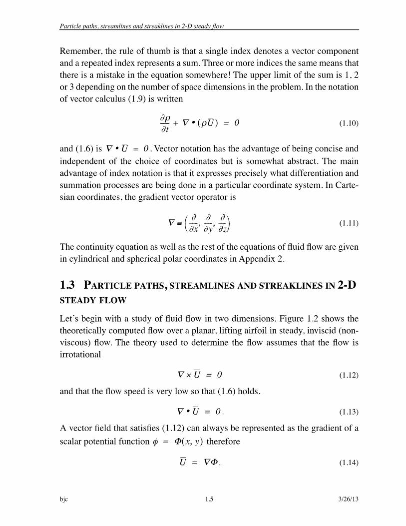
(1.38)

The expression (1.37) can now be integrated by integrating either partial deriva-tive with the appropriate variable held fixed. Let’s start by integrating the partialderivative with respect to y.

(1.39)

Note that we have to include a “constant” of integration that can be at most a func-tion of . Let . The solution can now be expressed as

(1.40)

Now differentiate (1.40) with respect to and equate to the known partial deriv-ative with respect to in (1.38).

(1.41)

This step allows us to solve for . Finally the exact solution of (1.33) is

(1.42)

Note that we had to know the integrating factor in order to solve the problem.

xyH xy( )

xy xyH xy( )+-----------------------------------–=

yx

xy xyH xy( )+-----------------------------------=

xxy xyH xy( )+-----------------------------------

x constanty f x( )+d

y=

x xy=

11 H ( )+( )

--------------------------------- f x( )+d

xy=

xx

x------ 1

1 H ( )+( )--------------------------------- f x( )+d

xy yH xy( )xy xyH xy( )+-----------------------------------–=

yxy xyH xy( )+----------------------------------- df

dx------+ yH xy( )

xy xyH xy( )+-----------------------------------–=

dfdx------ 1

x---–=

f

11 H ( )+( )

--------------------------------- xln–d

xy=


3/26/13 1.16 bjc

Sometimes what appears to be a trick will work. For example you can also get tothe solution (1.42) by simply simply defining a new variable . This allows(1.33) to be solved by separation of variables. All such tricks are equivalent tofinding the integrating factor.

In the general case the required integrating factor is not known. For example theequation

(1.43)

comes up in the study of viscous boundary layer flow along a flat plate. We knowan integrating factor exists but it has never been found.

Fortunately when it comes to streamline patterns in two dimensions, conservationof mass can be used to determine the integrating factor.

1.3.4 INCOMPRESSIBLE FLOW IN 2 DIMENSIONS

The flow of an incompressible fluid in 2-D is constrained by the continuity equa-tion (1.6) that in two dimensions reduces to

. (1.44)

This is exactly the condition (1.28) and so in this case the stream function and thevelocity field are related by

(1.45)

and is guaranteed to be a perfect differential. The integrating factoris one. Therefore one can always write for 2-D incompressible flow

. (1.46)

If and are known functions, the stream function is determined analyticallyby integration of (1.46). In practice the easiest way to assign values to the stream-lines is to integrate (1.46) at some reference state well upstream of the airfoilwhere the velocity is uniform .

xy=

dydx------ xy y y2+ +

2x2 xy–---------------------------=

xU

yV+ 0=

U y ; V x–= =

V– dx Udy+

d V– dx Udy+=

U V

U V,( ) U 0,( )=


bjc 1.17 3/26/13

1.3.5 INCOMPRESSIBLE, IRROTATIONAL FLOW IN TWO DIMENSIONS

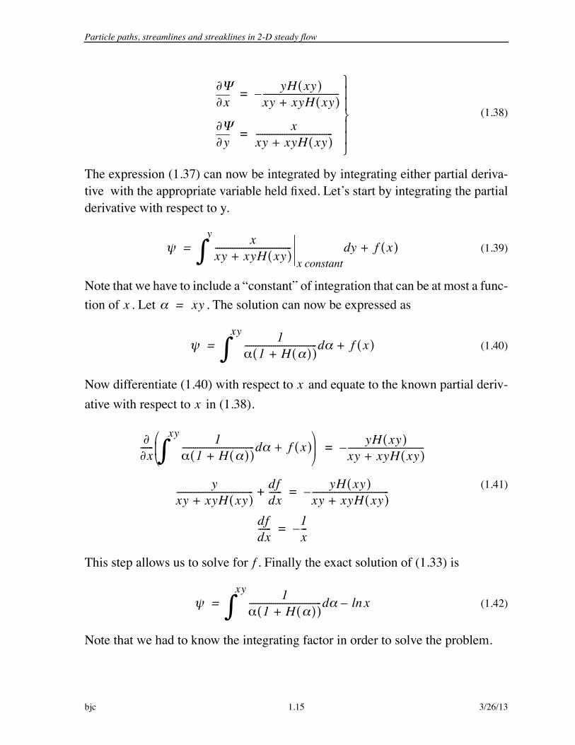
If the flow is incompressible and irrotational then the velocity field is describedby both a stream function (1.45) and a potential function (1.15). The two functionsare related by

(1.47)

These are the well known Cauchy-Riemann equations from the theory of complexvariables. Solutions of Laplace’s equation (1.16) which is the equation of motionfor this class of flows can be determined using the powerful methods of complexanalysis. Interestingly, the flow can be solved just from the continuity equation(1.13) without the use of the equation for conservation of momentum. The irrota-tionality condition (1.12) essentially supplants the need for the momentumequation.

1.3.6 COMPRESSIBLE FLOW IN 2 DIMENSIONS

The continuity equation for the steady flow of a compressible fluid in two dimen-sions is

(1.48)

In this case, the required integrating factor for (1.26) is the density andwe can write

(1.49)

The stream function in a compressible flow is proportional to the mass flux withunits and the convergence and divergence of lines in the flow overthe flap shown in Figure 1.3 is a reflection of variations in mass flux over differentparts of the flow field.

y x-------=

x–y

-------=

xU( )

yV( )+ 0=

x y,( )

d – Vdx Udy+=

mass/area-sec

Particle paths in three dimensions

3/26/13 1.18 bjc

1.4 PARTICLE PATHS IN THREE DIMENSIONS

Figure 1.6 shows the trajectory in space traced out by a particle under the actionof a general three-dimensional, unsteady flow, .

Figure 1.6 Particle trajectory in three dimensions.

Using index notation, the equations governing the motion of the particle are:

(1.50)

Formally, these equations are solved by integrating the velocity field.

(1.51)

We shall return to the discussion of flow patterns in both 2 and 3 dimensions whenwe discuss the kinematics of flow fields in Chapter 4.

1.5 THE SUBSTANTIAL DERIVATIVE

The acceleration of a particle is

. (1.52)

U x t,( )

X1

X3

X2

t=0

particle trajectory

U(x,t)x20

t=t

x10x30

dxi t( )dt

--------------- Ui x1 t( ) x2 t( ) x3 t( ) t,, ,( ) ; i 1 2 3, ,= =

xi t( ) xi0 Ui x1 t( ) x2 t( ) x3 t( ) t,, ,( ) td0

t+= ; i = 1, 2, 3

d2xi t( )

dt2------------------ d

dt-----Ui x1 t( ) x2 t( ) x3 t( ) t,, ,( )

Uit

---------Uixk

---------dxkdt

---------+= =

The substantial derivative

bjc 1.19 3/26/13

Remember, according to the Einstein convention, the repeated index denotes asum over . Use (1.50) to replace by in (1.52). The result

is called the substantial or material derivative and is usually denoted by .

. (1.53)

The substantial derivative of the velocity is

. (1.54)

The time derivative of any flow variable evaluated on a fluid element is given bya similar formula. For example the time rate of change of the density

of a given fluid particle is:

(1.55)

The substantial derivative is the time derivative of some property of a fluid ele-ment referred to a fixed frame of reference within which the fluid element movesas shown in Figure 1.6 above.

1.5.1 FRAMES OF REFERENCE

Occasionally it is necessary to transform variables between a fixed and movingset of coordinates as shown in Figure 1.7. The transformation of position andvelocity is

(1.56)

k 1 2 3, ,= dxk dt Uk

D Dt

D ( )Dt

----------- ( )t

--------- U ( )�•+=

DUiDt

-----------Uit

--------- UkUixk

---------+=

x1 t( ) x2 t( ) x3 t( ) t,, ,( )

DDt--------

t------ Uk xk

--------+=

x' x X t( )–=y' y Y t( )–=z' z Z t( )–=

U' U X t( )–=

V ' V Y t( )–=

W ' W Z t( )–=

The substantial derivative

3/26/13 1.20 bjc

where is the displacement of the moving frame in three

coordinate directions and is the velocity of theframe. Note that in general, the frame may be accelerating.

Figure 1.7 Fixed and moving frames of reference

The substantial derivative of some property of a fluid element, (1.54), (1.55), issometimes referred to as the “derivative moving with the fluid element”. Do notinterpret this as a transformation to a coordinate system that is attached to the fluidelement. If for some reason it is actually desirable to make such a transformationthe velocity of the particle in that frame is zero and the substantial derivative ofvelocity is also zero. The substantial derivative of a variable such as the densityof the particle at the origin of the moving coordinates is .

Both the momentum and kinetic energy of a fluid particle of mass depend onthe frame of reference. The momentum transforms linearly like the velocity.

(1.57)

The transformation of kinetic energy is a little more complex. In the twocoordinate systems the definition of kinetic energy is the same.

(1.58)

X X t( ) Y t( ) Z t( ), ,( )=

dX dt X t( ) Y t( ) Z t( ), ,( )=

x

y

z

x’

y’

z’

U

U(x,y,z)

V(x,y,z)

W(x,y,z)

U’

U’(x’,y’,z’)

V’(x’,y’,z’)

W’(x’,y’,z’)

X t( )

Y t( )

Z t( )

D Dt t=

m

mU' mU mdX dt–=

momentum in moving coordinates momentum in fixed coordinates

kinetic energy in moving coordinates = 12---m U'2 V '2 W '2+ +( )

Momentum transport due to convection

bjc 1.21 3/26/13

and

(1.59)

The transformation of kinetic energy between frames is

. (1.60)

which when expanded to show the kinetic energies explicitly becomes.

(1.61)

or

. (1.62)

The transformation of kinetic energy depends nonlinearly on the velocity of themoving coordinate system.

In contrast, thermodynamic properties such as density, temperature and pressureare intrinsic properties of a given fluid element and so do not depend on the frameof reference

1.6 MOMENTUM TRANSPORT DUE TO CONVECTION

The law of conservation of momentum is stated as

(1.63)

kinetic energy in fixed coordinates = 12---m U2 V 2 W2+ +( )

12---m U'2 V '2 W '2+ +( )

12---m U X–( )

2V Y–( )

2W Z–( )

2+ +( )=

12---m U'2 V '2 W '2+ +( )

12---m U2 V 2 W2+ +( ) +=

12---mX X 2U–( )

12---mY Y 2V–( )

12---mZ Z 2W–( )+ +

k' k 12---mX X 2U–( )

12---mY Y 2V–( )

12---mZ Z 2W–( )+ + +=

Rate of momentum

accumulationinside the

control volume

Rate of momentum flow

into thecontrol volume

Rate of momentum flow

out of thecontrol volume

–

Sum offorces acting

on thecontrol volume

+=


3/26/13 1.22 bjc

As a fluid moves it carries its momentum with it. This is called convective momen-tum transport. To study this kind of momentum transfer we use the samestationary control volume element that we used to develop the continu-ity equation. As before, the fluid velocity vector has components inthe directions and the fluid density is .

Figure 1.8 Fluxes of x-momentum through a fixed control volume. Arrows denote the velocity component carrying momentum into or out of the control volume.

Figure 1.8 shows the contribution to the x-momentum inside the control volumefrom the movement of fluid through all six faces of the control volume. Considera pair of faces perpendicular to the x-axis. The flux of x-momentum is withunits . The rate at which the x-component of momentumenters the face at is and the rate at which it leaves through the

face at is .

x y zU V W, ,( )

x y z, ,( )

x

z

y

x y z, ,( )

x x+ y y+ z z+, ,( )

xy

UU x

UU x x+

z

U(x,y,z,t)

V(x,y,z,t)

W(x,y,z,t)

x y z t, , ,( )

UW z

UW z z+

UV y

UV y y+

UUmomentum/area-time

x UU x y z

x x+ UU x x+ y z


bjc 1.23 3/26/13

The rate at which the x-component of momentum enters the face at is and the rate at which it leaves through the face at is

. To understand how fluid motion in the y-direction contributes

to the rate of x-momentum transfer into or out of the control volume one can makethe following interpretation of the momentum transfer.

(1.64)

Based on similar considerations, the rate at which the x-component of momentumenters the face at is and the rate at which it leaves through the

face at is .

The rate of x-component of momentum accumulation inside the control volumeis . For the x-component of momentum, the balance (1.63) isexpressed mathematically as

(1.65)

which is rearranged to read

yUV y x z y y+

UV y y+ x z

Ux-momentum

per unit volume=

V y x z

volume of fluid per second passing into the control volume through

the face normal to the V-velocitycomponent at position y

=

V y y+ x z

volume of fluid per second passing out of the control volume through

the face normal to the V-velocitycomponent at position y+ y

=

z UW z x y

z z+ UW z z+ x y

x y z U t( )

x y z Ut

----------- y z UU x y z UU x x+– +=

x z UV y x z UV y y+– x y UW z x y UW z z+– + +

the sum of x-component forces acting on the system{ }


3/26/13 1.24 bjc

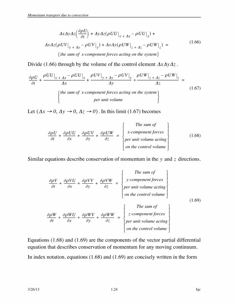
(1.66)

Divide (1.66) through by the volume of the control element .

(1.67)


(1.68)

Similar equations describe conservation of momentum in the and directions.

(1.69)

Equations (1.68) and (1.69) are the components of the vector partial differentialequation that describes conservation of momentum for any moving continuum.

In index notation, equations (1.68) and (1.69) are concisely written in the form

x y z Ut

----------- y z UU x x+ UU x–( ) + +

x z UV y y+ UV y–( ) x y UW z z+ UW z–( )+ =

the sum of x-component forces acting on the system{ }

x y z

Ut

-----------UU x x+ UU x–

x------------------------------------------------------

UV y y+ UV y–

y----------------------------------------------------- +

UW z z+ UW z–

z------------------------------------------------------+ + =

the sum of x-component forces acting on the systemper unit volume

x 0 y 0 z 0, ,( )

Ut

----------- UUx

---------------- UVy

---------------- UWz

-----------------+ + +

The sum ofx-component forces

per unit volume actingon the control volume

=

y z

Vt

----------- VUx

--------------- VVy

--------------- VWz

----------------+ + +

The sum ofy-component forces


=

Wt

------------ WUx

----------------- WVy

---------------- WWz

-----------------+ + +

The sum ofz-component forces


=


bjc 1.25 3/26/13

(1.70)

where the subscript refers to the -th vector component and the sum is over therepeated index . Since the repeated index is always summed it makes no differ-ence what symbol is used and so it is called a dummy index.

Rearrange (1.70) by carrying out the indicated differentiation.

(1.71)

The term in parentheses on the left hand side of (1.71) is zero by continuity andso the momentum equation becomes

. (1.72)

Equation (1.72) can be stated in words as follows.

(1.73)

Equation (1.72) clearly shows the connection between conservation of momen-tum for fluid motion and the classical Newton’s law .

Uit

-------------UiU j( )

x j-------------------------+

Sum of theith-component forcesper unit volume actingon the control volume

; i = 1,2,3=

ij

Uit

--------- U jUi( )

x j-------------- Ui t

------U j( )

x j-------------------++ +

The sum ofith-component forcesper unit volume actingon the control volume

=

DUiDt

-----------

The sum ofith-component forcesper unit volume actingon the control volume

=

The rate of momentum changeof a fluid element

The vector sum offorces acting

on the fluid element=

ma F=

Momentum transport due to molecular motion at microscopic scales

3/26/13 1.26 bjc

1.7 MOMENTUM TRANSPORT DUE TO MOLECULAR MOTION AT MICROSCOPIC SCALES

Appendix I describes the molecular origin of two of the most basic forces that acton a fluid element; pressure and viscous friction. Although the derivations arerestricted to gases, both types of forces exist in all fluid motion and both arise frommomentum transfer due to the motion and collisions of the molecules that makeup the fluid. Molecules in the fluid move in random and chaotic ways and acrossany selected section of a surface within the fluid there are molecules moving inboth directions through the surface. The pressure and viscosity are definedthrough an average of the momentum transfer due to the collective motion of avery large set of molecules over a time scale that is short compared to the unsteadymacroscopic motion of the fluid.

1.7.1 PRESSURE

Pressure forces arise from collisions between the molecules within the fluid andwith whatever form of containment is used to hold or bound the fluid. In a fluidat rest, in the absence of gravitational forces, the pressure is uniform everywhere.When the fluid is set into motion the pressure becomes a scalar function of spaceand time. For example, variations in the pressure over a wing give rise to the liftof the wing. Pressure variations in the atmosphere are the primary driving forcebehind wind patterns. The drag of a motor vehicle is primarily due to variationsin the pressure field over the surface of the vehicle.

1.7.2 VISCOUS FRICTION - PLANE COUETTE FLOW

All simple fluids exhibit resistance to flow due to the physical property of viscos-ity. The effects of viscosity are readily apparent in many everyday activities suchas the spreading of honey on a piece of bread or the slow dripping of paint froma brush. Anyone who has purchased oil for their car knows that different gradesof oil are characterized by different viscosities and that the viscosity depends onthe oil temperature. The viscosity of air and other gases is less apparent but none-theless just as real. The most important effect of viscosity on the motion of a fluidis that it causes the fluid to stick to the surface of a moving solid body imposingthe so-called no-slip condition on the velocity field at the surface. Even thoughthe viscosity of air may be very small, viscous forces profoundly affect the flowand are critical to the generation of lift and drag by moving bodies.


bjc 1.27 3/26/13

To illustrate viscous friction consider a fluid contained between two large parallelplates with area as shown in Figure 1.9 below. The fluid is initially at rest. At

the upper plate is set into motion and, due to viscous forces, the adjacentfluid layers are dragged along with it. Eventually the velocity field reaches asteady state. If the speed of the upper plate is small compared to the speed ofsound in the fluid the final velocity profile is a straight line as shown.

This is called plane Couette flow after Maurice Frederic Alfred Couette a Profes-sor of Physics at the French University of Angers at the end of the nineteenthcentury. Couette actually studied the flow between inner and outer concentricrotating cylinders with the goal of using his device to measure viscosity.

Figure 1.9 Build-up to a steady laminar velocity profile for a vis-cous fluid contained between two parallel plates. At t=0 the upper plate is set into motion at a constant speed .

At 0=

x

y

x

y

x

y

x

y U

U

U

t < 0

t = 0+

Small t

Large t

Fluid all at rest

Upper plate set in motion

Unsteady velocity increase

Steady state velocity distribution

U(y,t)

U(y)

d

n

U


3/26/13 1.28 bjc

Once the flow reaches steady state a constant force is required to maintain themotion of the upper plate. Provided the flow is laminar and the plate speed is nottoo large the force may be expressed as

(1.74)

The viscous stress on the plate ( ) is proportional to the velocity gradi-ent and the constant of proportionality is the viscosity of the fluid.

Later we will generalize the notion of viscous stress to flow in three dimensionsand so it is useful to write (1.74) in a somewhat more general form. The shearstress acting in the direction exerted on a layer of fluid with an outward unitnormal vector in the positive direction (as shown) is designated . In terms

of the velocity derivative (1.74) is written,

. (1.75)

Equation (1.75) is called Newton’s law of viscosity after Sir Isaac Newton whofirst proposed it.

In Chapter 5 we will consider the compressible case where the plate speed is notsmall and the steady-state velocity profile deviates from a straight line.

1.7.3 A QUESTION OF SIGNS

There is a subtle sign issue that comes up when one defines the viscous stress. Inthe discussion just above we have adopted the convention normally used in aero-nautics that the stress is the force on a surface defined by its outward normalvector. In Figure 1.9 the outward normal on the lower surface is positive and theforce is in the positive x-direction; on the upper surface the force is in the negativex-direction on a surface defined by an outward normal that points in the negativey-direction. Either way is positive as indicated in (1.75).

But in certain fields such as chemical engineering a different interpretation of thestress is used. Here the stress is viewed as the transport of momentum in a certaindirection. In this view the flow in Figure 1.9 would be interpreted as the transportof positive x-momentum in the negative y-direction and the expression in (1.75)

F

FA--- µ

Ud

--------=

force/area

xn y xy

xy µdUdy-------=

xy


bjc 1.29 3/26/13

would have a negative sign. If the general momentum conservation equation isdeveloped with this interpretation of stress then another negative sign appears infront of the stress term. When the constitutive relation between stress and rate-of-strain is introduced both camps wind up solving the same system of equations.

1.7.4 NEWTONIAN FLUIDS

A fluid for which the viscous stress is linearly proportional to the velocity gradientis called Newtonian. Virtually all gases and most liquids are Newtonian. The fewexceptions include polymers, pastes and slurries that exhibit non-Newtonianbehavior where the stress depends nonlinearly on the rate of strain and mayexhibit dependence on the total strain as in a solid. Some fluids are said to havememory where the stress can depend on the past history of the rate-of-strain. Wewill introduce the Newtonian stress-rate-of-strain relation in Chapter 5. For thepresent the stress is left in general terms.

A truly exceptional case is liquid Helium that, when cooled to below 2.3°K,undergoes a transition to a strange macroscopic quantum state called Helium II.A given sample of Helium below this temperature consists of two fluids thatappear to co-exist. The normal fluid component exhibits viscosity whereas thesuperfluid component appears to flow without any viscous friction. In fact HeliumII is an extraordinarily difficult fluid to contain since the superfluid componentcan pass through ultrafine leaks in the dewar used to hold it.

Exceptions to the no-slip condition occur in the flow of highly rarefied gases suchas in the upper reaches of the atmosphere during re-entry of a space craft. Whenthe density of the gas is extremely low the fluid can no longer be treated as a con-tinuous medium. In this case the flow must be treated by modeling the motion andcollisions of individual molecules. Near a wall molecular collisions may not beperfectly specular and may on average exhibit a small difference between thevelocity of the surface and the mean velocity of fluid particles near the surface.This is called the slip velocity and can become quite large as the density of thegas decreases to extremely low values.


3/26/13 1.30 bjc

1.7.5 FORCES ACTING ON A FLUID ELEMENT

At macroscopic scales the transport of momentum due to the net molecularmotion of a very large number of molecules is equivalent to continuous pressureand viscous forces acting within the fluid. Figure 1.10 below shows the contribu-tion to the x-momentum inside our small control volume from the pressure andviscous stresses acting on the six faces of the control volume.

Figure 1.10 Pressure and viscous stresses acting in the x-direction

Consider a pair of faces perpendicular to the x-axis in Figure 1.10. The force onthe face the face at with outward normal in the negative x-direction is

and the force on the face at with outward normal in

the positive x-direction is . The x-component of force on

the face at due to viscous stress is and the x-component of force

x

z

y

x y z, ,( )

x x+ y y+ z z+, ,( )

xy

P– + xx( )x

P– + xx( )x x+

z

xz z

xz z z+

xy y

xy y y+

xP– + xx( )–

xy z x x+

P– + xx( )x x+

y z

y – xy yx z


bjc 1.31 3/26/13

on the face at is . Finally, the x-component of force on

the face at is and the x-component of force on the face at

is . Note that the pressure is a scalar that acts normal to any sur-

face in the fluid and therefore there is no component of the pressure acting in thex-direction on the faces perpendicular to the and directions. The pressure-viscous stress forces acting in all three directions on the control volume are

(1.76)

With convection, pressure and viscous forces included, the x-component momen-tum balance over the control volume is, from (1.65)

y y+ xy y y+x z

z – xz zy z z z+

xz z z+y z

y z

Fx y z P– + xx( )x x+

P– + xx( )–x

x z xy y y+–

xy y + +=

x y xz z z+–

xz z

Fy y z xy x x+–

xy xx z P– + yy( )

y y+P– + yy( )–

y + +=

x y yz z z+–

yz z

Fz y z xz x x+–

xz xx z yz y y+

–yz y

+ +=

x y P– + zz( )z z+

P– + zz( )–z


3/26/13 1.32 bjc

. (1.77)

Divide (1.77) through by and move the pressure and viscous stress termsto the left hand side. The result is

(1.78)


(1.79)

The equations for conservation of momentum in the and directions are derivedin a similar way using the expressions in (1.69) and (1.76).

(1.80)

In index form, using the Einstein convention, the momentum conservation equa-tion is

x y z Ut

----------- y z UU x UU x x+–( ) +=

x z UV y UV y y+–( ) x y UW z UW z z+–( ) + +

y z P– + xx( )x x+

P– + xx( )–x

+

x z xy y y+–

xy yx y xz z z+

–xz z

+

x y z

Ut

-----------UU x x+ UU x– P xx–( )

x x+P xx–( )

x–+

x---------------------------------------------------------------------------------------------------------------------------------------- + +

UV y y+ UV y– xy y y+ xy y––

y------------------------------------------------------------------------------------------------------------- +

UW z z+ UW z– xz z z+ xz z––

z------------------------------------------------------------------------------------------------------------- 0=

x 0 y 0 z 0, ,( )

Ut

-----------UU P xx–+( )

x----------------------------------------------

UV xy–( )

y-----------------------------------

UW xz–( )

z------------------------------------+ + + 0=

y z

Vt

-----------VU xy–( )

x-----------------------------------

VV P yy–+( )

y---------------------------------------------

VW yz–( )

z-----------------------------------+ + + 0=

Wt

------------WU xz–( )

x------------------------------------

WV yz–( )

y-----------------------------------

WW P zz–+( )

z-----------------------------------------------+ + + 0=

Conservation of energy

bjc 1.33 3/26/13

. (1.81)

The coordinate independent form of (1.81) is

. (1.82)

The tensor product of vectors that appears in (1.82), , also called a

dyadic product, is sometimes written . Fully written out, this product is

. (1.83)

Note that the matrix (1.83) is symmetric and as we shall see in Chapter 5, so isthe stress tensor .

1.8 CONSERVATION OF ENERGY

The law of conservation of energy is stated as

(1.84)

The energy per unit mass of a moving continuum is where is the internalenergy per unit mass and

Uit

-------------UiU j( )

x j------------------------- P

xi------- ij

x j---------–+ + 0 ; i = 1,2,3=

Ut

----------- UU( )�• P �•–+ + 0=

UU UiU j=

U U

UUUU UV UWVU VV VWWU WV WW

=

ij

Rate of energy

accumulationinside the

control volume

Rate of energy flow

into thecontrol volumeby convection

Rate of energy flowout of the

control volumeby convection

– +=

Work done on thecontrol volumeby pressure andviscous forces

Rate of energyaddition due toheat conduction

Energy generationdue to sources

inside thecontrol volume

+ +

e k+ e


3/26/13 1.34 bjc

(1.85)

is the kinetic energy per unit mass. The convection of energy into and out of thecontrol volume is depicted in Figure 1.11.

Figure 1.11 Convection of energy into and out of a control volume.

1.8.1 PRESSURE AND VISCOUS STRESS WORK

The forces that act on the surface of a control volume do work on the fluid in thecontrol volume and therefore contribute to the energy balance. The power (energyper second) put into the fluid within the control volume is given by the classicalrelation from mechanics

(1.86)

Where is the flow velocity and is the net vector force on the control volumeby pressure and viscous forces with components (1.76). Fully written out (1.86) is

k 1 2( ) U2 V 2 W2+ +( )=

x

z

y

x y z, ,( )

x x+ y y+ z z+, ,( )

xy

e k+( )U x

e k+( )U x x+

z

U(x,y,z,t)

V(x,y,z,t)

W(x,y,z,t)

e k+( )W z

e k+( )W z z+

e k+( )V y

e k+( )V y y+

Power input to the control volume = F U�•

U F


bjc 1.35 3/26/13

(1.87)

The right-hand-side of (1.87) can be parsed into a series of energy fluxes into andout of the various faces of the control volume.

(1.88)

The contribution of these fluxes to the energy balance over the control volume isillustrated in Figure 1.12.

Power input to the control volume =

y z P– + xx( )x x+

P– + xx( )–x

U xy x x+–

xy xV + +

xz x x+–

xz xW +

x z xy y y+–

xy yU P– + yy( )

y y+P– + yy( )–

yV + +

yz y y+–

yz yW +

x y xz z z+–

xz zU yz z z+

–yz z

V + +

P– + zz( )z z+

P– + zz( )–z

W

Power input to the control volume =

y z PU– xxU xyV xzW+ + +( )x x+

PU– xxU xyV xzW+ + +( )–x

+

x z PV– xyU yyV yzW+ + +( )y y+

PV– xyU yyV yzW+ + +( )–y

+

x y PW– zxU zyV zzW+ + +( )z z+

PW– zxU zyV zzW+ + +( )–z


3/26/13 1.36 bjc

Figure 1.12 Energy fluxes due to the work done on the control volume by pressure and viscous forces.

In addition to the energy input due to work done by pressure and viscous forcesone must also include the flux of heat into and out of the control volume dueto thermal conduction.

The rate of internal and kinetic energy accumulation inside the control volume is. With all the various sources of energy taken into

account, the energy balance (1.84) is expressed mathematically as

x

z

y

x y z, ,( )

x x+ y y+ z z+, ,( )

xy

PU– xxU xyV xzW+ + +( )x

PU– xxU xyV xzW+ + +( )x x+

z

PW– zxU zyV zzW+ + +( )z

PW– zxU zyV zzW+ + +( )z z+

PV– xyU yyV yzW+ + +( )y

PV– xyU yyV yzW+ + +( )y y+

Q

x y z e k+( ) t( )


bjc 1.37 3/26/13

(1.89)

Divide (1.89) through by the infinitesimal volume and take the limit. The conservation equation for the energy becomes

(1.90)

In index form the energy conservation equation is

. (1.91)

and the coordinate independent form of (1.91) is

. (1.92)

x y z e k+( )t

------------------------- y z e k+( )U x e k+( )U x x+–( ) +=

x z e k+( )V y e k+( )V y y+–( ) +

x y e k+( )W z e k+( )W z z+–( ) +

y z PU– xxU xyV xzW+ + +( )x x+

PU– xxU xyV xzW+ + +( )–x

x z PV– xyU yyV yzW+ + +( )y y+

PV– xyU yyV yzW+ + +( )–y

x y PW– zxU zyV zzW+ + +( )z z+

PW– zxU zyV zzW+ + +( )–z

+

y z Qx xQx x x+

– x z Qy yQy y y+

– x y Qz zQz z z+

– + + +

Power generation due to sources inside the control volume{ }

x y zx 0 y 0 z 0, ,( )

e k+( )t

------------------------- e k+( )U( )x

----------------------------------- e k+( )V( )y

---------------------------------- e k+( )W( )z

------------------------------------ + + + +

PU xx– U xy– V xz– W( )

x------------------------------------------------------------------

PV xy– U yy– V yz– W( )

y------------------------------------------------------------------ + +

PW zx– U zy– V zz– W( )

z------------------------------------------------------------------

Qxx

----------Qyy

----------Qzz

---------+ + + =

Power generation due to sources inside the control volume{ }

e k+( )t

-------------------------e k+( )U j( )

x j-------------------------------------

PU jx j

--------------Ui ij( )

x j---------------------–

Q jx j

----------+ + + Power sources{ }=

e k+( )t

------------------------ e k+( )U PU U�•– Q+ +( )�•+ Power sources{ }=

Summary - the equations of motion

3/26/13 1.38 bjc

Power sources within the control volume can take on a wide variety of formsincluding chemical reactions, phase change, light absorption from an externalsource, nuclear reactions, etc.

1.9 SUMMARY - THE EQUATIONS OF MOTION The combined conservation equations in Cartesian coordinates are

. (1.93)

See Appendix 2 for the equations of motion in cylindrical and spherical polarcoordinates.

In their current form (1.93) the equations cannot be solved until there is an addi-tional equation that relates the viscous stresses to the velocity field. In Chapter 5the general form of the Newtonian constitutive law (1.75) will be defined.


t------ U

x----------- V

y----------- W

z------------+ + + 0=

Conservation of momentum

Ut

-----------UU P xx–+( )

x----------------------------------------------

UV xy–( )

y-----------------------------------

UW xz–( )

z------------------------------------+ + + 0=

Vt

-----------VU xy–( )

x-----------------------------------

VV P yy–+( )

y---------------------------------------------

VW yz–( )

z-----------------------------------+ + + 0=

Wt

------------WU xz–( )

x------------------------------------

WV yz–( )

y-----------------------------------

WW P zz–+( )

z-----------------------------------------------+ + + 0=


e k+( )t

------------------------- e k+( )U( )x

----------------------------------- e k+( )V( )y

---------------------------------- e k+( )W( )z

------------------------------------ + + + +

PU xx– U xy– V xz– W( )

x------------------------------------------------------------------

PV xy– U yy– V yz– W( )

y------------------------------------------------------------------ + +

PW zx– U zy– V zz– W( )

z------------------------------------------------------------------

Qxx

----------Qyy

----------Qzz

---------+ + + Power sources{ }=

Problems

bjc 1.39 3/26/13

Also required is a way of relating the density and pressure that appear in themomentum equation to the internal energy that appears in the energy equation.This will come from thermodynamics and the definition of an equation of state.The heat flux in the energy equation will be related to the fluid temperature usingFick’s law for linear heat conduction.

Inclusion of these relations leads to a closed system of governing equations forviscous compressible flow where the number of equations is equal to the numberof unknowns. Under certain flow assumptions that are of considerable aeronauti-cal interest it will be possible to directly relate the density and pressure withouthaving to know the temperature. In this case the momentum and mass conserva-tion equations become a closed system that is sufficient to fully describe the flow.The two most common cases where this occurs are incompressible flow where thedensity is constant and isentropic compressible flow where the pressure is relatedto the density by a power law.

1.10 PROBLEMS

Problem 1 - Show that the continuity equation can be expressed as

(1.94)

Problem 2 - Use direct measurements from the streamline figure below to esti-mate the percent change from the free stream velocity at points , , and .

1---DDt--------

U jx j

----------+ 0=

A B C D

A

B

C

D

Problems

3/26/13 1.40 bjc

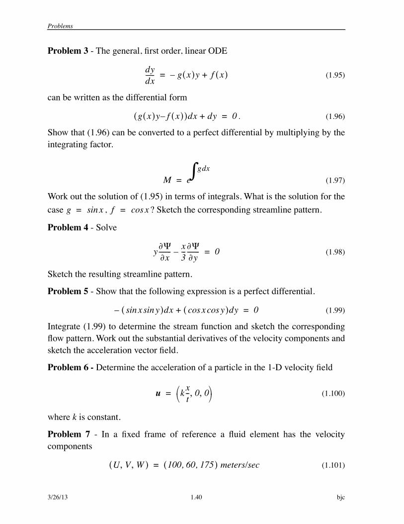
Problem 3 - The general, first order, linear ODE

(1.95)

can be written as the differential form

. (1.96)

Show that (1.96) can be converted to a perfect differential by multiplying by theintegrating factor.

(1.97)

Work out the solution of (1.95) in terms of integrals. What is the solution for thecase , ? Sketch the corresponding streamline pattern.

Problem 4 - Solve

(1.98)

Sketch the resulting streamline pattern.

Problem 5 - Show that the following expression is a perfect differential.

(1.99)

Integrate (1.99) to determine the stream function and sketch the correspondingflow pattern. Work out the substantial derivatives of the velocity components andsketch the acceleration vector field.

Problem 6 - Determine the acceleration of a particle in the 1-D velocity field

(1.100)

where k is constant.

Problem 7 - In a fixed frame of reference a fluid element has the velocitycomponents

(1.101)

dydx------ g x( )y– f x( )+=

g x( )y f– x( )( )dx dy+ 0=

M eg xd

=

g xsin= f xcos=

y x-------- x

3---

y--------– 0=

x ysinsin( )dx– x ycoscos( )dy+ 0=

u k xt-- 0 0, ,=

U V W, ,( ) 100, 60, 175( ) meters/sec=

Problems

bjc 1.41 3/26/13

Suppose the same fluid element is observed in a frame of reference moving at

(1.102)

with respect to the fixed frame. Determine the velocity components measured bythe observer in the moving frame. Determine the kinetic energy per unit mass ineach frame.

Problem 8 - The stream function of a steady, 2-D compressible flow in a cor-ner is shown below.

Determine plausible expressions for the velocity components and densityfield. Does a pressure field exist for this flow if it is assumed to be inviscid?

Problem 9 - The expansion into vacuum of a spherical cloud of a monatomic gassuch as helium has a well-known exact solution of the equations for compressibleisentropic flow. The velocity field is

. (1.103)

The density and pressure are

. (1.104)

where is the initial radius of the cloud. This problem has served as a

model of the expanding gas nebula from an exploding star.

1) Determine the particle paths .

X 25, 110, 90( ) meters/sec=

xy1 x y+ +-----------------------=

U xt

t02 t2+

---------------= V yt

t02 t2+

---------------= W zt

t02 t2+

---------------=

0------

t03

t02 t2+( )

3 2------------------------------ 1

t02

Rinitial2------------------ x2 y2 z2+ +

t02 t2+

-------------------------------–

3 2

=

pp0------

0------

5 3=

Rinitial

x t( ) y t( ) z t( ),,( )

Problems

3/26/13 1.42 bjc

2) Work out the substantial derivative of the density .

Problem 10 - A moving fluid contains a passive non-diffusing scalar contaminantSmoke in a wind tunnel would be a pretty good example of such a contaminant.Let the concentration of the contaminant be The units of are

(1.105)

Derive a conservation equation for .

Problem 11 - Include the effects of gravity in the equations of motion (1.93). Youcan check your answer with the equations derived in Chapter 5.

D Dt

C x y z t, , ,( ) C

mass of contaminant/unit mass of fluid

C

C 1 I NTRODUCTION TO F LUID F LOW - Stanford …cantwell/AA200_Course_Material/... ·...

Documents

Transcript of C 1 I NTRODUCTION TO F LUID F LOW - Stanford …cantwell/AA200_Course_Material/... ·...