by

Roger Pynn

Los Alamos National Laboratory

LECTURE 5: Small Angle Scattering

This Lecture

5. Small Angle Neutron Scattering (SANS)1. What is SANS and what does it measure?2. Form factors and particle correlations3. Guinier approximation and Porod’s law4. Contrast and contrast variation5. Deuterium labelling6. Examples of science with SANS

1. Particle correlations in colloidal suspensions2. Helium bubble size distribution in steel3. Verification of Gaussian statistics for a polymer chain in a melt4. Structure of 30S ribosome5. The fractal structure of sedimentary rocks

Note: The NIST web site at www.ncnr.nist.gov has several good resources for SANS – calculations of scattering length densities & form factors as well as tutorials

Small Angle Neutron Scattering (SANS) Is Used to Measure Large Objects (~1 nm to ~1 µm)

• Complex fluids, alloys, precipitates,biological assemblies, glasses,ceramics, flux lattices, long-wave-length CDWs and SDWs, criticalscattering, porous media, fractalstructures, etc

Scattering at small angles probeslarge length scales

Two Views of the Components of a Typical Reactor-based SANS Diffractometer

The NIST 30m SANS Instrument Under Construction

Where Does SANS Fit As a Structural Probe?

• SANS resolves structures on length scales of 1 – 1000 nm

• Neutrons can be used with bulk samples (1-2 mm thick)

• SANS is sensitive to light elements such as H, C & N

• SANS is sensitive to isotopes such as H and D

What Is the Largest Object That Can Be Measured by SANS?

• Angular divergence of the neutron beam and its lack of monochromaticity contribute to finite transverse & longitudinal coherence lengths that limit the size of an object that can be seen by SANS

• For waves emerging from slit center,path difference is hd/L if d<<h<<L;for waves from one edge of the slit path difference is (h+a)d/L

• The variation of path difference, whichcauses decreased visibility of Young’sfringes, is ad/L so the variation in phasedifference is ∆ψ = kad/L

• To maintain the visibility of the Young’sinterference pattern we ∆ψ ∼ 2π so thecoherence length, d ~ λ/α where α is thedivergence angle a/L

• The coherence length is the maximum distance between points in a scatterer for which interference effects will be observable

+a

-a

d

L

r1

r2 h

Instrumental Resolution for SANSTraditionally, neutron scatterers tend to think in terms of Q and E resolution

dominates. resolutionh wavelengtsample, thefrom distance and sizedetector by theset , of lueslargest va at the that Note

neutrons. Å 15 using instrument SANS m 40 ILL at the m 5about of maximum a

achieves andneutron for thelength coherence e transvers the toequal is This

. /~Q/2~ isobject observablelargest The /)/2(~/4~)Q/(~Q

and dominates resolutionangular , of valueAt this/5.1~ :size beamdirect by the determined is of aluesmallest v The

h/L.12/5 h, of sample and sourceat apertures

equal and L of distancesdetector -sample & sample-source equalFor

0025.0 so small, is and 5% ~ )/( SANS,For

sin.cos

sin4

rms

rmsminminrmsrms

min

2

22

2

2

22

2

22

2

θµ

λδπλπλπδθθδθδ

θθθ

δθ

θδθδ

θλδλ

θδθθ

λδλδ

θλπ

LhLh

Lh

QQ

QQ

Q

rms

rms

=

+=

+=⇒=

The Scattering Cross Section for SANS

• Since the length scale probed at small Q is >> inter-atomic spacing we may use the scattering length density (SLD), ρ, introduced for surface reflection and note that nnuc(r)b is the local SLD at position r.

• A uniform scattering length density only gives forward scattering (Q=0), thus SANS measures deviations from average scattering length density.

• If ρ is the SLD of particles dispersed in a medium of SLD ρ0, and np(r) is the particle number density, we can separate the integral in the definition of S(Q) into an integral over the positions of the particles and an integral over a single particle. We also measure the particle SLD relative to that of the surrounding medium I.e:

densitynuclear

theis andlength scatteringnuclear coherent theis where

)(.1

)( where)( that recall

2

2.2

)r(nb

rnerdN

QSQNSbdOds

nuc

nucrQi

r

rrrr rr

∫ −==

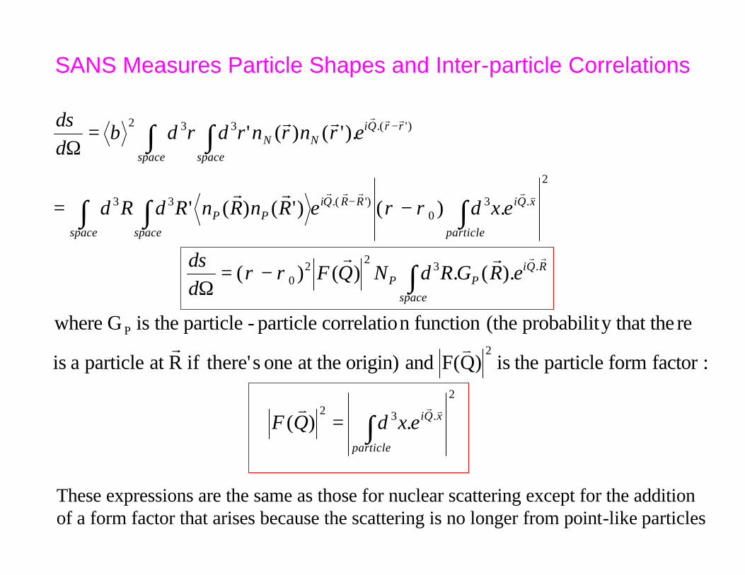
SANS Measures Particle Shapes and Inter-particle Correlations

2

.32

2

P

.3220

2

.30

)'.(33

)'.(332

.)(

:factor form particle theis )QF( and origin) at the one s there'if Rat particle a is

rey that theprobabilit (thefunction n correlatio particle-particle theis G where

).(.)()(

.)()'()('

).'()('

∫

∫

∫∫ ∫

∫ ∫

=

−=Ω

−=

=Ω

−

−

particle

xQi

RQiP

spaceP

particle

xQiRRQi

space spacePP

rrQi

space spaceNN

exdQF

eRGRdNQFdd

exdeRnRnRdRd

ernrnrdrdbdd

vr

rr

vrrrr

rrr

v

vr

rr

rr

rr

ρρσ

ρρ

σ

These expressions are the same as those for nuclear scattering except for the additionof a form factor that arises because the scattering is no longer from point-like particles

Scattering for Spherical Particles

particles. ofnumber thetimes volumeparticle theof square the toalproportion is )]r( )rG( when [i.e. particles

spherical eduncorrelat ofassembly an from scattering total the0,Q as Thus,

0Qat )(3

)(cossin

3)(

:Q of magnitude on the dependsonly F(Q) R, radius of sphere aFor

shape. particle by the determined is )(factor form particle The

010

30

2

.2

vr

rr rr

δ→→

=→≡

−=

= ∫

VQRjQRV

QRQRQRQR

VQF

erdQF

sphere

V

rQi

2 4 6 8 10

0.2

0.4

0.6

0.8

1

3j1(x)/x

xQ and (a) axismajor the

between angle theis where)cossin (

:by R replace particles ellipticalFor

2/12222

rϑ

ϑϑ baR +→

Examples of Spherically-Averaged Form Factors

H

R

R

r

t = R - r

Fo rm Fact or fo r a Ve s ic le

)()()(3),,(

3321

21

2

0 rRQQrjrQRjRVrRQF

−−=

Form Factor for Cylinder with Q at angle θ to cylinder axis

210

)sin(cos)sin()cos]2/sin([4

),,,(θθ

θθθ

QRQHQRJQHV

RHQF =

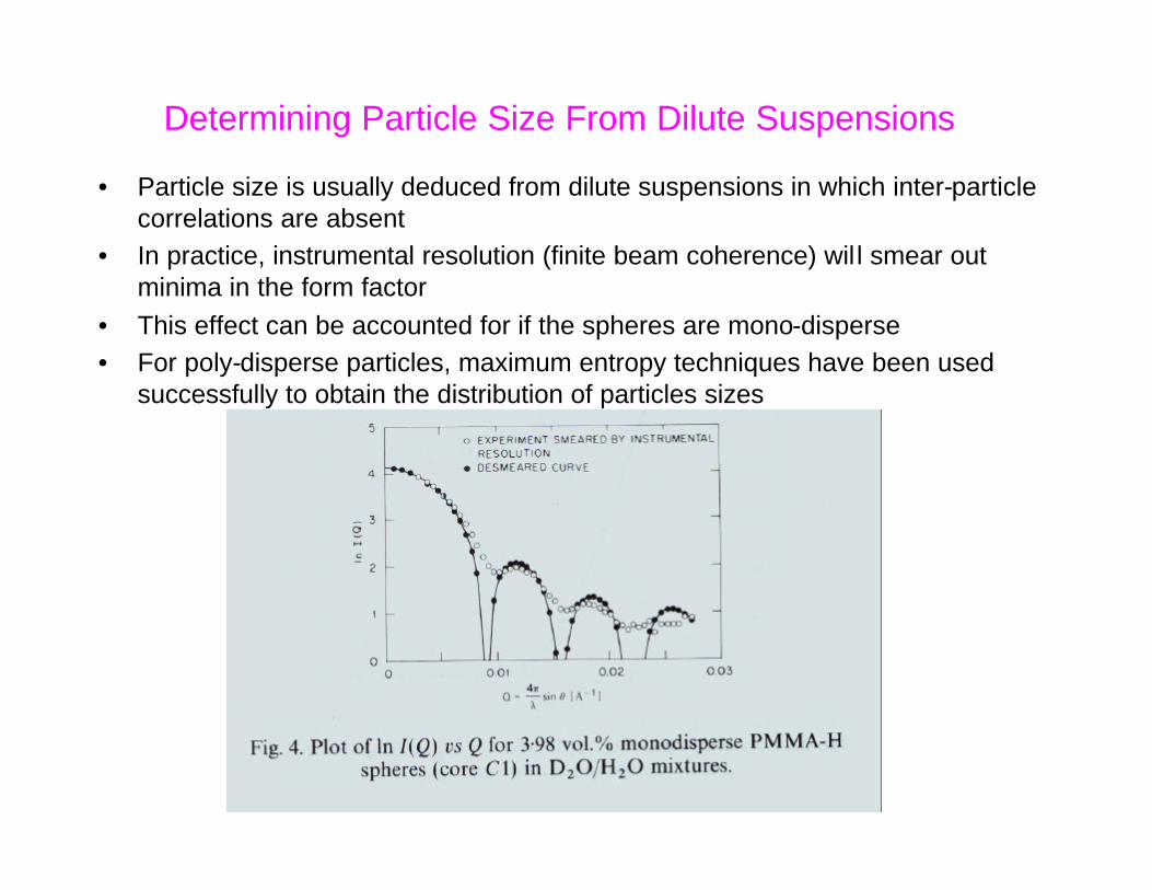
Determining Particle Size From Dilute Suspensions

• Particle size is usually deduced from dilute suspensions in which inter-particle correlations are absent

• In practice, instrumental resolution (finite beam coherence) wil l smear out minima in the form factor

• This effect can be accounted for if the spheres are mono-disperse • For poly-disperse particles, maximum entropy techniques have been used

successfully to obtain the distribution of particles sizes

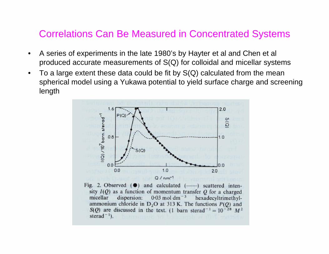
Correlations Can Be Measured in Concentrated Systems

• A series of experiments in the late 1980’s by Hayter et al and Chen et al produced accurate measurements of S(Q) for colloidal and micellar systems

• To a large extent these data could be fit by S(Q) calculated from the mean spherical model using a Yukawa potential to yield surface charge and screening length

Size Distributions Have Been Measured for Helium Bubbles in Steel

• The growth of He bubbles under neutron irradiation is a key factor limiting the lifetime of steel for fusion reactor walls– Simulate by bombarding steel with alpha particles

• TEM is difficult to use because bubble are small• SANS shows that larger bubbles grow as the steel is

annealed, as a result of coalescence of small bubblesand incorporation of individual He atoms

SANS gives bubble volume (arbitrary units on the plots) as a function of bubble size at different temperatures. Red shading is 80% confidence interval.

Radius of Gyration Is the Particle “Size” Usually Deduced From SANS Measurements

result. general thisof case special a is sphere a offactor form for the expression

that theifiedeasily ver isIt /3.r is Q of ueslowest val at the data theof slope The

.Q vty)ln(Intensi plottingby or region)Guinier called-so (in the Q lowat data SANS to

fit a from obtainedusually isIt ./ isgyration of radius theis r where

...6

1....sin

.sincos

21

....).(21

.)(

:Q smallat factor form theof definition in the lexponentia theexpand and particle theof centroid thefrom measure weIf

2g

2

332g

60

22

03

32

0

0

22

0

3230

.

22

∫∫

∫

∫

∫

∫

∫∫∫

=

≈

+−=

+−=

+−+≈=

−

VVg

rQg

V

V

VV

rQi

V

rdrdRr

eVrQ

Vrd

rdr

d

dQ

V

rdrQrdrQiVerdQF

r

g

π

π

θθ

θθθ

rrrrr

r

rr

2

Guinier Approximations: Analysis Road Map

• Guinier approximations provide a roadmap for analysis.

• Information on particle composition, shape and size.

• Generalization allows for analysis of complex mixtures, allowing identification of domains where each approximation applies.

P(Q) = 1; α = 0

απ Q–α; α = 1,2∆Mα0 exp –

Rα2 Q2

3 – α

d ln P(Q)d ln(Q) = Q

P(Q)d P(Q)

dQ = –α – 23 – α Rα

2 Q2

Generalized Guinier approximation

Derivative-log analysis

* Viewgraph courtesy of Rex Hjelm

Contrast & Contrast Matching

Both tubes contain borosilicate beads + pyrex fibers + solvent. (A) solvent refractive index matched to pyrex;. (B) solvent index different from both beadsand fibers – scattering from fibers dominates

O

O

Wat

erD2O

H2O

* Chart courtesy of Rex Hjelm

Isotopic Contrast for Neutrons

HydrogenIsotope

Scattering Lengthb (fm)

1H -3.7409 (11)2D 6.674 (6)3T 4.792 (27)

NickelIsotope

Scattering Lengthsb (fm)

58Ni 15.0 (5)60Ni 2.8 (1)

61Ni 7.60 (6)

62Ni -8.7 (2)

64Ni -0.38 (7)

Verification of of the Gaussian Coil Model for a Polymer Melt

• One of the earliest importantresults obtained by SANS was the verification of that rg~N-1/2

for polymer chains in a melt

• A better experiment was done3 years later using a smallamount of H-PMMA in D-PMMA(to avoid the large incoherentbackground) covering a MW range of 4 decades

SANS Has Been Used to Study Bio-machines

• Capel and Moore (1988) used the fact that prokaryotes can grow when H is replacedby D to produce reconstituted ribosomes with various pairs of proteins (but not rRNA) deuterated

• They made 105 measurements of inter-protein distances involving 93 30S proteinpairs over a 12 year period. They alsomeasured radii of gyration

• Measurement of inter-protein distancesis done by Fourier transforming the formfactor to obtain G(R)

• They used these data to solve the ribosomal structure, resolving ambiguitiesby comparison with electron microscopy

Porod Scattering

function.n correlatio for the form (Debye) h thisfactor wit form theevaluate toandr smallat V)]A/(2 a[with ..brar-1G(r) expand toisit obtain y toAnother wa

smooth. is surfaceparticle theprovided shape particleany for Q as holds and law sPorod' is This

surface. ssphere' theof area theisA where2

)(29

Thus

)resolutionby out smeared be willnsoscillatio (the averageon 2/9

Q as cos9

cossin

9)()(

cos.sin9

radius) sphere theis R where1/RQ (i.e. particle

spherical afor Q of valueslargeat )(F(Q) ofbehavior theexamine usLet

2

44

22

2

22

2

24

2

3242

42

π

π

=++=

∞→

=→

=

∞→→

−=

−=

>>

QA

QRV

F(Q)

V

QRV

QRQR

QRVQR

QRQRQRQR

V(QR)F(Q)

QR

Scattering From Fractal Systems

• Fractals are systems that are “self-similar” under a change of scale I.e. R -> CR• For a mass fractal the number of particles within a sphere of radius R is

proportional to RD where D is the fractal dimension

2.dimension of surfacessmooth for form

Porod the toreduces which )( that provecan one fractal, surface aFor

sin..1

2

)4/.(sin..2

)(.)( and

)4/()(

dRR and R distancebetween particles ofnumber )(.4

Thus

6

2

3.

3

12

sD

DD

D

DRQi

D

D

Qconst

QS

Qconst

xxdxQ

c

RcQRRdRQ

RGeRdQS

RcRG

dRcRRGdRpR

−

−

−

−

−

∝

==

==

=∴

=+=

∫

∫ ∫ ππ

πrrrr

Typical Intensity Plot for SANS From Disordered Systems

ln(I)

ln(Q)

Guinier region (slope = -rg2/3 gives particle “size”)

Mass fractal dimension (slope = -D)

Porod region - gives surface area andsurface fractal dimension slope = -(6-Ds)

Zero Q intercept - gives particle volume if concentration is known

Sedimentary Rocks Are One of the Most Extensive Fractal Systems*

SANS & USANS data from sedimentary rockshowing that the pore-rock interface is a surfacefractal (Ds=2.82) over 3 orders of magnitude in length scale

Variation of the average number of SEMfeatures per unit length with feature size.Note the breakdown of fractality (Ds=2.8to 2.9) for lengths larger than 4 microns

*A. P. Radlinski (Austr. Geo. Survey)

References

• Viewgraphs describing the NIST 30-m SANS instrument– http://www.ncnr.nist.gov/programs/sans/tutorials/30mSANS_desc.pdf