by Nirodha Bandara, Simon Appleton and Trudy Owens · Nirodha Bandara is the Directress of Academic...

1

_____________________________________________________________________

CREDIT Research Paper

No. 18/07

_____________________________________________________________________

Decomposing the urban-rural welfare gap in Sri Lanka

by

Nirodha Bandara, Simon Appleton and Trudy Owens

Abstract

This paper explores the urban-rural welfare gap in 2002 and 2009/10 for the case of Sri

Lanka. This was a period of high growth and falling poverty rates in the country. The

paper attempts to explore three issues: (a) what are the determinants of urban and rural

household welfare, (b) does the urban-rural welfare gap rise or fall between 2002 and

2009/10, and (c) what factors contribute towards the widening or narrowing of the urban-

rural welfare gap over time. The paper contributes to existing literature using a new

method of unconditional quantile regression to examine the determinants of per capita

expenditure for urban and rural households across the expenditure distribution. Further,

this method enables us to isolate and identify the characteristics that contribute towards

the urban-rural divide in welfare. For this, a variant of the threefold Blinder-Oaxaca

decomposition is applied directly to the estimation results of the unconditional quantile

regression. We find the urban-rural welfare gap to have fallen considerably between 2002

and 2009/10. At a given point in time, the welfare gap is larger between richer urban and

rural households relative to poorer households.

JEL Classification: C31, O12, R11

Keywords: unconditional quantile regression, urban-rural welfare gap, Blinder-

Oaxaca decomposition, Sri Lanka

_____________________________________________________________________

Centre for Research in Economic Development and International Trade,

University of Nottingham

2

_____________________________________________________________________

CREDIT Research Paper

No. 18/07

Decomposing the urban-rural welfare gap in Sri Lanka

by

Nirodha Bandara, Simon Appleton and Trudy Owens

1. Introduction

2. Background of the economy

3. Literature review

4. Data

5. Determinants of urban and rural per capita expenditure

6. Factors contributing to the urban-rural gap in expenditure

7. Conclusion

8. References

Appendices

The Authors

Nirodha Bandara is the Directress of Academic Affairs at Royal Institute of Colombo,

Sri Lanka and the Corresponding Author (email: [email protected]). Simon

Appleton is a Professor and Head of School of Economics, University of Nottingham

Ningbo, China ([email protected]) and Trudy Owens is an

Associate Professor of Economics, University of Nottingham, UK (email:

[email protected]).

Acknowledgements

The authors are grateful to the comments and feedback given by Julie Litchfield

(University of Sussex), and Sarah Bridges and researchers from the University of

Nottingham, School of Economics.

____________________________________________________________________

Research Papers at www.nottingham.ac.uk/economics/credit/

mailto:[email protected]



http://www.nottingham.ac.uk/economics/credit/

3

1. Introduction

This paper explores the urban-rural welfare gap in Sri Lanka between 2002 and

2009/10, a period of high growth and falling poverty rates. It aims to answer three

questions – (1) what are the determinants of urban/rural household welfare, (2)

how has the urban-rural welfare gap changed over time, and (3) what factors

contribute towards the widening or narrowing of the gap. Welfare is measured

using household expenditure per capita. In order to explore urban-rural welfare

differences across rich and poor households, we examine the entire expenditure

distribution.

The literature views economic policy as being subject to an “urban bias”. Knight

and Song (1999) define the urban bias as the government being more concerned

about urban development rather than rural development due to the political power

of urban dwellers. Lipton (1977) who popularized this concept noted that spatial

differences in poverty across urban and rural areas will slow down the growth

process in developing countries. Sri Lanka has experienced high economic

growth, falling poverty rates and is transitioning from being an agricultural- to a

service-oriented economy over the last decade. The poverty headcount ratio1 fell

rapidly from 22.7 per cent to 8.9 per cent between 2002 and 2010, primarily due

to the sharp fall in rural poverty (Department of Census and Statistics).

In early 2009, Sri Lanka saw the end of a 30-year war that had restricted

development of the Northern and Eastern provinces. The country began to

prioritize rural development and new infrastructure projects commenced across all

areas (World Bank, 2009). In developing countries, the urban-rural welfare gap is

considered a vital element of inequality (Nguyen et al, 2007; Lahiri, 2013; Thu Le

and Booth, 2014). Understanding the magnitude of the welfare gap as measured

by household expenditure per capita and identifying the key factors contributing

to this gap is the goal of this paper.

The paper contributes to the existing literature in two ways. First, the urban-rural

welfare gap has not been formally decomposed for the case of Sri Lanka2. This

paper uses data from the 2002 and 2009/10 Household Income and Expenditure

Surveys covering the significant period of Sri Lanka’s growth and transition. The

second contribution is through the use of a new method of unconditional quantile

regression (Firpo et al., 2009) applied to examine the determinants of per capita

expenditure for urban and rural households across the expenditure distribution.

Using this method enables an isolation of the factors that contribute to the urban-

1 The poverty headcount ratio was measured at the national poverty line of 1,423 rupees (LKR) in 2002, and

3,028 rupees in 2010 (base year is 2002). The poverty headcount ratio at $1.90 a day (2011 PPP) was 8.25 per

cent in 2002 falling to 2.41 per cent in 2010. The Northern and Eastern districts have not been included due to

availability of limited data prior to 2009/2010

2 This was revealed from a literature search in EconLit

4

rural expenditure gap across the expenditure distribution. To do this, the Blinder-

Oaxaca decomposition is applied directly to the estimation results from the

unconditional quantile regression. The benefit of this method is that it does not

require the estimation of several simulations; which are necessary with the

alternative method of conditional quantile decomposition. The estimation of the

Blinder-Oaxaca decomposition allows us to answer two of the fundamental

questions in this paper – (1) how does the welfare gap vary across the expenditure

distribution, and over time, and (2) what factors contribute towards this gap. The

Blinder-Oaxaca decomposition isolates the urban-rural differences in

characteristics/endowments (for example, differences in education levels across

the two groups) from the urban-rural differences in returns to such characteristics

(differences in the returns to education across urban and rural areas).

The findings obtained in this paper suggest that individual characteristics such as

education, employment in the services sector, the presence of children in the

household and receiving remittance income have a positive association with per

capita household expenditure, whereas household size and employment in the

agriculture sector have a negative association with per capita expenditure. This is

true for households in both urban and rural areas.

We then estimate the urban-rural welfare gap. At a given point in time, the gap

increases from the bottom to the top of the expenditure distribution indicating that

the differences in per capita expenditure between urban and rural households are

greater for richer households. A number of factors contribute to the urban-rural

welfare gap, including urban-rural differences in the levels of education, regions,

industrial structure, and the relevant returns from these factors. Between 2002 and

2009/10, the urban-rural welfare gap reduced greatly; this was primarily due to

lower urban-rural differences in returns to education, ethnicity and other

individual characteristics. Overall, an adjustment of the total

endowments/characteristics of rural households to those of urban households

reduces the urban-rural expenditure gap by approximately 43 per cent in 2002 and

50 per cent in 2009/10 (at the median).

The rest of the paper is organized as follows. Section 2 summarizes the recent

growth and development in Sri Lanka. Section 3 reviews some of the literature

related to the urban-rural gap. Section 4 examines the data and variables that will

be used in this study, followed by Sections 5 and 6 which employ the

unconditional quantile regression technique introduced by Firpo et al. (2009) and

apply the regression results to the Blinder-Oaxaca decomposition. Section 7

concludes along with policy implications and scope for future research.

5

2. Background of the economy

The Sri Lankan economy has undergone several changes in recent years. The aim

of this section is to identify why an analysis of the urban-rural welfare gap during

a period of development is worth examining. We explore the changes in poverty

rates, urban/rural living conditions, regional differences and the changes in the

industrial structure between 2002 and 2009/10. By doing so, we are able to

identify some of the important changes that took place in this economy over time.

In Sri Lanka, poverty as measured by the headcount ratio has dropped over time.

The substantial fall in rural sector poverty is the leading contributor (82 per cent)

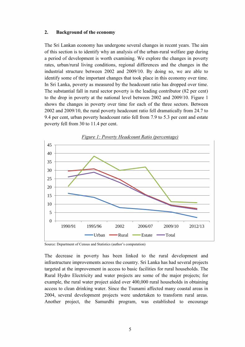
to the drop in poverty at the national level between 2002 and 2009/10. Figure 1

shows the changes in poverty over time for each of the three sectors. Between

2002 and 2009/10, the rural poverty headcount ratio fell dramatically from 24.7 to

9.4 per cent, urban poverty headcount ratio fell from 7.9 to 5.3 per cent and estate

poverty fell from 30 to 11.4 per cent.

Figure 1: Poverty Headcount Ratio (percentage)

Source: Department of Census and Statistics (author’s computation)

The decrease in poverty has been linked to the rural development and

infrastructure improvements across the country. Sri Lanka has had several projects

targeted at the improvement in access to basic facilities for rural households. The

Rural Hydro Electricity and water projects are some of the major projects; for

example, the rural water project aided over 400,000 rural households in obtaining

access to clean drinking water. Since the Tsunami affected many coastal areas in

2004, several development projects were undertaken to transform rural areas.

Another project, the Samurdhi program, was established to encourage

0

5

10

15

20

25

30

35

40

45

1990/91 1995/96 2002 2006/07 2009/10 2012/13

Urban Rural Estate Total

6

participation of the poor, expanding opportunities for self- and wage employment

at rural levels.

Statistics from the Censuses of Population and Housing for 2001 and 2011 show

vast improvements in the access to various facilities such as clean water,

electricity and the major sources of cooking fuel. While this is especially true for

rural and estate areas, it is also the case that urban areas saw improvements. In

2001, 85.3 per cent of urban households had electricity as the main source of

lighting and this rose to 96 per cent in 2011. In the rural sector, 62 per cent of

households had electricity as the major source of lighting in 2001. By 2011, 85 per

cent of the rural households had electricity. The main source of drinking water

used by urban households is piped-born water (77.8 per cent of the households in

2001 and remained quite stagnant even in 2011). For the rural sector, the main

source of drinking water comes from wells; in 2001, 58 per cent of rural

households drank from protected wells and 11.5 per cent drank from unprotected

wells. By 2011, the corresponding figures were 54 per cent and 4.8 per cent. In the

urban sector, households use gas as the main source of cooking fuel and this rose

from 45.3 per cent to 53.7 per cent of the population using it between 2001 and

2011. For rural and estate households, the main source is firewood, but more

households report using gas as the main form of fuel in 2011. As the gap in terms

of access to major household facilities has narrowed in recent years, we observe in

our analysis that the urban-rural welfare gap has also narrowed over time.

In the past few years, road and air transportation recorded significant growth. The

development in the transportation sector (particularly covering rural areas) was

largely seen in the road development, with the expansion of transport services

(both, rail and road). Improvements were made in the road network to ease

passenger and goods transportation. A programme to revitalize roads in rural areas

that commenced in 2004 was able to rehabilitate over 840 kilometres of roads

(Central Bank of Sri Lanka, 2012). This focus on rural infrastructure development

became a priority after the Tsunami which damaged significant areas of the rural

transport sector. This enabled easy movement for individuals between towns and

villages.

The country however has seen persistent differences across regions; the Central,

Sabaragamuwa and Uva provinces (that include a large proportion of plantations)

in particular, still have high levels of poverty. UNDP (2012) argues focus on

making improvements at the regional level is required to prevent inequality from

limiting the development of the economy. Regional differences also explain the

significant variances in urban growth rates, and the diverse levels of urbanization

among districts. Table A2 (refer to Appendix 2) presents the urban population by

district. Uduporuwa (2010) showed that the Western province is the core

urbanized region with the higher number of urban centres and highest percentage

of urbanization. Other provinces however have not achieved significant urban

7

growth. Additionally, the country having recently seen the end of a 30-year war

meant that development in the Northern and Eastern provinces was limited for a

long period of time and skilled labour migrated to urban areas in the Western and

Central provinces for better employment opportunities. This variation in levels of

urbanization across districts and provinces motivates the inclusion of district-level

variables in the analysis.

Having discussed the development of rural areas and regional differences that

persist in Sri Lanka, we now turn to the changes in the industry structure that have

taken place in the period under investigation. As we will observe, several changes

occurred in terms of sectoral contribution to GDP and GDP growth, strengthening

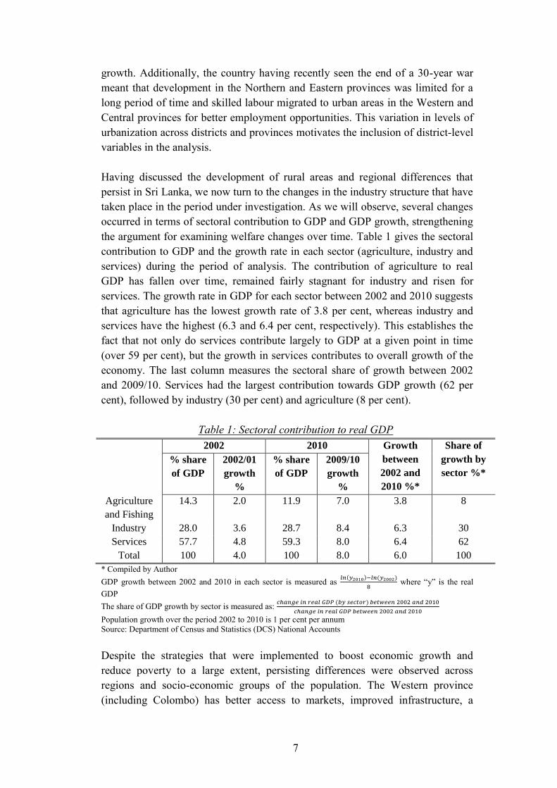
the argument for examining welfare changes over time. Table 1 gives the sectoral

contribution to GDP and the growth rate in each sector (agriculture, industry and

services) during the period of analysis. The contribution of agriculture to real

GDP has fallen over time, remained fairly stagnant for industry and risen for

services. The growth rate in GDP for each sector between 2002 and 2010 suggests

that agriculture has the lowest growth rate of 3.8 per cent, whereas industry and

services have the highest (6.3 and 6.4 per cent, respectively). This establishes the

fact that not only do services contribute largely to GDP at a given point in time

(over 59 per cent), but the growth in services contributes to overall growth of the

economy. The last column measures the sectoral share of growth between 2002

and 2009/10. Services had the largest contribution towards GDP growth (62 per

cent), followed by industry (30 per cent) and agriculture (8 per cent).

Table 1: Sectoral contribution to real GDP

2002 2010 Growth

between

2002 and

2010 %*

Share of

growth by

sector %*

% share

of GDP

2002/01

growth

%

% share

of GDP

2009/10

growth

%

Agriculture

and Fishing

14.3 2.0 11.9 7.0 3.8 8

Industry 28.0 3.6 28.7 8.4 6.3 30

Services 57.7 4.8 59.3 8.0 6.4 62

Total 100 4.0 100 8.0 6.0 100

* Compiled by Author

GDP growth between 2002 and 2010 in each sector is measured as 𝑙𝑛(𝑦2010)−𝑙𝑛(𝑦2002)

8 where “y” is the real

GDP

The share of GDP growth by sector is measured as: 𝑐ℎ𝑎𝑛𝑔𝑒𝑖𝑛𝑟𝑒𝑎𝑙𝐺𝐷𝑃(𝑏𝑦𝑠𝑒𝑐𝑡𝑜𝑟)𝑏𝑒𝑡𝑤𝑒𝑒𝑛2002𝑎𝑛𝑑2010

𝑐ℎ𝑎𝑛𝑔𝑒𝑖𝑛𝑟𝑒𝑎𝑙𝐺𝐷𝑃𝑏𝑒𝑡𝑤𝑒𝑒𝑛2002𝑎𝑛𝑑2010

Population growth over the period 2002 to 2010 is 1 per cent per annum

Source: Department of Census and Statistics (DCS) National Accounts

Despite the strategies that were implemented to boost economic growth and

reduce poverty to a large extent, persisting differences were observed across

regions and socio-economic groups of the population. The Western province

(including Colombo) has better access to markets, improved infrastructure, a

8

greater proportion of educated people, and is dominated by non-agricultural

sectors compared to other provinces. The above findings suggest that the country

has gone through several changes in recent years. This gives rise to the key issue

to be examined in this paper – analysing welfare differences across urban and

rural areas, and how this has changed over time.

3. Literature review

3.1 Theory and findings for other countries

This paper tries to answer the central question of what factors contribute to the

urban-rural welfare gap in Sri Lanka. The motivation for doing so is both

theoretical and methodological.

Theoretically, over the years, two main frameworks have been central to the study

of the urban-rural divide: the view that economic policy is subject to an “urban

bias”, and the Lewis model of surplus rural labour. The concept of an urban bias

was popularized by Lipton (1977) who noted that spatial differences in poverty

between urban and rural areas slows down the development process in poor

countries. Subsequently, the urban-rural gap in welfare and income has been of

concern in development research. The theory of an urban bias stems from the

notion that the government favours urban areas over rural areas because of the

political power of urban dwellers (Knight and Song, 1999). Despite the urban

dwellers being a small proportion of the total population in developing countries,

their influence on government policy is argued to be disproportionate to their

numbers. If the government permits a wage differential favouring urban

employment, rural-urban migration will be in excess of the capacity of urban areas

which in turn gives rise to urban unemployment.

The two-sector model by Lewis (1954) was originally based on the argument that

developing countries have a surplus of unproductive labour in agriculture

primarily in rural areas which can be shifted to the growing manufacturing sector

in urban areas to promote industrialization and sustainable development.

Improving urban areas in this manner was thought to be efficient, but could come

at the cost of national equity. Over time, Lewis’s thinking about the role of

agriculture shifted towards an emphasis on the increase of agricultural

productivity and demand for agricultural goods (Lewis, 1978). This view was

shared by others such as Mellor (1976) and Meier (1989) who identified the

importance of agriculture not only as surplus to support industrialization, but also

to view it as an activity by itself that generates employment, growth and a more

equal distribution of income.

In many developing countries, the urban-rural welfare gap accounts for an

important element of inequality. Vietnam is a case in point and a useful

9

comparator for Sri Lanka given the countries’ structural similarities. In a study on

the Vietnamese urban-rural gap in welfare between 1993 and 2006, Thu Le and

Booth (2014) employed a quantile regression technique and found that Vietnam’s

economic reforms such as the achievement of macroeconomic stability and the

transition from a centrally-planned economy to a market economy in 1986,

enabled households in urban areas to reap the benefits of the reforms (via higher

returns to education) more than households in rural areas. Vietnam, like Sri Lanka

experienced exceptional growth, but a rising urban-rural gap in welfare. However,

since 2002, the urban-rural gap started to decline due to the development and

industrialisation of rural areas. During the latter period, the urban-rural gap fell

during a period of high growth bringing the rural households closer to urban

households in terms of welfare.

Understanding the underlying factors affecting the urban-rural welfare gap is

central to this paper. The growth of certain industries, education and other

household characteristics have been identified in the literature as potential

contributors to the gap in welfare between urban and rural households. Thu Le and

Booth (2014) applied the Blinder-Oaxaca decomposition to the unconditional

quantile regression which identified the crucial role played by remittances and the

loosening of government controls allowing rural migrants to access urban

facilities such as education, health insurance and owning a house. Domestic

remittances became significant in improving rural household expenditure

especially for the rural poor.

The impact of education and occupation choices on the falling urban-rural

differences in wages was studied by Hnatkovska and Lahiri (2013) in the context

of India between 1983 and 2010. Their findings suggest that almost 40 per cent of

the wage convergence observed between urban and rural India was explained by

converging individual characteristics such as education and occupation choices.

Himaz and Aturupane (2011) applied a quantile regression to identify the

importance of education on household welfare in Sri Lanka using five cross-

section datasets between 1985 and 2006. Their paper found that people in higher

quantiles who have greater consumption expenditure are more likely to have

higher levels of education and better skills that complement education, thus

enabling them to earn higher returns to education. The findings also indicated that

residing in a rural area had a negative impact on the returns to education compared

to residing in an urban area, especially at the top end of the welfare distribution.

Finally, Sicular et al. (2007) examined the urban-rural gap in China and found that

with better infrastructure and employment opportunities, people in rural areas can

easily move to urban areas for employment. The paper noted that the exclusion of

migrants and ignoring spatial price differentials across regions led to an over-

estimation of the urban-rural gap.

10

3.2 Methods used in the literature

Measuring inequality is not straightforward. Many methods have been advanced

to try to decompose inequality in order to better understand its causes. The Gini

and Theil coefficients, for example, have been used often to decompose inequality

into a within- and between-group component – how much of the inequality is due

to inter-group effects and how much of it is due to intra-group effects. Although

this helps understand the sources of inequality growth/decline, the between versus

within decomposition does not identify the factors affecting the welfare or income

distributions.

Methods allowing the entire conditional distribution (rather than just the

conditional variance) to be estimated were introduced (such as Machado and

Mata, 2005). This technique creates a counterfactual distribution for one of the

two groups (rural, in this case) and compares it to the actual distributions in order

to separate the urban-rural differences in welfare into two components – the first

is the contribution of the differences in urban-rural household characteristics to

the welfare gap (covariate effect; for example, the different education levels

between the areas) and the second is how the differences in urban-rural returns to

those characteristics contribute to the welfare gap (returns effect; for example, the

returns to education).

The decomposition gives a better understanding of how the contributions of

characteristics and returns to characteristics have changed over time in affecting

the urban-rural welfare gap. Nguyen et al. (2007) implemented this method in

Vietnam in the period of rapid growth and rising inequality, noting that

differences in covariates explain most of the urban-rural expenditure gap at lower

quantiles; but for the rest of the expenditure distribution, the gap was primarily

due to urban-rural differences in the returns to covariates. However, the drawback

of this approach is that the decomposition is not detailed enough to compute the

sub-components of the covariate effect; that is, to identify the specific sources that

give rise to the differences in covariate distributions between the urban and rural

areas.

Firpo et al. (2009) introduced a new technique which is an extension of the

Machado-Mata (2005) decomposition identifying the detailed components of

both, the returns and covariate effects. This is done through the estimation of (re-

centred) influence function (RIF, hereafter) regressions. In this context, the RIF

can be regarded as an unconditional quantile regression. Instead of using the

traditional conditional quantile regression, this technique used the unconditional

quantile regression. Koenker and Bassett (1978) introduced the (conditional)

quantile regression technique. This method estimates the effects of each

explanatory variable on the entire distribution of expenditure. However, it is

restrictive since a change in the distribution of covariates could change the

11

interpretation of the estimated coefficients (Firpo et al., 2009). Fortin (2008) and

Firpo et al. (2009) estimated the effect of union status on log wages of men in the

United States and found large differences between the results using the

conditional and unconditional quantile regressions.

The estimates from the unconditional quantile regressions suggested that

unionization progressively increases wages at the bottom end of the distribution,

and reduces wages at the top end of the distribution which precisely explained the

U-shaped changes observed in the actual wage data. The conditional regression

results, in contrast, suggest that unionization has a positive yet monotonically

declining effect on wages without taking into account the observed changing

pattern of the wage distribution. It is clear that the two different methods interpret

results differently. Therefore, for the purpose of this study where it is important to

understand how each household characteristic contributes to the welfare gap, an

unconditional quantile regression is suitable.

In order to analyse the welfare gap between urban and rural areas, the

conventional methodology proposed by Blinder (1973) and Oaxaca (1973) can be

implemented. This standard decomposition stems from the notion that differences

in expenditure between urban and rural households may arise from three possible

sources – differences in endowments, differences in returns to endowments, and

differences in unobservable characteristics. However, the Blinder-Oaxaca

decomposition technique is carried out at the mean of the expenditure distribution.

For the analysis of the urban-rural gap, it is important to examine the entire

distribution. Firpo et al. (2009) apply a variant of the Blinder-Oaxaca

decomposition to the estimates obtained from the unconditional quantile

regression. This method was used by Thu Le and Booth (2014) in their study of

the urban-rural welfare gap in Vietnam and will be used in this paper.

This paper contributes to the existing literature in two ways. Firstly, it explores the

welfare gap between urban and rural households in Sri Lanka during a period of

rapid growth. This has not been examined to date - Himaz and Aturupane (2011)

observed the effect of education on household welfare between 1985 and 2006 in

Sri Lanka, however urban and rural households were pooled together. This paper

extends the analysis to 2009/10 and isolates urban and rural households to identify

welfare differences across the expenditure distribution and over time. Secondly

from a methodological viewpoint, this paper adds a new dimension with the use of

an unconditional quantile regression as opposed to the conventional quantile

regression technique. The use of a decomposition technique allows a further

examination of the urban-rural gap to identify which factors were crucial in

changing the welfare gap over time and across the expenditure distribution. It thus

extends the existing literature with a detailed analysis of the contributing factors to

urban-rural welfare gaps in Sri Lanka between 2002 and 2009/10. The next

section will explain the data used in the paper.

12

4. Data

4.1 Data and sample

The Household Income and Expenditure Surveys (HIES) of 2002 and 2009/10 are

used in this study to cover the period of dramatic change in Sri Lanka. Data was

collected in twelve consecutive monthly rounds in order to capture seasonal

variations in income and consumption patterns. The 2002 survey was conducted

from January 2002 through December 2002 and includes 16,920 households, and

the 2009/10 survey was conducted from July 2009 through June 2010 and

includes 17,182 households. For comparability, only provinces/districts included

in both waves are included in the analysis – 17 out of the 25 districts in the

country have been surveyed in both years.

In the HIES carried out in 2002, the Northern and Eastern provinces were

excluded because of the ongoing war in these areas. By 2009/10, data collection

commenced in 5 additional districts in the aforementioned provinces. However,

the districts were not surveyed for the entire 12 months - the Vavuniya district in

the Northern province and the entire Eastern province were surveyed for 10 out of

the 12 months whereas the Jaffna district in the Northern province was surveyed

for 7 months. The remaining 3 districts in the country were left out of the 2009/10

survey due to ongoing resettlement activities.

The excluded districts include 2,776 households in the 2009/10 survey data, 40

per cent of whom are from urban areas. The descriptive statistics for the excluded

districts in 2009/10 suggest that these districts have lower real expenditure per

capita at every quantile, on average in comparison to the rest of the country –

particularly at higher quantiles where large urban-rural differences in expenditure

are seen). Households are smaller and these districts are predominantly rural (see

Appendix 2). Descriptive statistics on these excluded districts obtained from the

HIES 2009/10 are discussed in Appendix 1.

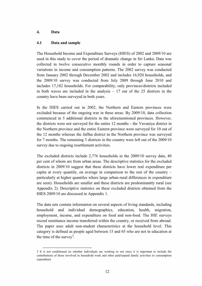
The data sets contain information on several aspects of living standards, including

household and individual demographics, education, health, migration,

employment, income, and expenditure on food and non-food. The HIE surveys

record remittance income transferred within the country, or received from abroad.

The paper uses adult non-student characteristics at the household level. This

category is defined as people aged between 15 and 65 who are not in education at

the time of the survey3.

3 It is not conditioned on whether individuals are working or not since it is important to include the

contributions of those involved in household work and other paid/unpaid family activities to consumption

expenditure

13

To compare the differences across urban and rural living standards, monthly

household per capita expenditure was used – at 2002 prices. For the purpose of

this study, the inclusion of private consumption (such as home-produced food) is

an important indicator of economic welfare. Consumption data also reduces the

issue of variability that income may have across the survey period (Deaton, 1997).

Total household expenditure was calculated as the sum of expenditure on food and

non-food items. Food expenditure includes the expenditure on purchased products

as well as home-produced items. For home-produced items, the total quantity

consumed was multiplied by the unit value if it were purchased in the market4.

Non-food expenditure includes expenditure on housing5, education, health,

clothing, entertainment, communication, personal health care, household goods,

transportation and vehicle maintenance.

Once we obtain total monthly expenditure (on food and non-food items) for a

household, we then adjust for spatial variations in prices across the 17 districts.

The price indices for both years (2002 and 2009/10) are presented in Appendix 2

(Table A2). According to the Department of Census and Statistics, Laspeyres

price indices were calculated using unit prices of the typical consumer food basket

for each district. Note that the price indices are observed at a given point in time at

the district level, and are updated over the survey periods. By adjusting monthly

expenditure to account for spatial price differences, we obtain expenditure values

that are free from commodity price differences across districts. We are unable to

disaggregate the indices further than district-level in order to observe price

variations across urban and rural areas. However as shown in Table A2, the

districts are either predominantly urban or rural – thus, the spatial price indices

capture a part of the urban-rural price differences.

Next, the monthly household expenditure is converted into real terms. This is

useful for the comparison of expenditure over time. In order to do this, household

expenditure is divided by the Consumer Price Index (base year is 2002). Thus, the

expenditure values are at 2002 prices. Finally to obtain per-capita values, the real

expenditure is divided by the number of members in the household. The main

variable of the analysis is obtained - real per capita expenditure (RPCE). In this

manner, we are able to account for spatial price variations across regions, which

Sicular et al. (2007) noted to be important when estimating the urban-rural gap.

We identify a caveat in the analysis as the data does not include information on

migration – we are unable to identify individuals who may have migrated from

4 The HIES survey report explains that unit values were estimated according to the market value, including

homegrown food or items received free of charge. This information is initially recorded in a separate form by

the respondent (under the guidance of the enumerator during the visit to the household). It is later edited if

necessary and recorded in the survey schedule by the enumerator.

5 Rent values were imputed for those living in their own house

14

rural to urban areas due to improved infrastructure, for example. However, we

attempt to deal with this issue by including controls for remittance flows received

from abroad or within the country. Workers’ remittances have become an

increasingly attractive source of financing over the past three decades in Sri

Lanka. In 2010, remittances accounted for 8.3 per cent of GDP (World Banka

data), which is high compared to countries of broadly equal size and other Asian

countries in 2005 (Lueth and Ruiz-Arranz, 2007). This finding was confirmed by

Himaz and Aturupane (2011) – the paper stated that the remittance flows across

the country and from foreign countries increased by nearly eight-fold in real terms

over the 20 years that were analysed – being 3 per cent of consumption in 1985

and 13 per cent in 2006.

The next section explores descriptive statistics in order to understand some of the

key movements across urban and rural sectors, over time, and across rich and poor

households.

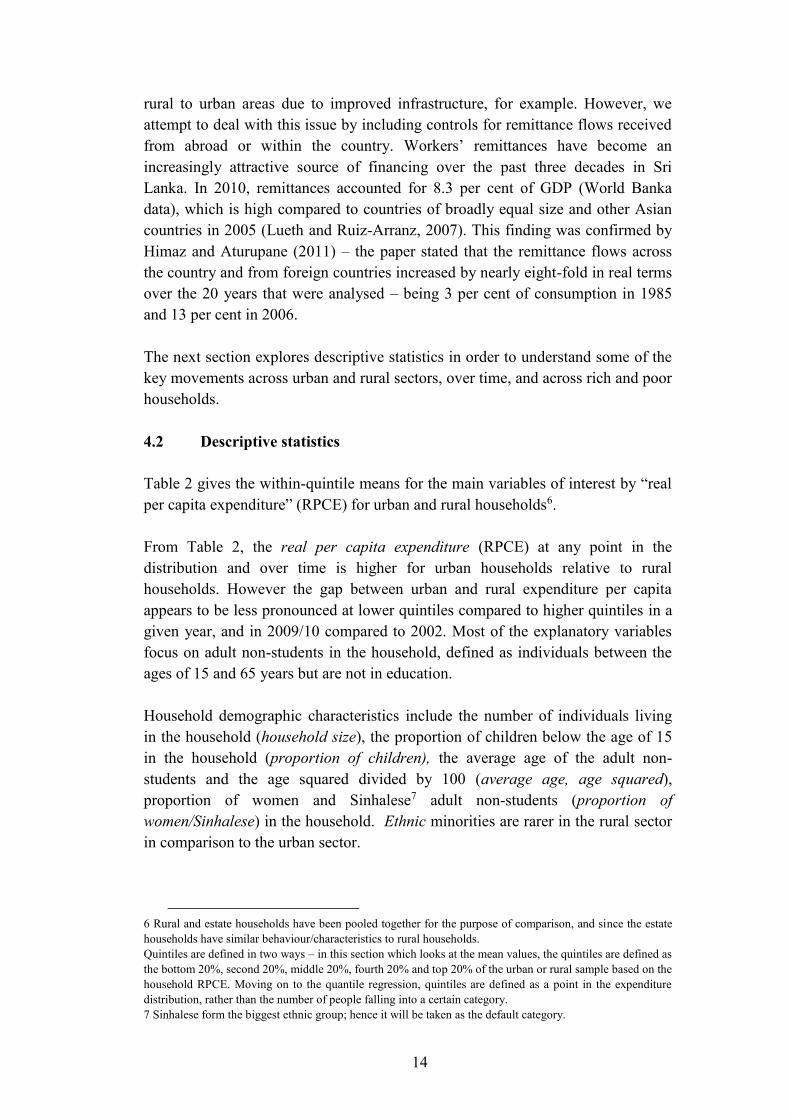
4.2 Descriptive statistics

Table 2 gives the within-quintile means for the main variables of interest by “real

per capita expenditure” (RPCE) for urban and rural households6.

From Table 2, the real per capita expenditure (RPCE) at any point in the

distribution and over time is higher for urban households relative to rural

households. However the gap between urban and rural expenditure per capita

appears to be less pronounced at lower quintiles compared to higher quintiles in a

given year, and in 2009/10 compared to 2002. Most of the explanatory variables

focus on adult non-students in the household, defined as individuals between the

ages of 15 and 65 years but are not in education.

Household demographic characteristics include the number of individuals living

in the household (household size), the proportion of children below the age of 15

in the household (proportion of children), the average age of the adult non-

students and the age squared divided by 100 (average age, age squared),

proportion of women and Sinhalese7 adult non-students (proportion of

women/Sinhalese) in the household. Ethnic minorities are rarer in the rural sector

in comparison to the urban sector.

6 Rural and estate households have been pooled together for the purpose of comparison, and since the estate

households have similar behaviour/characteristics to rural households.

Quintiles are defined in two ways – in this section which looks at the mean values, the quintiles are defined as

the bottom 20%, second 20%, middle 20%, fourth 20% and top 20% of the urban or rural sample based on the

household RPCE. Moving on to the quantile regression, quintiles are defined as a point in the expenditure

distribution, rather than the number of people falling into a certain category.

7 Sinhalese form the biggest ethnic group; hence it will be taken as the default category.

15

Household size has a negative relationship with per capita expenditure implying

that larger households are poorer, on average. However, due to size economies

this could be biased upwards. Poorer households spend a greater proportion of

their income on rival goods such as food. Yet their consumption of certain items

such as clothing, housing, water taps, etc. are shared among several members in

the household – such bulk purchases suggest that the cost per person is lower

(with a given standard of living) when more individuals live together, rather than

separately. A common belief is that larger households tend to be poorer. However,

a paper by Lanjouw and Ravallion (1995) discuss that this relationship between

household size and poverty/expenditure may vanish at a certain point due to size

economies in consumption. The paper employed a method whereby the total

expenditure is divided by the household size raised to a power less than one (given

a value of θ). This value is known as the size elasticity. As the value of θ

decreases, consumption expenditure and household size become statistically

independent. At values of θ larger than the threshold value, bigger households

tend to have lower expenditure. For Sri Lanka, the value of θ at which point the

household size and expenditure begin to have the negative relationship is at 0.3 for

urban households and 0.6 for rural households. The low value of θ for urban

households suggests that there is a negative relationship between household size

and expenditure; whereas for rural households, the correlation between poverty

and household size may vanish when there are size economies in consumption.

Human capital is measured by the average number of years of education acquired

by the adult non-students (education). The average education level increases

across quintiles as expected for urban and rural sectors, and at any given point, it

is higher for urban households than for rural households. Dummy variables are

used to identify whether or not the household received remittance income from

within Sri Lanka (local remit) or from abroad (foreign remit) during the year. At a

given point in time, a greater proportion of rural households receive local

remittance income whereas a greater proportion of urban households receive

foreign remittance income. Both, foreign and local remittance transfers have

increased over time – specifically foreign remittance income received by urban

households and local remittance income received by rural households.

The type of employment (wage, self-employed or not employed) is accounted for

by the variables that measure the proportion of adult non-students in the

household who are working in wage employment, self-employment or are not in

the labour force8. We use the reported income by individuals to distinguish

between the wage employees and self-employed. Individuals with more than one

source of income were distinguished as being either wage/self-employed by

looking at the source which yielded the highest income. Looking at the descriptive

8 This category is for the adult non-students who are unemployed, retired/disabled and stay-at-home parents

during the sample period.

16

statistics, there are a greater proportion of adults in some form of employment in

the rural sector compared to the urban sector; this is true at any given point in the

expenditure distribution and for both years. Both, being in wage and self-

employment have a positive relationship with per capita expenditure across the

distribution. Over time, the proportion of adults in urban areas working in self-

employment has risen for the top end of the distribution and the proportion of

adults in wage employment has fallen. In rural areas, the proportion of adults in

wage employment has fallen over time whereas the proportion in self-employment

has risen marginally.

Additional variables are used to account for the sector (agriculture, manufacturing

or services) of the working adult non-students (that is, those in wage and self-

employment) shown as proportions in the relevant form of employment (for

example, the proportion of working adult non-students in the services industry).

Per capita expenditure appears to have a negative relationship with agriculture

employment and a positive relationship with service employment in both, urban

and rural areas. Further, there is a larger proportion of agricultural workers and a

smaller proportion of service sector workers in rural areas compared to urban

areas. These findings are what would be expected in a developing country

(Nguyen et al, 2007; Thu Le and Booth, 2014).

Having observed various changes in household characteristics, three interesting

questions emerge. Firstly, what factors affect the urban and rural expenditure per

capita, and how has it changed over time? Secondly, to what extent is household

expenditure per capita determined by the observed productivity-related

characteristics (as mentioned in this section) in urban and rural areas? Finally,

how much of the urban-rural expenditure differential can be contributable to

urban-rural differences in average characteristics, and how much of the

expenditure differential can be contributable to the difference in returns to those

characteristics and other factors which are not captured in the model? The paper

proceeds as follows. Section 5 will look at the determinants of urban and rural

expenditure per capita across the expenditure distribution in both years; in section

6, the results obtained will be used in a decomposition that will enable isolation of

the factors that give rise to the urban-rural gap in expenditure.

17

Table 2: Within-quintile means of variables by log RPCE for urban and rural households

2002 Urban (3,240 households) Rural (13,680 households)

Variable 1st 2nd 3rd 4th 5th 1st 2nd 3rd 4th 5th

RPCE (at 2002 prices) 1497 2420 3506 5315 11639 1052 1562 2096 2945 6648

Household size 5.67 5.09 4.54 4.17 3.62 5.09 4.59 4.22 3.92 3.67

Children (proportion) 0.25 0.20 0.17 0.16 0.12 0.26 0.21 0.19 0.17 0.15

Average age 30 33 35 37 41 31 33 34 36 38

Education 4.72 6.97 7.67 8.85 10.08 4.64 5.50 6.04 6.91 8.63

Women (prop.) 0.50 0.50 0.52 0.51 0.52 0.49 0.49 0.50 0.50 0.50

Sinhalese (prop.) 0.56 0.65 0.71 0.74 0.78 0.79 0.80 0.81 0.87 0.92

Local remit (0,1) 0.04 0.03 0.05 0.05 0.05 0.06 0.06 0.05 0.06 0.05

Foreign remit (0,1)

0.05 0.06 0.10 0.07 0.08 0.03 0.04 0.04 0.05 0.05

Wage (prop.) 0.24 0.26 0.27 0.31 0.37 0.26 0.28 0.29 0.27 0.33

Self-employed (prop.) 0.08 0.11 0.11 0.11 0.11 0.11 0.14 0.16 0.18 0.17

Not employed (prop.) 0.68 0.63 0.62 0.58 0.52 0.63 0.58 0.55 0.55 0.50

Of the employed:

Agriculture (prop.) 0.09 0.06 0.06 0.05 0.02 0.49 0.47 0.41 0.32 0.20

Manufacture (prop.) 0.28 0.21 0.20 0.22 0.18 0.19 0.19 0.20 0.21 0.19

Services (prop.) 0.63 0.73 0.74 0.73 0.80 0.32 0.34 0.39 0.47 0.61

18

The key variable of interest is “real per capita expenditure”, calculated in Sri Lankan rupees at 2002 prices (1 USD ≈ 146 LKR). The explanatory variables are computed using adult non-

student characteristics. Education is measured as the average years of education obtained by adult non-students. The employment variables give the proportion of adult non-students in

wage or self-employment, or not a part of the work force (not employed). The category of not being in employment is the adult non-students who are unemployed, retired/disabled and stay-

at-home parents during the sample period. For the wage and self-employed adults, the sectoral variables capture the proportion of wage/self-employed adults in agriculture, manufacturing

or the services sector

2009/10 Urban (4,192 households) Rural (12,990 households)


RPCE (at 2002 prices) 1788 2817 3884 5465 12576 1453 2171 2876 3931 8060

Household size 5.57 4.72 4.36 4.05 3.49 5.01 4.44 4.16 3.93 3.55


Average age 32 34 36 39 43 32 34 37 37 40

Education 5.78 6.72 7.50 8.41 9.72 4.72 5.63 6.36 7.21 8.76

Women (prop.) 0.53 0.53 0.54 0.53 0.53 0.50 0.51 0.52 0.52 0.52

Sinhalese (prop.) 0.58 0.64 0.69 0.72 0.76 0.66 0.72 0.78 0.84 0.89

Local remit (0,1) 0.05 0.04 0.05 0.05 0.02 0.11 0.09 0.08 0.08 0.07

Foreign remit (0,1)

0.08 0.08 0.09 0.10 0.12 0.06 0.04 0.06 0.05 0.08

Wage (prop.) 0.24 0.24 0.26 0.28 0.31 0.24 0.26 0.26 0.25 0.30



Of the employed:



Services (prop.) 0.60 0.65 0.67 0.71 0.77 0.29 0.34 0.38 0.49 0.61

19

5. Determinants of urban and rural per capita expenditure

5.1 Method

The paper focuses on the link between household characteristics and real per

capita expenditure (RPCE) across urban and rural areas. As per capita expenditure

varies across the distribution in both, urban and rural areas, there is a need to

examine the entire distribution of expenditure rather than simply focussing on the

mean (as an Ordinary Least Squares estimation would do). For this purpose, a

quantile regression is more suitable.

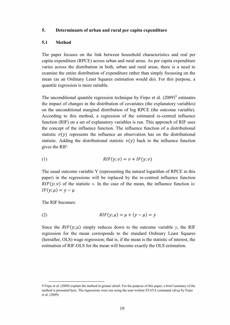
The unconditional quantile regression technique by Firpo et al. (2009)9 estimates

the impact of changes in the distribution of covariates (the explanatory variables)

on the unconditional marginal distribution of log RPCE (the outcome variable).

According to this method, a regression of the estimated re-centred influence

function (RIF) on a set of explanatory variables is run. This approach of RIF uses

the concept of the influence function. The influence function of a distributional

statistic 𝑣(𝑦) represents the influence an observation has on the distributional

statistic. Adding the distributional statistic 𝑣(𝑦) back to the influence function

gives the RIF:

(1) 𝑅𝐼𝐹(𝑦; 𝑣) = 𝑣 + 𝐼𝐹(𝑦; 𝑣)

The usual outcome variable Y (representing the natural logarithm of RPCE in this

paper) in the regressions will be replaced by the re-centred influence function

𝑅𝐼𝐹(𝑦; 𝑣) of the statistic v. In the case of the mean, the influence function is:

𝐼𝐹(𝑦; 𝜇) = 𝑦 − 𝜇

The RIF becomes:

(2) 𝑅𝐼𝐹(𝑦; 𝜇) = 𝜇 + (𝑦 − 𝜇) = 𝑦

Since the 𝑅𝐼𝐹(𝑦; 𝜇) simply reduces down to the outcome variable y, the RIF

regression for the mean corresponds to the standard Ordinary Least Squares

(hereafter, OLS) wage regression; that is, if the mean is the statistic of interest, the

estimation of RIF-OLS for the mean will become exactly the OLS estimation.

9 Firpo et al. (2009) explain the method in greater detail. For the purpose of this paper, a brief summary of the

method is presented here. The regressions were run using the user-written STATA command rifreg by Firpo

et al. (2009)

20

Similarly, the influence function can be computed for various quantiles of the

expenditure distribution. At the quantile𝜃, the RIF will be:

(3) 𝑅𝐼𝐹(𝑦; 𝑞𝜃) = 𝑞𝜃 + 𝐼𝐹(𝑌; 𝑞𝜃) = 𝑞𝜃 +𝜃−1{𝑦≤𝑞𝜃}

𝑓𝑦(𝑞𝜃)

This new method used by Firpo et al. (2009) that estimates the unconditional

quantile regression can be done through one of the three techniques: Ordinary

Least Squares (namely, RIF-OLS), logistic (namely, RIF-logit) or non-parametric

(namely, RIF-nonparametric). This paper uses RIF-OLS for simplicity10. The RIF

estimations are then included in the regressions instead of log RPCE which will be

explored in the next section.

5.2 Model specifications

To understand the relationship between the natural log of real per capita

expenditure (RPCE) and various household characteristics, especially how they

differ across urban and rural areas over the entire distribution of log RPCE,

quantile regressions of the following form will be estimated:

(4) 𝑌𝑖 = 𝛼 + 𝛽𝑋𝑖 + 𝛾𝑈𝑖 + 𝛿𝑈𝑖. 𝑋𝑖 + 휀𝑖

where “Y” is the dependent variable – log RPCE of household i, 𝑈𝑖 is the urban

dummy, 𝑋𝑖is the vector of explanatory variables for the household (excluding

“u”), and 𝑈𝑖 . 𝑋𝑖 is the interaction between the urban dummy and explanatory

variables. The vector of coefficients 𝛽 represents the returns to characteristics; 𝛾

and 𝛿 coefficients are the respective intercept and slope differential for the urban

dummy variable. The explanatory variables (𝑋𝑖) include education, demographic,

employment and geographical characteristics of the household of adult non-

students. To control for regional differences, dummies for regions will be

included. The way each characteristic is captured was explained in Section 4.2.

This paper analyses the urban-rural gap in welfare in two stages. Firstly, the

urban and rural households will be analysed separately to observe the factors

affecting real per capita expenditure for both these sectors. The second part will be

a decomposition of the urban-rural gap in the expenditure distribution. The total

urban-rural gap can be disaggregated into two components. The first is the

contribution of urban-rural differences in the distributions of covariates such as

education to the urban-rural gap (covariate effect). The second component arises

from the differences in the distributions of returns to these covariates (returns

effect). To decompose the urban-rural gap across the log RPCE distribution and

isolate the two effects, the results obtained from the quantile regression are

10 Firpo et al. (2009) obtained similar results using all three estimation techniques

21

applied to a Blinder-Oaxaca decomposition. This technique will be discussed in

greater detail in Section 6 after estimating the quantile regressions to identify the

factors affecting urban and rural real per capita expenditure across the distribution.

5.3 Results

In this section, the household level determinants of real per capita expenditure are

analysed in urban and rural areas for both sample periods – 2002 and 2009/10. We

start by testing whether the urban and rural samples need to be analysed in

isolation. In order to do this, quantile regressions were estimated for the pooled

sample (urban and rural) to test and confirm that there are significant differences

in per capita expenditure across these two areas which are worth analysing further.

The two tests that were conducted will be explained in detail below.

As noted from the descriptive statistics in Section 4.2, a “raw” gap in per capita

expenditure was identified between urban and rural households. A regression

allows us to control for several household factors and identify the “pure” gap

which may or may not exist after controlling for other factors. The first test

employs a model of Equation 4 that includes the intercept, urban dummy and the

explanatory variables run at the mean using OLS and at selected quantiles using

the unconditional quantile regression for the entire sample. The quantile

regression allows for returns to vary with the households’ positions in the

distribution that are not accounted for by a mean regression. The inclusion of an

urban dummy in a regression identifies the urban-rural gap in per capita

expenditure as the “pure gap” after controlling for other factors.

Figure 2 plots the coefficients on the urban dummy variables in a bar chart11. A

detailed table of estimation results including household characteristics is given in

the Appendix (Table A3). The coefficients are positive and significant suggesting

that, other things being equal, an urban household has higher per capita

expenditure than a comparable rural household. Between 2002 and 2009/10, the

urban-rural gap has fallen; the coefficients on the urban dummies are lower in

2009/10 compared to the coefficients in 2002. In 2002, urban households spent 23

per cent more than their rural counterparts at the median. By 2009/10 this has

dropped; urban households spent 14 per cent more than their rural counterparts (at

the median).

Looking at the entire distribution at a given point in time, the coefficients on the

urban dummies are increasing monotonically up the expenditure distribution

which suggests that the urban-rural differences in per capita expenditure are

higher for households at the top end of the distribution. This is true for 2002 as

well as 2009/10. In 2002 for the 25th quantile, households in urban areas spent 16

per cent more than their rural counterparts. At the other end of the distribution at

11 Here we interpret the coefficient as (exp(β)-1) which is the exponential of the coefficient (β).

22

the 75th quantile, households in urban areas spent almost 50 per cent more than

their rural counterparts. By 2009/10, the coefficients on the urban dummy

variables are much lower at any given quantile, but are rising (from a 10 per cent

expenditure differential at the bottom end to a 22 per cent differential at the top

end of the distribution). This suggests that the per capita expenditure differences

between urban and rural areas are larger for richer households.

Figure 2: Quantile regression for full sample (coefficients on urban dummies)

Having analysed the movements of the urban dummy across the distribution and

over time, the above test confirms that there are indeed significant urban-rural

differences in per capita expenditure at the 1 per cent significance level. In the

next test we estimate Equation 4, including all variables being interacted with the

urban dummy variable. The estimation results from this specification are given in

the Appendix (Table A4). An F-test was carried out to test the hypothesis that all

the coefficients of the interaction terms (between the urban dummy and the

observables) are equal to zero. For both survey years, the test rejects the null

hypothesis12 – therefore, there are significant differences in the returns to

household characteristics between urban and rural areas. The specification

includes the intercept, urban dummy, the explanatory variables and the interaction

terms of the urban dummy with the set of explanatory variables at the mean using

OLS and at selected quantiles using the unconditional quantile regression

framework. The interaction terms where the urban dummy is interacted with each

explanatory variable identify urban-rural differences in the coefficients. Therefore,

12 The null hypothesis can be rejected at the 1 per cent significance level at the mean and the 25th, 50th and

75th quantiles. The P-value is 0.00 in all cases

0.00

0.10

0.20

0.30

0.40

0.50

0.60

Q25th Q50th Q75th OLS

Coef

fici

ent on

th

e U

rban

du

mm

y

2002 2009/10

23

we can directly test whether the returns to household characteristics (given by the

β terms in equation 4) differ between the two sectors rather than solely focussing

on the household characteristics (given by the X terms in equation 4). This has

been used by Nguyen et al. (2007) and Thu Le and Booth (2014) in the case of

Vietnam and is a useful way of identifying the most important factors affecting

the urban-rural gap13. The coefficients on the urban dummy measure the urban-

rural gap that is not explained by the covariates in the regressions. We note the

insignificance of the urban dummy in most of the quantiles for both years (with

the exception of the means in both years where the urban coefficient is significant

at the 1 per cent level).

Having confirmed that urban-rural differences do exist even after controlling for

household characteristics and that there are significant differences in returns to

household characteristics between urban and rural areas, we move to the main part

of the analysis. This involves examining the determinants of per capita

expenditure at selected quantiles using the unconditional quantile regression for

urban and rural sectors separately. The estimation results are reported in Tables 3

and 4.

13 The assumption made about the distribution of the error terms is different in comparison to using separate

urban and rural samples – the use of interaction terms in a pooled sample assumes that the error terms are

drawn out from the same error distribution. However, if the sample is split between urban and rural

households, the error terms are different since they are drawn out from two separate samples.

24

Table 3: Determinants of urban household expenditure per capita at the mean and selected quantiles in 2002 and 2009/10

Variables Q25th Q50th Q75th OLS

2002 2009/10 2002 2009/10 2002 2009/10 2002 2009/10

Personal characteristics (average of non-student adults):

Female -0.017

(-0.27)

-0.001

(-0.22)

0.040

(0.55)

-0.087

(-1.63)

-0.150*

(-1.84)

-0.055

(-0.82)

-0.068

(-1.39)

-0.064

(-1.57)

Sinhalese 0.138***

(4.22)

0.058**

(2.06)

0.065*

(1.85)

0.057**

(2.19)

-0.019

(-0.52)

0.008

(0.27)

0.067***

(2.77)

0.023

(1.16)

Average age -0.038***

(-7.32)

-0.023***

(-5.97)

-0.059***

(-10.25)

-0.028***

(-6.87)

-0.047***

(-7.34)

-0.039***

(-7.94)

-0.048***

(-12.43)

0.030***

(-10.01)

Average age2 0.045***

(7.69)

0.023***

(5.18)

0.077***

(11.51)

0.029***

(6.44)

0.067***

(8.88)

0.042***

(7.23)

0.064***

(14.02)

0.031***

(9.14)

Education 0.116***

(19.97)

0.090***

(19.77)

0.120***

(24.98)

0.109***

(25.93)

0.137***

(21.48)

0.125***

(23.99)

0.113***

(31.86)

0.107***

(31.06)

Job type (average of non-student adults; default – unemployed/not employed):

Wage 0.029

(0.44)

0.052

(0.92)

0.371***

(4.72)

0.132**

(2.25)

0.465***

(5.15)

0.228***

(3.05)

0.389***

(6.84)

0.121***

(2.68)

Self-employed 0.383***

(4.63)

0.370***

(5.98)

0.452***

(4.32)

0.378***

(5.17)

0.544***

(4.72)

0.397***

(4.18)

0.516***

(7.50)

0.353***

(6.45)

Job sector (average of non-student adults; default - agriculture):

Manufacturing -0.076

(-1.32)

-0.013

(-0.35)

0.030

(0.59)

-0.052

(-1.46)

0.057

(1.11)

-0.069*

(-1.74)

-0.017

(-0.48)

-0.049*

(-1.87)

Services 0.140***

(2.89)

0.152***

(3.91)

0.171***

(3.31)

0.169***

(4.22)

0.180***

(3.50)

0.181***

(5.77)

0.161***

(4.53)

0.166***

(5.03)

Other demographic characteristics:

Children

(proportion)

0.164*

(1.68)

0.229***

(2.93)

0.592***

(5.76)

0.249***

(3.26)

0.632***

(5.94)

0.279***

(3.23)

0.424***

(6.12)

0.234***

(4.13)

25

Refer to Table A8 for a detailed explanation of how the variables were constructed; t statistics in parentheses; * p < 0.1, ** p < 0.05, *** p < 0.01; the standard errors are bootstrapped with 500

replications

Household size

(log)

-0.381***

(-12.09)

-0.462***

(-16.97)

-0.497***

(-14.61)

-0.478***

(-18.15)

-0.468***

(-12.67)

-0.498***

(-14.74)

-0.457***

(-18.89)

-0.487***

(-22.99)

Foreign remit

(0,1)

0.308***

(6.52)

0.240***

(6.60)

0.264***

(4.46)

0.240***

(6.39)

0.209***

(3.35)

0.223***

(4.71)

0.237***

(6.03)

0.241***

(8.05)

Local remit

(0,1)

0.215***

(3.47)

0.056

(0.99)

0.231***

(3.25)

0.033

(0.56)

0.252***

(3.17)

-0.085

(-1.36)

0.222***

(4.63)

-0.028

(-0.68)

Regions (default – Sabaragamuwa):

Western 0.301***

(4.54)

0.325***

(5.24)

0.305***

(4.64)

0.291***

(5.47)

0.410***

(6.91)

0.339***

(6.02)

0.325***

(7.17)

0.307***

(7.31)

Central 0.174***

(2.38)

0.234***

(3.28)

0.208***

(2.83)

0.154**

(2.43)

0.356***

(5.14)

0.162**

(2.45)

0.241***

(4.75)

0.157***

(3.22)

Southern 0.027

(0.40)

0.323***

(4.88)

0.102

(1.38)

0.232***

(4.17)

0.216***

(3.20)

0.286***

(4.81)

0.104**

(2.03)

0.258***

(5.92)

North West 0.139

(1.58)

0.240***

(3.21)

0.174*

(1.92)

0.220***

(3.39)

0.273***

(3.31)

0.185**

(2.57)

0.204***

(3.47)

0.193***

(3.69)

North Central 0.201**

(2.13)

0.229***

(2.68)

0.084

(0.84)

0.235***

(3.00)

0.052

(0.53)

0.268***

(2.97)

0.103

(1.49)

0.249***

(4.02)

Uva 0.045

(0.46)

0.234**

(2.55)

0.218**

(2.18)

0.170**

(2.08)

0.414***

(3.78)

0.102

(1.21)

0.141**

(2.05)

0.195***

(3.02)

Constant 7.433***

(58.63)

7.815***

(74.38)

7.897***

(57.80)

8.207***

(82.06)

8.194***

(56.56)

8.731***

(73.95)

7.920***

(84.97)

8.326***

(109.72)

Number of

observations

3,240 4,192 3,240 4,192 3,240 4,192 3,240 4,192

R-squared 0.24 0.19 0.29 0.25 0.25 0.23 0.43 0.36

26

Table 4: Determinants of rural household expenditure per capita at the mean and selected quantiles in 2002 and 2009/10


2002 2009/10 2002 2009/10 2002 2009/10 2002 2009/10


Female 0.011

(1.44)

-0.003

(-0.12)

-0.012

(-0.42)

-0.027

(-0.99)

-0.085**

(-2.22)

-0.082**

(-2.31)

-0.016

(-0.75)

-0.041*

(-1.90)

Sinhalese -0.100***

(-5.22)

0.003

(0.14)

-0.069***

(-3.71)

0.003

(0.19)

-0.041**

(-2.03)

-0.030

(-1.58)

-0.077***

(-5.33)

-0.012

(-0.92)

Average age -0.004*

(-1.76)

-0.006***

(-2.93)

-0.016***

(-7.23)

-0.015***

(-7.58)

-0.022***

(-7.56)

-0.024***

(-9.34)

-0.013***

(-7.76)

-0.015***

(-9.54)

Average age2 0.004*

(1.73)

0.005**

(2.38)

0.019***

(7.40)

0.015***

(6.47)

0.027***

(7.96)

0.027***

(8.68)

0.016***

(8.16)

0.015***

(8.39)

Education 0.064***

(29.31)

0.064***

(27.35)

0.090***

(40.78)

0.083***

(37.56)

0.124***

(41.60)

0.107***

(36.97)

0.097***

(53.01)

0.089***

(48.04)


Wage 0.008

(0.33)

0.027

(0.99)

0.021

(0.76)

0.055

(0.80)

0.087**

(2.40)

0.179***

(5.01)

0.087***

(4.03)

0.109***

(5.01)


(8.56)

0.200***

(6.71)

0.291***

(8.66)

0.191***

(6.11)

0.278***

(6.06)

0.247***

(5.73)

0.294***

(11.58)

0.223***

(9.04)


Manufacturing 0.049**

(2.61)

0.018

(0.97)

0.085***

(4.48)

-3.82x10-4

(-0.02)

3.49x10-5

(0.00)

-0.059***

(-2.93)

0.033**

(2.23)

-0.029**

(-2.15)

Services 0.119***

(8.17)

0.112***

(7.29)

0.194***

(12.94)

0.166***

(11.38)

0.233***

(12.47)

0.191***

(10.41)

0.162***

(14.01)

0.131***

(11.45)


Children

(proportion)

0.063*

(1.68)

0.186***

(4.72)

0.119***

(3.13)

0.198***

(5.46)

0.313***

(6.60)

0.302***

(6.80)

0.221***

(7.44)

0.237***

(8.22)

Household size -0.361*** -0.356*** -0.467*** -0.426*** -0.489*** -0.474*** -0.443*** -0.422***

27

(log) (-27.83) (-24.81) (-34.24) (-30.98) (-25.65) (-25.70) (-39.84) (-37.25)

Foreign remit

(0,1)

0.140***

(5.51)

0.136***

(5.66)

0.186***

(6.31)

0.199***

(8.36)

0.214***

(5.21)

0.300***

(9.38)

0.218***

(9.80)

0.236***

(12.56)

Local remit

(0,1)

0.056**

(2.25)

0.020

(1.31)

0.086***

(3.35)

0.053**

(2.60)

0.131***

(3.78)

0.079***

(3.21)

0.103***

(5.21)

0.067***

(4.27)


Western 0.200***

(10.36)

0.202***

(9.70)

0.286***

(14.60)

0.230***

(11.61)

0.361***

(14.13)

0.285***

(11.97)

0.268***

(17.41)

0.221***

(14.15)

Central 0.109***

(5.31)

0.012

(0.49)

0.104***

(5.25)

0.026

(1.23)

0.071***

(3.06)

0.101***

(4.29)

0.089***

(5.67)

0.039**

(2.30)

Southern 0.110***

(5.00)

0.123***

(5.46)

0.158***

(7.33)

0.152***

(7.36)

0.103***

(3.99)

0.163***

(6.93)

0.109***

(6.50)

0.128***

(7.99)

North West 0.071***

(3.27)

0.047*

(1.93)

0.080***

(3.74)

0.044*

(1.93)

0.044*

(1.70)

0.039

(1.52)

0.056***

(3.33)

0.025

(1.44)

North Central 0.189***

(7.80)

0.129***

(4.96)

0.213***

(8.25)

0.155***

(6.24)

0.167***

(5.13)

0.181***

(5.98)

0.165***

(8.44)

0.135***

(7.01)

Uva -0.019***

(-077)

-0.063**

(-2.20)

0.026

(1.14)

-0.022

(-0.90)

0.035

(1.30)

0.031

(1.20)

0.023

(1.24)

-0.020

(-1.04)

Constant 7.283***

(157.16)

7.564***

(161.05)

7.702***

(161.30)

8.008***

(181.95)

7.974***

(129.69)

8.373***

(148.68)

7.655***

(208.19)

8.015***

(227.33)

Number of

observations

13,680 12,990 13,680 12,990 13,680 12,990 13,680 12,990

R-squared 0.16 0.17 0.24 0.24 0.24 0.22 0.35 0.34

Refer to Table A8 for a detailed explanation of how the variables were constructed; t statistics in parentheses; * p < 0.1, ** p < 0.05, *** p < 0.01; the standard errors are bootstrapped with 500

replications

28

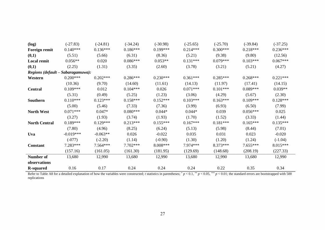
Education of adults is positively related to household per capita expenditure in urban

and rural areas, across the expenditure distribution, and in both survey periods. In

2002 at the median, an additional year of education increased household per capita

expenditure by 9 and 12 per cent in rural and urban areas respectively. By 2010 at the

median, the rural returns to education were 8.3 per cent and urban returns were 10.9

per cent. Further, the returns to education vary across the expenditure distribution;

returns to education of the urban sector remain higher than returns to education of the

rural sector. However, the returns between the two sectors became smaller across the

distribution – in the 25th quantile in 2002, the urban returns to education were 11.6 per

cent whereas rural returns to education were 6.6 per cent; by the 75th quantile, the

urban returns to education were 13.7 per cent and rural returns were 12.4 per cent.

Next, consider the employment type. Households with adults working in self-

employment consistently have higher per capita expenditure than comparable

households with adults working in wage employment or not employed/unemployed

across the expenditure distribution. Not being in the labour force has the greatest

negative association with per capita expenditure. This is true for both, urban and rural

areas. At any given point in the distribution, the returns to self-employment are higher

for urban households compared to rural households. In 2002, the returns to self-

employment in comparison to the returns to wage employment at the median were

45.2 per cent for urban households and 29.1 per cent for rural households. In 2010 at

the median, the urban returns were 37.8 per cent and rural returns were 19.1 per cent.

At a given point in time, the returns to self-employment rose across the expenditure

distribution – with the exceptions of urban households in 2009/10 and rural

households in 2002 when the returns remained fairly flat across the distribution. The

fact that self-employment pays higher returns than wage employment could come

across as an unusual finding. It can be explained in the following way. Parker (2009)

stressed that wage returns differ from returns to self-employment for several reasons –

firstly, it is difficult to interpret the salary of a self-employed individual as he/she

chooses to pay this for him/herself; secondly, the returns to self-employment are not

purely the return to labour, but also include the return to capital. Hence this finding

must be treated with caution.

Job sectors must be considered to further examine the changing returns to

employment. Households with adults working in agriculture have lower per capita

expenditure relative to households working in services or manufacturing industries.

This is in line with the finding observed by Thu Le and Booth (2014) in Vietnam.

Rural and urban households where adults are working in services had the highest per

capita expenditure – at the median, the returns to working in services was

approximately 17 per cent higher compared to working in agriculture in both years for

rural and urban households. For rural households, the returns from working in the

service industry increased across quantiles – from 12 per cent at the 25th quantile in

2002 to 23 per cent at the 75th quantile - suggesting that richer households got higher

returns from employment in this industry. A similar pattern was observed in 2009/10.

29

In urban areas, the coefficient on services does not vary across the distribution of

expenditure – this is true for both years.

The proportion of children and the natural log of household size measured the effects

of household demographics. The negative coefficient on household size suggests that

bigger households have lower per capita expenditure. Thu Le and Booth (2014)

found the same finding for Vietnam; the study also found that the proportion of

children inversely linked to per capita expenditure – however, the opposite finding

was observed for Sri Lanka where the presence of children in the household is linked

with higher per capita expenditure. The coefficients on these two demographic

variables become larger across the expenditure distribution suggesting that the

negative link between house size and per capita expenditure, and the positive link

between the presence of children and per capita expenditure are greater for richer

households. As observed in Section 4.2, the negative relationship between household

size and expenditure may possibly vanish at a size elasticity of 0.6 for rural

households due to size economies of consumption. However for urban households, we

observed a low value of the size elasticity (0.3) suggesting that larger households are

likely to have less expenditure.

The receipt of foreign and local remittances is positively associated with urban and

rural per capita expenditure in both years. Remittance flows were measured by a

dummy variable which had a value of 1 for households that received foreign/local

remittance income or a value of zero otherwise. Firstly, the impact of foreign

remittances on per capita expenditure is discussed. An urban (rural) household

obtaining foreign remittance had approximately 25 (19) per cent higher per capita

expenditure than their counterparts at the median of the expenditure distribution – the

coefficients are similar in both years. For rural households, the positive relationship

between foreign remittance and per capita expenditure rose greatly across the

expenditure distribution especially in 2010 – this implies that receiving foreign

remittance had a larger positive link with per capita expenditure for richer rural

households in comparison to poorer households. In 2009/10 at the 25th quantile, rural

households receiving foreign remittances had 14 per cent more per capita expenditure,

and at the 75th quantile, they were 30 per cent better off compared to those who did

not receive foreign remittances. Thu Le and Booth (2014) explained this in the

following way – in order for an individual in the family to migrate to a foreign

country for the purpose of working, the family will incur an initial cost (this cost

could be for travel, setting up, acquiring skills, learning the language). For poorer

households, this cost is likely to be covered by borrowing. Once the poor families

start receiving foreign remittances, they will first have to pay the borrowed money

back before they use the remittance receipt for their expenditure. Hence, a rich

household could have a larger increase in their expenditure once they have received

foreign remittances compared to poor households since they do not have to re-pay

borrowed money. For urban households receiving foreign remittances, in 2002 the

30

positive effect decreases across the expenditure distribution but in 2009/10 the effect

is fairly stagnant across the distribution.

Domestic remittances also had a positive association with urban and rural per capita

expenditure; however an exception was 2009/10 for urban households where local

remittances shared no significant association (at the 10 per cent level) with per capita

expenditure at any point in the distribution. In 2002 however, urban households

receiving domestic remittances had 22 per cent more per capita expenditure compared

to those who do not receive domestic remittances at the 25th quantile with the effect

becoming slightly larger for richer households (25 per cent). For rural households in

2002, receiving domestic remittances had an increasingly positive association with

per capita expenditure across the distribution suggesting that richer households further

benefitted from receiving this form of income. However in 2009/10, local remittances

had a significant and positive relationship with rural per capita expenditure at the

median and 75th quantile (at the 1 per cent significance level) but not at the 25th

quantile. The coefficient on the domestic remittance variable is however always

smaller than the coefficient of the foreign remittance variable; at the median in

2009/10, rural households receiving foreign remittances had 20 per cent higher per

capita expenditure relative to those who did not, whereas rural households receiving

local remittances saw a 5 per cent rise in per capita expenditure compared to those

who did not receive this income. This infers that households receiving income from

abroad are likely to have higher per capita expenditure compared to households

receiving domestic transfers.

Finally, the region dummy variables give some noteworthy findings. The Western

province has the highest living standards; this is true across urban and rural areas.

This is consistent with the fact that the capital city, Colombo, is a part of the Western

province. Colombo is the major economic centre in Sri Lanka and has the lowest

incidence of poverty. Although the Western province is primarily urban, almost 30

per cent of population in this province is from the rural sector according the Census of

Population and Housing (2011). Additionally, the findings show that the rural poor of

the Uva province have the lowest standard of living with the exception of the 75th

quantile.

The results obtained so far suggest that the return to working in certain types of

employment, education, and other household demographics are significant indicators

of urban and rural per capita expenditure. Further, regression estimations from the

pooled sample suggested that the urban dummy is highly significant – therefore, there

are urban-rural differences in per capita expenditure that can be explained by

differences between the two areas due to household endowments and the differences

in returns to endowments. Given the recent changes in the Sri Lankan economy

during the period of analysis, including the end of a civil war, growth of industry and

a reduction in poverty, our results are in line with these changes. Further, the

importance of remittances, services sector and education are in line with findings in

31

literature on other developing countries. The next section of the paper will identify the

contribution of each covariate used in the former regressions to the urban-rural

expenditure gap, and how the composition of the gap has changed over time.

6. Factors contributing to the urban-rural gap in expenditure

6.1 Method

The urban-rural differences in the distribution of log RPCE can be due to two

reasons – (1) differences in household characteristics between urban and rural

areas, or (2) differences in the returns to those characteristics between urban and

rural areas. As observed from the previous section, differences in returns do

explain the differences in per capita expenditure between households in urban and

rural areas – this section will look at the magnitude of the contribution and how it

has changed between 2002 and 2009/10 which will help explain the changing

pattern of the urban-rural welfare gap. More importantly, the impact of each

observable characteristic (for example, education) or the returns to those

characteristics (returns to education) on the urban-rural gap can be estimated. This

is done by applying a decomposition technique to the estimation results obtained

in the previous section - for urban and rural households.

In order to carry out this decomposition, the Blinder-Oaxaca decomposition

(Blinder, 1973; Oaxaca, 1973) is used14. The form of the decomposition is as

follows:

(5) �̂�𝑢 − �̂�𝑟 = (�̂�𝑢 − �̂�𝑟)�̂�𝑟 + (�̂�𝑢 − �̂�𝑟)�̂�𝑟 + (�̂�𝑢 − �̂�𝑟)(�̂�𝑢 − �̂�𝑟)

where Y is the natural logarithm of real per capita expenditure (RPCE) for the

household, hence �̂�𝑢 − �̂�𝑟 is the difference in log RPCE between urban and rural

areas. �̂� is a vector of observed characteristics, �̂� is a vector of estimated

coefficients obtained from running the regression model of log RPCE on a set of

explanatory variables and a constant. This is a three-fold decomposition, where

the differences in log RPCE can be explained in three parts.

The first part is given by:

(�̂�𝑢 − �̂�𝑟)�̂�𝑟

which is the expenditure differential that is due to differences in household

characteristics between urban and rural areas (the endowment effect).

14 The decomposition was run using the STATA command oaxaca8 by Firpo et al. (2009) which they employed in

their paper

32

The second part is given by:

(�̂�𝑢 − �̂�𝑟)�̂�𝑟

which is the expenditure differential that is due to differences in returns to

household characteristics between urban and rural areas (the coefficient effect). It

looks at the contribution of differences in coefficients of the urban and rural

household regressions (including differences in the intercepts) to the overall

expenditure gap.

The third part is given by:

(�̂�𝑢 − �̂�𝑟)(�̂�𝑢 − �̂�𝑟)

which is an interaction term accounting for the fact that there could be differences

in endowments and coefficients existing simultaneously between the two groups.

The decomposition given by Equation 5 is estimated from the viewpoint of rural

households; that is, the endowment effect measures the expected change for the

group of rural households’ mean expenditure per capita (or at a given quantile

which will be explained further below) if rural households had urban

characteristics. Similarly, the coefficient effect measures the expected change for

the group of rural households’ mean expenditure per capita (or at a given quantile)

if rural households received returns of urban households15.

A limitation of the Blinder-Oaxaca decomposition for the purpose of analysing

urban/rural expenditure differences across the entire distribution of expenditure is

that it could only be applied to the mean. The unconditional quantile regression,

however, as introduced by Firpo et al. (2009) obtains an estimate of the marginal

impact of a unit of change in any explanatory variable on the unconditional

quantiles of log RPCE (discussed in Section 5.1). This enables an application of

the Blinder-Oaxaca decomposition directly to the estimation results obtained from

the unconditional quantile regression.

There are two advantages of using this over other methods. Firstly, there is no

need to run several simulations – as is the case with the conditional quantile

regression decomposition put forward by Machado and Mata (2005). The

technique by Machado and Mata (2005) estimates the entire conditional

distribution Fx over a new distribution Gx in order to obtain a counterfactual

unconditional distribution of Y for rural households (where Y is the main variable

15 Alternatively, we can carry out a reverse three-fold decomposition to estimate the three effects from the

viewpoint of urban households. However, the command “oaxaca8” is used for decomposition at different

quantiles, rather than the “oaxaca” command for the decomposition at the mean – the former does not allow

estimation of the reverse decomposition.

33

of interest, log real per capita expenditure). The counterfactual distribution is then

compared with the empirical distributions for urban and rural households to

identify the differences in characteristics and returns to characteristics that exist

between the two groups. By contrast, RIF estimates the conditional distribution Fx

only at one specific point in the distribution. Secondly, the use of the Blinder-

Oaxaca decomposition allows us to isolate the contributions made by the

differences in urban-rural returns and characteristics from each explanatory

variable to the urban-rural expenditure gap at any given quantile along the

distribution.

6.2 Results

Table 5 reports the urban-rural expenditure gap in 2002 and 2009/10, along with

the contributing factors at the mean and selected quantiles. The total predicted gap

at a particular point in time rose across the expenditure distribution suggesting that

differences in per capita expenditure between urban and rural households are

higher amongst richer households – in 2002 (2009/10), the overall expenditure

gap between urban and rural households was 0.42 (0.25) log points at the 25th

quantile and rose to 0.60 (0.33) log points at the 75th quantile. Over time, the

expenditure gap has fallen sharply – at the median in 2002, the predicted gap was

0.51 log points and it fell to 0.30 log points by 2009/10. This fall in the urban-

rural welfare differences over time is in line with what we have observed in the

Sri Lankan economy, including the fall in poverty (particularly rural poverty),

high growth and the end of the war.

In both years, the urban-rural expenditure gap arose from two factors: the urban-

rural differences in endowments (differences in X terms of the regression), and the

differences in returns they get from those endowments16 (coefficients; that is,

differences in β terms). The welfare gap is reduced by the differences in

endowments interacted with the differences in returns (interaction terms; that is,

differences in X*β) – with one exception in 2002 (at the 25th quantile) where the

interaction effect led to an increase in the welfare gap. In 2002, the expenditure

gap can be explained more by the differences in returns rather than the differences

in endowments at any point on the distribution. In 2010, this is true at the 25th and

50th quantiles; however at the 75th quantile, the differences in endowments and the

differences in returns contribute equally to the overall expenditure gap. The

differences in characteristics interacted with the differences in the returns to

characteristics simultaneously (as given by the interaction term in the

decomposition) reduced the welfare gap, especially for the richest households – an

16 The rural returns are matched with urban characteristics to observe differences in returns between urban and

rural households; that is, how much rural households would receive if they were endowed with urban

characteristics

34

exception was noted in 2002 at the 25th quantile where the interaction effect

increased the welfare gap by 12 per cent.

In order to identify the underlying factors that contributed towards the differences

in endowments, returns and the simultaneous differences between the two former

effects, some key household characteristics will be examined and discussed.

Considerable differences in endowments between urban and rural households that

contribute towards the urban-rural expenditure gap will be discussed, namely

education, regional differences, sector of employment and employment activity.

Education was the largest contributing variable in both years – higher education

levels by urban households compared to rural households explained over 60 per

cent of the “endowment effect” at any point across the expenditure distributions in

2002; by 2010, the contribution of education differences increased across the

expenditure distribution from 58 to 63 per cent between the 25th and 75th

quantiles. At the median in 2002 (2009/10), differences in education levels

accounted for 0.14 (0.09) log points of the differences in per capita expenditure

between urban and rural households.

Regional differences were the second largest contributor towards the expenditure

gap as an endowment – approximately 30 per cent of the total endowment effect

was explained by regional differences. At the median, differences in regional

characteristics between urban and rural households contributed by 0.07 log points

to the expenditure gap in 2002, and by 0.05 log points in 2009/10. Across the

distribution, regional differences contributed more towards the higher welfare gap

at the top end of the expenditure distribution in 2002, whereas these differences

contributed less at higher quantiles in 2009/10.

Urban-rural differences in endowments by sector of employment (employment in

agriculture, manufacturing or services) had the third largest contribution towards

the endowment effect in both years. At the median, sectoral differences between

urban and rural households caused the expenditure gap to increase by 0.05 log

points in 2002 and 0.03 log points in 2009/10. In 2002, the differences by sector

of employment contributed by 20 per cent across the distribution, whereas in

2009/10, urban-rural differences in endowments by sector of employment

contributed by 13 per cent at the 25th quantile, increasing to a 21 per cent

contribution at the 75th quantile. This suggests that such differences have a smaller

role to play in explaining the expenditure gap for richer households compared to

poorer households.

Differences in the type of employment activity (wage, self-employed, not

employed) between urban and rural areas caused the expenditure gap to fall. In

2002 and 2009/10, at the median it explains 6 per cent of the total endowment

effect. In 2002 across the distribution, the differences contribute less towards the

35

endowment effect and overall gap at higher quantiles. However in 2009/10, these

differences contribute uniformly across the distribution. Other endowments where

urban-rural differences in the characteristics contributed towards a fall in the

welfare gap include urban-rural differences in age, household size and the

proportion of children. On the other hand, ethnic differences (significant at the 1

per cent level only in 2002) and the transfer of remittance income contribute to a

rise in the welfare gap.

Next, some key factors that contributed to the expenditure gap through the

differences in returns will be discussed. In both years, differences in the returns to

employment by age contributed towards a reduction of the “coefficient effect”;

although the contribution fell across the expenditure distribution especially in

2002 whereas other factors contributed to a rise in the welfare gap.

Urban-rural differences in returns to education had a large contribution towards

the coefficient effect. In 2002, the contribution of the differences in returns to

education at the median was 0.38 log points, and in 2009/10 the contribution was

0.17 log points. Across the distribution, the contribution of differences in returns

to education fell. In 2009/10, the contribution of this variable at the 25th quantile

was 0.16 log points; at the 75th quantile however, differences (0.12 log points)

contributed less to a higher endowment effect. This pattern observed by the

evolution of the urban-rural gap in returns to education for the lower and middle

parts of the expenditure distribution (0.38 log points at the median in 2002 and

reducing to 0.17 log points by 2009/10) contribute greatly towards the narrowing

of the overall urban-rural gap in per capita expenditure between 2002 and

2009/10.

In 2002, differences in returns to regional characteristics between urban and rural

households had a larger impact on richer households, whereas in 2009/10,

regional differences had no impact at the 75th quantile, but a large impact on

poorer households. This suggests that the differences in returns across regions

mattered primarily for the poor in 2009/10. While differences in returns to

education and regional characteristics matter less for the richer households in

2009/10, the intercept term is significant at the 1 per cent and contribute greatly

towards the welfare gap in 2009/10 at the 75th quantile. This term includes the

urban-rural differences in factors not captured in the model.

In 2009/10, the contribution of the constant term increased across the expenditure

distribution. However in 2002, this constant term was insignificant (at the 10 per

cent level) suggesting that the model included covariates that explain the

expenditure gap quite accurately. The paper by Thu Le and Booth (2014) noted

that the intercept was an important contributor at certain points in the distribution

for the Vietnam analysis; it was stated that factors such as infrastructure and

geographic conditions in favour of urban households might be useful in explaining

36

the gap. Unobservable factors, such as those discussed by Thu Le and Booth

(2014) can be possible explanations for the contribution of the intercept term

towards the overall coefficient effect in 2009/10 in our analysis.

Sectoral differences in returns contribute towards a reduction in the welfare gap,

especially in 2009/10. This suggests that the urban-rural differences in returns

from working in a particular industry (agriculture, manufacturing and services)

were more important in explaining the welfare gap of the rich. Other factors that

contributed towards the urban-rural gap include inter-group differences by returns

to ethnicity and remittances. The differences in returns by ethnic characteristics

explain a substantial part of the overall expenditure gap between urban and rural

areas in 2002, however the effects are smaller in 2009/10. Remittance flows

contribute by 7 per cent to the total coefficient effect at the 25th quantile, falling to

2 per cent at the 75th quantile in 2002. On the other hand in 2009/10, remittance

flows contribute towards a reduction of the coefficient effect by 10 per cent at the

highest quantile. Urban-rural differences in returns to demographic characteristics

(household size and the presence of children in the household) contribute towards

an increase in the welfare gap in 2002, and a decrease in the welfare gap in

2009/10.

The interaction effect measures the contribution of simultaneous differences in

characteristics and the returns to such characteristics across urban and rural

households towards the urban-rural welfare gap. In 2002, the interaction effect

increased the welfare gap by 12 per cent at the 25th quantile; however this

contribution fell across the distribution – at the 75th quantile, the interaction effect

contributed to a fall in the welfare gap by 14 per cent. In 2010, the interaction

effect reduced the welfare gap by 7 per cent at the 25th quantile; at the 75th

quantile, this effect contributed to a 12 per cent fall in the welfare gap.

To summarize, the decomposition results suggest that the welfare gap rises across

the distribution at a given point in time. Over time, the urban-rural welfare gap has

fallen. Overall, differences in characteristics such as education, job sector

(agriculture, manufacturing and services), regional differences and remittance

flows contribute to a higher welfare gap whereas differences in demographic

characteristics (household size and the presence of children) and job type (wage,

self-employed, unemployed/not employed) contribute to a lower gap. The

differences in returns to characteristics changed greatly over time – differences in

returns to education, job type and regions contributed less towards the gap at

higher quantiles. On the other hand, returns to unobservable characteristics have a

large role to play in 2009/10, especially for richer households.

For the purpose of comparison over time, we examined the determinants of per

capita expenditure for urban and rural households and estimated the urban-rural

welfare gap for the 17 districts included in both years. Tables A5, A6, and A7 in

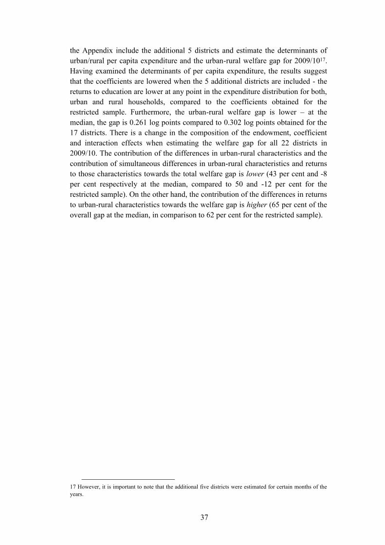
37

the Appendix include the additional 5 districts and estimate the determinants of

urban/rural per capita expenditure and the urban-rural welfare gap for 2009/1017.

Having examined the determinants of per capita expenditure, the results suggest

that the coefficients are lowered when the 5 additional districts are included - the

returns to education are lower at any point in the expenditure distribution for both,

urban and rural households, compared to the coefficients obtained for the

restricted sample. Furthermore, the urban-rural welfare gap is lower – at the

median, the gap is 0.261 log points compared to 0.302 log points obtained for the

17 districts. There is a change in the composition of the endowment, coefficient

and interaction effects when estimating the welfare gap for all 22 districts in

2009/10. The contribution of the differences in urban-rural characteristics and the

contribution of simultaneous differences in urban-rural characteristics and returns

to those characteristics towards the total welfare gap is lower (43 per cent and -8

per cent respectively at the median, compared to 50 and -12 per cent for the

restricted sample). On the other hand, the contribution of the differences in returns

to urban-rural characteristics towards the welfare gap is higher (65 per cent of the

overall gap at the median, in comparison to 62 per cent for the restricted sample).

17 However, it is important to note that the additional five districts were estimated for certain months of the

years.

38

Table 5: Contributions to the urban-rural expenditure gap at the mean and selected quantiles in 2002 and 2009/10

2002 2009/10

Q25th Q50th Q75th OLS Q25th Q50th Q75th OLS

Predicted

Gap

[�̂�𝒖 − �̂�𝒓]

0.423***

(26.55)

0.507***

(28.00)

0.598***

(30.71)

0.500***

(35.66)

0.252***

(18.53)

0.302***

(21.97)

0.333***

(20.69)

0.296***

(25.93)

Due to endowments [(�̂�𝒖 − �̂�𝒓)�̂�𝒓]:

Female 1.78x10-4

(0.42)

-1.88x10-4

(-0.41)

-0.001*

(-1.90)

-2.57x10-4

(-0.71)

-5.98x10-5

(-0.12)

-4.82x10-4

(-0.95)

-0.001**

(-2.06)

-0.001*

(-1.75)

Sinhalese 0.015***

(5.01)

0.010***

(3.63)

0.006**

(2.02)

0.012***

(5.12)

-2.71x10-4

(-0.14)

-3.31x10-4

(-0.19)

0.003

(1.56)

0.001

(0.92)

Age -9.64x10-4

(-1.31)

-0.004***

(-2.80)

-0.004**

(-2.51)

-0.003***

(-2.67)

-0.002***

(-2.68)

-0.005***

(-3.84)

-0.006***

(-3.46)

-0.005***

(-3.92)

Education 0.096***

(19.24)

0.136***

(21.63)

0.188***

(21.75)

0.148***

(22.99)

0.069***

(16.16)

0.090***

(17.68)

0.117***

(17.62)

0.097***

(18.50)

Job Type -0.012***

(-7.28)

-0.014***

(-7.37)

-0.013***

(-5.59)

-0.014***

(-9.09)

-0.009***

(-6.22)

-0.009***

(-5.75)

-0.011***

(-5.00)

-0.010***

(-7.49)

Job Sector 0.031***

(7.86)

0.050***

(12.03)

0.060***

(11.22)

0.041***

(12.61)

0.015***

(6.91)

0.034***

(10.20)

0.039***

(9.16)

0.027***

(9.98)

Demographics -0.023***

(-6.93)

-0.031***

(-7.29)

-0.035***

(-8.01)

-0.031***

(-7.97)

-0.015***

(-5.39)

-0.018***

(-5.39)

-0.020***

(-5.50)

-0.018***

(-5.50)

Remittances 0.004***

(3.46)

0.005***

(3.61)

0.005***

(3.05)

0.006***

(4.27)

0.004**

(2.62)

0.005***

(3.21)

0.008***

(3.53)

0.006***

(3.80)

Region 0.045***

(10.29)

0.067***

(13.32)

0.098***

(13.48)

0.067***

(16.35)

0.049***

(12.73)

0.053***

(13.30)

0.060***

(11.34)

0.052***

(15.67)

Total 0.155***

(18.41)

0.220***

(22.64)

0.301***

(24.02)

0.225***

(24.67)

0.119***

(16.14)

0.150***

(19.11)

0.187***

(19.13)

0.148***

(20.08)

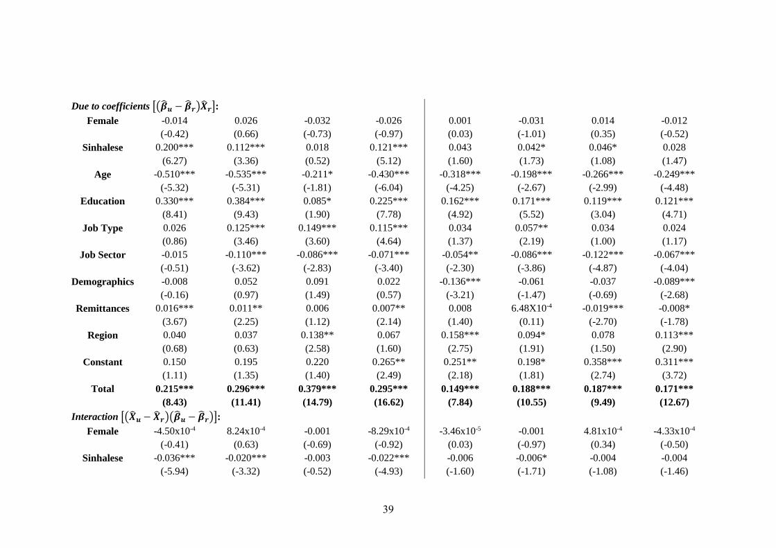
39

Due to coefficients [(�̂�𝒖 − �̂�𝒓)�̂�𝒓]:

Female -0.014

(-0.42)

0.026

(0.66)

-0.032

(-0.73)

-0.026

(-0.97)

0.001

(0.03)

-0.031

(-1.01)

0.014

(0.35)

-0.012

(-0.52)

Sinhalese 0.200***

(6.27)

0.112***

(3.36)

0.018

(0.52)

0.121***

(5.12)

0.043

(1.60)

0.042*

(1.73)

0.046*

(1.08)

0.028

(1.47)

Age -0.510***

(-5.32)

-0.535***

(-5.31)

-0.211*

(-1.81)

-0.430***

(-6.04)

-0.318***

(-4.25)

-0.198***

(-2.67)

-0.266***

(-2.99)

-0.249***

(-4.48)

Education 0.330***

(8.41)

0.384***

(9.43)

0.085*

(1.90)

0.225***

(7.78)

0.162***

(4.92)

0.171***

(5.52)

0.119***

(3.04)

0.121***

(4.71)

Job Type 0.026

(0.86)

0.125***

(3.46)

0.149***

(3.60)

0.115***

(4.64)

0.034

(1.37)

0.057**

(2.19)

0.034

(1.00)

0.024

(1.17)

Job Sector -0.015

(-0.51)

-0.110***

(-3.62)

-0.086***

(-2.83)

-0.071***

(-3.40)

-0.054**

(-2.30)

-0.086***

(-3.86)

-0.122***

(-4.87)

-0.067***

(-4.04)

Demographics -0.008

(-0.16)

0.052

(0.97)

0.091

(1.49)

0.022

(0.57)

-0.136***

(-3.21)

-0.061

(-1.47)

-0.037

(-0.69)

-0.089***

(-2.68)

Remittances 0.016***

(3.67)

0.011**

(2.25)

0.006

(1.12)

0.007**

(2.14)

0.008

(1.40)

6.48X10-4

(0.11)

-0.019***

(-2.70)

-0.008*

(-1.78)

Region 0.040

(0.68)

0.037

(0.63)

0.138**

(2.58)

0.067

(1.60)

0.158***

(2.75)

0.094*

(1.91)

0.078

(1.50)

0.113***

(2.90)

Constant 0.150

(1.11)

0.195

(1.35)

0.220

(1.40)

0.265**

(2.49)

0.251**

(2.18)

0.198*

(1.81)

0.358***

(2.74)

0.311***

(3.72)

Total 0.215***

(8.43)

0.296***

(11.41)

0.379***

(14.79)

0.295***

(16.62)

0.149***

(7.84)

0.188***

(10.55)

0.187***

(9.49)

0.171***

(12.67)

Interaction [(�̂�𝒖 − �̂�𝒓)(�̂�𝒖 − �̂�𝒓)]:

Female -4.50x10-4

(-0.41)

8.24x10-4

(0.63)

-0.001

(-0.69)

-8.29x10-4

(-0.92)

-3.46x10-5

(0.03)

-0.001

(-0.97)

4.81x10-4

(0.34)

-4.33x10-4

(-0.50)

Sinhalese -0.036***

(-5.94)

-0.020***

(-3.32)

-0.003

(-0.52)

-0.022***

(-4.93)

-0.006

(-1.60)

-0.006*

(-1.71)

-0.004

(-1.08)

-0.004

(-1.46)

40

Age -0.008**

(-2.62)

-0.006*

(-1.72)

-3.27x10-4

(-0.10)

-0.005

(-1.69)

-0.006***

(-2.98)

-0.003*

(-1.83)

-0.005**

(-2.37)

-0.005***

(-2.84)

Education 0.079***

(7.99)

0.092***

(8.84)

0.020*

(1.89)

0.054***

(7.44)

0.027***

(4.77)

0.029***

(5.32)

0.020***

(3.00)

0.020***

(4.58)

Job Type -0.006

(-1.49)

-0.008

(-1.35)

-0.013**

(-2.01)

-0.011***

(-2.78)

-0.008**

(-2.51)

-0.008**

(-2.20)

-0.006

(-1.29)

-0.006**

(-2.20)

Job Sector 0.004

(0.28)

-0.048***

(-3.44)

-0.048***

(-3.36)

-0.029***

(-2.97)

-0.015*

(-1.75)

-0.033***

(-3.84)

-0.047***

(-4.84)

-0.023***

(-3.68)

Demographics -0.003

(-1.00)

-0.010***

(-2.82)

-0.004

(-1.19)

-0.004*

(-1.85)

-0.004***

(-2.77)

-0.002

(-1.60)

-0.001

(-0.53)

-0.003**

(-2.21)

Remittances 0.004*

(1.79)

0.001

(0.48)

-0.001

(-0.49)

-4.73x10-4

(-0.30)

0.003

(0.88)

0.002

(0.78)

0.004

(1.19)

0.004*

(1.87)

Region 0.021*

(1.82)

-0.010

(-0.84)

-0.032**

(-2.32)

-0.003

(-0.37)

-0.007

(-0.71)

-0.014

(-1.57)

-0.002

(-0.19)

-0.008

(-1.11)

Total 0.053**

(2.57)

-0.009

(-0.42)

-0.083***

(-3.57)

-0.021

(-1.35)

-0.017

(-1.14)

-0.036**

(-2.57)

-0.041**

(-2.46)

-0.024**

(-2.21)

Number of

observations

16,920 16,920 16,920 16,920 17,182 17,182 17,182 17,182

The decomposition was estimated from the viewpoint of rural households. Base categories: Male (gender), non-Sinhalese (ethnic background), not employed (job type), agriculture (job

sector), Sabaragamuwa (region) z values in parentheses; Demographic characteristics include household size (log) and the number of children; * p < 0.10, ** p < 0.05, *** p < 0.01; the

standard errors are bootstrapped with 500 replications

41

7. Conclusion

In this paper, we examined the urban-rural welfare gap in Sri Lanka for the years

2002 and 2009/10. This was a period of transition, falling poverty and significant

growth for the economy. The data used for the analysis was from the Household

Income and Expenditure surveys carried out in 2002 and 2009/10. The study

contributes to existing literature in two significant ways. First, the urban-rural gap

has not been formally explored for Sri Lanka. Secondly, the paper adds to the

existing literature on urban-rural welfare gaps through the application of a new

method of unconditional quantile regression introduced by Firpo et al. (2009) used

to examine the determinants of per capita expenditure for urban and rural

households across the distribution of expenditure18. Using this method allowed the

contributions of individual factors to the overall urban-rural expenditure gap

across the distribution to be isolated. In order to do this, a variant of the Blinder-

Oaxaca decomposition was applied directly to the results obtained from the

unconditional quantile regression technique.

The focus on the entire expenditure distribution instead of looking at the mean

was beneficial since the pattern of the gap was not flat across the distribution. The

entire distribution was analysed through a quantile regression technique. Across

the distribution, the urban-rural welfare gap increased suggesting that there are

larger welfare differences across the two areas for richer households in both years.

After identifying the determinants of per capita expenditure for urban and rural

households, we observed that both, urban-rural differences in endowments (for

example, years of education) and the returns to those endowments (returns to

education) contributed towards urban-rural differences in per capita expenditure.

The study found that education levels of urban households, which were quite high

in the initial period to begin with, remained fairly similar across the analysed

period. In the rural sector however, education levels increased. The differences in

education levels contributed to a higher welfare gap for richer households in

2009/10. On the other hand regional differences, which also played an important

role in affecting the urban-rural welfare gap, contributed less to the welfare gap

for richer households in the latter period.

We also found that remittance flows, both local and foreign, have a positive

association with per capita expenditure in urban and rural areas; an exception was

seen in 2009/10 where local remittances had no significant link with urban per

capita expenditure. However, unlike in the case of Vietnam where the receipt of

local remittances narrowed the expenditure gap and foreign remittances widened

the gap (Thu Le and Booth, 2014); both, differences in foreign and local

18 To the best of my knowledge, this method has been applied to the urban-rural welfare gap in the case of

Vietnam. This is based on a literature search in EconLit.

42

remittance flows between urban and rural households contributed to a wider

welfare gap in the case of Sri Lanka. Other factors that contributed to the

expenditure gap include urban-rural differences in ethnicity, household size and

age, along with their respective returns.

Between 2002 and 2009/10, the urban-rural welfare gap reduced greatly at every

point in the expenditure distribution. Several factors contributed towards this.

Differences in certain endowments across urban and rural areas reduced during the

period. These included regional differences, differences in education levels, job

type (wage and self-employment) and job sector (agriculture, manufacturing and

services), and differences in demographic characteristics such as household size

and the number of children. Differences in returns to endowments also narrowed

in the latter period. Ethnic differences in returns were no longer significant

contributors towards the welfare gap. The differences in returns to education had

halved across the distribution by 2009/10; indicating that smaller differences in

returns to education contributed towards the overall urban-rural gap in welfare.

Another finding in the paper was that the differences in returns by type of

employment (wage and self-employment) were significant in affecting the large

urban-rural welfare gap in 2002, but had no significant impact on the gap in

2009/10 for richer households.

Such findings are in line with two important advances in Sri Lanka seen in recent

years – industrialization and the government’s focus on rural development. The

literature indicates that as the country became industrialized, more people started

moving away from agriculture to manufacturing and services. This was seen by

the rising contribution of services to GDP in recent years and the high returns to

working in services and manufacturing. Our results on the decomposition of the

wage gap suggested that, in addition to convergence of the composition of the

workforce across urban and rural households between 2002 and 2009/10, the

differences in sectoral returns (agriculture, manufacturing and services) across

urban and rural areas contributed to a large fall in the welfare gap in the latter

year.

By 2009/10, the war had ended and the country prioritized rural development.

Infrastructure developments meant that people were able to easily travel to towns

for employment. This rural-urban migration in the former years followed up by

the end of a 30-year war opening up new opportunities across the country are

consistent arguments with the findings of this study where the urban-rural

expenditure gap became smaller. During the analysed period, the country’s

industrialization has been favourable towards rural areas. However, the fact

remains that agriculture still gives the lowest returns in employment. Although the

significance of this industry has reduced in recent years, it still remains important

to a large proportion of rural households. Therefore, if the Sri Lankan government

focusses on poverty alleviation and reducing the urban-rural gap, our findings

43

suggest that support to poor rural households that will help them improve

agricultural productivity or move into other sectors such as services might be

helpful.

We identify certain limitations with the study. Firstly, education and potentially

other control variables such as occupation type are endogenous. As this analysis

was carried out at the household-level, the individual-level instruments used

previously are not appropriate. However as we include household characteristics

in this study, we hope that this helps reduce part of the bias caused by

disregarding unobservables (for example, by accounting for family background

effects directly in the model). As we observed the OLS estimates to be downward

biased at the individual level in the previous paper, we expect the effect of

education on the welfare gap to be under-estimated. The second limitation is the

lack of information on internal migration and road infrastructure in the HIE

surveys. The Institute for Policy Studies (2013) reported that the urban population

has remained fairly stable over the years at around 20 per cent. However to the

extent that migration took place, it might be a possible explanation for the

narrowing of the welfare gap over time. Infrastructure projects may have also

contributed to the welfare gap, making it easier for individuals/produce to be

moved across urban and rural areas. Further research to explore the improvements

in road infrastructure, migration and movements over time will be useful to

uncover these uncertainties. Finally, we note that the end of the war may have had

an effect on our results due to the displacement of people in war-affected areas of

the country. However, there is no available information on displacement.

Despite the above limitations, this paper adds to the literature through the

examination of the urban-rural welfare gap in Sri Lanka during a period of high

growth and falling poverty.

References

Blinder, A. S., 1973, “Wage Discrimination: Reduced Form and Structural Estimates”,

Journal of Human Resources, 8 (4), pp. 436–55

Central Bank of Sri Lanka, 2012, Annual Report (link:

http://www.cbsl.gov.lk/pics_n_docs/10_pub/_docs/efr/annual_report/AR2012/English/

7_Chapter_03.pdf)

Central Bank of Sri Lanka, 2009, Annual Report (link:

http://www.cbsl.gov.lk/pics_n_docs/10_pub/_docs/efr/annual_report/ar2009e/PDF/8_

chapter_04.pdf)

Deaton, A., 1997, The Analysis of Household Surveys: A Micro-econometric Approach to

Development Policy. Baltimore, MD: Johns Hopkins University Press

Department of Census and Statistics (various statistics including the HIES Final Report,

2009/10)

http://www.cbsl.gov.lk/pics_n_docs/10_pub/_docs/efr/annual_report/AR2012/English/7_Chapter_03.pdf

http://www.cbsl.gov.lk/pics_n_docs/10_pub/_docs/efr/annual_report/AR2012/English/7_Chapter_03.pdf

http://www.cbsl.gov.lk/pics_n_docs/10_pub/_docs/efr/annual_report/ar2009e/PDF/8_chapter_04.pdf

http://www.cbsl.gov.lk/pics_n_docs/10_pub/_docs/efr/annual_report/ar2009e/PDF/8_chapter_04.pdf

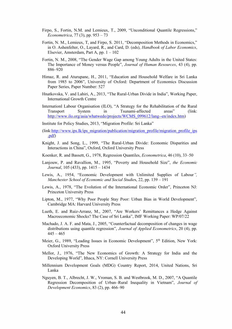
44

Firpo, S., Fortin, N.M. and Lemieux, T., 2009, “Unconditional Quantile Regressions,”

Econometrica, 77 (3), pp. 953 – 73

Fortin, N. M., Lemieux, T, and Firpo, S. 2011, “Decomposition Methods in Economics,”

in O. Ashenfelter, O., Layard, R., and Card, D. (eds), Handbook of Labor Economics,

Elsevier, Amsterdam, Part A, pp. 1 – 102

Fortin, N. M., 2008, “The Gender Wage Gap among Young Adults in the United States:

The Importance of Money versus People”, Journal of Human Resources, 43 (4), pp.

886–920

Himaz, R. and Aturupane, H., 2011, “Education and Household Welfare in Sri Lanka

from 1985 to 2006”, University of Oxford: Department of Economics Discussion

Paper Series, Paper Number: 527

Hnatkovska, V. and Lahiri, A., 2013, “The Rural-Urban Divide in India”, Working Paper,

International Growth Centre

Internationl Labour Organisation (ILO), “A Strategy for the Rehabilitation of the Rural

Transport System in Tsunami-affected areas” (link:

http://www.ilo.org/asia/whatwedo/projects/WCMS_099612/lang--en/index.htm)

Institute for Policy Studies, 2013, “Migration Profile: Sri Lanka”

(link:http://www.ips.lk/ips_migration/publication/migration_profile/migration_profile_ips

.pdf)

Knight, J. and Song, L., 1999, “The Rural-Urban Divide: Economic Disparities and

Interactions in China”, Oxford, Oxford University Press

Koenker, R. and Bassett, G., 1978, Regression Quantiles, Econometrica, 46 (10), 33–50

Lanjouw, P. and Ravallion, M., 1995, “Poverty and Household Size”, the Economic

Journal, 105 (433), pp. 1415 – 1434

Lewis, A., 1954, “Economic Development with Unlimited Supplies of Labour”,

Manchester School of Economic and Social Studies, 22, pp. 139 – 191

Lewis, A., 1978, “The Evolution of the International Economic Order”, Princeton NJ:

Princeton University Press

Lipton, M., 1977, “Why Poor People Stay Poor: Urban Bias in World Development”,

Cambridge MA: Harvard University Press

Lueth, E. and Ruiz-Arranz, M., 2007, “Are Workers’ Remittances a Hedge Against

Macroeconomic Shocks? The Case of Sri Lanka”, IMF Working Paper: WP/07/22

Machado, J. A. F. and Mata, J., 2005, “Counterfactual decomposition of changes in wage

distributions using quantile regression”, Journal of Applied Econometrics, 20 (4), pp.

445 – 465

Meier, G., 1989, “Leading Issues in Economic Development”, 5th Edition, New York:

Oxford University Press

Mellor, J., 1976, “The New Economics of Growth: A Strategy for India and the

Developing World”, Ithaca, NY: Cornell University Press

Millennium Development Goals (MDG) Country Report, 2014, United Nations, Sri

Lanka

Nguyen, B. T., Albrecht, J. W., Vroman, S. B. and Westbrook, M. D., 2007, “A Quantile

Regression Decomposition of Urban–Rural Inequality in Vietnam”, Journal of

Development Economics, 83 (2), pp. 466–90

http://www.ilo.org/asia/whatwedo/projects/WCMS_099612/lang--en/index.htm

http://www.ips.lk/ips_migration/publication/migration_profile/migration_profile_ips.pdf

http://www.ips.lk/ips_migration/publication/migration_profile/migration_profile_ips.pdf

45

Oaxaca, R., 1973, “Male-Female Wage Differentials in Urban Labor Markets,”

International Economic Review, 14 (3), pp. 693–709

Parker, S., 2009, “The Economics of Self-Employment and Entrepreneurship,”

Cambridge, Cambridge University Press

Sicular, T., Ximing, Y., Gustafsson, B. and Shi, L., 2007, “The Urban–Rural Income Gap

and Inequality in China”, Review of Income and Wealth, 53 (1), pp. 93–126

Thu Le, H. and Booth, A. L., 2014, “Inequality in Vietnamese Urban–Rural Living

Standards, 1993–2006”, Review of Income and Wealth, 60 (4), pp. 862–886

Uduporuwa, R. J. M, 2010, “An Analysis of Urban Growth and Urbanization in the

Sabaragamuwa Province, Sri Lanka”, Sabaragamuwa University Journal, 9 (1), pp.

115 - 132

UNDP, (link: http://www.lk.undp.org/content/srilanka/en/home/countryinfo.html) United

Nations Development Programme

World Bank, 2007, “Sri Lanka Poverty Assessment: Engendering Growth with Equity:

Opportunities and Challenges”, Poverty Reduction and Economic Management Sector

Unit: South Asia Region, Report No. 36568-LK

World Bank, 2009, “Sri Lanka Agricultural Commercialization: Improving Farmers’

Incomes in the Poorest Regions”, Poverty Reduction and Economic Management

Sector Unit: South Asia Region, Report No. 48968-LK

Appendix 1: Data on the excluded districts

Five districts were excluded from the analysis as they were not included in the

HIES held in 2002 due to the ongoing war. These include Jaffna, Vavuniya,

Batticaloa, Ampara and Trincomalee. In order to compare the characteristics of

these five districts to those included in the analysis, we explore the within-quintile

means for urban and rural households in the excluded districts. The descriptive

statistics are presented in Table A1. Some of the key differences are discussed as

follows. On average, households in the excluded districts have lower real

expenditure per capita at every quantile in comparison to the rest of the country.

This is especially true at higher quantiles where large differences in per capita

expenditure are observed. The household size in these five districts is smaller,

while the proportion of children are higher, compared to the other districts

included in the analysis. Adult non-students in these five districts are on average,

http://www.lk.undp.org/content/srilanka/en/home/countryinfo.html

46

younger, have lower levels of education, predominantly from a Tamil ethnic

background and have not received any form of remittance income. At lower

quantiles in urban areas, there are more employed adults in agricultural activities

and less in service-related activities compared to the rest of the country – such

differences are not present at higher quantiles. In rural areas, the proportion of

employed adults in agricultural activities is higher while the proportion of adults

in manufacturing and service-related activities is lower, compared to the rest of

the country.

47

Table A1: Within-Quintile Means of Key Variables by log RPCE for urban and rural households in 2009/10 (excluded districts)

The key variable of interest is “real per capita expenditure”, calculated in Sri Lankan rupees at 2002 prices (1 USD ≈ 146 LKR). The explanatory variables are computed using adult non-

student characteristics. Refer to Table A8 for a detailed explanation of how the variables were constructed. The category of not being in employment is the adult non-students who are

unemployed, retired/disabled and stay-at-home parents during the sample period. For the wage and self-employed adults, the sectoral variables capture the proportion of wage/self-

employed adults in agriculture, manufacturing or the services sector

2009/10 Urban (1,081 households) Rural (1,695 households)


RPCE (at 2002 prices) 1648 2359 2962 4018 8070 1345 1945 2406 3020 4873

Household size 5.29 4.73 4.59 3.85 3.49 5.26 4.69 4.27 3.98 3.34


Average age 30 31 32 36 40 29 31 33 35 35

Education 4.98 5.90 6.68 7.31 8.74 4.18 4.93 5.31 6.20 6.66

Women (prop.) 0.55 0.55 0.55 0.55 0.55 0.54 0.54 0.52 0.53 0.55

Sinhalese (prop.) 0.02 0.04 0.05 0.06 0.10 0.14 0.12 0.15 0.17 0.18

Local remit (0,1) 0 0 0 0 0 0 0 0 0 0

Foreign remit (0,1)

0 0 0 0 0 0 0 0 0 0

Wage (prop.) 0.20 0.21 0.22 0.23 0.31 0.22 0.22 0.23 0.23 0.25



Of the employed:



Services (prop.) 0.43 0.46 0.56 0.69 0.78 0.28 0.32 0.34 0.45 0.53

48

Appendix 2

Table A2: District-level Laspeyres price index

District Price Index Urban population (%)

2002 2009/10 2001 2011

Colombo 1.080 1.071 54.6 77.5

Gampaha 1.060 1.041 14.6 16.3

Kandy 1.020 1.007 12.2 12.1

Galle 1.030 0.993 11.1 12.0

Kalutara 1.070 1.038 10.6 9.2

Puttalama 1.000 1.008 9.2 9.3

Matara 0.980 0.961 8.5 11.8

Matale 0.980 0.985 8.2 14.1

Anuradhapura 0.970 0.980 7.1 5.4

Badulla 0.990 0.990 6.6 8.6

Nuwara-eliya 1.010 1.021 6.1 5.9

Ratnapura 1.020 0.991 5.7 8.9

Hambantota 0.940 0.979 4.1 5.5

Kurunegala 0.950 0.983 2.4 2.0

Kegalle 1.010 1.001 2.2 1.8

Polonnaruwa 0.960 1.001 0 0

Moneragala 0.960 0.974 0 0

Batticaloa 1.065 28.8

Mannar 26.0

Ampara 1.020 23.7

Trincomalee 1.052 22.8

Jaffna 1.075 21.0

Vauniya 1.032 20.7

Mullaitivu 0

Kilinochchi 0

Base for price index: Sri Lanka = 1; the population estimates were obtained from the Census of Population

and Housing carried out in 2001 and 2011. The districts were sorted by the proportion of individuals in urban

areas in 2001. The Household Income and Expenditure surveys do not disaggregate the districts further to

explore urban-rural compositions. The HIES for both years (2002 and 2009/10) were estimated using the

census blocks from 2001. The 2011 census has a similar composition, with Colombo being primarily urban

and Polonnaruwa and Moneragala being rural. Other districts are fairly similar on the urban-composition

scale over the years – exceptions include Matara, Matale, Badulla and Ratnapura which have become more

urbanized by 2011. The Northern and Eastern provinces (districts: Mannar, Ampara, Trincomalee, Jaffna,

Vavuniya, Mullaitivu and Kilinochchi) were excluded from the census in 2001 due to the war. Therefore, no

information on the price index and urban population is available for these areas. By 2009/10, 5 additional

districts were included in the survey and by 2011, all districts were included in the census.

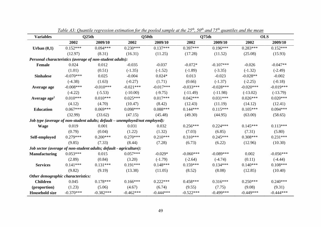
49

Table A3: Quantile regression estimation for the pooled sample at the 25th, 50th and 75th quantiles and the mean


2002 2009/10 2002 2009/10 2002 2009/10 2002 2009/10

Urban (0,1) 0.152***

(12.97)

0.094***

(8.31)

0.230***

(16.31)

0.137***

(11.25)

0.397***

(17.28)

0.196***

(11.52)

0.283***

(25.08)

0.152***

(15.93)


Female 0.024

(1.01)

0.012

(0.51)

-0.035

(-1.35)

-0.037

(-1.52)

-0.072*

(-1.89)

-0.107***

(-3.35)

-0.026

(-1.32)

-0.047**

(-2.49)

Sinhalese -0.070***

(-4.38)

0.025

(1.63)

-0.004

(-0.27)

0.024*

(1.71)

0.013

(0.66)

-0.023

(-1.37)

-0.028**

(-2.25)

-0.002

(-0.18)


(-4.22)

-0.010***

(-5.53)

-0.021***

(-10.00)

-0.017***

(-9.75)

-0.033***

(-11.49)

-0.028***

(-11.98)

-0.020***

(-13.02)

-0.019***

(-13.79)


(4.12)

0.010***

(4.70)

0.025***

(10.47)

0.017***

(8.42)

0.042***

(12.43)

0.031***

(11.19)

0.026***

(14.12)

0.020***

(12.41)

Education 0.067***

(32.99)

0.069***

(33.62)

0.098***

(47.15)

0.088***

(45.48)

0.144***

(49.30)

0.115***

(44.95)

0.105***

(63.00)

0.094***

(58.65)


Wage 0.019

(0.79)

0.001

(0.04)

0.031

(1.22)

0.032

(1.32)

0.256***

(7.03)

0.224***

(6.85)

0.145***

(7.31)

0.113***

(5.80)


(9.85)

0.200***

(7.33)

0.270***

(8.44)

0.210***

(7.28)

0.310***

(6.73)

0.245***

(6.22)

0.308***

(12.96)

0.231***

(10.30)


Manufacturing 0.053***

(2.89)

0.015

(0.84)

0.057***

(3.20)

-0.029*

(-1.79)

-0.060***

(-2.64)

-0.089***

(-4.74)

0.002

(0.11)

-0.056***

(-4.44)

Services 0.141***

(9.82)

0.131***

(9.19)

0.191***

(13.38)

0.148***

(11.05)

0.159***

(8.52)

0.134***

(8.08)

0.140***

(12.85)

0.108***

(10.40)


Children

(proportion)

0.045

(1.23)

0.178***

(5.06)

0.166***

(4.67)

0.222***

(6.74)

0.458***

(9.55)

0.316***

(7.75)

0.250***

(9.08)

0.240***

(9.31)

Household size -0.370*** -0.382*** -0.462*** -0.444*** -0.522*** -0.499*** -0.449*** -0.444***

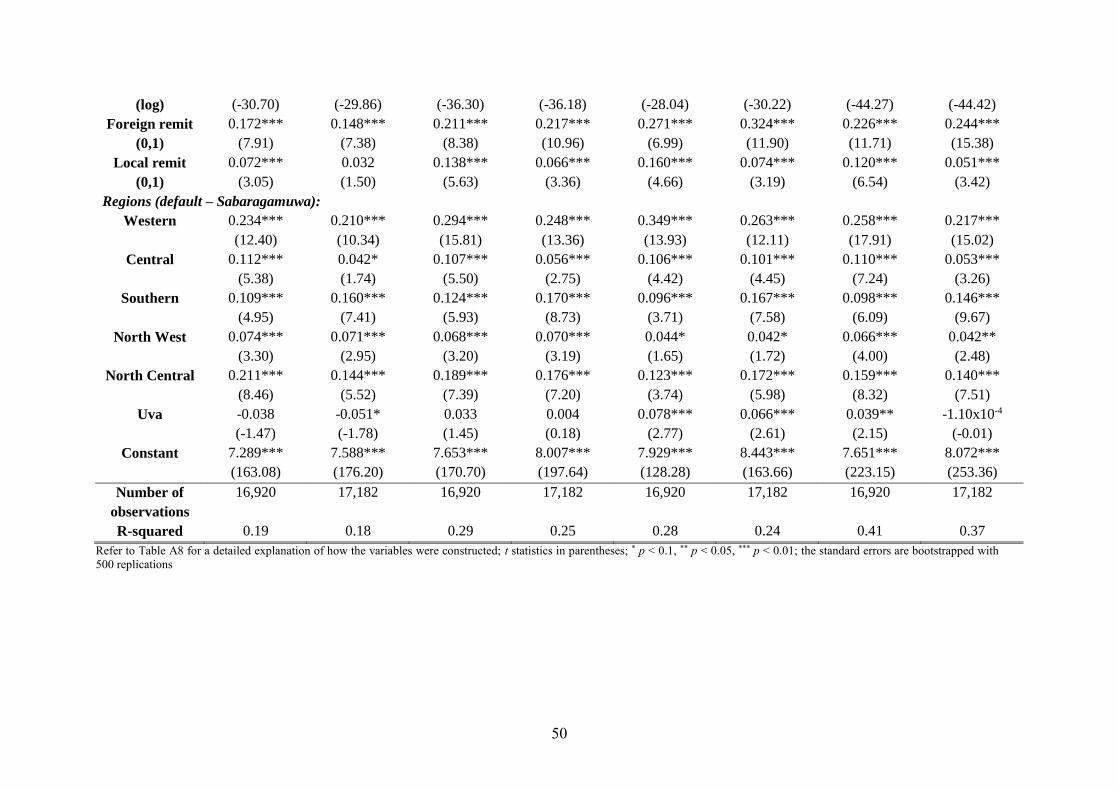
50

(log) (-30.70) (-29.86) (-36.30) (-36.18) (-28.04) (-30.22) (-44.27) (-44.42)

Foreign remit

(0,1)

0.172***

(7.91)

0.148***

(7.38)

0.211***

(8.38)

0.217***

(10.96)

0.271***

(6.99)

0.324***

(11.90)

0.226***

(11.71)

0.244***

(15.38)

Local remit

(0,1)

0.072***

(3.05)

0.032

(1.50)

0.138***

(5.63)

0.066***

(3.36)

0.160***

(4.66)

0.074***

(3.19)

0.120***

(6.54)

0.051***

(3.42)


Western 0.234***

(12.40)

0.210***

(10.34)

0.294***

(15.81)

0.248***

(13.36)

0.349***

(13.93)

0.263***

(12.11)

0.258***

(17.91)

0.217***

(15.02)

Central 0.112***

(5.38)

0.042*

(1.74)

0.107***

(5.50)

0.056***

(2.75)

0.106***

(4.42)

0.101***

(4.45)

0.110***

(7.24)

0.053***

(3.26)

Southern 0.109***

(4.95)

0.160***

(7.41)

0.124***

(5.93)

0.170***

(8.73)

0.096***

(3.71)

0.167***

(7.58)

0.098***

(6.09)

0.146***

(9.67)

North West 0.074***

(3.30)

0.071***

(2.95)

0.068***

(3.20)

0.070***

(3.19)

0.044*

(1.65)

0.042*

(1.72)

0.066***

(4.00)

0.042**

(2.48)


(8.46)

0.144***

(5.52)

0.189***

(7.39)

0.176***

(7.20)

0.123***

(3.74)

0.172***

(5.98)

0.159***

(8.32)

0.140***

(7.51)

Uva -0.038

(-1.47)

-0.051*

(-1.78)

0.033

(1.45)

0.004

(0.18)

0.078***

(2.77)

0.066***

(2.61)

0.039**

(2.15)

-1.10x10-4

(-0.01)

Constant 7.289***

(163.08)

7.588***

(176.20)

7.653***

(170.70)

8.007***

(197.64)

7.929***

(128.28)

8.443***

(163.66)

7.651***

(223.15)

8.072***

(253.36)

Number of

observations

16,920 17,182 16,920 17,182 16,920 17,182 16,920 17,182

R-squared 0.19 0.18 0.29 0.25 0.28 0.24 0.41 0.37

Refer to Table A8 for a detailed explanation of how the variables were constructed; t statistics in parentheses; * p < 0.1, ** p < 0.05, *** p < 0.01; the standard errors are bootstrapped with

500 replications

51

Table A4: Determinants of per household expenditure per capita at selected quantiles and mean (including interaction terms)


2002 2009/10 2002 2009/10 2002 2009/10 2002 2009/10

Urban (0,1) 0.086

(0.86)

0.111

(1.09)

0.179

(1.53)

0.079

(0.78)

0.317

(1.60)

0.133

(0.94)

0.265***

(2.79)

0.311***

(3.91)


Female 0.020

(0.69)

-0.016

(-0.55)

-0.041

(-1.37)

-0.052*

(-1.83)

-0.090**

(-2.20)

-0.089**

(-2.47)

-0.016

(-0.73)

-0.041*

(-1.86)

urban*female 0.021

(0.33)

0.074

(1.49)

0.014

(0.24)

0.054

(1.01)

0.114

(1.09)

-0.045

(-0.57)

-0.052

(-1.02)

-0.024

(-0.54)

Sinhalese -0.111***

(-5.26)

0.026

(1.25)

-0.050***

(-2.66)

0.009

(0.51)

-0.047**

(-2.27)

-0.042**

(-2.25)

-0.077***

(-5.24)

-0.012

(-0.90)

urban*sinhalese 0.131***

(4.39)

0.007

(-0.22)

0.159***

(4.78)

0.040

(1.36)

0.162***

(3.22)

0.076**

(2.01)

0.144***

(5.34)

0.036

(1.53)


(-2.95)

-0.009***

(-4.15)

0.018***

(-7.59)

-0.015***

(-7.52)

-0.023***

(-7.46)

-0.024***

(-9.43)

-0.013***

(7.63)

-0.015***

(-9.31)

urban*age -0.007*

(-1.69)

-0.004

(-1.05)

-0.013***

(-2.69)

-0.005

(-1.27)

-0.052***

(-6.38)

-0.011*

(-1.94)

-0.035***

(-8.77)

-0.015***

(-4.71)


(2.86)

0.009***

(3.65)

0.022***

(7.97)

0.015***

(6.34)

0.028***

(7.87)

0.027***

(8.61)

0.016***

(8.02)

0.015***

(8.18)

urban* age2 0.009*

(1.88)

0.002

(0.53)

0.016***

(2.79)

0.005

(1.15)

0.071***

(7.48)

0.013*

(1.87)

0.048***

(10.18)

0.016***

(4.35)

Education 0.074***

(31.27)

0.072***

(28.68)

0.099***

(42.39)

0.086***

(37.12)

0.128***

(39.15)

0.105***

(35.34)

0.097***

(52.12)

0.089***

(46.86)

urban*education -0.029***

(-6.43)

-0.013***

(-2.98)

-0.001

(-0.25)

0.005

(1.10)

0.069***

(8.11)

0.036***

(5.77)

0.036***

(8.20)

0.018***

(4.94)

52


Wage 0.014

(0.48)

0.035

(1.18)

0.028

(0.95)

0.025

(0.89)

0.186***

(4.74)

0.217***

(5.96)

0.087***

(3.97)

0.109***

(4.89)

urban*wage 0.045

(0.92)

-0.074

(-1.43)

0.005

(0.08)

0.075

(1.31)

0.346***

(3.13)

-0.019

(-0.22)

0.282***

(5.13)

0.012

(0.25)


(8.78)

0.218***

(6.71)

0.276***

(7.64)

0.206***

(6.17)

0.305***

(6.21)

0.232***

(5.30)

0.294***

(11.38)

0.223***

(8.82)

urban*Self-employed -0.090

(-1.48)

-0.029

(-0.51)

0.002

(0.02)

0.121*

(1.77)

0.293**

(2.03)

0.182*

(1.73)

0.222***

(3.20)

0.129**

(2.27)


Manufacturing 0.065***

(3.13)

0.018

(0.89)

0.083***

(4.18)

-0.010

(-0.58)

-0.035

(-1.45)

-0.060***

(-3.02)

0.033**

(2.19)

-0.029**

(-2.09)

urban*manufacturing -0.099**

(-2.30)

-0.074*

(-1.77)

-0.155***

(-3.00)

-0.137***

(-3.18)

-0.129

(-1.63)

-0.117**

(-2.04)

-0.157***

(-3.82)

-0.131***

(-4.00)

Services 0.145***

(9.05)

0.137***

(8.28)

0.203***

(12.89)

0.180***

(11.80)

0.204***

(10.44)

0.173***

(9.47)

0.162***

(13.78)

0.131***

(11.17)

urban*services -0.092***

(-2.58)

-0.081**

(-2.38)

-0.105**

(-2.43)

-0.177***

(-4.89)

-0.199***

(-2.89)

-0.138***

(-2.78)

-0.107***

(-3.08)

-0.107***

(-3.86)


Children (proportion) 0.075*

(1.77)

0.202***

(4.77)

0.179***

(4.52)

0.207***

(5.48)

0.400***

(7.95)

0.299***

(6.75)

0.221***

(7.31)

0.237***

(8.01)

urban*children -0.102

(-1.27)

-0.100

(-1.37)

-0.015

(-0.17)

0.065

(0.83)

0.359**

(2.51)

0.051

(0.48)

0.203***

(2.84)

-0.004

(-0.06)

Household size (log) -0.429***

(-30.16)

-0.403***

(-26.08)

-0.497***

(-34.17)

-0.450***

(-30.94)

-0.483***

(-23.51)

-0.462***

(-24.50)

-0.443***

(-39.17)

-0.422***

(-36.33)

urban*size 0.277***

(11.51)

0.084***

(3.08)

0.172***

(5.75)

0.042

(1.53)

-0.152***

(-3.08)

-0.116***

(-2.92)

-0.013

(-0.53)

-0.065***

(-2.86)

Foreign remit (0,1) 0.180***

(6.40)

0.163***

(6.24)

0.184***

(5.85)

0.213***

(8.55)

0.251***

(5.62)

0.307***

(9.40)

0.218***

(9.63)

0.236***

(12.25)

urban*foreign -0.054 -0.063 0.072 -0.009 0.048 0.032 0.020 0.005

53

(-1.40) (-1.60) (1.42) (-0.22) (0.54) (0.55) (0.46) (0.14)

Local remit (0,1) 0.064**

(2.36)

0.037

(1.56)

0.124***

(4.52)

0.070***

(3.26)

0.128***

(3.55)

0.076***

(3.14)

0.103***

(5.13)

0.067***

(4.17)

urban*local 0.047

(1.04)

-0.007

(-0.14)

0.073

(1.26)

0.021

(-0.39)

0.224**

(2.24)

-0.020

(-0.26)

0.120**

(2.44)

-0.095**

(-2.28)


Western 0.245***

(11.61)

0.228***

(10.16)

0.306***

(14.86)

0.254***

(12.32)

0.372***

(13.65)

0.249***

(10.47)

0.268***

(17.12)

0.221***

(13.80)

urban*western -0.151***

(-3.32)

-0.009

(-0.16)

-0.040

(-0.67)

0.043

(0.80)

0.122

(1.41)

0.191***

(2.77)

0.057

(1.26)

0.086**

(2.04)

Central 0.120***

(5.35)

0.017

(0.66)

0.094***

(4.56)

0.036*

(1.67)

0.071***

(2.92)

0.084***

(3.62)

0.089***

(5.57)

0.039**

(2.25)

urban*central -0.135***

(-2.65)

0.175***

(2.69)

0.066

(1.02)

0.138**

(2.20)

0.283***

(2.95)

0.147*

(1.83)

0.152***

(3.03)

0.118**

(2.42)

Southern 0.128***

(5.32)

0.143***

(5.95)

0.144***

(6.40)

0.155***

(7.25)

0.093***

(3.52)

0.146***

(6.30)

0.109***

(6.39)

0.128***

(7.80)

urban*southern -0.180***

(-3.37)

0.092

(1.55)

-0.106

(-1.61)

0.101*

(1.79)

0.145

(1.49)

0.190***

(2.65)

-0.005

(-0.10)

0.130***

(2.96)

North Western 0.077***

(3.24)

0.054**

(2.07)

0.061***

(2.73)

0.049**

(2.07)

0.025

(0.92)

0.020

(0.80)

-0.056***

(-3.27)

0.025

(1.41)

urban*north_w -0.092

(-1.58)

0.114*

(1.68)

0.078

(1.06)

0.162**

(2.48)

0.297***

(2.59)

0.251***

(2.99)

0.148**

(2.57)

0.167***

(3.22)


(8.49)

0.143***

(5.09)

0.199***

(7.35)

0.172***

(6.63)

0.121***

(3.57)

0.162***

(5.41)

0.165***

(8.30)

0.135***

(6.83)

urban*north_c -0.149***

(-2.62)

0.031

(0.41)

-0.034

(-0.40)

0.056

(0.74)

0.022

(0.17)

0.169

(1.62)

-0.062

(-0.91)

0.114*

(1.87)

Uva -0.028

(-1.02)

-0.072**

(-2.39)

0.031

(1.31)

-0.016

(-0.64)

0.034

(1.23)

0.040

(1.57)

-0.023

(-1.22)

-0.020

(-1.02)

urban_uva -0.090

(-1.19)

0.262***

(3.23)

0.025

(0.30)

0.211***

(2.66)

0.393***

(3.01)

0.242**

(2.28)

0.118*

(1.76)

0.215***

(3.40)

54

Constant 7.317***

(143.46)

7.574***

(150.12)

7.678***

(153.56)

8.018***

(173.65)

7.929***

(121.77)

8.418***

(148.70)

7.655***

(204.69)

8.015***

(221.74)

Number of

observations

16,920 17,182 16,920 17,182 16,920 17,182 16,920 17,182

R-squared 0.20 0.19 0.29 0.26 0.29 0.24 0.42 0.37


500 replications

Table A5: Determinants of urban household expenditure per capita at the mean and selected quantiles in 2009/10 (all districts)



Female 0.005

(0.12)

-0.068

(-1.44)

-0.072

(-1.23)

-0.067*

(-1.91)

Sinhalese 0.060**

(2.47)

0.063**

(2.48)

0.065**

(2.22)

0.056***

(2.93)


(-5.00)

-0.020***

(-5.65)

-0.030***

(-6.95)

-0.024***

(-9.34)


(4.31)

0.022***

(5.41)

0.034***

(6.61)

0.026***

(8.59)

Education 0.077***

(20.87)

0.098***

(25.98)

0.112***

(24.21)

0.097***

(32.62)


Wage -0.012

(-0.26)

0.111**

(2.11)

0.196***

(2.87)

0.086**

(2.13)


(4.88)

0.330***

(5.22)

0.372***

(4.57)

0.298***

(6.24)


Manufacturing -0.035

(-0.95)

-0.011

(-1.00)

-0.050

(-1.21)

-0.035

(-1.15)

55

Services 0.116***

(3.77)

0.141***

(3.58)

0.168***

(4.53)

0.143***

(4.03)


Children (proportion) 0.201***

(3.08)

0.217***

(3.69)

0.299***

(3.96)

0.200***

(4.10)


(-19.31)

-0.486***

(-20.55)

-0.475***

(-16.07)

-0.474***

(-25.73)


(6.86)

0.270***

(7.24)

0.246***

(5.22)

0.259***

(8.93)

Local remit (0,1) 0.069

(1.34)

0.016

(0.27)

-0.089

(-1.38)

-0.021

(-0.52)


Western 0.277***

(4.82)

0.295***

(5.60)

0.368***

(6.25)

0.304***

(7.39)

Central 0.204***

(3.10)

0.143**

(2.28)

0.193***

(2.80)

0.167***

(3.49)

Southern 0.278***

(4.70)

0.231***

(4.18)

0.302***

(4.87)

0.262***

(6.13)

Northern 0.250***

(3.52)

0.162**

(2.37)

0.230***

(3.02)

0.224***

(4.39)

Eastern 0.169**

(2.60)

0.045

(0.78)

0.151**

(2.36)

0.132***

(2.88)

North West 0.216***

(3.13)

0.197***

(3.05)

0.200***

(2.75)

0.203***

(3.96)

North Central 0.166**

(2.11)

0.208***

(2.69)

0.327***

(3.43)

0.247***

(4.08)

Uva 0.174**

(2.06)

0.184**

(2.22)

0.172*

(1.89)

0.199***

(3.14)

Constant 7.742***

(84.70)

8.132***

(88.75)

8.522***

(78.48)

8.240***

(119.85)

56


500 replications.

Table A6: Determinants of rural household expenditure per capita at the mean and selected quantiles in 2009/10 (all districts)



Female -0.024

(-0.97)

-0.024

(-0.99)

-0.075**

(-2.34)

-0.043**

(-2.22)

Sinhalese 0.013

(0.75)

-0.016

(-1.03)

-0.002

(-0.12)

0.004

(0.35)

Average age -0.004**

(-2.38)

-0.013***

(-7.21)

-0.022***

(-9.44)

-0.013***

(-9.16)

Average age2 0.003

(1.60)

0.012***

(5.84)

0.024***

(8.55)

0.013***

(7.77)

Education 0.060***

(28.58)

0.077***

(38.25)

0.101***

(38.15)

0.084***

(49.53)


Wage 0.014

(0.54)

0.017

(0.69)

0.146***

(4.38)

0.092***

(4.50)


(5.86)

0.175***

(6.10)

0.224***

(5.65)

0.201***

(8.77)


Manufacturing 0.010

(0.57)

-0.001

(-0.08)

-0.060***

(-3.23)

-0.033**

(-2.60)

Number of observations 5,273 5,273 5,273 5,273

R-squared 0.19 0.26 0.23 0.36

57

Services 0.108***

(7.81)

0.156***

(11.75)

0.174***

(10.37)

0.123***

(11.75)


Children (proportion) 0.148***

(4.15)

0.169***

(5.14)

0.272***

(6.70)

0.216***

(8.13)


(-27.81)

-0.422***

(-33.93)

-0.475***

(-28.50)

-0.420***

(-40.45)


(5.86)

0.197***

(8.56)

0.288***

(9.16)

0.234***

(12.69)

Local remit (0,1) 0.027

(1.24)

0.052***

(2.67)

0.065***

(2.80)

0.062***

(4.05)


Western 0.184***

(9.29)

0.224***

(11.64)

0.293***

(12.30)

0.225***

(14.72)

Central 0.008

(0.36)

0.027

(1.29)

0.087***

(3.63)

0.040**

(2.36)

Southern 0.112***

(5.24)

0.142***

(7.02)

0.154***

(6.50)

0.126***

(7.98)

Northern 0.064

(1.57)

-0.004

(-0.11)

-0.046

(-1.10)

0.006

(0.19)

Eastern 0.048*

(1.77)

0.012

(0.52)

-0.007

(-0.28)

0.008

(0.41)

North West 0.049**

(2.09)

0.045**

(2.05)

0.032

(1.21)

0.025

(1.45)


(4.92)

0.154***

(6.36)

0.176***

(5.81)

0.134***

(7.05)

Uva -0.058**

(-2.11)

-0.022

(-0.93)

0.018

(0.69)

-0.024

(-1.26)

Constant 7.610***

(176.15)

8.021***

(195.90)

8.396***

(160.60)

8.025***

(243.54)

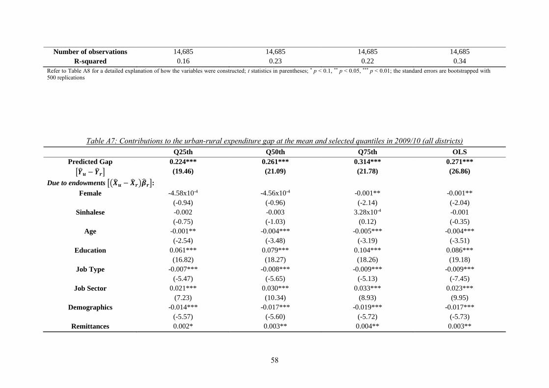
58


R-squared 0.16 0.23 0.22 0.34


500 replications

Table A7: Contributions to the urban-rural expenditure gap at the mean and selected quantiles in 2009/10 (all districts)

Q25th Q50th Q75th OLS

Predicted Gap

[�̂�𝒖 − �̂�𝒓]

0.224***

(19.46)

0.261***

(21.09)

0.314***

(21.78)

0.271***

(26.86)

Due to endowments [(�̂�𝒖 − �̂�𝒓)�̂�𝒓]:

Female -4.58x10-4

(-0.94)

-4.56x10-4

(-0.96)

-0.001**

(-2.14)

-0.001**

(-2.04)

Sinhalese -0.002

(-0.75)

-0.003

(-1.03)

3.28x10-4

(0.12)

-0.001

(-0.35)

Age -0.001**

(-2.54)

-0.004***

(-3.48)

-0.005***

(-3.19)

-0.004***

(-3.51)

Education 0.061***

(16.82)

0.079***

(18.27)

0.104***

(18.26)

0.086***

(19.18)

Job Type -0.007***

(-5.47)

-0.008***

(-5.65)

-0.009***

(-5.13)

-0.009***

(-7.45)

Job Sector 0.021***

(7.23)

0.030***

(10.34)

0.033***

(8.93)

0.023***

(9.95)

Demographics -0.014***

(-5.57)

-0.017***

(-5.60)

-0.019***

(-5.72)

-0.017***

(-5.73)

Remittances 0.002* 0.003** 0.004** 0.003**

59

(1.82) (1.99) (2.42) (2.41)

Region 0.033***

(9.40)

0.032***

(8.82)

0.036***

(7.78)

0.034***

(11.12)

Total 0.092***

(14.01)

0.113***

(15.90)

0.142***

(16.23)

0.116***

(17.32)

Due to coefficients [(�̂�𝒖 − �̂�𝒓)�̂�𝒓]:

Female 0.015

(0.59)

-0.023

(-0.83)

0.002

(0.05)

-0.012

(-0.59)

Sinhalese 0.034

(1.60)

0.033

(1.58)

0.048**

(1.99)

0.037**

(2.28)

Age -0.207***

(-3.28)

-0.087

(-1.32)

-0.108

(-1.38)

-0.169***

(-3.48)

Education 0.113***

(4.17)

0.130***

(4.75)

0.070**

(2.05)

0.082***

(3.75)

Job Type 0.008

(0.39)

0.048**

(2.09)

0.036

(1.20)

0.013

(0.76)

Job Sector -0.006

(-0.31)

-0.059***

(-3.27)

-0.081***

(-3.94)

-0.033**

(-2.43)

Demographics -0.093**

(-2.60)

-0.073*

(-1.90)

0.004

(0.08)

-0.076**

(-2.59)

Remittances 0.008

(1.64)

0.001

(0.20)

-0.014**

(-2.25)

-0.005

(-1.32)

Region 0.129**

(2.39)

0.089*

(1.81)

0.118**

(2.16)

0.119***

(3.08)

Constant 0.132

(1.30)

0.110

(1.10)

0.126

(1.04)

0.214***

(2.81)

Total 0.133***

(8.33)

0.170***

(10.86)

0.201***

(11.30)

0.170***

(14.41)

Interaction [(�̂�𝒖 − �̂�𝒓)(�̂�𝒖 − �̂�𝒓)]:

Female -5.59x10-4 -0.001 6.03x10-5 -4.56x10-4

60

(0.58) (-0.80) (0.05) (-0.58)

Sinhalese -0.008

(-1.60)

-0.007

(-1.58)

-0.011*

(-1.90)

-0.008**

(-2.27)

Age -0.004**

(-2.28)

-0.001

(-0.52)

-0.001

(-0.79)

-0.002**

(-2.03)

Education 0.018***

(4.08)

0.021***

(4.63)

0.011**

(2.04)

0.013***

(3.69)

Job Type -0.004*

(-1.68)

-0.006**

(-2.17)

-0.006

(-1.60)

-0.004*

(-1.84)

Job Sector 8.27x10-4

(0.12)

-0.020***

(-3.01)

-0.030***

(-3.87)

-0.011**

(-2.19)

Demographics -0.003**

(-2.54)

-0.003**

(-2.24)

-1.10x10-4

(-0.08)

-0.002**

(-2.09)

Remittances 4.29x10-4

(0.17)

0.003

(1.16)

0.005*

(1.72)

0.004**

(2.06)

Region -0.003

(-0.32)

-0.007

(-0.86)

0.002

(0.25)

-0.004

(-0.68)

Total -4.45x10-4

(-0.04)

-0.021*

(-1.73)

-0.029**

(-1.99)

-0.015

(-1.61)


The decomposition was estimated from the viewpoint of rural households. Base categories: Male (gender), non-Sinhalese (ethnic background), not employed (job type), agriculture (job

sector), Sabaragamuwa (region) z values in parentheses; Demographic characteristics include household size (log) and the number of children; * p < 0.10, ** p < 0.05, *** p < 0.01; the

standard errors are bootstrapped with 500 replications

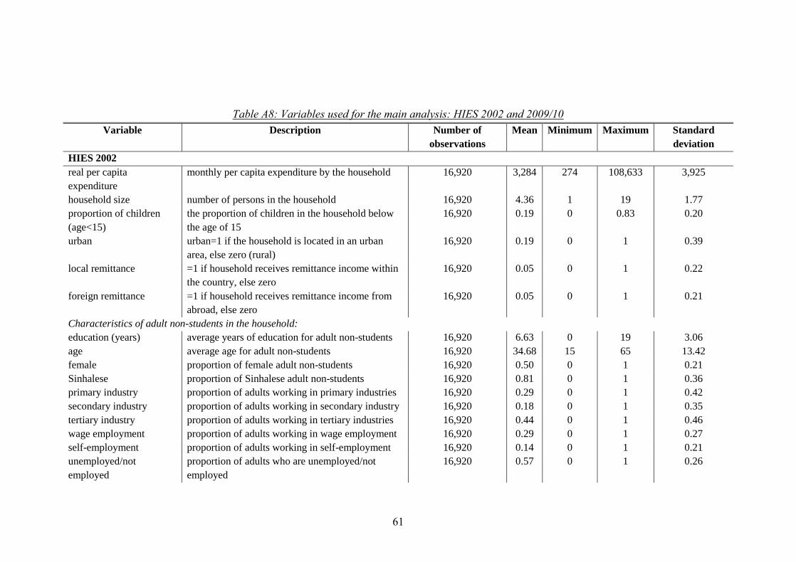
61

Table A8: Variables used for the main analysis: HIES 2002 and 2009/10

Variable Description Number of

observations

Mean Minimum Maximum Standard

deviation

HIES 2002

real per capita

expenditure

monthly per capita expenditure by the household 16,920 3,284 274 108,633 3,925

household size number of persons in the household 16,920 4.36 1 19 1.77

proportion of children

(age<15)

the proportion of children in the household below

the age of 15

16,920 0.19 0 0.83 0.20

urban urban=1 if the household is located in an urban

area, else zero (rural)

16,920 0.19 0 1 0.39

local remittance =1 if household receives remittance income within

the country, else zero

16,920 0.05 0 1 0.22

foreign remittance =1 if household receives remittance income from

abroad, else zero

16,920 0.05 0 1 0.21

Characteristics of adult non-students in the household:

education (years) average years of education for adult non-students 16,920 6.63 0 19 3.06

age average age for adult non-students 16,920 34.68 15 65 13.42

female proportion of female adult non-students 16,920 0.50 0 1 0.21

Sinhalese proportion of Sinhalese adult non-students 16,920 0.81 0 1 0.36

primary industry proportion of adults working in primary industries 16,920 0.29 0 1 0.42

secondary industry proportion of adults working in secondary industry 16,920 0.18 0 1 0.35

tertiary industry proportion of adults working in tertiary industries 16,920 0.44 0 1 0.46

wage employment proportion of adults working in wage employment 16,920 0.29 0 1 0.27

self-employment proportion of adults working in self-employment 16,920 0.14 0 1 0.21

unemployed/not

employed

proportion of adults who are unemployed/not

employed

16,920 0.57 0 1 0.26

62

HIES 2009/10

real per capita

expenditure

monthly per capita expenditure by the household

(at 2002 prices)

17,182

4,090

396

347,855

5,652

household size number of persons in the household 17,182 4.27 1 17 1.73

proportion of children

(age<13)

the proportion of children in the household below

the age of 15

17,182 0.17 0 0.75 0.19

urban urban=1 if the household is located in an urban

area, else zero (rural)

17,182 0.24 0 1 0.43

local remittance =1 if household receives remittance income within

the country, else zero

17,182 0.08 0 1 0.26

foreign remittance =1 if household receives remittance income from

abroad, else zero

17,182 0.07 0 1 0.25

Characteristics of adult non-students in the household:

education (years) average years of education for adult non-students 17,182 6.80 0 19 3.08

age average age for adult non-students 17,182 36.21 15 65 14.67

female proportion of women adult non-students 17,182 0.52 0 1 0.21

Sinhalese proportion of Sinhalese adult non-students 17,182 0.75 0 1 0.39

primary industry proportion of adults working in primary industries 17,182 0.26 0 1 0.41

secondary industry proportion of adults working in secondary

industries

17,182 0.20 0 1 0.36

tertiary industry proportion of adults working in tertiary industries 17,182 0.43 0 1 0.46

wage employment proportion of adults working in wage employment 17,182 0.26 0 1 0.27

self-employment proportion of adults working in self-employment 17,182 0.15 0 1 0.21

unemployed/not

employed

proportion of adults who are unemployed/not

employed

17,182 0.59 0 1 0.26

by Nirodha Bandara, Simon Appleton and Trudy Owens · Nirodha Bandara is the Directress of Academic...

Documents

Transcript of by Nirodha Bandara, Simon Appleton and Trudy Owens · Nirodha Bandara is the Directress of Academic...