
By JORGE J. AVILA S. - University of...
185
1 DETERMINING POTENTIAL DEMANDERS OF UREA BRIQUETTES IN THE CANTONS OF DAULE AND SANTA LUCIA IN THE ECUADORIAN COAST: EX-ANTE TECHNOLOGY ADOPTION ANALYSIS By JORGE J. AVILA S. A THESIS PRESENTED TO THE GRADUATE SCHOOL OF THE UNIVERSITY OF FLORIDA IN PARTIAL FULFILLMENT OF THE REQUIREMENTS FOR THE DEGREE OF MASTER OF SCIENCE UNIVERSITY OF FLORIDA 2012
Transcript of By JORGE J. AVILA S. - University of...

1
DETERMINING POTENTIAL DEMANDERS OF UREA BRIQUETTES IN THE CANTONS OF DAULE AND SANTA LUCIA IN THE ECUADORIAN COAST: EX-ANTE
TECHNOLOGY ADOPTION ANALYSIS
By
JORGE J. AVILA S.
A THESIS PRESENTED TO THE GRADUATE SCHOOL OF THE UNIVERSITY OF FLORIDA IN PARTIAL FULFILLMENT
OF THE REQUIREMENTS FOR THE DEGREE OF MASTER OF SCIENCE
UNIVERSITY OF FLORIDA
2012

2
© 2012 Jorge J. Avila S.

3
To Malena Santamaria, Alfredo A. “El Cholo”, Xavier A. and Belen M. son mi vida

4
ACKNOWLEDGMENTS
Firstly, I thank God for giving me everything. I will always thank my parents, my
family and Belen for their constant love. I am sincerely grateful to Dr. Bowen, Dr.
Espinel, Dr. Herrera, Dr. Sterns and Dr. Useche for the trust, support and contribution
that allowed me to develop this academic research. I would like to thank my great team
of enumerators Angie A., Karen R., Robinson M., Victor B., villagers of Daule and Santa
Lucia cantons and my friend Samuel whose invaluable help let me obtain the primary
data. I have to acknowledge Alfredo A., Belen M and Guido G. for having spent their
time on the tabulation of this thesis’ primary data. I would like to thank Centro de
Investigaciones Rurales of Escuela Superior Politecnica del Litoral, Food and Resource
Economics Department of University of Florida, the PL-480 of USDA and the Secretaria
Nacional de Educacion Superior, Ciencias, Tecnologias e Innovacion of Ecuadorian
government for having funded my master’s studies. I also thank Fatima at ESPOL and
Jessica at UF for having facilitated my life with all the paperwork. Last but not least, I
also thank all my friends, especially Amanda, Belinda, Clay, Imelda, Isnel, Lara, Lee,
Natasha and Olga who helped me in different ways during this time of my life.

5
TABLE OF CONTENTS page
ACKNOWLEDGMENTS .................................................................................................. 4
LIST OF TABLES ............................................................................................................ 7
LIST OF FIGURES .......................................................................................................... 8
LIST OF ABBREVIATIONS ........................................................................................... 11
ABSTRACT ................................................................................................................... 12
CHAPTER
1 INTRODUCTION .................................................................................................... 14
The Problem ........................................................................................................... 14 Research Question ................................................................................................. 16
Objective ................................................................................................................. 17 Thesis Structure ...................................................................................................... 17
2 LITERATURE REVIEW .......................................................................................... 20
Technology Adoption Overview .............................................................................. 20
Determinants of Adoption Decision ......................................................................... 25 Adoption Phases .............................................................................................. 25
Credit Market, Risk Aversion and Insurance .................................................... 26 Households’ Characteristics ............................................................................. 28
Farmers’ Characteristics................................................................................... 30 On-farm and Off-farm Activities and Non-work Income .................................... 32
Rice Production Factors ................................................................................... 33 Social Network and Information Sharing .......................................................... 35
3 UREA DEEP PLACEMENT TECHNOLOGY .......................................................... 37
Urea Deep Placement Functionality........................................................................ 37
Bangladeshi Experiences ....................................................................................... 39 Ecuadorian Experiences ......................................................................................... 42
4 ECUADORIAN RICE MARKET AT A GLANCE ...................................................... 49
5 METHODOLOGY.................................................................................................... 62
Sampling ................................................................................................................. 62 Unit of Analysis and Target Population............................................................. 62
Sampling Design .............................................................................................. 63

6
Questionnaire and Primary Data ............................................................................. 66 Theoretical and Empirical Model ............................................................................. 71
Theoretical Model ............................................................................................. 71 Empirical Model ................................................................................................ 74
6 EMPIRICAL RESULTS ........................................................................................... 80
Farmers’ Characteristics ......................................................................................... 80
Households’ Characteristics ................................................................................... 82 Urea Deep Placement Diffusion .............................................................................. 86
Social Network Analysis .......................................................................................... 88 Technology Adoption Analysis ................................................................................ 91
Rice Production System Analysis ........................................................................... 96 Credit and Insurance Market Analysis .................................................................. 102
Time Availability and Non-Work Income Analysis ................................................. 104 Econometric Results ............................................................................................. 105
Descriptive Summary of the Variables............................................................ 106 Tobit Estimation .............................................................................................. 109
Post-Estimation Analysis ................................................................................ 113
7 CONCLUSION REMARKS AND POLICY IMPLICATIONS .................................. 152
APPENDIX: QUESTIONNAIRE (SPANISH VERSION) ......................................... 159
LIST OF REFERENCES ............................................................................................. 178
BIOGRAPHICAL SKETCH .......................................................................................... 185

7
LIST OF TABLES
Table page 4-1 Rice production costs in 2011 (US$/ha) ............................................................. 57
4-2 World ranking of rice yield, 2000-10 (MT/ha) ...................................................... 59
4-3 Average international participation of the three types of rice, 2000-09 ............... 60
5-1 Target zones....................................................................................................... 78
6-1 Factors matrix (Factor Analysis) ....................................................................... 120
6-2 Coefficient matrix (Factor Analysis) .................................................................. 121
6-3 Statistics of those who knew and did not know about UDP .............................. 124
6-4 Time availability (hrs/day) ................................................................................. 146
6-5 Descriptive summary of dependent and independent variables ....................... 148
6-6 Tobit model estimation of Intensity of Adoption ................................................ 149
6-7 Collinearity evaluation of the independent variables......................................... 150

8
LIST OF FIGURES
Figure page 1-1 Fertilized rice land and total rice land in Ecuador .............................................. 19
3-1 Briquetting machine and Urea briquettes .......................................................... 46
3-2 Urea briquettes placement................................................................................. 46
3-3 Replication of briquetting machine and imported briquetting machine ............... 47
4-1 Rice production units and hectares by land size groups ..................................... 57
4-2 Rice yield (MT/ha), rice harvested land (ha) and rice production (MT), 2000-10 ....................................................................................................................... 58
4-3 Rice exports, rice imports and rice balance of trade-NX, fob (thousands, US$) ................................................................................................................... 60
4-4 Rice credit access (US$) .................................................................................... 61
5-1 Types of rice sowing ........................................................................................... 78
5-2 Distributions of applied surveys by sample ......................................................... 79
6-1 Farmers’ gender ............................................................................................... 116
6-2 Farmers’ age .................................................................................................... 116
6-3 Education.......................................................................................................... 117
6-4 Agricultural education ....................................................................................... 117
6-5 Types of agricultural ......................................................................................... 118
6-6 Agricultural education providers ....................................................................... 118
6-7 Land size groups .............................................................................................. 119
6-8 Rented land ...................................................................................................... 119
6-9 Total expenses by land size groups ................................................................. 120
6-10 Wealth index ..................................................................................................... 121
6-11 Wealth level ...................................................................................................... 122
6-12 Drought and flood affectation............................................................................ 122

9
6-13 Time to get the main town by spent time groups (Market Access) ................... 123
6-14 UDP knowledge ................................................................................................ 123
6-15 UDP knowledge sources .................................................................................. 124
6-16 Observable UDP results ................................................................................... 125
6-17 UDP knowledge level ....................................................................................... 125
6-18 Agricultural group affiliation .............................................................................. 126
6-19 Agricultural groups’ names ............................................................................... 126
6-20 Meeting frequency ............................................................................................ 127
6-21 Voluntary attendance ........................................................................................ 127
6-22 Farmers’ behavior in meetings ......................................................................... 128
6-23 Influential groups .............................................................................................. 128
6-24 Communication level ........................................................................................ 129
6-25 Past technology adoption ................................................................................. 129
6-26 Adopted innovations ......................................................................................... 130
6-27 WTP: first question with initial bid by land size groups ..................................... 130
6-28 WTP: second question with higher bid ............................................................. 131
6-29 WTP: second question with lower bid ............................................................... 131
6-30 WTP (US$) by land size groups ....................................................................... 132
6-31 EWTP: first question with initial bid by land size groups ................................... 132
6-32 EWT: second question with higher bid ............................................................. 133
6-33 EWTP: second question with lower bid ............................................................ 133
6-34 EWTP (US$) by land size groups ..................................................................... 134
6-35 UDP potential area (ha) .................................................................................... 134
6-36 Intensity of Adoption by land size groups (%) ................................................... 135
6-37 Rice field ........................................................................................................... 135

10
6-38 Description of rice varieties (in Spanish) .......................................................... 136
6-39 Rice variety ....................................................................................................... 136
6-40 Soil preparation cost (US$/ha) by tillage tractor ............................................... 137
6-41 Total seed costs (US$/ha) plotted with land size (ha) ....................................... 137
6-42 Urea (50-kg sacks/ha) by land size groups....................................................... 138
6-43 Urea prices (US$/sack) of subsidized, real and black markets ......................... 138
6-44 Total cost of other fertilizers (US$/ha) by land size groups .............................. 139
6-45 Total cost of herbicides/pesticides (US$/ha) by land size groups ..................... 139
6-46 Total cost of hired labor .................................................................................... 140
6-47 Total irrigation cost (US$/ha) by land size groups ............................................ 140
6-48 Total harvest cost (US$) by land size groups ................................................... 141
6-49 Rice yield (kg/ha) by land size groups .............................................................. 141
6-50 Rice sack sold (%) by land size groups ............................................................ 142
6-51 Total income (US$/ha) by land size groups ...................................................... 142
6-52 Credit Solicitation .............................................................................................. 143
6-53 Credit providers ................................................................................................ 143
6-54 Credit (US$) by land size groups ...................................................................... 144
6-55 Uses of the credit .............................................................................................. 144
6-56 Rice insurance .................................................................................................. 145
6-57 Main occupation ............................................................................................... 145
6-58 Non-work income .............................................................................................. 146
6-59 Human Development Bonus (US$) .................................................................. 147
6-60 Intensity of Adoption Residuals ........................................................................ 151
6-61 Jarque-Bera Normality test of Residuals .......................................................... 151

11
LIST OF ABBREVIATIONS
BM Briquetting Machine
HA Hectare
HYVs High-Yielding Varieties
HR Hour
IA Intensity of Adoption
Kg Kilogram
MT Metric Ton
N Nitrogen
PUS Production Units
USDA United States Department of Agriculture
UBS Urea Briquettes
UDP Urea Deep Placement
WTP Willingness to Pay with Economic Benefits/Cost
EWTP Willingness to Pay with Economic Benefits/ Costs and Environmental Impacts

12
Abstract of Thesis Presented to the Graduate School of the University of Florida in Partial Fulfillment of the
Requirements for the Degree of Master of Science
DETERMINING POTENTIAL DEMANDERS OF UREA BRIQUETTES IN THE CANTONS OF DAULE AND SANTA LUCIA IN THE ECUADORIAN COAST: EX-ANTE
TECHNOLOGY ADOPTION ANALYSIS
By
Jorge J. Avila S.
December 2012
Chair: Pilar Useche Cochair: James Sterns Major: Food and Resource Economics
In Ecuador, the main fertilizer for rice cultivation, Urea, may be lost as much as
60% when it is applied with Broadcast technique. Urea Deep Placement (UDP),
originally utilized in Asia, has been shown to enable rice farmers to reduce such a loss.
This thesis is an ex-ante analysis of the potential for UDP adoption in two major rice
producing cantons in the Ecuadorian Coast, Daule and Santa Lucia. A survey was
implemented to collect information of rice farmers across 35 villages. A descriptive
analysis explored variables that may affect adoption decision. For instance, some
farmers obtained negative net incomes, implying the need of more efficient innovations
like UDP. In the Double-bounded exploratory analysis was detected that 93.25% of the
sample farmers were willing to pay extra for Urea briquette sacks with the introduction
economic benefits/costs and with the inclusion of economic and environmental impacts.
In analyzing the Intensity of Adoption (IA), potential adopters would dedicate a 49.7% of
their total land for UDP production, on average. Finally, the two-limit Tobit model of the
technology adoption decision (in terms of the IA) suggests that the smaller a farmer, the
higher his probability of UDP adoption. However, the subsidy of Urea fertilizer may be

13
an obstacle for UDP acceptance. Social network was also significant in the model;
potential adopters’ behaviors may influence a farmer’s adoption decision. Other
significant variables were small kids in a household, market access, rented land, credit
solicitation, agricultural insurance, risk aversion, UDP knowledge and on-farm hours.

14
CHAPTER 1 INTRODUCTION
According to the Food and Agriculture Organization (2011), rice consumption has
increased rapidly in developing countries where rice intake was expected to raise by
461 million tons (3% more than 2010); per capita world rice consumption was 57
kg/year, on average, in 2011 (half a kilogram higher than in 2010). Moreover, around
half of the world population has this cereal as a staple food (International Rice Research
Institute 2012). In Ecuador, rice is important in term of diet, whose per capita
consumption is 112 kg/year. But also, it is the main occupation for 75,813 production
units. Additionally, small farmers are ensuring the access to this grain as 80% of rice
production units are small, less than 20 ha (Instituto Nacional de Estadística y Censos,
Ministerio de Agricultura, Ganaderia, Pesca y Acuacultura and Sistema de Informacion
Agraria 2012). However, small farmers are struggling against poverty; official statistics
shows that 50.9% of the rural population was poor in 2011(Instituto Nacional de
Estadística y Censos 2012). Also, the most important rice producing zones, Guayas and
Los Rios, are part of the provinces with the greatest number of poor people in rural
zones, around 350000 and 250000 habitants respectively (see Manuel Chiriboga y
Brian Wallis 2010).
At national level, rice is also relevant for Ecuador. In 2009, rice production
contributed to the Agricultural Growth National Product and the Growth National Product
in 11.49% and 0.69% respectively (Instituto Nacional de Estadística y Censos 2011).
The Problem
The most important fertilizer for rice crops is Urea. According to the Instituto
Nacional de Preinversion (2011), the total Urea demand is determined in about 500,000

15
MT in Ecuador; mean Urea importation was 270,000 MT, during 2009-11. Particularly,
the 2011 Urea importation was 291,114 MT (in monetary terms, US$146,645,000);
comparing the first quarter of 2011 and 2012, urea importation decreased in 14.9%
(Sistema de Información Nacional de Agricultura, Ganadería, Acuacultura y Pesca
2012). In 2011, farmers could access Urea sacks (50 kg) at a subsidized price of
US$10; having a market price of around US$25. Thus, the government paid the 60% of
the price (Banco Central del Ecuador 2011). This is the pressure that Ecuador must
face as a non-producer of Urea given the absence of infrastructure to produce this
fertilizer1.
Knowing the actual situation of Ecuador with respect to Urea fertilizer, it is time to
define the problem inside the rice sector. As is well known, Urea is the main fertilizer
applied on rice crops. Ecuadorian rice farmers principally apply Urea by throwing it on
their crops; such technique is called “broadcast fertilization” (Alvoleo, in Ecuador). N. K.
Savant and P. J. Stangel (1990) determined that this fertilization technique entails to a
loss of Urea up to 60%, which is provoked by NH3 volatilization, denitrification, leaching,
and/or runoff. To observe the magnitude of this problem, let’s first take a look at the
fertilized and total rice land over time in Ecuador (see Figure 1-1). One can observe that
the majority of rice land has been fertilized over time; 97%, on average. The greatest
amount of fertilized land was 416,416 ha in 2004, followed by 413,266 ha in 2009.
However, between 2005 and 2006, fertilized land dedicated to rice production dropped
42%; maybe, this reduction was caused by the adverse climatic situation, low prices,
etc. Since 2008, both types of lands were recovered.
1 Instituto Nacional de Preinversion 2011 pointed out that Ecuador has been developing a plan to start the
production of urea.

16
Considering the 2010 fertilized land and assuming that everyone used 200 kg/ha
of Urea needed to fertilize the rice crop, according to Achim Dobermann (2012). In total,
80,751.6 MT of Urea could have been used for 403,758 ha. As mentioned above, given
the Urea loss of 60%, 29,070.58 MT could have lost because of the inefficient
Broadcast application. This value could have represented, on average, a 10.78% of the
imported Urea over time (last two years).
A potential solution to this problem is the adoption of Urea Deep Placement, which
promises more benefits than costs at different levels. For instance, the farm-level
benefits and costs are: Urea saving up to 40%; yield increase up to 25% (per se income
increase); reduction of weed-control cost; labor increase (hired and/or family) and;
harvest cost augmentation. At national level, the benefits from adopting this technology
are: employment creation (production of Urea briquettes, briquetting machines and day
laborer requirement by farmers); gender income equity; Urea import decline; reduction
of Urea subsidy pressure and; reduction of N in the atmosphere and water resources
(International Fertilizer Development Center 2008). These impacts motivate the
development of UDP adoption analysis in this thesis.
Research Question
In Ecuador, UDP was also introduced to reduce Urea loss. Some rice farmers and
students from Escuela Superior Politecnica del Litoral several UDP trials, during 2009-
10. There were reduction on Urea fertilizer cost of up to 44.75%; corroborating the
efficiency of this method. Additionally, rice yield ranged was improved, obtaining
increases in a range of 8.92% to 56.22% (Escuela Superior Politecnica del Litoral,
University of Florida and PL-480 of USDA 2008). These results were diffused through
several communication channels: radio, press, television, extension work and

17
agricultural fairs. As a result, there is an interest of responding the following research
question:
What would be the incentives and constraints that may make an Ecuadorian rice famer be willing to adopt the Urea Deep Placement Technology?
Objective
UDP was brought to Ecuador by Escuela Superior Politecnica del Litoral,
University of Florida and PL-480 of USDA (2008). As UDP is a new technology going
into the rice farmers, there is still a need of research about this innovation. Moreover, a
big restraint of this innovation is the production of the Briquetting Machine whose cost is
about US$7500 in Ecuador (Orlando D. Contreras and Marcelo Espinosa L. 2010);
while, the importation cost was estimated in US$2000. Thus, the objective of this thesis
is to:
Present valuable information about the potential demanders of UDP technology to possible briquette investors in order to create a Briquette Market in Ecuadorian Coast; and finally, provide general information to policymakers for implementation of agricultural policies.
In determining such demand, I could encourage investors to participate in the
production of this machine. In order to answer the research question and reach the
objective, a questionnaire was designed to estimate a Tobit model through which I
establish what factors may affect UDP adoption and perhaps, agricultural innovation in
general.
Thesis Structure
Without including the Introduction, this thesis is finally organized as follows:
Chapter 2 reviews the agricultural adoption literature in which the main factors affecting
adoption decision are described. Chapter 3 presents the results of UDP adoption in

18
Bangladesh and those experiments’ outcomes in Ecuador. Chapter 4 describes
important variables of the Ecuadorian rice market. Chapter 5 introduces the sample
design, the survey instrument and, the theoretical and empirical model used in this
study. Chapter 6 reports a descriptive analysis and the Tobit estimation outcomes with
the collected data in Daule and Santa Lucia cantons. Finally, Chapter 7 presents the
conclusions and policy implications of this thesis.

19
Figure 1-1. Fertilized rice land and total rice land in Ecuador (Source: Ecuador en cifras
2012. http://www.ecuadorencifras.com/cifras-inec/main.html. (accessed June 10, 2012).)

20
CHAPTER 2 LITERATURE REVIEW
In countries like Ecuador, small farmers are ensuring food access to an entire
nation. Contradictory, those farmers are the poorest and commonly suffer famine, with
children and young people being the most stricken (Organización de las Naciones
Unidas para la Agricultura y la Alimentación, Fondo Internacional de Desarrollo Agrícola
and Programa Mundial de Alimentos 2002). Such a problem can be overcome with the
productivity improvements in farming, ensuring income and food access. One response
to accomplish this objective is the introduction of improved technologies which would
allow enhancing farmers’ welfare; thus, farmers keep producing staple food, such as
rice (Timothy Besley and Anne Case 1993; Cheryl R. Doss 2006). As a result, UDP
adoption could represent an important improvement for Ecuadorian agriculture. Indeed,
UDP would accomplish those required objectives to ensure food security: food must
come from environmental and efficient innovations that take into consideration the
biodiversity (see Magdalena Kropiwnicka 2005). Given the aforementioned reasons, the
potential determinants and conceptual foundations of the technology adoption are
explored in this section.
Technology Adoption Overview
In defining an agricultural innovation or technology, diverse conceptions are found.
Mahajan and Perteson (1985) defined any new idea, practice or object implemented in
the agriculture as a technology (see Lawrence Loh and N. Venkatraman 1992).
Gershon Feder and Dina L. Umali (1993) provided a more complete definition: a
technology is referred to a factor which modifies the way how a farmer produces, where
uncertainties can be undermined with experiences over time.

21
All these three definitions are consistent with what UDP represents: a new
method/idea/factor going to change rice farmers’ production function. Now, a discussion
is presented about technologies that were introduced in agriculture in two important
periods of times: Green Revolution and Biotechnology Era. These two periods were
taken into account because they are breaking points for agriculture development.
Technological changes or innovations have been proven to have a great influence
in the economic progress in The Green Revolution. The introduction of such
technologies improved the capability of a farmer to produce a certain crop. High
Yielding Varieties (HYVs), inorganic fertilizers, other chemical inputs and water control
were the most accepted innovations in developed and developing countries, during the
1940s and 1970s. For instance, the widely recognized and named “Father of the Green
Revolution”, Norman Borlaug, introduced the high-yield wheat to combat starvation
worsened by the rapid population growth, first in Mexico and later in Asia. According to
the International Food Policy Research Institute (2002), the problem of starvation in
industrial countries could be avoided by the adoption of improved plant breeding,
fertilizers and pesticides during the half of the 20th century. R. E. Evenson and D. Gollin
(2003) carried out a study of the adoption of HYVs over developing countries. They first
defined two periods of time, Early and Late Green Revolution, being the difference that
in the late one the adoption of improved varieties had a greater positive impact of yield
growth across all developing regions (Asia, Latin American, Middle-East North Africa
and Sun-Saharan Africa). In the early era, Asia and Latin American nations were the
regions that most benefited from HYVs. While in the late era, they found that the rest of
the regions reached an improvement of yield when suitable HYVs were introduced.

22
Haitao Wu et al. (2010) demonstrated that the adoption of HYVs and chemical fertilizers
affected the producers’ well-being positively (i.e. increasing income and reducing
poverty measurement); they also recognized that newest technologies should be
adopted to be better off.
Being more specific, HYVs, fertilizers and other chemical inputs were widely
adopted by rice producers in Asia and Latin America. For instance, R. W. Herdt and C.
Capule (1983) performed an analysis of 11 Asian countries where modern rice varieties
were introduced. They estimated the increase of rice production monetary value
because of HYVs which was $4.5 billion per year since 1965 to 1980 (only Bangladesh,
Burma, China, India, Indonesia, Philippines, Sri Lanka and Thailand were considered in
this estimation; where 85% of rice production comes from). Also, they pointed out to
fertilizers, irrigation and other factors as other sources that contributed to the
improvement of rice production. Dana Dalrymple (1986) also developed a descriptive
analysis of the introduction of HYVs in the rice sector of Latin American Countries.
HYVs introduction took place in Colombia with the help of the International Center for
Tropical Agriculture (CIAT, in Spanish) in 1967. Thus, Latin America was the second
region, far behind Asia, in adopting rice HYVs’ (not including Brazil due to its big portion
rice land), a 70% of the rice area was cultivated with this technology in the season
1981-82, when in 1969-70 was around 3%.
Additionally, the increment of rice production in these regions was more by the
improvement of yield per hectare rather than land expansion, demonstrating the
efficiency of these HYVs. Rice yield augmented 109% from 1960 to 2000 (see Prabhu
Pingali and Terri Raney 2005).

23
Finally, the introduction of rice HYVs were also encouraged by Institutions
specialized in this field such as International Rice Research Institute in Philippines,
International Maize and Wheat Improvement Center in Mexico, International Center for
Tropical Agriculture, Agricultural Research for Development in Africa, etc.
On the other hand, different researchers had observed that there was still a need
of developing innovations in agriculture. As a respond, Biotechnology Era came to
replace past technologies in order to continue improving productivity. Biotechnology or
Gene Revolution has its start point with the ascertainment of the principle of heredity
made by Gregor Mendel, known as the Founder of Genetics. Frederick H. Buttel, Martin
Kenney and Jr. Jack Kloppenburg (1985) suggested that this Biotechnology Era would
be the replacement of Green Revolution. They also made an important differentiation
between the Green Revolution and Biorevolution. In the former, yield was meant to be
mainly improved per hectare; meanwhile, the latter promoted the expansion of crops.
According to Matin Qaim (2005), the adoption of biotechnologies may be
considered as the most rapid diffused innovation not seen before. He notes that the
most popular biotechnology is Genetically Modified Organisms (GMO) in agriculture
which is a not irreversible technology. He also mentioned to the herbicide tolerance as
the most utilized GM event. Biotechnologies were analyzed for rice production, during
the 1990s. For instance, IRRI was researching on a type of rice with characteristics
such as resistant to biotic and abiotic stress and, blast and drought tolerant (see J.
Bennett 1995). Leonard Gianessi, Sujatha Sankula and Nathan Reigner (2003)
simulated the benefits for Greece, Italy, Spain and Portugal (countries representing a
97% of rice production in Europe) from adopting a GM rice variety to alleviate the

24
herbicide-resistant weed problem, as this biotechnology had not been introduced at that
moment. For instance, Greece, Spain and Portugal utilizing the glyphosate-resistant rice
variety would reduce the cost on weed control by 50%. Moreover, Kym Anderson, Lee
A. Jackson and Chantal P. Nielsen (2005) also reproduced the economic gains of
adopting GM crops in Asia. Among those GM crops is golden rice which a type of
modified rice providing vitamin A. According to them, this GM rice was to better feed to
those malnourished in Asian countries rather than productivity enhancement. They
found that those unskilled workers would benefit from this biotechnology because the
better nourishment would cause a productivity improvement. Meanwhile, Bao-Rong Lu
and Allison A. Snow (2005) noted that the glufosinate-resistant rice was the unique
event deregulated in United States by that time. However, there was a little acceptance
of that biotechnology over rice farms.
Biotechnology on rice production is still an ongoing research. Most of the papers
present potential benefit of this biotechnology for rice farmers. Various authors
emphasized that the real adoption of biotechnology has not started yet. For example,
Ecuador does not allow any type of transgenic crops (Ecuadorian Const. of 2008):
Art. 401. - Ecuador is declared a free-transgenic-crop-and-seed country. Only in exceptional cases and of National Interest, the President may demand the introduction of this technology, giving proper fundaments which will be approved by the Congress. Risky experimental biotechnologies are strictly prohibited.
Issues of negative externalities of those technologies were also parts of The
Green and Gene eras (e.g. adverse environmental impacts, monoculture, soil erosion,
labor displacement, biodiversity loss, etc.). Some pointed out that biotechnologies
address environmental concerns in some ways that HYVs did not. Yet, uncertainty still
exits about full effects on biodiversity. However, those technologies presented a

25
potential in increasing the productivity of staple crops, contributing to combat against
famine and poverty in developing countries, mainly. For that reason, the development of
research on technology adoption is imperative to better comprehend the impact of those
technologies on welfare, biodiversity, and other economic and non-economic
development variables.
A quick glance was presented of two important phases in agriculture, Green and
Gene Revolution, where a wave of innovations or technological changes arrived to
enhance agriculture’s efficiency. In the Green revolution, HYVs were analyzed given its
great influence on rice yield increase. Meanwhile, herbicide-resistant rice varieties were
the most researched biotechnology for rice production in the still Gene Revolution. UDP
is a technology that use efficiently an innovation adopted in The Green Revolution, Urea
fertilizer (widely used to increase rice yield in the 1970s).
Determinants of Adoption Decision
After having seen some technologies introduced in agriculture, it is time to observe
the main factors affecting the decision of whether adopt or not. To maintain an order,
these factors are grouped in global topics such as: Adoption Phases; Credit Market,
Risk Aversion and Insurance; Household’s Characteristics; Farmer’s Characteristics;
On-farm and Off-farm activities and Non-work Income; Production Factors; and Social
Network and Information Sharing.
Adoption Phases
Some researchers have thought of technology adoption divided into phases. P.
Kristjanson et al. (2005) examined the entire phases of Improved Dual-Purpose
Cowpea adoption in the dry Savannas of Nigeria. They separated such adoption
process into 4 phases: 1) Introductory training and demonstration; 2) Farmers’

26
participatory trials; and 2) Farmer-to-farmer seed diffusion. Similarly, David Pannell
(2007) proposed 6 stages that an innovation introduction should face: 1) Awareness of
the problem or opportunity; 2) Non-trial evaluation; 3) Trial evaluation; 4) Adoption; 5)
Review and modification; and 6) Non-adoption or dis-adoption. Keeping in mind these
possible phases, one can think of determinants taking place at each phase. But, this
subject is beyond the scope of this thesis and I analyze them as a whole.
On the other hand, one can ask who is in charge in developing and fostering the
modern technology to be utilized in farming. As this is a national concern, governments
through universities or other institutions are first called to the provision of different
agricultural knowledge to farmers. Innovations are believed to take place because of
incentives and government policies (see David Sunding and David Zilberman 2001).
However, it is important the participation of other actors to develop new ideas in
agriculture because of the insufficient government resources. To measure the extent of
UDP diffusion, special part of the questionnaire was designed to collect information
about the spread of UDP knowledge over the rice zones in Guayas Province.
Credit Market, Risk Aversion and Insurance
To start a production, a farmer needs to have access to different resources.
Similarly, some technologies could require initial investment and access to credit may
be a determinant to adopt an innovation. Given the characteristics of UDP, increase of
labor, a farmer would probably be more willing to introduce it in the rice production
having possibilities to borrow money.
In Gershon Feder's and Dina L. Umali's (1993) reviews was noted that access to
credit market would be affecting the adoption behavior positively. For instance, the
introduction of MVs into the production system demands a farmer to buy other inputs

27
such as fertilizers. But, this influence of credit availability is stronger in the early phases
of adoption. Similarly, Franklin Simtowe and Manfred Zeller (2007) analyzed the
acceptance of hybrid maize in Malawi. They first separated adopters, based on
probabilities, in two types: credit constrained and unconstrained. Then, using a Double-
Hurdle model, the probability of hybrid maize was estimated. As a result, access to
credit significantly and positively determined adoption of this maize, only in the credit-
constrained group. According to Rajni Jain, Alka Arora and S.S. Raju (2009), one of the
impediments of technological changes adoption found in India is the lack of rural credit
due to the low profitability and no-viability of rural finance sector.
Risk aversion is also other variable included to determine adoption. One can think
of small farmers who are the most needed of new improved technologies are
constrained by scarce resources that make them more risk averse. For instance, Rajni
Jain, Alka Arora and S.S. Raju (2009) mentioned that poverty would hinder the adoption
decision, making more risk averse to farmers. And, poverty would finally be intensified
itself. Conor Keelan et al. (2009) used as risk measure a dummy variable (i.e. 1, if one
is willing to grow a crop and 0, otherwise); but this variable was not significant. They
also mentioned that solvency ratio was utilized as a risk measurement: the higher the
ratio, the more risk averse. Having adopted technologies in the past may explain the
willingness to adopt new ones. This fact may also work as a measure of risk aversion or
entrepreneurship. Perhaps, depending on the design of the risk adverse variable, a
different effect on adoption could be obtained.
Agricultural insurance acquisition can also be considered as a determinant of
technology embracing. Crop insurance availability make farmer encourage to adopt

28
improve technologies (see S. S. Raju and Ramesh Chand 2008). María José Castillo
(2011) made the same affirmation: counting with an insurance market may give better
capacities to a farmer to take risks from innovative changes implementation. She also
noted that given the complexities of acquiring an insurance (i.e. risk coverage, high
prices, etc.) and low demand of insurance have not let the insurance market develop
totally, in Ecuador.
Households’ Characteristics
There are several factors that may affect the adoption decision at the farm level.
For instance, land tenure, land size, household members, consumption, distance of a
farm to main town, etc. Here, I discuss about these variables.
Being a landowner has not been clearly seen as a determinant of adoption choice.
D. Joshua Qualls et al. (2012) indicated that literatures related to the effects of land
tenure have not presented consistency on describing the real impact on adoption. On
the other hand, Gershon Feder and Dina L. Umali (1993) pointed out that tenure is an
important determining the adoption speed. However, the affection of land tenure is
relied on the type of new technology being introduced (see Conor Keelan et al. 2009).
Farm size is also thought of factor to be included in the adoption model. Madhu
Khanna (2001) demonstrated that the farm size had a significant influence on the
adoption of variable rate technology (input application through computer-controlled
device); one of the reasons of the farm size influence is because of return to scale from
fixed costs of equipment, the cost of information acquisition and learning.
Correspondingly, D. Joshua Qualls et al. (2012) observed a positive influence of land
size on the adoption of switchgrass in United States. Utilizing the intensity of adoption

29
ratio as a dependent variable, they show that an increase of one acre would lead to a
farmer to dedicate 0.0019 acres to switchgrass.
Looking at the family size, if a farmer has a high number of members to take care
of, the adoption of any technology may be affected negatively, as this farmer must
devote his time to their children or even his elderly parents. Jorge Fernandez-Cornejo,
Chad Hendricks and Ashok K. Mishra (2005) studied the acceptance of herbicide-
resistant soybean in United States. Through a Multivariate Probit Model, they
determined a negative impact of number of children in the household on the adoption of
this genetically modified crop. Fidelia N. Nnadi and Chidi Nnadi (2009) obtained a
negative impact of farm size on maize/cassava intercrop adoption. According to their
Logistic Regression, an augment of one member in the household would lead to a
reduction of 3% on the probability of adoption. Their implication of this result is large
family needs more responsibility to ensure the food access and therefore, there would
be less resources to finance the production of maize/cassava production. Finally,
Gunnar Breustedt, Jörg Müller-Scheeßel and Uwe Latacz-Lohmann (2008) studying the
adoption of GM oilseed rape in Germany, also found that children have negative effect
on adoption decision when female farmers are carrying out the production. The problem
presented here is that female farmers have to take care of their children, dedicating time
to other activities rather than farming activities.
The distance between a household and the marketplace could be a measure of
market access. Madhu Khanna (2001) observed that farmers’ willingness to adopt
increase in certain states of USA because of the proximity to professional services,
which in the end means facility to access the market. Moreover, S. J. Staal et al. (2002)

30
showed the importance of location (embracing market access, demographics and agro-
climate) on technologies improving diary production in Kenya through the utilization of
Geographic Information System (GIS) data.
Two common problems faced by rice producers are flood and drought. Maybe,
these problems can encourage farmers to find technologies to some extent overcome
such natural affectations. Progress H. Nyanga et al. (2011) could observe an
insignificant influence of drought and flood perception made by small farmers on the
adoption of conservation agriculture. They conclude that there are other major reasons
to adopt this new practice.
Farmers’ Characteristics
In adopting a new technology, farmers’ characteristics can also play an important
role. Some of the most common characteristics are education, gender and age that may
result in different affections on adoption decision.
In term of education, perhaps a farmer with higher level of education may be more
receptive to new ideas or innovations. However, there have been different impacts.
Rajni Jain, Alka Arora and S.S. Raju (2009) found that literacy was not a key
determinant of adoption in India; States having educated people have a low rate of
adoption. They conclude that this low ratio is because those educated young farmers
opt to look for other alternatives. Conor Keelan et al. (2009) demonstrated that general
education has insignificant effect on the adoption of GM crop. But, looking at the
agricultural education, this variable has a great impact on adoption; ideas and the
willingness to analyze technological alternatives are sought by those farmers having
higher level of agricultural adoption. Instead, Sanzidur Rahman (2008) found that the
level of household head education has significance in explaining the acceptance of only

31
diversified cropping systems. His study was carried out to explain the adoption of
diversified cropping systems and/or MVs, given the fact that rice monoculture become
popular in Bangladesh. Thus, his results, using a Bivariate Probit model to estimate the
adoption, showed that one more year of education obtained by the household head may
increase the adoption of this diversified cropping system by 3%. Gershon Feder and
Dina L. Umali (1993) also mentioned education as those factors affecting the adoption
decision in the initial stage of a technology adoption process; in the later phases this
factor was no longer significant. Finally, the education level would have different effects
depending on the technology being examined because some technologies would be
less complex than others.
By history, males have been in a bigger proportion in agriculture. However, female
producers, given the needs of welfare improvement, have been integrating in
agricultural production. Males and females have different perspectives, objectives and
constraints and as a result, innovation adoption may be affected significantly. For
instance, Joseph Bwire (2008) highlighted in his study of improved meat goat adoption
in Uganda that women represent the highest portion of non-adopters of this technology.
He suggests the empowerment of women through education and small business
encouragement in order to compete fairly with male producers. Cheryl R. Doss and
Michael L. Morris (2000) did not find a significant effect of gender on HYVs and fertilizer
adoption in Ghana. However, they asked themselves if gender may affect adoption
indirectly. For instance, they show that land ownership is positive related to the adoption
of both technology and land is also related to gender; women are less likely to access
land. Other fact is that women are not in touch with extension worker frequently;

32
affecting the transfer of technology. In spite of this gender insignificance, I introduce this
variable in the model to really know its effects on UDP case.
Age is also an explanatory variable for adoption selection. For instance, D. Joshua
Qualls et al. (2012) cited that because of the long-term benefits return of some
technologies, older farmer, with life expectancy shorter than younger farmers’, would
less likely to adopt those technologies. Conor Keelan et al. (2009) also showed that age
has a negative effect on adoption choice even though it is insignificant. Haitao Wu et al.
(2010) did not find a significant effect of age on adoption decision.
On-farm and Off-farm Activities and Non-work Income
UDP technology is labor intensive, requiring doubling the workers per hectare with
respect to the traditional production system. However, having a large family labor with
members involved in rice production would produce better gains adopting UDP.
According to Samuel Mora and Paul Herrera (2010), UDP technology would be more
accepted in those very small farms where there is family labor available; this family
labor use would not really signify an expense, which may make UDP more attractive.
Cheryl R. Doss (2006) noted an important fact about access to labor market.
Given a new technology, if a farmer cannot satisfy the labor required with household
members, he/she must go to the labor market. And, if this labor market is not available,
labor-intensive technologies would not be adopted. This conclusion emphasizes not
only the importance of family labor, but also a correct access to the labor market.
Gershon Feder and Dina L. Umali (1993) mentioned that the decision of how much land
must be allocated with HYVs production is taken simultaneously with the levels of family
and hired labor. On the other hand, Gerard E. D'Souza, Douglas Cyphers and Tim T.
Phipps (1993) estimated, through a logit model, the probability of sustainable

33
agricultural practices in West Virginia. Among the variables with insignificant effects was
labor (defined as 1 if a producer hire worker and 0, otherwise).
Off-farm work must be also considered in the adoption modeling. If a farmer could
make a good income with off-farm work, the adoption of a technology may be
hampered; he may not have incentives to change their production system while making
enough money to subsist. Thus, off-farm work and income would tend to be negatively
correlated with the adoption of UDP. For instance, Haluk Gedikoglu and Laura M.J.
McCann (2007) found a negative impact of off-work income on the adoption of labor-
intensive technologies. Joseph Bwire (2008) referred to ambiguous effect of off-farm
work. Off-farm work may reduce the time availability to be dedicated to the production
activities of the new technologies. But, the extra income from this off-farm work may
work as a resource of capital for the production.
Similarly, government cash transfer to poor people may function as off-farm
income. Some farmers are beneficiaries of these transfers in Ecuador. Human
Development Bonus is given to those most needed families in order for them to ensure
access to basic needs such food and education (Ministerio de Inclusion Economica y
Social 2012). Thus, farmers would have more resources to be used in the production
system and they might take risks from adopting new technologies given that their basic
needs are being satisfied. In contrast, a farmer may be disincentive to improve his
production to get a higher income because of these basic needs satisfaction.
Rice Production Factors
The main benefit of UDP is the reduction of Urea applied. Hence, a farmer would
liberate resources to other expenses adopting this technology. Moreover, this
technology makes rice business have economies of scale; better rice yield by utilizing

34
less Urea fertilizer and spending less on weeding (assuming that labor requirement is
satisfied by family labor).
Those having greater production costs may be more likely to adopt this
technology. Timothy H. Hannan and John M. McDowell (1984) examined the adoption
of automatic teller machines (ATMs) in the banking industry, in United States. They
found that ATMs adoption may occur in those zones having a high wage rate paid to the
employers because of the cost savings; ATMs are labor-saving. Biotechnologies are
also labor-saving, reducing the cost of pesticide/herbicides application. Similarly,
technology adoption such as agricultural-precision innovation would be more likely to
happen in zones where inputs or labor are scarce which ultimately mean highest total
production costs (see S. M. Swinton and J. Lowenberg-deboer 2001).
On the other hand, current yield may negatively explain adoption of a new
improved practice. Keeping a perception that current production practices are sufficient
to get appropriate yield, a farmer could be less willing to innovate. Truong Thi Ngoc Chi
(2008) carried out a study about those factors associated with the adoption decision of
three technologies: Integrated Pest Management, row seeding and three reductions,
three gains and among others; qualitative data were collected in the rice region of
Mekong Delta, Vietnam. In general, education, lack of suitable extension work and
perception of yield loss made farmer have a low adoption ratio of these technologies.
Most of the income of Ecuadorian rice farmers comes from on-farm activities. This
on-farm income can be treated as measure of the cash availability (see Cheryl R. Doss
2006). Gershon Feder and Dina L. Umali (1993) mentioned in his review that income
has been a positive determinant of erosion control practices in some research.

35
Social Network and Information Sharing
One of the common assumptions among references is the full information in the
introduction of an agricultural adoption. This means information about the technology is
a public good available to everyone. Also, it is important to study how such information
may be spread within farmers; social network and the information sharing would
overcome constrained diffusion budget of some Institution promoting this technology.
Gershon Feder and Dina L. Umali (1993) defined two types of learning about a certain
technology: when a farmer experiment himself the new technology (own learning) and
when a farmer could get information from others (learning from others). Also, A. D.
Foster and Rosenzweig (1995) demonstrated the importance of social network and the
information sharing through the experiment of HYVs; own experience and neighbors’
experiences considerably augment the HYVs’ profitability. Conley, Timothy G., and
Christopher R. Udry (2010) found that farmers care not only their own experiences
utilizing the technology, but also other famers’ realizations; they employ an optimal input
choice model affected by others’ choices. Also, Heidi Hogset (2005) highlighted that
adoption decision may be affected positively by participating in a social network which
can work as a channel of information. In fact, he concluded that the government of
Kenya must better comprehend the functionality of social network to successfully diffuse
an innovation to farmers. However, Oriana Bandiera and Imran Rasul (2006) revealed
behaviors that restrain this social learning; some of the farmers will prefer to just
observe to the others’ experimentation and then, when the results are visible to decide
whether or not adopt. Moreover, they dealt with the endogenous problem of peers’
effect (being in a group where my adoption behavior may be influenced by others’
conducts and vice versa). Dividing social network of these farmers into three groups:

36
religious, family and friends/neighbors, they assume that the unique source of
endogeneity would come from the latter group as they select friends/neighbors. If this
variable is insignificant in a model, one can say that social network effects may be free
of this endogeneity when explaining the adoption decision. They found such results in
their adoption model (this approach is implemented in the Tobit model in this thesis).
I have discussed about factors that are included in the empirical model of this
thesis. There are immense varieties of references with different determinants of
adoption choice. But, I limit this analysis to these aforementioned variables.

37
CHAPTER 3 UREA DEEP PLACEMENT TECHNOLOGY
A summary of UDP experiences in Asian countries, specifically in Bangladesh, is
presented in this Chapter. Also, a brief story is given of how UDP was introduced in
Ecuador and the results of the experiments carried out by Escuela Superior Politecnica
del Litoral, University of Florida and PL-480 of USDA (2008). Keeping in mind that UDP
is a technology developed to reduce the loss of the main fertilizer used in rice
production, Urea. This chemical fertilizer is composed of nitrogen “N”.
Urea Deep Placement Functionality
UDP is a simple technology that has been tested and developed by various
organizations. Among these are the International Fertilizer Development Center and
International Rice Research Institute. Some of the countries where this technology has
been applied are: Afghanistan, Burkina Faso, India, Madagascar, Malawi, Mali, Niger,
Nigeria, Rwanda, Senegal and Togo. However, the nation where UDP was most
widespread is Bangladesh where the Bangladeshi government introduced UDP to more
than 2 million of farms in 2009 (International Fertilizer Development Center 2012). Two
aspect of this innovation must be differentiated: a) the production of Urea Briquettes
(UBs) through the Briquetting Machine (BM) and; b) the new deep application. In this
study, the second aspect is examined as the new technology, taking the first for
granted.
Before describing the real method to be adopted by rice farmers, the briquetting
process needs to be explained. This process has been used commercially since 1840s.
But, it was also related to produce compacted balls or pellets of Urea (or UBs);
briquette’s weight ranges in 0.8 g. to 2.2 g. (M. S. Lupin et al. 1983; N. K. Savant et al.

38
1991). N. K. Savant and P. J. Stangel (1990) pointed that the first developers of a level-
village BM were the Fujian Academy of Agricultural Sciences and Yongtai Farm
Machinery Factory. Then, International Fertilizer Development Center, Metal Industries
Development Center and Soil Research modified this machine whose cost was reduced
to less than US$1200.
Figure 3-1 shows the briquetting machine which is a straightforward device, but
with a great importance. Thus, farmer only has to load BM with conventional Urea (top
of the machine) and then, Urea briquettes are made by pressuring. The production per
hour depends on the type of machine, but considering one with diesel engine it can
prepare 200-250 kg/hr.
In relation to the new Urea application, Figure 3-2 is presented in order to describe
this innovation visually. Explaining Figure 3-2, “X” represents a rice seedling; as is seen,
there are 6 groups of 4 seedlings. Every seedling is separate 15 cm. from each other in
the same group and each group holds a distance of 25 cm to another one. The “o”
symbolizes a Urea briquette that must be placed by hand (sometimes feet are used) to
a depth of around 5-10 cm. Such briquettes are allocated into the soil right in the middle
of the four seedlings and this placement is similar to the transplantation of rice plants.
UBs must be placed up to 20 days after transplanting. Finally, a farmer only has to
fertilize once during the whole rice season.
The reason to follow UDP technique is to avoid the loss of Urea. When Urea is
applied as in its traditional manner (broadcast/spreading), fertilizer may only be seized
in a 40% by rice plants because a 60% may be lost through leaching, volatilization,
denitrification and/or runoff (N. K. Savant and P. J. Stangel 1990). In applying placed-

39
deep briquettes, Urea would not be exposed to such losses and rice plants can catch
more of N which is now released slowly. In the end, the benefits of UDP are: Urea
saving (not exposed to common losses), yield increase (N is better caught by plants)
and per se better income, and positive environment impact (N is part of gasses
contributing to the global warming and affects Aquatic resources through runoff). On the
other hand, UDP is labor extensive given the way of how to apply Urea fertilizer.
Additionally, International Fertilizer Development Center (2008) reported that costs of
harvest and post-harvest are increased as well, but weeding control cost is reduced,
instead. At national level, benefits are: reduction on Urea subsidy and importation, job
creation and food security.
Bangladeshi Experiences
As said before, UDP has been widely adopted in Asia principally. Bangladesh is a
representative example with more than 1 million of hectares dedicated to this innovative
fertilization method (International Fertilizer Development Center 2012). In order to
document the results of UDP, I base this discussion on two fundamental studies: 1)
International Fertilizer Development Center. 2008. "Expansion of Urea Deep Placement
Technology in 80 Upazilas of Bangladesh during Boro 2008: An Assessment of Project
Impact." and; 2) Thompson, Thomas P., and Joaquin Sanabria. 2009. The Division of
Labor and Agricultural Innovation in Bangladesh: Dimensions of Gender. Muscle
Shoals: International Center for Soil Fertility and Agricultural Development. These two
investigations were developed in Bangladesh during the period of time known as Boro
(rice cultivation season from December to February), 2007-08. Moreover, a total of
3,230 UDP production units (or households) were considered for this analysis. In this
part, a discussion is given about the most important benefits/costs of UDP found in

40
Bangladesh. Such impacts are: Urea saving, income increase, labor impact, and
subsidy and import reduction.
In 2008, there were 384,550 farmers that adopted UDP across Bangladesh. From
this number was taken the sample farmers (3,230) whose mean number of hectares
dedicated to UDP was 0.26 ha1. Meanwhile, traditional paddy production land was 0.54
ha, on average; meaning that traditional hectares were the double of UDP’s. In
conclusion, this result shows that most of the adopters were small farmers.
Also, there was a reduction on the applied Urea of around 36% when applying
UBs. On average, 170 kg/ha of Urea was applied in UDP lands. Meanwhile, Urea use in
conventional paddy hectares was 267.2 kg/ha, on average. In terms of costs, this
reduction signified a 25.3% of saving. A significant reduction experimented by the
97.3% of the interviewed farmers. Other objective of UDP was to improve rice yield and
income per se. On average, an augmentation of UDP rice yield per hectare of 17.3% let
farmers make a 60% of net income per hectare contrasting to conventional Urea
application. In absolute numbers, the mean UDP rice yield was 7,646kg/ha and non-
UDP yield was 6,520 kg/ha; the incomes were US$694.56 (UDP) and US$433.62 (non-
UDP). Finally, the cost-benefit ratio was for UDP 1.53 and for conventional Urea
application 1.33, meaning that per each dollar invested in rice production a farmer got
US$1.53 in UDP and US$1.33 for conventional fertilization. These yield and income
increases were reported by the 95.5% and 51.9% of the farmers, respectively. In terms
of subsidy, Bangladeshi government could save US$6 million given the reduction of
14,000 Urea tons (or 93 kg/ha). Meanwhile, Urea importations were also diminished,
1 A total of around 280,000 ha dedicated to UDP.

41
totalizing US$7 million of saving (adapted from International Fertilizer Development
Center. 2008. "Expansion of Urea Deep Placement Technology in 80 Upazilas of
Bangladesh during Boro 2008: An Assessment of Project Impact.").
Bangladeshi labor market was also impacted by UDP adoption. According to
Thomas P. Thompson and Joaquin Sanabria (2009), hired labor decreased in an
absolute value of 8.6 days/ha, on average. They noted that UDP extra labor
requirement was supplied by household labor whose increase was 19 days/has.
Eventually, the authors concluded that UDP should not influence positively the hired
labor cost because household members will cover that demand; of course, this would
depend on the household structure in each adopting region. One can think of two facts
of UDP adoption: 1) remaining household time that could be dedicated to UDP; and 2)
these farmers were small ones (average UDP land size was 0.26 ha). Perhaps, these
two points should be taken into account for other countries to introduce UPD. On the
other hand, other costs were also affected by UDP. For instance, hired labor costs for
weed control were reduced in 11.3% (weed did not grow because roots did not receive
enough Urea because of deep placement and due to UDP plants sooner growth, weed
cannot receive sunlight to develop itself) and post-harvest labor, which is an activity
done by women, rose in 20-50 days/ha (yield was improved with UDP). At national
level, new employments were very significant in Bangladesh. There were a total of 1.43
million of direct agricultural jobs created in 2008. However, this number did not contain
those working on briquetting process (production of UBs and BM). An important
consequence of UDP is the wage equality improvement between men and women; only
a 3.62% of women received a lower wage than men. This fact is related to the increase

42
of post-harvest demand (a women’s activity) due to the enhancement of yield (adapted
from Thompson, Thomas P., and Joaquin Sanabria. 2009. The Division of Labor and
Agricultural Innovation in Bangladesh: Dimensions of Gender. Muscle Shoals:
International Center for Soil Fertility and Agricultural Development).
Putting benefits and costs in a scale, one can clearly see the huge positive impact
produced in Bangladesh after UDP adoption. Trials of UDP were also performed in
Ecuador. A brief summary of the results of these trials are presented in the following
part.
Ecuadorian Experiences
In order to improve agricultural efficiency in Ecuador, UDP was brought through
the project “Implementation of a Program for Improvement of Rice Small Farmers’
Income in the Ecuadorian Coast: Urea Deep Placement and Microcredit (Escuela
Superior Politecnica del Litoral, University of Florida, and USDA-PL-480. 2008.
"Implementación de un Programa para Mejoramiento Del Ingreso de Pequeños
Productores de Arroz en el Litoral Ecuatoriano: Aplicación Profunda de Briquetas de
Urea y Microcrédito.")”. Eventually, the introduction of UDP started with a study called
“Agro-Socio Economic and Ecologic Conditions of Diverse Rice Production Systems of
Small Farmers in Guayas and Los Rios, Ecuador (Hildebrand, P. E., L. Andrade, W.
Bowen, R. Espinel, P. Herrera, P. Jaramillo, I. Medina, S. Mora, A. Santos, C. Toledo,
et al. 2008. "Condiciones Agro-Socio Económicas y Ecológicas de los Diversos
Sistemas de Producción de Arroz de Pequeños Productores en Guayas y Los Ríos,
Ecuador.")”. The main objective of study was to observe the feasibility of this innovation
in Ecuadorian rice zones. Subsequently, UDP promotion took place through extension

43
work and experiments2; its final production will be two master’s theses (the present
thesis is one of them). In this part, I describe the work done since 2009.
Starting with the first study mentioned above, a technique known as “Sondeo” was
implemented. “Sondeo” is a survey instrument consisting of visits to farmers in order to
collect relevant information through, more than interview, an informal conversation
without a determined list of topics to be discussed. The idea behind this method is that
farmers feel more comfortable and relax and without a frame of questions, the quality
and the quantity of information are improved. As mentioned earlier, the main goal of this
study was to better understand the livelihood system of Ecuadorian rice farmers in
Guayas and Los Rios Provinces mainly3. The following is a summary of the most
important findings of this study (adapted from Hildebrand, P. E., L. Andrade, W. Bowen,
R. Espinel, P. Herrera, P. Jaramillo, I. Medina, S. Mora, A. Santos, C. Toledo, et al.
2008. "Condiciones Agro-Socio Económicas y Ecológicas de los Diversos Sistemas de
Producción de Arroz de Pequeños Productores en Guayas y Los Ríos, Ecuador."):
Farmers are very organized in term of rice production but not in commercialization.
There are diverse types of rice production systems; some farmers differ in their rice practices even in the same Cooperative or sector.
Urea price growth resulted to a great incentive for UDP adoption.
The majority of farmers only have elementary education
Despite the risk aversion level, farmers showed interest for innovations.
With a better understanding of the farmers’ production systems through the
aforementioned study, the following phases were organized to effectively introduce UDP
2 Some experiments were conducted by students of Escuela Superior Politecnica del Litoral: J. Aguiar, D.
Aguirre, L. Barzola, O. Calle, J. Mayorga, R. Romero, C. Saenz and T. Villalva.
3 A total of 39 visits were set in 18 villages of Guayas and Los Rios.

44
in Ecuador. A basic replication of BM was made while the original machine was being
imported from Bangladesh (see Figure 3-3). This let controlled and uncontrolled UDP
experiments be developed4. In general information is provided below (adapted from
Escuela Superior Politecnica del Litoral, University of Florida, and USDA-PL-480. 2008.
"Implementación de un Programa para Mejoramiento Del Ingreso de Pequeños
Productores de Arroz en el Litoral Ecuatoriano: Aplicación Profunda de Briquetas de
Urea y Microcrédito."):
There were 5 controlled experiments were analyzed. The land size used in such experiments ranged between 0.01-0.41 ha.
There were 11 uncontrolled experiments with farmers who were willing to try UDP. Their areas were between 0.18-0.52 ha.
UDP project gave incentives in order to make farmers try UDP fertilization: 50% of the Urea fertilization cost of a land size of 0.17 ha would be covered by the project.
The results of such experiments are now listed as follows (see Table 3-1):
The mean amount of Urea applied was 154.99 kg/ha for UDP land and 222.31 kg/ha for broadcast land; meaning a reduction of 30.28% of Urea used in a hectare.
In almost all of the experiments, UDP yield (Kg/ha) were superior to the broadcast yield. For instance, the best UDP yield of 10,017.43 kg/ha exceeds the conventional production yield in 2,636.17 kg/ha. However, there were 3 farmers with UDP yield inferior to broadcasts’; the lowest UDP yield was 3,197.80 kg/ha, 2,070.81 kg/ha less than the broadcast yield.
There were UDP yields superior to broadcast yields even with a lower amount of Urea applied in a hectare. For instance, the best UDP yield used 170 kg/ha of Urea less than the traditional fertilization. This explains the inefficiency of this broadcast Urea application.
On average, a farmer could make US$1487.92/ha of net income when producing with UDP. In broadcast fertilization, the mean net income was US$1222.03/ha. In this sense, rice net income was increased by 21.75%, on average. The average
4 Controlled experiments (C.E.) are referred when students worked themselves with UDP production.
Uncontrolled experiments (U.E.) are for those students who based their analysis on results of farmers experimenting with UDP production.

45
cost of UDP was almost equal to broadcast cost, US$1149.81/ha and US$1149.76/ha, respectively.
Finally, BM replication could produce UBs with different weights. Meanwhile the imported BM only created 2.7 g; the best yield was obtained with 2.7 g.
These are those very encouraging results of UDP experimentation. In addition to these
experiments, there were various ways that UDP was promoted in Ecuador. For
instance, UDP was in two agricultural fairs: “La LXIV Feria Ganadera del Litoral and “La
Feria Agricola de Babahoyo”. Regarding to the first fair, it is the most important one
happening every year in Guayas Province. Moreover, several meetings were set in
different rice agricultural associations in Guayas mainly. One of the most representative
meetings occurred in Higueron Irrigation Board where around 150 farmers were present
for UDP hearing. Finally, UDP was also fostered through television, radio, printing
press and internet.
At this moment, the biggest constraint of this technology in Ecuador is the
elaboration of the BM which is very costly given that Ecuador is not a steel producer. A
thesis carried by Orlando D. Contreras and Marcelo Espinosa L. ( 2010) showed that an
investment of US$7947.45 is needed to produce a BM having the characteristics of the
imported one whose final cost was around US$2000.

46
Figure 3-1. Briquetting machine and Urea briquettes (Sources: Internet)
25 25 cm.
X X X X X Xo o o
X X X X X X
25
X X X X X Xo o o
X X X X X X 15
15
Traffic Lane
15 15 15
Figure 3-2. Urea briquettes placement (Sources: Author)

47
Figure 3-3. Replication of briquetting machine and imported briquetting machine (Sources: Escuela Superior Politecnica del Litoral, University of Florida, and USDA-PL-480. 2008. "Implementación de un Programa para Mejoramiento Del Ingreso de Pequeños Productores de Arroz en el Litoral Ecuatoriano: Aplicación Profunda de Briquetas de Urea y Microcrédito.")

48
Table 3-1. Results of UDP experiments in Ecuador
Type of Experiment Ha UBs’ weight (gr)
UDP Urea (kg /ha)
Broadcast Urea (kg/ha)
UDP yield (kg /ha)
C. E 0.41 4.33 214.50 260.00 8386.45
C. E 0.01 3.60 80.00 120.00 6221.21
C. E 0.01 3.60 80.20 120.00 7146.94
C. E 0.15 3.60 80.20 120.00 7397.07
C. E 0.01 2.70 120.00 120.00 3197.80
U. E. 0.23 2.70 180.00 250.00 7552.36
U. E. 0.52 2.70 180.00 350.00 6281.23
U. E. 0.11 2.70 180.00 200.00 10544.66
U. E. 0.18 2.70 180.00 300.00 10017.43
U. E. 0.18 2.70 180.00 250.00 5272.33
U. E. 0.18 2.70 180.00 200.00 10170.86
U. E. 0.18 2.70 180.00 250.00 9298.64
U. E. 0.18 2.70 180.00 350.00 9879.81
U. E. 0.13 2.70 - - 5128.65
U. E. 0.13 2.70 - - 4485.15
U. E. 0.13 2.70 - - 4434.30
Mean 0.17 2.97 154.99 222.31 7213.43
Type of Experiments Broadcast
Yield (kg/ha)
UDP total costs (US$/ha)
Broadcast total cost (US$/ha)
UDP Income (US$/ha)
Broadcast Income (US$/ha)
C. E 7728.10 969.49 974.77 2525.45 2326.99
C. E 6810.44 - - - -
C. E 6613.20 1193.25 1170.76 3012.91 2588.77
C. E 6840.08 1219.36 1053.48 3088.96 2206.40
C. E 5268.61 558.50 558.51 790.97 1303.18
U. E. 6934.00 1085.05 1128.42 2274.16 2087.96
U. E. 4020.73 1050.87 1050.10 1891.40 1210.72
U. E. 8582.65 1128.50 1135.75 3175.20 2584.40
U. E. 7381.26 1151.32 1140.45 3016.44 2222.64
U. E. 5281.63 1023.75 1084.00 1587.60 1590.40
U. E. 10080.66 1120.37 1129.87 3062.64 3035.48
U. E. 8585.44 1022.37 1067.37 2800.00 2585.24
U. E. 9824.02 1022.37 1137.87 2975.00 2958.20
U. E. 4578.75 1575.57 1534.93 3419.00 3052.40
U. E. 4422.60 1565.15 1529.36 2990.00 2948.40
U. E. 4313.25 1561.18 1550.69 2956.20 2875.60
Mean 6704.09 1149.81 1149.76 2637.73 2371.79
Source: Escuela Superior Politecnica del Litoral, University of Florida, and USDA-PL-480. 2008. "Implementación de un Programa para Mejoramiento Del Ingreso de Pequeños Productores de Arroz en el Litoral Ecuatoriano: Aplicación Profunda de Briquetas de Urea y Microcrédito."

49
CHAPTER 4 ECUADORIAN RICE MARKET AT A GLANCE
An examination of Ecuadorian official data of rice market is carried out in this
section. In doing so, data from this thesis can be compared with the national statistics.
The analysis is focused on the main producing zones, farm size, production costs, rice
production over time, exports and imports, international rice partners, and credit and
labor markets. It is important to clarify that III Agricultural Census of 2000 is the last
national census; the sample was 162.818 production units (PUs) in total (Sistema de
Información Nacional de Agricultura, Ganadería, Acuacultura y Pesca. 2012). However,
there exists the Continuous Survey of Agricultural Land and Production, which has been
carried out every year after the 2000 Census to permanently monitor Ecuadorian
agriculture; its sample consists of 6,000 PUs in general.
In Ecuador, the main rice zones have always been placed in two provinces,
Guayas and Los Rios. These provinces represent the 94% of the rice cropland in 2010,
according to the Instituto Nacional de Estadística y Censos (2012). However, there are
more provinces producing rice:
Provinces in Coast region: Esmeraldas, Guayas, El Oro, Los Rios, Manabi and Santa Elena
Provinces in Sierra or Andean: Bolivar, Cañar, Cotopaxi, Loja and Pichincha.
Provinces in Middle-Southeast and Northeast (Amazon region): Napo, Orellana, Sucumbios, and among others.
In terms of yield, the best provinces of those mentioned above are: Cañar (4.56 MT/ha),
Los Rios (4.64 MT/ha), Guayas (4.25 MT/ha) and El Oro (4.15 MT/ha); the lowest yield
was seen in Middle-Southeast, 0.89 MT/ha. At national level, rice yield is 4.34 MT/ha in
2010, while Colombia and Peru (bordering countries) have 5.19 and 7.5 MT/ha

50
respectively; United States presents 8 MT/ha approximately (Food and Agriculture
Organization 2012).
Farm size is analyzed but only for single-crop rice PUs in Ecuador. The 2000
Census data are considered for this analysis. Figure 4-1 shows the number of RPUs
and hectares categorized into farm size groups. Almost all rice PUs (15,165) hold a
farm size between 5 ha and 10 ha (>=5 ha/<10 ha). The smallest (<1 ha) and largest
farm (>=200ha) groups contain 6,797 and 498 rice PUs respectively. According to the
Ministry of Agriculture (MAGAP), farms with less than 20 ha are acknowledged as small
ones (Sistema de Información Nacional de Agricultura, Ganadería, Acuacultura y Pesca
2012). Thus, around 80% of the rice PUs are falling below this threshold.
In looking at the total rice hectares, group of >=20ha/>50ha presents the biggest
amount, 63107 ha. Meanwhile, the smallest and largest farm size groups possess 3,473
ha and 43,872 ha respectively. In combining these RPUs and hectares, on one hand,
the 80.52% of rice PUs holds 49.68% of the rice hectares approximately and on the
other hand, a 19.48% of rice PUs owns a 50.32% of rice hectares. This disparity of land
holding is one of current hotspot issues being discussed in agriculture at this moment in
Ecuador. As a result, Ecuadorian government developed the “Land Plan (Plan Tierras)”
in order to distribute the land that is not fulfilling the environmental and social condition
(not including small farms’ land)1.
Also, average rice production costs are described; costs of 2011. In Table 4-1, one
can see three types of mean per-hectare production costs: traditional, semi-technified
1 See Ministerio de Agricultura, Ganaderia, Acuacultura and Pesca 2012

51
and technified2. Thus, traditional production has its main direct cost per hectare on labor
(soil cleaning, sowing and fertilizer/herbicide/insecticide application); US$518/ha or 59%
of total cost. Another import cost is related to the expenses on fertilizers (the main is
Urea), US$75.50/ha (9%). While, in the indirect costs administration and technical
assistance, financial cost and rent cost add up to US$144.48/ha. Hence, a person
would go to invest on this rice production US$875.97/ha in a season. Meanwhile, the
semi-technified production demands more use of machine/equipment/material; such
cost represents the 48% of the total cost (direct and indirect). Fertilizer cost is also
significant for a semi-technified farmer, 13% (US$151/ha). Here, indirect costs are equal
to US$185.39/ha. Consequently, a farmer with this specific production is making an
investment of US$1124.03/ha. Finally, technified rice cultivation also shows its strongest
expense on machine/equipment/material, US$517.25ha (38% of total cost). The second
relevant expense is the Labor with US$252/ha (19%), followed by fertilizers’ items with
US$217/ha (16%). A farmer dedicates US$221.58/ha to indirect costs. Total investment
in this production is up to US$1343.52/ha. To sum up, labor cost decrease for semi-
technified and technified productions because of the machine/equipment/material
increase. Seed costs are the same for three types, fertilizer costs increase importantly
and Phytosanitary cost is not so different between semi-technified and technified but
with respect to traditional, this cost increases in around US$57/ha, on average. In
conclusion, if a traditional farmer wants to change to semi-technified, his cost would
2 The degree of technification is related to the new processes being introduced to improve production
(e.g. type of irrigation systems, machines, control of herbicides, and among others). Such degree makes traditional, semi-technified and technified be different between each other.

52
increase in absolute term around US$248/ha (or 22% more); and from semi-technified
to technified the cost augment would be US$219/ha (or 16% more).
Rice yield, rice harvested land and rice production are examined over time (2000-
10). In Figure 4-2 is seen that rice harvested lands look relatively constant over the ten
years in analysis (blue line). In 2003, these lands was the lowest number put into rice
production, 332,837 has. However, this number peaked up to 433,377 has in the next
year. Since then, rice hectares have not changed dramatically over time. With reference
to the rice production (MT), it presents a volatile behavior compared to the harvested
land. During 2000-03, rice production was constant. Afterward, there is a drastic change
in 2004, when the rice production soared to 1,778,380 MT. According to the Instituto
Nacional de Estadística y Censos (2011), the latter fact was because of external
influences such as Proclamation of the Rice Year and FAO’s perspective of global
growth for 2005. Regarding to the yield (MT/ha), it exhibits an invariable trend during
2000-03. As harvested land and production, yield also raised in 2004. The best yield
was of 4.36 MT/ha, in 2007; and the worse was 2.73 MT/ha, in 2003.
In Table 4-2 is showed a ranking of rice yield (MT/ha) of different countries, during
2000-10. Egypt was selected as the best rice yielding country, having 10.62 MT/ha on
average, over time. It demonstrates a stable yield range of 10.03 MT/ha (2000) to
11.11MT/ha (2011). Australia was the second in this ranking, showing a mean yield of
9.58MT/ha during this period; its worse yield was 7.29 MT/ha, in 2005 and its best is
11.95 MT/ha, in 2010. The third country was USA with 8.36 MT/ha on average, over
time. It shows its lowest and highest yields of 7.76 MT/ha (2000) and 8.92 MT/ha
(2007), respectively. Focusing on two neighbors, Colombia (24 place) and Peru (7

53
place), they show an average yields of 6.39 MT/ha and 7.74 MT/ha, respectively.
Ecuador is placed in the 49 position of this ranking with 4.42 MT/ha. In conclusion,
Ecuador presents a big gap between bordering countries and other countries in term of
rice yield, requiring improving production through new technology such as UDP.
A brief analysis of Ecuadorian rice production in the international market is
presented, looking at the importations, exportations, competing countries and main
commercial partners in the world. Figure 4-3 shows that Ecuador has unstable exports
over time (blue line). During 2002-03, the exports held constant; right after, they
plummeted to the lowest level, US$566,160. Exports recovered their rising trend during
2005-07, having their maximum of US$62,014,430 in 2006. However, they again sank
to low levels in 2008-09. On the other hand, imports have a steady climbing trend over
these years; the highest values is found in 2009, US$167,860. Though volatile exports
and constant increasing imports, Ecuador presents a positive balance of rice trade (NX)
over time; meaning that Ecuador is, in the end, a rice seller. For instance, the best NX
was of US$61,942,440 in 2006.
In Table 4-3 is observed the types of rice and commercial partners with which
Ecuador participates internationally. Ecuador has mainly 6 countries to import and/or
export rice production: Chile, Colombia, France, Italy, Spain and USA. For instance, the
main rice buyers of Ecuadorian broken, white or semi-white and huller rice production
are Italy (96.59%), Colombia (99.76%) and Chile (81.51%), respectively. On the other
hand, Ecuador only imported white or semi-white rice primarily from USA, 86.75%.
Recently, there was a reduction on rice exports to Colombia because of a prohibition to
stabilize the internal price and also, Ecuador and Colombia broke up commercial

54
relationship due to a military issue. However, that portion (FOB: US$8,170,930) was
taken by Venezuela that signed up agricultural agreements with Ecuador. Maybe,
Ecuador may lose Colombian rice market participation given the Free Trade Agreement
between this country and United States (USA has a rice yield of 8.31 MT/ha, around 4
MT/ha more than Ecuador). Then, new proposals must appear to be better rice
competitors in the international market; UDP might improve that competitiveness.
Focusing on the credit market, there are some credit programs being given to
farmers currently3. Such programs are: Credito 5-5-5 (up to US$5000, 5 years, 5%, and
no collateral), Credito de Desarrollo Humano (up to US$420, 1 year, 5% and no
collateral) and microcredits (up to US$20,000, 5 years, 11% and collateral). As is
observed in Figure 4-4, loans acquired by rice farmers have an increasing tendency
over time. For instance, a drastic growth of 155.45% was observed in 2001. However,
this curve presented negative variations in 2002 (-6.78%), 2003 (-5.45%) and 2006 (-
11.90%). While, credits dramatically increased in 100.85%, in 2008. Finally, BNF started
lending money at a level of US$2,580,032.00 in 2000 and ended up at
US$22,513,164.00 in 2009. To sum up, it seems that farmers are able to access credits,
especially to those credit programs fostered by Ecuadorian government. In relation to
rice cropland insurance, Ecuadorian government through MAGAP and the “Unidad de
Seguros Agricolas” is offering insurance to mainly four crops: rice, corn, potato and
wheat. Also, disasters to be covered by this insurance are: drought, flood, cold season,
humidity excess, fire, uncontrolled plagues and diseases, hailstorm and hurricane
winds. Insurances are subsidized in 60% by the government; around 1,939.78 hectares
3 See Banco Nacional de Fomento 2012.

55
have been assured in provinces such as Guayas, Los Ríos, Manabí, Bolívar, Canar and
Loja so far; totalizing US$1,918,857.94.
In describing the labor market in the rice sector, the Central Bank provides an
updated description of last rice production season. Rice producers hire day laborer for
activities like sowing, fertilizer/herbicide/insecticide application and harvest. Thus, a day
laborer may cost, on average, around US$9 when the employer affords food; otherwise,
the day laborer cost is US$10. Additionally, Daule and Santa Lucia presented a low cost
of hiring day laborer, US$7 (employer does not pay food). However, there rice
producers also paid US$15 per day laborer without food (Banco Centra del Ecuador
2011). The III Agriculture Census of 2000 shows that in general there were 493,003
hired day laborers shared out by 127,834 production units; around 3 laborers a
production unit. In conclusion, having observed the lowest laborer cost in the analyzed
cantons may indicate good labor market access; many people participating makes
prices go down.
To sum up, Guayas, where this study took place, is an important producing
province. Also, official data demonstrated that small farmers are the majority in the rice
sector, around 80%. But, they are holding not more than 50% of the land for rice.
Similarly, this study surveyed very small farmers. On the other hand, mean cost a
hectare changes importantly from type of production. For those traditional producers,
UDP could significantly reduce their costs given that they mostly base their production
on the use of fertilizer (knowing that Urea is the main). In order to be a competitive rice
producer internationally, Ecuador needs to improve its rice yield. Countries like
Colombia and Peru exceed Ecuadorian yield in 2 and 3 TM/ha. In terms of credit and

56
labor, rice farmers have good access to these markets. Given UDP characteristics,
national statistics presents a scenario where UDP may occur with high probabilities.
However, this adoption would be analyzed in the empirical examination.

57
Figure 4-1. Rice production units and hectares by land size groups (Source: Instituto
Nacional de Estadistica y Census, Ministerio de Agricultura y Ganaderia and Sistema de Informacion Agropecuaria 2012)
Table 4-1. Rice production costs in 2011 (US$/ha)
US$/ha Traditional Semi-
technified Technified
Direct costs
Labor 518.00 120.00 252.00 Seed 47.00 47.00 47.00 Fertilizers 75.50 151.00 217.00 Phytosanitary 30.00 86.65 88.69 Machine/equipment/materials 61.00 534.00 517.25
Total Direct Costs (US$/ha) 731.50 938.65 1121.94 Indirect Costs
Technical assistance and administration (10% direct costs)
73.15 93.87 112.19
Financial costs (yearly interest rate 9.50%/6 months)
34.75 44.59 53.29
Rent costs (5% of total costs) 36.58 46.93 56.10 Total Indirect Costs (US$/ha) 144.47 185.38 221.58 Total Cost (US$/ha) 875.97 1124.03 1343.52
Source: Instituto Nacional de Estadística y Censos (2011).

58
Figure 4-2. Rice yield (MT/ha), rice harvested land (ha) and rice production (MT), 2000-
10 (Source: Instituto Nacional de Estadística y Censos 2012)

59
Table 4-2. World ranking of rice yield, 2000-10 (MT/ha)
Ranking Country 2000 2001 2002 2003 2004 2005
1 Egypt 10.03 10.23 10.35 10.75 10.84 11.01
2 Australia 9.1 10.23 9.12 10.54 9.18 7.29
3 USA 7.76 8.03 8.13 8.24 8.63 8.18
4 Greece 7.72 7.85 8.13 7.71 8.77 7.98
5 Spain 7.79 8.35 7.96 8.02 7.94 7.62
6 Uruguay 7.04 7.39 6.46 6.51 7.46 7.28
7 Peru 7.26 7.38 7.37 7.49 7.1 7.6
8 Turkey 6.65 6.73 6.61 6.31 7.72 7.78
9 El Salvador 6.38 6.65 6.55 7.48 7.32 7.95
10 Korea Republic 7.4 7.54 7 6.53 7.42 7.24
24 Colombia 6.32 6.23 6.47 6.46 6.54 6.39
49 Ecuador 4.06 3.97 4.27 4.27 4.65 4.3
World 4.29 4.35 4.27 4.36 4.45 4.51
Ranking Country 2006 2007 2008 2009 2010 Average (2000-10)
1 Egypt 11.11 10.77 10.73 10.57 10.39 10.62
2 Australia 11.17 8.98 8.82 8.98 11.95 9.58
3 USA 8.52 8.92 8.46 8.75 8.31 8.36
4 Greece 8.5 8.41 7.42 7.79 7.44 7.98
5 Spain 7.49 7.85 7.63 8.31 8.34 7.94
6 Uruguay 8.04 8.69 8.71 8.83 7.82 7.66
7 Peru 7.58 7.95 8.11 8.15 8.03 7.64
8 Turkey 7.74 7.62 8.35 8.57 9.58 7.6
9 El Salvador 8.15 8.23 8.75 7.61 6.75 7.44
10 Korea Republic 7.4 7 8.15 8.37 7.17 7.38
24 Colombia 6.51 6.65 6.94 6.06 5.72 6.39
49 Ecuador 4.63 4.8 4.48 4.41 4.78 4.42
World 4.55 4.67 4.82 4.77 4.82 4.53
Source: Food and Agriculture Organization 2012

60
Figure 4-3. Rice exports, rice imports and rice balance of trade-NX, fob (thousands, US$) (Source: Instituto Nacional de Estadística y Censos 2011)
Table 4-3. Average international participation of the three types of rice, 2000-09
Broken White or Semi-white
Hulled
Exports Imports Exports Imports Exports Imports
Chile - - - - 81.51% -
Colombia - - 99.76% - - -
France 3.41% - - - 12.68% -
Italy 96.59% - 0.24% 13.25% 3.38% -
Spain - - - - 2.44% -
USA - - - 86.75% - -
Source: Instituto Nacional de Estadística y Censos (2011).

61
Figure 4-4. Rice credit access (US$) (Source: Instituto Nacional de Estadística y Censos 2011)

62
CHAPTER 5 METHODOLOGY
This section focuses on the justifications and explanations of the instruments that
are employed to respond the research question and to achieve the objective. Thus, the
following parts are discussed: 1) The sampling method; 2) questionnaire and primary
data; 3) introduction of the theoretical model and; 4) empirical model of willingness to
adopt (or pay).
Sampling
Unit of Analysis and Target Population
In Ecuador, an 80% of the rice production units are small farmers having less than
20 ha. Thus, they are key actors allowing the food security in Ecuador. Furthermore,
those small farmers are part of a family (or household) who makes decisions about their
own production systems. In this sense, the units of analysis are rice producers (or
households) in this study. Thus, all the observations are rice farmers.
In Ecuador, there are different types of rice sowing: transplantation, broadcast and
other mechanized methods. Given the UDP technology’s characteristics, the target
population would be those rice farmers utilizing transplantation technique because
plants are placed in rows or lines and the placement of Urea briquettes is easier and
more precise. However, conversion from broadcast sowing to transplanting may happen
without any inconvenient (both techniques incur in similar costs). In fact, sometimes
some farmers use transplantation in one season and broadcast in others. Given this
chance of conversion and with the purpose of having a greater number of observations,
the target population considers either type of farmers (see Figure 5-1). Those producing

63
with mechanized sowing are not taken into account because UDP would not be suitable
for them at this moment.
Currently, most of the target population is located in the Ecuadorian Coast. This
study examined the acceptance of the UDP in one of the two main rice Provinces of
Ecuador, Guayas. The fieldwork was developed during the 2011 summer (June-July-
August). Table 5-1 lists all the villages where the survey instrument was applied, 35
villages in total. Figure 5-2 shows the distribution (percentages) of the surveys per
villages. There was no a visit plan: survey application started out in Daule, followed by
Santa Lucia and ended up in Daule. In this sense, Peninsula de Animas, El Mate and
Bermejo with similar percentages, and Naupe were the zones with the majority of
applied questionnaires, 8.31%, 7.53% and 6.75% of the surveyed rice farmers
respectively. In total, 401 rice farmers were surveyed but after data cleaning, 385
farmers were included in the analysis. This latter number represents a 3.82% of the total
rice production units across Daule and Santa Lucia cantons.
Sampling Design
A non-random sampling method was used to collect the primary data given that
there are problems regarding to the information gathering for agricultural research:
incomplete sample frame, interview rejection, observation absence, among others.
Unfortunately, there was not any leader or representative of the cooperatives who can
provide a members’ list. While doing the pilot survey application, some farmers said no
to the questionnaire and others were not at home; these problems turn more
complicated because of the location of units of analysis and the difficulties to reach
them to apply the survey in rural zones. Coming back to the same household was not

64
suitable due to budget constraint. In this sense, disadvantages and reasons of having
chosen this process of case selection are better explained here.
There are some disadvantages weakening a non-random sampling design. Jr.
Royce A. Singleton and Bruce C. Straits (2010) refer to two weaknesses: 1) the
investigator bias could be presented in the selection of the units and 2) Sampling errors
and sample precision cannot be estimated because the cases were not taken randomly
or probability theory would not be applicable. Consequently, any generalizations cannot
be made as a product of an uncertain representativeness of this non-random selection.
However, there are also strong reasons to consider the application of a non-
probability sampling. Even if I consider a list of all farmers participating in all agricultural
cooperatives as sample frame, which I could not obtain, would be incomplete because a
significant number of rice farmers are not affiliated to any cooperative. As a
consequence, the entire population could not be identified and then assign a probability
to the cases is not possible. Also, difficulties come from the individuals’ cooperation or
availability. A common situation is that a farmer is not available or simply refuses to
participate in a study and the problem is to reach units of analysis given their locations
in rural zones and the dedication of more time and money is needed. Because of the
limited resources, selecting cases not randomly was very feasible.
According to Jr. Royce A. Singleton and Bruce C. Straits (2010), given that one is
more interest in knowing more about the problem or the topic being examined that
random selection may be needless at the very early phase. In this case, UDP
technology has hardly been introduced to rice farmers in Ecuador; being this technology

65
unknown by farmers and this study is the very first work on the adoption of this
innovation. This is also a justification of a non-random sampling.
Thus, the non-random sampling considered was the Snowball or Referral
sampling. However, there are some disadvantages utilizing this sampling: 1) statistical
inferences must be done on the initial sample, as the inclusion of new individuals in the
sample is not random; 2) sample bias could be generated by the participation of the
most willing people to be surveyed because they would be considered outliers based on
cooperation; 3) sample selection bias because some individuals would not refer to their
friends with privacy concerns; protecting their friends from possible sensitive questions
in the survey and; 4) those who have a larger social network would have more chances
to be referred and those with smaller social network would be more likely to be excluded
from the survey, creating the bias in the sample selection (see Douglas D. Heckathorn
1997). The lack of a sample frame first moved to implement this method. As said above,
UDP introduction is a very beginning phase where awareness about random selection
could be forgotten at this moment. Also, the problem of privacy concerns could be
avoided or at least reduced in this study because the survey did not ask for very
sensitive information. The social network bias may also be reduced given that these
farmers live in relative small villages and the probability that farmers know each other
and refer to any other farmer is high. The problem would come from the willingness to
participate in the survey or the cooperation bias. However, a researcher could find in
any sampling very enthusiastic individuals and very reluctant people that could provide
true or fake information. Still, the aforementioned disadvantages are present in this
thesis but there are reasons to think of a reduced affectation of these problems.

66
Thus, enumerators went to households asking for the application of a
questionnaire. If they got a positive respond from the famer, this farmer was asked to
name other rice producers. Perhaps, what can make random this sampling method is
the probability of finding a farmer willing to participate (or finding a farmer at home). In
all villages visited, nobody knew beforehand about this fieldwork. On the other hand, a
basic assumption of this sampling design is the desirable cases (households
represented by the head) know each other. One reason to hold this assumption is
because these rice farmers live in villages composed of 20 up to 200 households. I
cannot access any available data to certainty know how many households are in each
village, but I based these numbers on the fieldwork. In addition, farmers might also be
related through cooperatives, irrigation boards other groups.
Questionnaire and Primary Data
In this part, a description of the questionnaire is given. The primary data were
collected through 11 sections of the survey instrument. The most important sections for
this study were: UDP diffusion; social network; past adoption, perceptions and
willingness to pay; production system; credit market; labor participation; households’
and farmers’ characteristics. These sections are described briefly.
Filter section: This section works to identify the units of analysis correctly. The
first question asks if the person is a rice producer; a second identifies the type of sowing
(broadcast or transplantation); the last question is to see if a farmer is in charge of the
rice. If it was found a person not accomplishing one of these questions, enumerators
just moved to other household.
UDP diffusion section: Due to the extension work, I use this section to identify
users of this UDP, information channels, UDP results, level of knowledge and current

67
users. To know the results, a matrix asking for amount of inputs and their cost was set
in this section. A particular objective of this section is to evaluate the performance of
the diffusion work and how this information was shared or transmitted among the
households.
Social network section: Questions about affiliation in an agricultural association
or other groups, members, relatives, frequency of meetings, and behavior in each
meeting were asked in this section. The goal is to collect valuable data to carry out a
social network analysis.
Past adoptions, perceptions and willingness to pay section: This section has
questions asking for past technology adoption, time of the adoption and the overall
performance of those technologies. Additionally, perceptions on communication among
farmers and the possible use of a new fertilization method also were measured through
statements. Questions of willingness to pay were included in this section; Double-
bounded dichotomous choice was used. In order to measure the environmental impact
of UDP on the farmers’ willingness, two rounds of questions were performed: one round
considering all the tangible benefits/costs of the UDP and; the other describing both
tangible benefits/costs and environmental impacts. Then, farmers were told to respond
whether accept or not to pay extra dollar for one Urea briquette sack (50 kg). There
were three version of the extra payment for the initial and second question of the
Double-bounded format in both rounds. The first bid versions were US$1, US$2 and
US$3. Then depending on the answer of the first question, farmers faced a lower or
higher bid: US$0.50, US$1.50, US$2.50 and US$3.50. For example, if farmer said yes
to the first bid of US$2, he would have faced a second bid of US$2.50; otherwise, the

68
second would have been US$1.50 (see Appendix: Questionnaire). These initial bids
were established based on: 1) previous conversations with rice farmers when
recognizing all villages to be surveyed, farmers pointed out that Urea price changed
very drastically from place to place, between US$1 to US$3 and; 2) there is the Urea
type called “Superurea”, similar to briquettes whose cost is two dollar more than the
conventional Urea. Such bids were accepted by rice farmers (see Chapter 6: Empirical
Results). However, a Double-bounded estimation is not utilized in this study; only an
exploratory analysis is held later. In addition, an open-ended question of willingness to
pay was asked in both rounds. The decision of asking first the binary questions and
then, the open-ended question was based on the pilot survey application, where
farmers spent too much time idealizing what extra payment should be the correct. The
risk is to have biased farmers to respond the open-ended question with values below or
as much as the bids of the Double-bounded questions. But, these bids are consistent
with the reality and overestimated extra payments could be avoided from this analysis.
Besides, the resource time could be saved and used in other survey applications.
Finally, if farmers responded positively to one of questions in any aforementioned
round, they were able to respond how many hectares they would be willing to dedicate
to UDP production. This question is to construct the key variable Intensity of adoption
(UDP potential land divided by the total operated land). This ratio is the dependent
variable for the Tobit model because it is more informative, giving the interest in
adopting UDP but also the intensity of that adoption in terms of the hectares dedicated
for UDP production.

69
Production system section: A matrix with specific questions about the rice
production was constructed in this section. As farmers do not have any accountability of
their productions, it is understandable that such data obtained from this matrix might be
exposed to errors. Latterly, the data related to the following information: soil preparation
cost, seed cost, irrigation system cost, labor cost, harvest information, etc. These
questions are associated with the last period of production. A more summarized matrix
was created to ask for other types of cultivation.
Credit market section: The questionnaire also contains a section incorporating
data of the credit availability. The objective is to know from what sources families can
get a credit, the amount of money, the uses of that money and etc. Actually, the
Ecuadorian government is providing subsidies to agricultural insurances; 60% of the
cost. Those subsidies are for the short-cycle cultivations (e.g. rice or corn) mainly. A
question was also set to observe if farmers own an agricultural insurance.
Labor participation section: There are questions asking for both on-farm and off-
farm activities. Thus, the household head was asked about his time availability and
other household members (i.e. mother and one son/daughter). The intention is to
estimate the available time of each household and its uses. In addition, a set of
questions was determined to obtain information of other incomes from off-farm jobs and
non-worked money (e.g. remittances, donations, etc.); also, there are questions
regarding savings.
Households’ health section: One of the environmental benefits of this
technology UDP is that there could be a reduction of N going into the atmosphere and
the Daule River (N is harmful in high levels in the water for the aquatic lives but also for

70
those living close to the river who drink that water). This section asks for the water
consumption, stomach illness suffering, and expenses on that illness, etc. The objective
is to know what people could be affected by “N” in the river and calculate approximately
the money saved by implementing the UDP. However, this topic was not considered in
this thesis because it is beyond the scope of the thesis’ objective.
Households’ characteristics section: The instrument also contains a section
dedicated to obtain information for households’ particularities. Through a set of
questions, household head provided information of his assets, types of utilities,
consumption expenses (e.g. food, clothes, and school items), etc. Also, farmers were
asked if their cropland faced natural disasters such as flood and drought in the last year.
One complicated question for farmers was related to the land size. The government has
been discussing a new land law which promotes the redistribution of lands. There is
article stipulating the basis to expropriate lands and it remarks that small famers will not
be affected by this law. However, those farmers could have been afraid of telling the
true. As a result, this question was placed at the end of the questionnaire to not bias
other answers.
Farmers’ characteristic section: In this part farmers respond questions about
their gender, age, education and marital status. There was a question asking
particularly for the agricultural education received; I could identify what agricultural
knowledge was learned by these farmers and who facilitated that education (e.g.
government, cooperative, universities, etc.).

71
Geographic information system section: Spatial data were also collected in this
study. Farmers were asked for their location of their households and location codes
were taken through a Global Positioning System device.
To sum up, this questionnaire included nine sections, or 57 questions. To survey a
person took around 30 minutes, on average. The most time-consuming questions were
the willingness to pay, which should be explained to the farmers carefully to have a
better understanding of it and the production system section that contains several
questions about rice cultivation. Finally, 5 enumerators were hired; three men and two
women. As three of the enumerators lived in one of the target zones, they helped to this
study recommending sectors where rice producers could be found. This fieldwork
started in June and ended in August of 2011.
Theoretical and Empirical Model
The setting of the theoretical and empirical model is discussed in this part. In order
to estimate the Intensity of Adoption (the percentage of total land that would be
dedicated for UDP production) model, to comprehend farmers’ behavior is first needed.
In doing so, a typical producer-consumer household model was determined, following
Howard N. Barnum and Lyn Squire (1979). Then, this conceptual model with the
empirical one is associated. Finally, the Tobit model is explained as well as its
maximum likelihood estimation in this section.
Theoretical Model
In this section, I developed a theoretical model through which I expect to see the
affection of the UDP adoption on Farmers’ Utility. Therefore, I first need to set out the
theoretical agricultural-household model (Howard N. Barnum and Lyn Squire 1979).
Suppose that a household is only producing rice “Y”, whose price is “pR”, on a given

72
cropland “A”. Therefore, this production unit demands inputs, vector “fj” (i.e. “j” is equal
to Urea, insecticide, herbicides, etc.) at prices “θj”. Moreover, as there is a competitive
labor market, household has to decide how to use its time “T”: for rice production “H”
(family and hired); for leisure “L”; or when household can dedicate time to off-farm
activity (Z>0) or when it has to hire labor (Z<0) in a marketplace where everyone offers
homogenous work at equal price “w”. Additionally, this household can obtain other
incomes “B” such as remittance, rent payment, and so on. Finally, this household has
an own rice consumption “R” given a competitive market; also it consumes other
marketable goods “M” whose prices are represented with “pM”. Therefore, the typical
problem to be faced by this household is:
Max U (R, M, L; E, oi)
R, M, L
subject to:
Y=Y (H, fj; A, C)
T=H+L+Z
pRR+ pMM = pRY+B+ wZ - ∑ θj*fj
Where U(*) is the household’s utility which is also explained by environmental factors
“E” and the vector of household’s characteristics “oi” (i.e. “i” can be number of children,
agricultural affiliation, etc.); Y(*) is the production function affected by those
aforementioned factors and for current broadcast Urea fertilization “C”. Thus, the first
restriction is associated with the level of rice production, the second is the time
availability and the third is the expenditure constraint. This is a partial representation of
rice farmers’ behavior, during one rice season. Replacing the optimal amounts in the
utility function, I may rewrite this function as follows:

73
V [pR, pM, L*, B, w, Y*(H*, fj*; A, C); E, oi] (5-1)
Where V [*] is the indirect utility and L*, Y*, H* and fj * are the optimal amount of leisure,
hired or sold labor, rice production, on-farm labor and inputs, respectively. Now, let’s
say UDP is introduced in the rice production livelihood of this household; all the land is
for UDP production. From Equation 5-1, I set out the new welfare level at:
VUDP [pR, pM, LUDP*, B, w, YUDP* (HUDP*, fUDP,j *; AUDP, UDP) - G; EUDP, oUDP,i]
As is known, UDP is technology that let farmers save Urea as well as improve rice yield
and per se, income. Also, it has a positive environmental impact given the lower amount
of “N” released to the atmosphere and aquatic resources; I assume that environmental
enhancement takes place in a short term as farmers breath less contaminated air and
use cleaner water from rivers. However, one requirement is to increase the labor for rice
production. Finally, this technology has a direct monetary cost as well, G1. Thus, UDP
adoption occurs if a farmer, assuming the cost of UDP, would at least obtain an equal or
better utility (Bryan J. Hubbell, Michele C. Marra and Gerald A. Carlson 2000):
VUDP [*] ≥ V [*]
Thus, factors impacting directly and indirectly the new level of welfare given the
adoption of a new improved technology can be identified. Following Bryan J. Hubbell,
Michele C. Marra and Gerald A. Carlson (2000), I assume a stochastic utility function:
VUDP [IUDP - G; EUDP, X] + ƐUDP ≥ V [IC; E, X] + ƐC (5-2)
Where “X” is a matrix of all those factors affecting the utility (not including environment),
“I” is the net income of this family (most of the income would come from rice production)
1 The cost may be for the acquisition of BM in order to produce UBs or only extra cost for UBs sacks.

74
and Ɛ is the error term depending on the Urea fertilization, UDP or broadcast “C”. The
deterministic part of the utility is assumed to be a particular linear form:
V = X*βi + π*Ii
Where “β” is vector of coefficients of each factor in X (households’ characteristics,
environment, etc.) and “π” is the marginal utility of income and subscript “i” is for UDP or
C. Thus, Equation 5-2 could be rewritten as follows:
π*(IUDP - IC - G) ≥ (X*βC - X*βUDP) + (ƐC - ƐUDP)
By assuming any distribution of the stochastic terms, the vector of parameters β and π
can be estimated by employing a Likelihood Estimation (see Bryan J. Hubbell, Michele
C. Marra and Gerald A. Carlson 2000). Hence, the probability that a farmer is willing to
adopt UDP can be estimated, but with a binary model. Instead, this study utilizes a more
informative model, the Intensity of Adoption, that not just shows the interest in adopting
UDP but also the level of that interest in terms of the land dedicated for such production.
Now, the econometric process is shown in the next section.
Empirical Model
The IA ratio was designed to examine rice farmers’ willingness to adopt UDP. In
defining IA, farmers first took the decision whether pay or not extra for acquiring Urea
briquettes sacks, through the Double-bounded and open-ended questions set in the
questionnaire (see Appendix: Questionnaire). Then, if a farmer responded positively to
any of these questions, they select the hectares to work with UDP.
In calculating IA, I divided the possible area dedicated to UDP production by the
total current operated area. Again, IA is a more informative variable given that it
presents farmers’ interests in UDP and also, the level of those interests in terms of
hectares given to UDP production. On the other hand, some values are missing

75
because some farmers showed no interest in UDP production (they were not asked for
potential UDP land, skip the question because of not interest) or even presenting
awareness, they do not want to experiment on their operated land (e.g. they could
experiment on donated land). In this sense, this variable was censored at 0. On the
other hand, there were values that exceeded the limit of 100%, meaning, farmers want
to acquire more than their current hectares (buying or renting) to work with UDP.
However, to base this study on the actual resources of these farmers or be more
realistic (they can just give what they have currently), IA is also censored at 100%. In
sight of such results, IA must be treated as a two-limit Tobit. In this section is developed
the presentation of the empirical model and how it is estimated2.
Tobit model: Defining the latent Intensity of Adoption as “IA*”, which is explained
by a set of independent variables. The empirical model is defined as follows:
IAi* = X’β + µi
Where “X” is a matrix of exogenous variables (e.g. social network factors, production
variables, farm’s characteristics, farmer’s characteristics, environmental concerns and
among others), “β” is vector of the parameters belonging to each regressand (including
a constant), “µi“ is the error term following a normally identically and independently
distributed with mean 0 and variance σµ2; and subscript “i” is for observation 1, 2, 3…..n.
As a result, the distribution of the conditional latent variable IA* given X is also Normally
Distributed (X’β, σµ2). However, this variable can only be observed in a certain range.
Let’s call the observable intensity of adoption “IA”, which is defined as follows:
2 As first thought, a Heckman Model was estimated to solve the problem of the self-selective bias.
However, there was no significant result of the correlation between the error term of the selection rule and the IA model. Therefore, the analysis is based on a two-limit Tobit model.

76
IAi = 0 if IAi* ≤ 0 or X’β + µi ≤ 0
IAi = X’β + µi if 0 < IAi* < 100 or 0 < X’β + µi < 100
IAi = 100 if IAi* ≥ 100 or X’β + µi ≥ 100
IA is censored at 0 and 100 percent. Estimating this model with Ordinary Least Square,
bias estimators are produced because this method does not take into consideration the
censoring created in the observations (see Peter Kennedy 2008; Damodar N. Gujarati
and Dawn C. Porter 2009). Maximum Likelihood Estimation will allow estimating the
three parts of this model as follows:
L(β, σµ/IAi, X) = ΠIAi*≤0[1- Φ(X’β/σµ)]*Π0 <IAi*<100{(1/σµ)∅[(IAi - X’β)/σµ]}*
ΠIAi*≥100{1-Φ[(100 - X’β)/σµ]}
(5-3)
Where L is the Maximum Likelihood function, Φ and ∅ are the Normal Distribution and
Density Functions respectively. The first term is the probability of being censored at 0,
the second is the probability of taking continues values of IAi (uncensored) and the third
is the probability of being censured at 100 (see William H. Greene 2012). From
Equation 5-3, I obtain the unbiased and consistent estimators, holding the
aforementioned assumptions. Also, the conditional mean of the censored model is as
follows:
E(IAi/X) = 0*[1- Φ(X’β/σµ)] + {(1/σµ) ∅[(IAi - X’β)/σµ]}*E(IAi*/0< IAi*<100, X) + 100*{1- Φ[(100 - X’β)/σµ]}
= X’β + σµ*({[∅(X’β/σµ) -∅[(100 - X’β)/σµ]} / {Φ[(100 - X’β)/σµ]- Φ(X’β/σµ)]})
∂E(IAi = IAi */X)/∂xj = {Φ[(100 - X’β)/σµ] - Φ(X’β/σµ)}* βxj (5-4)
Where “βxj“ is the coefficient of the independent variable “xj” being examined. Thus, I
can calculate the marginal impact of each exogenous variable as is seen in Equation 5-
4. These marginal effects are calculated by the difference between the probability of

77
being censored at 100 and the probability of being censored at 0 (in parenthesis) times
the coefficient of the variable that is being analyzed.

78
Figure 5-1. Types of rice sowing (Source: Author)
Table 5-1. Target zones
Province Canton Villages
Guayas Daule Brisas de Daule, Bella Esperanza, Clarisa, Coloradel, El Limonal/Los Almendros, Flor de Maria, Huanchichal, Jesus del Gran Poder, Jigual, La Aurora, La Elvira, Las Maravillas, Loma de Papayo, Los Moranillos, Los Quemados, Pajonal/Arriba/Abajo, Patrio Nuevo, Península de Animas, Pinal, Porvenir, Rebeldia, Rio Perdido, San Gabriel, San Vicente, Villa Filadelfia and Yurima.
Santa Lucia
Barbasco/Central, Barranquilla, Bermejo/Abajo/del Frente, Cooperativa 14 de Octubre, El Mate/El Encanto, El Limon, El Porvenir , Higuerón, , La Fortuna, La Carmel, Marcela, San Jacinto, San Pablo and Playones,
Source: Author

79
Figure 5-2. Distributions of applied surveys by sample (Source: Author)

80
CHAPTER 6 EMPIRICAL RESULTS
In this Chapter, a descriptive analysis of the primary data is developed.
Afterwards, the results of the econometric model are introduced. As said before, these
analyses were based on information from two cantons, Daule and Santa Lucia. Finally,
MICROSOFT EXCEL®, EVIEWS and STATA® were utilized to develop the empirical
analyses.
Two types of data were found: missing and extreme values. For the first case,
those observations were replaced with the mean (or mode depending on the variable).
Regarding the second type of data, I decided to leave them in the analysis to avoid
further manipulation of the real data and to show what is happing in these zones in
reality (these values would be totally justified because of the different agricultural
practices or beliefs of these farmers; other source of these outliers is the extrapolation
to mainly rice production data to a hectare). In addition, I estimated the Tobit model with
and without extreme values, getting similar results. Therefore, I did not have any motive
to manipulate these extreme values. In total, 385 farmers are taken into consideration in
these analyses.
Farmers’ Characteristics
This section is to understand the demographic structure of the rice farmers in the
sample. I examine gender and age of household heads, education and agricultural
instruction.
Most of the household heads are male, 92.21%; being a 7.79% female (see Figure
6-1). However, women are currently participating in the agricultural activities directly or
indirectly. I could observe female have rice production knowledge when they answered

81
some questions related to production costs on behalf of males. Moreover, some
females are in charge of buying inputs such as fertilizers, pesticides and so on, and
others are directly involved in sowing and fertilizers/pesticides application. Such helps
liberate time needed by the farmer working on the rice crop.
On the other hand, Figure 6-2 shows that farmers are in a range of 40 and 60
years old mainly. On average, a farmer is 51 years old over all the villages analyzed.
One thing that must be pointed out is that some farmers are managing their parents’
lands. Perhaps, the average age could be increased if I would have included the formal
owners of the lands1.
Farmers also mentioned their maximum level of education. As Figure 6-3 shows,
the majority, 233 farmers got elementary school level, 63 finished high school, 3
obtained a bachelor’s degree and 1 studied other thing (nurse profession). Meanwhile,
an important number of farmers said they did not attend any formal education, 85.
Subsequently farmers were asked if they have received any agricultural education,
provided by any organization/institute/government in any place, formally or informally.
Figure 6-4 demonstrates that only 20% of these producers have received such
instruction. What happened to the other farmers, why they said to not have received
such education, are interesting questions to be responded. Maybe, they thought of
formal education. However, some questions arise due to this fact: do extension workers
not visit all farmers? Do farmers not accept any help from others? Would this lack of
agricultural education and general education be a problem with UDP adoption?
1 This study decided to include who are actually producing rice, not matter if farmers have not inherited
lands formally. In the end, these farmers are in charge of the rice business and who make the decisions.

82
According to Figure 6-5, the types of agricultural education received were as
follows: pesticides/herbicides (32), fertilization (30), soil preparation (9), harvest (6),
sowing (7) and others (3). Again, fertilization was important in term of education. Figure
6-6 shows that cooperative organizations were the main sources of this education, 48
farmers mentioned that fact. Government was also a provider of agricultural knowledge
according to 16 farmers. Elementary school/high school/universities and others such as
agricultural fair, extension workers and specialized companies were also providers of
this education, 6 and 10 farmers respectively.
Households’ Characteristics
In this section, an analysis at farm-household level is developed with the collected
data in these two cantons. The variables to be examined are: land size, land ownership,
drought/flood affection, consumption (i.e. food, clothes, schooling supplies, etc.), and
distance to the main town. Additionally, wealth index was constructed with a Factor
Analysis. This wealth index is associated with households’ assets such as car, water
pump, household ownership, etc.
First, I describe hectares given for rice production. This number is very high
because these zones are plenty for rice production. As a result of the data analysis, I
found that 382 farmers dedicated the whole operated land size to rice cultivation, and
just three cases did not fully utilized their land. After all, their main occupation for these
farmers is the rice production. In this thesis, all the studied farmers are small because
land size ranges between 0.04 and 16.33 hectares (less than 20 ha is a small farm).
Looking at Figure 6-7, most of these farmers hold less than 1 hectare, 154 cases. Then,
landholders with land size between 1 and 2.99 hectares also represent a significant
portion of this sample, 140 observations. Finally, the least landholders are those

83
maintaining an area between 3 and 4.99 hectares and those having 5 or more hectares,
60 and 31 cases respectively. On average, a farmer holds 2 hectares for rice
production.
On the other hand, Figure 6-8 demonstrates that a vast number of producers own
their land, 331 observations (85.97%). Meanwhile, 54 farmers rent their land partially or
totally. In detail, a person rented 1.6 hectares, on average; while the smallest and
largest renter got 0.04 and 9 hectares, respectively. In addition, the mean cost of renting
a hectare was US$193 for these farmers.
Also, information of the recent expenses on food, clothes, school supply,
household arrangements and other items was captured. Figure 6-9 presents such
expenses by land size groups. A slightly positive relationship between these two
variables is perceived. In fact, the largest landholders are those who most spent on
these items on average, US$175.26. However, some farmers of the two smallest land
size groups spent more than those on the largest land size groups. These results may
have taken place because a greater number of members existed in some small farms.
For instance, controlling the sample by family size and land size, the smallest farmers
had a per capita food consumption of US$13, while, the largest group had US$25. On
average, the per capita food consumption was US$16.
Expending more on household consumption does not completely define how much
poor or wealthy a farmer can be. According to M. Dekker (2006), income and
expenditure are subjected to measure problems (e.g. fake information) and they can be
seen as short-term wealth index (WI) because they represent information of a certain
point in time (time when the survey was applied). As a result, I utilize Factor Analysis to

84
estimate the WI considering variables pertaining to the households’ assets and services
(with relatively long –term duration):
Utilities: electricity, drinkable water, telephone service, etc.
Household assets: motorcycle/car, tractors, water pump, electric generator, etc.
Household construction materials: wall, roof, floor, etc.
Household ownership: own, rented, shared and borrowed.
The computation of the Factor Analysis is shown in Table 6-1 and Table 6-2. In Table 6-
1 is presented the eigenvalue of each factor that are used to decide how many factors
should be considered in the analysis; the rule of thumb is that a factor with eigenvalue
greater than 1 should be taken into consideration. However, one factor is only required
to represent the WI. Such a factor explains the 12.45% of the total variance of the linear
combination of these variables. Table 6-2 shows the coefficient of each variable in the
linear model of the factor 1 (or WI). For instance, having storeroom, irrigation pump,
electric plant and harvester impact the WI positively; meaning that those with these
assets enjoy a better wealth. Also, having a car as well as phone service increases the
wealth of a farmer; these items may help to the commercialization of their rice
production. In terms of health, drinkable water is an important factor for better life.
Meanwhile, those with a rented or borrowed household would have a lower wealth as
well as those with household built with cane; cane is a construction material very cheap
and found in poor household usually. However, the unique variable that would not make
sense in its coefficient is the Electricity Service whose impact is negative; having this
service lets to enjoy the benefits of assets that enhance wellbeing such as refrigerators,
television sets and among others. One assumption about the negative impact of this
variable on WI may be that farmers may not have many of these appliances and the
Electricity Service is not so indispensable and farmers must pay for that service

85
anyway. The variable shared household (more than one family living in the same
household) would almost have a null effect on WI; its coefficient tends to zero. In
general, 17 variables were included in the Factor Analysis, which determine the wealth
index. In Figure 6-10 is shown the WI scores, which can be interpreted as follows: the
higher the index, the wealthier a farmer is in terms of assets. In Figure 6-11, the wealth
level variable, constructed with the continuous WI variable, is showed: “Low” embraces
the lowest 25% percentile of the WI, “High” represents the highest 25% percentile of WI,
and between the aforementioned percentiles are “Average” wealthy farmers. Thus,
those having a low, average and high wealth level sum 100, 189 and 96 farmers
respectively.
Also, information about natural affections such as drought and flood suffered by
farmers was captured in the questionnaire. Figure 6-12 shows that 51 farmers said to
have been affected by drought during the last year (2010-11). Meanwhile, 49 producers
suffered flood during the same time. These results demonstrate that the majority of
farmers did not face these natural threats. Also, drought and flood were detrimental to
the rice production in the season January-April of 2011. Also, Daule River passes
through some of the villages visited for this study. Therefore, they are most exposed to
suffer flood; meanwhile, those far from the river would be more likely to have drought.
Market access was measured through the variable named “Time to get the main
town”. Over these villages, transportation (busses and trucks) was a service very
limited; the fare was between 25-50 cents. As is shown in Figure 6-13, three groups of
time spent to get the market were set: less than 15 minutes, 20-30 minutes and more
than 30 minutes. Most of the farmers (171) are placed in the group of 20-30 minutes to

86
get the main town in both Daule and Santa Lucia cantons (average spent time: 25
minutes). There are 162 farmers in group less than 15 minutes, the closest to the
market (average spent time: 11 minutes). Also, there are 52 farmers in group of more
than 30 minutes, the further to the market (average spent time: 54 minutes). This
measurement reveals, in some way, the difficulties of some farmers to go to the market,
in terms of time. Based on the fieldwork, one big obstacle was identified to access the
market from some villages: bad condition of the roads.
Urea Deep Placement Diffusion
To know how UDP knowledge was spread within farmers in the Rice Zones in
Guayas Province, a section was designed to collect this information in the
questionnaire. It is important to highlight UDP was first introduced to the rice farmers
with meetings in Cooperatives such as Bermejo, Alianza Definitiva and Agricultores de
Babahoyo. Other diffusion tools were: flyers, radio, television, agricultural fair and
informal meetings with farmer over the Rice Zones of Daule and Santa Lucia. In this
part, a discussion is presented of how many farmers were familiar with UDP, how they
obtained that knowledge, if they used this innovation and so on.
At the midterm of July 2009, the diffusion of UDP started with the visits of
extension collaborators to Daule and Santa Lucia cantos mainly. According to Figure 6-
14, such diffusion was not captured by the majority of these sample farmers; 90.65%
(349) said not to have knowledge about UDP technology2. Perhaps, such a result is a
consequence of forgetfulness given the time of introduction of UDP (2009) and the
2 I was not asked for UDP per se, but for the urea briquettes or better recognized by them as small urea
balls which are put into the soil. Besides, we provided farmers flyers to let them identify the technology at the moment of the interview.

87
questionnaire application (2011). However, a 9.35% (36) of farmers knew about this
new fertilization method. In Table 6-3 is given some statistics of these farmers who
knew and did not know about UDP. For instance, farmers who had knowledge about
UDP were, on average, 53 years old, had elementary school studies, lived in the El
Mate/El Encanto village in Santa Lucia in their majority, affiliated to an agricultural group
and held less than 1 ha of rice land size. Meanwhile, farmers who said to not have any
UDP knowledge presented an mean age of 51 year old, with elementary school
instruction mainly as well, with location in the village of Peninsula de Animas in Daule
(majority of these farmers), with agricultural group affiliation and with land size group
less than 1 ha. However, farmers who knew and did not know about UDP presented
other characteristics of the same variables such as high school level, location in other
villages (across all the 35 villages found here), with and without affiliation in an
agricultural cooperative and with different land size groups. A systematic pattern was
not seen of having UDP knowledge or not.
On the other hand, those 36 farmers with knowledge of UDP were asked how they
accessed such information. As is showed in Figure 6-15, the ways to access UDP
knowledge were: neighbors (8 farmers), Higueron meeting (6 farmers), friends (5
farmers) and flyer announcements, agricultural fairs and Alianza Definitiva meeting (3
farmers, for the three categories). For those who said others (10 farmers), the main
sources of information were family members, other relative, input suppliers and informal
meetings with the extension workers.
Moreover, some experiments were developed in some villages in the Guayas rice
zones. Therefore, farmers who knew about UDP were asked if they also observed the

88
results of the UDP application (i.e. yield increase, Urea reduction, etc.). Figure 6-16
demonstrates that only 13 out of those 36 farmers were familiar with the final results of
UDP experiments. They observed these results from others’ experiments.
Unfortunately, these observers could not identify the location of the experiments or
enumerators did not find experimenters at home. In the end, only one of these farmers
was an UDP experimenter, seeing the results of UDP in his own rice crop (See results
in Chapter 3). Also, seven of these farmers affirmed to have heard about UDP
technologies again. Currently, the imported BM is broken, stopping the promotion and
adoption process (BM was transferred to a Cooperative in Daule Canton and there it
was broken).
Finally, a Likert scale was employed to measure the UDP knowledge of these
farmers (see Figure 6-17). Having three categories for the scale, the results show that
29 farmers know a little about UDP, 4 somewhat and only 3 much. Those who said to
have a better understanding of UDP are the farmers who had experience with it.
As a conclusion of this part, the diffusion and promotion the UDP technology must
continue for the better understanding of it. 80% of the Ecuadorian rice farms are small
and on which this innovation will have high probabilities of being successfully adopted.
Social Network Analysis
In the surveyed zones are some well organized groups whose main purpose is to
discuss any affair connected with their likelihood production system. Such groups may
facilitate the transfer of new technology knowledge within farmers in the group and
maybe, between groups. Moreover, social network as part of the so called Social
Capital has played an important character to the development of some rural zones in
Ecuador (see Paúl Herrera et al. 2010).This section is intended to confer a modest

89
description of the actual relationship among farmers in the Daule and Santa Lucia
Cantons mainly. The survey instrument contains an elaborated social network section
which consists of queries respecting to agricultural group affiliation, groups’ name,
frequency of the meetings, voluntary/obligated attendance of meetings, farmers’
behavior in meetings, identification of influential groups on farmers’ production decision
and the estimated number of the social network of each farmer.
As said above, a majority is involved in agricultural groups, 64.42% of farmers
(see Figure 6-18). Also, two types of groups were found: Irrigation Boards and Farmers’
Cooperative Organizations. Now taking a look at Figure 6-19, one can see that the
sample is concentrated in the following agricultural groups: Alianza Definitiva
Cooperative (56), Mate Irrigation Board (49) and Higueron Irrigation Board (41). In
category “Others” were clustered several associations and that is why the number is
important, 46 farmers. Additionally, these agricultural associations can be deemed as
small and large, relying on the number of members. On average, a farmer said to be
part of organization of 515 members; one pointed out to be in one with only five farmers
and other alleged to participate in a group of 9000 members. Unfortunately, the
verification of these numbers with official documents from those cooperatives or
irrigations boards was not possible because there was nobody at the offices at the time
of the visits (coming back was not suitable due to budget constraints). In general, 39
agricultural associations were found in this study.
On the other hand, I could also see how often farmers meet with their group
fellows. Figure 6-20 demonstrates that groups may principally hold their meetings

90
monthly; 214 farmers confirmed such statistic. Also, weekly and even yearly meetings
are attended by these farmers.
In addition, these affiliated farmers were required to declare if they are enforced to
attend such meetings. As is beheld in Figure 6-21, a 68.95% participated voluntarily
without any enforcement. However, 31.05% argued that they have to go in order for
them to avoid any pecuniary punishment.
Once in the meetings, farmers said not to be very participative: non-participative
and somewhat participative, 21 and 159 respectively (see Figure 6-22). As personal
experience, I witnessed the development of a meeting in Higueron where around 200 or
300 farmers were present to hear about UDP technology, of course, after finishing their
own discussion. Based on fieldwork, their participation was more active in subgroups
inside the association; as there were more than 200 members; farmers built their own
small cluster. However, no constraints were observed for these farmers to convey their
doubts or ideas.
In Figure 6-23 is revealed those influential groups which, to certain extent, sway
famers’ production decisions. According to their responses, neighbors/friends, input
suppliers and family might be deemed as the most relevant groups; 243, 241 and 210
responses respectively3. Neighbors/friends and family are obvious important groups.
Also, farmers are usually in touch with input suppliers while the rice production season
is taking place. Interestingly, these sample farmers did not perceive agricultural group
3 It is not an attempt that farmers separate people who are neighbors or friends or agricultural group
members because of the difficulty. What was wanted from them is to affirm where most significant or influential people come from.

91
nor extension workers as influential in their majority; only 54 and 6 cases see them as
important, respectively.
Finally, Figure 6-24 shows a Likert-scaled measure of communication level. A total
of 271 farmers rated communication in their villages as good or very good; while 105
declared the opposite; and 9 farmers were indifferent. Paúl Herrera et al. (2010)
described farmers’ relationship in Higueron, San Jacinto and El Mate as of respect,
reliable and fellowship. Still, there is a need of further research on social network as
cooperatives or irrigation boards and extension workers are sources of new technology
knowledge.
Technology Adoption Analysis
In this section, there is a review of the past technologies that have been
introduced in the production systems by these surveyed rice farmers. However, there is
a particular interest to analyze the willingness to adopt UDP technology as well as the
key variable, Intensity of Adoption.
Let’s first start with past adoptions. Farmers were asked if they have introduced a
new technique (or technology/innovation) into their production system before. Figure 6-
25 indicates that only 18% of these producers responded positively. In contrast, 79%
declared not to have included any innovation; the rest said they did not remember (3%).
Perhaps, some farmers may have been using the same techniques the whole life; or
others may have said no to this question because they did not perceive a past
innovation as a big change. However, Agriculture is always in constant adjustment and
its methods as well; implying the persistent introduction of new techniques.
Additionally, those past adopters pointed out the innovations introduced in their
rice activities (see Figure 6-26). For instance, the most common innovation accepted

92
was linked to the fertilization procedure (39 farmers); one of fertilization techniques
mentioned was organic method. In this sense, UDP might be an option that can be
taken by these farmers given its simple, innovative and efficient fertilization technique.
Also, 18 farmers affirmed to have included new sowing methods. While pesticides
techniques were also adopted in 14 farmers’ cropping system. Finally, 7 farmers noted
to have utilized new other methods on harvest, soil preparation, irrigation system, and
plant disease treatment.
Consequently, farmers were also asked for their experience by adopting the
aforementioned innovations. Thus, they could see an experience as bad, equal or
good4. For example, those adopters of past fertilization techniques had a good (37) and
equal (2) experiences. Again, results of new fertilization methods are seeing as positive,
encouraging UDP introduction in agriculture. The rest of the innovations were also
considered as good in its majority.
In addition, a statement was included to observe how disagree or agree farmers
are to adopt a new fertilization method. A positive response predominated, 350 farmers
were agreed. At a glance, one can say UDP adoption could occur without any problem.
To clearly observe so, I prepared a section addressing the willingness to adopt Urea
Deep Placement.
Willingness to Pay: A Double-bounded format was used to measure producers’
willingness to adopt UDP (see Chapter 5 Methodology). Here, I name the willingness to
pay considering the first round, where the economic benefits and costs of UDP were
4 In term of production, maybe a bad experience is for a decline; equal is for no improvement at all; and a
good is for improvement. However, these experiences were not specified to farmers and then, they decided what to select.

93
introduced, as “WTP”. The second round with the introduction of all impacts (economic
and environmental) is identified as “EWTP”. For this analysis, I do not divide the
observations into the three bid versions; I treat the data as a whole.
Firstly, I analyze the WTP whose benefits and costs are: reduction of applied
Urea, yield improvement, income increase and labor increase. According to Figure 6-27,
a high percentage of this studied farmers are willing to pay extra for Urea briquette
sacks, independently of the land size: 91.56% (less than 1 ha), 95.71% (1-2.99 ha),
93.33% (3-4.99 ha) and 90.32% (equal/more 5 ha), respectively. In general, 359
producers are willing and 26 are hesitant for UDP adoption.
Subsequently, the second question was asked with a higher or lower bid based on
the negative or positive first answer (see Figure 6-28). From 359 positive responses in
the first question, 321 farmers ratified their response at higher extra payment; only 38
cases rectified their decision facing a higher bid. While those farmers who answered no
to UDP in the first question, they also held their negative response in the second
question, even with a lower bid (see Figure 6-29). Also, these farmers decided what
extra payment for the briquette sack would be the best, according to their thoughts.
Figure 6-30 shows that these producers might pay extra US$2.45 on average. The
majority of values range in $1 and $3.50 normally at all land size category. However,
observations with highest monetary WTP were found in less than 1 ha category.
Then, the above questions were repeated to these farmers but now introducing the
environmental impacts of UDP; capturing how important the environment is for these
sampled farmers (EWTP). Once again, Figure 6-31 presents that high portion of farmers
said yes to UDP, at all land size categories: 92.21% (less than 1 ha), 95.71% (1-2.99

94
ha), 93.33% (3-4.99 ha) and 83.87% (equal/more than 5 ha). Only one farmer in the
largest category changed his mind about WTP and become unwilling; the other
categories maintained similar responses like in the first round. What made this farmer to
rectify his decision would be answered with the econometric model where I identify the
most relevant factors affecting adoption decision. In general, 358 farmers said yes and
27 said no in the first question of the second round.
Now, 323 out of those 358 positive responses ratified their interest in possibly
adopting UDP; only 35 changed their decision (see Figure 6-32). A point to be pointed
out is that the positive responses of the high-bid question augmented by two farmers
compared to the first round; this result implies that environmental may have made these
two individuals reconsider the negative response to the adoption of UDP even with
higher extra payment.
Going through the second question with a lower bid (see Figure 6-33), I found that
only 1 out 27 people is willing to adopt at this lower extra payment; the rest is still
reluctant to pay for Urea briquettes.
Meanwhile, in the open-ended question of the second round, the monetary EWTP
has a similar distribution as that in the first round. Looking at Figure 6-34, one can see
that EWTP ranges in $0 to $3.50. On average, a farmer would pay US$2.57 extra for a
Urea briquette sack, 12 cents more than in the first round.
On the other hand, the potential hectares that can be dedicated for UDP
production are seen in Figure 6-35. One person was decided to use 6 hectares with this
technology; while one, even presenting interest in UDP, would not give any hectare (he
might try UDP on donated land). On average, a farmer would utilize 0.80 ha for UDP

95
production; the data are concentrated on 0.04 and 0.71 ha hypothetical UDP land sizes.
Now, the key variable is the intensity of adoption; this variable is more informative
because it does not just present the willingness of adoption, but also a level of adoption
in term of the percentage of total land given to UDP production. Figure 6-36 shows that
those in the smallest landholders (less than 1 ha) would dedicate more land than those
largest ones (equal/more than 5 hectares). Particularly, I identified a vast number of
farmers would expect to use UDP on 100% of their land, 131 cases. This result is based
on the decision to censor the data at 100% (all values greater than 100% would be
converted at 100%). Considering the uncensored IA, there were 22 farmers with the
interest in utilizing more than their total land with UDP; valid answers because they can
rent more land. On average, 49.70% of the total land may be dedicated to the UDP
technology by these potential adopters.
In conclusion, this analysis allowed seeing a surprising high rate of adoption with
this Double-bounded format. However, there was not a significant change of UDP
adoption rate when the environmental impacts were introduced; WTP and EWTP
presented the same adoption rate; when introducing environmental impacts , 2 farmers
were willing to pay extra with a higher bid and 1 farmers, who said no to the first
question, said yes to pay extra for urea briquettes. The rest of the reluctant farmers
maintained their negative responses. In the end, one can assume that environment
benefits might not be a significant factor when deciding the adoption of a certain
technology. Additionally, the acceptance of UDP could also be seen through the IA,
which shows some farmers willing to dedicate more than the current rice hectares for
UDP production.

96
Rice Production System Analysis
One of the most important and time-consuming section in the questionnaire was
Rice Production System Section. Fortunately, most of the farmers were willing to
dedicate a significant time in order to collect valuable data such as: rice field, rice
variety, inputs’ costs (e.g. Urea, foliar fertilizers, herbicides, etc.), hired labor, and yield,
among others; this information corresponds to the last cultivation season (production of
2011 spring). Finally, for comparison reasons, I divided all variable related to production
by the total rice hectares.
I start out with the type of rice field of these rice producers. As is shown in Figure
6-37, almost every farmer employed the Paddy field in the data, 98.44%; the rest,
1.56%, implemented Poza field5.
Farmers were also asked for rice varieties being used. The characteristics of these
varieties are differentiated by: yielding, vegetative cycle, and grain size, among others
(see Figure 6-38). Taking a look at Figure 6-39, variety 11 is the most utilized by the
sample farmers, 288; varieties 14 and 15 were sown in 84 and 39 crops respectively.
Finally, there are other varieties (e.g. 9, 10, 12, 16, 18, 21, Carvajal, Mancha Costa and
Arroz el Pavo) being employed by 30 farmers6.
In Figure 6-40, I have the total soil preparation cost per hectare given that a famer
owned or did not own a tillage tractor (there are small tractor that can be afforded by
farmers). I observe that those having tractor considerably reduced this cost: these
5 Poza field are natural hollow which accrues water from rain. When the raining season is over, farmers
cultivate rice in this land, only sowing on the top of this hollow at the beginning. As water goes down, farmers sow more rice seedlings. This traditional production is principally found in Los Rios Province, not visited by this study.
6 A confirmation that Carvajal, Mancha Costa and Arroz el Pavo are native ones or only commercial
varieties recognized with these names could not be reached.

97
farmers paid for this soil preparation US$35 less than producers without having tractor,
on average. On the other hand, analyzing this cost per hectare by land size categories,
those farmers with the less than one hectare spent more on average than other
landholders: US$218.03 (less than 1 ha); US$139.22 (1-2.99ha); US$115.81 (3-
4.99ha); and US$136.60 (equal/more than 5 ha).
In Figure 6-41 is presented seed costs (US$/ha). How the cost decreases while
the land size increases is observed. Again the smallest landholders, on average,
invested more than those largest ones on seed cost per hectare: US$89.60 (less than
1ha); US$52.10 (1-2.99 ha); US$53.80 (3-4.99 ha); and US$60.96 (equal/more than 5
ha).
Acquisition of the main rice fertilizer, Urea, is also analyzed in this part. In
Ecuador, there are different ways to obtain Urea sack (50 kg): government provision,
market and others. Ecuadorian government is providing subsidized Urea sacks for
those small farmers, but they can also buy at the marketplace. In addition to these
alternatives, there is a black market (or other providers) where the Urea sacks are sold
informally (such black market is composed of those farmers or other people who buy
Urea sacks to resell them at higher prices; perhaps, these people buy and resell the
subsidized Urea). There is a question asking farmers for the Urea sacks bought in the
last season. Displayed in Figure 6-42 is the total Urea (sacks/ha) bought by landholder
groups. In the smallest land size group, there is a farmer acquiring up to 100 sacks/ha.
However, the other groups present a less wide range, between 2 up to 40 sacks/ha. On
average, the group of less than 1 ha bought 12 sacks/ha, 1-2.99 ha and 3-4.99 ha
purchased 6 sacks/ha, and equal/more 5 ha obtained 5 sacks/ha. This result may show

98
that some farmers may be utilizing more than the necessary, keeping Urea sacks for
future seasons or reselling them. In the first case, 4 Urea sacks are appropriate to
fertilize one hectare. For instance, a producer said to have had 0.04 ha and bought one
Urea sack; if he used the entire sack, this represents 25 Urea sacks in a hectare,
utilizing 19 sacks in exceed. In the second case, Urea is not produced in Ecuador and
this fertilizer is imported. As a result, a farmer might have gotten more Urea sacks to
prevent production from possible shortages. The last case, based on the fieldwork,
farmer informed that buying Urea sacks and resell them at higher prices is a common
activity there. A problem can occur when subsidized Urea is resold at a better price; if
so, this subsidy would not be reaching its objective of reducing costs as low as possible.
An example of these two latter cases is a farmer with 10 ha bought 100 sacks,
presenting exceed of around 40 sacks. In detail, subsidized, marketplace and black-
market acquirers summed 174, 248 and 10 cases respectively.
Similarly, data about Urea sack prices were also collected for these different
markets. Figure 6-43 presents these prices. An interesting point is associated with the
government price. As farmer were asked for Urea sack price of the last season
(December, 2010-Marzo, 2011). The government prices that should have received as
an answers are: US$10/sack or US$15/sack7. However, farmers’ responses
demonstrate that the subsidized Urea sack price fluctuates between US$10/sack and
US$29/sack (blue line). On average, subsidized price, market price and black-market
price were US$14.88/sack, US$28.92/sack and US$24.11/sack. Different Urea markets
7 The price increased in January of 2011

99
with several prices. Such results demonstrate how a farmer faces uncertainties not only
in the end of the production with variation of rice prices but also in the beginning.
Figure 6-44 shows costs of other fertilizers a hectare. Once again, the smallest
landholder group presents observations spending more than those in the largest group.
On average, one farmer in group less than 1 ha invested US$191/ha on these additional
fertilizers, followed by 1-2.99 ha cluster with US$129/ha, 3-4.99 ha with US$127/ha and
equal/more than 5 ha with only US$66/ha.
Furthermore, herbicides/insecticides costs per hectare were displayed in Figure 6-
45. Only four farmers mentioned not to have acquired these inputs in the last season.
Most of the farmers spent less than US$200/ha in these inputs. Still, the smallest
farmers spent, on average, more than the other others categories. Thus, less than 1 ha
groups exceeds to the other groups in US$45/ha (1-2.99 ha), US$54 (3-4.99 ha) and
US$38/ha (equal/more than 5 ha).
Day laborers are hired to mainly work on sowing and application of inputs (i.e.
Urea, other fertilizers, herbicide and pesticides). Therefore, in Figure 6-46 are plotted
day laborer cost per hectare by numbers of household members. As a first thought, one
can assume that if there are more members in a family, the cost of the hired day laborer
should be lower. However, the aforementioned intuition is not seen clearly. Having 1 or
8 members in a household does not significantly the mean hired labor cost according to
the sample. Actually, comparing the average hired labor cost of one-member
households (US$192/ha) with five-member ones (US$194/ha), I found that the latter
spent even more, US$2. In general, a farmer invested US$188/ha for this resource, on
average. Finally, analyzing the mean cost by land size group, still those smallest

100
farmers, less than 1ha, paid US$13/ha, US$14/ha and US$17/ha in exceed compared
to 1-2.99 ha, 3-4.99 ha and equal/more 5 ha groups respectively.
Furthermore, water provision cost was also asked. There are two different sources
of water provision: by the Agricultural Organization or/and by taking from the river or
raining (there could be no cost or the cost comes from buying fuel to transfers water
from the river to the crop with water pump). To simplify, I added these source of water
provision as unique cost per cultivation. Then this cost was divided by the total
hectares. Thus, Figure 6-47 shows that the average cost of each group is as follows:
less than 1 ha with US$75/ha, 1-2.99ha with US$41/ha, 3-4.99ha with US$36/ha and
equal/more than 5ha with US$26/ha.
In the harvest time, farmers have several costs. For example, they usually rent a
combine from their agricultural organization, hire day laborer to pack rice grains into the
sacks, pay for transportation of these rice sacks, etc. However, some farmers do not
rent any combine or hire labor and this is the reason for what costs differ within farmers.
To simplify the information gathering, I estimated the total cost a hectare. As is seen in
Figure 6-48, farmers’ harvest costs per hectare do not exceed US$1500 in all land size
categories. However, on average, a farmer spent in the groups as follows: US$368
(less than 1 ha), US$282 (1-2.99 ha), U$354 (3-4.99 ha) and US$280 (equal/more than
5 ha).
In Figure 6-49 is presented the rice yield (kg/ha) by land size group. The range of
this variable is between 1,000 kg/ha to 19,000 kg/ha. Surprisingly, a farmer got 743.89
kg (8 sack of 205 lb.), having 0.04 ha which means 18,597.28 kg/ha. This is why there
are some observations with extreme values, but those are, in fact, real values. On

101
average, a farmer could get 5,892.15 kg/ha (the national mean is 4360 kg/ha). Taking a
look at land size groups, the mean yields are as follows: 6,427.95 kg/ha (less than 1
ha); 5,590.57 kg/ha (1-2.99 ha); 5,475.65 kg/ha (3-4.99 ha) and; 5,398.51 kg/ha
(equal/more than 5 ha). A surprising fact was found those smallest farmers have better
rice yield per hectare than the largest landholders.
Once harvested and know the amount of rice sacks yielded, farmers decided how
many sacks would be for own consumption and for sales. Figure 6-50 presents the
percentage of rice sacks sold by land size category. As is seen, much of the production
is sold, 87.73%, on average. Few farmers just produced for own consumption, 5 in total.
Furthermore, those in 3-4.99 ha and equal/more than 5 ha groups may be categorized
as complete rice sellers because the majority of their production was put into the
marketplace. On average, the percentages of rice sacks sold by land size category are
as follows: 81% (less than 1 ha), 91% (1-2.99 ha) and 94% (3-4.99 ha and equal/more
than 5 ha).
Incomes per hectare are shown in Figure 6-51. On average, a farmer got
US$1556.60/ha. In contrast, three farmers did not gain any income because they
produce for own consumption. The mean incomes per hectare by land size group were:
US$1648/ha (less than 1 ha), US$1508 (1-2.99 ha), US$1539/ha (3-4.99-ha) and
US$1354 (equal/more than 5 ha). On the other hand, calculating the rice net income is
a special task because these production costs may not only be representing to the last
season but also future ones (e.g. Urea sacks bought for futures fertilizations or resale).
Assuming that those costs were incurred only for the last rice production, a farmer
would make, on average, US$305.51/ha. However, an important portion of farmers

102
would make a negative or zero rice net income, 118 cases. Comparing the land size
categories, I got as mean net rice income: US$71/ha (less than 1 ha), US$464 (1-2.99
ha), US$480 (3-4.99 ha) and US$413/ha (equal/more than 5 ha). The smallest
landholders made the lowest net income per hectare because of their higher costs.
Credit and Insurance Market Analysis
A credit section was also prepared in the survey instrument in order to know about
the credit access of these sampled farmers. The collected information attempts to
identify those credits solicitants, moneylenders, sum of money, etc. The analysis of
these data is limited to the last year (2010-11).
The question to observe credit market participation of these farmers was: have
you ever asked any credit during the last year? Figure 6-52 shows that a 47% (181) of
these farmers applied for a credit. However, the majority did not ask for a credit, 52.88%
(204). In the end, those credit solicitants actually obtained the credit without any
problem. The last result may demonstrate that there is credit availability over the rice
zones visited.
Additionally, farmers mentioned to those institutions, people or others that
provided credits in their zone. As shown in Figure 6-53, the most mentioned provider is
the so called “Chulquero”; 79 farmers acquired a credit. A “Chulquero” is a person
offering loans usually at usurious interest rate. This is an illegal practice that is very
common not just in the rural areas, but also in big cities. However, many farmers opt for
credits from these providers because there are no requirements to get the credit; just to
pay off the loan at a higher price. Other mentioned sources of credit were banks (46),
Rice Mill (31), Cooperative (12), Friends/relatives (10) and others (1).

103
Farmers were also asked for the amount of money they required as a credit.
Taking a look at Figure 6-54, one can see that being a larger landholder requested
more money. For instance, a farmer with equal/more than 5 ha asked, on average,
US$3964.706. Meanwhile, those have less than 1 ha solicited US$700.625, on average.
This is a logic result given that the majority of the credit was spent on inputs.
Figure 6-55 demonstrates that most of the farmers (133) utilized the money
borrowed on inputs such as seeds, fertilizers, herbicides, etc. In addition, 130 rice
producers employed the credit on machine and equipment for the production; machine
stands for the tillage tractor that some farmers must rent or sometimes acquire to
prepare the soil before sowing. Credit was also used for family expenses such as health
and education and the payment of previous debts, 79 farmers. Other items on what the
credit was spent are: vehicle parts (54), house arrangements (14) and other such as
entertainment and household consumption (8).
Finally, there was also question identifying if these farmers were crop-insurance
holders in these zones. In Figure 6-56 is seen that only a 4.67% (18 observations) of
the sample was insurance holders. Such results can be justified by María José Castillo
(2011) about the insurance market situation in Ecuador: lack of insurance culture and
the complexities of insurance agricultural market (i.e. risk coverage, high prices, etc.).
According to MAGAP, there were a total of 3,885 insurance policies in 2011 (January-
August). Ecuadorian government is subsidizing a 60% of the crop insurance cost mainly
for rice, wheat, maize and potato8. None of these insurance holders mentioned to have
a subsidized insurance.
8 See Ministerio de Agricultura, Ganaderia, Acuacultura y Pesca 2011.

104
Time Availability and Non-Work Income Analysis
Another interest of this thesis was to gather information about the family workforce
over these households and the main source of income. Consequently, this section is to
analyze labor data such as main occupation and the hours spent on on-farm and off-
farm work, and education. This information is available for the father, mother and the
first son/daughter of a household. Additionally, a question about non-work income (e.g.
donation or government monetary transfers) was introduced.
Starting with the main sources of money, Figure 6-57 demonstrates that the main
occupation of these farmers is the on-farm activities (or rice production). For instance,
358 out of 375 fathers work in rice production and 15 in off-farm activities. Meanwhile, 5
fathers do not generate any income; these fathers were mentioned as household heads
but their sons/daughters were in charge with the rice production. On the other hand,
mothers are also participating in farming and in other activities. In total, 20 mothers
were related to the rice family business directly, 38 in off-farm work and 304 in
housework. Additionally, main occupation of a son/daughter was also collected. Thus,
126 son/daughters were included in the rice activities; but there were 36 sons/daughters
working outside of the rice production. Finally, some of these sons/daughters were not
making any income, 195.
Similarly, Table 6-4 presents hour availability of a household in a day. On average,
a household dedicated 6.05 hrs/day to the rice business; off-farm jobs demanded 1.75
hrs/day; and those studying utilized 1.99 hrs/day in this activity. Taking into
consideration to only those with off-farm and on-farm work, the mean hours spent on
these activities are 6.65 hrs/day and 6.76 hrs/day respectively. Two points should be
highlighted here: 1) there are job alternatives which can be produced income that could

105
function as extra capital for family rice production; and 2) this insignificant difference
between hours of off-farm and on-farm activities may tell that job alternatives could be
being becoming in more profitable over time9. However, if farmers are changing their
work on these substitute activities, such a fact may be a threat for the rice production in
the Ecuadorian Coasts in the long time. Further research may be clarified this fact.
Figure 6-58 shows that a big part of these rice farmers is receiving non-worked
income, 60% (154 farmers). The unique source of a non-worked mentioned by these
farmers was the government transfers. In Ecuador, Human Development Bonus (US$35
monthly transfers), the Solidarity Credit and Human Development Credit (credits up to
US$840 for two years) are programs mainly for poor people. The last two programs are
directed for those who want to develop a business (e.g. rice production). The final
objective is to allow these poor to alleviate poverty. To simply the analysis, all these
transfers and credits were converted to monthly. Figure 6-59 shows these monthly
transfers. On average, a farmer received US$34.9510.
Econometric Results
At this moment, a descriptive picture of the sample farmers’ likelihood system was
examined with a descriptive analysis. Now, results of the dependent analysis are
presented in this section. The econometric model that better fits UDP adoption was a
Tobit. Intensity of Adoption is a right and left censored variable through which the
research question will be answered: Who are the potential adopters of UDP?
9 Off-farm works mentioned by these farmers were: livestock, apiculture, handicraft, clothes’ trading,
education, convenience store, tailor’s trade, etc. Some of these activities are known as sub-occupations or informal occupations which are temporary (handicraft, clothes, trading and tailor’s trade).
10 Those credits are paid off with the same Human Development Bonus, so, farmers would not receive
any transfers until cancel all the debts. These credits assumed to be transfers in advance.

106
Determinants of adoption were established based on the extensive literature consulted
in this thesis. Therefore, this section is managed in the following order: 1) explanation of
the independent variable; 2) Tobit model outcomes and the marginal effects; and 3)
Post-estimation analysis.
Descriptive Summary of the Variables
Table 6-5 provides a statistic summary of the data that is employed to estimate the
IA model: mean, standard deviation, minimum and maximum values. Each variable was
labeled with the real name to have a better understanding. The Tobit model is finally
composed of variables related to subjects such as farms’ and farmers’ characteristics,
production variables, credit participation, agricultural insurance and risk aversion, UDP
diffusion, income sources and social network.
Starting with the dependent variable, it is a measure that indicates the percent of
the hectares that will be given for UDP production (D. Joshua Qualls et al. 2012). This
variable does not just provide a farmer’s interest for UDP but also, the level of the
adoption of such technology. The values are in percentages.
Referring to farmers’ characteristics, gender, age and education have been largely
used to explain adoption decision (Cheryl R. Doss and Michael L. Morris 2000; Rajni
Jain, Alka Arora and S.S. Raju 2009; Conor Keelan et al. 2009; D. Joshua Qualls et al.
2012). Gender is a binary variable taking values of 1 for male and 0 for female. The
age of a household is represented by the variable Age which is in years. Also, there are
two types of education variable, one containing the years of general education
(continuous variable) and a binary variable specifying if a farmer attained any
agricultural education (i.e. fertilizer, harvest, tillage and other techniques).

107
Farm’s characteristics have also been introduced in adoption models (Khanna and
Madhu 2001; Gunnar Breustedt, Jörg Müller-Scheeßel and Uwe Latacz-Lohmann
2008). As a result, land size, number of small kids, wealth index, drought or/and flood
affections, and distance to the main town were included. Particular interest is focused
on the land size because the UDP technology seems to better work in small farms. On
the other hand, distance to the main town may be seen as a market access variable;
some household are really far away to market which is placed in the downtown of Daule
and Santa Lucia.
Similarly, variables related to the production system were also included in the
model: binary rented land variable; per-hectare subsidized Urea sacks (50 kg) and non-
subsidized Urea sacks (50 kg); labor cost per hectare (it contains costs of sowing and
fertilizer/herbicide/insecticide application); total other cost per hectare (it includes costs
of tillage, seeds, herbicides/insecticides, non-urea fertilizers, irrigation and harvest); and
yield variable (sacks of 205 lb/ha). Moreover, Urea sacks and labor cost require special
attention given the UDP characteristics: reduction of Urea sacks applied and increase of
labor11.
Also, past adoption variables was taken into consideration in this analysis. This
binary variable refers if a farmer has introduced a technique, idea or technology into his
rice production system (yes is 1 and no is 0). In this sense, one could see how likely a
farmers was in the past to adopt a technology. The effect of this factor must be positive
as farmers who adopted agricultural innovations before would be more willing to utilize
new ones, like UDP, in the present.
11
The consideration of urea sacks are discussed in the Rice Production System Analysis in Chapter 6.

108
Credit participation, Insurance solicitation and risk aversion were also explanatory
factors taken into account (Gershon Feder and Dina L. Umali 1993; Franklin Simtowe
and Manfred Zeller 2007; Conor Keelan et al. 2009; María José Castillo 2011). Credit
and insurance variables are binary response. Meanwhile, the risk aversion is measured
through the following statement: I will use a new Urea fertilization method without caring
if others used it firstly; the Likert scale is 1=disagree, 2=Indifferent and 3=agree.
Other determinants of adoption are related to: hours spent on on-farm and off-farm
works (hours on education is considered as well) and if a farmer obtained non-work
income (Cheryl R. Doss 2006; Haluk Gedikoglu and Laura M.J. McCann 2007). Total
on-farm hours stand for the hours dedicated to the own rice activity by a household. In
contrast, total off-farm hours represent the time used in other works by a household
(e.g. daily laborer, teacher, janitor, etc.). Finally, there is the binary variable non-work
income which 1 if a farmer received such income and 0 otherwise.
The last variables are linked to the peers effects or social network in general (A. D.
Foster and Rosenzweig 1995; Conley, Timothy G., and Christopher R. Udry 2010;
Oriana Bandiera and Imran Rasul 2006). In order to avoid the endogenous problem of
these variables, I followed Oriana Bandiera and Imran Rasul (2006). Therefore, three
variables were designed: numbers of people in their religious group, number of people
in the extended family group and number of people in the agricultural/other groups. In
this sense, one can know by intuition the social network size of a farmer.
Thus, 27 regressands were placed in the model, trying to take into considerations
the widely utilized variables in different technology adoption researches and also,
attempting to maintain the parsimony of the model.

109
Tobit Estimation
The final Tobit model was grounded by the evaluation of measurements of
goodness of fit12. Also, Intensity of Adoption was censored at 0 (19 observations) and
100% (131 observations). On the other hand, regarding the Heteroscedasticity, there
are data with values that behave very different to the rest of other observations (outliers)
but they were left because of the total logical sense with reality. Moreover, this study is
dealing with microeconomic data. Those two aforesaid facts may be sources of
Heteroscedasticity (Damodar N. Gujarati and Dawn C. Porter 2009). In order to obtain
robust estimators, the variant estimation of Bootstrapped Tobit Model was applied (A.
Colin Cameron and Pravin K. Trivedi 2010). Also, the assumption of well specified
model is held. Finally, in the Post-estimation analysis is discussed the possible
Multicollinearity problem and the analysis of the Residuals.
Table 6-6 contains the outcomes of the Tobit estimation. Utilizing a Maximum
Likelihood approach, a total of 11 significant variables were found: rented/owned land
size (ha), numbers of small kids in a household, time to get the main town, binary rented
land variable, subsidized Urea sacks per hectare, binary credit solicitation, binary
agricultural insurance, Likert-scaled risk aversion, binary UDP knowledge, on-farm
hours/ha and social networking variable number of people in the family group. These
variables were significantly important at confidence levels of 1%, 5% and 10%,
according to the t-test. As additional information, the marginal effects on the continuous
part of IA Tobit model are also displayed in Table 6-6. These significant regressands
12
Several Tobit models were estimated which did not differ significantly in any of measurements of goodness of fit and producing stability in estimators (similarity in signs and magnitude).

110
have the hypothesized effect (correct sign) on adoption decision based on the literature
review.
Urea Deep Placement would better function in small parcels because the cost of
placing the Urea briquette in soil can be absorbed by the family labor without hiring
people (Thomas P. Thompson and Joaquin Sanabria 2009). On the other hand, large
farmers would have to hire more people given the harder work to apply the briquettes.
As a result, the total rented/owned operated land (ha) coefficient is negative: the smaller
cropland, the higher intention to adopt UDP. In order words, if a farmer acquires one
more hectare, the mean value of IA would decrease in 1.74%, ceteris paribus. In this
study, all these farmers are considered small (less than 20 hectares). Also, a possible
endogenous problem of farm size can be faced because land size can be related to
wealth or capacity to bear risks, and so on (see D. Joshua Qualls et al. 2012). However,
as these farmers present similar characteristics (e.g. they are holding small farms,
facing the same credit market, hving slightly different level of wealth, etc.), no
endogeneity is assumed in this thesis.
Regarding the children in a household, this could restrain the
experimentation/adoption of an innovation given that farmers must dedicate enough
time to the caring of their children. Gunnar Breustedt, Jörg Müller-Scheeßel and Uwe
Latacz-Lohmann (2008) corroborated this result in the adoption of Oilseed Rape where
the presence of small kids may influence such adoption negatively. Following this
intuition, this variable produces the same effect in this Tobit model, signifying a
reduction of 1.30% of the expected average hectares dedicated to UDP when a child is
added to the household, holding other factors constant. Not just mothers have to take

111
care of their children but also the fathers. Perhaps, further research, having a
comparable sample size between female and male farmers, may conclude that females
would be less likely to adopt because they are more related to the housework and kids
caring than males.
Unsurprisingly, the time to get to the main town seen as the market access
measure is negatively associated with the Adoption of UDP. This coefficient asserts
that being close to the market (or less time needed to get the main town) so that
reduction of transaction cost of reaching agricultural services, input suppliers, trading
house or in this case, Urea briquettes, increases the probability of UDP adoption
(Madhu Khanna 2001; S. J. Staal et al. 2002). According to the marginal effect of the
market access, on average, if a farmer increases one minute to get the main town, he
would dedicate 0.18% less of their total land to the UDP production, holding other things
constant.
According to the Literature Review, it is difficult to clearly know what effects land
tenure (owned or rented) could have on adoption (Gershon Feder and Dina L. Umali
1993; Conor Keelan et al. 2009; D. Joshua Qualls et al. 2012). In this Tobit model, if a
farmer rented his cropland, he is more enthusiastic for UDP innovation. Thus, a farmer
will on average put into UDP production 5.03% more of his rented/owned land when he
is a renter, ceteris paribus.
As a first ideation, more Urea sacks applied per hectare would imply a higher
willingness to adopt UDP because of Urea reduction benefit. However, the subsidized
Urea sacks in a hectare yielded a negative affection on Adoption: one more subsidized
Urea sack acquired reduces the expected hectares for UDP in about 0.37%, ceteris

112
paribus. As said earlier, this variable encloses different effects in reality: the subsidy,
resale and future employment. Analyzing the final result carefully, this study assumes
that a peasant purchasing subsidized Urea may perceive UDP as a threat: they are
bearing a relatively low Urea cost with the subsidy (or profiting with the resale at higher
prices) and the coming of UDP technology may make government reconsider the
subsidy as farmers would utilize Urea more efficiently. As practical exercise, more than
the 50% of those subsidized farmers, who bought more than the required amount of
Urea sacks, were willing to give less than 50% of their hectares to UDP technology.
Credit solicitation would impact positively on UDP adoption. The intuition of this
result may be that cash resource is available to invest on new and improved ideas.
These sources of cash let farmers have the capacity to face the costs of UDP or any
innovation inside their production system (e.g. more labor). Thus, they would be the first
that will take advantages of the benefits of UDP (e.g. yield and income increase and
Urea reduction). According to the estimated Intensity of Adoption model, farmers that
asked for a credit would probably give, on average, 3.04% more of their total hectares
for UDP production, ceteris paribus.
Additionally, having rice insurance may positively explain the occurrence of UDP in
these surveyed farms. Being covered from different risks (e.g. drought, flood,
uncontrolled plagues, etc.) makes a farmer allocate 8.37% of his total land in UDP
production, ceteris paribus.
Also, the risk aversion gauged by a statement exhibited a positive association with
the adoption behavior. This means that those more risky farmers may on average

113
increase the UDP hectare by 2.79%. These types of farmers can also be properly
names as “Entrepreneurs”.
Possessing information of UDP would intensify the adoption of UDP. Although
these farmers affirmed to need more knowledge of UDP, some of them could observe
the encouraging outcomes of UDP experiments in Daule which stimulates its adoption
in the future. The marginal effect is of 5.17% on IA.
UDP technique requires labor for its development. Therefore, one solution is to
hire more workers. However, the ideal situation is to have more household members or
in its defect more time available for on-farm work. Consequently, those households with
more on-farm hours used in a hectare are more likely to insert UDP method in their
production; an additional hour spent on on-farm work may make farmers add 0.23% of
their total hectares to UDP production, ceteris paribus. These households have enough
family workforces to avoid the main obstacle of UDP “increase of hired labor”.
Finally, the social network effect was positive on Intensity of Adoption. According
to the results, endogenous problem would be avoided given the insignificancy of the
number of people on agricultural/other group. In the end, this coefficient states that a
farmer having a numerous social network with potential UDP adopters may dedicate
0.46% more of his total rice land for UDP production, holding the rest constant.
Post-Estimation Analysis
There some issues that the any estimation can arise. However, those affecting this
econometric analysis are: multicollinearity, Heteroscedasticity and Normality. Through
the section, they will be explained and tested. The methods to analyze these problems
are through tests, graphs and indexes.

114
Multicollinearity may always be present in all models even more when 26
regressands have been incorporated in this Tobit setting. In the presence of collinear
variables, error standards and variances tend to be infinite and estimators are not
converging to a unique solution (see Damodar N. Gujarati and Dawn C. Porter 2009). In
William H. Greene (2012) are pointed out some of the consequences of the collinearity:
enormous fluctuation in estimators with small data changes; jointly significance of the
estimators and elevated R-square but high standard errors and insignificance t ratios of
these estimators; and mistaken signs and magnitudes of the estimators. None of these
symptoms are observed in the Tobit model. However, using the tolerance index and the
variance inflation factor, one is able to see to what extent is found such problem
(Damodar N. Gujarati and Dawn C. Porter 2009).
Tolerance index and the VIF are reciprocal. Therefore, the interpretation of the
variance inflation factor is that the higher the value, the more eminent the collinearity;
meanwhile, for tolerance is the opposite. As is shown in Table 6-7, the variance inflation
factor of each 27 variables is not greater than 10 and the tolerance is not so close to
zero. As a conclusion, one can make the assumption of relatively low presence of
multicollinearity in the Tobit model proposed in this thesis.
In examining the Residuals, Figure 6-60 demonstrates that they have volatile
behaviors. As said above, this econometric examination is facing with some atypical
observations and microeconomic data which are important Heteroscedasticity sources.
In the end, I may conclude that the model is suffering this problem. However,
bootstrapping estimation would let estimators be robust (A. Colin Cameron and Pravin
K. Trivedi 2010).

115
On the other hand, once I computed the Residuals of the Tobit model, Jarque-
Bera test was used to analysis the Normality Distribution of the model. The null
hypothesis under this test is Normality. Figure 6-61 shows Residuals’ distribution that
slightly looks as a Normal. However, the test produces a p-value of 0.05% telling that
Normality is not reached by the Residuals’ distribution.
The purpose is to circumvent any violation of the regression assumption. As a
result, I went over these tests and used the bootstrapping method. A more profound
analysis is left for further research.

116
7.792%
92.21%
female male
Farmers' Gender
Figure 6-1. Farmers’ gender (Source: Author)
2040
6080
100
age
(yea
rs)
0 100 200 300 400Observations
Farmers' Age
Figure 6-2. Farmers’ age (Source: Author)

117
1
3
63
233
85
0 50 100 150 200 250Responses
Other
University
High School
Elementary School
None
Levels
Education
Figure 6-3. Education (Source: Author)
79.74%
20.26%
no yes
Agricultural Education
Figure 6-4. Agricultural education (Source: Author)

118
Figure 6-5. Types of agricultural (Source: Author)
Figure 6-6. Agricultural education providers (Source: Author)

119
154
140
60
31
050
100
150
Obse
rvatio
ns
less than 1ha 1-2.99ha 3-4.99ha equal or more than 5ha
Groups
Land Size
Figure 6-7. Land size groups (Source: Author)
331
54
no yes
Rented Land
Figure 6-8. Rented land (Source: Author)

120
0
200
400
600
800
1,0
00
US
$
less than 1ha 1-2.99ha 3-4.99ha equal or more than 5ha
Groups
Total Expenses*Land Size
Figure 6-9. Total expenses by land size groups (Source: Author)
Table 6-1. Factors matrix (Factor Analysis)
Factor analysis/correlation Number of obs = 385
Method: principal-component Retained factors = 1
Rotation: (unrotated) Number of params = 17
Factor Eigenvalue Difference Proportion Cumulative
Factor1 2.1171 0.155 0.1245 0.1245
Factor2 1.9621 0.2662 0.1154 0.24
Factor3 1.6959 0.5262 0.0998 0.3397
Factor4 1.1697 0.015 0.0688 0.4085
Factor5 1.1548 0.0292 0.0679 0.4764
Factor6 1.1256 0.0359 0.0662 0.5427
Factor7 1.0896 0.062 0.0641 0.6068
LR test: independent vs. saturated: chi2(136) = 1.4e+04 Prob>chi2 = 0.0000
Source: Author

121
Table 6-2. Coefficient matrix (Factor Analysis)
Scoring coefficients (method = regression)
Variable Factor
Tractors and other major equipment 0.23339
Storeroom 0.25414
Irrigation Pump 0.18732
Harvester 0.2138
Fumigation machine 0.29288
Car 0.27204
Electric Plant 0.10194
Drinkable water service 0.06549
Electricity Service -0.02403
Phone Service 0.23968
House made up of cement 0.05945
House made up of wood 0.0854
House made up of cane -0.13946
Own household 0.0878
Rented household -0.03919
Borrowed household -0.03865
Shared household 0
Source: Author
-20
24
68
Sco
res o
f W
ea
lth In
dex
0 100 200 300 400Observations
Wealth Index
Figure 6-10. Wealth index (Source: Author)

122
100
189
96
050
100
150
200
Obs
erva
tions
Low Average High
Levels
Wealth Level
Figure 6-11. Wealth level (Source: Author)
Figure 6-12. Drought and flood affectation (Source: Author)

123
52
171
162
0 50 100 150 200Observations
moren than 30 mins
20-30 mins
less than 15 mins
Groups
Time to Get the Main Town (Market Access)
Figure 6-13. Time to get the main town by spent time groups (Market Access) (Source: Author)
90.65%
9.351%
no yes
UDP knowledge
Figure 6-14. UDP knowledge (Source: Author)

124
Table 6-3. Statistics of those who knew and did not know about UDP
Variable Who knew UDP Who did not know UDP
Age (years) 53.88 51.28
Education (majority) Elementary School Elementary School
Village (majority) El Mate/El Encanto Peninsula de Animas
Agricultural Group Affiliation (majority) Yes Yes
Land Size Groups (majority) Less than 1 ha Less than 1 ha
Source: Author
Figure 6-15. UDP knowledge sources (Source: Author)

125
13
23
0 5 10 15 20 25Observations
yes
no
Observable UDP Results
Figure 6-16. Observable UDP results (Source: Author)
29
43
010
20
30
Ob
serv
atio
ns
l ittle somewhat much
Levels
UDP Knowledge Level
Figure 6-17. UDP knowledge level (Source: Author)

126
35.58%
64.42%
no yes
Agricultural Group Affiliation
Figure 6-18. Agricultural group affiliation (Source: Author)
46
3
17
11
49
9
11
56
41
5
0 20 40 60Observations
Others
San Jacinto
San Isidro
Francisco Acosta
Mate/Mate1/Mate2/Mate3
14 de Octubre
Asociacion de Montubios de Pajonal
Cooperativa Alianza Definitiva
Higueron
Agropecuario Barbasco/Luchadores de Barbasco
Names
Agricultural Groups' Names
Figure 6-19. Agricultural groups’ names (Source: Author)

127
26
214
6 2
050
100
150
200
Obse
rvatio
ns
weekly monthly yearly other
Frequency
Meeting Frequency
Figure 6-20. Meeting frequency (Source: Author)
31.05%
68.95%
no yes
Voluntary Attendance
Figure 6-21. Voluntary attendance (Source: Author)

128
21
159
67
1
050
100
150
Obs
erva
tions
dont participate little participative very participative leader
Behaviors
Farmers' Behavior in Meetings
Figure 6-22. Farmers’ behavior in meetings (Source: Author)
Figure 6-23. Influential groups (Source: Author)

129
15
90
9
235
36
050
100
150
200
250
Obs
erva
tions
very bad bad indifferent good very good
Levels
Communication Level
Figure 6-24. Communication level (Source: Author)
78.7%
17.92%
3.377%
No Yes
Don't remember
Past Technology Adoption
Figure 6-25. Past technology adoption (Source: Author)

130
Figure 6-26. Adopted innovations (Source: Author)
8.442%
91.56%
4.286%
95.71%
6.667%
93.33%
9.677%
90.32%
less than 1ha 1-2.99ha
3-4.99ha equal or more than 5ha
no yes
Graphs by Land Size
WTP: first question with initial bid
Figure 6-27. WTP: first question with initial bid by land size groups (Source: Author)

131
38
3210
100
200
300
Obs
erva
tions
no yes
WTP: second question with higher bid
Figure 6-28. WTP: second question with higher bid (Source: Author)
26
05
10
15
20
25
Obse
rvatio
ns
no
WTP: second question with lower bid
Figure 6-29. WTP: second question with lower bid (Source: Author)

132
05
10
15
20
US
$
less than 1ha 1-2.99ha 3-4.99ha equal or more than 5ha
Groups
WTP (US$)*Land Size Groups
Figure 6-30. WTP (US$) by land size groups (Source: Author)
7.792%
92.21%
4.286%
95.71%
6.667%
93.33%
16.13%
83.87%
less than 1ha 1-2.99ha
3-4.99ha equal or more than 5ha
no yes
Graphs by Land Size
EWTP: first question with initial bid
Figure 6-31. EWTP: first question with initial bid by land size groups (Source: Author)

133
35
3230
100
200
300
Ob
serv
atio
ns
no yes
EWTP: second question with higher bid
Figure 6-32. EWT: second question with higher bid (Source: Author)
26
1
05
10
15
20
25
Obse
rvatio
ns
no yes
EWTP: second question with lower bid
Figure 6-33. EWTP: second question with lower bid (Source: Author)

134
05
10
15
20
US
$
less than 1ha 1-2.99ha 3-4.99ha equal or more than 5ha
Groups
EWTP (US$)*Land Size Groups
Figure 6-34. EWTP (US$) by land size groups (Source: Author)
02
46
Hec
tare
s
0 100 200 300 400Observations
UDP Potential Area
Figure 6-35. UDP potential area (ha) (Source: Author)

135
020
40
60
80
100
%
less than 1ha 1-2.99ha 3-4.99ha equal or more than 5ha
Groups
Intensity of Adoption
Figure 6-36. Intensity of Adoption by land size groups (%) (Source: Author)
98.44%
1.558%
Paddy Poza
Rice Field
Figure 6-37. Rice field (Source: Author)

136
Figure 6-38. Description of rice varieties (in Spanish) (Source: Instituto Nacional Autonomo de Investigacion Agropecuaria)
Figure 6-39. Rice variety (Source: Author)
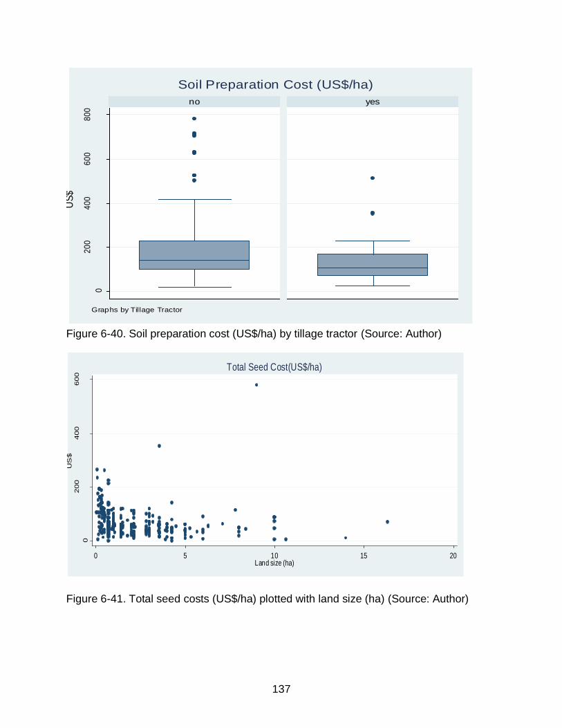
137
0
20
04
00
60
08
00
no yes
US
$
Graphs by Tillage Tractor
Soil Preparation Cost (US$/ha)
Figure 6-40. Soil preparation cost (US$/ha) by tillage tractor (Source: Author)
0
200
400
600
US
$
0 5 10 15 20Land size (ha)
Total Seed Cost(US$/ha)
Figure 6-41. Total seed costs (US$/ha) plotted with land size (ha) (Source: Author)

138
020
40
60
80
100
Sacks (
50 k
g)
less than 1ha 1-2.99ha 3-4.99ha equal or more than 5ha
Groups
Urea (50-kg sacks/ha)*Land Size Groups
Figure 6-42. Urea (50-kg sacks/ha) by land size groups (Source: Author)
10
15
20
25
30
35
Price (U
SD
$)
0 100 200 300 400Observations
Government Price of a Urea Sack(USD$) Market Price of a Urea Sack(USD$)
Other Price of a Urea Sack(USD$)
Urea Sack Prices (USD$)
Figure 6-43. Urea prices (US$/sack) of subsidized, real and black markets (Source: Author)

139
0
500
1,0
00
1,5
00
US
$/h
a
less than 1ha 1-2.99ha 3-4.99ha equal or more than 5ha
Groups
Total Cost Other Fertilizers/Foliars (USD$)*Land Size Groups
Figure 6-44. Total cost of other fertilizers (US$/ha) by land size groups (Source: Author)
0
200
400
600
800
US
$
less than 1ha 1-2.99ha 3-4.99ha equal or more than 5ha
Groups
Total Cost Herbicides/Pesticides(US$/ha)*Land Size Groups
Figure 6-45. Total cost of herbicides/pesticides (US$/ha) by land size groups (Source: Author)

140
0
100
200
300
400
US
$
0 5 10 15Number of HH Members
Total Cost Hired Labor(US$/ha)
Figure 6-46. Total cost of hired labor (Source: Author)
0
100
200
300
400
US
$
less than 1ha 1-2.99ha 3-4.99ha equal or more than 5ha
Groups
Total Cost Irrigation (US$/ha)*Land Size Groups
Figure 6-47. Total irrigation cost (US$/ha) by land size groups (Source: Author)

141
0
50
010
00
15
00
0
50
010
00
15
00
0 100 200 300 400 0 100 200 300 400
Less than 1 ha 1-2.99 ha
3-4.99 ha Equal/more than 5 ha
US
$
ObservationsGraphs by Land Size Groups
Total Harvest Cost (US$/ha)
Figure 6-48. Total harvest cost (US$) by land size groups (Source: Author)
050
100
150
200
kg
less than 1ha 1-2.99ha 3-4.99ha equal or more than 5ha
Groups
Rice Yield (kg/ha)*Land Size Groups
Figure 6-49. Rice yield (kg/ha) by land size groups (Source: Author)

142
0.5
10
.51
0 100 200 300 400 0 100 200 300 400
less than 1ha 1-2.99ha
3-4.99ha equal or more than 5ha%
ObservationsGraphs by Land Size
Rice Sacks for Sale
Figure 6-50. Rice sack sold (%) by land size groups (Source: Author)
0
50
00
10
00
0
0
50
00
10
00
0
0 100 200 300 400 0 100 200 300 400
Less than 1 ha 1-2.99 ha
3-4.99 ha Equal/more than 5 ha
US
$
ObservationsGraphs by Land Size Groups
Total Income (US$/ha)
Figure 6-51. Total income (US$/ha) by land size groups (Source: Author)

143
52.99%
47.01%
no yes
Credit Solicitation
Figure 6-52. Credit Solicitation (Source: Author)
Figure 6-53. Credit providers (Source: Author)

144
0
2,0
00
4,0
00
6,0
00
8,0
00
10
,000
US
$
less than 1ha 1-2.99ha 3-4.99ha equal or more than 5ha
Groups
Credit (US$)*Land Size Groups
Figure 6-54. Credit (US$) by land size groups (Source: Author)
Figure 6-55. Uses of the credit (Source: Author)

145
95.32%
4.675%
no yes
Rice Insurance
Figure 6-56. Rice insurance (Source: Author)
Figure 6-57. Main occupation (Source: Author)

146
Table 6-4. Time availability (hrs/day)
Variable Obs Mean Std. Err. Min Max
On-farm 385 6.05 2.45 0.50 18.00
Off-farm 385 1.75 3.12 0.00 14.00
Education 385 1.99 3.05 0.00 14.00
Source: Author
60%
40%
no yes
Non-work Income
Figure 6-58. Non-work income (Source: Author)

147
30
40
50
60
70
US
$
0 100 200 300 400Observations
Human Development Bonus(US$)
Figure 6-59. Human Development Bonus (US$) (Source: Author)

148
Table 6-5. Descriptive summary of dependent and independent variables
Variables Mean Std. Dev. Min Max
Intensity of Adoption (%) 49.70 40.69 0 100
Gender (1=male/0=female) 0.92 0.27 0 1
Age (years) 51.52 14.26 18 95
Education (years) 5.89 3.49 0 17
Agricultural education (1=yes/0= no) 0.2 0.4 0 1
Total operated land size (Ha) 2.01 2.18 0.04 16.33
Number of small kids in a household 1.3 1.39 0 8
Wealth index 0 1 -1.46 8.86
Flood or/and Drought affection (1=yes/0= no)
0.23 0.42 0 1
Time to get the main town (minutes) 23.5 15.34 1 120
Rented land (1=yes/0= no) 0.14 0.35 0 1
Past adoption (1=yes/0=no) 0.18 0.38 0 1
Subsidized Urea sacks (50 kg/ha) 3.19 4.97 0 42.25
Non-subsidized Urea sacks (50 kg/ha)
7.14 30.94 0 583.33
Labor cost (US$)/ha 188.06 43.73 0 395.77
Total other cost (US$/ha) 845.48 468.57 215.21 2674.33
Total yield (sacks 205 lb/ha) 63.37 21.51 14.08 200
Credit solicitation (1=yes/0= no) 0.47 0.5 0 1
Agricultural insurance (1=yes/0= no) 0.05 0.21 0 1
Risk aversion 2.8 0.52 1 3
UDP knowledge (1=yes/0= no) 0.09 0.29 0 1
Total on-farm hours/Ha 8.15 11.69 0.36 100
Total off-farm hours 1.75 3.12 0 14
Total education hours 1.99 3.05 0 14
Non-worked income (1=yes/0= no) 0.4 0.49 0 1
# of people of a religious group 4.81 43.63 0 650
# of people of a family group 2.11 4.29 0 65
# of people of an agricultural group/other group
106.08 296.84 0 3000
Source: Author

149
Table 6-6. Tobit model estimation of Intensity of Adoption
Regressors Observed Coef.
Boostrap Std. Err.
Z-value Marginal Effects
Gender (1=male/0=female) -1.08 14.88 -0.07 -0.28
Age (years) -0.14 0.30 -0.46 -0.04
Education (years) -0.51 1.17 -0.43 -0.13
Agricultural education (1=yes/0= no) -1.78 8.50 -0.21 -0.46
Total operated land size (Ha) -6.77* 1.48 -4.58 -1.74
Wealth index 3.77 8.06 0.47 0.97
Number of small kids in a household -5.05** 2.39 -2.11 -1.30 Flood or/and Drought affection (1=yes/0= no) -3.42 3.25 -1.05 -0.88
Time to get the main town (minutes) -0.71* 0.19 -3.69 -0.18
Rented land (1=yes/0= no) 19.72** 7.99 2.47 5.02
Past adoption (1=yes/0=no) -1.24 8.80 -0.14 -0.32
Subsidized Urea sacks (50 kg/ha) -1.43** 0.59 -2.43 -0.37
Non-subsidized Urea sacks (50 Kg/ha) 0.13 0.36 0.37 0.03
Labor cost (US$)/ha 0.04 0.08 0.51 0.01
Total other cost (US$/ha) 0.01 0.01 1.12 0.003
Total yield (sacks 205 lb/ha) -0.09 0.17 -0.52 -0.02
Credit solicitation (1=yes/0= no) 11.86** 5.89 2.01 3.05
Agricultural insurance (1=yes/0= no) 33.55*** 18.18 1.85 8.37
Risk aversion 10.85*** 5.60 1.94 2.79
UDP knowledge (1=yes/0= no) 20.35*** 12.12 1.68 5.17
Total on-farm hours/Ha 0.89*** 0.48 1.86 0.23
Total off-farm hours 1.56 0.98 1.58 0.40
Total education hours 1.38 1.00 1.37 0.35
Non-worked income (1=yes/0= no) 7.87 6.79 1.16 2.02
# of people of a religious group 0.001 0.77 0.00 0.0003
# of people of a family group 1.77*** 0.97 1.83 0.46 # of people of an agricultural group/other group -0.0032 0.01 -0.23 -0.001
Constant 40.70 32.16 1.27 -
Variance of the error term 53.47 2.75
Log likelihood -1397.80
Akaike's Information Criterion 7.41
Pseudo R2 0.035
Obs. Summary:
19 left-censored observations at SIA<=0
235 uncensored observations
131 right-censored observations at SIA>=100
Significant at *1%, **5% and ***10%. (Source: Author)

150
Table 6-7. Collinearity evaluation of the independent variables
VIF Tolerance R-Squared
Gender (1=male/0=female) 1.04 0.92 0.08
Age (years) 1.17 0.73 0.27
Education (years) 1.17 0.73 0.27
Agricultural education (1=yes/0= no) 1.04 0.92 0.08
Total rented/owned operated land size (Ha) 1.19 0.71 0.29
Number of small kids in a household 1.09 0.84 0.16
Wealth index 1.08 0.85 0.15
Flood or/and Drought affection (1=yes/0= no) 1.11 0.82 0.18
Time to get the main town (minutes ) 1.03 0.95 0.05
Rented land (1=yes/0= no) 1.04 0.92 0.08
Past adoption (1=yes/0=no) 1.08 0.85 0.15
Subsidized Urea sacks (50 kg/ha) 1.13 0.79 0.21
Non-subsidized Urea sacks (50 kg/ha) 1.09 0.84 0.16
Labor cost (US$)/ha 1.09 0.84 0.16
Total other cost (US$/ha) 1.20 0.69 0.31
Total yield (sacks 205 lb/ha) 1.14 0.77 0.23
Credit solicitation (1=yes/0= no) 1.12 0.80 0.20
Agricultural insurance (1=yes/0= no) 1.07 0.87 0.13
Risk aversion 1.02 0.96 0.04
UDP knowledge (1=yes/0= no) 1.08 0.86 0.14
Total on-farm hours/Ha 1.33 0.56 0.44
Total off-farm hours 1.06 0.88 0.12
Total education hours 1.07 0.87 0.13
Non-worked income (1=yes/0= no) 1.07 0.87 0.13
# of people of a religious group 1.05 0.91 0.09
# of people of a family group 1.01 0.97 0.03
# of people of an agricultural group/other group 1.13 0.78 0.22
Source: Author

151
-120
-80
-40
0
40
80
50 100 150 200 250 300 350
Intensity of Adoption Residuals
Figure 6-60. Intensity of Adoption Residuals (Source: Author)
0
10
20
30
40
50
-3 -2 -1 0 1 2
Series: Standardized Residuals
Sample 1 385
Observations 385
Mean -0.188757
Median -0.360610
Maximum 2.141331
Minimum -3.357998
Std. Dev. 1.037147
Skewness 0.044227
Kurtosis 2.043861
Jarque-Bera 14.79083
Probability 0.000614
Jarque-Bera Normality Test of Residuals
Figure 6-61. Jarque-Bera Normality test of Residuals (Source: Author)

152
CHAPTER 7 CONCLUSION REMARKS AND POLICY IMPLICATIONS
An ex-ante analysis was carried out to ascertain which factors may affect the
adoption process of Urea Deep Placement in the Ecuadorian Coast. This study only
takes into consideration small rice farmers in Daule and Santa Lucia cantons. The use
of primary data, which were collected through a survey instrument, made possible the
development of the descriptive and econometric analyses. Such analyses allow
responding the research question of this thesis. Consequently, I could obtain
interesting findings that are summarized in this section. Such findings would let to better
comprehend the decision making of rice farmers (and perhaps, farmers in general) on
the adoption of new technologies. Moreover, I provide recommendations for a suitable
introduction of UDP.
As a relevant observation, I noted that farmers were principally males (92.2%), but
behind these males there are wives also contributing with the rice activities directly or
indirectly. Some wives have the responsibility to purchase inputs, interacting with input
dealers and learning about rice business; a participation more intellectual than physical
on rice production.
I observed that few farmers mentioned to have adopted an
innovation/technology/technique, 18%. Additionally, only a 20% of the sample farmers
declared to have received agricultural instruction. This result would imply that farmers
need to be updated about new knowledge and new improved technology present in
agriculture currently. A further research is suggested on technology adoption and
agricultural education over time.

153
In spite of the fact that the smallest farmers obtained a better yield (kg/ha), their
production costs were the highest. Some of these farmers presented a negative net
income. There is a need of innovations that make rice business more profitable. For
instance, UDP would let these farmers not just increase their yield (income increase per
se) but also reduce their cost through Urea saving and weeding cost reduction; when
the labor requirement is supplied by family labor (remaining time not used by these
farmers). Also, UDP requires more labor that may augment costs. But, the labor
required might be satisfied by family labor, especially in small farm, without incurring in
any cost (Thomas P. Thompson and Joaquin Sanabria 2009). However, the opportunity
cost of working in rice production must be analyzed. As seen before, some households
are using considerable amount of hours on off-farm activities; being this cost high if
there exits more profitable jobs. Since farmers in these two rice producing zones have
rice production as main activity (there are not many jobs being offered in these zones
and Guayaquil city is the best place with more profitable alternatives but it is far away
from farmers’ household), one may think of a low opportunity cost and farmers would
dedicate the required hours for UDP production if adoption occurs. Thus, economy of
scale is produced by UDP having a better yield but reducing mean cost of rice
production as there are urea saving and weeding cost reduction.
Moreover, land size is significantly and negatively associated with Intensity of
Adoption. This effect was expected because UDP becomes more labor intensive as rice
cropland size increases. Moreover, UDP adopters were mainly small farmers in
Bangladesh. In Ecuador, 80% of the farmers are considered as small (less than 20 ha).
Therefore, the main adopters’ target would be those small farmers.

154
Another substantial variable was number of children in the household. This factor
was found inversely related to IA. As farmers have to take care of their small kids, they
would be constrained to dedicate time to experiment new technologies.
Also, while a farmer is closer to the market, he would be more willing to give more
land for UDP production. The two main constraints for market access were bad
conditions of the roads and lack of transportation. Construction of paved roads and
transportation service would not just work for UDP and other technology adoption but
also for the ease of rice trade, in general.
Being a land renter would apparently affect IA positively. These farmers are willing
to rent or possibly buy land to implement UDP as this technology produces benefits
such as urea saving and income increase, making rice business more attractive. Thus,
a land market is important to integrate more people to UDP production. In fact, with the
new land law being discussed at this moment, new rice farmers may be interest in
starting their rice production with this technology.
Additionally, the effects of three different markets of Urea fertilizer were able to be
differentiated: a subsidized market, a real market and a black market. In the end, only
the total number of subsidized Urea sacks had a significant and negative impact on IA. I
conclude that the effects of the subsidy and the black may be being reflected in this
variable. UDP might be perceived as a threat for those benefiting from the subsidy
(including those Urea resellers) because Urea saving with UDP may make government
reconsider about the subsidy. Hence, subsidies may be an important restraint for UDP
or other innovation adoption. However, the introduction of these types of technologies

155
that make farmers more competitive, requiring less help from government, are required
to reduce this fiscal pressure.
It seems that farmers have no problem with credit access; those who applied for
credit received the loan. These credits were important for rice production because this
money was spent on inputs mainly. On the other hand, special credit providers were the
“Chulqueros”, Rice Mill and friends; playing a relevant role in the development of rice
business (an important research to be developed is the impact of the aforementioned
credit sources on technology adoption). According to Tobit model, credit participation
determines IA positively; cash availability lets farmers try new techniques in their
production system. Thus, a credit market, with accessible agricultural credits, is strongly
recommended for the UDP adoption in rice production; the availability of these types of
credits could also work for adoption of other innovations related to the efficient uses of
rice production inputs as credits were used for inputs acquisition mainly.
Insurances were also significant and positive influence in the determination of
UDP adoption; being protected from natural disasters makes a farmer willing to try new
ideas as agricultural resources are ensured. As said before, Ecuador does not have a
developed insurance market because of different reasons. For instance, in agriculture
everyone is exposed to many natural disasters every year such as flood and drought;
this makes agricultural insurance market too risky and companies decide not to
participate in it. It is very important the current participation of the Ecuadorian
government in this market subsidizing such agricultural insurances. However, it seems
that there still a need of a development of an insurance market (e.g. only 18 farmers
mentioned to be a crop-insurance holder in this study). With a better accessibility to

156
these insurances and with an insurance culture, adoption of UDP and other improved
technology can take place in the Ecuadorian agriculture.
Moreover, the risk aversion measurement (the higher the value, the riskier) was
directly and significantly related to the IA. One can think of these risky farmers as
entrepreneurs. They are more willing to adopt new ideas, of course, with the availability
of resources such as money. Again, the importance of accessible credit market is
relevant for those more enthusiastic for adoption of UDP or any agricultural technique.
In estimating household time availability, I could note that those working on-farm
and off-farm dedicated almost the same hours to both activities, on average. I think of
two possible scenarios: 1) off-farm work would mean extra income that would be taking
as an extra capital for family rice production; or 2) other alternatives could be more
profitable than rice production and household time is being allocated to them over time;
this might mean a threat for rice production in the future. In the Tobit model, on-farm
hours are positively significant in explaining the Intensity of Adoption; those with more
hours spent on on-farm activities are more willing to give hectares for UDP production.
Farmers were also told that UDP is labor intensive and for that reason those spending
few hours on rice production hesitate to provide land for UDP production. Thus,
improved technologies are needed to make rice production more profitable. UDP is an
incentive that could maintain these people working in agriculture given the rice income
improvement and cost reduction.
Also, the majority of farmers belong to a formally built agricultural organization.
However, in asking famers for groups that may influence on their rice production
decisions, they named neighbors/friends, input suppliers and family as the most

157
influential. Additionally, with a simple methodology proposed by Bandiera and Rasul
(2002), social network effect may be caught without falling in the endogeneity problem
in the econometric model. Social network has a positive impact on IA which means that
a farmer would be more willing/reluctant to adopt UDP if there are potential/non-
potential adopters in his social network. In the end, the purpose was to identify the most
important social channels of these rice farmers. Working on the establishment of these
agricultural groups would be very decisive for the UDP adoption as these channels can
be used to spread UDP knowledge across all villages.
Despite the fact that the extension work carried out in Ecuador to diffuse UDP, the
promotion of this innovation is still needed: a 9.36% (36) of farmers knew about this new
fertilization method. Briquetting machine must be reproduced in order for farmers to
have access to briquettes and try this technology. Given the budget constraint, only one
briquetting machine was imported to experiment with UDP, obtaining very promising
results in term of yield and Urea saving. However, in the descriptive analysis of the
Double-bounded Questions, one could observe a surprising number of the studied
farmers willing to buy Urea briquette at a price higher than the normal Urea sack’s,
93.25% when introducing economic benefits/cost (WTP) and adding environmental
impacts (EWTP). Moreover, they showed their willingness to adopt UDP when they
adduced to give, on average, 49.70% of their land to produce with this technology. This
willingness could have been even greater if the diffusion of UDP would have continued.
In the Tobit estimation, having knowledge about UDP makes a farmer more interesting
in dedicating hectares for UDP production. Consequently, investments are needed to
start out this market. I encourage public and private investors to take part of this project

158
that have shown benefits for both firms and government (see International Fertilizer
Development Center 2008). Finally, one point that must be highlighted is the possible
lack of interest in environmental benefits of this technology. Education about
environment benefits must be considered in order to make farmers more aware of this
relevant resource (e.g. Daule River is a source of water for agricultural production and
for family consumption).
Considering the most significant variables, the potential adopter is defined as a
farmer having few hectares and small kids, being close to the market, renting land,
buying few subsidized Urea sacks, participating in the credit and insurance market,
taking risks, having UDP knowledge, spending most of his time on on-farm activities
and keeping potential UDP adopters in his social network.
There are two investigations that should be taken into consideration for UDP
development: 1) elaboration of a device to facilitate the Urea briquette placement (N. K.
Savant et al. 1991) and; 2) examination of UDP impact on the environment (reduction of
“N” going into the atmosphere and aquatic resources).
To sum up, important factors were identified, which would be determining adoption
of UDP, but also of any agricultural innovation in general. For instance, important
constrains for UDP adoptions would be a lack of credit and insurance markets. Hence,
information was provided to investors and policymakers of potential demanders of a
market with economic and social benefits. Finally, this thesis is a contribution to the
Ecuadorian agricultural technology adoption literature.

159
APPENDIX QUESTIONNAIRE (SPANISH VERSION)
Preguntas de Filtro
¿Usted maneja un cultivo de arroz? ____Si ____No(Pase a Sección 7: Salud, hoja 6)
¿Qué clase de manejo usted ha llevado en su cultivo de arroz?
____Arroz al trasplante ____Arroz Al voleo ____Otro: ¿Cuál?_________
¿Usted toma las decisiones sobre su cultivo de arroz?
____ Si ____No (siga a otra casa)
SECCIÓN 1: DIFUSIÓN DE LA APLICACIÓN PROFUNDA DE BRIQUETAS DE UREA
1. ¿Usted ha escuchado, visto o utilizado la Aplicación Profunda de Briquetas de Urea (las bolitas de Urea que se enterraban en el suelo)?
___Si ___No(pase sección 2: Redes sociales )
2. ¿De qué forma conoció la Aplicación Profunda de Briquetas de Urea (las bolitas de Urea
que se enterraban en el suelo)? (Ponga sí o no, o escoja el número de acuerdo a las claves)
3. ¿De qué forma por primera vez conoció personalmente los resultados de la Aplicación
Profunda de Briquetas de Urea (las bolitas de Urea que se enterraban en el suelo)?(Marque X o escoja el número de acuerdo a la clave4)
No he observado
Experimento en mi finca
Experimento en finca ajena
Observo a (clave4)
Otras (escriba cuales)
NOTA: SI OBSERVO (CLAVE4) A OTRA PERSONA LOS RESULTADOS DEL APBU, CONTESTE PREGUNTA 4. EN OTRO CASO PASE A LA PREGUNTA 5.

160
4. ¿Cuál es el nombre del dueño y la distancia aproximada desde su finca hasta la finca en donde usted observó los resultados de la Aplicación Profunda de Briquetas de Urea (las bolitas de Urea que se enterraban en el suelo)? (Distancia en tiempo que el encuestado le diga)
Unidad Cantidad Nombre
5. Si usted volvió a saber sobre la Aplicación Profunda de Briquetas de Urea (las bolitas de Urea que se
enterraban en el suelo), ¿hace cuánto tiempo y como volvió a saber? (Poner cero en cantidad si no supo nunca más y pasar a la pregunta 6 o 7)
6. NOTA: CONTESTE ESTA PREGUNTA SI EL ENCUESTADO EXPERIMENTO CON LAS BRIQUETAS
DE UREA EN LA PREGUNTA 3 O 5. Por favor, díganos la información aproximada sobre la producción con la Aplicación de briquetas de Urea de la última vez que la utilizó (VER HOJA PRODUCCIÓN CON APBU O PÁGINA 2).
7. De lo que ha escuchado, observado o experimentado, ¿Qué conocimiento tiene sobre la Aplicación
Profunda de Briquetas de Urea(las bolitas de Urea que se enterraban en el suelo)? (marque con una X el casillero correspondiente)
Poco Regular Bastante
¿Hace cuánto? ¿Cómo supo de nuevo sobre la Aplicación Profunda de briquetas de Urea (las bolitas de Urea que se enterraban en el suelo)?
Unidad Cantidad Reuniones en Asociaciones
Experimento en finca propia
Experimento en finca ajena
Conversando u Observando a (clave4)
Por esta encuesta
Otros (escriba cuales)

161
SECCIÓN 2: REDES SOCIALES
8. Indique todos los Grupo u Organización que usted u otro miembro de su hogar pertenece.
Miembro de su hogar
(Jefe del hogar,
esposa, hijo, etc.)
Tipo de Organización
/ Grupo (clave5)
Nombre del Grupo u
Organización
Número de personas dentro de su Grupo u Organización
Cuántas de estas
personas son
familiares
Participa en su grupo
voluntariamente (si/no)
Frecuencia de participación
Señale como es su participación en cada organización
Sem
anal
Mensual
Anual
No participa
Algo Activo
Muy Activo
Líder
SOLO SI HA USADO LA APLICACIÓN PROFUNDA DE BRIQUETAS DE UREAS: PRODUCCIÓN CON APBU
6. BASADA EN LA ÚLTIMA PRODUCCIÓN DE ARROZ CON LAS BRIQUETAS DE UREA (LA BOLITAS DE UREA QUE SE ENTERRABAN EN EL SUELO)
Ciclo Corto Producción de Arroz
Cultiv
o Rubros Unidad Cantidad
Valor Unitario
Observaciones
Arroz
Gastos en Semilla
$
Nombre de la semilla:
Tipo: R _ V_ H _
Gastos en Fertilizantes
¿Qué Cantidad de Urea usó y a quien se la compró?
Gobierno: ……... $
Casas Comerciales……... $
Otros:………. $ Quien:
¿Qué cantidad de NPK (Completo) usó? $
¿Qué cantidad de DAP (el de la pata, inicio) usó? $
Gastos en Foliares (escriba el costo total de todo el ciclo del cultivo de arroz) $

162
Gastos en Herbicidas/Malezas (escriba el costo total de todo el ciclo del cultivo de arroz) $
Gastos en Insecticida /Bichos y otros /líquidos (escriba el costo total de todo el ciclo del cultivo de arroz)
Gastos en pago a
Jornales
¿Qué cantidad de jornales/personas uso para el Trasplante? $
¿Qué cantidad de jornales/personas uso para Aplicaciones de Productos? $
¿Qué cantidad de jornales/personas uso para cosechar? $
Costos relacionados a Cosecha y Pilado: Cosechadora, transporte, cargada, sacos y pilada (escriba el costo total en el cultivo de arroz) $
Arroz Cosecha
En el último cultivo, ¿Qué cantidad cosechó?
En el último cultivo, ¿Qué cantidad dejó para consumo propio?
¿Qué cantidad y a qué precio vendió en Sacas (arroz en cascara)?
$
¿Qué cantidad y a qué precio vendió en Arroz Pilado?
$
De esta cosecha ¿Qué cantidad de dinero destinó para ahorro (escribe solo la cantidad de dinero ) $
a) ¿Cuánta área utilizó para producir con las briquetas de Urea? _________Cuadras
____________Tareas
C) Si alquilo las tierras, ¿cuánto pago en total? $_________
b) De esta área ¿Cuánto alquilo? (PONGA CERO SI NO ALQUILO Y PASE A LA
PREGUNTA 9) ______Cuadra _______Tareas
9. Por favor, conteste el siguiente conjunto de preguntas. (Para el encuestador: mencionar los grupos al encuestado en cada pregunta)
Grupos Preguntas
Vecinos Miembros de Asociación/Gru
po
Amigos no incluidos en
las anteriores categorías
Familiares
Dirigentes,
Presidentes o
líderes
Trabajadores de
extensión
Comerciante
Otros (detalle
nombre y que es para el
encuestado)
¿De quién aprendió el uso de fertilizantes? (puede escoger más de una opción)
¿Con qué frecuencia y con qué grupo usted habla sobre técnicas agrícolas? (Clave7)
Si tiene un problema ¿a quién pediría

163
un consejo o ayuda?
Elija los 3 grupos que influye más en sus decisiones sobre el manejo de su cultivo de arroz. (Siendo 1 el más importante y 3 el menos importante)
¿Cuál es el nombre de la persona a la que gente le pide consejos sobre el manejo de cultivos? (Anote en el nombre incluso cuando el encuestado mismo sea esa persona y cualquier otra identificación que sea posible encontrarlo) Nombre: _____________________ ¿Qué es para usted?:_______________ ¿A cuántos minutos de distancia esta la casa de esta persona?:_____________________
10. Indique con cuántos hombres y mujeres aproximadamente usted
conversa sobre técnicas agrícolas y a que grupo pertenecen. (escriba el número de personas en todos los grupos que diga el encuestado)
Grupo Religioso
Familiares Asociación/otro grupo/vecinos/amigos
Hombres
Mujeres
11. En general, ¿Cómo usted considera la comunicación entre los agricultores de su sector? Marque con una X
Baja Regular Indiferente Buena Muy Buena

164
SECCIÓN 3: ANTERIORES ADOPCIONES DE TÉCNICAS AGRÍCOLAS, PERCEPCIONES Y DISPONIBILIDAD A PAGAR
12. ¿Usted ha usado nuevas técnicas agrícolas en sus cultivos?
___Si ___No (pase 14) ____ No recuerdo(pase 14)
13. Si usted ha usado nuevas técnicas agrícolas en sus cultivos, ¿Cuáles fueron, hace cuánto tiempo las usó y cómo calificaría sus experiencias con los mismas?
¿Cuáles
fueron los
Cambios?
(Clave 6)
¿Hace cuánto
tiempo?
¿Cómo calificaría sus
experiencias con esas formas de
producir?
Unidad Cantidad Pésima Me dio
Igual
Buena
14. Por favor, responda si esta desacuerdo, indiferente o acuerdo sobre las siguientes oraciones (Marque con X)
Desacuerdo Indiferente Acuerdo
a) Usted comparte cualquier conocimiento agrícola con los agricultores de su sector.
b) TODOS los agricultores de su sector comparten experiencias del manejo de cultivos.
c) Usted utilizaría un nuevo método de aplicar la Urea en su cultivo de arroz, aunque otros no hayan usado este método.

165
15. Considerando los beneficios y costos de las Briquetas de Urea: Version 1:
a. ¿Estaría usted dispuesto a pagar por cada quintal de briquetas de Urea UN DÓLAR DE MÁS de lo que usted paga por la Urea normalmente?
Si (siga b)
b. Ya que está dispuesto a pagar un dólar, ¿Estaría usted dispuesto a pagar por cada quintal de briquetas de Urea UN DÓLAR y CINCUENTA CENTAVOS DE MÁS de lo que usted paga por la Urea normalmente?
Sí No
d. Sin importar las respuestas anteriores, En Su Mente ¿Cuánto usted estaría dispuesto a pagar por cada quintal de briquetas de Urea adicionalmente a lo que usted paga por la Urea normalmente?
$______
No (siga c)
c. Ya que no está dispuesto a pagar un dólar, ¿Estaría usted dispuesto a pagar por cada quintal de briquetas de Urea CINCUENTA CENTAVOS DE MÁS de lo que usted paga por la Urea normalmente?
Sí No
NOTA: PARA EL ENCUESTADOR: Debe de leerle este texto al encuestado antes se preguntarle la Pregunta 15: Explicación de la Aplicación Profunda de Briquetas de Urea y de sus Beneficios y Costos. La Aplicación Profunda de Briquetas de Urea (APBU) es una tecnología que convierte la Urea normal en briquetas (o pequeñas bolas de Urea) mediante una máquina llamada Briquetadora. Estas briquetas, que pesan alrededor de 2.7 a 4 gramos, son enterradas manualmente en medio de cuatro plantas en el suelo fangoso por debajo de la lámina de agua, después del trasplante y se lo hace por una sola vez en el ciclo de cultivo. Mediante las briquetas de Urea se puede evitar alrededor del 50% de la pérdida de la Urea por evaporación y escorrentías. De esta forma, las plantas podrán captar más el Nitrógeno contenido en la Urea. Los beneficios y costos de la Aplicación de las briquetas de Urea serían: Beneficios:
Con las briquetas de Urea se aplicaría de 4 a 4,5 quintales de Urea por hectáreas. Una reducción de Urea usada del 40%.
Incremento de la Producción de arroz del 25%, y por ende mayores ingresos.
Posible creación de pequeñas empresas encargadas de vender las briquetas de Urea y por ende generación de empleos.
Costos:
Se necesitaría dos jornales más por hectárea para aplicar la Urea.
Se debe tener comprados los 4 o 4,5 quintales de Urea para la aplicación entre los 15 a 20 días después del trasplante, ya que se fertiliza una solo vez durante todo el ciclo del cultivo. Po cual se debe hacer un solo gasto en todos los quintales de Urea al inicio

166
Version 2:
a. ¿Estaría usted dispuesto a pagar por cada quintal de briquetas de Urea TRES DÓLARES DE MÁS de lo que usted paga por la Urea normalmente?
Si (siga b)
b. Ya que está dispuesto a pagar tres dólares, ¿Estaría usted dispuesto a pagar por cada quintal de briquetas de Urea TRES DÓLARES Y CINCUENTA CENTAVOS DE MÁS de lo que usted paga por la Urea normalmente?
Sí No
d. Sin importar las respuestas anteriores, En Su Mente ¿Cuánto usted estaría dispuesto a pagar por cada quintal de briquetas de Urea adicionalmente a lo que usted paga por la Urea normalmente?
$______
No (siga c)
c. Ya que no está dispuesto a pagar tres dólares, ¿Estaría usted dispuesto a pagar por cada quintal de briquetas de Urea DOS DÓLARES Y CINCUENTA CENTAVOS DE MÁS de lo que usted paga por la Urea normalmente?
Sí No
Version 3:
a. ¿Estaría usted dispuesto a pagar por cada quintal de briquetas de Urea DOS DÓLARES DE MÁS de lo que usted paga por la Urea normalmente?
Si (siga b)
b. Ya que está dispuesto a pagar dos dólares, ¿Estaría usted dispuesto a pagar por cada quintal de briquetas de Urea DOS DÓLARES Y CINCUENTA CENTAVOS DE MÁS de lo que usted paga por la Urea normalmente?
Sí No
d. Sin importar las respuestas anteriores, En Su Mente ¿Cuánto usted estaría dispuesto a pagar por cada quintal de briquetas de Urea adicionalmente a lo que usted paga por la Urea normalmente?
$______
No
(siga c)
c. Ya que no está dispuesto a pagar dos dólares, ¿Estaría usted dispuesto a pagar por cada quintal de briquetas de Urea UN DÓLAR Y CINCUENTA CENTAVOS DE MÁS de lo que usted paga por la Urea normalmente?
Sí No

167
16. Considerando los beneficios y costos de las Briquetas de Urea, pero ahora considerando el beneficio ambiental:
Version 1: a. ¿Estaría usted dispuesto a pagar por cada quintal de briquetas de Urea UN DÓLAR DE MÁS de lo que usted paga por la Urea normalmente?
Si (siga b)
b. Ya que está dispuesto a pagar un dólar, ¿Estaría usted dispuesto a pagar por cada quintal de briquetas de Urea UN DÓLAR y CINCUENTA CENTAVOS DE MÁS de lo que usted paga por la Urea normalmente?
Sí No
d. Sin importar las respuestas anteriores, En Su Mente ¿Cuánto usted estaría dispuesto a pagar por cada quintal de briquetas de Urea adicionalmente a lo que usted paga por la Urea normalmente?
$______ No (siga c)
c. Ya que no está dispuesto a pagar un dólar, ¿Estaría usted dispuesto a pagar por cada quintal de briquetas de Urea CINCUENTA CENTAVOS DE MÁS de lo que usted paga por la Urea normalmente?
Sí No
NOTA: PARA EL ENCUESTADOR: Debe de leerle este texto al encuestado antes se preguntarle la Pregunta 16: Beneficios ambientales de la Aplicación Profunda de Briquetas de Urea. Sabiendo que los primeros beneficios y costos de las briquetas de Urea son: Beneficios: Reducción del uso de Urea en un 40%, Incremento de la producción de un 25% y una Posible generación de empleo. Costos: Aumento de los jornales utilizado y Compra al inicio de todos los quintales de Urea que van a ser aplicados. En cuanto al medio ambiente, cuando se utiliza la aplicación “Al voleo”, la cantidad de Urea que se puede estar perdiendo por escorrentías o por evaporación sería alrededor del 50%, lo cual afecta negativamente al medio ambiente. Mediante la aplicación con las briquetas de Urea se reduce la perdida de la Urea, consiguiendo los siguientes impactos ambientales:
• Se reduciría los gases, en este caso el Nitrógeno contenido en la Urea, que generan el Calentamiento global.
• Se reduciría el nitrógeno en los ríos, conservando el oxígeno en el agua y la vida acuática.
• Se evitarían enfermedades de las personas que beben aguas de los ríos, ya que se reduce el nitrógeno en esas aguas y el cual es malo para la salud cuando existe en grandes cantidades en el agua que es bebida.

168
Version 2:
Version 3:
a. ¿Estaría usted dispuesto a
pagar por cada quintal de
briquetas de Urea DOS
DÓLARES DE MÁS de lo
que usted paga por la Urea normalmente?
Si
(siga b)
b. Ya que está dispuesto a
pagar dos dólares, ¿Estaría
usted dispuesto a pagar por
cada quintal de briquetas de
Urea DOS DÓLARES Y CINCUENTA CENTAVOS
DE MÁS de lo que usted
paga por la Urea
normalmente?
Sí No
d. Sin importar las
respuestas anteriores,
En Su Mente ¿Cuánto
usted estará dispuesto a
pagar por cada quintal de briquetas de Urea
adicionalmente a lo
que usted paga por la
Urea normalmente?
$______ No
(siga c)
c. Ya que no está dispuesto a
pagar dos dólares, ¿Estaría
usted dispuesto a pagar por
cada quintal de briquetas de
Urea UN DÓLAR Y
CINCUENTA CENTAVOS
DE MÁS de lo que usted paga por la Urea
normalmente?
Sí No
17. NOTA: SE RESPONDE ESTA PREGUNTA SI ES QUE HUBO UNA DISPONIBILIDAD A PAGAR POR LAS BRIQUETAS DE UREA EN LAS PREGUNTAS 15 0 16. Dado que usted está dispuesto a pagar por las briquetas de Urea. ¿En cuántas cuadras-tareas usted estaría dispuesto a utilizar la Aplicación Profunda de Briquetas de Urea? ______Cuadra(s) ________ Tarea(s)
a. ¿Estaría usted dispuesto a pagar por cada quintal de briquetas de Urea TRES DÓLARES DE MÁS de lo que usted paga por la Urea normalmente?
Si (siga b)
b. Ya que está dispuesto a pagar tres dólares, ¿Estaría usted dispuesto a pagar por cada quintal de briquetas de Urea TRES DÓLARES Y CINCUENTAS CENTAVOS DE MÁS de lo que usted paga por la Urea normalmente?
Sí No
d. Sin importar las respuestas anteriores, En Su Mente ¿Cuánto usted estaría dispuesto a pagar por cada quintal de briquetas de Urea adicionalmente a lo que usted paga por la Urea normalmente?
$______
No (siga c)
c. Ya que no está dispuesto a pagar tres dólares, ¿Estaría usted dispuesto a pagar por cada quintal de briquetas de Urea DOS DÓLARES Y CINCUENTAS CENTAVOS DE MÁS de lo que usted paga por la Urea normalmente?
Sí No

169
SECCIÓN 4: SISTEMA DE PRODUCCIÓN
17. BASADA EN LA ÚLTIMA PRODUCCIÓN DE ARROZ, INDIQUE LOS COSTOS E INGRESOS QUE TUVO
a) ¿Cómo lleva su cultivo? Piscina______ Poza__________
Ciclo Corto Producción de Arroz
Cultivo Rubros Unidad Cantidad Valor
Unitario Observaciones
Arroz
Gasto en alquiler de cada unidad de terreno (Para el encuestador: el pago depende de la cantidad de tierra que se alquila para cultivar) $
Gasto en preparación de cada unidad de Terreno: arado y fangueado $
Gastos en Semilla
$
Nombre de la semilla:
Tipo: R _ V_ H _
Gastos en Fertilizantes
¿Qué Cantidad de Urea usó y a quien se la compró?
Gobierno: ……... $
Casas Comerciales……... $
Otros:………. $ Quien:
¿Qué cantidad de NPK (Completo) usó? $
¿Qué cantidad de DAP (el de la pata, inicio) usó? $
Gastos en Foliares (escriba el costo total de todo el ciclo del cultivo de arroz) $
Gastos en Herbicidas/Malezas (escriba el costo total de todo el ciclo del cultivo de arroz) $
Gastos en Insecticida /Bichos y otros /líquidos (escriba el costo total de todo el ciclo del cultivo de arroz)
Gastos en pago a Jornales
¿Qué cantidad de jornales/personas uso para el Trasplante? $
¿Qué cantidad de jornales/personas uso para Aplicaciones de Productos? $
¿Qué cantidad de jornales/personas uso para cosechar? $
Gastos en acceso al agua de riego
Paga a Junta de Riego_____ (cada cuanto tiempo y cuánto paga)
$
Paga por Riego por bomba_____ (gasto por cada galón de diesel para la bomba o pago con sacas de arroz)
$
Costos relacionados a Cosecha y Pilado: Cosechadora, transporte, $

170
cargada, sacos y pilada (escriba el costo total en el cultivo de arroz)
Arroz Cosecha
En el último cultivo, ¿Qué cantidad cosechó?
En el último cultivo, ¿Qué cantidad dejó para consumo propio?
¿Qué cantidad y a qué precio vendió en Sacas (arroz en cascara)?
$
¿Qué cantidad y a qué precio vendió en Arroz Pilado?
$
De esta cosecha ¿Qué cantidad de dinero destinó para ahorro (escribe solo la cantidad de dinero ) $
18. LLENE LA TABLA SI ES QUE TIENE OTROS CULTIVOS (PONGA EL NOMBRE DEL CULTIVO A LA IZQUIERDA) DE CICLO CORTO O CULTIVOS DE CICLO PERMANENTE
CICLO CORTO
Cultivo Rubros Unidad Cantidad Valor
Unitario Observaciones
De ciclo corto:
______
___
Costo Total Estimado (escriba el costo total solo) $
COSECHA
¿Qué cantidad cosechó? Área: ………
¿Qué cantidad dejó para consumo propio?
¿Qué cantidad vendió y a qué precio? $
De esta cosecha ¿Qué cantidad de dinero destinó para ahorro (escribe solo la cantidad de dinero ) $
CICLO PERMANENTE
De ciclo perman
ente: __________
Costo Total Estimado (escriba el costo total solo) $
COSECHA
¿Qué cantidad cosechó? Área: ………
¿Qué cantidad dejó para consumo propio?
¿Qué cantidad vendió y a qué precio? $
De esta cosecha ¿Qué cantidad de dinero destinó para ahorro (escribe solo la cantidad de dinero ) $
De ciclo perman
ente:
__________
Costo Total Estimado (escriba el costo total solo) $
COSECHA
¿Qué cantidad cosechó? Área: ………
¿Qué cantidad dejó para consumo propio?
¿Qué cantidad vendió y a qué precio? $
De esta cosecha ¿Qué cantidad de dinero destinó para ahorro (escribe solo la cantidad de dinero ) $
¿Cuánta área dedico a este cultivo? _____ cuadras _______tareas
¿Cuántos ciclos de cultivos de arroz usted tiene al año? __________ciclo(s)

171
19. Cuánto tiempo usualmente se demora en vender su producción de: Verano Invierno
Arroz Unidad: Cantidad:
Unidad: Cantidad:
Otro cultivo ¿Cuál?: Unidad: Cantidad:
Unidad: Cantidad:
20. ¿A cuántas piladoras usualmente usted puede ir a vender su producción de arroz? (si no va a las piladoras poner 0 y pasar 22)
_________piladora(s) _________piladora(s)
21. (No conteste si no va a vender su arroz a las piladoras). En las piladoras que usualmente usted vende su producción de arroz, díganos un número aproximado de cuanto otros productores de arroz venden su producción en esa misma piladora
________ productor(es) ________
productor(es)

172
SECCIÓN 5: MOVIMIENTOS DE DINERO
22. En el último año, ¿Usted pedio un préstamo? ____Si ____No(pase a 28A) 25. ¿En que gastó el préstamo
que hizo de mayor monto? Elija los 3 gastos más importantes, siendo 1 el más importante y 3 menos importante. Gastos (mencione los gastos al encuestado) ….Gastos en insumos o semillas, ….Gastos por Comprar o alquilar maquinaria, equipos, ….Gastos en repuestos para equipos vehículos, ….Gastos en arreglo de la casa, ….Gastos en pago de deudas, ….Gastos en familia: Salud, Educación, .... Gastos en entretenimiento, viajes, .... Otros gastos: ¿Cuáles?__________
26A. ¿Usted vendió su arroz a algún prestamista? … Si ….No(Pase 27) 26B. ¿El precio que vendió al prestamista fue precio al del mercado? … Si ….No 26C. ¿Cuál fue el precio y como lo vendió su arroz? Precio: $……. ¿Cómo? Por: ..... Saca …. Quintal
22A ¿A quién ha acudido? (marque con una X y puede elegir más de una opción)
22B Si le aprobaron el crédito, díganos un aproximado del monto que le prestaron y quien se lo presto. (Marque con una X en el casillero si no le aprobaron el préstamo)
Bancos Cooperativas Cajas de ahorro Banco Comunal Fundaciones Chulquero Piladoras Familiar o amigo Almacenes Otro: __________
No me aprobaron el préstamo (pase a 23) $______Bancos $______Cooperativas $______Cajas de ahorro $______Banco Comunal $______Fundaciones $______Chulquero $______Piladoras $______Familiar o amigo $______Almacenes $______Otro:___________
27. En el siguiente ciclo va a intentar pedir un préstamo a la misma persona/institución:
Si …. No ….
23. En caso de NO haberse concretado el préstamo, ¿Cuáles fueron los motivos? (Conteste y luego continúe desde la 27) ___Motivos del prestamista ____Motivos relacionados a usted ____Otros: ¿cuáles?_________
28A. ¿Usted tiene seguro agrícola? Si…. No….(pase 29) 28B. ¿Para qué cultivo? C1: Arroz…. C2:Mango… C3:Maíz… C4:Otro…… 28C. ¿Cuánto paga por cultivo? C1:……. Dólares, C2:……. Dólares, C3:…….Dólares; C4:…….Dólares 28D. ¿Cada qué tiempo? C1: Anual…, Trimestral…, Mensual…, Semestral…; C2: Anual…, Trimestral…, Mensual..., Semestral…; C3: Anual…., Trimestral…., Mensual…., Semestral….;C4:Anual…., Trimestral…., Mensual…., Semestral…. 28E. ¿Tiene algún seguro subsidiado por el gobierno? Si … No …; ¿Para qué cultivo? (escriba C1, C2, etc, según el cultivo): ……………..
24A. ¿Cuál fue el plazo de pago para el préstamo que hizo de mayor monto?(Marque con X, puede escoger solo 1 opción)
__Pagos diarios __ Pagos semanales __ Pagos quincenales __ Pagos mensuales __ Pagos trimestrales __Otros: ¿Cuáles?____________
24B. De acuerdo al plazo de pago, ¿Cuánto usted pago por este préstamo?
Pago:$___________
Nota: Si logro algún préstamo, conteste desde la 24 en adelante.

173
SECCIÓN 6: MERCADO LABORAL
29. TRABAJO ( Nota: Las siguientes preguntas están basadas en un día normal de trabajo (número de horas))
Integrante
Padre
¿Cuál es la principal fuente de ingreso? (Puede trabajar en agricultura o en otra cosa)
Agricultura ___ ; No agrícola __ No ingresos __
¿Cuántas horas usted trabaja en actividades agrícolas? hora(s)
¿Cuántas horas usted trabaja en actividades NO AGRÍCOLAS? ( Si contesta esta pregunta, ver a qué actividad se dedica en pregunta 33)
hora(s)
¿Cuántas horas le ocupa los estudios? hora(s)
¿Cuántas horas le ocupa en las actividades de casa?
Madre
¿Cuál es la principal fuente de ingreso?(Puede trabajar en agricultura o en otra cosa)
Agricultura ___ ; No agrícola __ No ingresos __
¿Cuántas horas su pareja trabaja en actividades agrícolas?
¿Cuántas horas su pareja trabaja en actividades NO AGRÍCOLAS? ( Si contesta esta pregunta, ver a qué actividad se dedica en pregunta 33)
¿Cuántas horas su pareja le ocupa los estudios?
¿Cuántas horas su pareja le ocupa en las actividades de casa?
Hijo
¿Cuál es la principal fuente de ingreso?(Puede trabajar en agricultura o en otra cosa)
Agricultura ___ ; No agrícola __ No ingresos __
¿Cuántas horas su hijo(a) trabaja en actividades agrícolas?
¿Cuántas horas usted trabaja en actividades NO AGRÍCOLAS? ( Si contesta esta pregunta, ver a qué actividad se dedica en pregunta 33)
¿Cuántas horas le ocupa los estudios?
¿Cuántas horas le ocupa en las actividades de casa?
30. ¿Cuántas personas en su hogar trabajan en la agricultura, incluyendo a usted?
__________persona(s)
31. ¿Cuántas personas en tu hogar trabajan en actividades NO AGRICOLAS, incluyen a usted?
__________persona(s)
32. ¿Cuántas personas en su hogar estudian, incluyendo a usted? __________persona(s)

174
34. EN EL ÚLTIMO AÑO, indique si recibió algún tipo de dinero que no es resultado del trabajo como por ejemplo de:
Monto en $ Frecuencia en la recibió este dinero Del dinero que recibió, ¿cuánto ahorró?
Familiares en otras partes del país Unidad: Cantidad:
Familiares en el extranjero Unidad: Cantidad:
Bono solidario Unidad: Cantidad:
Arriendos Unidad: Cantidad:
Ganancias financieras Unidad: Cantidad:
Donaciones Unidad: Cantidad:
Otros: _______________ Unidad: Cantidad:
33. ¿Trabaja Usted o alguien más de su familia en alguna otra actividad además de la agrícola que les de dinero? ___ Si(llene tabla de abajo) ___No(pase 34)
Nota: Responda las siguientes preguntas de acuerdo a las actividades que usted trabajó en el último año.
Preguntas Actividades
¿Cuál fue su Ingreso Aproximado por esta actividad?
¿Cada cuánto tiempo recibía este ingreso? ¿De este
monto cuanto ahorró?
Pesca $ ____Diario ____Semanal ___Mensual $
Proyectos forestales $ ____Diario ____Semanal ___Mensual $
Crianza de animales $ ____Diario ____Semanal ___Mensual $
Apicultura (Abejas) $ ____Diario ____Semanal ___Mensual $
Algún proceso Agroindustrial
$ ____Diario ____Semanal ___Mensual $
Turismo $ ____Diario ____Semanal ___Mensual $
Artesanía $ ____Diario ____Semanal ___Mensual $
Algún tipo de Comercio
$ ____Diario ____Semanal ___Mensual $
Alquiler de equipos $ ____Diario ____Semanal ___Mensual $
Otras: __________________
$ ____Diario ____Semanal ___Mensual $

175
SECCIÓN 7: SALUD
35. Responda el siguiente conjunto de preguntas:
a) ¿De dónde obtiene el agua para el uso diario?
Pozo …. Rio …. Agua potable por tubería ….. Agua potable por tanquero …. Agua embotellada…… Otro …..
b) ¿Usted usa el agua del rio o pozo para beber y cocinar?
Si ….. No …..
c) ¿Qué métodos usa para purificar el agua?
Química ….. Físico…. Filtros ….. Otros ….. Ninguno (Pase a pregunta e) …..
d) ¿Cuánto gasta por purificar esa agua?
…… dólares
POR CADA …. litros …. canecas …. tanques
CADA …. Día ….. Semana …… Mes
e) ¿Se ha enfermado del estómago en el último año?
Si ….. No ….. (Si responde NO; Pasar a pregunta m)
f) ¿Usted cree que esa enfermedad estuvo relacionada al tipo de agua que bebe?
Si ….. No …..(Si responde NO; Pasar a pregunta m)
g) ¿Dónde se hizo ver? Subcentro de salud de la comunidad…….
El pueblo más cercano ..... Cuál …………..
Ciudad ……… ¿Cuál?...................
h) ¿Cuán lejos queda el dispensario médico desde su casa?
….. minutos de distancia
i) ¿Cuánto gastó por transportarse hasta ese lugar?
….. Dólares
j) ¿Cuánto gastó en la consulta? ….. Dólares
k) ¿Cuánto gastó en la medicina? .…. Dólares
l) En total, ¿Cuántas veces se enfermó del estómago este último año?
……. Veces
m) ¿Otras personas dentro de su hogar se han enfermado del estómago en el último año?
Si …. No ….(Si responde NO; Pasar a pregunta 36)
n) ¿Cuántos? …………persona(s)
o) ¿Usted cree que esas enfermedades estuvieron relacionadas al agua que ellos beben?
Si … No ….

176
SECCIÓN 8: CARACTERÍSTICAS DEL HOGAR
36. Indique cuales de los siguientes bienes posee y en cuanto usted cree que están.
Ítem Valor Ítem Valor
__Casa __ Cosechadora
__ Tractor u otros equipos mayores __ Fumigadora u otras equipos
__ Bodega __ Carro
__ Piscina o Reservorio __ Planta eléctrica
__ Bombas de riego __ Empacadora
37.Su casa es: __ Propia; __ Alquilada; __ Prestada; __ Compartida
38.Servicios que posee: __ Agua Potable; __ Luz; __ Alcantarillado;
__ Teléfono; __ Alumbrado Público; ____Internet
39. Su casa está hecha de : __ Madera; __ Caña; __ Cemento; __ Mixta
40. ¿Cuál es la distancia en tiempo del pueblo más cercano y cuánto gasta en ir y regresar de allá? Unidad: Cantidad: ____ dólares
41. ¿Cuántos trasbordos necesita hacer hasta llegar allá? __ 1; __ 2; __3; __4; __5
42. ¿Cuántas personas están viviendo en su hogar? _______ adulto(s) ______niño(s) ______joven(es)
43. Cuál fue el gasto que hizo la última vez en
Alimentos Ropa Útiles Escolares Arreglos en la casa Otros: ¿Cuáles?
$ $ $ $ $
44A. ¿Durante el último año, su finca ha sufrido INUNDACIONES? Si ….. No …. 44B. ¿Durante el último año, su finca ha sufrido SEQUIAS? Si…. No….
45. De la última vez que sufrió estas INUNDACIONES Y/O SEQUIAS, qué porcentaje de tierra perdió en donde tenía cultivos de:
Arroz Mango Maíz Otros: 1) 2) 3) 4)
…. %(Inundación) …. % (Sequia)
…. %(Inundación) …. % (Sequia)
…. %(Inundación) …. % (Sequia)
1) …. %(Inundación) …. % (Sequia)
2) …. %(Inundación) …. % (Sequia)
3) …. %(Inundación) …. % (Sequia)
4) …. %(Inundación) …. % (Sequia)
46. ¿De la última vez que sufrió estos INUNDACIONES Y/O SEQUIAS, ¿cuánto gastó para recuperar la normalidad en su actividad agropecuaria? ….. Dólares (Inundación) …..Dólares (Sequia)

177
IDENTIFICACIÓN DEL HOGAR
Canton:___________ Sector:___________ Recinto/Barrio:____________ Tel.: _______
A29.Otras Indicaciones exactas para llegar a la casa:
GPS Código:
47. Actualmente ¿Cuánta área en total usted tiene para cultivar?
……….….Cuadras ………... Tareas
48. Señale si alquila o da en alquiler esta área para cultivo(marque con una X):
____doy en alquiler (1) ____ alquilo(2) _____Ninguna de las anteriores
1: …….….Cuadras ………... Tareas
2: …….…..Cuadras ………... Tareas
49. Actualmente ¿Cuánta área es destinada al cultivo de Arroz?
….….Cuadras .……... Tareas
…….….Cuadras ………... Tareas
50. Actualmente ¿Cuánta área es destinada a otros cultivos?
…….….Cuadras ………... Tareas
……….….Cuadras ………... Tareas
51. ¿Cuánta área tiene sin usar? ……….….Cuadras …………... Tareas
SECCIÓN 9: CARACTERÍSTICAS DEL INDIVIDUO
52. Sexo M F 53. Edad_______ años 54. Cuántos años en total ha estudiado Usted: ____ años
55. Máximo nivel de educación terminado
Analfabeto Secundaria Otros:¿Cuáles?
Primaria Universitaria Ninguno
56A ¿Usted ha recibido estudios agrícolas?
Sí No(pase 57)
56B ¿Qué temas estudio en esos cursos? (Clave6)
56C ¿Mediante quién o como recibió esos estudios agrícola?
____Gobierno ____ Organización ____ Ferias Agropecuarias ____ Escuelas
____ Colegios ____Universidades ____ Otros(cuales): __________
57. Estado civil ____Soltera(o) ____Viuda(o) ____Casada(o) ____Unión Libre. ____Divorciada(o)

178
LIST OF REFERENCES
Anderson, Kym, Lee A. Jackson, and Chantal P. Nielsen. 2005. "Genetically Modified Rice Adoption: Implications for Welfare and Poverty Alleviation." Journal of Economic Integration, 20(4): 771-788.
Banco Central del Ecuador. 2011. Encuesta de Coyuntura Sector Agropecuario. http://www.bce.fin.ec/documentos/PublicacionesNotas/Catalogo/Encuestas/Coyuntura/Integradas/etc201004.pdf.
Banco Nacional de Fomento. 2012. Microcreditos. https://www.bnf.fin.ec/index.php?option=com_content&view=category&id=5&Itemid=4&lang=es (accessed June 18, 2012).
Bandiera, Oriana, and Imran Rasul. 2006. "Social Networks and Technology Adoption in Northern Mozambique." The Economic Journal, 116(514): 869–902.
Barnum, Howard N., and Lyn Squire. 1979. "An Econometric Application of the Theory of the Farm-Household." Journal of Development Economics, 6: 79-102.
Bennett, J. 1995. "Biotechnology and the Future of Rice Production." GeoJournal, 35(3): 333-335.
Besley, Timothy, and Anne Case. 1993. "Modeling Technology Adoption in Developing Countries." The American Economic Review, Papers and Proceedings of the Hundred and Fifth Annual Meeting of American Economic Association, 83(2): 396-402.
Breustedt, Gunnar, Jörg Müller-Scheeßel, and Uwe Latacz-Lohmann. 2008. "Forecasting the Adoption of GM Oilseed Rape: Evidence from a Discrete Choice Experiment in Germany." Journal of Agricultural Economics, 59(2): 237–256.
Buttel, Frederick H., Martin Kenney, and Jr. Jack Kloppenburg. 1985. "From Green Revolution to Biorevolution: Some Observations on the Changing Technological Bases of Economic Transformation in the Third World." Economic Development and Cultural Change, 34(1): 31-55.
Bwire, Joseph. 2008. "Factors Affecting Adoption of Improved Meat Goat (Boer) Production in Rangelands of Sembabule District." http://news.mak.ac.ug/documents/Makfiles/theses/Bwire_Joseph.pdf.
Cameron, A. C., and Pravin K. Trivedi. 2010. Microeconometrics Using Stata, Revised Ed. Texas: Stata Press.
Castillo, María J. 2011. "Seguro Agrícola en Ecuador: ¿Un Servicio a la Comunidad o un Negocio Rentable?" Paper presented at Coffe Break Opinion desde la Academia, Graduate School of Management ESPAE, Guayaquil, Ecuador.

179
Chiriboga, Manuel, and Brian Wallis. 2009. Diagnostico de la Pobreza Rural en Ecuador y Respuestas de Politica Publica. Quito: Centro Latinoamericano para el Desarrollo Rural.
Conley, Timothy G., and Christopher R. Udry. 2010. "Learning about a New Technology: Pineapple in Ghana." American Economic Review, 100(1): 35–69.
Contreras, Orlando D., and Marcelo Espinosa. 2010. "Diseño y Cálculo de una Máquina para Producir Briquetas de Urea.” http://www.dspace.espol.edu.ec/bitstream/123456789/8027/1/Dise%C3%B1o%20y%20C%C3%A1lculo%20%20de%20una%20m%C3%A1quina%20para%20producir%20Briquetas%20de%20Urea.pdf.
Dalrymple, Dana. 1986. Development and Spread of High-Yielding Rice Varieties in Developing Countries. Washington, D.C.: Agency for International Development.
Dekker, M. 2006. "Estimating Wealth Effects without Expenditure Data: Evidence from Rural Ethiopia." Ethiopian Journal of Economics, 15(1): 35-54.
Dobermann, Achim. 2012. "IRRI Agronomy Challenge: How Much Fertilizer." http://www.irri.org/index.php?option=com_k2&view=item&id=11712%3Airri-agronomy-challenge-how-much-fertilizer&lang=en.
Doss, Cheryl R. 2006. "Analyzing Technology Adoption Using Microstudies: Limitations, Challenges, and Opportunities for Improvement." Agricultural Economics, 34: 207–219.
Doss, Cheryl R., and Michael L. Morris. 2000. "How does Gender Affect the Adoption of Agricultural Innovations? The Case of Improved Maize Technology in Ghana." Agricultural Economics, 25(1): 27–39.
D'Souza, Gerard E., Douglas Cyphers, and Tim T. Phipps. 1993. "Factors Affecting the Adoption of Sustainable Agricultural Practices." Agricultural and Resource Economics Review, 22(2).
Ecuadorian Const. of 2008, art. CDI.
Escuela Superior Politecnica del Litoral, University of Florida, and USDA-PL-480. 2008. "Implementación de un Programa para Mejoramiento Del Ingreso de Pequeños Productores de Arroz en el Litoral Ecuatoriano: Aplicación Profunda de Briquetas de Urea y Microcrédito." Unpublished.
Evenson, R. E., and D. Gollin. 2003. "Assessing the Impact of the Green Revolution, 1960 to 2000." American Association for the Advancement of Science, 300(5620): 758-762.
Feder, Gershon, and Dina L. Umali. 1993. "The Adoption of Agricultural Innovations A Review." Technological Forecasting and Social Change, 43: 215-239.

180
Fernandez-Cornejo, Jorge, Chad Hendricks, and Ashok K. Mishra. 2005. "Technology Adoption and Off-Farm Household Income: The Case of Herbicide-Tolerant Soybeans." Journal of Agricultural and Applied Economics, 37(3): 549-563.
Food and Agriculture Organization of the United Nations. 2012. FAOSTAT http://faostat.fao.org/?lang=en. (accessed May 15, 2012).
Food and Agriculture Organization of the United Nations. 2011. "Rice Market Monitor." http://www.fao.org/docrep/013/am156e/am156e00.pdf.
Foster, A. D., and M. R. Rosenzweig. 1995. "Learning by Doing and Learning from Others: Human Capital and Technical Change in Agriculture." The Journal of Political Economics, 103(6): 1176-1209.
Gedikoglu, Haluk, and Laura M.J. McCann. 2007. "Impact of Off-Farm Income on Adoption of Conservation Practices." Paper presented at the Annual Meeting from American Agricultural Economics Association, Oregon, TN.
Gianessi, Leonard, Sujatha Sankula, and Nathan Reigner, ed. 2003. Plant Biotechnology: Potential Impact for Improving Pest Management in European Agriculture: A Summary of Nine Case Studies. Washington, D.C.: The National Center for Food and Agricultural Policy.
Greene, William H. 2012. Econometric Analysis, 7th Ed. Boston: Prentice Hall.
Gujarati, Damodar N., and Dawn C. Porter. 2009. Basic Econometrics, 5th Ed. New York: McGraw-Hill Irwin.
Hannan, Timothy H., and John M. McDowell. 1984. "The Determinants of Technology Adoption: The Case of the Banking Firm." The RAND Journal of Economics, 15(3): 328-335.
Heckathorn, Douglas D. 1997. "Respondent-Driven Sampling: A New Approach to the Study of Hidden Populations." Social Problems, 44(2): 174-199.
Herdt, R. W., and C. Capule. 1983. Adoption, Spread, and Production Impact of Modern Rice Varieties in Asia. Los Banos: International Rice Research Institute.
Herrera, Paúl, Katherine Jiménez, Graciela Prado, and Ramón Espinel. 2010. "Capital Social y Desarrollo Comunitario: El Caso de las Juntas de Usuarios del Sistema de Riego del Valle del Daule." In Tierra y Agua: Interrelaciones de un Acceso Inequitativo, ed. Edgar Isch, and Alex Zapatta, 111-130. Quito: Sistema de Investigación sobre la Problemática Agraria en el Ecuador.
Hildebrand, P. E., L. Andrade, W. Bowen, R. Espinel, P. Herrera, P. Jaramillo, I. Medina, S. Mora, A. Santos, C. Toledo, et al. 2008. "Condiciones Agro-Socio Económicas y Ecológicas de los Diversos Sistemas de Producción de Arroz de Pequeños Productores en Guayas y Los Ríos, Ecuador." Unpublished.

181
Hogset, Heidi. 2005. "Social Network and Technology Adoption." Paper presented at the American Agricultural Economics Association Annual Meeting, Providence, Rhode Island.
Hubbell, Bryan J., Michele C. Marra, and Gerald A. Carlson. 2000. "Estimating the Demand for a New Technology: Bt Cotton and Insecticide Policies." American Journal of Agricultural Economics, 82: 118–132.
Instituto Nacional de Estadística y Censos. 2011. "Sistema Agroalimentario del Ecuador." http://www.ecuadorencifras.com/sistagroalim/pdf/Arroz.pdf
Instituto Nacional de Estadística y Censos. 2012. Ecuador en Cifras. http://www.ecuadorencifras.com/cifras-inec/main.html (accessed June 10, 2012).
Instituto Nacional de Preinversion. 2011. "Enfoques De Preinversion." http://www.preinversion.gob.ec/pmo/enfoquespreinversion.pdf
International Fertilizer Development Center. 2008. "Expansion of Urea Deep Placement Technology in 80 Upazilas of Bangladesh during Boro 2008: An Assessment of Project Impact." Unpublished.
International Fertilizer Development Center. 2012. Fertilizer Deep Placement (FDP). http://www.ifdc.org/Expertise/Fertilizer/Fertilizer_Deep_Placement_(UDP). (accessed March 20, 2012)
International Food Policy Research Institute. 2002. "Green Revolution: Curse Or Blessing?” http://www.ifpri.org/sites/default/files/pubs/pubs/ib/ib11.pdf.
International Rice Research Institute. 2012. http://www.irri.org. (accessed June 6, 2012).
Jain, Rajni, Alka Arora, and S.S. Raju. 2009. "A Novel Adoption Index of Selected Agricultural Technologies: Linkages with Infrastructure and Productivity." Agricultural Economics Research Review, 22: 109-120.
Keelan, Conor, Fiona S. Thorne, Paul Flanagan, Carol Newman, and Ewen Mullins. 2009. "Predicted Willingness of Irish Farmers to Adopt GM Technology." The Journal of Biotechnology Management and Economics, 12(3&4): 394-403.
Kennedy, Peter. 2008. A Guide to Econometrics, 6th Ed. Malden: Wiley-Blackwell.
Khanna, Madhu. 2001. "Sequential Adoption of Site-Specific Technologies and its Implications for Nitrogen Productivity: A Double Selectivity Model." American Journal of Agricultural Economics, 83(1): 35-51.

182
Kristjanson, P., I. Okike, S. Tarawali, B. B. Singh, and V. M. Manyong. 2005. "Farmers' Perceptions of Benefits and Factors Affecting the Adoption of Improved Dual-Purpose Cowpea in the Dry Savannas of Nigeria." Agricultural Economics, 32: 195–210.
Kropiwnicka, Magdalena. 2005. "Biotechnology and Food Security in Developing Countries: The Case for Strengthening International Environmental Regimes." Journal on Science and World Affairs, 1(1): 45-60.
Loh, Lawrence, and N. Venkatraman. 1992. "Diffusion of Information Technology Outsourcing: Influence Sources and the Kodak Effect." Information Systems Research, 3(4): 334-358.
Lu, Bao-Rong, and Allison A. Snow. 2005. "Gene Flow from Genetically Modified Rice and its Environmental Consequences." BioScience, 55(8): 669-678.
Lupin, M. S., J. R. Lazo, N. D. Le, and A. F. Little. 1983. Alternative Process for Urea Supergranules. Muscle Shoals: International Fertilizer Development Center.
Ministerio de Agricultura, Ganaderia, Acuacultura and Pesca. 2011. El MAGAP, a través de la Unidad de Seguro Agrícola se reúne con Productores Arroceros del Cantón Daule. http://www.magap.gob.ec/mag01/index.php/prensa-boletinesprensa/1783-seguro-agricola-se-reune-con-productores-arroceros-del-canton-daule. (accessed March 12, 2012).
Ministerio de Agricultura, Ganaderia, Acuacultura and Pesca. 2012. Plan Tierras. http://www.magap.gob.ec/mag01/index.php/boletines-viceministerio-desarrollo-rural/122. (accessed June 1, 2012).
Ministerio de Inclusion Economica y Social 2012. Programa de Proteccion Social. http://www.pps.gob.ec/PPS/PPS/QuienesSomos.aspx. (accessed June 01, 2012)
Mora, Samuel, and Paul Herrera. 2010. "Comparación de dos Tecnologías de Aplicación de Nitrógeno (Urea) en Diferentes Niveles en el Cultivo de Arroz: Aplicación Profunda de Briquetas de Urea y la Aplicación Tradicional Alvoleo." http://www.dspace.espol.edu.ec/bitstream/123456789/11362/10/Resumen%20CICYT.pdf.
Ngoc Chi, Truong T. 2008. "Factors Affecting Technology Adoption among Rice Farmers in the Mekong Delta through the Lens of the Local Authorial Managers: An Analysis of Qualitative Data." Omonrice, 16: 107-112.
Nnadi, Fidelia N., and Chidi Nnadi. 2009. "Farmers’ Sustained Adoption Decision Behaviors of Maize/Cassava Intercrop Technology in Imo State: Lessons for Extension Policy Development." World Rural Observations, 1(2): 87-92.

183
Nyanga, Progress H., Fred H Johnsen, Jens B Aune, and Thomson H Kalinda. 2011. "Smallholder Farmers’ Perceptions of Climate Change and Conservation Agriculture: Evidence from Zambia." Journal of Sustainable Development, 4(4): 73-85
Organización de las Naciones Unidas para la Agricultura y la Alimentación, Fondo Internacional de Desarrollo Agrícola, and Programa Mundial de Alimentos. 2002. "La Reducción de La Pobreza y el Hambre: La Función Fundamental de la Financiación de la Alimentación, la Agricultura y el Desarrollo Rural." Paper presented at Conferencia Internacional sobre la Financiación para el Desarrollo, Monterrey, Mexico.
Pannell, David J. 2007. "Influences on Technology Adoption in Different Phases." http://www.pannelldiscussions.net/2007/06/.
Pingali, Prabhu, and Terri Raney. 2005. "From the Green Revolution to the Gene Revolution: How Will the Poor Fare?" Agricultural and Development Economics Division of Food and Agriculture Organization of the United Nations Working Paper 05-09.
Qaim, Matin. 2005. "Agricultural Biotechnology Adoption in Developing Countries." American Journal of Agricultural Economics, 87(5): 1317–1324.
Qualls, D. J., Kimberly L. Jensen, Christopher D. Clark, Burton C. English, James A. Larson, and Steven T. Yen. 2012. "Analysis of Factors Affecting Willingness to Produce Switchgrass in the Southeastern United States." Biomass & Bioenergy, 39: 159-167.
Rahman, Sanzidur. 2008. "Determinants of Crop Choices by Bangladeshi Farmers: A Bivariate Probit Analysis." Asian Journal of Agriculture and Development, 5(1): 29-42.
Raju, S. S., and Ramesh Chand. 2008. "Agricultural Insurance in India Problems and Prospects." National Centre for Agricultural Economics and Policy Research, 8: 1-80.
Savant, N. K., and P. J. Stangel. 1990. "Deep Placement of Urea Supergranules in Transplanted Rice: Principles and Practices." Fertilizer Research, 25: 1-83.
Savant, N. K., P.S. Ongkingco, I.V. Zarate, F.M. Torrizo, and P.J. Stangel. 1991. "Urea Briquette Applicator for Transplanted Rice." Fertilizer Research, 28: 323-331.
Simtowe, Franklin, and Manfred Zeller. 2007. "The Impact of Access to Credit on the Adoption of Hybrid Maize in Malawi: An Empirical Test of an Agricultural Household Model Under Credit Market Failure." Munich Personal RePEc Archive, 45: 1-28.

184
Singleton, Royce A., Jr., and Bruce C. Straits. 2010. Approaches to Social Research, 5th Ed. New York: Oxford University Press.
Sistema de Información Nacional de Agricultura, Ganadería, Acuacultura y Pesca. 2012. III Censo Nacional Agropecuario. 2012. http://www.magap.gob.ec/sinagap/index.php?option=com_wrapper&view=wrapper&Itemid=400 (accessed June 3, 2012).
Sistema de Información Nacional de Agricultura, Ganadería, Acuacultura y Pesca. 2012. Principales Productos de Importacion. http://www.magap.gob.ec/sinagap/index.php?option=com_wrapper&view=wrapper&Itemid=100 (accessed May 29, 2012).
Staal, S. J., I. Baltenweck, M.M. Waithaka, T. DeWolff, and L. Njoroge. 2002. "Location and Uptake: Integrated Household and GIS Analysis of Technology Adoption and Land use, with Application to Smallholder Dairy Farms in Kenya." Agricultural Economics, 27(3): 295–315.
Sunding, David, and David Zilberman. 2001. "Chapter 4 The Agricultural Innovation Process: Research and Technology Adoption in a Changing Agricultural Sector." In Handbook of Agricultural Economics, Vol. 1A, ed. Bruce L. Gardner, and Gordon C. Rausser, 207-261. North-Holland: Elsevier science.
Swinton, S. M., and J. Lowenberg-deboer. 2001. "Global Adoption of Precision Agriculture Technologies: Who, when and Why?" Paper presented at the Third European Conference on Precision Agriculture, Montpellier, France.
Thompson, Thomas P., and Joaquin Sanabria. 2009. The Division of Labor and Agricultural Innovation in Bangladesh: Dimensions of Gender. Muscle Shoals: International Center for Soil Fertility and Agricultural Development.
Wu, Haitao, Shijun Ding, Sushil Pandey, and Dayun Tao. 2010. "Assessing the Impact of Agricultural Technology Adoption on Farmers’ Well-being using Propensity-Score Matching Analysis in Rural China." Asian Economic Journal, 24(2): 141–160.

185
BIOGRAPHICAL SKETCH
Jorge Avila was born in the city of Guayaquil, Ecuador. He went to the university
Escuela Superior Politecnica del Litoral “ESPOL”. While specializing in Economic
Politics and Theory, he received fundamental classes such as Econometrics,
Microeconomics, Macroeconomics, Public Economics and Development and Economic
Welfare Theory. At 23 years old, he finished his bachelor’s studies and started his
professional life as a research assistant at Rural Research Center and Graduate School
of Management of ESPOL. He was engaged in works such as Social Corporate
Responsibility and Socioeconomic Analysis. With Dr. Espinel and Dr. Herrera, he
developed a research paper “Determinants of the Current Trends of Agricultural
Products Consumer and Markets” which was presented in the academic event held by
the Latin American Council of School Administration (CLADEA, in Spanish). Afterwards,
he was included in the Urea Deep Placement Project carried out by ESPOL and UF. His
function was to promote and understand rice farmers’ livelihood system and technology
adoption process for his coming master’s thesis. In 2010, he began his master’s
program which was funded by ESPOL, UF, PL-480 of USDA and the Secretaria
Nacional de Educacion Superior, Ciencias, Tecnologias e Innovacion “SENESCYT”.
While at UF, he complemented his economic studies with two practical and innovative
tools in agriculture: Geographic Information System “GIS” and Network Analysis.
Currently, his research interests are associated with agricultural technology adoption,
social networks functionality and biodiversity. Taking advantage from his econometric
and GIS knowledge, he expects to combine his research interests during his PhD
program which would begin in August of 2012.


![Threshold Responses of Macroinvertebrate Communities to ... · The Guayas River basin consists of two large tributaries: the Daule River and the Babahoyo River [14]. The two rivers](https://static.fdocuments.in/doc/165x107/5f96e32d0838c5545b4da96f/threshold-responses-of-macroinvertebrate-communities-to-the-guayas-river-basin.jpg)


